In February 2024, Vision Pro, Apple’s long-awaited extended reality (XR) headset, hit stores. It is Apple’s stab at the consumer XR market, but XR is not how Apple describes it. Instead, when it was announced last summer, Apple CEO Tim Cook said the headset marks the dawning of the era of spatial computing. “You’ve never seen anything like this before,” he added.
Greg Milner
That is not quite true.
The term spatial computing dates to the 1980s. Its modern definition entered the lexicon in 2003. Simon Greenwold, a graduate student in the Program in Media Arts and Sciences at the Massachusetts Institute of Technology (MIT), described spatial computing wherein a human interacts with a machine, and that machine retains and manipulates referents to objects and spaces in the real world.
But spatial computing extends back even further. It has been the cornerstone of geographic information system (GIS) technology since the software programs debuted in the late 1960s. Indeed, the theoretical foundation of GIS is that it is not only possible but inherently useful to retain and manipulate real objects within some form of virtual space.
In the first GIS programs, virtual space was synonymous with cartographic space. Spatial computing means using maps to organize large amounts of data in a visually intuitive manner.
The Roots of Spatial Computing
Early geospatial technology pioneers applied the concepts of such theorists as Ian McHarg, who described the world as a series of layers of information that exist and interact in the same physical spaces. If we analyze any spot on Earth, we encounter such informational layers as elevation, soil type, hydrology, biology and land use.
GIS brought this idea to life. The technology allows us to visualize and analyze layers of data on a map. In this way, GIS has become a key integrator of information about our world, from science to engineering to commercial operations.
Through innovation, GIS has grown beyond the bounds of mere 2D map layers to generate maps that are, in effect, 1:1-scale 3D models we call geospatial digital twins.
The major benefit of geospatial digital twins is the ability to provide maximum context. This is especially useful for smart planning of our urban environments. For example, architects can use a digital twin to test how their proposals will fare in such situations as flooding and extreme heat brought about by climate change. City planners can understand the effects of large-scale shifts in the urban environment with interventions focused on enhancing livability. The combination of visualization and hard data allows them to predict impacts and modify plans before making expensive changes to the physical world.
Spatial Computing and Digital Twins
Each advance in GIS technology has improved our ability to visualize, link and manipulate real objects and spaces in a digital realm.
GIS has evolved to offer truly immersive experiences. In particular, the combination of GIS and game engines such as Unreal and Unity has transformed the process of large-scale infrastructure projects.
In Brisbane, Australia, for example, a digital twin of the ongoing subway construction has been used to display progress. People can walk virtually through planned subway tunnels and stations. This contextual experience helps project leads show Brisbanites how the work is shaping up.
The experience also allows planners, architects, engineers and construction workers to make decisions with more information than could be provided by a paper map or even a traditional digital twin. They can stand on a platform and see how the design elements of a station will look to people moving through it.
Spatial Computing to Visualize What Could Be
Digital twins can be crystal balls. The virtual spaces can be reconfigured to model different versions of an environment. In practical terms, digital twins allow various stakeholders to have the same vision. This is especially useful in the age of climate change.
Planners and architects can test different versions of a project. If they are designing a subdivision in a coastal community, they can calculate the flooding and storm surge that will likely occur from storms of different magnitudes. Just as important, they can visualize this data, inhabit it, and study it with maximum context.
At root, what they are doing is investigating spatial relations against a realistic backdrop of the world. For the subdivision, these objects include homes, streets, streetlights, and parks, and what matters is their existence in relation to water under multiple scenarios. This is spatial computing: manipulating referents to real objects in a virtual world that, unlike the real one, can be changed at will.
Spatial Computing to Visualize Hidden Real Spaces
Immersive environments also offer the promise of displaying a world that is real and already exists yet remains largely invisible.
Public utilities and other companies involved with underground infrastructure have been some of the most enthusiastic adopters of digital twins because the experience can reveal critical connections buried beneath the earth — made visible without the need to dig.
In 2017, the Toms River Municipal Utilities Authority (TRMUA) in Toms River, New Jersey, began using mixed reality (MR) headsets to help crews find underground utility assets for electric, gas, water, telecommunications and sewer services.
GIS stores the location of these assets, and MR displays the underground infrastructure. Traditionally, utilities display this detail on a 2D map. What MR provides is maximum context. Workers in the field can visualize exactly what is under their feet—and see how it’s related spatially to what is all around them.
TRMUA credits MR with saving time and lowering the chances of breaking connections in the networks residents rely on for modern living — savings in the tens of thousands of dollars every day.
Many utilities have since followed TRMUA’s lead. MR setups serve multiple purposes, including training new employees and sharing information between teams in the field and staff in the office.
One utility industry publication recently noted that what these systems ultimately provide is the elimination of guesswork. The ability to know exactly where an asset is located — and to understand how changes will affect the area around it — leads to increased efficiency and customer satisfaction.
The World in Sharper Focus
Apple’s Vision Pro headset is not the only recent example of XR rebranded as spatial computing. Meta and Microsoft have also marketed their XR headsets — Quest 3 and Hololens, respectively — as spatial computers.
Spatial computing will continue its mainstreaming. Eventually, it will likely be the norm. As XR hardware increases in number and power, more organizations will look to unlock the value of all the spatial data recorded in GIS. Being able to experience data will add further value to the systems and workflows that create it.
GIS pioneers began exploring the outer limits of spatial computing a half-century ago. More recently they have realized its potential for smarter urban planning, climate risk mitigation, management of operations across industries and virtual exploration of real-world systems or scenarios via geospatial digital twins. Someday soon, those limits will be reachable by anyone.
As GIS users have learned through the decades, when we get a better sense of where we are in relation to things we care about, we can create the world we want to see.
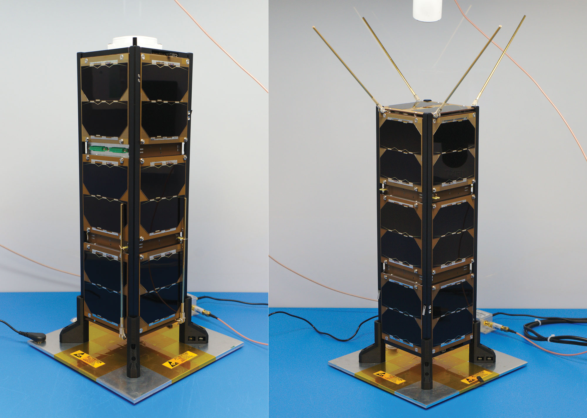
Figure 1: Bobcat-1, with communications antenna stowed (left) and deployed (right). Bobcat-1 measures approximately 10 x 10 x 30 centimeters. (All figures except FIGURE 3 provided by the authors)
Bobcat-1 was a three-unit CubeSat developed and built at Ohio University’s Avionics Engineering Center in Athens, Ohio, and was named after the university’s mascot. FIGURE 1 shows Bobcat-1 with and without its antenna deployed. The satellite was launched to the International Space Station in October 2020 (see FIGURE 2) and deployed into low-Earth orbit (LEO) the following month (see FIGURE 3). In April 2022, it deorbited and burned up in Earth’s atmosphere as planned, after a successful 17-month mission, lasting eight months longer than anticipated. The last signal decoded from Bobcat-1 was received only about 10 minutes before the satellite’s demise, from an altitude of about 109 kilometers, by an amateur radio operator (ZR6AIC) near Johannesburg, South Africa, associated with SatNOGS, a global network of amateur satellite-networked open ground stations.
The main mission of the Bobcat-1 CubeSat was to evaluate the feasibility of GNSS-to-GNSS time offset monitoring from LEO. One of the secondary mission objectives was GNSS spectrum monitoring.
In addition, Bobcat-1 also included a side-mission, hosting a software-defined GPS/Galileo receiver developed by the University of Padova and Qascom — an Italian engineering company providing security solutions in satellite navigation and space cybersecurity — to perform its in-space demonstration and testing. This receiver served as a prototype for the receiver soon to be launched on NASA’s Lunar GNSS Receiver Experiment (LuGRE) mission.
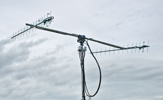
Communications and control of the satellite utilized the 70-centimeter amateur radio satellite band (435-438 MHz) at a typical data rate of 60 kilobits per second and were primarily conducted using a dedicated ground station on the roof of the engineering building at Ohio University (see FIGURE 4). In total, Bobcat-1 collected and downlinked more than 656 megabytes of data during its lifetime. Over the course of the mission, Bobcat-1’s firmware was updated in-orbit on six occasions, allowing for minor enhancements to the data collection system.
Figure 2: Bobcat-1 launches aboard the Cygnus NG-14 resupply mission to the International Space Station. (All figures except FIGURE 3 provided by the authors.)
BACKGROUNDS: GNSS-TO-GNSS TIME OFFSET
GNSS-to-GNSS time offsets — also referred to as GNSS inter-constellation time offsets, inter-system biases or XYTOs — are among the critical parameters for full GNSS interoperability. Users with poor GNSS visibility, such as high-altitude spacecraft, which operate above the GNSS constellations, often do not have enough satellites in view to enable an accurate solution and can experience high dilution of precision. These users could benefit from XYTO estimates provided externally, assuming their receiver-characteristic inter-system biases (ISBs) are calibrated.
To determine a user solution using measurements from a single GNSS constellation, one must solve for four unknown parameters: the user’s spatial coordinates and the receiver-to-system time offset. This means that a minimum of four satellites must be visible to solve for a user solution. If a user has sufficient visibility of satellites from different constellations, a multi-GNSS solution can be determined. However, when applying measurements from multiple constellations, an additional unknown is added for each constellation used. For example, for a user solution incorporating measurements from both GPS and Galileo, one needs to solve for five unknowns: the user’s spatial coordinates, the receiver-to-GPS time offset, and the receiver-to-Galileo time offset. Since each constellation’s time scale is independent of the others, the inter-system time offset between the time scales leads to a prominent bias in a multi-constellation solution. Inter-system time offsets between GPS, Galileo, GLONASS, and BeiDou are generally expected to range from 10 to 100 nanoseconds, resulting in 3 to 30 meters of possible positioning error.
System-to-system time offsets are currently estimated by extensive networks of ground stations, such as those used by the International GNSS Service Multi-GNSS Experiment (MGEX). In addition, GNSS service providers often broadcast XYTO estimates in their navigation messages.
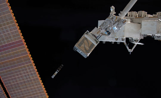
Figure 3: Bobcat-1 is deployed into low-Earth orbit by the Nanoracks CubeSat Deployer alongside SPOC, a CubeSat developed by the University of Georgia. (Photo: NASA)
So, why would estimating XYTOs from LEO be of interest?
Low-Earth orbit enables high GNSS visibility. The approximately 90-minute orbital period allows for observations from nearly all GNSS satellites multiple times per day. This enables high visibility of multiple satellites from each constellation, in turn enabling high observability of constellation parameters such as XYTOs, leveraging satellite-characteristics errors. In addition, tropospheric errors are absent and multipath is limited and can be bounded based on the CubeSat’s dimensions and geometry. Exploiting measurements from LEO could provide additional measurements and independent monitoring of the XYTO estimates provided by ground networks.
However, to estimate system-characteristic XYTOs, the receiver-characteristic biases need to be calibrated. The target is to reach accuracy of approximately 1 nanosecond or possibly lower. Therefore, the error sources need to be evaluated, mitigated, or bounded.
Figure 4: Bobcat-1’s dedicated ground station on the roof of Stocker Center in Athens, Ohio. (All figures except FIGURE 3 provided by the authors.)
Although the ionospheric effects are lower in LEO than on Earth, they cannot be neglected. Therefore, dual-frequency ionospheric delay estimates must be applied. To do so, the receiver’s inter-frequency biases (IFBs), which can introduce errors on the order of nanoseconds, need to be calibrated, as well as the satellite differential code biases (DCBs), orbit and clock errors and receiver antenna group delay. An additional challenge introduced by the LEO environment is the wide range of temperatures to which the receiver is subjected. Over a single orbit, the receiver’s temperature can vary from approximately 0 to 50 degrees Celsius. The effects of these temperature variations cause fluctuations in the receiver’s IFBs, which need to be evaluated and calibrated. Pre-launch measurements in a controlled environment using a climate chamber and two receivers of the same make and model were used for calibration. We have detailed those measurements elsewhere.
The multipath error can be bounded, as a first approximation, to 10 centimeters (or about 0.3 nanoseconds in equivalent signal delay) due to the dimensions of the CubeSat. However, given the mount of the antenna is on one of the CubeSat’s two 10 × 10 centimeter faces, that upper bound is in practice much smaller and the multipath error is mostly negligible.
Finally, the last remaining major error sources to be calibrated are the receiver ISBs. The main goal, to demonstrate the feasibility of LEO-CubeSat-based monitoring of GNSS XYTOs, requires showing the stability (or the repeatability) of the receiver biases in orbit.
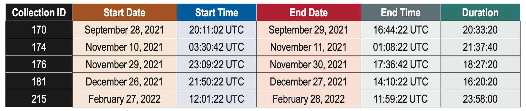
Table 1: Summary of data collections discussed in this article.
DATA COLLECTION
Bobcat-1’s primary payload was a NovAtel OEM719, a triple-frequency multi-GNSS receiver, enabling measurements on all frequencies from GPS, GLONASS, Galileo and BeiDou, as well as the regional navigation satellite systems (RNSSs) QZSS and NavIC. The measurements were collected and downloaded, for post-processing purposes.
Pseudorange and carrier-phase measurements, as well as carrier-to-noise-density ratio estimates, were collected, together with the receiver’s position and velocity estimates, and other parameters such as the temperature measured by the two sensors embedded in the receiver. In limited instances, power spectral density measurements and in-phase and quadrature (I/Q) component samples were collected to support the secondary mission, GNSS spectrum monitoring. The limited downlink capacity of the satellite constrained these measurements to short time intervals.
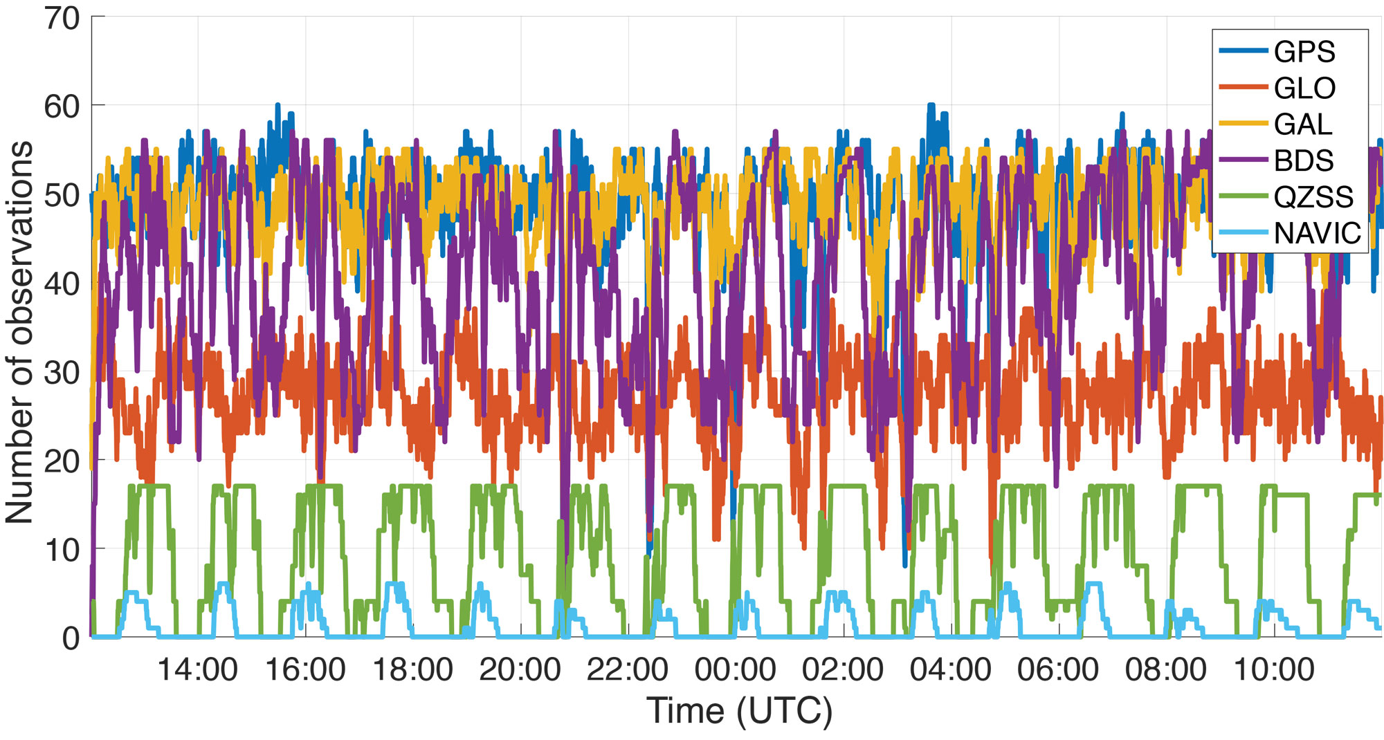
Figure 5: Number of observations recorded by Bobcat-1 from each GNSS constellation during a data collection started on February 27, 2022.
The goal of the mission is to estimate the XYTOs for all the GNSS constellations. However, in this article only the Galileo-to-GPS time offset (GGTO) is considered. The Galileo Performance Reports published by the European Union Agency for the Space Programme (EUSPA) provide information on the accuracy of the GGTO broadcast parameters, which are typically within approximately 3 nanoseconds of the true GGTO. Therefore, the broadcast GGTO provides a point of comparison and reference for Bobcat-1’s estimates.
A summary of the data collections considered in this work is provided in TABLE 1. These data collections are among the longest recorded by Bobcat-1. As an example, FIGURE 5 shows Bobcat-1’s data collection for February 27, 2022. It should be noticed that data collections were initiated from the control station at Ohio University when the CubeSat was in view, and each data collection would start only when the satellite’s battery voltage was above a defined threshold. The collection would stop safely if a minimum voltage threshold was reached. The data sets collected during the first months of the mission had durations limited to one to four hours, since the minimum battery voltage threshold was set conservatively. However, as the mission continued, data collections recorded in the last several months before deorbiting were configured with lower thresholds, enabling continuous data collections with durations of up to 24 hours. During the longer data collections, the sampling period was set to 20 seconds to reduce the total quantity of data stored and downlinked. The work described here focuses on a select few data collections that span a period of five months between September 28, 2021, and February 27, 2022.
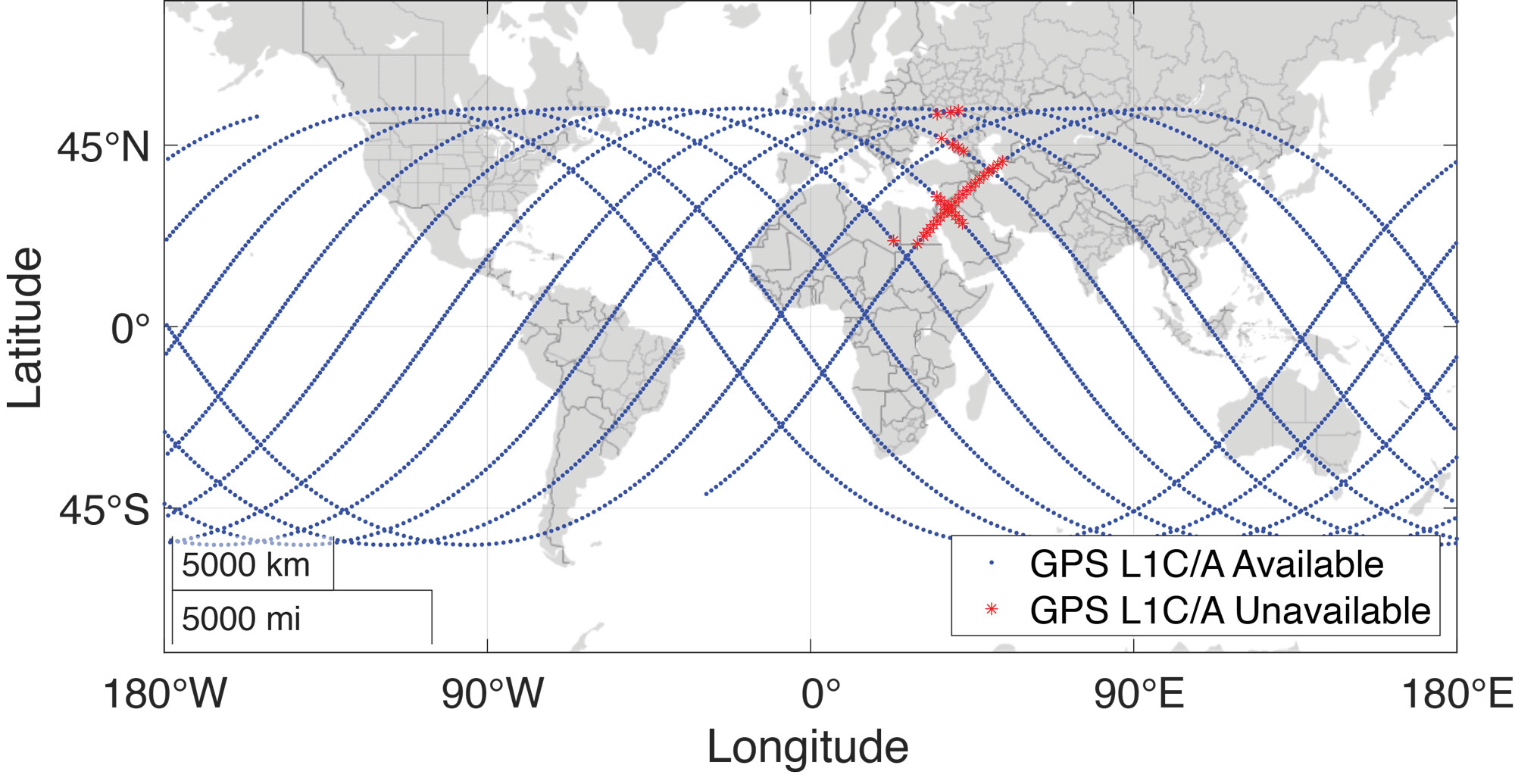
Figure 6: Bobcat-1’s ground track during a data collection for XYTOs estimation held in February 2022, approximately 24-hours long. Note that the blue dots correspond to the positions (latitude and longitude) of Bobcat-1. The red stars indicate that even if the position was calculated thanks to a multi-frequency and multi-GNSS solution, GPS L1 C/A measurements were not available. Analysis of the carrier-to-noise-density ratio measurements and comparison with the available spectrum measurements showed that in correspondence to those positions interference was present.
The data contain multi-frequency measurements from all systems, with an average of 180 observations made per sample. The maximum number of observations at once was 217. While multi-frequency measurements were collected from all constellations, this analysis only uses single-frequency measurements from two constellations: GPS L1 C/A and Galileo E1C.
RESULTS
There are two simple approaches to calculating inter-constellation time offsets: one involves computing multiple single-constellation user solutions, and the other involves a single multi-constellation user solution. Each approach has slightly different effects in terms of error propagation. In the first approach, the XYTOs can be calculated by taking the difference of the independently calculated receiver-to-system time offsets. This method requires at least four satellites from each constellation to be visible. In the second approach, all the receiver-to-system time offsets for all constellations involved in the solution are solved simultaneously. This reduces the number of measurements required per-constellation, with the minimum number of measurements needed being equal to the number of unknown state variables.
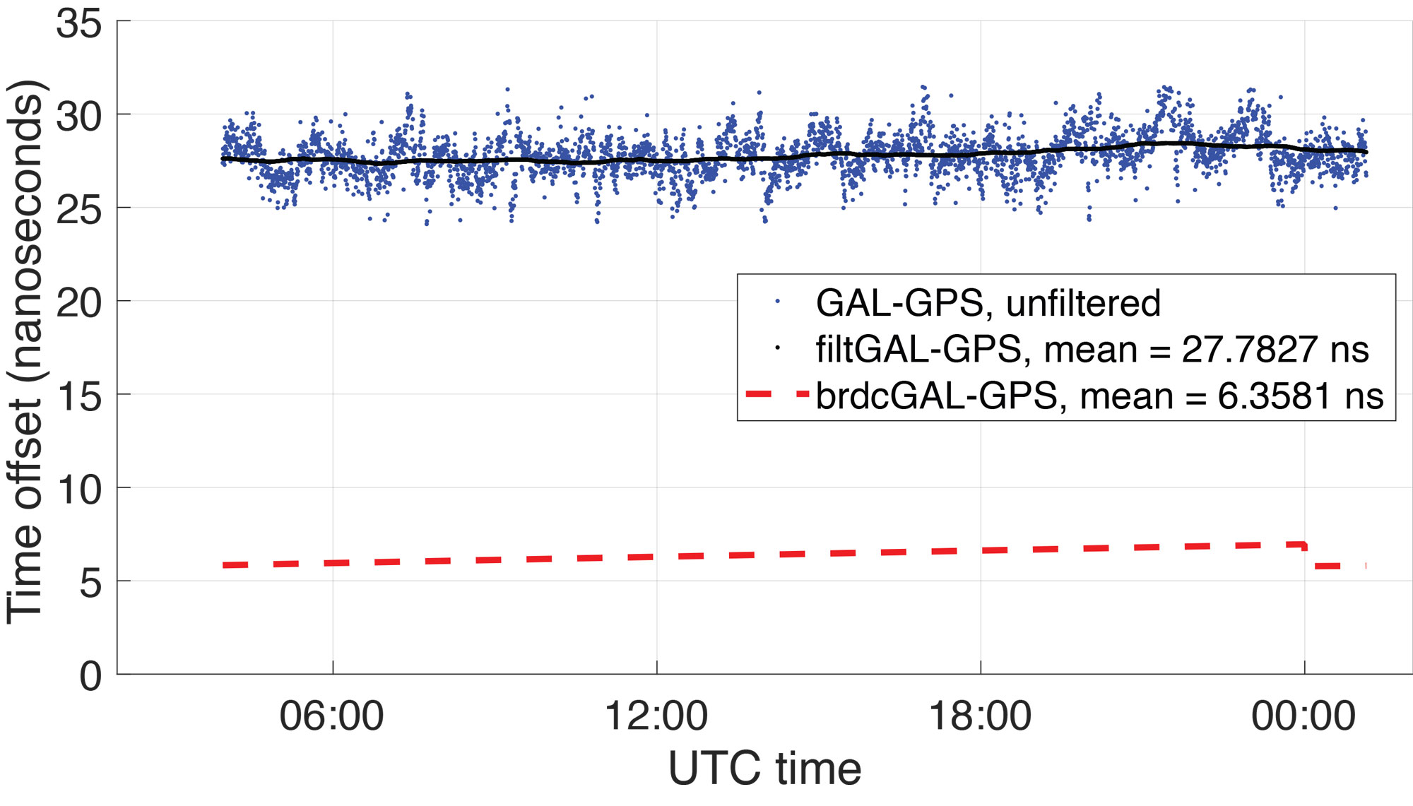
Figure 7: Broadcast GGTO (red) compared to Bobcat-1 Galileo-GPS time offset estimate, before calibration (blue) and filtered estimate (black). The results are related to data collection 181, started on December 27, 2021, which lasted about 16 hours (more than 10 orbits). The estimates’ variations, on the order of ±5 nanoseconds, are mainly due to temperature effects during the orbit and here are simply represented with a moving average.
In general, the latter method improves the XYTOs’ solution availability since the receiver-to-system time offsets for each system can be calculated with even fewer than four measurements from each system. For each sample point, the user solution was determined using this method, and the GGTO estimate was calculated by taking the difference of the receiver-to-GPS time offset and the receiver-to-Galileo time offset. This method allows the XYTO to be estimated by the receiver even when visibility is degraded. For example, as shown in FIGURE 6, Bobcat-1’s data collections are affected by interference, mostly on GPS L1, in some regions. Points where interference was believed to be present are marked by red stars on Bobcat-1’s ground track shown in the figure, specifically denoting points where the number of tracked GPS L1 C/A signals drops below four. For each sample point, the user solution was determined using the method discussed above, and the GGTO estimate was calculated by taking the difference of the receiver-to-GPS time offset and the receiver-to-Galileo time offset.
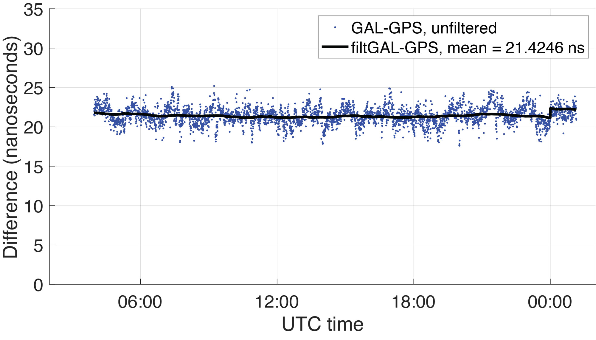
Figure 8: Difference between Bobcat-1 estimate and GGTO. The residual is mainly an estimate of the receiver inter-system bias that even pre-calibration shows to be stable in orbit as shown in Table 2.
FIGURE 7 shows (in blue) the GGTO estimate using Bobcat-1 measurements (data collection 181, started on December 27, 2021, and lasted about 10 orbits). The plotted values are the estimate of the system-to-system bias (GGTO) from which the receiver-specific ISB (Galileo-to-GPS) has not yet been removed. The oscillations visible in the unfiltered GGTO estimates are the result of temperature effects on the receiver. They can be mitigated by applying the calibrations made during pre-launch climate chamber testing, though for this analysis the estimates are simply filtered using a moving average (shown in black in the figure). Note that the abrupt change in the broadcast GGTO about 21 hours after the collection start corresponds to the start of a new day in UTC time, when a new estimate of the broadcast GGTO parameters was provided.
In FIGURE 8, the difference between the Bobcat-1 estimate of the GGTO and the broadcast GGTO is plotted (raw, in blue, and filtered with a moving average, in black). This is an estimate of the Bobcat-1 receiver’s Galileo-to-GPS ISB, which needs to be stable and repeatable in orbit, to enable accurate estimates of the true GGTO. As Figure 8 indicates, the receiver ISB shows stability even before calibration, showing periodical variations mainly due to temperature changes over the orbit.
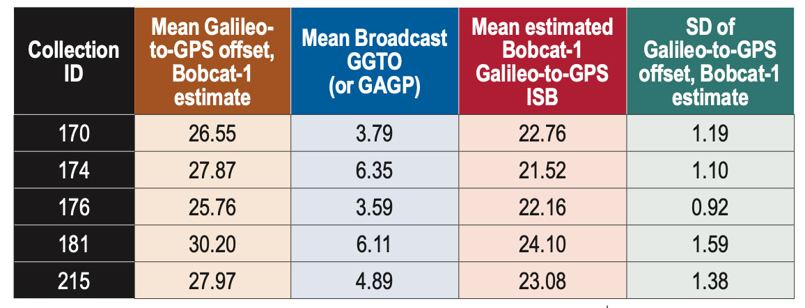
TABLE 2 summarizes some results over a five-month period. Only the longest data collections were considered, but the shorter ones are also under analysis to provide a longer and denser observation window. From the data in Table 2, the Bobcat-1 receiver’s mean Galileo-to-GPS ISB, estimated by comparison with the broadcast GGTO, shows a standard deviation, pre-calibration, of less than 1.5 nanoseconds over five months. Considering that the accuracy on the broadcast GGTO is expected to be ≤ 3 nanoseconds, this estimate of the receiver ISB shows that its stability over time may enable accurate XYTO monitoring from LEO.
Table 2: Bobcat-1 Galileo-to-GPS time offset vs broadcast GGTO, for different data collections over about five months. All figures in columns two through five are in nanoseconds.
The implementation of the receiver bias calibration, including the temperature effects, will refine this result. The final test will include assessing the performance of the calculated system XYTO, utilizing it in the solution of another receiver previously calibrated and at a known location.
CONCLUSIONS
Results of five 15+ hour data collections spanning a period of five months are compared. The difference between the broadcast GGTO and the GGTO estimate calculated using data from Bobcat-1 appears to be stable within 1.5 nanoseconds. Observing the in-orbit data and comparing it with the data collected previously in a controlled environment in the laboratory, a high correlation is observed between the bias change over time and the measured receiver temperature. The mitigation of this effect will enable stability of our receiver characteristic GGTO estimate to within 1 nanosecond. These experimental results suggest that a few multi-GNSS receivers in LEO could provide a method to monitor XYTOs in near real time, providing redundancy and diversity to the ground-network-based estimation system.
ACKNOWLEDGMENTS
The authors would like to acknowledge NASA’s Satellite Communication and Navigation Office (SCaN), NASA’s Glenn Research Center, NASA’s CubeSat Launch Initiative (CSLI), and Ohio University for funding the Bobcat-1 CubeSat mission. Additionally, we thank Kevin Croissant and Gregory Dahart, previous student members of the Bobcat-1 team, and Dr. Frank van Graas, Ohio University Professor Emeritus and former faculty member of the Bobcat-1 team.
This article is based on the paper “Receiver-specific GNSS Inter-system Bias in Low-Earth Orbit” presented at ION ITM 2023, the 2023 International Technical Meeting of the Institute of Navigation, Long Beach, California, January 23-26, 2023.