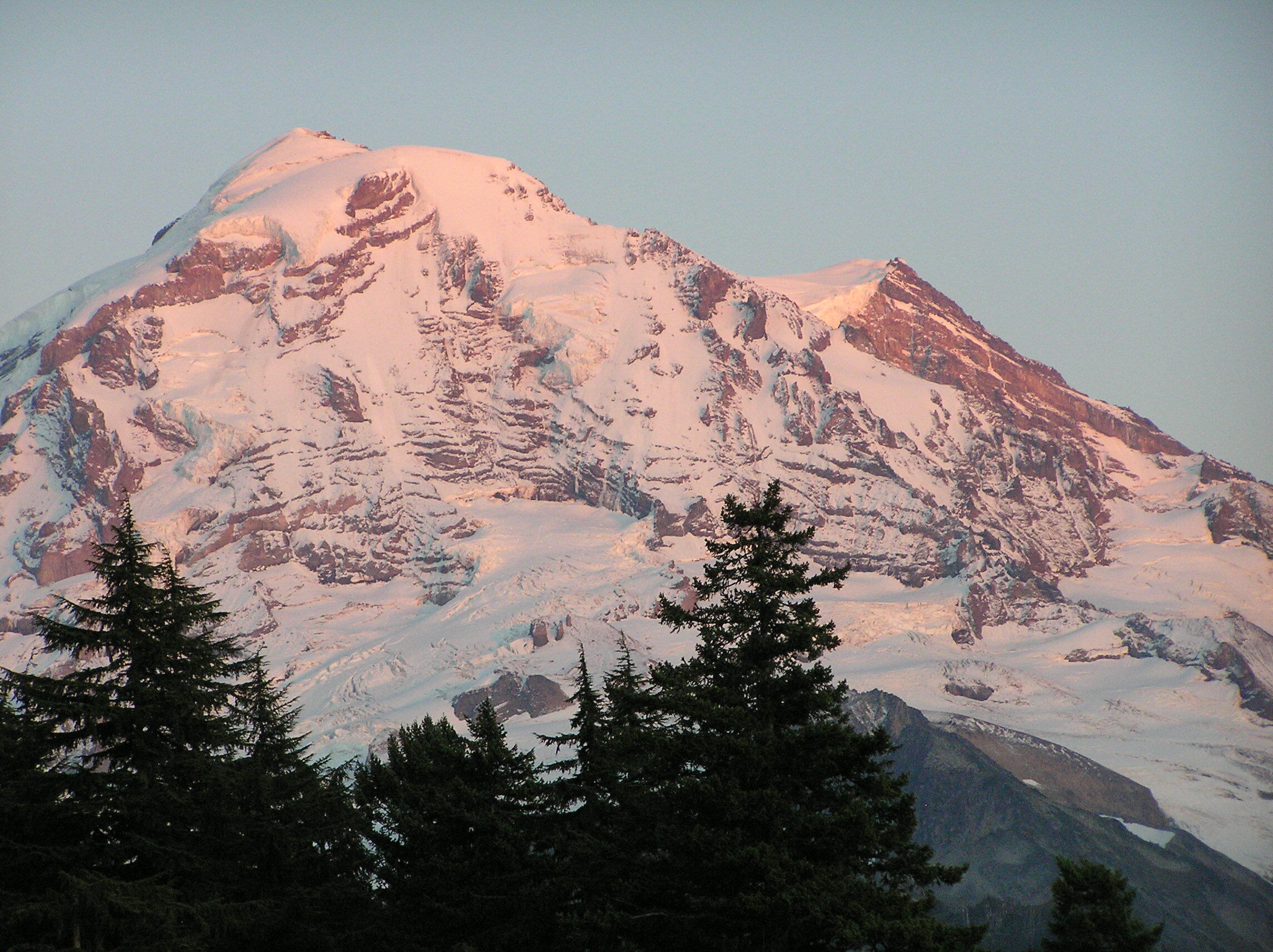
Climate change is altering summits of the tallest ice-capped mountains in the contiguous United States.
A new study by Scott Hotaling from the Quinney College of Agriculture and Natural Resources and Eric Gilbertson from Seattle University used differential GNSS measurements, satellite data, laser measurements and historical photographs to document the ways ice-capped summits in the Western United States are being affected by climate change.
For the last century, there have been five ice-capped summits in the contiguous United States, all in Washington State. The researchers measured the current elevations of the summits and compared their findings to historical surveys and photographs to assess whether their elevations have changed and whether their ice caps are still intact.
For Mount Rainier, Columbia Crest is no longer its highest point. The new summit is now rock on the mountain’s southwest rim roughly 133 meters away. All five of the historically ice-capped summits have shrunk since 1980, with four of the five shrinking by at least 6 meters (20 feet) from loss of snow and ice.
As of 2024, only two of the five summits still had perennial ice as their highest point. Free-air temperatures for the ice-capped summits indicate significant late summer warming of 2.75°C since 1950 and increases in summer melt days, with most of the change occurring since the late 1990s.
“Given the synchronous trends, we offer climate-induced loss of summit ice as the most likely explanation for the observed changes to ice-capped summits in the western United States,” the researchers write in their study.
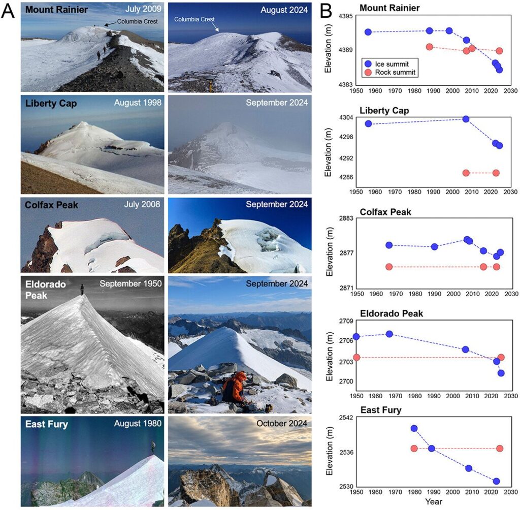
(A) Historical (left) and contemporary (right) photographs for each ice-capped summit included in this study. (B) Elevation over time for each ice-capped summit (blue) and the nearest rocky summit (red). (Image: Study authors)
The main GNSS survey tool used was a Spectra ProMark 220 dGNSS equipped with an Ashtech antenna. GNSS measurements of the ice-capped summits hads an accuracy of ±0.03 meters. For each dGNSS survey, the researchers recorded a 1-hour measurement on the ice-capped summit. If a nearby rock summit was at a similar elevation to the ice-capped summit, a 1-hour measurement was also recorded for it.
Korea will build its own navigation satellite system by 2034, providing independent positioning and navigation signals over an area spanning a 1,000-kilometer radius from the country’s capital, Seoul.
The Ministry of Science and information and communications technology (ICT) announced that it would finalize a plan for the Korean Positioning System (KPS) at a Space Committee meeting on Feb. 5.
According to a preliminary statement from the Ministry of Science and ICT, the KPS initiative will develop a ground test in 2021, core satellite navigation technology by 2022 and begin actual satellite production in 2024. The system will comprise a total of seven navigation satellites, three of them geostationary above the Korean Peninsula.
Figure from the 2016 paper shows a conceptual view of real-time WADGPS operation. The reference station transmits observation data at 1 Hz frequency to the master station. The master station is operated in real time and creates correction information and basic integrity information thereby configuring a message. A message is sent to the satellite communication simulation device according to its own transmission protocol. The satellite communication simulation device performs broadcasting of WADGPS correction information into the L1 band. A message created in every sec is coded with reserved GPS PRN C/A code and modulated with L1 frequency. Since additional correction information transmission medium such as geostationary orbit satellite or pseudolite is not considered in this study, radio frequency (RF) signals are created using simulation devices and performance was verified while connecting the signal with user receivers via cable. Additionally, a commercial communication network was used to transfer correction messages in order to verify user performance, which is located remotely. (Image: Korean Journal of Positioning, Navigation, and Timing)
Korea currently relies on the U.S. GPS system, which has suffered repeated local area jamming emanating from North Korea.
“As the GPS becomes a necessity in everyday life, broken signals for any reason can set off a nationwide chaos,” said an official for satellite navigation at the Korea Aerospace Research Institute (KARI).
Officials stated the the KPS will also improve available un-aided accuracy of GPS in its service area from about 10 meters now to less than one meter.
“Advanced nations are trying to secure strong GPS capabilities by sending up satellites to prevent a chaos that can take place while they depend on other nations’ satellites,” stated the KARI spokesperson.
The initiative appears to be separate from the Korean Wide Area Differential GPS System, whose development was the subject of a 2011 paper presented at the Institute of Navigation (ION) International Technical Meeting. The abstract for that paper stated:
“[The] project is scheduled for 2010 to 2014 under the contract with the Ministry of Land, Transport and Maritime affairs (MLTM). After that, Korea will launch a geostationary multifunctional satellite with a navigation payload which will be broadcasting augmenting signals for GPS.”
In March 2016, the Korean Journal of Positioning, Navigation, and Timing published a paper titled “Performance Analysis of WADGPS System for Improving Positioning Accuracy,” by Hyoungmin So , Jaegyu Jang, Kihoon Lee, unpyo Park and Kiwon Song. Its conclusion section stated:
“In this paper, configuration of observation reference stations and master station and initial experiment results were presented to verify accuracy correction performance of the WADGPS. The wide area correction algorithm was implemented using eight reference stations and one master station. For the initial performance verification, static and dynamic experiments were conducted. The experiment result showed that the static experiment had a horizontal accuracy performance with a level of 1 m (95 percent). In the dynamic experiment using a vehicle, performance degradation occurred compared to that of static experiment. The reason for this was due to the measured value error at the user receiver caused by multipath and visibility limitation. In summary, the implementation and performance of the algorithm of early stage were verified. For the future study, user operation characteristics will be considered and additional performance analysis on created correction information will be conducted.”
Everyone talks about the weather, but nobody does anything about it — right?
Our lead authors this month are doing something about it.
The July cover story of GPS World magazine was titled “See into the Smoke with Inertial.” This month’s feature could have been called “See into the Fog with CDGNSS,” but we just didn’t have room in the already extensive article to go into that angle. So here it is.
Precise carrier-phase differential GNSS positioning will in the near future become a must-have complement to cameras and lidar for all-weather automated driving. Positioning will be furnished, as the article explains, by a dense reference network broadcasting to low-cost antennas for precise (10 centimeter) performance.
Here’s the kicker, not included in your cover-story package, although hinted at by the orange and green trapezoids on the cover, and replicated in the fog-bound version above.
Such vehicle positioning would enable new driver-assistance systems. With precise knowledge of a vehicle’s position and orientation, intuitive driving directions can be rendered on the windshield in luminous paths that appear to be painted on the roadway. These paths will guide the driver along the fastest route to destination. Other symbols will suggest lane changes for safety or efficiency, and highlight the presence of vehicles dangerously close ahead. Because satellite navigation signals are not affected by rain, snow or fog, they can be combined with radar sensors to safely guide a driver or an automated vehicle in all weather.
As author Todd Humphreys explains it, “Imagine how relaxing it would be to follow a yellow brick road safely home! I envisioned this augmented-reality heads-up display during a recent road trip. Driving on unfamiliar roads, I was trying to interpret various route options on my wife’s smartphone while simultaneously fielding questions (in Spanish!) from my in-laws, and more questions from my nine-year old son. It was too much to ask of one driver!”
Not any more. That is, soon, in our brave new future, no longer.
A dense reference network facilitates low-cost carrier-phase differential GNSS positioning with rapid integer-ambiguity resolution. This could enable precise lane-keeping for automated vehicles in all weather conditions.
Strong demand for low-cost precise positioning exists in the mass market. Carrier-phase differential GNSS (CDGNSS) positioning, accurate to within a few centimeters even on a moving platform, would satisfy this demand were its cost significantly reduced. Low-cost CDGNSS would be a key enabler for many demanding consumer applications.
Centimeter-accurate positioning by CDGNSS has been perfected over the past two decades for applications in geodesy, precision agriculture, surveying and machine control. But mass-market adoption of this technology will demand much lower user cost — by a factor of 10 to 100 — yet still require rapid and accurate position fixing. To reduce cost, mass-market CDGNSS-capable receivers will have to make do with inexpensive, low-quality antennas whose multipath rejection and phase center stability are inferior to those of antennas typically used for CDGNSS.
Moreover, there will be a strong incentive to use single-frequency receivers, whereas almost all receivers used for CDGNSS in surveying and similar applications are multi-frequency. Despite these user-side disadvantages, mass-market precise positioning will be expected to demonstrate convergence and accuracy performance rivaling that of the most demanding current precise positioning applications: Users will be dissatisfied with techniques requiring more than a few tens of seconds to converge to a reliable sub-decimeter solution.
Meeting this challenge calls for innovation targeting both the rover (user) equipment and the reference network. Here we examine the challenge from the point of view of the reference network and offer demonstration results for a low-cost end-to-end system.
The recent trend in precise satellite-based positioning has been toward precise point positioning (PPP), whose primary virtue is the sparsity of its reference network. But standard PPP requires several tens of minutes or more to converge to a sub-10-centimeter 95 percent horizontal accuracy. Faster convergence can be achieved by recasting the PPP problem as one of relative positioning, thereby exposing integer ambiguities to the end user.
This technique, known as PPP-RTK or PPP-AR, is mathematically similar to traditional network real-time kinematic (NRTK) positioning. As the network density is increased, sub-minute or even instantaneous convergence is possible with dual-frequency high-quality receivers. Even single-frequency PPP-RTK is possible, with convergence times of approximately 5 minutes for a 40-kilometer network spacing.
For PPP-RTK and NRTK, convergence time is synonymous with the time required to resolve the integer ambiguities that arise in double-difference (DD) carrier-phase measurements, referred to here as time to ambiguity resolution, or TAR. As reference networks become denser, they can better compensate for spatially-correlated variations in signal delay introduced by irregularities in the ionosphere and, to a lesser extent, in the neutral atmosphere. Improvement is manifest as reduced uncertainty in the atmospheric corrections that the network sends to the user. Reduced uncertainty in the atmospheric corrections is key to reducing TAR.
Prior work has established an analytical connection between uncertainty in the ionospheric corrections (denoted σi ) and TAR. The existing literature does not, however, offer a satisfactory model for the dependence of σι on network density.
The prevailing model is based on single-baseline CDGNSS, which is inapt for PPP-RTK and NRTK. Moreover, prior work does not address the effect of network-side multipath on the accuracy of the corrections data, which becomes increasingly important as low-cost and poorly-sited reference stations are used to densify the network.
Here, we examine the relationship between ionospheric uncertainty and probability of correct ambiguity resolution, and present the results of an empirical investigation of the relationship between network density and the total uncertainty in network correction data. We developed a simple analytical model relating error variance in network corrections to network density. Our analysis and experiments indicate that for rapid TAR in challenging urban environments with low-cost receivers, network density must be significantly increased. We report on the design and deployment of a dense network in Austin, Texas, and demonstrate a new system that taps into the network to provide reliable vehicle lane-departure warning.
AMBIGUITY RESOLUTION
Reducing the ionospheric uncertainty σι allows a strong prior constraint to be applied in the ionosphere-weighted model, thereby increasing P( = z), the probability that the estimated and true integer ambiguity vectors are equivalent. It is instructive to consider single-epoch ambiguity resolution (AR), for two reasons.
First, for stationary users with low-cost equipment, multipath errors dominate in the carrier-phase measurement and are strongly correlated over 100 seconds or more. Thus, if single-epoch AR fails then a static user may have to wait an unacceptably long time for multipath errors to decorrelate enough to permit AR. In any case, singe-epoch performance is a strong predictor of multi-epoch performance over an interval short enough (a few tens of seconds) to satisfy impatient mass-market users.
Second, a convenient and accurate analytical model (by Dennis Odijk and PJG Teunissen) for single-epoch AR reveals the dependency of P( = z) on scenario parameters of practical interest: the standard deviation of ionospheric correction errors, the number of visible satellites, the standard deviation of undifferenced carrier- and code-phase measurement errors (including multipath-induced errors), a satellite geometry factor, the number p of free parameters to be estimated (p=3 for negligible tropospheric error, p=4 to estimate a single additional tropospheric parameter), and the number of carrier frequencies broadcast by each of the satellites (1, 2 or 3) along with each carrier’s wavelength.
The model is highly accurate for single-epoch AR, but only approximate for multiple epochs, with accuracy degrading as the data interval lengthens. The model’s inaccuracy results from its assumption that overhead satellites remain static from epoch to epoch, which yields pessimistic results for even fairly short data capture intervals (for example, 30 seconds). Fully accounting for satellite motion in an analytical model for P( = z) is an open problem, which is why studies that wish to account for satellite motion resort to simulation.
Figures 1 and 2 show single-epoch, single-frequency results from the analytical P( = z) model for parameters approximately reflecting the mass-market use case. The most important conclusion to draw from these figures is that for single-epoch, single-frequency AR to be even moderately reliable (PT⩾0.9) over the next few years, the ionospheric uncertainty σι must be held under 2 millimeters. This will relax somewhat as more Galileo and MEO BeiDou satellites come online, but signal blockage in built-up areas will raise the effective elevation mask angle significantly above the 15 degrees assumed here, reducing the number of available satellites. Thus, sub-2-mm ionospheric uncertainty remains desirable for urban environments even as GNSS constellations become fully populated.
Figure 1. Single-epoch single-frequency ambiguity fixing. Blue traces (left axis) indicate the probability P(z^=z) of correctly resolving all integer ambiguities with a single epoch of data as a function of the number of satellites m. Each trace represents P(z^=z) for a different value of ionospheric uncertainty σι. Green bars (right axis) represent the probability mass function P(m) for the number of satellites above an elevation mask angle of 15 degrees, assuming 31 GPS, 14 Galileo, and 3 WAAS satellites (projected mid 2017). Each blue trace is marked with the total probability of correct integer resolution PT, a function of both the trace itself and P(m). Other parameters of the scenario: geometry factor fg=2.5, standard deviation of undifferenced phase measurements σϕ=3mm, standard deviation of undifferenced pseudorange measurements σρ=50cm, and number of estimated parameters p=3.
Figure 2 . Total probability of a correct fix for the scenario of Figure 1 as a function of ionospheric uncertainty σι.
Figures 3 and 4 offer results for a dual-frequency (L1-L2) single-epoch scenario. All other scenario parameters are held as for the single-frequency scenario except that, in an attempt to be somewhat more pessimistic, P(m) is based only on GPS satellites. It is assumed that from each satellite the user can extract dual-frequency measurements. As with the single-frequency case, it is evident that dual-frequency PT is strongly dependent on σι. The dual-frequency case is more forgiving, but substantial performance improvement can still be had by reducing σι to under 2 mm.
Figure 3. As Figure 1 except for dual-frequency (L1-L2) measurements and the probability mass function P(m) corresponds only to a constellation of 31 GPS satellites. The elevation mask angle is again taken to be 15 degrees. It is assumed that dual-frequency measurements can be obtained from every GPS satellite.
Figure 4. Total probability of a correct fix for the scenario of Figure 3 as a function of ionospheric uncertainty σι.
Corrections Uncertainty and Network Density. A key question arises in connection with σi: How is related to reference network density? One expects to decrease with increased network density, but what is the exact relationship?
Dennis Odijk’s work adopts a linear relationship between σi and the distance l between the user and the nearest reference station:
σi = βl, 0.3 ≤ β ≤ 3 mm/km
Parameter β depends on ionospheric activity; Odijk recommends determining β empirically. Similarly, his other work adopts a linear relation, with β = mm/km. But there appears to be no justification for applying this linear model to ionospheric corrections provided to a user by a network of reference receivers. The linear trend corresponds to individual single-baseline solutions involving a single master reference station without network aiding; it is not representative of how σi varies for a rover within a reference network.
Instead of determining how σi varies throughout a reference network, it will be more useful to consider the spatial variation in the variance of aggregate error in network-provided corrections. The aggregate error variance, denoted , can be modeled as the sum of variances associated with (1) residual ionospheric delay error, (2) residual neutral atmospheric (hereafter tropospheric) error, and (3) error due to carrier-phase multipath at the reference network stations:
This model assumes that precise orbital ephemerides are used to eliminate spatially-correlated errors due to satellite ephemeris errors and that the contribution to from reference station carrier-phase thermal noise is negligible compared to reference station carrier-phase multipath error.
Focusing therefore on σv , consider its relationship to reference network density γ, expressed in stations per unit area. This relationship depends on the assumed model for the DD ionospheric and tropospheric delays. Let a denote the master reference station and let S = {s1, s2, …, sN} denote the set of all secondary stations available in the network. Then, for pivot satellite i and alternate satellite j , suppose that the true combined DD atmospheric delay at secondary station s∈S can be accurately modeled as follows, where xs, ys, and zs represent the secondary station’s east, north, and up displacement from the master: (1)
Dai et al. refer to this model as a linear interpolation model or first-order surface model. The quantities and are the model parameters for the satellite pair i, j.
Map showing trends in σv across a simulated reference network assuming a linear model for combined DD ionospheric and tropospheric delays and independent errors due to multipath at each station. The master station is marked in black; secondary reference stations are marked in white. Blue denotes low σv. Red denotes high σv.
For the linear model in (1), one can show that if stations are sufficiently uniformly distributed (i.e., no station clumping), then the average value of σv across a network, denoted , is approximately related to the network density γ by (3)
where q is a parameter related to the variance of the uncorrelated errors , s∈S. This approximation becomes highly accurate as γ increases. [See full paper for details.]
It is clear from (3) that, for the linear model (1),can be driven to an arbitrarily small value by increasing the network density γ, and this is true despite the presence of multipath in the reference station carrier-phase measurements. Whether (3) applies in practice depends on whether (1) can be considered an accurate model for , at least over a compact region. The following section examines this question empirically. It further seeks to identify, for an example dense reference network, the density γ beyond which further reduction inno longer matters (would no longer improve ) because rover multipath dominates.
ANALYSIS OF A DENSE REFERENCE NETWORK
We examined σι as a function of network density using data from several organizations providing GNSS reference station observations: National Geodetic Survey Continuously Operating Reference Stations, UNAVCO, and the California Real Time Network. This combination allowed analysis of a hypothetical reference network of 23 high-quality GNSS receivers with an overall network density of approximately 8 nodes/1,000 km2, or an average inter-station spacing of 14 km. The relative positions of the sites selected to comprise this reference network, located between Los Angeles and Pomona, California, are depicted graphically below.
Depiction of the placement of the 23 GNSS reference stations. Horizontal positions are relative to the master station, LONG of CRTN, in kilometers. The color map indicates the height of each station above the WGS 84 geoid in meters.
DD carrier-phase observations from GPS L1 C/A signals spanning GPS weeks 1850 through 1859 were used for the analysis. A minimum satellite elevation mask was enforced at 20 degrees. Any satellite not above the elevation mask and providing carrier-phase observations at both the beginning and end of each processing window was excluded. A step size of 10 minutes was used. The longest available sub-window, meeting the above requirements and providing a minimum of 6 satellite vehicles (1 pivot satellite and 5 others), was selected for processing.
To facilitate batch processing, integer ambiguities were assumed to be resolved correctly when the mean standard deviation of carrier-phase residuals for that solution was less than one quarter wavelength of the GPS L1 frequency. In application, this constraint resulted in rejecting only 0.6 percent of all solutions.
Network Corrections Estimation. Estimation of network corrections made use of least-squares estimation applied to carrier-phase residuals measured between master station LONG, denoted a hereafter, and secondary reference stations s∈S, where S is now taken to be the set of all stations other than LONG. Consider the following model for the DD carrier-phase measurement, expressed in meters, between master station a, secondary station s∈S, pivot satellite i, and alternate satellite j:
(4)
Here, λ is the carrier wavelength; is the DD carrier-phase measurement, in cycles; is the DD range; is the DD integer ambiguity; is the DD combined atmospheric delay, which includes tropospheric and ionospheric delays; and is the DD carrier-phase measurement error, which is dominated by carrier-phase multipath error at a and s.
Experimental analysis ofas a function of network density proceeded as follows. A subset of secondary stations Sk ⊂S was chosen, together with a, to act as the kth test network. A large number K of subsets Sk of various geographic size and density were analyzed. Let {S\Sk} denote the set of secondary stations not in the kth test network. For each Sk, k = 1, 2,…, K, all secondary stations in {S\Sk} were designated, one at a time, to act as a test station, or rover. Atmospheric delays estimated by the kth network for test station s∈{S\Sk} were then differenced from actual delays measured by s to evaluate the quality of the atmospheric delay estimates.
Details of the atmospheric delay estimation procedure for the kth test network are as follows. For each s∈Sk, a DD measurement residual was formed for each pivot satellite i and alternate satellite j as
(5)
where was assumed known to sub-millimeter accuracy and was assumed to have been resolved correctly. The true DD atmospheric error contributing to (5) was assumed to vary linearly with geometry over sufficiently short baselines as modeled in (2). The DD multipath error term was assumed to be zero mean, and the component due solely to s was assumed to be uncorrelated with all corresponding components .
Under these assumptions, can readily be estimated via least squares. Let be the vector containing the residuals for |Sk|x1. This residuals vector can be modeled as
(6)
where H is an |Sk|x4 matrix whose rows are of the form [xs ys zs1]. The 4 x 1 vector contains the parameters of the hyper-plane to be estimated at each epoch. The |Sk|x1 vector wijcontains DD measurement errors.
An estimate from a least-squares solution of (6) was used to produce a network correction for a test secondary station s∈{S\Sk}, acting as rover, at location xs, ys, zs :
(7)
The subscript l on the atmospheric correction indicates that the correction is based on a linear model for DD atmospheric errors; it is used to distinguish the correction from those produced by a quadratic model later on. The correction was applied at test station s∈{S\Sk} to produce a corrected DD phase measurement
This procedure was repeated at each epoch for each satellite pair i, j visible to each test station s∈{S\Sk} of the kth test network, k = 1, 2,…K.
If the assumed models hold, then in the limit as the network density increases, can be modeled as
(8)
where is DD phase measurement error due only to multipath at s. In other words, as network density increases, application of the network correction eliminates not onlybut also , the component of the DD phase measurement error due to multipath at the master.
Linear least-squares compared to quadratic-least squares estimation. To evaluate the assumption that DD tropospheric and ionospheric errors vary proportional to relative position, c1 was estimated with the full set of secondary stations S for single epochs at 300 second intervals. The probability distributions of the contributions of those parameters (e.g., cxlxs and not simply cxl) are shown below. For comparison, equivalent values are calculated for a quadratic least-squares estimate of the following form:
(9)
Here, the subscript q of denotes a quadratic model for DD atmospheric delays. The distributions of comparable terms from (9) are also shown in the next two figures. These data represent the collection of all satellites above the elevation mask angle. It is noted that when all satellites are considered together, the expected value of these terms is very near zero.
Probability densities of the terms estimated at the station location for SPMS of UNAVCO. As indicated by the legend, the linear components are shown for a linear least-squares estimation as well as the linear components for a quadratic least-squares estimation. These data represent the probability densities for all GPS satellites combined.
Probability densities of the terms calculated at the station location for SPMS of UNAVCO.
The next two figures show the same data as the two above, but with each GPS satellite plotted separately. It is noted that the linear parameters, when considering only a particular satellite, are not necessarily zero-mean. This is hypothesized to be a manifestation of the satellite orbit reflected in the tropospheric and ionospheric errors. It is interesting to note that the quadratic terms shown in the second figure below largely exhibit zero mean behavior despite non-zero mean for the associated linear terms.
Probability densities of the terms for every GPS satellite observed, calculated at the station location for SPMS of UNAVCO, where each plot line represents a different GPS satellite. This figure is intended to qualitatively illustrate the non-zero mean nature of these linear terms when considered for individual satellites.
Probability densities of the terms for every GPS satellite observed, calculated at the station location for SPMS of UNAVCO, where each plot line represents a different GPS satellite. This figure is included to qualitatively illustrate the largely zero mean nature of these quadratic terms when considered for individual satellites.
Probability densities of the difference between linear least-squares and quadratic least-squares network correction estimates for representative reference stations. The red vertical lines denote boundaries between which 68.27% of the probability distribution is contained; displayed as a comparative proxy to lσ of the Gaussian-distribution (these distributions are non-Gaussian). Recall that CGDM has a distance to the master station of 15.1km, BGIS is at 21.6km, and LORS is at 23.1km.
The figure above shows the probability distributions of the difference between (7) and (9) (i.e., ) at three representative reference station positions. It can be noticed that despite the increasing baseline distance of LORS and BGIS as compared to CGDM, there is no apparent correlation in these estimation errors. Notice that CGDM and LORS have very similar distributions despite their difference in baselines. BGIS and LORS, with similar baselines, exhibit very different distributions. There is no apparent correlation found between reference station positions and these error terms. Additionally, these distributions are zero-mean for all s∈S (to within 0.5 mm in each case) with 68.27% boundaries positioned between 1.5-5.5 mm. Because these errors appear indistinguishable from multipath, it is concluded, for this specific network and time period, that linear least-squares estimation is sufficient for estimating tropospheric and ionospheric errors. This is fortunate, because the linear model for atmospheric DD delays provides an averaging effect on multipath present at the reference stations which minimizes the introduction of multipath errors into the estimates produced.
Uncorrected carrier-phase residuals. The figure below shows the expected values for DD carrier-phase residual standard deviations for all s∈S through use of uncorrected observations. These data were produced by averaging the standard deviation of the DD carrier-phase residuals calculated at each epoch across all satellites present in the solution. The fitted curve indicates a linear growth of DD carrier-phase residuals with β = 0.62 mm/km. Additionally, the mm-level scatter of these data points suggest that position biases of the resolved reference station positions are also mm-level. If the linear fit is shifted down by approximately 4 mm (e.g., taking the minimum data points as those with very little position bias) and extrapolated to 0 km, one can consider this as providing a rough estimate of DD multipath at the reference stations; 4.7 mm (DD) or 3.3 mm (single-difference equivalent).
Standard deviation of uncorrected DD carrier-phase residuals versus baseline distance between each of the 22 reference stations and the master reference station.
Uncorrected Carrier-Phase Residuals. Figure 5 shows the expected values for DD carrier-phase residual standard deviations for all secondary stations, based on observations that were not corrected for atmospheric delay. These data were produced by averaging the standard deviation of the DD carrier-phase residuals calculated at each epoch across all satellites present in the solution. The fitted curve indicates a linear growth of DD carrier-phase residuals with distance to the master. The mm-level scatter of these data points suggest that biases of the resolved reference station positions are also mm-level.
Figure 5. Standard deviation of uncorrected DD carrier-phase residuals versus baseline distance between each of the 22 reference stations and the master reference station.
Network-Corrected Residuals. Figure 6 displays similar data to Figure 5, except that the carrier-phase residuals are those that remain after network corrections are applied. Each data point corresponds to a particular subset of secondary stations together with the master, and a particular rover selected at random from the remaining stations. Both the size and specific selection of secondary stations comprising each subset were randomly selected. In all, 70 different network configurations and more than 3.67 million NRTK solutions were analyzed.
Figure 6. Standard deviation of carrier-phase residual remainders (the carrier-phase residuals which remain after application of network corrections) versus average network density. The fitted curve is simply a polynomial fit of these data; it is not based on any theoretically anticipated behavior.
Figure 6 shows that carrier-phase residuals after application of network corrections are considerably reduced compared to those original magnitudes seen in Figure 5. With increasing network density, the DD residuals’ deviation asymptotically approaches a minimum value of about 4 mm, which corresponds to an undifferenced deviation of 2 mm. This floor is due to multipath at the rover. Deviations in excess of this floor are caused by residual ionospheric errors and, to a lesser extent, neutral atmospheric errors.Attributing the excess deviation entirely to residual ionospheric errors, and assuming these are uncorrelated with multipath, one can estimate from Figure 6 the undifferenced ionospheric uncertainty. For example, for a 50-km inter-station distance, σι=(℘(142 – 42))/2=6.7mm. To achieve the σι<2 mm recommended earlier for fast and reliable AR, station separation should be no more than 22 km, which we round down to a recommended value of 20 km to provide a margin of station redundancy.
NETWORK DEPLOYMENT
We have developed and deployed a low-cost reference network testbed in Austin, Texas, with site hosting courtesy of the Texas Department of Transportation. The Longhorn Reference Network boasts a dozen stations, with plans for 20 (Figure 7). The network’s average inter-station spacing is far shorter than the 20-km spacing recommended earlier. The tighter spacing provides redundancy and flexibility of experimentation. The low-cost reference stations are deployed in environments with greater multipath and signal blockage than those of the high-quality stations studied earlier. Such non-ideal signal environments are to be expected in a dense low-cost reference network, for which choice of station siting is driven largely by opportunity.
Figure 7. Overview of the planned Austin area reference network (Google Maps).
The reference station design, pictured in Figure 8 and diagrammed in Figure 9, is novel. Each station is a self-contained, solar-powered node supporting a software-defined dual-frequency, dual-antenna GNSS receiver with an always-on cellular connection to university servers for data collection and software maintenance.
Figure 8. Low-cost reference station in the Longhorn Reference Network.
Figure 9. Reference station components.
Live Vehicle Demonstration. In partnership with Radiosense, an Austin-based precise positioning startup, we have developed and demonstrated a low-cost vehicle lane departure warning system that receives corrections from our dense reference network. The system takes in lane widths from an external database and infers a safe driving corridor within each lane by analyzing the behavior of human drivers on the same road. A vehicle’s proximity to the lane boundary is displayed in real time to the driver and passengers.
For robustness against cycle slips and to provide a baseline against which to compare future improvements, the system currently employs single-epoch CDGNSS positioning without aiding from additional sensors. In choosing a single-epoch approach, the system naively discards information regarding the underlying integer ambiguities at the beginning of each measurement epoch. Still, the system performs well with the typical number of overhead signals in a light urban environment: correct and internally-validated solutions were available in over 92 percent of measurement epochs. When a second rover antenna is included to combat multipath with spatial diversity, this percentage improves to 96. Such good single-epoch performance suggests that, when armed with additional sensor aiding and proper integer ambiguity persistence, reliable and accurate vehicle positioning can be maintained in more challenging environments.
Demonstration setup. The live demonstration followed a predetermined route in the vicinity of the University of Texas campus. The 1-mile route (Figure 10) passed through both open-sky and partially-blocked environments.
Figure 10. Demonstration route.
Prior to the demonstration, the vehicle was driven several times on the same route collecting GNSS measurements to precisely map typical driving trajectories on the route. The ensemble of trajectories was used to build a centimeter-accurate model of the lane center along the route. The sensing equipment employed during this mapping phase is no different than that used during the demonstration, making feasible eventual crowd-sourcing, wherein end-user vehicles generate and update the centerline models.
The demonstration vehicle was outfitted with two dual-frequency GNSS antennas mounted with magnetic bases onto the roof. The first antenna, designated primary, operated as the rover in a single-baseline CDGNSS solution against the master reference station of the Longhorn Reference Network, as illustrated in Figure 11. This baseline provided the geo-referenced, centimeter-accurate vehicle position. The other antenna, designated secondary, was paired with the primary antenna to produce a constrained-baseline CDGNSS solution providing sub-degree-accurate vehicle heading. The secondary antenna also served as a backup when the primary antenna produced a result that did not pass the precise positioning engine’s internal validity testing.
Figure 11. GNSS antenna configuration. A single-baseline precise position solution between the primary antenna and the master reference station provides precise vehicle position. A constrained-baseline 2D attitude solution between the primary and secondary antennas provides heading.
The GNSS antennas were connected to a low-cost, dual-frequency front-end in the trunk of the vehicle (FIGURE 12)which downconverted and digitized the incoming signals and subsequently fed them to a low-cost single-board computer running the precise positioning engine. A cellular modem received real-time measurements from the master reference station, while a WiFi router streamed real-time solutions to several Android devices in the vehicle for real-time visualization of precise within-lane position.
Figure 12. Low-cost, dual-frequency rover system in the trunk of the vehicle.
Demonstration Results. Figures 13, 14 and 15 show snapshots of the Android application and a still frame of the side of the vehicle in three different scenarios. The large rectangle indicates vehicle position with respect to the modeled lane center, changing color from green, when the vehicle is within the safe driving corridor, to yellow as the vehicle nears the edge of the lane, and finally to red if the vehicle breaks the lane boundary. One could imagine wrapping a control loop around these signals to enable last-moment lane-keeping.
Figure 13. Vehicle position relative to lane edge (left) synchronized in time with video still frame (right), centered safely within the lane, as depicted by green rectangle.
Figure 14. Vehicle nearing lane edge, as depicted by yellow rectangle.
Figure 15. Vehicle crossing lane edge, as depicted by red rectangle.
Figure 16 reveals the precision with which the positioning engine was able to locate the vehicle’s driver-side antenna in four repeated passes along the test route. The variation between the four yellow traces is primarily due to driver non-repeatability; actual measurement precision is at the centimeter scale. A small bias in the traces’ registration to the picture is present because Google Earth imagery is only registered to the International Terrestrial Reference Frame with meter-level accuracy.
Figure 16. Four repeated traces of driver’s side antenna as vehicle made a turn.
Figure 17 shows a time history of the vertical deviation from the route mean, in meters. The zoomed view of the vertical deviation shown in Figure 18 allows one to appreciate the precision of the positioning engine: the vertical trajectory is smooth at the centimeter level. Figure 19 shows the DD residuals in carrier phase and pseudorange for GPS PRN 30 during the four loops in Figure 17. One-sigma undifferenced phase and pseudorange deviations are 3.4 mm and 42 cm, respectively.
Figure 17. Time history of the vertical deviation from the route mean, in meters.
Figure 18. Zoomed view of the time history of the vertical deviation from the route mean, showing the centimeter-level precision in the 3.3 Hz positioning data.
Figure 19. Double-difference carrier phase (top) and pseudorange (bottom) residuals for GPS satellite 30 at frequency L1 over the full time interval shown in Figure 17.
The figures demonstrate that the precise positioning engine fed by reference data from the Longhorn Reference Network maintained centimeter-accurate knowledge of the vehicle’s position during almost the entire trajectory, despite passing between a large football stadium and parking garage, each of which introduced significant signal blockage and multipath.
For the data shown in Figure 17, 96 percent of the 3.3-Hz measurement epochs resulted in a correct and internally-validated positioning solution. The majority of the remaining solutions were correct but did not pass internal validation. For only 0.6 percent of solutions were the carrier-phase integer ambiguities resolved incorrectly, but all of these incorrect solutions were caught and excluded by the validation algorithm.
Furthermore, the number of overhead signals during the time in which this particular dataset (set A) was taken was average, as seen in the upper plot of Figure 20. 16 signals above 15 degrees elevation were available during this time. In contrast, the number of overhead signals for a second dataset taken 8 days prior (set B) was much worse, with only 12 signals above 15 degrees elevation, as seen in the lower plot.
Figure 20. The number of signals above a 15-degree elevation mask. Each plot spans an entire day. The black arrows denote the time of day in which two different datasets, A and B, were taken. The dashed red line represents the mean number of signals above the mask over both days. Dataset A was taken during a nominal time when 16 signals were available, while dataset B was taken during a worst-case time when only 12 signals were available.
For insight into the performance of the positioning engine as a function of the number of overhead satellites, Table 1 details the performance of these two datasets (as well as a third dataset) in terms of the percentage of epochs that passed the positioning engine’s internal validation testing, based on a ratio test with a fixed threshold of 2.0. Results are shown for single- and dual-antenna positioning solutions and for dual-antenna vehicle heading solutions.
Table 1. The performance of each dataset in terms of the percentage of solutions that passed validation testing.
A large drop-off in positioning performance occurs when the number of overhead signals is reduced below 16, while the constrained-baseline heading determination performance remains good throughout. Fortunately, it will not be long until even more signals are available. Within the next 8 months, the Galileo constellation will add six fully operational satellites. These will bring the number of GPS L1, GPS L2C, Galileo E1, and SBAS signals that are above 15 degrees elevation to 16 or more 95 percent of the time, enabling high-reliability single-epoch CDGNSS positioning.
CONCLUSIONS
For a sufficiently dense reference network, linear least squares estimation can be applied to the task of reducing uncertainties due to tropospheric and ionospheric delays for the purposes of providing improved positioning accuracy as well as faster time to ambiguity resolution for carrier-phase differential positioning. High network density allows use of a strong linear model for atmospheric delays, which has the virtue of suppressing network-side multipath errors in the provided corrections.
A network of 23 high-quality reference stations in the vicinity of Los Angeles, California, was studied to determine what network density is sufficient to make all network-side error sources negligible compared to rover receiver multipath. A density of three stations per 1,000km2, or an average inter-station spacing of 20 km, was found to drive network-side ionospheric, tropospheric, and multipath errors well below rover receiver multipath.
These findings motivate a significant densification of permanent reference networks, at least in built-up areas where signal blockage and multipath are common, to support mass-market applications for which low user (rover receiver) cost and rapid convergence to a reliable sub-decimeter position are a priority. In a light urban setting, and with the kind of satellite coverage that will soon become the norm, we demonstrated vehicle lane departure warning in a field test that produced highly reliable instantaneous sub-decimeter positioning.
ACKNOWLEDGMENTS
This work was supported in part by Samsung Research America, by the Data-Supported Transportation Operations and Planning Center (D-STOP), a Tier 1 USDOT University Transportation Center, and by the Texas Department of Transportation under the Connected Vehicle Problems, Challenges and Major Technologies project.
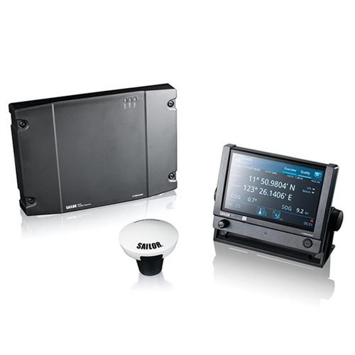
The Sailor 6560 GNSS System is delivered with the Sailor 6004 Control Panel and the corresponding Sailor 6285 GNSS Antenna or Sailor 6286 DGNSS Antenna.
Cobham SATCOM has launched two new Sailor satellite navigation receivers. Both the Sailor 656X GNSS and new Sailor 657X DGNSS (Differential GNSS) are black-box products designed to be part of a system Cobham SATCOM refers to as its “multi-function universe.”
The advanced touchscreen Sailor 6004 Control Panel at the heart of the Multi-Function Universe provides full control for all products connected to it from a single device. The Sailor 656X GNSS and Sailor 657X DGNSS join the Sailor 6391 Navtex and Sailor 628X AIS as new generation Sailor products designed to work with the Sailor 6004 Control Panel. Operation of all systems connected to the Sailor 6004 Control Panel is done by selecting the icon for the product on the touchscreen, providing access to set-up, functions and diagnostics.
“The Multi-Function Universe approach means that a variety of products can all be accessed from a single screen on the bridge and anywhere else a repeater is needed, making installation far more flexible than with traditional products that all require their own screen. The approach also saves space on the bridge, and importantly, makes the life of maintenance engineers easier as they have a single point of entry to the network,” explains Claus Hornbech, Business Manager, Cobham SATCOM.
The Sailor 656X GNSS and the Sailor 657X DGNSS collect satellite data from any available navigation satellites including GPS and GLONASS and distribute it to a variety of on board systems such as; ECDIS (Electronic Chart DISPlay System), INS (Integrated Navigation System), GMDSS (Global Maritime Distress & Safety System), SATCOM (Satellite Communication System), MCS (Master Clock Systems) and PABX (Telephone Exchanges).
Cobham SATCOM offers four variants of its new satellite navigation products, all of which are designed 100% in house. The Sailor 6560 GNSS System and Sailor 6570 DGNSS System are delivered with the Sailor 6004 Control Panel and the corresponding Sailor 6285 GNSS Antenna or Sailor 6286 DGNSS Antenna, while the Sailor 6561 GNSS Basic and Sailor 6571 DGNSS Basic are delivered with the antennas only.
All four variants use the same proprietary Sailor 6588 DGNSS Receiver, which provides highly accurate data, enhanced by means of Satellite Based Augmentation System (SBAS) from various areas including WAAS (Wide Area Augmentation System) for the United States, EGNOS (European Geostationary Navigation Overlay Service) in Europe, and systems from Japan, India and Russia. The Sailor 6285 GNSS Antenna and Sailor 6286 DGNSS Antenna are also both new, designed and manufactured according to Cobham SATCOM’s quality standards.
“The accuracy and availability of satellite positioning and timing data is vital to vessel safety as so many critical navigation and communication systems rely on it to operate,” adds Jan Kragh Michelsen, VP Maritime Business Development, Cobham SATCOM. “All elements, from the black-box to the antennas, multi-function display and the user-interface of the systems are new and developed 100 percent in house at Cobham SATCOM, so customers can be confident in the reliability of our new GNSS and DGNSS products, in addition to our revolutionary Multi-Function Universe operating concept.”
Differential GNSS+INS for Land Vehicle Autonomous Navigation Qualification
By Gilles Boime, Emmanuel Sicsik-Paré and John Fischer
Land-vehicle autonomous navigation requires centimeter-level qualification tools to enable confidence build-up for delivery to open-road traffic insertion. External positioning sensors over a dedicated road section can be replaced with an embedded high-accuracy, highly responsive epoch-by-epoch differential GNSS receiver coupled with an inertial navigation system. The demonstrated absolute accuracy and mobility extends the potential test area and minimizes cost for multi-environment validation.
Cover courtesy of Mercedes.
Personal cars and commercial trucks are continuously improving the driver experience and safety thanks to integration of more significant and machine-assisted control systems. Advanced driver-assistance systems (ADAS) are now integrated in all luxury cars and moving into mainstream products. Technologies covered by ADAS are specific for each car integrator, but increasingly they include now involving more safety features, such as driver assistance and partial delegation to autonomous control for small maneuvers such as lane control. The generation of ADAS systems introduced in early 2015 on high-end models are engaging more intelligence from the control system such as:
Lane departure warning system
Speed assistance and control
Driver assistance and control
Autonomous emergency braking.
It is not only individual drivers who want this technology, but also governments that are getting involved to prevent accidents and minimize the economic impact associated with them. In the European Union, the general safety regulation 2009/661 was the first step to engage member-states to act as a regulator to mandate car safety improvements. The European Transport Safety Council, a non-profit private association, released in March 2015 a position paper titled “Revision of the General Safety Regulation 2009/661.” It promotes the introduction of lifesaving technologies like intelligent speed assistance, autonomous emergency technology including all speed and pedestrian detection, and lane-departure warning systems as the next step of regulation.
Car manufacturers are not far behind. They understand their customers’ expectation of minimized risk and enhanced driving experience. Telematics is also a path to convert a single vehicle into a fully intelligent, connected and entertainment object with an associated high value. So every car manufacturer is willing to be seen as a technology master.
Toyota, for example, plans to integrate collision-prevention technology in all its mainstream and luxury cars by 2017. The ADAS new generation focuses on radar-activated cruise control technology for the collision-prevention system. The control system maintains distance from a vehicle ahead and can stop the car if driver doesn’t react. The next step is to monitor driver attention with sensors like cameras focusing on the driver’s eyes, and the pressure of the hand on the steering wheel.
However, no fully driverless car is expected in the next 10 years. This technology is limited by legal issues and the lack of reliable nationwide mapping data.
Since the technology must be fully proven to prevent any lethal threat on the user and other drivers, most car and truck companies are working actively on qualifying driverless technology today. Nissan began testing driver-assist technology on open-road traffic in Japan in late 2013. It enables highly advanced systems such as lane-keeping, automatic lane change, automatic exit, automatic overtaking of slower or stopped vehicles, automatic deceleration during congestion on freeways, and automatic stopping at red lights. This is a step towards attaining fully automatic driving, targeted for 2020 by Nissan.
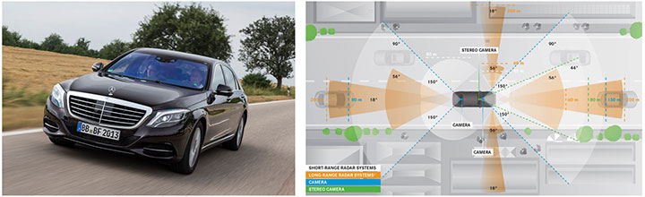
Some European manufacturers such as Daimler Benz are also early adopters. Daimler/Mercedes uses the Bertha Benz prototype car to test autonomous driving technologies. It merged multiple vision, radar and GPS sensor with digital map to monitor an open-road 100-kilometer trip in August 2013 (Figure 1).
Figure 1. Bertha Benz test car, left, running fully autonomous 103-kilometer trip in open road including 27 percent narrow urban roads. Right, networked sensor systems of the S 500 Intelligent Drive research vehicle.
All manufacturers are building driverless capability into their technology demonstration concept cars:
Mercedes with F 015 Luxury presented at the Consumer Electronic Show, early 2015;
Audi with Prologue, an extrapolation of test car RS7 concept equipped with SuperFast driverless pilot;
BMW’s electric i3 car is integrating ActiveAssist technology that enables portions of drive to be without any manual intervention, such as car parking and autonomous rally to a meeting point;
Google’s self-driving vehicle that conforms to California license requirements for driverless tests in open traffic;
Tesla model SD autonomous test car.
Although most market leaders agree that this is not a technology for mainstream production in the next few years, they all work very efficiently to master the technologies. It is a big challenge to integrate all the sensors and the navigation functions to autonomously and accurately position the vehicle on a map. The whole system must be certified to prevent any liability in case of a crash, a case that would engage the solution provider and the vehicle manufacturer.
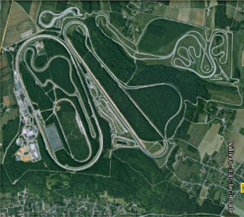
A large part of the qualification task will benefit from simulations and integration testing platforms in realistic conditions. At the very least, a very robust final open-space validation test must take place. Car manufacturers/integrators are using private test facilities in open air to perform serious trials before proceeding to real traffic conditions. Renault uses a 10-square-kilometer facility in France (Figure 2) to perform private tests in a protected area.
Figure 2. Renault outdoor test center at Aubevoye, France.
New autonomous car drive tests have mandated equipment enabling measurement of the car’s position on the track with an extremely high precision and repeatability. There are two competing technologies to do this:
Install many location sensors on the test track;
Use a general absolute positioning system.
Here we focus on an absolute positioning system that is affordable, easy to install and low maintenance. It is based on two main assertions:
The autonomous pilot can position accurately on the test track;
The test track is accurately referenced to the absolute positioning system.
We focus more closely in this article on the first assertion; the second one can be covered with a specific calibration trial where equipment, as discussed further, can be used in quasi-static mode and experience consistent accuracy. Let us have a deeper look at the candidate position technologies to verify autonomous pilot accuracy.
Positioning Technologies
Many technologies have been proposed to obtain vehicle position on the course. However, they all must be compatible with a reliable mapping database. Given the lack of consistent road infrastructure equipment with alternative capabilities, GNSS positioning is the sole enabling method to fit to a map every place around the world. That is why driverless systems always include a GNSS sensor to help other data matching with the map. The versatility and low cost of GNSS positioning makes it a candidate for open-air validation as well.
Standalone Standard Positioning Service GPS. The SPS single-frequency GPS receivers are included in so many nomadic appliances today that they are a commodity. Since their introduction 20 years ago, their performance is well understood. Some trials were performed in different area profiles with satellite constellation position dilution of precision (PDOP) < 2. Worse results were obtained from deep urban canyons in downtown Seattle, Wash.
For every technology, the relevant performance for the test course is the lateral error to the expected center of the lane in the two horizontal dimensions, referred to as 2D or N/E for orientation north and east.
For standalone SPS GPS, the lateral error standard deviation in 2D can be as high as 46 meters and have peak errors up to 660 meters. Lateral error in 3D can be as high as 20 meters with peak errors up to 175 meters.
Such performances are out of range for any positioning verification. It can only deliver a rough estimate of the point on the map, but would not provide tight correlation with other sensors for the navigation system.
Hybridized IMU and SPS GPS. Coupling of an absolute navigation GPS receiver with an inertial measurement unit (IMU) can mitigate corruption of the navigation solution when intermittent GPS signal outage is encountered. The hybrid approach is beneficial on any difficult signal transmission path from the satellite that is not line-of-sight: in urban canyons, deep foliage, under bridges, tunnels and in any multipath area. It also yields benefits in the very short term (less than a few seconds) for dispersion on the position computed from the sky.
Over the last 10 years, the combined benefits of micro-electro-mechanical sensors (MEMS) and tight coupling algorithms have raised the bar of positioning accuracy. It enables smoothed position along track and dead reckoning (DR) in case of GNSS signal outage.
Lateral error standard deviation in 2D is lowered to 2.3 meters and peak error up to 10 meters. However, this performance is still too poor to validate a vehicle position in the lane.
Hybrid Differential Single Frequency and IMU. The next step to mitigate systematic errors of the GNSS system is to use a set of multiple reference receivers in the vicinity of the area covering the test course. The reference receivers are static. The position of the reference is determined using long-term averages to mitigate constellation errors. A minimum for a position fix of 20 minutes is commonly reported. Then the position error standard deviation in 2D is less than 2 centimeters for baselines shorter than 100 kilometers.
For a MEMS integrated with a standard SPS GPS single-frequency receiver with DGPS correction on a mobile platform moving at less than 70 km/hour with HDOP < 1.4, Table 1 compares performance in a 2013 test.
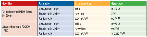
Table 1.IMU performance grades.
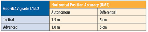
Table 2. Horizontal error performance.
Hybrid Differential Dual-Frequency Carrier Phase and IMU. The GNSS solution can be further improved, taking into account both L1 and L2 frequencies to mitigate propagation error and carrier phase to achieve ultimate signal accuracy. The combination of both helps solve ambiguities associated with the carrier-phase technique. When combined with a MEMS IMU, accuracy confirmed with HDOP < 1.6 is:
Lateral error standard deviation down to 0.18 meters;
Peak error of 0.6 meter.
However, this is still insufficient accuracy when compared to 0.1 meter required for verification testing.
With such low-cost IMU, GPS outages produce a rapidly increasing lateral error over elapsed time. The lower the speed, the poorer the position result.
Another limitation common to many differential solutions is the turn-on delay for the solution. It is also a repetitive issue in case of disruption of the GNSS solution. It extends the delay to recover from DR situation.
Geodetics’ Epoch-by-Epoch
Geodetics Inc. has developed a new class of instantaneous, real-time precise GPS positioning and navigation algorithms, referred to as Epoch-by-Epoch (EBE) and employing hybridized dual-frequency differential GPS with a high-performance IMU.
Compared to conventional real-time kinematic (RTK), integer-cycle phase ambiguities are independently estimated for each and every observation epoch. Therefore, complications due to cycle slips, receiver loss-of-lock, power and communications outages, and constellation changes are minimized. There is no need for the initialization period (several seconds to several minutes) required by conventional RTK methods.
More importantly, there is no need for re-initialization immediately following loss-of-lock problems such as those that occur when a mobile GPS receiver passes under a bridge or other obstruction, or when it loses satellite visibility during a shaded portion of road. In addition, EBE provides precise positioning estimates over longer reference-receiver-to-user-receiver baselines than conventional RTK.
This feature supports testing for long-range operations, for example, such as positioning a vehicle on a lane. The reference receiver is set in the vicinity of the test center track.
EBE requires the use of a minimum of two receivers, each of which is tracking a common set of five or more satellites and providing simultaneous dual-frequency phase data. Typically, one of the receivers is stationary, but this is not a requirement.
EBE has been proven utilizing dual-frequency receivers and operating at distances of up to 50 kilometers from the nearest base station in unaided mode. Additionally, the EBE algorithms operate in a network environment and make optimal use of all GPS measurement data at each epoch, gracefully degrading the position accuracies when some measurement data are not available. Furthermore, the system will make use of an IMU system, compensating for outages when line-of-sight to the satellites is blocked. This produces a robust and more reliable system.
Epoch-by-Epoch can deliver several benefits including:
Computationally efficient algorithms that provide a position estimate based on a single epoch in several milliseconds. This allows the real-time position estimate to be computed on the user platform (assuming reference station data is sent to the user platform).
An initialization period is not required. Since RTK requires some period of time (that can be measured in seconds to minutes) to perform ambiguity resolution, this is an important capability for platforms that:
require high accuracy (for example, for end-game scoring);
cannot see the satellites until launch;
have short flight or test course duration;
A re-initialization period following loss-of-lock is not required, unlike RTK, which needs to restart the integer-cycle phase ambiguity resolution process. This is another important capability because vehicle monitoring is considering EBE for dynamic applications where loss-of-lock and loss-of-data are likely.
However, it must be mentioned that many of the GPS receivers in use by the test (and training) community today do not support this dual-frequency requirement. Hence, those systems could not realize the maximum benefit.
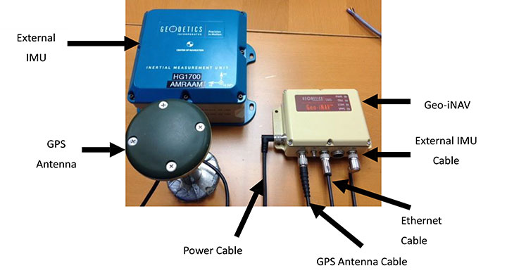
This technology is implemented in a rugged modular platform (Figure 3) with three main units:
A dual-frequency GPS antenna,
An integrated INS coupling GPS receiver with either an internal MEMS IMU or external IMU,
An external fiber-optic gyroscope (FOG) IMU for high-end accuracy and reliability. The external IMU is optional and dedicated to increasing the DR capability.
Figure 3. Dual-frequency differential navigation unit hybridized with external fiber-optic gyro.
Performance. Tests have been performed in conditions close to the land-vehicle navigation validation. It is based on measurements on-the-fly with no post-processing except for evaluation of the error.
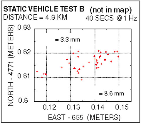
The first case is a static position of the rover 4.8 kilometers away from the reference receiver. Positions are updated once per second. The system includes a FOG IMU. the lateral error peak is less than 4 centimeters. Bias error is less than 1 centimeter. See Figure 4.
Figure 4. Single point error when rover is static.
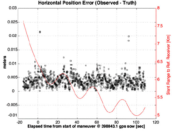
The second test case is with a high-dynamic mobile platform, moving at a speed of 200 km/h, with an average distance from the reference to the rover of 6 kilometers. Lateral error standard deviation is 0.5 centimeters, peak error is less than 2.2 centimeters. Bias error is lower than 0.2 centimeters (Figure 5).
Figure 5. Dynamic trial test single point error.
The performance in these test cases meets the expected accuracy for validation of autonomous navigation.
One last method to increase accuracy is to switch to a different class of IMU performance, from tactical grade to advanced. When in the line-of-sight of the GNSS sky-view, the performance is the nearly the same.
Conclusion
A real-time, differential Epoch-by-Epoch, dual-frequency carrier-phase GPS receiver, tightly hybridized with a high-performance IMU can provide absolute error lower than 5 centimeters in the 10-kilometer baseline range of the reference static receiver. This is fully adapted to the qualification of driverless auto-pilot systems for the targeted year of 2020. It can avoid the need to use complex theodolite and vision calibration systems. It provides maximum flexibility and minimum sustaining costs.
Acknowledgment
This study has been made possible thanks to materials provided by Geodetics Inc. and the advice of Jeffrey A. Fayman, vice president, Business & Product Development, Geodetics Inc. The results displayed in Figures 4 and 5 are from a test with a medium-sized UAV from Allied Drones, model EF44 high-endurance quad.
Manufacturers
The Geo-iNAV family is a range of GPS-aided INS solutions available in different configurations, including various GPS receivers (L1, L1/L2 RTK, SAASM), internal MEMS or external FOG IMU. As part of this family, the Geo-RelNAV provides differential GPS relative navigation capability, the Geo-hNAV includes a dual GPS antenna receiver for static heading measurement capability, and the Geo-PNT combines position and attitude measurement with precise timing distribution.
Gilles Boime is is chief scientist for Spectracom. He is involved in GNSS signal generator, hybridized navigation platforms, GNSS timing and synchronization innovative solutions build-up. He holds an engineering diploma in telecommunication from Institut Superieur d’Electronique de Paris.
Emmanuel Sicsik-Pare is strategic product manager for Spectracom. He is involved in timing and navigation products and systems definition and application market monitoring. He holds a M.Sc degree from Telecom Bretagne.
John Fischer is CTO of Spectracom. He has more than 30 years experience creating navigation and communications systems, received his master’s in electrical engineering from SUNY at Buffalo. Prior to joining Spectracom, he worked in radar, command and control, and wireless systems.