Tag: geoid model

  • The effects of geoid changes in NGS’s new, modernized 2022 NSRS

    The effects of geoid changes in NGS’s new, modernized 2022 NSRS

    My April column addressed the vertical movement at the NOAA CORS Network (NCN). The values at the sites indicate the potential movement of marks in the area of the CORS. The rates are based on GNSS data and have an estimate of error associated with them.

    As I mentioned in my previous column, I’m not sure how the National Geodetic Survey (NGS) will address the vertical movement effects in the new, modernized National Spatial Reference System (NSRS). That said, NGS will be monitoring the CORS and looking for trends to help describe the vertical movement at the CORS. These trends are an indication of what may be happening in that area.

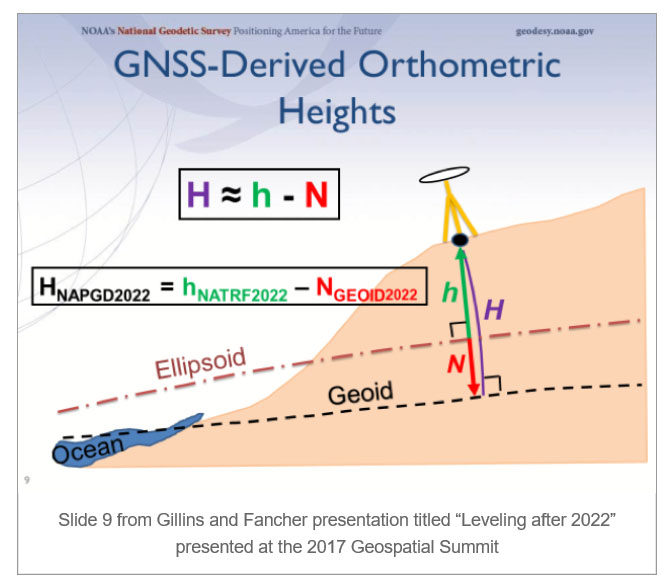
    As stated in previous columns, orthometric heights in NAPGD2022 will be defined through ellipsoid heights and a geoid model, for example GEOID2022. In addition to the movement of individual marks due to crustal movement, there are geophysical reasons for changes in the geoid that affect the orthometric height of a mark. Therefore, changes in the geoid model will be very important to users estimating orthometric heights using GNSS.

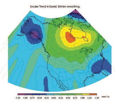
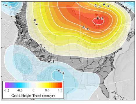
    As stated in the NOS NGS 64 report, NGS has set a goal of maintaining geoid accuracy at 1 centimeter (1 standard deviation) in both absolute and differential geoid undulations. The box titled “Figure 13 from NOS NGS 64 Report” depicts an estimate of the secular change in the geoid. As indicated in the plot, the changes are very small, ranging from -1.25 mm/year to 1.5 mm/year.

    What I find interesting is the small negative change in the southeastern United States. There are other drivers for geoid changes. This column will address some of these changes and what they mean to users.

    Secular geoid change

    Photo: NGS
    Figure 13 from NOS NGS 64 Report (Image: NGS)

    As mentioned in many of my articles, the new, modernized NSRS has a time-dependent component. This includes the geoid modelTable 5-1 from NOS NGS 64 report are examples of some of the physical processes being investigated by NGS to account for changes in the geoid.  (See the box titled “Some of the geophysical drivers of geoid change.”) As mentioned in the NOS NGS 64 report, the magnitudes in red have already been determined to be too small for NGS to model. The examples highlighted in yellow have magnitudes that are significant and NGS will attempt to account for these changes to the geoid. 

    Table 5-1: Some of the geophysical drivers of geoid change
    Table 5-1: Some of the geophysical drivers of geoid change

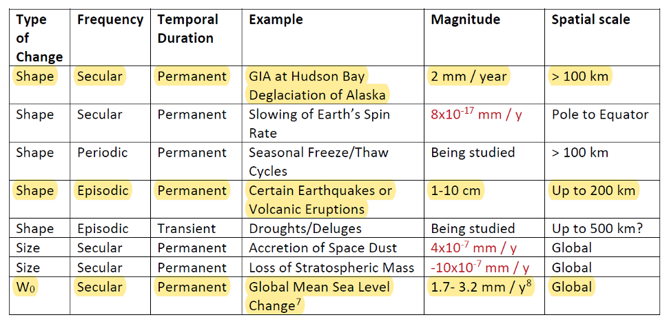
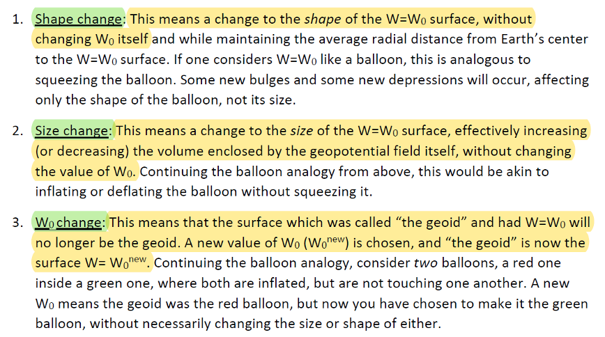
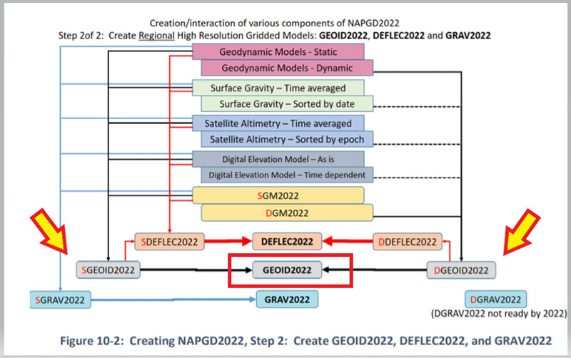
    NGS classifies the changes in the geoid in three different groups: Shape Change, Size Change, and W0 Change. The box titled “The Groups of Geoid Change” provides NGS’s definition and explanation of the terms.

    The groups of geoid change

    Photo: Dave Zilkoski

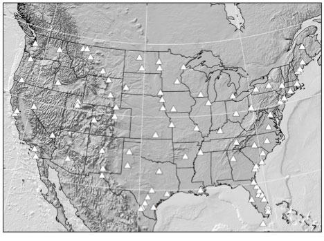
    NGS’s report on their Geoid Monitoring Service (GeMS) program provides figures that depict an estimate of the secular geoid rate trend based on the NASA GSFC mascon model. See the boxes titled “Estimate of Geoid Rate Over CONUS” and “Estimate of Geoid Rate Over Alaska.” For more details on GeMS, download the report NOAA Technical Report NOS NGS 69: A Preliminary Investigation of the NGS’s Geoid Monitoring Service (GeMS), and read my December 2019 Survey Scene column. The secular geoid rate trend is an example of the geoid changing its shape, but not the W0 value. What this means is that the local geoid undulations will change, but the overall size of the geoid will not.

    Estimate of geoid rate over CONUS

    Figure 32: Geoid rate over CONUS based on the GSFC mascon model [mm/yr] (Image: NOAA)
    Figure 32: Geoid rate over CONUS based on the GSFC mascon model [mm/yr] (Image: NOAA)
    Estimate of geoid rate over Alaska

    Figure 33: Geoid rate over Alaska from GSFC mascon model [mm/yr] (Image: NOAA)
    Figure 33: Geoid rate over Alaska from GSFC mascon model [mm/yr] (Image: NOAA)
    These changes in the geoid are fairly small values (+/- 1.3 mm/year), but they will accumulate over a decade. As previously stated, NGS’s goal is to maintain geoid accuracy at the centimeter level (1 standard deviation) in both absolute and differential geoid undulations. In my February 2022 column, I discussed how coordinates change because Earth’s surface is moving due to the movement of major tectonic plates. It’s fairly obvious how the tectonic shift affects horizontal coordinates, but earthquakes and volcanic eruptions can also cause large shifts in vertical coordinates.

    In recent history, on May 18, 1980, geologists watched in awe as Mount St. Helens erupted in a gigantic explosion. After the eruption, the volcanic cone of Mount St. Helens had been completely blasted away; the peak, which was at an elevation of 9,677 feet (2,950meters) was changed to a horseshoe-shaped crater with an elevation of 8,363 feet (2,549 meters). Extreme crustal movements such as the Mount St. Helens eruption can change the shape of the geoid. As explained in my April 2022 newsletter, NGS understands this and is attempting to manage the changing coordinates by providing a time-dependent component to a mark’s ellipsoid height, but there is also a time-dependent component to the geoid that affects the mark’s orthometric height.

    Ring of Fire

    Image: National Ocean Service
    Image: National Ocean Service

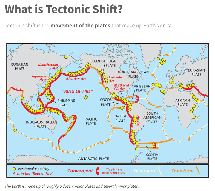
    The “Ring of Fire” map highlights earthquake activities around the world. As indicated in Table 5.1, earthquake or volcanic eruptions can change the shape of the geoid. Of course, they also can change the height of a mark due to crustal movement, which would typically be larger than the change in the geoid height. The amount of movement would be due to the size and magnitude of the event, but even small earthquakes could cause a change in the height of a mark located near the event. Earthquakes are occurring all over the world every day. 

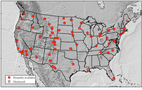
    Earthquakes with large magnitudes are highlighted by news media outlets, but ones with smaller magnitude typically are not highlighted. The four figures below provide examples of earthquakes that have occurred over 30 days. This information can be obtained from the United States Geological Survey (USGS).

    Earthquakes during the past 30 Days
    Date: May 20, 2022

    Image: USGS
    Image: USGS

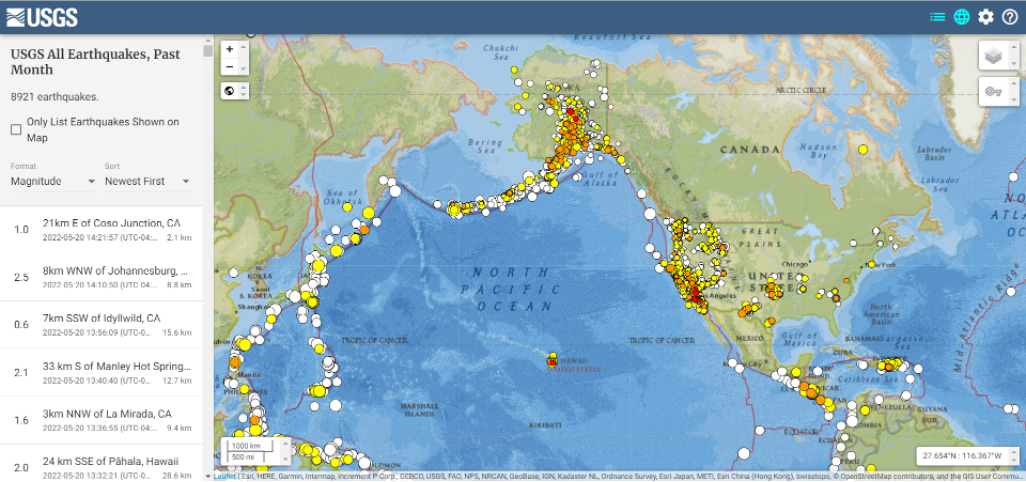
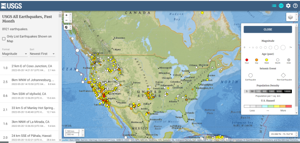
    Earthquakes in the lower 48 during the past 30 days
    Date: May 20, 2022

    Image: USGS
    Image: USGS

    Earthquakes in eastern United States in the past 30 days
    Date: May 20, 2022

    Image: USGS
    Image: USGS

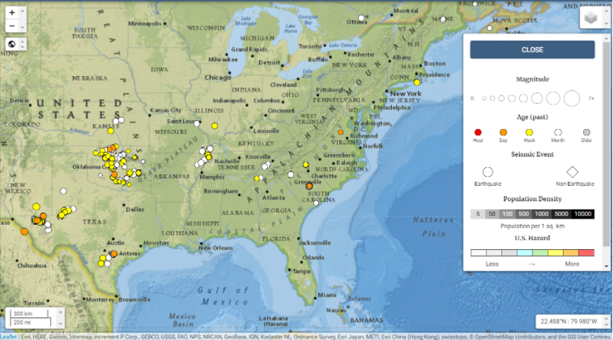
    I found the large number of earthquakes that occurred in Oklahoma in just 30 days to be very interesting.  This isn’t something that I thought occurred in the eastern region of the United States. 

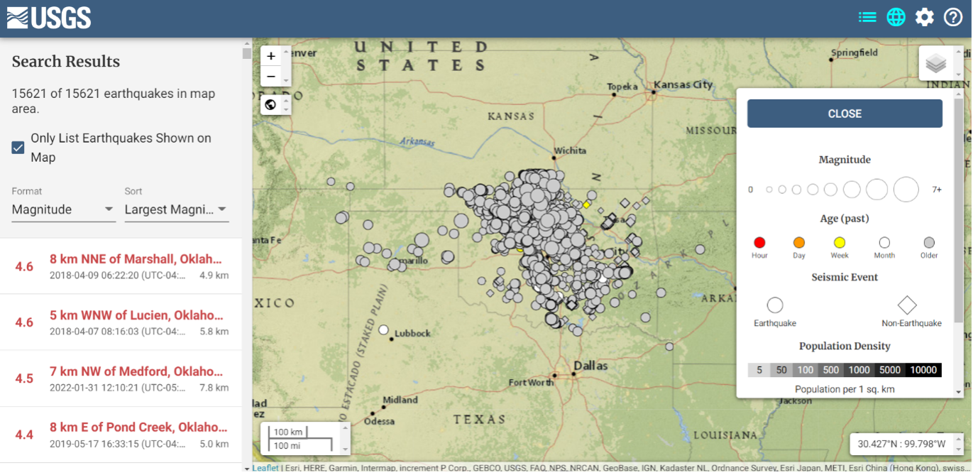
    Earthquakes in Oklahoma during the past 30 days
    Date: May 20, 2022

    Image: USGS
    Image: USGS

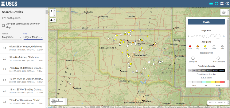
    The image below depicts earthquakes that have occurred in Oklahoma in the past five years. They are fairly small in magnitude, but what is the cumulative effect on the geoid in the region, as well as changes to the orthometric heights of marks due to crustal moment in the region?  This is why it is important for the new, modernized NSRS to implement time-dependent coordinates. 

    Earthquakes in Oklahoma in the last 5 years
    Dates: 2017 to 2022

    Image: USGS
    Image: USGS

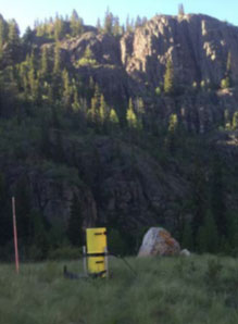
    To better understand the changes to the geoid, NGS performed a survey in Alaska to obtain geodetic data as part of its GeMS program.  On May 12, 2022, Kevin Ahlgren, a geodesist at NGS, described in a webinar the observations collected and some of the results. 

    The presentation provided an overview of a field campaign performed in support of the GeMS program and a time-dependent geoid model. The campaign included static GNSS, relative gravity, and deflection of the vertical techniques on 50 stations in Alaska. The webinar was can be downloaded.

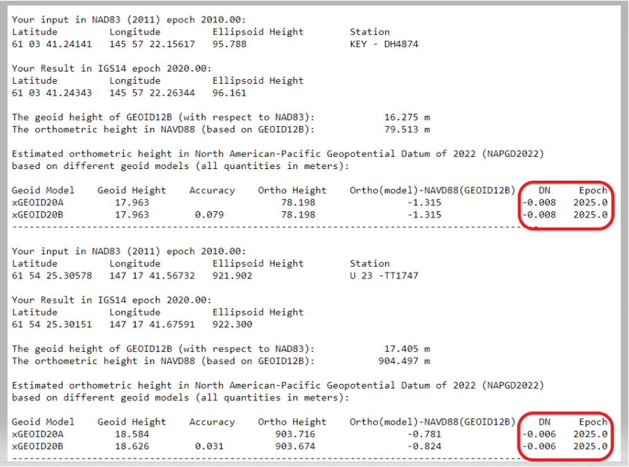
    I encourage everyone to download the presentation.  The change in the geoid due to geophysical drivers is small, but if the new, modernized NSRS is going to include time-dependent coordinates, then changes in the geoid must be accounted for.  For demonstration purposes, NGS provides an example of the time-dependent geoid change in the xGEOID20 webtool.  The box below, “xGEOID20 interactive computation output,” is an example of using this tool. The two stations are located in Alaska. As indicated in the output from the tool, the change in the geoid is 8 mm in five years. Again, NGS’s goal is to maintain geoid accuracy at the centimeter level (1 standard deviation) in both absolute and differential geoid undulations.  These small changes can become significant over time. 

    xGEOID20 interactive computation output

    Note: DN is the time-dependent geoid change computed between user inputted epoch (t) and t.
    Note: DN is the time-dependent geoid change computed between user inputted epoch (t) and t. (Image: NGS)

    The last geoid change group that I’ll highlight has to do with the change in the gravity potential (W0) value that defines the model. The NOS NGS 64 Report states that the standing definition of the geoid, as adopted and used at NGS, is the following:  

    The geoid is the equipotential surface of the Earth’s gravity field which best fits, in a least squares sense, global mean sea level. 

    As stated in the NOS NGS 64 report, over a century of sea-level measurements imply that global mean sea level (GMSL) was rising at a rate of approximately 1.7 millimeters per year and was rising at a rate of 3.2 millimeters per year between 1993 and 2010 (IPCC, 2014). If NGS is going to define the geoid as the equipotential surface of the Earth’s gravity field that best fits, in a least squares sense, global mean sea level, then the geoid in the new, modernized NSRS must change when the GMSL exceeds a certain threshold. 

    Again, NGS’ goal is to maintain geoid accuracy at the centimeter level (1 standard deviation) in both absolute and differential geoid undulations.  What this means is that as GMSL rises, the value of gravity potential which best fits to GMSL (called W0) will also change.  In other words, the surface which was called “the geoid” and had W=W0 in 2022 will no longer be the geoid. A new value of W0 (W0new) is chosen, and “the geoid” would now be the surface W=W0new.   

    So, what does this really mean to users? The NOS NGS 64 Report states on page 37:

    “NGS and the Canadian Geodetic Survey have jointly adopted the value of 2.0 m^2/s^2 as the replacement threshold for a new geoid model (and new geopotential datum). This represents approximately 20 centimeters of GMSL (and thus geoid) rise. At the current rate of sea-level change of about +3 millimeters per year (IPCC, 2014), this means NGS expects to replace NAPGD2022 in approximately 60 to 70 years.” 

    Therefore, this should not be a major concern of users for a long time. 

    This column highlighted that orthometric heights in NAPGD2022 will be defined through ellipsoid heights and a geoid model, for instance GEOID2022; and therefore, changes in the geoid model will be very important to users estimating orthometric heights using GNSS.  It briefly described the geophysical reasons for changes in the geoid that affect the orthometric height of a mark. 

    If NGS is going to meet the goal of maintaining geoid accuracy at 1 centimeter (1 standard deviation) in both absolute and differential geoid undulations, they will have to address changes in the geoid. The secular changes in the geoid, as indicated in Figure 13 in the NOS NGS 64 report, are very small, ranging from -1.25 mm/year to 1.5 mm/year. Once again, these are small changes to the geoid, but they will accumulate over time, and that is why NGS is including time-dependent coordinates in the new, modernized NSRS.

  • How NGS can implement a time-dependent geopotential datum

    How NGS can implement a time-dependent geopotential datum

    The National Geodetic Survey (NGS) has published a technical report that describes options for how NGS can implement a time-dependent geopotential datum and thus a time-dependent geoid model. My last column described the latest version of NGS’ VERTCON model. As mentioned in the column, NGS is developing these models and tools to support the implementation of the North American-Pacific Geopotential Datum of 2022 (NAPGD2022).

    NAPGD2022 is going to be a time-dependent geopotential datum. In other words, the reference geopotential will change over time and therefore the geoid height value will change over time. NAPGD2022 was described in detail in NGS’ publication “Blueprint for 2022, Part 2: Geopotential Coordinates,” and my December 2017 column. Blueprint for 2022, Part 2 states that a gridded geoid model GEOID2022 will be created and it will contain two components:

    1. The first component will be time independent, denoted as the Static Geoid model of 2022 (SGEOID2022).
    2. The second component will be a time-dependent geoid undulation model, encompassing permanent geoid changes greater than or equal to 1 millimeter per year, denoted as Dynamic Geoid model of 2022 (DGEOID2022).

    NGS will publish a GEOID2022 value that will be based on both SGEOID2022 and DGEOID2022. As stated in the document, GEOID2022 will be the official zero-height surface for orthometric heights within NAPGD2022, and thus within the NSRS. The box titled “Excerpt from Blueprint for 2022, Part 2, Figure 10-2” is a diagram that describes the process of creating the regional high resolution gridded GEOID2022 model. I have highlighted the GEOID2022 model and its two components, SGEOID2022 and DGEOID2022.

    Excerpt from Blueprint for 2022, Part 2, Figure 10-2

    Image: National Geodetic Survey
    Image: National Geodetic Survey

    First, it’s important to note the role of the geoid in estimating GNSS-derived orthometric heights. As described in a previous column, GNSS-derived Orthometric Heights are computed using the following formula: orthometric height (H) = ellipsoid height (h) minus geoid height (N). See the box titled “NAPGD2022 GNSS-Derived Orthometric Height.”

    NAPGD2022 GNSS-Derived Orthometric Height

    Source: Slide 9 from Gillins and Fancher presentation titled ‘Leveling after 2022’ presented at the 2017 Geospatial Summit
    Source: Slide 9 from Gillins and Fancher presentation titled “Leveling after 2022” presented at the 2017 Geospatial Summit

    So, what does it take to compute a time-dependent geoid model and what is NGS’ plan to accomplish this project The technical report titled “ A Preliminary Investigation of the NGS’s Geoid Monitoring Service (GeMS)” describes options for how NGS can implement a time-dependent geopotential datum and thus a time-dependent geoid model (See box titled “NGS Publishes Report on GeMS”). The report contains too much information for a single column. This column will highlight some of the sections of the report. The document does contain a lot of technical information and I would encourage everyone to download the document.

    NGS Publishes Report on GeMS

    Screenshot: National Geodetic Survey
    Screenshot: National Geodetic Survey

    The technical report describes the current state of knowledge and outlines next steps required to define a time-dependent geopotential datum for the Nation. NGS created a project called “The Geoid Monitoring Service,” or simply GeMS, to accomplish their long-term goal of establishing a time-dependent geopotential model.

    The report addressed the following five topics:

    1. A foundational introduction to the various types of geophysical phenomena that are causing both size and shape change to the geoid,
    2. Geodetic observing techniques that are presently available to monitor geoid change,
    3. An objective evaluation of NGS’s current ability to incorporate these techniques into a long-term monitoring service like GeMS,
    4. Known barriers to accomplishing such a project, and
    5. Potential observing techniques that might become available in the next 10-20 years, but are not currently mature enough for operational use.

    The document presents a roadmap of options for how NGS could realize a time-dependent geopotential datum, and how NGS can support the dynamic datum into the future with independent validation surveys and datasets.

    The report discusses the available geoid monitoring techniques that NGS has to support modeling the changes in the geoid. There are three existing NGS program areas and associated technical expertise that could be utilized in an operational GeMS:

    1. NGS’s Gravity Program,
    2. the NOAA CORS Network, and
    3. GPS/geodetic leveling campaigns.

    It is noted that individuals these techniques cannot provide 100% of what GeMS requires but combining various programs would be sufficient. The report does a great job of describing these three program areas. The box titled “Summary of Geoid Monitoring Techniques within NGS’ Current Expertise” is Table 3 from the Technical Report. The table list the affordability and accuracy attributes for each of the program areas. NGS’ Gravity Program provides high quality gravity data to internal and external stakeholders. The program provides gravity data required for NGS’s geoid modeling.

    Summary of Geoid Monitoring Techniques within NGS’ Current Expertise

    Source: National Geodetic Survey
    Source: National Geodetic Survey

    The report provides a good overview of the expertise and instrumentation of NGS’ Gravity Program. The table titled “Summary of NGS’ Terrestrial Gravity Instruments” is a compilation of information on historical methods and instrumentation from the technical report.

    Summary of NGS’ Terrestrial Gravity Instruments

    The document highlights something about the United States gravity data that most users don’t think about. That is, gravity values are referenced to a gravity network just like NGS’ published orthometric heights are referenced to the NAVD 88. In the mid-1950s, a coordinated effort was initiated by the International Association of Geodesy (IAG) to make gravimeter ties throughout collaborating parts of the world to support establishment of an International gravity datum.

    It incorporated intercontinental, north-south, calibration lines and long-distance ties established by airplane. The majority of USA relative gravimeter work was done from 1965 – 1967, resulting in the network shown in the box titled “International Gravity Station Net of 1971 (IGSN71) in CONUS.” The report states that the calculations were completed by Urho A. Uotila of The Ohio State University around 1970.

    The gravity network was constrained by a network of ballistic absolute gravimeters. Five of the eight absolute gravimeter sites were in CONUS. It was a world-wide, simultaneous adjustment and published as The International Gravity Standardization Net 1971 (I.G.S.N. 71). A

    s of December 2019, the IGSN71 remains the official international gravity datum. Many of these stations have been destroyed over the decades, in particular those at passenger airport terminals.

    International Gravity Station Net of 1971 (IGSN71) in CONUS

    (Source: Figure 14 from geodesy.noaa.gov)

    Figure 14: IGSN71 Gravity Stations. (Source: National Geodetic Survey)
    Figure 14: IGSN71 Gravity Stations. (Source: National Geodetic Survey)

    In the mid-1970s, NGS was involved in two major readjustment projects, replacement of NAD27 with NAD 83 and the replacement of NGVD 29 with NAVD 88. At the same time, the NGS gravity group were evaluating the gravity data in NGS database and the gravity stations involved in the IGSN71. During the period 1975 and 1979, NGS and NGA (formally DMA) performed relative gravity surveys around CONUS to evaluate the stations.

    A report by Robert Moose titled “The National Geodetic Survey Gravity Network” published by NGS in 1986 documents the results of the surveys. This network is denoted as the National Geodetic Survey Gravity Network (NGSGN) and depicted in the box titled “National Geodetic Survey Gravity Network (NGSGN) in CONUS.” The NGSGN was constrained by 8 absolute gravimeter stations and consisted of 232 stations. Differences between NGSGN values and IGSN71 values were computed to evaluate or detect change in gravity values.

    The box titled “Gravity Differences between NGSGN and IGSN71 Common Stations” depict these differences. The report states “In summary, the gravity differences between NGSGN and IGSN are generally small and many of the larger differences may be due to vertical motion.

    National Geodetic Survey Gravity Network (NGSGN) in CONUS

    (Source: Figure 15 from geodesy.noaa.gov)

    Figure 15: NGSGN Stations. Destroyed stations known as of July 2019. (Source: National Geodetic Survey)
    Figure 15: NGSGN Stations. Destroyed stations known as of July 2019. (Source: National Geodetic Survey)

    Gravity Differences between NGSGN and IGSN71 Common Stations

    (Source: Figure 16 from geodesy.noaa.gov)

    Figure 16: Difference between NGSGN and IGSN71 AG values [mgal] (Source: National Geodetic Survey)
    Figure 16: Difference between NGSGN and IGSN71 AG values [mgal] (Source: National Geodetic Survey)
    The basic rule of thumb for estimating land movement using gravity changes is: 1 meter of change equals 0.3086 mgals (1 cm of change equals 0.003086 mgals). It should be noted that a positive difference in gravity in the figure indicated apparent subsidence. As stated by the 1986 report by Moose, the large difference in Houston-Galveston region is most likely due to subsidence.

    A report documenting the apparent movement in the Houston-Galveston region was published by NGS in 1980. The boxes titled “ Estimate of Subsidence in Houston-Galveston Area During 1963-78 Epoch” and “Estimate of Subsidence in Houston-Galveston Area During 1973-78 Epoch” provide estimates of the movement in the region that include the same epoch of the two gravity networks. These two plots agree with the summary statement in the 1986 report.

    Estimate of Subsidence in Houston-Galveston Area During 1963-78 Epoch

    (Source: Figure 7 from ngs.noaa.gov)

    NOTE: 30 cm approximately equals to 1 foot (Source: National Geodetic Survey)
    NOTE: 30 cm approximately equals to 1 foot (Source: National Geodetic Survey)

    Estimate of Subsidence in Houston-Galveston Area During 1973-78 Epoch

    (Source: Figure 8 from https://www.ngs.noaa.gov/PUBS_LIB/The1978Houston_Galveston_and_Texas_GulfCoast_VerticalControlSurveys_TM_NOS_NGS27.pdf)

    NOTE: 30 cm approximately equals to 1 foot (Source: National Geodetic Survey)
    NOTE: 30 cm approximately equals to 1 foot (Source: National Geodetic Survey)

    What does all this mean to the geoid? Accurate and current gravity data are critical to the development of an accurate geoid model that includes estimating changes in the geoid model over time.

    The technical report on NGS’ Geoid Monitoring Service (GeMS) describes geodetic and geophysical techniques that are currently known to NGS and show promise for GeMS (see the box titled “Summary of Known Geoid Monitoring Techniques that are currently outside of NGS’s Expertise). It should be noted that all of these techniques rely on a non-NGS entity to create a product (such as a model or dataset) that NGS can utilize in their products and services. This is nothing new; NGS leverages partnerships for other products such as the GOCO05S satellite gravity model produced by an ESA consortium led by the Technical University of Munich. This model is used by the NGS geoid team in static geoid modeling.

    Summary of Known Geoid Monitoring Techniques that are currently outside of NGS’s Expertise

    (Source: Table 7 from Technical Report NOS NGS 69)
    (Source: Table 7 from Technical Report NOS NGS 69)

    Continuation of Summary of Known Geoid Monitoring Techniques that are currently outside of NGS’s Expertise

    (Source: Table 7 from Technical Report NOS NGS 69)
    (Source: Table 7 from Technical Report NOS NGS 69)

    As apparent by all of the types of data required to monitor the geoid, NGS has a challenging task to establish a Geoid Monitoring Service. Why is it important to invest resources to monitor the geoid? Analyzes of temporal satellite gravity missions provide changes in gravity values that can be use to create changes in the geoid. The GRACE (Gravity and Climate Experiment) satellite mission was designed to provide the temporal gravity field variations throughout its mission (duration 2002 – 2017). There are analysis centers that produce models using the GRACE data – University of Texas at Austin Center for Space Research (UTCSR), NASA Jet Propulsion Laboratory (JPLEM), and GFZ German Research Center for Geosciences (GFZOP). Release 6 denoted as RL06 is the most current GRACE data from these groups.

    The data can be used to illustrate the magnitudes and resolutions that GRACE models provide to the seculargeoid rates for CONUS and Alaska. The boxes titled “GRACE Trend over CONUS from UTCSR RL06” and “GRACE Trend over Alaska from UTCSR RL06” are plots from Technical Report NOS NGS 69 that show these secular geoid trends from UTCSR-RL06. The plots indicate very small changes in the geoid but they are significant if the goal is to monitor the geoid model to the mm/year level.

    GRACE Trend over CONUS from UTCSR RL06

    Figure 27: GRACE Trend over CONUS from UTCSR RL06 Model [mm/yr] (Source: Figure 27 from Technical Report NOS NGS 69)
    Figure 27: GRACE Trend over CONUS from UTCSR RL06 Model [mm/yr] (Source: Figure 27 from Technical Report NOS NGS 69)

    GRACE Trend over Alaska from UTCSR RL06

    Figure 28: GRACE Trend over Alaska from UTCSR RL06 GRACE Model [mm/yr] (Source: Figure 28 from Technical Report NOS NGS 69)
    Figure 28: GRACE Trend over Alaska from UTCSR RL06 GRACE Model [mm/yr] (Source: Figure 28 from Technical Report NOS NGS 69)
    Another product available from various processing centers are surface mass concentrations (mascons) as observed by the GRACE satellites. Once again, these mascons can be used to generate a secular geoid rate. The boxes titled “Geoid rate over CONUS based on the GSFC mascon model” and “Geoid rate over Alaska from GSFC mascon model” are plots from Technical Report NOS NGS 69 that provide the secular geoid rate based on the NASA GSFC mascon model. Once again, the plots indicate very small changes in the geoid but there is a systematic change to the geoid based on the analysis of the data from the GRACE mission.

    Geoid rate over CONUS based on the GSFC mascon model

    Figure 32 From Technical Report NOS NGS 69: Geoid rate over CONUS based on the GSFC mascon model [mm/yr] (Source: Figure 32 From Technical Report NOS NGS 69)
    Figure 32 From Technical Report NOS NGS 69: Geoid rate over CONUS based on the GSFC mascon model [mm/yr] (Source: Figure 32 From Technical Report NOS NGS 69)

    Geoid rate over Alaska from GSFC mascon model

    Figure 33 From Technical Report NOS NGS 69: Geoid rate over Alaska from GSFC mascon model [mm/yr] (Source: Figure 33 From Technical Report NOS NGS 69)
    Figure 33 From Technical Report NOS NGS 69: Geoid rate over Alaska from GSFC mascon model [mm/yr] (Source: Figure 33 From Technical Report NOS NGS 69)
    The report stated that when considering monitoring the geoid, the greatest change to the geoid from glacial isostatic adjustment (GIA) processes is centered in northern Canada, but there is “still a significant geoid height trend in the Northern Plains, Great Lakes, and Northeast regions of CONUS.”

    It was noted that if GIA processes are not considered, a 1 cm error in the geoid undulation would occur within 18 years. NADGPD2022 orthometric heights are going to be established using a NATRF2022 ellipsoid height and a GEOID2022 geoid height. This is why the geoid needs a time-dependent component.

    This column highlighted NGS new Geoid Monitoring Service (GeMS); and, that NGS’ will be publishing a gridded geoid model GEOID2022 that will contain two components:

    1. The first component will be time independent, denoted as the Static Geoid model of 2022 (SGEOID2022) and
    2. The second component will be a time-dependent geoid undulation model, denoted as Dynamic Geoid model of 2022 (DGEOID2022).

    NGS will publish a GEOID2022 value that will be based on both SGEOID2022 and DGEOID2022. The column provided examples of how GRACE data can be used to illustrate the magnitudes of secular geoid rates for CONUS and Alaska.

  • Eos adds GEOID height support for Arrow GNSS receivers

    Eos adds GEOID height support for Arrow GNSS receivers

    Orthometric height support (survey-grade elevations) enables Arrow GNSS receivers to collect high-accuracy, survey-grade vertical data with any data-collection software.

    Eos Positioning Systems Inc. has added support for GEOID height models within its Arrow Series GNSS receivers. Eos manufactures high-accuracy GNSS receivers for any app running on iOS/Android/Windows devices and using the Eos Arrow Series.

    “You can use Arrow Series receivers with any data-collection software in the world, and benefit from accurate orthometric heights,” Eos CTO Jean-Yves Lauture said. “Our Arrow receivers will output accurate GNSS elevations no matter which data-collection software you use to capture it.”

    Image: Eos Positioning
    Image: Eos Positioning

    With support for GEOID models, Arrow receivers automatically output survey-grade elevations to all iOS and Android data collection software. Support will also soon be available for Windows devices.

    The Arrow receivers now support the entire United States to provide survey-grade elevation in NAVD88 orthometric heights through the GEOID12B (US) model. The Arrow receivers also support the Canadian CGG2013a and HTv2.0 GEOID models for the CGVD2013 and CGVD28 vertical datums, respectively. Additional GEOID models for other countries are planned.

    “Eos is intensely focused on supporting high-accuracy GIS, engineering, surveying and construction users by supporting the latest GEOID elevation models within our GNSS monitoring software,” Lauture said. “Our roadmap remains focused on high-accuracy BYOD users by supporting all iOS, Android and Windows users with this capability.”

    The problem is that typical Bluetooth GNSS receivers usually provide inaccurate, built-in elevation models. This inaccuracy is reflected in the Mean Sea Level  elevation output by those receivers. By outputting orthometric height, the Arrow now solves this problem and turns any smartphone or tablet into a 3D, survey-grade accurate data collection device, the company said.

    Eos has designed this new feature so that users will easily be able to update to new GEOID models as they become available.

    Field technicians in pipeline, construction, engineering, architecture, water and any other industry are finally able to enjoy GNSS location with survey-grade vertical accuracy on their iOS and Android devices, with the data-collection app of their choice and their Eos Arrow receivers.