My February 2020 column provided an analysis of the differences between the latest published hybrid Geoid18 values provided on NGS’ Datasheet and the computed geoid height value using the published NAD 83 (2011) ellipsoid height and NAVD 88 orthometric height. The column highlighted issues on differences due to published heights that have changed since the database pull for Geoid18. It mentioned that future columns will address differences in other portions of CONUS. This column will focus on differences between published Geoid18 values and Geoid12B values in Southern Louisiana. Why are users seeing large differences between the two models?
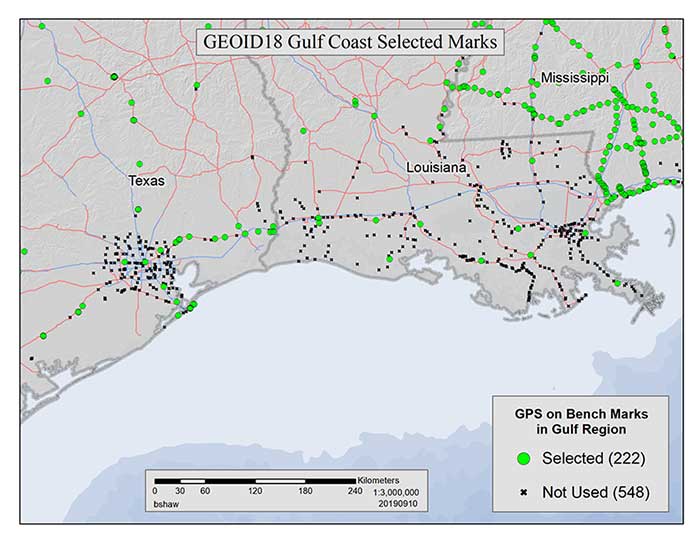
My last column mentioned that the technical report on Geoid18 provided a good explanation on the stations used in the United States Gulf Coast region. See box titled “GPS on Bench Marks for GEOID18 in the Gulf Coast Region.”
GPS on Bench Marks for GEOID18 in the Gulf Coast Region
Figure 1: GEOID18 Gulf Coast selected marks: There are areas of complex vertical crustal motion in the Texas/Louisiana Gulf Coast region of the United States which render many control station elevations in the region invalid. The selection of GPS on Bench Marks in this region was limited to the small number of marks where the leveling and GPS data agreed to minimize the influence of crustal motion in the hybrid geoid model. Figure 1 depicts the selection of stations used in the hybrid geoid model along the Texas/Louisiana Gulf Coast. (Image: National Geodetic Survey)
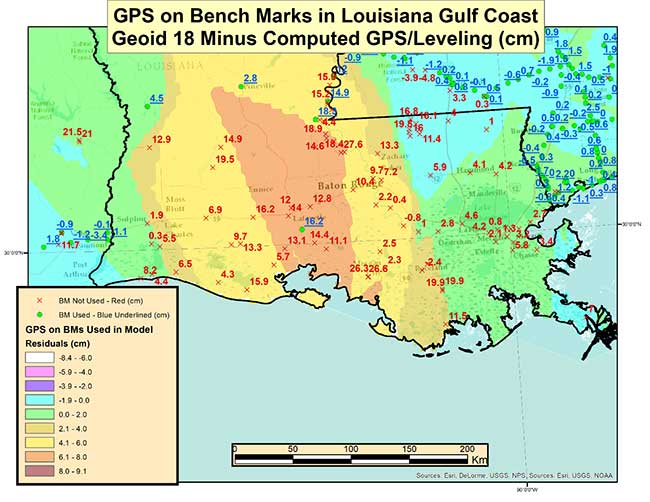
As highlighted in the last column, very few stations in Southern Louisiana were used in the creation of the Geoid18 hybrid geoid model. As provided in my last column the box titled “Differences on GPS on Bench Marks in the Gulf Coast Region” depicts the differences between the published Geoid18 value and the computed geoid value using the latest NAD 83 (2011) ellipsoid and NAVD 88 orthometric height.
Differences on GPS on Bench Marks in the Gulf Coast Region
Image: National Geodetic Survey
The plot indicates that there are many large differences. Many of these differences are to be expected because the Southern Louisiana is an area of known crustal movement. NGS recognizes this and includes the statement below on datasheets for stations published in Southern Louisiana (see box titled “Statement on NGS Datasheet for Stations in Southern Louisiana”).
Statement on NGS Datasheet for Stations in Southern Louisiana
This station is in an area of known vertical motion. Due to the variability of land subsidence, uplift, and crustal motion, NGS has, determined the orthometric heights for marks in these suspect subsidence areas should be considered valid only at the epoch date associated with the orthometric height. These heights must always be validated when used as control. All previously superseded orthometric heights are now considered suspect and are available in the superseded section. NGS does not recommend using suspect or superseded heights as control.
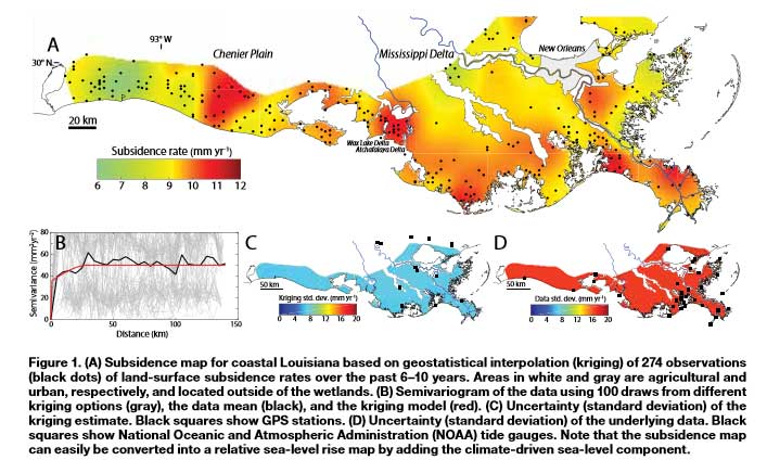
Looking at the figure indicates that there is a significant variation of subsidence occurring in coastal Louisiana. The legend indicates that the subsidence rates range between 0.6 to 1.2 cm/year.
Figure 1 from A New Subsidence Map for Coastal Louisiana
The box titled “Excerpt from Anthropogenic and Geologic Influences on Subsidence in the Vicinity of New Orleans, Louisiana” depicts estimates of crustal movement between 2009 and 2012 in the vicinity of New Orleans. Several of the areas in the plot indicate subsidence rates exceeding -1 cm/year. Once again, the figure shows the local variability of subsidence rates.
Excerpt from Anthropogenic and Geologic Influences on Subsidence in the Vicinity of New Orleans, Louisiana
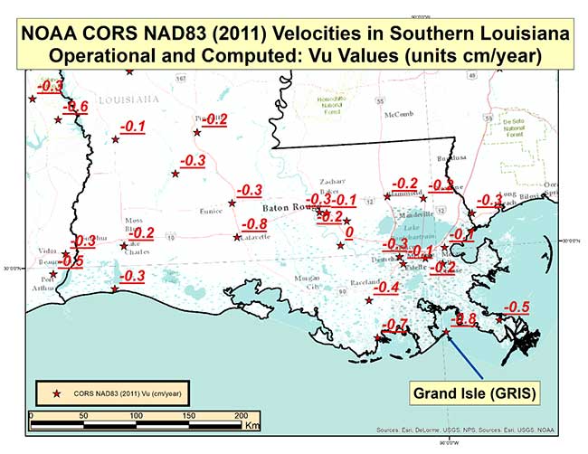
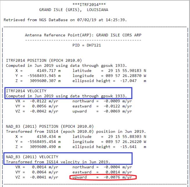
Last year, NGS performed the Multi-Year CORS Solution 2 (MYCS2). This was described in previous columns, which can be viewed here and here. The MYCS2 process generated computed and modeled velocities for CORSs. The box titled “CORS NAD83 (2011) Vu Velocities” is a plot that depicts the velocities in the “upward” component in cm/year for NOAA CORS that are operational and have a computed velocity in Southern Louisiana. So, what does this mean to estimating a hybrid geoid model in Southern Louisiana?
CORS NAD83 (2011) Vu Velocities
Image: National Geodetic Survey
The plot indicates that the rates vary from -0.1 cm to -0.8 cm. It should be noted that these stations are CORS and they are typically installed on structures that may not capture the entire amount of subsidence at the land surface. The box titled “CORS Position and Velocity for Station GRIS” provides an example of a CORS sheet from NGS CORS website.
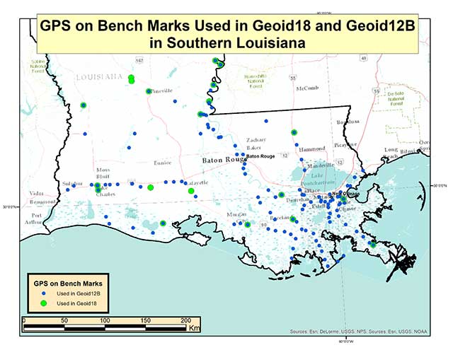
Now, let’s look at differences between Geoid12B and Geoid18 in Southern Louisiana. The box titled “GPS on Bench Marks Used in Geoid18 and Geoid12B” depicts the stations used in Geoid12 and those used in Geoid 18. As indicated in the plots, there were a lot more stations used in the generation of the Geoid12B model than those used to create the Geoid18 model.
GPS on Bench Marks Used in Geoid18 and Geoid12B
Photo: National Geodetic Survey
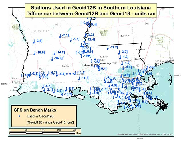
The box titled “Differences between Geoid12B and Geoid18 in Southern Louisiana” provides the values of Geoid12B minus Geoid18 in centimeters on the GPS in Bench Mark stations used in Geoid12B.
Differences between Geoid12B and Geoid18 in Southern Louisiana
Photo: National Geodetic Survey
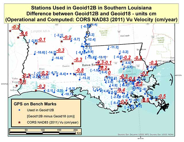
As indicated in the plot, there are some large differences between Geoid12B and Geoid18 values; a few differences exceed 15 centimeters. Based on the previous discussion of crustal movement in Southern Louisiana, this probably shouldn’t come as a surprise. The box titled “Differences between Geoid12B and Geoid18 with Vu Velocity Values” depicts the differences in the hybrid geoid models and the NAD83 (2011) CORS Vu rate.
Differences between Geoid12B and Geoid18 with Vu Velocity Values
Photo: National Geodetic Survey
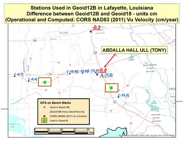
The box titled “Differences between Geoid12B and Geoid18 in Lafayette, Louisiana” depicts the differences in the two hybrid geoid models and the NAD83 (2011) CORS Vu rate values in the Lafayette, Louisiana, region. This region has some of the largest differences between Geoid12B and Geoid18 values in Southern Louisiana. As indicated in the plot, CORS station TONY has a Vu rate of -0.8 cm/year which is fairly large, and the differences between Geoid12B and Geoid18 values are fairly large at the -10 to -15 cm level. Once again, users should expect differences between the two hybrid geoid models because there has been movement in the area and because different GPS on Bench Mark stations were used in the generation of the hybrid geoid models. In the Lafayette region the two stations used in the generation of Geoid18 were not used in Geoid12B (see stations highlighted in a box).
Differences between Geoid12B and Geoid18 in Lafayette, Louisiana
Photo: National Geodetic Survey
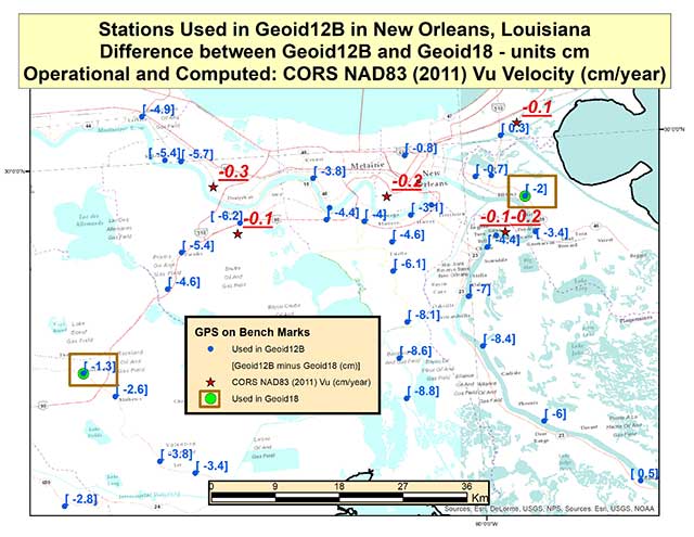
The box titled “Differences between Geoid12B and Geoid18 in New Orleans, Louisiana” depicts the differences in the hybrid geoid models and the NAD83 (2011) CORS Vu rate values in the New Orleans, Louisiana, region. Two of the same stations that were used in the development of Geoid12B and Geoid18 are highlighted with a box. The difference between the two geoid model values are much less in this region compared with the Lafayette region. The CORS Vu velocities are also less than the CORS station (TONY) value in Lafayette. Saying that, the differences on stations not used in Geoid18 have differences ranging from -4 to -8 cm going southward toward the Gulf of Mexico. Once again, Southern Louisiana is subsiding so these differences are not surprising.
Differences between Geoid12B and Geoid18 in New Orleans, Louisiana
Photo: National Geodetic Survey
This means if someone uses NGS’ OPUS web tool to compute a GNSS-derived orthometric height, the NAVD 88 GNSS-derived orthometric height could be significantly different than the published stations in this region. Some of the difference could be due to the difference between the Geoid12B and Geoid18 published values, and some could be due to crustal movement in Southern Louisiana. Saying that, I mentioned in my last column that NGS performed a large GNSS network project in Southern Louisiana in 2016. The GNSS-derived ellipsoid heights were loaded in NGS’ database in March 2019, but the GNSS-derived orthometric height from the 2016 project are not yet finalized so they have not been loaded into NGS’ database. Once finalized and loaded into the database, the 2016 GNSS-derived orthometric heights should be more consistent with GNSS-derived orthometric heights estimated using the NGS’ OPUS web tool. This column focused on differences between published Geoid18 values and Geoid12B values in Southern Louisiana. It provided reasons why users may see large differences between the two models.
This column discusses the results of the National Geodetic Survey (NGS) beta hybrid Geoid18 model and the differences between the beta model and the official hybrid geoid model, Geoid12B. It provides examples to explain the symbology of the Beta Geoid18 Web Map. GEOID18 will be the last hybrid geoid model that NGS will create before NAVD 88 is replaced by the North American-Pacific Geopotential Datum of 2022 (NAPGD2022). I encourage users to access, investigate and become familiar with the web map.
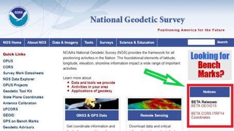
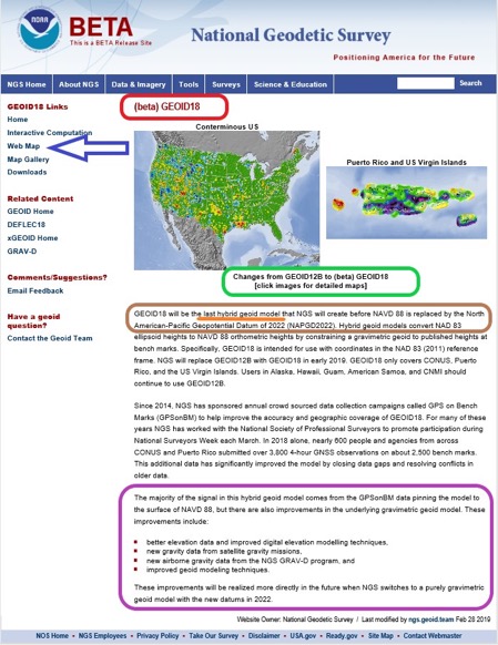
My last column included links to the NGS website that provides the beta coordinates and information about the latest Multi-Year CORS solution (MYCS 2). The column also noted that in late February 2019, NGS released a beta version of the latest hybrid geoid model. See Figure 1, “National Geodetic Survey’s Home Web Page.” This column discusses the Beta Geoid18 Web Map, the results of the hybrid Geoid18 model, and the differences between the beta model and the official hybrid model, Geoid12B.
Figure 1. National Geodetic Survey’s Home Web Page. (Screenshot: National Geodetic Survey)
The Geoid18 hybrid geoid model can be accessed here. See Figure 2, Excerpt from Beta Geoid18 Website. The site provides an opportunity for users to compute a Beta Geoid18 value for a particular station. I would encourage all users to obtain an understanding of the new hybrid model. Once again, it should be noted that this model is a beta model for users to test their workflows and should never be used for official or production work. This allows users to identifies potential issues and differences between Geoid12B and Geoid18, and then contact NGS if they have a question. NGS has done a tremendous job of explaining the Geoid18 process and results, and would appreciate users helping to evaluate the new hybrid model. Several of my previous columns have highlighted the NGS GPS on Bench Marks (GPS on BMs) program and how users have supported the development of the hybrid Geoid18 model: Part 5, Part 6, Part 7, Part 8 and Part 9.
The NGS Beta Geoid18 website provides access to GIS tools that allow users to identify changes between Geoid12B and Geoid18 in their area of interest. The site also states that the hybrid geoid model, Geoid18, will be the last hybrid geoid model that will be created before the new geopotential datum, NAPGD2022, is adopted as the official datum. This is the opportunity for users to be involved in the analysis of the Beta hybrid geoid model. NGS will consider changes to the Beta model until it becomes an official published product. This hybrid geoid model is slightly different from the previous hybrid geoid model, Geoid12B. Similar to Geoid12B, the majority of the design of the hybrid model comes from the relationship between the NGS’ GNSS-derived ellipsoid-derived heights and the leveling- derived orthometric NAVD 88 heights. In other words, the hybrid model is designed to fit to the NAVD 88 orthometric heights.
That said, since the creation of hybrid Geoid12b, there have been improvements in the underlying gravimetric geoid model used in Geoid18. These improvements include:
Better elevation data and improved digital elevation modelling techniques,
New gravity data from satellite gravity missions,
New airborne gravity data from the NGS GRAV-D program, and
Improved geoid modeling techniques.
My previous columns have focused on procedures and routines for establishing GNSS-derived orthometric heights. As I’ve mentioned in these columns, there are many ways to analyze and investigate GNSS data and adjustment results. I have provided basic concepts that I believe are important for users to understand. My October 2016 column focused on the NGS “GPS on BMS (GPSBM)” dataset that was used to create the last hybrid geoid model, Geoid12B.
As mentioned in my October 2015 column, the hybrid geoid model is designed to fit the published NAVD 88 leveling-derived orthometric heights. I highlighted that the GPS on BMs dataset can be used to identify potential issues in the NAVD 88 published orthometric heights. The October 2016 column provided tools and routines that can be used to identify potential issues in NAVD 88 heights and/or NAD83 (2011) published ellipsoid heights. In support of the Beta Geoid18, NGS performed a detailed analysis of the GPS on BMs stations that were used in the creation of Geoid18.
Figure 2. Excerpt from Beta Geoid18 Website. (Image: National Geodetic Survey)
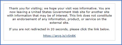
If you click on the “Web Map button” on the Geoid18 web page (see arrow in Figure 2), you may see the statement highlighted in Figure 3. Clicking on the link will redirect you to the correct web site (see Figure 4.).
Figure 3. Result of Clicking on Web Map Button (Screenshot: National Geodetic Survey)
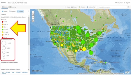
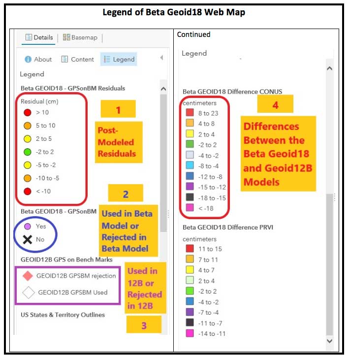
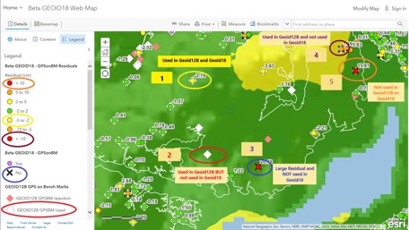
Figure 4. Web Map Option – Results after clicking https://arcg.is/vSn8K (Top Level of Beta Geoid18 Map) [Screenshot: National Geographic, Esri, Garmin, HERE, UNEP-WCMC, USGS, NASA, ESA, METI, NRCAN, GEBCO, NOAA, increment P Corp. | National Oceanic and Atmospheric Administration (NOAA), National Ocean Service (NOS), National Geodetic Survey (NGS)]This data layer provides the value of the post-modeled residuals for all of the GPS on Bench Marks that were part of the evaluation of the Beta GEOID18 model. This Feature Layer is used to populate several layers in the Beta GEOID18 Web Map including the layers called Residuals and GPSonBM. The data for this web map can be found here.The top level of the Beta Geoid18 Map depicts a high-level picture of the residuals. The residuals are in centimeters and represented by different colors. The larger green and yellow circles represent the number of features in the region. The individual GPS on BMs station information appear as the user zooms down. There is a lot of information provided on the Web Map site. The legend changes to provide more detailed information as the user zooms down on the map. I have highlighted four sections on the legend in Figure 5 and provided an explanation of the layers below:
This data layer provides the value of the post-modeled residuals for all of the GPS on Bench Marks that were part of the evaluation of the Beta GEOID18 model. This Feature Layer is used to populate several layers in the Beta GEOID18 Web Map including the layers called Residuals and GPSonBM. The data for this web map can be found here.
This data layer denotes whether the GPS on Bench Mark was used or rejected in the development of the Beta hybrid geoid GEOID18. The data for this web map can be found here.
This data layer denotes whether the GPS on Bench Mark was used or rejected in the development of the hybrid geoid GEOID12B. This has all of the same attributes as the spreadsheet provided on the NGS GEOID12B web page. More information can be found here.
This is a tile package that displays the difference between GEOID18 and GEOID12B in CONUS. It contains two overlayed raster files, one of which is the estimated error and the other is its hill shade. The data for this web map can be found here.
Figure 5. Legend of Beta Geoid18 Web Map (Screenshot: National Geodetic Survey)
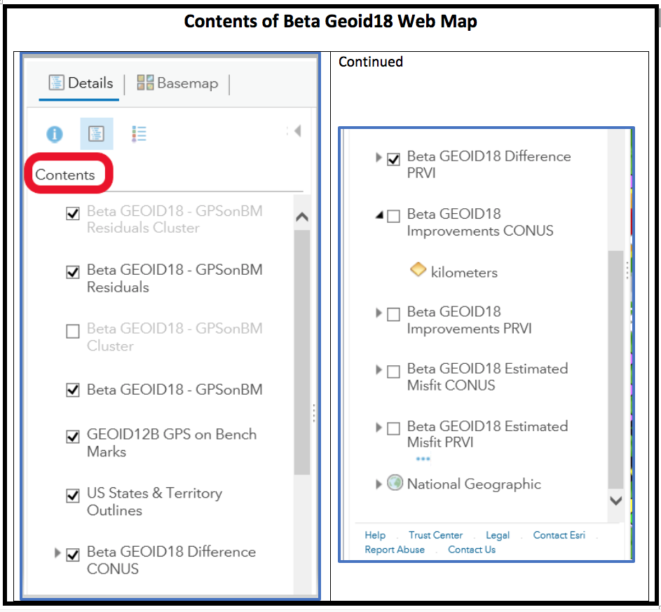
Clicking on the “Content” link provides the data layers (see Figure 6). The user can turn these layers on and off depending on what they’re interested in analyzing.
Figure 6. Contents of Beta Geoid18 Web Map (Screenshot: National Geodetic Survey)
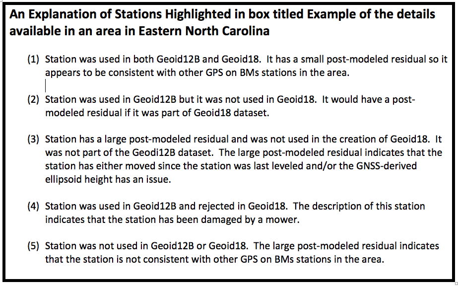
As previously stated, additional details are available as the user zooms into an area of interest (see Figure 7). Five stations have been highlighted in this figure to explain the symbology used on the Web Map site. See Figure 8 for these explanations.
Figure 7. Example of the details available in an area in Eastern North Carolina (Screenshot: National Geodetic Survey)
Figure 8. An Explanation of Stations Highlighted in box titled Example of the details available in an area in Eastern North Carolina (Screenshot: National Geodetic Survey)
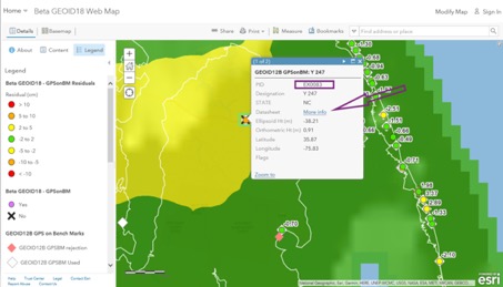
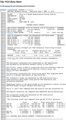
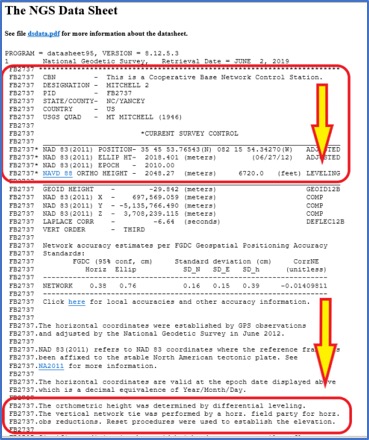
When the user clicks on a station’s icon, another window appears that provides specific information about that station. See Figure 9. If the user clicks on the “More Info” button, the routine retrieves the NGS datasheet from the NGSIDB (see Figure 10). As the NGS datasheet states at the end of the description for station Y 247, the station has been obliterated by a mower, which is why it probably was not used in Geoid18.
Figure 9. Example of Information Available for Individual Stations (Screenshot: National Geodetic Survey)
Figure 10. NGS Datasheet for Station Y 247 (PID EX0083) (Screenshot: National Geodetic Survey)
Figure 11 provides all the information available for station Y 247. It should be noted that the station was used in Geoid12B and not used in Geoid18. This means that there will be differences between Geoid12B and Geoid18 in areas where a station was used in Geoid12B but not used in Geoid18. The amount of the difference will depend on the size of the post-modeled residual. In this example, the post-model residual is 7.39 cm.
Figure 11. Example of Geoid18 Information Available for Station Y 247 (Screenshot: National Geodetic Survey)
GPS on BMs data are usually based on different epochs of data; that is, the leveling data is usually observed at a different epoch than the GNSS data. This means, if the station has moved since the last time it was leveled, then the GNSS-derived ellipsoid height minus the leveling-derived orthometric height will not be equal to the geoid height. The procedure for computing GPS on BMs residuals was described in my February 2018 column. To determine if a bench mark had moved since it was last leveled, the analyst needs several nearby bench marks occupied by GNSS.Users have been very important to the development of Geoid18 by participating in NGS’ GPS on BMs program. These data have been used to improve the reliability of the hybrid geoid model. Users can now help by evaluating areas that have large changes between Geoid12B and Geoid18 (see box titled Figure 12). To help ensure that the appropriate stations were used to create the hybrid geoid model Geoid18, users could occupy nearby stations in the area to evaluate the reliability of the model. This will help NGS improve the reliability of the model in that region.
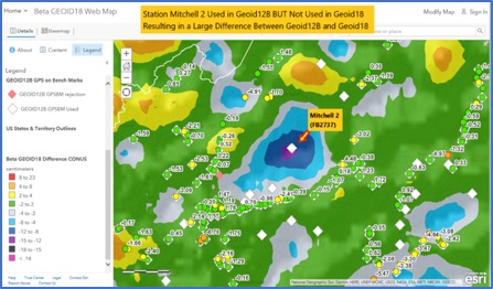
Figure 12. Example of a Large Difference Between Geoid12B and Geoid18 in Western North Carolina (Screenshot: National Geodetic Survey)
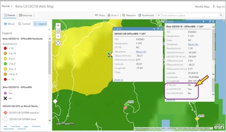
I described the NGS’ published height codes in my October 2016 column. In the case of Mitchell 2, there’s no leveling data in NGS’ database in the area surrounding Mitchell 2. There may be leveling projects that have been performed by other agencies such as the USGS but the leveling data have not been processed and loaded into NGS’ database. Users could help by performing GNSS observations on bench marks in the region that are in NGS’ database and/or by performing leveling observations between the GPS on BMs station and the nearest bench mark that has leveling data in NGS’ database.In the example of a large difference between Geoid12B and Geoid18 in Western North Carolina, station Mitchell 2 (PID FB2737) was used in Geoid12B but not used in Geoid18. It wasn’t used in Geoid18 because the NAVD 88 height was not based on an adjustment. According to the description, the leveling tie was performed by a field party that was performing a horizontal survey project (see Figure 13). The field party performed the appropriate leveling procedures but, in this case, the leveling data have not been placed in computer-readable form, so the orthometric height cannot be verified.
Figure 13. NGS Data Sheet for Station Michell 2 (PID FB2737) (Screenshot: National Geodetic Survey)
I encourage users to access the web map and investigate stations that have large post-modeled residuals and/or stations that were used in Geoid12B but were not used in Geoid18. The NGS analyst rejected stations based on pre- and post-modeled residuals but many times there wasn’t enough redundant information available to ensure the station should be rejected or used in the creation of the hybrid geoid model. Users should be commended for their participation in the GPS on BMs program. Hopefully, users will continue their support by evaluating the beta hybrid geoid model.
My last two columns (NGS 2018 GPS on BMs program in support of NAPGD2022 — Part 6 and NGS 2018 GPS on BMs program in support of NAPGD2022 — Part 7) described the National Geodetic Survey’s (NGS) GPS on BMs 2018 interactive web map, and provided an update and status report on stations observed in support of the 2018 GPS on BMs Program. This column will provide another update and status report on stations observed in support of the 2018 GPS on BMs program and provide an example of how the OPUS-shared results filled in a void area in West Virginia that will benefit the development of the hybrid geoid model GEOID18. The column will also provide an example of how OPUS Shared results identified a reset station that has an invalid NAVD 88 height, and the importance of having a least two OPUS Shared results to ensure the reliability of the OPUS solutions.
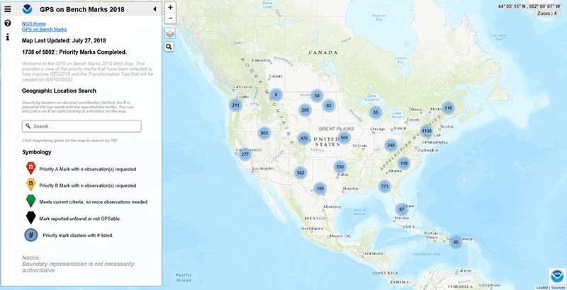
As mentioned in the last column, the GPS on BMs 2018 web page contains a link to a web map where users can determine which bench marks NGS would like users to occupy before the August 31, 2018, deadline. The box titled “2018 Web Map” depicts the map update as of July 27, 2018 (1738 priority marks completed). My last column reported that as of May 29, 2018, there were 1067 priority marks considered completed. During the past two months, 671 more priority stations have been reported completed. This is progress but this still only represents about 30 percent of the priority marks. Hopefully, this will increase dramatically during the month of August. Remember, the cut-off date for data to be included in the creation of the hybrid geoid model GEOID18 is August 31, 2018.
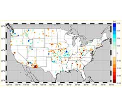
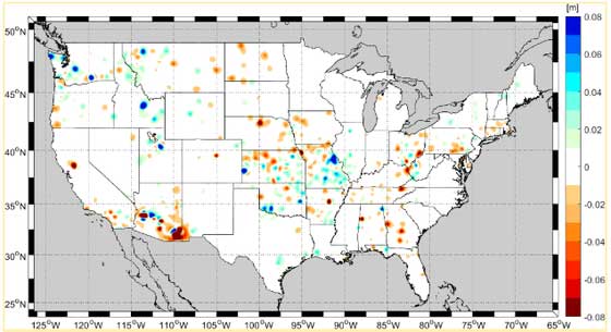
NGS periodically provides an update on the GPS on Bench Marks Program. On July 3, 2018, NGS sent an email to everyone that shared GPS data on NGS bench marks via OPUS or registered for NGS’ February 2018 webinar about GPS on Bench Marks. The email provided an update on the GPS on Bench Marks Program (see box titled “July 3, 2018, NGS Email on GPS on BMs Update”). The map provided in the update indicated that some of the new observations may generate changes between +/- 8 cm.
July 3, 2018, NGS Email on GPS on BMs Update
(Source: Email from National Ocean Service, NOAA; [email protected] to Dave Zilkoski)
Update: GPS on Bench Marks
Over 1,420 marks completed, and two months left to improve GEOID18 accuracy in your area!
Image: National Geodetic SurveyYour observations are making a difference! The color ramp in the map above reflects accuracy improvements in a hybrid geoid model from your recently submitted GPS observations. The improvements will be realized when NGS releases GEOID18.
In case you missed it
In early 2018, NGS released a list of priority bench marks where GPS data is needed to improve GEOID18, NGS’ last planned hybrid geoid model before The North American Vertical Datum of 1988 (NAVD 88) is replaced by the North American-Pacific Datum of 2022 (NAPGD2022). Data to support GEOID18 will be accepted until the end of August 2018. After that, GPS on Bench Marks (GPS on BM) efforts will expand to include other regions and will focus on data to improve future transformation tools.
How can I help?
Following the guidance provided on the NGS GPS on BM website, you can help by collecting static GPS data on adjusted NAVD 88 bench marks and submitting the data to NGS via OPUS Share. To improve efficiency and reduce unnecessary redundancy, we have created a GPS on Bench Marks 2018 web map to help contributors know where we have the data we need and where we still need GPS observations.
Thank you to our contributors
Over 1,700 observations have been submitted to date, completing the required observations for over 1,420 marks from our prioritized list. Each observation requires at least 4 hours of data collection with a survey grade GPS receiver, plus additional time for planning, travel, and data submission, so each one is a significant contribution. Visit the GPS on BM website for updates on our biggest data contributors and each state’s progress toward the goals.
Why are you receiving this email?
• You shared GPS data on NGS bench marks via OPUS, or
• You registered for our February 2018 webinar about GPS on Bench Marks.
We anticipate sending quarterly updates about these and related efforts. If you’d like to opt-out, click the “Manage Subscriptions” at the bottom of this email.
NOAA’s National Geodetic Survey
geodesy.noaa.gov
NGS is tentatively planning another webinar on the GPS on Bench Marks program for August 9, 2018 (2 pm to 3 pm eastern time). NGS will provide an update on the GPS on Bench Mark program and probably will highlight potential improvements between the current hybrid geoid model GEOID12B and the latest prototype version of the future hybrid geoid model GEOID18. I would encourage everyone to sign up for the NGS webinar series.
Source: Plot Generated Using ArcGIS
Users can subscribe to any or all of NGS four public subscription lists — news, webinar, training, and GPS on Bench Marks — by visiting the NGS subscription services web page and submitting their email address for the type(s) of notices they want to receive. (https://www.ngs.noaa.gov/INFO/subscribe.shtml)
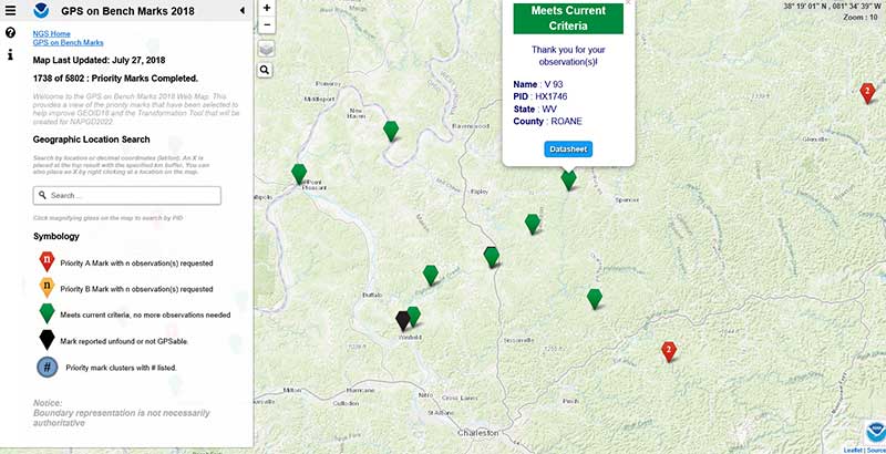
As indicated in the figure provided in NGS’ July 3rd update on the GPS on Bench Marks program email, there are many areas of the country that have already benefitted from users participating in NGS’ GPS on BMs program. This column will highlight an area near Charleston, West Virginia, were users have been very active in providing OPUS Shared results. The box titled “GPS on Bench Marks near Charleston, West Virginia” depicts the marks that meet NGS’ criteria and will be involved in the development of the hybrid geoid model GEOID18. As you can see from the plot, there are several new stations that will be used in the development of the model which will help to improve the reliability of the product.
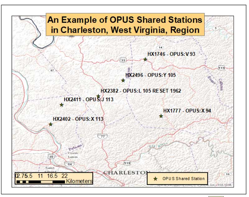
The box titled “An Example of OPUS Shared Stations in Charleston, West Virginia, Region” provides the stations’ PID and OPUS designation. The six OPUS Shared stations cover approximately a 50 km square area. Most of the stations are only 10 km apart. These stations will definitely help to improve the reliability of the hybrid GEOID18 model.
An Example of OPUS Shared Stations in Charleston, West Virginia, region
(Source: Plot Generated Using ArcGIS)
Source: Plot Generated Using ArcGIS
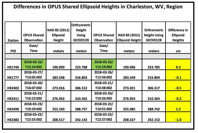
When using OPUS Shared results, users should always check to see if a station has been observed more than once. The box tilted “Differences in OPUS Shared Ellipsoid Heights in Charleston, WV, Region” lists the pairs of OPUS observations for the stations depicted in the previous plot. The column labeled “Difference in Ellipsoid Heights” provides the differences in ellipsoid heights based on the two different OPUS Shared results. All differences are less than 1.5 cm and most are less than 1.0 cm. This is indicating good repeatability to the cm level but this may not be indicating accuracy. These stations were observed one day apart but observed at about the same time of the day. They could have the same systematic errors effecting the results such as multipathing and satellite geometry. When performing the second OPUS Shared observation, users should select a different time of day to improve the chances of detecting, reducing, and/or eliminating the effects of remaining systematic errors.
Differences in OPUS Shared Ellipsoid Heights in Charleston, West Virginia, region
Source: National Geodetic Survey
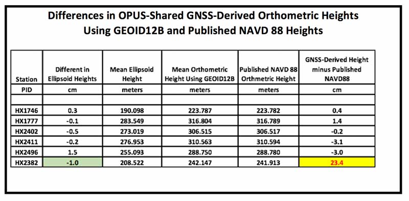
The box titled “Differences in OPUS-Shared GNSS-Derived Orthometric Heights Using GEOID12B and Published NAVD 88 Heights” provides the differences between the GNSS-derived orthometric heights using GEOID12B and the published NAVD 88 values. This table indicates that there is a large difference (23.4 cm) for station HX2382 (L105 Reset 1962). Since the two ellipsoid heights only differ by 1.0 cm, this is an indication that the station probably moved since it was Reset or the reset observations were performed incorrectly. Either way, this station should not be used in the development of the hybrid model or used by anyone for geodetic control.
Differences in OPUS-Shared GNSS-Derived Orthometric Heights using GEOID12B and Published NAVD 88 Heights
Source: National Geodetic Survey
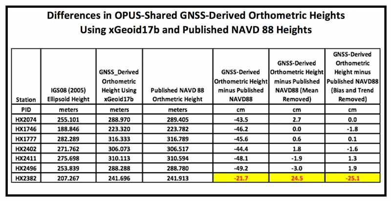
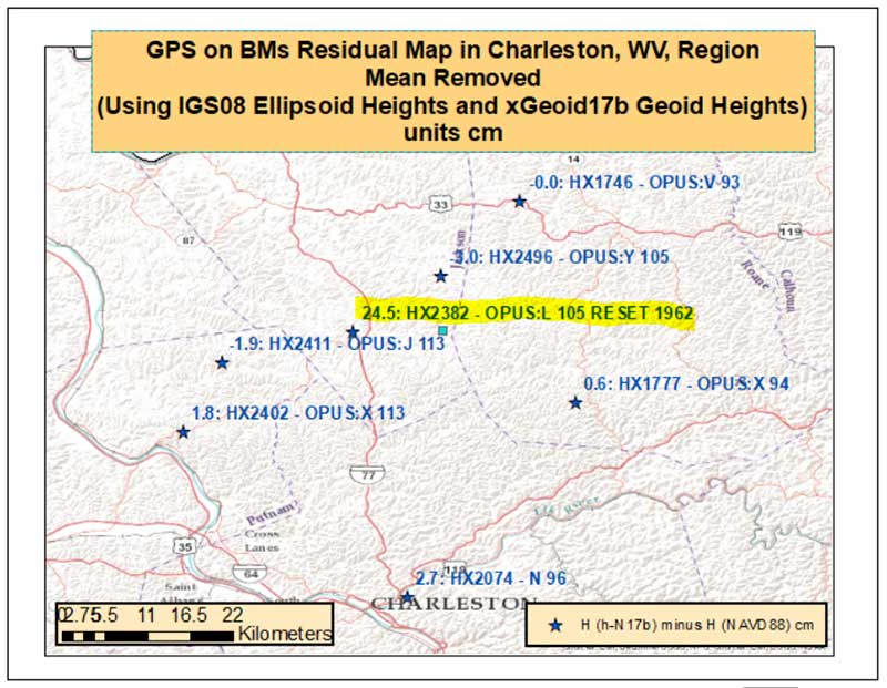
Since GEOID12B is a hybrid geoid model that was designed to be consistent with NAVD 88 values, I always compute differences between GNSS-derived orthometric heights using the experimental geoid model and published NAVD 88 height values. I described this process in my October 2015 column (http://stage.globalpositioningnews.com/establishing-orthometric-heights-using-gnss-part-3/). The box titled “Differences in OPUS-Shared GNSS-Derived Orthometric Heights Using xGeoid17b and Published NAVD 88 Heights” provides the differences between the GNSS-derived orthometric heights estimated using IGS08 (2005) ellipsoid heights with the xGeoid17b geoid model and published NAVD 88 heights. The values in the column labeled “GNSS-Derived Orthometric Height minus Published NAVD 88” represent an approximate difference between NAPGD2022 and NAVD 88. The box titled “OPUS-Shared GNSS-Derived Orthometric Heights Using xGeoid17b minus Published NAVD 88 Heights” provides a plot that depicts these differences.
Differences in OPUS-Shared GNSS-Derived Orthometric Heights Using xGeoid17b and Published NAVD 88 Heights
Source: National Geodetic Survey
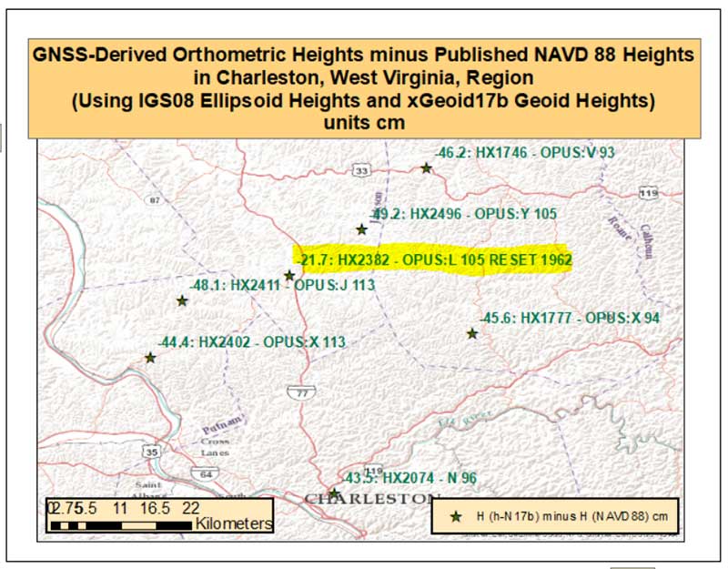
OPUS-Shared GNSS-Derived Orthometric Heights Using xGeoid17b minus Published NAVD 88 Heights
(Source: Plot Generated Using ArcGIS)
Source: Plot Generated Using ArcGIS
Once again, it should be noted that PID HX2382 value is much different from the other values. To look for outliers, a mean difference was removed from the results. The box titled “OPUS-Shared GNSS-Derived Orthometric Heights Using xGeoid17b minus Published NAVD 88 Heights with a Mean Value Removed” makes it easier to see that station HX2382 is an outlier. The station is approximately 25 cm different from its neighboring stations that are only 10 km away. As previously mentioned, this station apparently moved since being Reset in 1962 or the reset observations were performed incorrectly. Identifying stations that have moved since the last time they have been leveled is one of the benefits of participating in the GPS on BMS program.
OPUS-Shared GNSS-Derived Orthometric Heights Using xGeoid17b minus Published NAVD 88 Heights with a Mean Value Removed
(Source: Plot Generated Using ArcGIS)
Source: Plot Generated Using ArcGIS
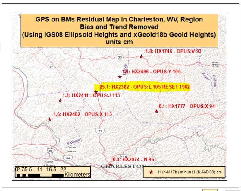
For completeness, both a bias and trend were removed from the differences since IGS08 (2005) GNSS-derived orthometric heights and NAVD 88 heights indicate that there’s an apparent long-wavelength trend between the two sets of values. The box titled “OPUS-Shared GNSS-Derived Orthometric Heights Using xGeoid17b minus Published NAVD 88 Heights with Bias and Trend Removed” depict the differences with a bias and trend removed. As in the other figures, PID HX2382 clearly indicates that it is an outlier relative to its neighbors. This station would be rejected by the geoid team when creating the next hybrid geoid model.
It should be noted that except for the Reset station, all of the differences are less than 2 cm. Although, some relative differences between closely-spaced stations approach 4 cm. For example, the differences between stations HX1746 and HX2496 is -3.7 cm (-1.8 cm – 1.9 cm). The differences in ellipsoid heights from the OPUS Shared solutions are all less than 1.5 cm, even the differences between ellipsoid heights for station HX2382 is only 1 cm. This is an indication that the reset station, HX2382, does not have a valid NAVD 88 published height and should not be used as control. Surveyors that adhere to the FGCS specifications and procedures would realize that this station did not have a valid NAVD 88 height and would not use the published NAVD 88 as control in their project. For example, surveyors performing a leveling project would perform a 2- or 3- mark leveling tie and the results would indicate that the station had moved since it was last leveled.
OPUS-Shared GNSS-Derived Orthometric Heights Using xGeoid17b minus Published NAVD 88 Heights with Bias and Trend Removed
(Source: Plot Generated Using ArcGIS)
Source: Plot Generated Using ArcGIS
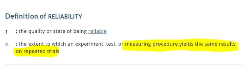
This type of validation procedure should also apply for OPUS users. If a user obtains one OPUS solution and proceeds to perform a survey from that station, the user does not know whether the OPUS height value is reliable or accurate. One solution does not provide any indication of reliability.
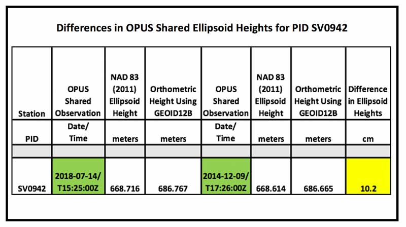
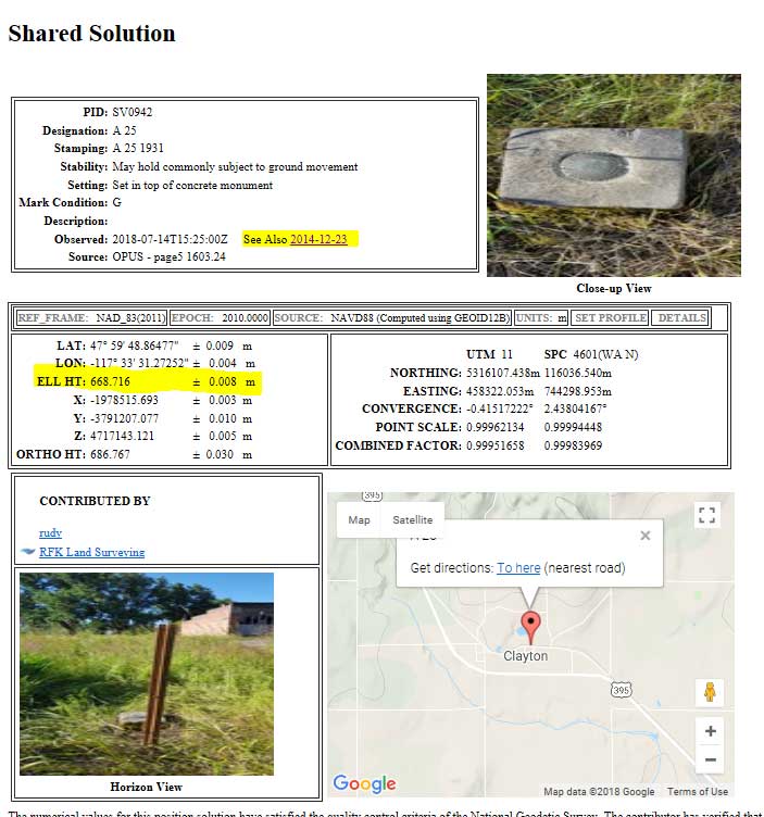
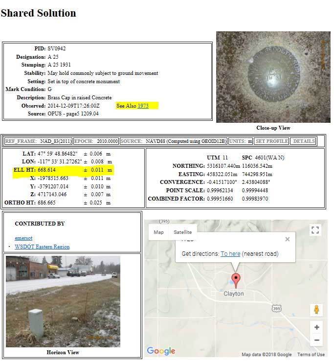
The OPUS Shared station PID SV0942 (A 25) is an example of two OPUS Shared results generating ellipsoid height values that differ by 10 cm. (See yellow highlighted section in the box titled “Differences in OPUS Shared Ellipsoid Heights for PID SV0942.”) This large difference is significant when you performing a survey where you need heights to better than 3 cm (0.1 foot). This is one reason that NGS requires two OPUS Shared solution for every mark used in the development of the hybrid geoid model.
Differences in OPUS Shared Ellipsoid Heights for PID SV0942
Source: National Geodetic Survey
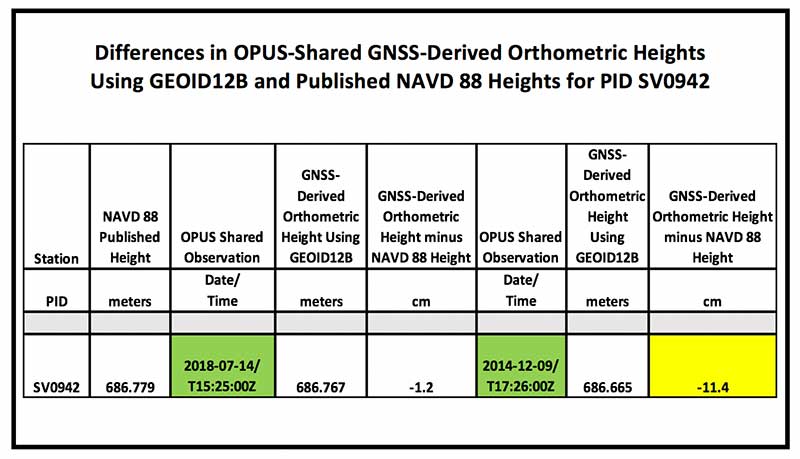
In the OPUS Shared solutions of PID SV0942, the latest OPUS Shared GNSS-derived orthometric heights (2018-07-14) agrees to about a cm with the published NAVD 88 height, while the 2014 Opus Shared GNSS-derived orthometric height is -11.4 cm different from the published NAVD 88 value. (See yellow highlighted section in box titled “Differences in OPUS-Shared GNSS-Derived Orthometric Heights Using GEOID12B and Published NAVD 88 Heights for PID SV0942.”)
Differences in OPUS-Shared GNSS-Derived Orthometric Heights Using GEOID12B and Published NAVD 88 Heights for PID SV0942
Source: National Geodetic Survey
It should be noted that the error estimates provided in the Opus Shared output indicate the ellipsoid heights are good to about +/- 1 cm. (See highlighted section in box titled “Two OPUS Shared Solution for PID SV0942.”) Saying that, the two NAD 83 (2011) ellipsoid heights disagree with each other by 10.2 cm. I like a quote that is attributed to Mark Twain – “It ain’t what you don’t know that gets you into trouble. It’s what you know for sure that just ain’t so.” (Obtained from http://lukefostvedt.com/famous-quotes-about-statistics/). I’m not suggesting that Opus Shared solutions results are incorrect. I’m attempting to provide an example of why users need to repeat all observations and to demonstrate how error estimates can be misleading.
“It ain’t what you don’t know that gets you into trouble.It’s what you know for sure that just ain’t so.”
The number of GPS on Bench Mark stations completed as of July 27, 2018, represents about 30 percent of the total number of stations that need to be observed. As I have explained in previous columns, there are many invalid GPS on BMs stations that may be used in the next hybrid geoid model unless more bench marks with valid NAVD 88 heights are observed with GNSS. NGS will accept data for inclusion in the next hybrid geoid model, GEOID18, until the end of August 2018. After that, NGS’ GPS-on-Bench-Mark Program will expand to include other regions and will focus on data to improve NGS datum transformation tools. This column provided an update and status report on stations observed in support of the 2018 GPS on BMs program, provided an example of how the OPUS Shared results can be used to identify a station that may have moved since it was last leveled, and the importance of repeating OPUS observations. I would encourage users to register for NGS’ next webinar on the GPS on Bench Mark Program scheduled for Thursday, Aug. 9th to hear the latest status of the program.
These columns have focused on procedures and routines for establishing GNSS-derived orthometric heights. There are many ways to analyze and investigate GNSS data and adjustment results. I have provided some basic concepts that I believe are important for users to understand.
The selection of constraints is a very important part of establishing accurate and consistent NAVD 88 GNSS-derived orthometric heights. All of the analysis and recommendations have been based on using the National Geodetic Survey‘s latest scientific geoid model.
I recommend first performing the analysis using the scientific geoid model because the hybrid geoid model has been warped to be consistent with the published NAVD 88 values. However, as mentioned in Part 7 (June 2016), in practice, GNSS-derived orthometric heights are incorporated into the NAVD 88 using the latest hybrid geoid model GEOID12B. This column will focus on the NGS “GPS on BMS (GPSBM)” dataset that was used to create the hybrid geoid model.
As mentioned in Part 3 (October 2015), the hybrid geoid model is designed to fit the published NAVD 88 leveling-derived orthometric heights. Saying that, the GPSBM dataset can be used to identify potential issues in the NAVD 88 published orthometric heights. GNSS users should be familiar with this dataset and how it can be used in their analysis. This column will provide tools and routines that can be used to identify potential issues in NAVD 88 heights and/or NAD83 (2011) published ellipsoid heights.
Each of the below regions uses variants of the NAD 83 reference frame and a local vertical datum. Several versions of NAD 83 exist conforming to significant plates: Pacific, Mariana, and North America. Likewise, each region has its own vertical datum. It is not possible to level across water, so islands will have selected a tide gauge to serve as the local datum point and all leveling is tied to that site. The only exception to this is Hawaii. No tide gauge was selected in the Hawaiian Islands and no vertical datum has been established as of yet. Hence, GEOID12B in Hawaii transforms between NAD 83 (PA11) and the same geopotential (geoid) surface as the USGG2012 model ( W0 = 62636856.00 m**2/s**2).
Items that are listed in the below table include the final GPSBM files for each region as both Excel spreadsheets and text files as well as thumbnail images linked to larger images showing the distribution of the GPSBM’s. Alaska and the island regions are more consistent, so not many points were dropped and each is provided in its own spreadsheet/text file and identified with the appropriate ellipsoidal reference frame and level datum (see below).
The most significant work occurred in the COnterminous United States (CONUS). For CONUS, there were 24,782 points with 911 rejected leaving 23,961. These were supplemented from the OPUS-database with 737 points of which 238 were rejected leaving 499. There were also 579 points in Canada with 5 rejected leaving 574. In Mexico, there 744 of which 497 were clipped since they were too far south and another 70 were rejected leaving 177. This brings a total of 26,932 points of which 1,721 were rejected or clipped and 25,211 retained for modeling GEOID12B. The data in Canada and Mexico provide continuity up to and across the U.S. borders but do not make the GEOID12B model valid in those countries.
Points were rejected either because the State Advisor recommended it be dropped (e.g., known subsidence region), the residual ellipsoid height errors (from the NA2011 project) indicated a point was too noisy in comparison to other points in a state/region, the orthometric height was suspect, or the residual errors during geoid modeling were too high. The corresponding error flags are ‘S’, ‘h’, ‘H’, and ‘N’ as seen on the spreadsheet and text files. These points then represent the control data that were used to define the transformation between NAD 83 and NAVD 88 for CONUS.
The control data were much simpler in other regions due to the lack of quantity (more than two orders of magnitude less). Data in these regions follows a similar pattern where some data are rejected based on the codes given above for CONUS. The columns on the right side give the respective datums realized by GEOID12B for each region.
Table 1 is an excerpt of the excel spreadsheet for the GPSBM dataset and provides a sample of the contents. The headings of the columns are fairly self-explanatory. What’s important here is that the excel spreadsheet provides the name, latitude, longitude, NGS’ PID, the ellipsoid height and orthometric height of the stations used in making GEOID12B.
Table 1
Excerpt of the Excel spreadsheet for GPS on benchmarks (GPSBM) used to make GEOID12B.
The “GPS On Bench Marks (GPSBM) Used To Make GEOID12B” write up states that 1,721 stations were rejected and were not used in developing the hybrid geoid model. It also states that for the conterminous United States (CONUS), there were 24,782 stations with 911 rejected leaving 23,961. This column is going to focus on CONUS but the analysis can be performed everywhere.
As the write up states, stations were rejected for four different reasons:
Code h – The residual ellipsoid height errors from the NAD 83 (2011) project indicated that the point was too noisy,
Code H – The orthometric height was suspect,
Code N – The residual errors during geoid modeling were too high.
These rejected stations were not used to make the hybrid geoid model but since the hybrid geoid model is distorted to fit the NAVD 88, these rejected stations as well as stations nearby the rejected stations should be re-evaluated using the latest scientific geoid model, e.g. xGeoid16b.
So, what should the user do with the GPSBM table? I recommend that users perform the following steps when analyzing the stations in the GPSBM table.
Step 1: Compare the modeled GEOID12B (N12B) value to the computed GPS/Leveling (h minus H) value using the following formula: Published N12B from the NGS data sheet minus (ellipsoid height from the GPSBM table minus orthometric height from the GPSBM table). We discussed this procedure a year ago in Part 3 (October 2015). It should be noted that the orthometric height in the GPSBM table may be different than the published NAVD 88 height on the NGS data sheet if the station has been readjusted since the GPSBM table was created.
Step 2: Repeat the procedure in Step 1 using the latest NGS experimental geoid model, e.g. xGeoid16b. At this time, NGS only provides the experimental geoid models referenced to IGS08 so the user will have to use NGS’ xGeoid16 web tool to obtain the station’s IGS08 ellipsoid height and xGeoid16b value. The input to the tool is the station’s NAD 83 (2011) coordinates (latitude, Longitude, and ellipsoid height). [An example of using the xGeoid16 web tool is provided in the box titled “Example of Using NGS xGeoid16 Web Tool.”] As discussed in Part 3 (October 2015), the user will have to remove a bias and trend based on the differences in the region.
The user could also transform xGeoid16b/IGS08 geoid values to xGeoid16b/NAD 83 (2011) geoid values using their own tools, and then remove a bias and trend based on the differences. Michael Dennis, a PhD candidate at Oregon State University, created an ArcGIS raster of the xGeoid16b model, where his model has been referenced to NAD 83 (Michael L. Dennis, RLS, PE, MS Civil Eng., Geodetic Analysis, LLC, 55 Creek Rock Road, Sedona, AZ 86351). He removed a trend using the GPS/Leveling data set as input; therefore, this raster file is a form of a hybrid geoid model distorted only to remove the tilt assumed to be in the NAVD 88. I will refer to this model as Geoid16B_NAD83 to avoid confusion with NGS’ xGeoid16b model.
*Orthometric height difference between xGEOID16B to model shown
Step 3: Use the station’s data sheet to identify how the station’s orthometric height was determined; for example, was it rigorously adjusted into the NAVD 88 (published height attribute – Adjusted). We discussed the attributes of the NGS data sheet in Part 5 (February 2016). A summary of the attributes from the NGS data sheet DSDATA.TXT file is provided in the box titled “Extracted from NGS’ DSDATA.TXT.” I have highlighted the most common attributes of the stations involved in making GEOID12B.
Extracted from NGS’ DSDATA.TXT
***************************************************************************
* dsdata.txt *
***************************************************************************
There are various Vertical Control sources, as specified below:ADJUSTED = Direct Digital Output from Least Squares Adjustment of Precise Leveling.
(Rounded to 3 decimal places.)ADJ UNCH = Manually Entered (and NOT verified) Output of Least Squares Adjustment of Precise Leveling.
(Rounded to 3 decimal places.)
POSTED = Pre-1991 Precise Leveling Adjusted to the NAVD 88 Network After Completion of the NAVD 88 General Adjustment of 1991.
(Rounded to 3 decimal places.)
READJUST = Precise Leveling Readjusted as Required by Crustal Motion or Other Cause.
(Rounded to 2 decimal places.)
N HEIGHT = Computed from Precise Leveling Connected at Only One Published Bench Mark.
(Rounded to 2 decimal places.)
RESET = Reset Computation of Precise Leveling.
(Rounded to 2 decimal places.)
COMPUTED = Computed from Precise Leveling Using Non-rigorous Adjustment Technique.
(Rounded to 2 decimal places.)
GPSCONLV = Leveled Orthometric Height tied to GPS HT_MOD Orthometric Height.
(Rounded to 2 decimal places.)
LEVELING = Precise Leveling Performed by Horizontal Field Party.
(Rounded to 2 decimal places.)
H LEVEL = Level between control points not connected to bench mark.
(Rounded to 1 decimal places.)
GPS OBS = Computed from GPS Observations.
(Rounded to 1 decimal places.)
VERT ANG = Computed from Vertical Angle Observations.
(Rounded to 1 decimal place; If No Check, to 0 decimal places.)
SCALED = Scaled from a Topographic Map.
(Rounded to 0 decimal places.)
U HEIGHT = Unvalidated height from precise leveling connected at only one NSRS point.
(Rounded to 2 decimal places.)
VERTCON = The NAVD 88 height was computed by applying the VERTCON shift value to the NGVD 29 height.
(Rounded to 0 decimal places.)
Step 4: Use the station’s NGS data sheet to determine the adjustment date of the station’s published NAVD 88 orthometric height. We discussed this in Part 7 (June 2016). As mentioned in Part 7, if the station has a different adjustment date than other stations nearby, there could be inconsistencies due to adjustment distribution corrections and/or movement.
Step 1 was demonstrated in Part 3 (October 2015) so we don’t need to describe the process in this column. Comparing published GEOID12B values with computed values is the first step; the difference is an indication of how well the data fit the model and can be useful for identifying large outliers. It can be helpful in prioritizing where additional observation should be obtained when there are limited resources. Provided below is an example of where to obtain the information for comparing the modeled GEOID12B (N12B) value to the computed GPS/Leveling (h minus H) value using the following formula: Published N12B from the NGS data sheet minus (ellipsoid height from the GPSBM table minus orthometric height from the GPSBM table). The user can obtain the GEOID12B value from the NGS data sheet [see box titled “Excerpt from NGS Data Sheet For Station L 275 (HW2088)”]; for this example, the GEOID12B value for station L 275 is -30.813 m. Table 2 is an excerpt from the GPSBM file that contains the ellipsoid height (599.253 m) and the orthometric height (630.016 m) for station L 275. It should be noted that the ellipsoid and orthometric heights in the GPSBM table are given in millimeters. The first row of table 3 provides the results of the computation: [-30814 mm – (599253 mm – 630016m m) = 51 mm], or 5.1 cm.
Table 2
Excerpt of the Excel spreadsheet for GPS on benchmarks (GPSBM) used to make GEOID12B – Stations on plots in this column.
Excerpt from NGS Data Sheet For Station L 275 (HW2088)
PROGRAM = datasheet95, VERSION = 8.9.1
1 National Geodetic Survey, Retrieval Date = OCTOBER 1, 2016
HW2088 ***********************************************************************
HW2088 CBN – This is a Cooperative Base Network Control Station.
HW2088 DESIGNATION – L 275
HW2088 PID – HW2088
HW2088 STATE/COUNTY- WV/RANDOLPH
HW2088 COUNTRY – US
HW2088 USGS QUAD – MILL CREEK (1995)
HW2088
HW2088 *CURRENT SURVEY CONTROL
HW2088 ______________________________________________________________________
HW2088* NAD 83(2011) POSITION- 38 43 54.95105(N) 079 58 19.75931(W) ADJUSTED
HW2088* NAD 83(2011) ELLIP HT- 599.253 (meters) (06/27/12) ADJUSTED
HW2088* NAD 83(2011) EPOCH – 2010.00
HW2088* NAVD 88 ORTHO HEIGHT – 630.016 (meters) 2066.98 (feet) ADJUSTED
HW2088 ______________________________________________________________________
HW2088 NAD 83(2011) X – 867,581.099 (meters) COMP
HW2088 NAD 83(2011) Y – -4,906,352.726 (meters) COMP
HW2088 NAD 83(2011) Z – 3,969,521.039 (meters) COMP
HW2088 LAPLACE CORR – 0.13 (seconds) DEFLEC12B
HW2088 GEOID HEIGHT – -30.814 (meters) GEOID12B
HW2088 DYNAMIC HEIGHT – 629.553 (meters) 2065.46 (feet) COMP
HW2088 MODELED GRAVITY – 979,873.5 (mgal) NAVD 88
HW2088
HW2088 VERT ORDER – FIRST CLASS II
HW2088
HW2088 Network accuracy estimates per FGDC Geospatial Positioning Accuracy
HW2088 Standards:
HW2088 FGDC (95% conf, cm) Standard deviation (cm) CorrNE
HW2088 Horiz Ellip SD_N SD_E SD_h (unitless)
HW2088 ——————————————————————-
HW2088 NETWORK 1.00 1.94 0.45 0.36 0.99 -0.05669181
Table 3 contains the comparisons between modeled geoid values and their computed geoid values for five station pairs that have large relative differences. Looking at table 3 one can see that there are several large relative differences between the published GEOID12B model and computed geoid model (see column titled “N12B minus (h-H)” in table 3). This doesn’t mean that the model is incorrect, it only means that there were large relative differences that the model had to account for. As previously mentioned, GEOID12B was created to be consistent with the NAVD 88.
Since the experimental geoid model xGeoid16b_NAD is not distorted to conform to the NAVD 88 everywhere, it should provide better information for identifying outliers and determining which stations appear to be inconsistent with its neighbors.
Figure 1 – All GPS on BMS Residuals Using Geoid16b_NAD model (note: rejections by geoid team have been removed).
Table 3
Table of selected stations involving large relative differences depicted in plots in this column.
(Results are provided for GEOID12B and Geoid16B_NAD Models*) *Michael Dennis, a Ph.D. candidate at Oregon State University, created the xGEOID16B ArcGIS raster, where the model has been referenced to NAD 83 with a trend and bias added to account for the apparent tilt in the NAVD 88. This model is denoted as Geoid16B_NAD (N16b) in this column.
Figure 1 is a plot of all of the GPSBM residuals using the Geoid16B_NAD83 model. This plot indicates that there are a lot of large residuals. First, let’s define what I’m calling residuals. The residuals on my plots are the differences between the modeled geoid height value and the computed geoid height value using the ellipsoid height (h) and orthometric height (H) from the GPSBM data set; that is, residual = modeled gravity value – (h minus H). The largest negative residual is -37.3 cm and the largest positive residual is 33.8 cm.
Figure 2 – Positive GPS on BMS Residuals Using Geoid16b_NAD model (note: rejections by geoid team have been removed).
Figure 2 is a plot of the positive GPS on BMS residuals using Geoid16b_NAD geoid model. There are 5957 residuals greater than 5 cm (not including the stations rejected by the NGS geoid team). As you can see, it appears that most of the positive residuals are on the eastern half of the United States.
Figure 3 – Negative GPS on BMS Residuals Using Geoid16b_NAD model (note: rejections by geoid team have been removed).
Figure 3 is a plot of the negative GPS on BMS residuals using Geoid16b_NAD geoid model. There are 4113 residuals less than -5 cm (not including the stations rejected by the NGS geoid team). As you can see from the plot, the negative residuals appear to be more evenly distributed across the United States than the positive residuals. It does, however, appear that there are more negative residuals greater than -5 cm along the Gulf Coast, Atlantic Coast, and the Great Lakes than there are positive residuals greater than 5 cm. In addition, there appears to be a lot of negative residuals in the northeastern United States.
Figure 4 – GPS on BMS Residuals Using Geoid16b_NAD model in North Carolina and South Carolina (note: rejections by geoid team have been removed).
Figure 4 is a plot of the GPS on BMS residuals using the Geoid16b_NAD geoid model in the North Carolina and South Carolina border region. What’s interesting about this plot is that South Carolina doesn’t seem to have many negative residuals where North Carolina has both negative and positive residuals. We will look at this in more detail later in this column.
Figure 5 – GPS on BMS Residuals Using Geoid16b_NAD model in Washington and Oregon Region (note: rejections by geoid team have been removed).
Figure 5 is a plot of the GPS on BMS residuals using Geoid16b_NAD model in the Washington and Oregon Region. This graphic shows some large grouping of negative and positive residuals, especially along the Pacific Coast in Northwestern Washington State.
Now, let’s look at some large relative differences in residuals between stations that are spatially close together. Figure 6 is a plot of large relative differences between groups of GPS on BMS residuals (using Geoid16b_NAD model) at the North Carolina/South Carolina border. In figure 6, two stations (FA1337 and FA1560) are about 20 km apart and the difference in residuals is -18.6 cm (-12.4 cm minus 6.2 cm). This is a large difference for only 20 km. What is even more significant is that the group of stations near FA1337 are all negative residuals (around -10 cm) and the group of stations near FA1560 are all positive residuals (around 6 cm), this could be an indication of a large distribution correction due to the NAVD 88 design. We discussed the distribution correction in Part 7 (June 2016). These stations definitely needs to be investigated.
The next step in my process is to look at the NGS data sheets for these stations to determine how the stations were adjusted.
Step 3: Look at the station’s data sheet to identify how the station’s orthometric height was determined; for example, was it rigorously adjusted into the NAVD 88 (published height attribute is “Adjusted”) or was it determined by precise leveling performed by horizontal field party (published height attribute is “Leveling”).
The data sheet for station FA1337 states that the NAVD 88 attribute code is “GPS OBS.” [See box titled “Excerpt from NGS Data Sheet for PID FA1337.”] The data sheet for FA1560 states that the NAVD 88 attribute code is “Adjusted.” The orthometric height on the GPSBM file is different than the current published NAVD 88 orthometric height for station FA1337 (See table 3). This station’s leveling-derived orthometric height was superseded by a GNSS-derived orthometric height. Saying that, the GPSBM file only uses leveling-derived orthometric heights; therefore, stations that have been superseded by GNSS surveys are still included in the GPSBM file but their original published leveling-derived height is used for the analysis. Table 3 provides the orthometric height for FA1337 that was used in making GEOID12B. As previously mentioned, stations may be rejected by the geoid team based on the criteria outlined in the beginning of this column. Saying that, neither of the two stations were rejected by the NGS geoid team. This implies that the stations were consistent with their neighbors as far as the geoid model was concerned. Figure 6 confirms that all the stations around FA1337 and FA1560 are consistent with each other based on the Geoid16b_NAD geoid model. The fact that the two groups differ by 18 6 cm needs to be investigated.
Excerpt from NGS Data Sheet for PID FA1337
PROGRAM = datasheet95, VERSION = 8.9.1
1 National Geodetic Survey, Retrieval Date = OCTOBER 3, 2016
FA1337 ***********************************************************************
FA1337 HT_MOD – This is a Height Modernization Survey Station.
FA1337 DESIGNATION – RU 36
FA1337 PID – FA1337
FA1337 STATE/COUNTY- NC/RUTHERFORD
FA1337 COUNTRY – US
FA1337 USGS QUAD – FOREST CITY (1993)
FA1337
FA1337 *CURRENT SURVEY CONTROL
FA1337 ______________________________________________________________________
FA1337* NAD 83(2011) POSITION- 35 18 08.14237(N) 081 51 17.93516(W) ADJUSTED
FA1337* NAD 83(2011) ELLIP HT- 249.869 (meters) (06/27/12) ADJUSTED
FA1337* NAD 83(2011) EPOCH – 2010.00
FA1337* NAVD 88 ORTHO HEIGHT – 281.79 (meters) 924.5 (feet) GPS OBS
FA1337 ______________________________________________________________________
Figure 6 – GPS on BMS Residuals: Large Relative Differences Between a Group of Stations at the North Carolina/South Carolina Border (note: rejections by geoid team have been removed)
Figure 7 is a plot of the GPS on BMS residuals using Geoid16b_NAD that depicts a large difference between two stations only 20 km apart near the Maryland/West Virginia border. I will use this station pair to demonstrate the next step in my process.
Step 4 is to use the station’s NGS data sheet to determine the adjustment date the of station’s published NAVD 88 orthometric height.
The NAVD 88 attribute on the NGS data sheet states that both of these stations are coded as “Adjusted” but station JW0639 adjustment date is April 1995 (see box titled “excerpt from NGS Data Sheet for PID JW0639”) and JW1296 adjustment date was in June 1991 (the General Adjustment of NAVD 88). These large relative differences could be due to inconsistencies between adjusted heights due to the adjustment distribution corrections and/or constraints imposed in the April 1995 adjustment. Bench marks near the stations should be observed to determine if the same large relative difference exists, and the 1995 NAVD 88 adjustment project report should be reviewed to determine if a large distribution correction was applied.
Excerpt from NGS Data Sheet for PID JW0639
1 National Geodetic Survey, Retrieval Date = OCTOBER 3, 2016
JW0639 ***********************************************************************
JW0639 CBN – This is a Cooperative Base Network Control Station.
JW0639 DESIGNATION – J 17 RESET
JW0639 PID – JW0639
JW0639 STATE/COUNTY- MD/GARRETT
JW0639 COUNTRY – US
JW0639 USGS QUAD – ACCIDENT (1994)
JW0639
JW0639 *CURRENT SURVEY CONTROL
JW0639 ______________________________________________________________________
JW0639* NAD 83(2011) POSITION- 39 37 53.59739(N) 079 18 57.44776(W) ADJUSTED
JW0639* NAD 83(2011) ELLIP HT- 701.266 (meters) (06/27/12) ADJUSTED
JW0639* NAD 83(2011) EPOCH – 2010.00
JW0639* NAVD 88 ORTHO HEIGHT – 732.713 (meters) 2403.91 (feet) ADJUSTED
JW0639 ______________________________________________________________________
*
*
*
JW0639
JW0639.The orthometric height was determined by differential leveling and
JW0639.adjusted by the NATIONAL GEODETIC SURVEY
JW0639.in April 1995.
JW0639
Figure 7 – GPS on BMS Residuals Using Geoid16b_NAD: Large Relative Difference Between Stations About 20 km Apart Along MD/WV Border (note: rejections by geoid team have been removed).Figure 8 – GPS on BMS Residuals Using Geoid16b_NAD: Large relative Difference Between Stations 15 km Apart in Randolph County, West Virginia (note: rejections by geoid team have been removed).
Figure 8 is a plot of GPS on BMS residuals using Geoid16b_NAD that depicts a large relative difference between stations 15 km apart in Randolph County, West Virginia. This plot involves station HW3677 which has a published NAVD 88 attribute of “Leveling.” (See box titled “Excerpt from NGS Data Sheet for PID HW3677.”) The excerpt from the data sheet has the following statement: “The orthometric height was determined by differential leveling. The vertical network tie was performed by a horz. field party for horz. obs reductions. Reset procedures were used to establish the elevation.”
It would be useful if stations near this station were observed by GNSS surveys to determine what is occurring in this region.
Excerpt from NGS Data Sheet for PID HW3677
1 National Geodetic Survey, Retrieval Date = OCTOBER 2, 2016
HW3677 ***********************************************************************
HW3677 DESIGNATION – GPS 1
HW3677 PID – HW3677
HW3677 STATE/COUNTY- WV/RANDOLPH
HW3677 COUNTRY – US
HW3677 USGS QUAD – MILL CREEK (1995)
HW3677
HW3677 *CURRENT SURVEY CONTROL
HW3677 ______________________________________________________________________
HW3677* NAD 83(2011) POSITION- 38 37 50.21531(N) 079 55 29.64175(W) ADJUSTED
HW3677* NAD 83(2011) ELLIP HT- 1129.355 (meters) (06/27/12) ADJUSTED
HW3677* NAD 83(2011) EPOCH – 2010.00
HW3677* NAVD 88 ORTHO HEIGHT – 1159.91 (meters) 3805.5 (feet) LEVELING
HW3677 ______________________________________________________________________
*
*
*
*
HW3677 HW3677.The orthometric height was determined by differential leveling.
HW3677.The vertical network tie was performed by a horz. field party for horz.
HW3677.obs reductions. Reset procedures were used to establish the elevation.
HW3677
Figure 9 is a GPS on BMS residual plot of large relative stations about 30 km apart in Wasco County, Oregon. This plot has two stations with large differences and both stations have the NAVD 88 attribute of “Adjusted.” Their NGS data sheet states that they were both established in the general adjustment of NAVD 88 in June 1991. In this particular case, the leveling in this region is very old. As described in Part 7 (June 2016), you can retrieve all project identifiers for those projects with observations to or from a station using the station’s PID. The output from the NGS Data Sheet Mark Source Routine for PID RC1228 is shown in the box titled “Output from NGS Data Sheet Mark Source Routine.”
Output from NGS Data Sheet Mark Source Routine
Program: mark_sources Version: 3.0 Date: May 1, 2013RC1228OR/065 J 108
———————————————————-
GPS_OBS
———–
GPS_OBS FORE_POINT in GPS1655
DIR_OBS
———–
DIST_OBS
———–
VERT_OBS
———–
LEV_OBS
———–
LEVEL_OBS
———–
LEVEL_OBS STAND_POINT in L3410
LEVEL_OBS FORE_POINT in L3410***********************************************************
Figure 9 – GPS on BMS Residuals Using Geoid16b_NAD: Large relative stations about 30 km apart in Wasco County, Oregon (note: rejections by geoid team have been removed).
Figure 9 is a GPS on BMS residual plot of large relative stations about 30 km apart in Wasco County, Oregon. This plot has two stations with large differences and both stations have the NAVD 88 attribute of “Adjusted.” Their NGS data sheet states that they were both established in the general adjustment of NAVD 88 in June 1991. In this particular case, the leveling in this region is very old. As described in Part 7 (June 2016), you can retrieve all project identifiers for those projects with observations to or from a station using the station’s PID. The output from the NGS Data Sheet Mark Source Routine for PID RC1228 is shown in the box titled “Output from NGS Data Sheet Mark Source Routine.”
Excerpt from NGS Data Sheet for PID RC1228
PROGRAM = datasheet95, VERSION = 8.9.1
1 National Geodetic Survey, Retrieval Date = OCTOBER 2, 2016
RC1228 ***********************************************************************
RC1228 DESIGNATION – J 108
RC1228 PID – RC1228
RC1228 STATE/COUNTY- OR/WASCO
RC1228 COUNTRY – US
RC1228 USGS QUAD – WAPINITIA (1996)
RC1228
RC1228 *CURRENT SURVEY CONTROL
RC1228 ______________________________________________________________________
RC1228* NAD 83(2011) POSITION- 45 06 49.69715(N) 121 19 19.81396(W) ADJUSTED
RC1228* NAD 83(2011) ELLIP HT- 624.596 (meters) (06/27/12) ADJUSTED
RC1228* NAD 83(2011) EPOCH – 2010.00
RC1228* NAVD 88 ORTHO HEIGHT – 646.140 (meters) 2119.88 (feet) ADJUSTED
RC1228 ______________________________________________________________________
*
*
*
RC1228
RC1228 HISTORY – Date Condition Report By
RC1228 HISTORY – 1934 MONUMENTED CGS
RC1228 HISTORY – 1985 MARK NOT FOUND USPSQD
RC1228 HISTORY – 1985 MARK NOT FOUND USPSQD
RC1228 HISTORY – 20001010 GOOD OR-065
Figure 10 – GPS on BMS Residuals Using Geoid16b_NAD: Large relative Differences between Stations along the Oregon/Washington Border (note: rejections by geoid team have been removed).
Figure 10 is a plot of GPS on BMS residuals using Geoid16b_NAD depicting large relative differences between stations along the Oregon/Washington State border. It is the near Puget Island along the Columbia River. Station SC0330 and SC1086 are only 7 km apart and the relative difference is -20 cm (-11.4 cm minus 8.6 cm). This could be an issue with the NAVD 88 network design because there doesn’t appear to be many river crossing along the river between border stations. The fact that the residuals on the Washington State side are negative and the Oregon State side are positive is an indication that the stations need to be investigated.
Figure 11 – GPS on BMS Residuals Using Geoid16b_NAD: Large Negative Residuals North of Border between Oregon and Washington and Positive (or Small Negative) Residuals South of Border (note: rejections by geoid team have been removed).
The last figure, figure 11, is a plot of the GPS on BMS residuals using Geoid16b_NAD model that depicts large negative residuals north of the border between Oregon and Washington and positive (or small negative) residuals south of the border. This plot shows that the northern side of the river has large negative residuals all the way to the Pacific Coast. Once again, this is an indication that this portion of the NAVD 88 network should be investigated.
This column has focused on analyzing NGS’ GPS on BM data set that is used to make NGS’ hybrid geoid models. It provided procedures that users could employ when analyzing the differences between the modeled geoid values and the computed geoid values using GPS/Leveling data. This GPSBM data set or one similar will be used to make the next hybrid geoid model, as well as provide input to the transformation model between NAVD 88 and the new 2022 Vertical Reference System. All geospatial users should help develop this GPS on BMS data set to help improve the National Spatial Reference System and future hybrid geoid models. This column provided several examples of large relative differences in residuals between neighboring stations. Each example represents stations that should investigated based on different reasons, such as a weak NAVD 88 leveling network design in the region, the station’s published height attribute code implies that the station was not rigorously adjusted into the NAVD 88, and station pairs have different adjustment dates indicating a possible adjustment distribution correction issue or movement.
NGS has a program called “GPS on Bench Mark” to support users that occupy bench marks with GNSS equipment. This web site contains a lot of good information and provides the users with methods to recover, observe, and report information about stations in NGS’ database. The write up from the webpage is given below. I have highlighted a few sentences that the reader may find useful.
Improve the National Spatial Reference System (NSRS):
Recover: Look up the description of an existing bench mark and visit the bench mark of your choice. Observe: Record field notes, take digital photos, and collect GPS observations or coordinates for the bench mark you visit. Report: Use online tools to send the information to NGS.
Where?
Currently there are over 400,000 bench marks across the Conterminous United States (CONUS), Alaska, Hawaii and all U.S. territories. Tidal marks and bench marks are used for determining heights. Use the maps to prioritize which bench marks to observe.
Who can participate?
Anyone with Global Positioning System (GPS) enabled phones, hand held devices or survey-grade GPS receivers can participate. Recommended procedures vary depending on the type of equipment used.
When should I start?
You can collect and share information any time. Join volunteer efforts across the United States in celebration of National Surveyors Week beginning March 20, 2016. Contact the local National Society of Professional Surveyors chapter or your NGS geodetic advisor to learn about projects being planned in your local area.
By providing GPS on benchmarks today you can help NGS improve the next hybrid geoid model, increasing access to NAVD 88, and enabling conversions to the new vertical datum in 2022.
You can also help the local surveying community know about nearby marks by improving scaled horizontal positions and updating the mark condition or description by submitting a mark recovery.
What happens next?
NGS will use your data to update its databases and improve future models and tools. If you still have questions, contact the GPS on BM Team.
In addition to participating in the NGS’ GPS on Bench Mark program, all geospatial users should participate in NGS’ 2017 geospatial summit, which will be held in April in Silver Spring, Maryland.
This summit is an opportunity for all users of the National Spatial Reference System (NSRS) to obtain a better understanding of NGS’ plans to modernize the NSRS. Users will be able to provide feedback directly to NGS leadership. My next column will address NGS plans to replace the North American Vertical Datum of 1988 in 2022.