The Trimble Catalyst software-defined GNSS receiver for Android phones and tablets has been updated to support GLONASS. The update demonstrates the advantages of software GNSS for delivering new functionality faster and easier, according to Trimble.
Access to the GLONASS constellation increases the number of GNSS satellites visible when working in the field. As a result, it improves the ability to maintain lock on enough satellites to keep working when sky visibility is limited or obstructed, such as under tree canopy and in urban high-rise environments, Trimble said. Users also spend less time waiting for the receiver to achieve an accurate position, and convergence time is faster and more reliable.
Trimble Catalyst provides users with positioning-as-a-service to collect highly accurate location data with Trimble or third-party apps on Android smartphones and tablets. When combined with a small, lightweight, plug-and-play DA1 digital antenna and Catalyst subscription, the receiver provides on-demand GNSS positioning capabilities, and transforms consumer devices into centimeter-accurate mobile data collection systems.
“Adding GLONASS to Trimble Catalyst provides productivity improvements and more robust positioning for Catalyst users,” said Gareth Gibson, Catalyst business development manager at Trimble. “In addition, since the service is provided via an Android app, performance updates are available through the Google Play store. As a user, receiving updates is easy and automatic.”
4- and 7-channel research and evaluation platforms
The NT1065_USB3 and Multi_GNSS_Grabber_Board are research and evaluation platforms for professional navigation receivers, based on NTLab’s RF front-end integrated circuits: the NT1065 “Nomada” (4-channel GPS/GLONASS/Galileo/BeiDou/IRNSS/QZSS, L1/L2/L3/L5 band) and NT2024 (3-channel GPS/GLONASS L1/L2 and S-band).
Both boards support USB3 connection, thus allowing the user to process captured satellite signals on a PC.
NT1065_USB3
Multi-band multi-system 4-channel coherent GNSS RF front-end based on NT1065 “Nomada” IC.
Features
4 coherent GNSS channels
IF bandwidth up to 32MHz for each channel
Acquisition of wideband signals up to 64 MHz (such as Galileo E5) with 2 coherent channels
Built-in 2-bit ADC
USB3 interface (up to 800 Mbit/s)
Ability to connect 4x CRPA
Multi_GNSS_Grabber_Board
All-band, all-system 7-channel GNSS software-defined receiver platform based on RFFE ICs: NT1065 “Nomada” and NT2024.
Features
All NT1065_USB3 features, plus:
Two additional L1/L2 GNSS channels
IRNSS S-band support
Built-in FPGA for pre-processing and channel synchronization
Mark Wilson, IFEN Inc., demonstrates the company’s new XS3 software receiver – which succeeds the scientific GNSS software-receiver SX-NSR – at the the 2014 ION GNSS+ Conference September 9-12 in Tampa, Florida.
To meet the challenges inherent in producing a low-cost, highly CPU-efficient software receiver, the multiple offset post-processing method leverages the unique features of software GNSS to greatly improve the coverage and statistical validity of receiver testing compared to traditional, hardware-based testing setups, in some cases by an order of magnitude or more.
By Alexander Mitelman, Jakob Almqvist, Robin Håkanson, David Karlsson, Fredrik Lindström, Thomas Renström, Christian Ståhlberg, and James Tidd, Cambridge Silicon Radio
Real-world GNSS receiver testing forms a crucial step in the product development cycle. Unfortunately, traditional testing methods are time-consuming and labor-intensive, particularly when it is necessary to evaluate both nominal performance and the likelihood of unexpected deviations with a high level of confidence. This article describes a simple, efficient method that exploits the unique features of software GNSS receivers to achieve both goals. The approach improves the scope and statistical validity of test coverage by an order of magnitude or more compared with conventional methods.
While approaches vary, one common aspect of all discussions of GNSS receiver testing is that any proposed testing methodology should be statistically significant. Whether in the laboratory or the real world, meeting this goal requires a large number of independent test results. For traditional hardware GNSS receivers, this implies either a long series of sequential trials, or the testing of a large number of nominally identical devices in parallel. Unfortunately, both options present significant drawbacks.
Owing to their architecture, software GNSS receivers offer a unique solution to this problem. In contrast with a typical hardware receiver application-specific integrated circuit (ASIC), a modern software receiver typically performs most or all baseband signal processing and navigation calculations on a general-purpose processor. As a result, the digitization step typically occurs quite early in the RF chain, generally as close as possible to the signal input and first-stage gain element. The received signal at that point in the chain consists of raw intermediate frequency (IF) samples, which typically encapsulate the characteristics of the signal environment (multipath, fading, and so on), receiving antenna, analog RF stage (downconversion, filtering, and so on), and sampling, but are otherwise unprocessed. In addition to ordinary real-time operation, many software receivers are also capable of saving the digital data stream to disk for subsequent post-processing. Here we consider the potential applications of that post-processing to receiver testing.
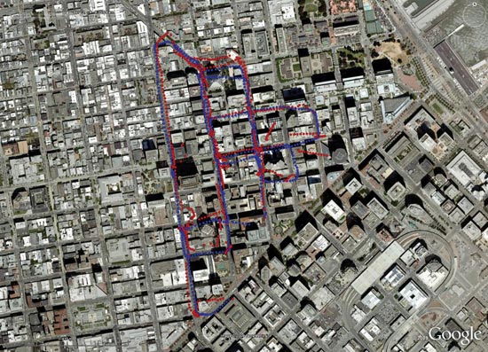
FIGURE1. Conventional test drive (two receivers)
Conventional Testing Methods
Traditionally, the simplest way to test the real-world performance of a GNSS receiver is to put it in a vehicle or a portable pack; drive or walk around an area of interest (typically a challenging environment such as an “urban canyon”); record position data; plot the trajectory on a map; and evaluate it visually. An example of this is shown in Figure 1 for two receivers, in this case driven through the difficult radio environment of downtown San Francisco.
While appealing in its simplicity and direct visual representation of the test drive, this approach does not allow for any quantitative assessment of receiver performance; judging which receiver is “better” is inherently subjective here. Different receivers often have different strong and weak points in their tracking and navigation algorithms, so it can be difficult to assess overall performance, especially over the course of a long trial. Also, an accurate evaluation of a trial generally requires some first-hand knowledge of the test area; unless local maps are available in sufficiently high resolution, it may be difficult to tell, for example, how accurate a trajectory along a wooded area might be.
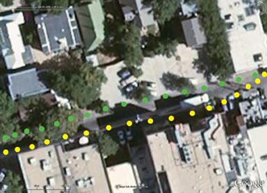
In Figure 2, it appears clear enough that the test vehicle passed down a narrow lane between two sets of buildings during this trial, but it can be difficult to tell how accurate this result actually is. As will be demonstrated below, making sense of a situation like this is essentially beyond the scope of the simple “visual plotting” test method.
FIGURE 2. Test result requiring local knowledge to interpret correctly.
To address these shortcomings, the simple test method can be refined through the introduction of a GNSS/INS truth reference system. This instrument combines the absolute position obtainable from GNSS with accurate relative measurements from a suite of inertial sensors (accelerometers, gyroscopes, and occasionally magnetometers) when GNSS signals are degraded or unavailable. The reference system is carried or driven along with the devices under test (DUTs), and produces a truth trajectory against which the performance of the DUTs is compared.
This refined approach is a significant improvement over the first method in two ways: it provides a set of absolute reference positions against which the output of the DUTs can be compared, and it enables a quantitative measurement of position accuracy. Examples of these two improvements are shown in Figure 3 and Figure 4.
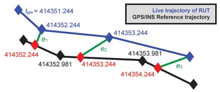
FIGURE 3. Improved test with GPS/INS truth reference: yellow dots denote receiver under test; green dots show the reference trajectory of GPS/INS.FIGURE 4. Time-aligned 2D error.
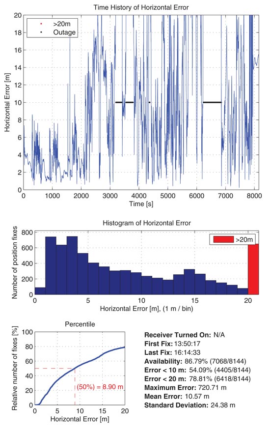
As shown in Figure 4, interpolating the truth trajectory and using the resulting time-aligned points to calculate instantaneous position errors yields a collection of scalar measurements en. From these values, it is straightforward to compute basic statistics like mean, 95th percentile, and maximum errors over the course of the trial. An example of this is shown in Figure 5, with the data (horizontal 2D error in this case) presented in several different ways. Note that the time interpolation step is not necessarily negligible: not all devices align their outputs to whole second boundaries of GPS time, so assuming a typical 1 Hz update rate, the timing skew between a DUT and the truth reference can be as large as 0.5 seconds. At typical motorway speeds, say 100 km/hr, this results in a 13.9 meter error between two points that ostensibly represent the same position. On the other hand, high-end GPS/INS systems can produce outputs at 100 Hz or higher, in which case this effect may be safely neglected.
FIGURE 5. Quantifying error using a truth reference
Despite their utility, both methods described above suffer from two fundamental limitations: results are inherently obtainable only in real time, and the scope of test coverage is limited to the number of receivers that can be fixed on the test rig simultaneously. Thus a test car outfitted with five receivers (a reasonable number, practically speaking) would be able to generate at most five quasi-independent results per outing.
Software Approach
The architecture of a software GNSS receiver is ideally suited to overcoming the limitations described above, as follows.
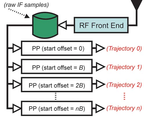
The raw IF data stream from the analog-to-digital converter is recorded to a file during the initial data collection. This file captures the essential characteristics of the RF chain (antenna pattern, downconverter, filters, and so on), as well as the signal environment in which the recording was made (fading, multipath, and so on). The IF file is then reprocessed offline multiple times in the lab, applying the results of careful profiling of various hardware platforms (for example, Pentium-class PC, ARM9-based embedded device, and so on) to properly model the constraints of the desired target platform. Each processing pass produces a position trajectory nominally identical to what the DUT would have gathered when running live. The complete multiple offset post-processi
ng (MOPP) setup is illustrated in Figure 6.
FIGURE 6. Multiple Offset Post-Processing (MOPP).
The fundamental improvement relative to a conventional testing approach lies in the multiple reprocessing runs. For each one, the raw data is processed starting from a small, progressively increasing time offset relative to the start of the IF file. A typical case would be 256 runs, with the offsets uniformly distributed between 0 and 100 milliseconds — but the number of runs is limited only by the available computing resources, and the granularity of the offsets is limited only by the sampling rate used for the original recording. The resulting set of trajectories is essentially the physical equivalent of having taken a large number of identical receivers (256 in this example), connecting them via a large signal splitter to a single common antenna, starting them all at approximately the same time (but not with perfect synchronization), and traversing the test route.
This approach produces several tangible benefits.
The large number of runs dramatically increases the statistical significance of the quantitative results (mean accuracy, 95th percentile error, worst-case error, and so on) produced by the test.
The process significantly increases the likelihood of identifying uncommon (but non-negligible) corner cases that could only be reliably found by far more testing using ordinary methods.
The approach is deterministic and completely repeatable, which is simply a consequence of the nature of software post-processing. Thus if a tuning improvement is made to the navigation filter in response to a particular observed artifact, for example, the effects of that change can be verified directly.
The proposed approach allows the evaluation of error models (for example, process noise parameters in a Kalman filter), so estimated measurement error can be compared against actual error when an accurate truth reference trajectory (such as that produced by the aforementioned GPS/INS) is available. Of course, this could be done with conventional testing as well, but the replay allows the same environment to be evaluated multiple times, so filter tuning is based on a large population of data rather than a single-shot test drive.
Start modes and assistance information may be controlled independently from the raw recorded data. So, for example, push-to-fix or A-GNSS performance can be tested with the same granularity as continuous navigation performance.
From an implementation standpoint, the proposed approach is attractive because it requires limited infrastructure and lends itself naturally to automated implementation. Setting up handful of generic PCs is far simpler and less expensive than configuring several hundred identical receivers (indeed, space requirements and RF signal splitting considerations alone make it impractical to set up a test rig with anywhere near the number of receivers mentioned above). As a result, the software replay setup effectively increases the testing coverage by several orders of magnitude in practice. Also, since post-processing can be done significantly faster than real time on modern hardware, these benefits can be obtained in a very time-efficient manner.
As with any testing method, the software approach has a few drawbacks in addition to the benefits described above. These issues must be addressed to ensure that results based on post-processing are valid and meaningful.
Error and Independence
The MOPP approach raises at least two obvious questions that merit further discussion.
How accurately does file replay match live operation?
Are runs from successive offsets truly independent?
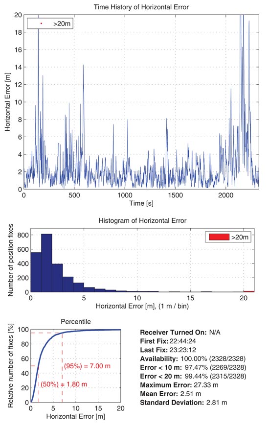
The first question is answered quantitatively, as follows. A general-purpose software receiver (running on an x86-class netbook computer) was driven around a moderately challenging urban environment and used to gather live position data (NMEA) and raw digital data (IF samples) simultaneously. The IF file was post-processed with zero offset using the same receiver executable, incorporating the appropriate system profiling to accurately model the constraints of real-time processing as described above, to yield a second NMEA trajectory. Finally, the two NMEA files were compared using the methods shown in Figure 4 and Figure 5, this time substituting the post-processed trajectory for the GPS/INS reference data. A plot of the resulting horizontal error is shown in Figure 7.
FIGURE 7. Quantifying error introduced by post-processing.
The mean horizontal error introduced by the post-processing approach relative to the live trajectory is on the order of 2.5 meters. This value represents the best accuracy achievable by file replay process for this environment.
More challenging environments will likely have larger minimum error bounds, but that aspect has not yet been investigated fully; it will be considered in future work. Also, a single favorable comparison of live recording against a single replay, as shown above, does not prove that the replay procedure will always recreate a live test drive with complete accuracy. Nevertheless, this result increases the confidence that a replayed trajectory is a reasonable representation of a test drive, and that the errors in the procedure are in line with the differences that can be expected between two identical receivers being tested at the same time.
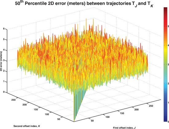
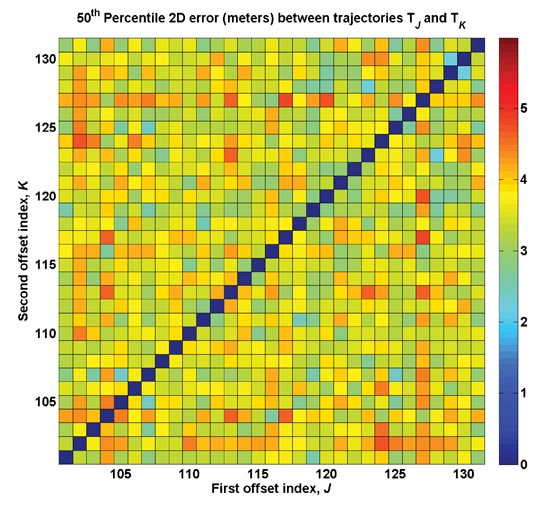
To address the question of run-to-run independence, consider two trajectories generated by post-processing a single IF file with offsets jB and kB, where B is some minimum increment size (one sample, one buffer, and so on), and define FJK to be some quantitative measurement of interest, for example mean or 95th percentile horizontal error. The deterministic nature of the file replay process guarantees FJK = 0 for j = k. Where j and k differ by a sufficient amount to generate independent trajectories, FJK will not be constant, but should be centered about some non-negative underlying value that represents the typical level of error (disagreement) between nominally identical receivers. As mentioned earlier, this is the approximate equivalent of connecting two matched receivers to a common antenna, starting them at approximately the same time, and driving them along the test trajectory.
Given these definitions, independence is indicated by an abrupt transition in FJK between identical runs ( j = k) and immediately adjacent runs (|j – k| = 1) for a given offset spacing B. Conversely, a gradual transition indicates temporal correlation, and could be used to determine the minimum offset size required to ensure run-to-run independence if necessary. As shown in Figure 8, the MOPP parameters used in this study (256 offsets, uniformly spaced on [0, 100 msec] for each IF file) result in independent outputs, as desired.
FIGURE 8. Verifying independence of adjacent offsets (upper: full view; lower: zoomed top view)
One subtlety pertaining to the independence analysis deserves mention here in the context of the MOPP method. Intuitively, it might appear that the offset size B should have a lower usable bound, below which temporal correlation begins to appear between adjacent post-processing runs. Although a detailed explanation is outside the scope of this paper, it can be shown that certain architectural choices in the design of a receiver’s baseband can lead to somewhat counterintuitive results in this regard.
As a simple example, consider a receiver that does not forcibly align its channel measurements to whole-second boundaries of system time. Such a device will produce its measurements at slightly different times with respect to the various timing markers in the incoming signal (epoch, subframe, and frame boundaries) for each different post-processing offset. As a result, the position solution at a given time point will differ slightly between adjacent post-processing runs until the offset size becomes smaller than the receiver’s granularity limit (one packet, one sample, and so on), at which point the outputs from successive offsets will become identical. Conversely, altering the starting point by even a single offset will result in a run sufficiently different from its predecessor to warrant its inclusion in a statistical population.
Application-to-Receiver Optimization
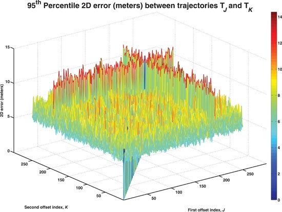
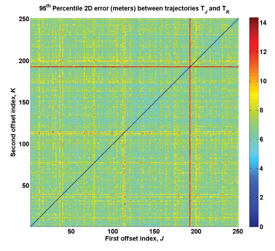
Once the independence and lower bound on observable error have been established for a particular set of post-processing parameters, the MOPP method becomes a powerful tool for finding unexpected corner cases in the receiver implementation under test. An example of this is shown in Figure 9, using the 95th percentile horizontal error as the statistical quantity of interest.
FIGURE 9. Identifying a rare corner case (upper: full view; lower: top view)
For this IF file, the “baseline” level for the 95th percentile horizontal error is approximately 6.7 meters. The trajectory generated by offset 192, however, exhibits a 95th percentile horizontal error with respect to all other trajectories of approximately 12.9 meters, or nearly twice as large as the rest of the data set. Clearly, this is a significant, but evidently rare, corner case — one that would have required a substantial amount of drive testing (and a bit of luck) to discover by conventional methods.
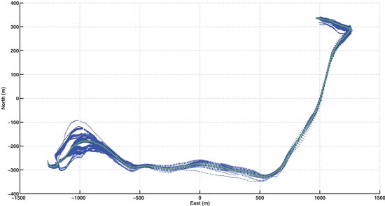
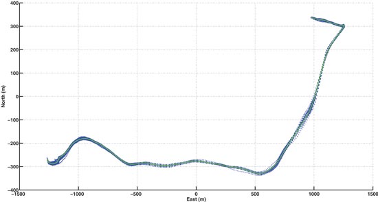
When an artifact of the type shown above is identified, the deterministic nature of software post-processing makes it straightforward to identify the particular conditions in the input signal that trigger the anomalous behavior. The receiver’s diagnostic outputs can be observed at the exact instant when the navigation solution begins to diverge from the truth trajectory, and any affected algorithms can be tuned or corrected as appropriate. The potential benefits of this process are demonstrated in Figure 10.
FIGURE 10. Before (top) and after (bottom) MOPP-guided tuning (blue = 256 trajectories; green = truth)
Limitations
While the foregoing results demonstrate the utility of the MOPP approach, this method naturally has several limitations as well. First, the IF replay process is not perfect, so a small amount of error is introduced with respect to the true underlying trajectory as a result of the post-processing itself. Provided this error is small compared to those caused by any corner cases of interest, it does not significantly affect the usefulness of the analysis — but it must be kept in mind.
Second, the accuracy of the replay (and therefore the detection threshold for anomalous artifacts) may depend on the RF environment and on the hardware profiling used during post-processing; ideally, this threshold would be constant regardless of the environment and post-processing settings.
Third, the replay process operates on a single IF file, so it effectively presents the same clock and front-end noise profile to all replay trajectories. In a real-world test including a large number of nominally identical receivers, these two noise sources would be independent, though with similar statistical characteristics. As with the imperfections in the replay process, this limitation should be negligible provided the errors due to any corner cases of interest are relatively large.
Conclusions and Future Work
The multiple offset post-processing method leverages the unique features of software GNSS receivers to greatly improve the coverage and statistical validity of receiver testing compared to traditional, hardware-based testing setups, in some cases by an order of magnitude or more. The MOPP approach introduces minimal additional error into the testing process and produces results whose statistical independence is easily verifiable. When corner cases are found, the results can be used as a targeted tuning and debugging guide, making it possible to optimize receiver performance quickly and efficiently.
Although these results primarily concern continuous navigation, the MOPP method is equally well-suited to tuning and testing a receiver’s baseband, as well its tracking and acquisition performance. In particular, reliably short time-to-first-fix is often a key figure of merit in receiver designs, and several specifications require acquisition performance to be demonstrated within a prescribed confidence bound. Achieving the desired confidence level in difficult environments may require a very large number of starts — the statistical method described in the 3GPP 34.171 specification, for example, can require as many as 2765 start attempts before a pass or fail can be issued — so being able to evaluate a receiver’s acquisition performance quickly during development and testing, while still maintaining sufficient confidence in the results, is extremely valuable.
Future improvements to the MOPP method may include a careful study of the baseline detection threshold as a function of the testing environment (open sky, deep urban canyon, and so on). Another potentially fruitful line of investigation may be to simulate the effects of physically distinct front ends by adding independent, identically distributed swaths of noise to copies of the raw IF file prior to executing the multiple offset runs.
Alexander Mitelman is GNSS research manager at Cambridge Silicon Radio. He earned his M.S. and Ph.D. degrees in electrical engineering from Stanford University. His research interests include signal quality monitoring and the development of algorithms and testing methodologies for GNSS.
Jakob Almqvist is an M.Sc. student at Luleå University of Technology in Sweden, majoring in space engineering, and currently working as a software engineer at Cambridge Silicon Radio.
Robin Håkanson is a software engineer at Cambridge Silicon Radio. His interests include the design of optimized GNSS software algorithms, particularly targeting low-end systems.
David Karlsson leads GNSS test activities for Cambridge Silicon Radio. He earned his M.S. in computer science and engineering from Linköping University, Sweden. His current focus is on test automation development for embedded software and hardware GNSS receivers.
Fredrik Lindström is a software engineer at Cambridge Silicon Radio. His primary interest is general GNSS software development.
Thomas Renström is a software engineer at Cambridge Silicon Radio. His primary interests include developing acquisition and tracking algorithms for GNSS software receivers.
Christian Ståhlberg is a senior software engineer at Cambridge Silicon Radio. He holds an M.Sc. in computer science from Luleå University of Technology. His research interests include the development of advanced algorithms for GNSS signal processing and their mapping to computer architecture.
James Tidd is a senior navigation engineer at Cambridge Silicon Radio. He earned his M.Eng. from Loughborough University in systems engineering. His research interests
include integrated navigation, encompassing GNSS, low-cost sensors, and signals of opportunity.
By Marcel Baracchi-Frei,
Grégoire Waelchli, Cyril Botteron,
and Pierre-André Farine
The idea of a software receiver is to replace the data processing implemented in hardware with software and to sample the analog input signal as close as possible to the antenna. Thus, the hardware is reduced to the minimum — antenna and analog-to-digital converters (ADCs) — while all the signal processing is done in software. As current mobile devices (such as personal digital assistants and smartphones) include more and more computing power and system features, it becomes possible to integrate a complete GNSS receiver with very few external components.
One advantage of a software receiver clearly lies in the low-cost opportunity, as the system resources such as the calculation power and system memory can be shared. Another advantage resides in the flexibility for adapting to new signals and frequencies. Indeed, an update can easily be performed by changing some parameters and algorithms in software, while it would require a new redevelopment for a standard hardware receiver.
Updating capabilities may become even more important in the future, as the world of satellite navigation is in complete effervescence: Europe is developing its own solution, Galileo, foreseen to be operational in 2013; China has undertaken a fundamental redevelopment of its current Compass navigation system; Russia is investing huge sums of money in GLONASS to bring it back to full operation; and the U.S. GPS system will see some fundamental improvements during the next few years, with new frequencies and new modulation techniques. At the same time, augmentation systems (either space-based or land-based) will develop all over the world.
These future developments will increase the number of accessible satellites available to every user — with the advantage of better coverage and higher accuracy. However, to take full advantage of the new satellite constellations and signals, new GNSS receivers and algorithms must be developed.
Definition and Types
The definition of a software receiver (SR) always brings some confusion among researchers and engineers in the field of communications and GNSS. For example, a receiver containing multiple hardware parts which can be reconfigured by setting a software flag or hardware pins of a chipset are regarded by some communication engineers to be a SR. In this article, however, we will consider the widely accepted SR definition in the field of GNSS; that is, a receiver in which all the baseband signal processing is performed in software by a programmable microprocessor.
Nowadays, software receivers can be grouped in three main categories:
field programmable gate arrays (FPGAs), which are sometimes also referred to the domain of SR. These receivers can be reconfigured in the field by software.
post-processing receivers include, among others, countless software tools or lines of code for testing new algorithms and for analyzing the GNSS signal, for example, to investigate GPS satellite failure or to decrypt unpublished codes.
real-time-capable software receivers group that will be further considered here.
A modern GNSS receiver normally contains a RF front-end, a signal acquisition, a tracking, and a navigation block. A hardware-based receiver accomplishes the residual carrier removal, PRN code-despreading, and integration at the system sampling rate. Until the late 1990s, due to the limited processing power of microprocessors, these signal functions could only be practically implemented in hardware.
The GNSS SR boom really started with the development of real-time processing capability. This was first accomplished on a digital signal processor (DSP) and later on a commercial conventional personal computer (PC). Today, DSPs are increasingly replaced by specialized processors for embedded applications.
Challenges
Data rate. The ideal software receiver would place the ADC as close as possible to the antenna to reduce hardware parts to a minimum. In that sense, the most straightforward approach consists of digitizing the data directly at the antenna, without pre-filtering or pre-processing. But as the Nyquist theorem must be fulfilled (that is, sampling with at least twice the highest signal frequency), this translates into a data rate that is, for the time being, too high to be processed by a microcontroller.
Considering the GPS L1 signal and assuming 1 quantization bit per sample, this leads to the following values:
In order to reduce the data throughput, a solution such as a low intermediate frequency (IF) or a sub-sampling analog front-end must be chosen. In a low IF front-end, the incoming signal is down-converted to a lower intermediate frequency of several megahertz. This allows working with a sampling (and data) rate that can be more easily handled by a microcontroller. With the new BOC signal modulations (used for the Galileo E1 and the modernized GPS L1 signals) that have no energy at and near DC, a zero-IF or homodyne architecture is also possible without SNR degredation due to DC offset, flicker noise, or even-order distortions.
The sub-sampling technique exploits the fact that the effective signal bandwidth in a GNSS signal is much lower than the carrier frequency. Therefore, not the carrier frequency but the signal bandwidth must be respected by the Nyquist theorem (assuming appropriate band-pass filtering). In this case, the modulated signal is under-sampled to achieve frequency translation via intentional aliasing. Again, if the GPS L1 signal is taken as an example with assuming 1 quantization bit per sample, this leads to the following values:
However, as the sub-sampling approach is still difficult to implement due to current hardware and resources limitations, a more classical solution based on an analog IF down-conversion is often chosen. That means that the signal is first down-converted to an intermediate frequency and afterwards digitized.
Baseband Processing. Considering an IF-based architecture, the ADC provides a data stream (real or complex), which is first shifted into baseband by at least one complex mixer. The signal is then multiplied with several code replicas (generally early, prompt, and late) and finally accumulated. Figure 1 shows an example of a real data IF architecture.
FIGURE 1. Real IF architecture
In hardware receivers, the local code and carrier are generally generated in real-time by means of a numerically controlled oscillator (NCO) that performs the role of a digital waveform generator by incrementing an accumulator by a per-sample phase increment. The resulting value is then converted to the corresponding amplitude value to recreate the waveform at any desired phase offset. The frequency resolution is typically in the range of a few millihertz with a 32-bit accumulator, and a sampling frequency in the range of a few megahertz.
Assuming that a look-up table (LUT) address can be obtained with two logical operations (one shift and one mask), and the corresponding LUT value reads with 1 memory access — which is quite optimistic — the amount of operations needed to generate the complex waveforms per channel is given in Table 1.
Source: Marcel Baracchi-Frei, Grégoire Waelchli, Cyril Botteron, and Pierre-André Farine
The real-time carrier generation is computationally expensive and is consequently not suitable for a one-to-one software implementation. Earlier studies [Heckler, 2004] demonstrated that, assuming that an integer operation and a multiplication take one and 14 CPU cycles, respectively (for an Intel Pentium 4 processor), the baseband operations (without carrier and code generation or navigation solution) would require at least a 3 GHz Intel Pentium 4 processor with 100 percent CPU load. Therefore, under these conditions, real-time operations are not suitable for embedded processors. Therefore standard hardware receiver architectures cannot be translated directly into software, and consequently new strategies must be developed to lower the processing load.
Status
A major problem with the software architecture is the important computing resources required for baseband processing, especially for the accumulation process. As a straightforward transposition of traditional hardware-based architectures into software would lead to an amount of operations which is not suitable for today’s fastest computers, two main alternate strategies have been proposed in the literature: the first relies on single-instruction multiple-data (SIMD) operations, which provide the capability of processing vectors of data. Since they operate on multiple integer values at the same time, SIMD can produce significant gains in execution speed for repetitive tasks such as baseband processing. However, SIMD operations are tied to specific processors and therefore severely limit the portability of the code.
The second alternative consists in the bitwise parallel operations (sometimes also referred to as vector processing in the literature), which exploit the native bitwise representation of the signal. The data bits are stored in separate vectors, one sign and one or several magnitude vectors, on which bitwise parallel operations can be performed. The objective is to take advantage of the universality, high parallelism, and speed of the bitwise operations for which a single integer operation is translated into a few simple parallel logical relations. While SIMD operations use advanced and specific optimization schemes, the latter methodology exploits universal CPU instructions set. The drawback of the bitwise operations is the different representation of the values. To be able to perform integer operations, a time consuming conversion is needed.
Single-Instruction Multiple-Data
In 1995, Intel introduced the first instance of SIMD under the name of Multi Media Extension (MMX). The SIMD are mathematical instructions that operate on vectors of data and perform integer arithmetic on eight 8-bit, four 16-bit, or two 32-bit integers packed into a MMX register (see Figure 2).
FIGURE 2. Single-instruction single-data versus single-instruction multiple-data.
On average, the SIMD operations take more clock cycles to execute than a traditional x86 operation. Anyhow, since they operate on multiple integers at the same time, MMX code can produce significant gains in execution speed for appropriately structured algorithms. Later SIMD extensions (SSE, SSE2, and SSE3) added eight 128-bit registers to the x86 instruction set. Additionally, SSE operations include SIMD floating point operations, and expand the type of integer operations available to the programmer.
SIMD operations are well suited to parallelize the operations of the baseband processing (BBP) stage. In particular, they can be used to allow the PRN code mixing and the accumulation to be performed concurrently for all the code replicas. With the help of further optimizations such as instruction pipelining, more than 600 percent performance improvement with the SIMD operations compared to the standard integer operations can be observed [Heckler, 2006].For this reason, most of the software receivers with real-time processing capabilities use SIMD operations [Heckler; Pany 2003; Charkhandeh, 2006 ].
Bitwise Operations. Bitwise operation (or vector processing) was first introduced into the SR domain in 2002 [Ledvina]. The method exploits the bit representation of the incoming signal, where the data bits are stored in separate vectors on which bitwise parallel operations can be performed. Figure 3 shows a typical data storage scheme for vector processing.
Source: Marcel Baracchi-Frei, Grégoire Waelchli, Cyril Botteron, and Pierre-André Farine
The sign information is stored in the sign word while the remaining bit(s) representing the magnitude is (are) stored in the magn word(s). The objective is to take advantage of the high parallelism and speed of the bitwise operations for which a single integer addition or multiplication is translated into simple parallel logical operations. The carrier mixing stage is reduced to one or a few simple logical operations which can be performed concurrently on several bits. In the same way, the PRN code removal only affects the sign word.
In a U.S. patent by Ledvina and colleagues, the complete code and carrier removal process requires two operations for each code replica (early, prompt, and late). The complexity can be even further reduced by more than 30 percent by considering one single combination of early and late code replicas (typically early-minus-late). This way, the authors claim an improvement of a factor of 2 for the bitwise method compared to the standard integer operations.
The inherent drawback of this approach is the lack of flexibility: the complexity of the process becomes bit-depth dependent and the signal quantification cannot be easily changed (while performing BBP with integers allows the signal structure to change significantly without code modification).
To overcome this limitation, a combination of bitwise processing and distributed arithmetic can be used [described in Waelchli, 2009]. The power-consuming operations are performed with bitwise operations, and to be able to keep the flexibility of the calculations, standard integer operations are used after the code and carrier removal. The conversion between the two methods is performed with distributed arithmetic that offers an extremely efficient way to switch between the two representations.
Another important aspect in a software receiver is the code and carrier generation. As these tasks represent a huge processing load, new solutions must be developed in this domain.
Code Generation
The pseudorandom noise (PRN) codes transmitted by the satellites are deterministic sequences with noise-like properties that are typically generated with tapped linear feedback shift registers (for GPS L1 C/A) or saved in memory (for Galileo E1). But in order to save processing power, it is preferable for software applications to compute off-line the 32 codes and store them in memory.
One method stores the different PRN codes in their oversampled representation (the code are pre-generated) [Ledvina, 2002]. As the incoming signal code phase is random, the beginning of the first code chip is in general not aligned with the beginning of a word and may occur anywhere within it. To overcome this issue, either all the possible phases can be stored in memory, or the code can be shifted appropriately during the tracking. While the first approach increases the memory requirements, the second requires further data processing in function of the phase mismatch. Regarding the Doppler compensation, all the PRN codes in the table are assumed to have a zero Doppler shift. The code phase errors due to this hypothesis are eliminated by choosing a replica code from the table whose midpoint occurs at the desired midpoint time. The only other effect of the zero Doppler shift assumption is a small correlation power loss which is not more than 0.014 dB if the magnitude of the true Doppler shift is less than 10 kHz [Ledvina patent]. This approach is very popular in the SR domain and can be found in several solutions.
Carrier Generation
The generation of a local carrier frequency is necessary to perform the Doppler removal. The standard trigonometric functions or the Taylor decompositions for the sines and cosines computation are too heavy for a software implementation and are seldom considered.
However, several other techniques exist to reduce the computational load for the carrier generation: the values for the carrier can be pre-generated and then stored in lookup tables. As this would require several gigabytes of memory to store all the possible frequencies, the values are recorded on a coarse frequency grid with zero phases and at the RF front-end sampling frequency. The carrier will thus be available in a sampled version. The limited number of available carrier frequencies introduces a supplementary mismatch in the Doppler removal process. This error can be compensated with a simple phase rotation of the accumulation results. This method is very popular in the SR domain, and many solutions take advantage of it to avoid the power-hungry real-time carrier generation.
Based on the same principle as above, Normark (2004) proposed a method that pre-computes a set of carrier frequency candidates to be stored in memory. The grid spacing is selected so as to minimize the loss due to Doppler frequency offset. Furthermore, to provide phase alignement capabilities of the carriers, a set of initial phases is also provided for each possible Doppler frequency, as illustrated in Figure 4.
FIGURE 4. Set of carrier frequency candidates.
Contrarily to the Ledvina approach and thanks to the phase alignement capabilities, the number of sampling points must not obligatorily correspond to an entire acquisition period. Therefore, the length of the frequency candidate vectors can be chosen with respect to the available memory space and becomes quasi independent of the sampling frequency.
Another approach consists in removing concurrently the Doppler from all received satellite signals [Petovello, 2006]. The algorithm is implemented as a look-up table containing one single frequency, and the carrier removal is performed for all channels with the same frequency, but the frequency error results normally in an unacceptable loss. To overcome this problem, the integration interval is split into sub-intervals for which a partial accumulation is computed.
The result is rotated proportionally to the frequency mismatch in the same way as in the method described above. The algorithm can be applied recursively and with an appropriate selection of the sub-intervals, and the total attenuation factor can be limited to a reasonable value. The author claims an improvement of up to 30 percent compared to the standard look-up table method with respect to the total complexity for both Doppler removal and correlation stages. Regarding the computational complexity, the Doppler removal stage remains unchanged, with the difference that it is only performed once for all satellites. But the rotation needs to be done for each of the sub-intervals. However, this algorithm remains difficult to implement (number of samples varies in one or more full C/A code chip, and the data alignment is different than the sub-interval boundaries).
Available Receivers
Today, software receivers can be found at university and commercial levels. The development not only includes programming solution but also the realization of dedicated RF front-ends. As these RF front-ends are able to capture more and more frequencies with increasing bit-rates and band-widths, the PC-based software receivers require a comparably complex interface to transfer the digitized IF samples into the computer’s memory.
Two classes of PC-based GNSS SR front-end solutions can be found. The first one uses commercially available ADCs that are either connected directly to the PC (for example, via the PCI bus) or that are working as stand-alone devices. The ADC directly digitizes the received IF signal, which is taken from a pure analog front-end. This solution is often found at the university and research institute level, where a high amount of flexibility is required; for example, at the Department of Geomatics Engineering of the University of Calgary, Cornell University, and the University FAF Munich’s Institute of Geodesy and Navigation.
The second solution is based on front-ends that integrate an ADC plus a USB 2.0 interface. Currently, an impressive number of commercial and R&D front-ends are available for the GNSS market. NordNav (acquired by CSR) and Accord were among the first to provide USB-based solutions. Another interesting development comes from the University of Colorado, which in an OpenGPS forum published all details on the RF and USB sections. More companies announced and continue to announce front-ends that are not only capable of capturing a single frequency, but several different bands. To be able to deal with this increasing bandwidth, the USB port is very well suited for SR development, and its maximum theoretical transfer rate of 480 MBit/s allows realizing GPS/Galileo multi-frequency high bandwidth front-ends.
Embedded Market. As mentioned in the introduction, the embedded market will gain increasing importance during the next few years. A growing number of receivers are developed for this market, supporting different embedded platforms (for example, Intel XScale, ARM-based, and DSP-based). Several companies offer commercial software receivers for the embedded market, among others NordNav and SiRF (acquired by CSR), ALK Technologies Inc., and CellGuide.
Commercial PC-Based Receivers. The first commercial GPS/Galileo receiver for a PC platform was presented in 2001 by NordNav. This SR can be compared to a normal GPS receiver, although the CPU load of this solution is still quite impressive. Several other solutions have been presented more recently. One of the first (car) navigation solutions was presented by ALK Technologies under the name CoPilot. The CPU load was drastically reduced, and this solution works on a standard commercial personal computer. The client does not really see a difference compared to a solution that is based on a hardware receiver.
Research Activities. Use in teaching and training is one of the most valuable and obvious application for software GNSS receivers. Receivers, for which the source code is available, allow the observation and inspection of almost every signal data by the researcher.
Several textbooks have been published related to software GNSS receivers. The pioneer in this area is James Bao-yen Tsui, who in 2000 wrote the first book on software receivers, Fundamentals of Global Positioning System Receivers: A Software Approach (Wiley-Interscience, updated in 2004). Kai Borre and co-authors published in 2006 a book that comes with a complete (post-processing) software receiver written in Matlab: A Software-Defined GPS and Galileo Receiver: A Single-Frequency Approach (Birkhäuser Boston, 1st edition).
The European Union is financing development of receivers for Galileo. One project was the Galileo Receiver Analysis and Design Application (GRANADA) simulation tool. Running under Matlab, GRANADA is realized as a modular and configurable tool with a dual role: test-bench for integration and evaluation of receiver technologies, and SR as asset for GNSS application developers.
Other companies provide toolboxes (in Matlab or C) that allow testing of new algorithms in a working environment and inspecting almost all data signals; for example, Data Fusion Corporation and NavSys.
Outlook
Software receivers have found their place in the field of algorithm prototyping and testing. They also play a key role for certain special applications. What remains unclear today is if they will enter and drastically change the embedded market, or succeed as generic high-end receivers.
A software GNSS receiver offers advantages including design flexibility, faster adaptability, faster time-to-market, higher portability, and easy optimization at any algorithm stage. However, a major drawback persists in the slow throughput and the high CPU load.
Many different companies and universities have projects running that seek to optimize and develop new algorithms and methods for a software implementation. The developments not only consider the software levels, but also extend in the direction of using additional hardware that is already available on a standard PC; for example, using the high performance graphic processing unit (GPU) for calculating the local carrier [Petovello, 2008].
On the opposite end of the spectrum from the mass market, the following factors seem to ensure that, sooner or later, high-end software receivers will be available:
High bandwidth signals (GPS and Galileo) can already be transferred into the PC in real time and processed.
The processing power is increasing, allowing real-time processing with a limited amount of multi-correlators. The introduction of new multi-core processors will be advantageous for software receivers.
Post-processing is one of the most important benefits of a software receiver, as it enables a re-analysis of the signal several times with all possible processing options. Increasing hard disk capacity facilitates storage of several long data sequences.
Some signal-processing algorithms such as frequency-domain tracking or maximum-likelihood tracking are much easier to implement in software than in hardware, as they require complex operations at the signal level.
History
During the 1990s, a U.S. Department of Defense (DoD) project named Speakeasy was undertaken with the objective of showing and proving the concept of a programmable waveform, multiband, multimode radio [Lackey, 1995]. The Speakeasy project demonstrated the approach that underlies most software receivers: the analog to digital converter (ADC) is placed as near as possible to the antenna front-end, and all baseband functions that receive digitized intermediate frequency (IF) data input are processed in a programmable microprocessor using software techniques rather than hardware elements, such as correlators. The programmable implementation of all baseband functions offers a great flexibility that allows rapid changes and modifications. This property is an advantage in the fast-changing environment of GNSS receivers as new radio frequency (RF) bands, modulation types, bandwidths, and spreading/dispreading and baseband algorithms are regularly introduced.
In 1990, researchers at the NASA/Caltech Jet Propulsion Laboratory introduced a signal acquisition technique for code division multiple access (CDMA) systems that was based on the Fast Fourier Transform (FFT) [van Nee, 1991]. Since then, this method has been widely adopted in GNSS SR because of its simplicity and efficiency of processing load.
In 1996, researchers at Ohio University provided a direct digitization technique — called the bandpass sampling technique — that allowed the placing of ADCs closer to the RF portions of GNSS SRs. Until this time, the implemented SRs in university laboratories post-processed the data due to the lack of processing power mentioned earlier.
Finally, in 2001, researchers at Stanford University implemented a real-time processing-capable SR for the GPS L1 C/A signal [Akos, 2001].
However, the GNSS SR boom really started with the development of real-time processing capability. This was first accomplished on a digital signal processor (DSP) and later on a commercial conventional personal computer (PC). Today, the DSPs are increasingly replaced by specialized processors for embedded applications.
Marcel Baracchi-Frei received a physics-electronics degree from the University of Neuchâtel, Switzerland, and is working as a project leader and Ph.D. candidate in the Electronics and Signal Processing Laboratory at the Swiss Federal Institute of Technology (EPFL).
GRÉGOIRE WAELCHLI received his degree of physics-electronics from the University of Neuchâtel and is now at EPFL for a Ph.D. thesis in the field of GNSS software receivers.
CYRIL BOTTERON received a Ph.D. with specialization in wireless communications from the University of Calgary, Canada, and now leads the EPFL GNSS and UWB research subgroups.
PIERRE-ANDRÉ FARINE is professor and head of the Electronics and Signal Processing Laboratory at EPFL, and associate professor at the University of Neuchâtel.
By Glenn MacGougan, Peter Ludvig Normark, and Christian Stahlberg
Published: January 2005 GPS World
In this month’s Innovation, we look at a further evolution of the GNSS receiver which offers the promise of flexibility, adaptability, and cost-effectiveness.—Richard Langley
 The Trimble Catalyst software-defined GNSS receiver for Android phones and tablets has been updated to support GLONASS. The update demonstrates the advantages of software GNSS for delivering new functionality faster and easier, according to Trimble.