Tag: GPS benchmarks

  • Using the new interactive ‘GPS on Bench Marks’ map

    Using the new interactive ‘GPS on Bench Marks’ map

    The National Geodetic Survey (NGS) is now developing the 2022 transformation model. Once again, NGS requests the assistance of the surveying and mapping community. This column provides examples to explain the symbology and use of the new version of the GPS on Bench Marks program for developing the 2022 transformation tool.

    My last column discussed the results of the Beta hybrid Geoid18 model, and the differences between the Beta model and the official hybrid geoid model, Geoid12B. It provided examples to explain the symbology of the Beta Geoid18 Web Map. It was noted that NGS analysts rejected stations based on pre- and post-modeled residuals but many times there wasn’t enough redundant information available to ensure the station should be rejected or used in the creation of the hybrid geoid model. As I have mentioned before, users should be commended for their participation in the GPS on Bench Marks program. The Geoid18 model is still in “Beta” so, hopefully, users will continue their support by evaluating the Beta hybrid geoid model and reporting their issues to NGS. Saying that, NGS’ GPS on Bench Marks program is now in a different phase.

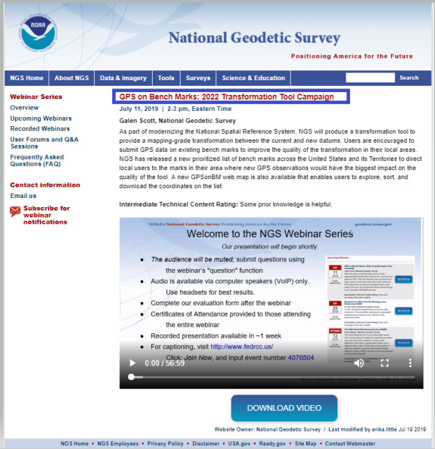
    NGS held a webinar in July on the latest GPS on Bench Marks program for developing the 2022 Transformation tool. The webinar was recorded and users can find the presentation here.  This was an excellent webinar and explained the functions of the web map. I would encourage readers to watch the webinar. It is an hour long but is worth while watching. See Figure 1 for information on the webinar.

    Figure 1: GPS on Bench Marks:2022 Transformation Tool Campaign Webinar. (Photo: National Geodetic Survey)
    Figure 1: GPS on Bench Marks:2022 Transformation Tool Campaign Webinar (Photo: National Geodetic Survey)

    As in the past, the NGS on Bench Marks program can be accessed from NGS’ web page (see Figure 2). The user clicks on the “GPS on Bench Marks” button to access the program’s web page.

    Figure 2: NGS Home Web Page (Photo: National Geodetic Survey)
    Figure 2: NGS Home Web Page (Photo: National Geodetic Survey)

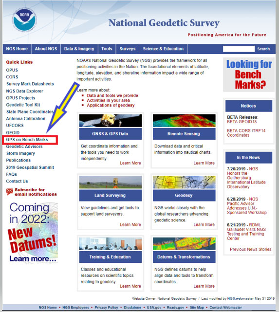
    Figure 3 depicts the home web page of the GPS on Bench Marks Program.

    Figure 3: GPS on Bench Marks Home Web Page (Photo: National Geodetic Survey)
    Figure 3: GPS on Bench Marks Home Web Page (Photo: National Geodetic Survey)

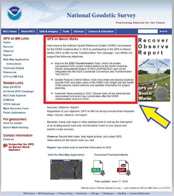
    The web page provides several reasons why users should continue to participate in the GPS on Bench Marks program. Figure 4 lists three reasons for helping NGS develop the 2022 Transformation Tool.

    Figure 4: Excerpt from GPS on Bench Marks Home Web Page

    GPS on Bench Marks

    Help improve the National Spatial Reference System (NSRS) and prepare for the NSRS modernization in 2022 by participating in the GPS on Bench Marks (GPS on BM) for the Transformation Tool campaign. Your efforts will support the following objectives:

    • Improve the 2022 Transformation Tool, >which will enable conversions from current vertical datums to the North American-Pacific Geopotential Datum of 2022 (NAPGD2022) and will be integrated into the NGS Coordinate Conversion and Transformation Tool (NCAT).

    • Update Passive Control Status: mark recoveries and shared solutions provide NGS and other users of the NSRS with insight into the health of the passive control network and updated information for project planning.

    • Automatic Reprocessing in 2022: Shared data will be automatically reprocessed and given new coordinates after the NSRS modernization occurs in 2022.

    I’d like to highlight a few of the benefits for participating in the GPS on Bench Marks program.

    (1) Improve the 2022 Transformation Tool, which will enable conversions from current vertical datums to the North American-Pacific Geopotential Datum of 2022 (NAPGD2022) and will be integrated into the NGS Coordinate Conversion and Transformation Tool (NCAT).

    > A goal of the transformation tool is to provide a model that will allow users to convert from the current North American Vertical Datum of 1988 (NAVD 88) to the new North American – Pacific Geopotential Datum of 2022 (NAPGD2022). The more bench marks that are occupied by GNSS and included in OPUS Shared solutions will enable NGS to generate a more detailed relationship between NAVD 88 and NAPGD2022. This will provide an accurate transformation tool in local areas which will facilitate the implementation of NAPGD2022 in surveying and mapping products and services.

    (2) Update Passive Control Status: mark recoveries and shared solutions provide NGS and other users of the NSRS with insight into the health of the passive control network and updated information for project planning.

    > An important part of the GPS on Bench Marks program is that it provides an indication of the status of the station. The last time a bench mark was leveled to varies greatly across the Nation. Many of stations in NGS’ Integrated Dataset haven’t been visited in over 50 years. The GPS on Bench Mark program can be useful to identify stations that have moved since the last time it was part of a leveling project. The mark recoveries will provide the latest status of a station which will help others in future project planning. More important, in my opinion, is that the OPUS shared solutions will identify stations that no longer have valid NAVD 88 published heights, and should be used with caution and flagged with a warning

    (3) Automatic Reprocessing in 2022: Shared data will be automatically reprocessed and given new coordinates after the NSRS modernization occurs in 2022.

    >> Any station that is part of the GPS on Bench Marks program and included in the OPUS Shared solution database will be given 2022 coordinates. This means that users will not have to resubmit their data to obtain the new coordinates in the new 2022 reference frames. This information will be useful during the implementation phase of the 2022 reference frames.

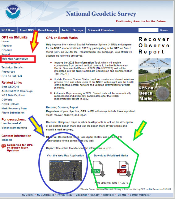
    As in the past, NGS is developing web-based products and services to facilitate users incorporating their data into the National Spatial Reference System (NSRS). They have developed a GPS on Bench Marks Web Map Application to inform users which stations they would like occupied by GNSS equipment. They realize that everyone is busy so they are trying to provide information, in near real time, on stations that have been occupied to reduce users occupying a station that already has two occupations. Figure 5 depicts the buttons that will connect the user to an interactive web map application. There are several ways the user can access the application: (1) click on the link titled “Web Map Application” – the red rectangle and arrow in the box titled “GPS on Bench Marks Web Map Application Site,” (2) click on the figure of the web based application – see the blue ellipse and blue arrow in the box, and (3) download the prioritized marks in XLS or Shape file format – see the green pentagon and green arrow in the box.

    Figure 5: GPS on Bench Marks Web Map Application Site (Photo: National Geodetic Survey)
    Figure 5: GPS on Bench Marks Web Map Application Site (Photo: National Geodetic Survey)

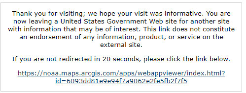
    Clicking on the Web Map Application button or picture will direct the user to a new website. It informs the user that they are leaving a U.S. Government Web Site for another site. See Figure 6. The user can either click on the statement or just wait until they are redirected the website. (See Figure 7.)

    Figure 6: Clicking on the Web Map Application Button or Picture (Photo: National Geodetic Survey)
    Figure 6: Clicking on the Web Map Application Button or Picture (Photo: National Geodetic Survey)
    Figure 7: GPS on Bench Marks For the Transformation Tool Interactive Web Map (Photo: National Geodetic Survey)
    Figure 7: GPS on Bench Marks For the Transformation Tool Interactive Web Map (Photo: National Geodetic Survey)

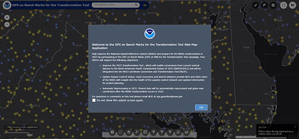
    Just click on the “OK” button to remove the splash screen. You can click the button “Do not show this splash screen again” so it doesn’t show up every time you access the web page. At the bottom of the web map is a legend that provides information about the map and allows the user to select various options. Figure 8 provides an example of legend buttons. The information box appears by clicking on a particular icon in the legend bar (the arrows indicate the icon and information box for that icon).

    Figure 8: Legend on GPS on Bench Marks Web Map Application Site (Photo: National Geodetic Survey)
    Figure 8: Legend on GPS on Bench Marks Web Map Application Site (Photo: National Geodetic Survey)

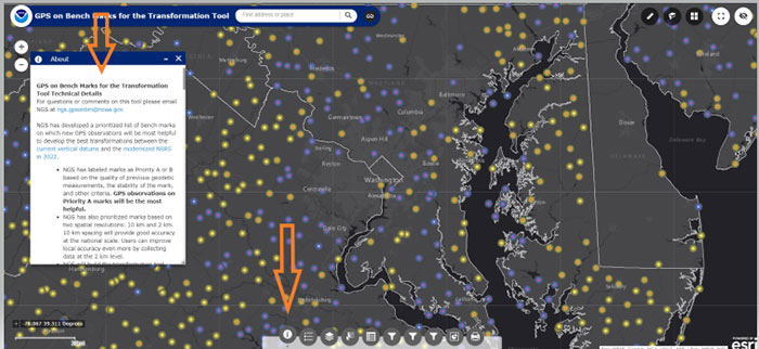
    There’s a lot of information provided in the information box. There’s a scroll bar on the right side of the box that provides the entire write up. Figure 9 provides several sections of the write up. I’ve highlighted sections in the write up to emphasis what NGS is trying to accomplish. NGS’ goal is to minimize the amount of work performed by users and maximize the amount of GNSS data provided to the development of the 2022 transformation tool.

    First, NGS has prioritized marks at two spatial resolutions: 10 km and 2 km. They want to reach a 10 km density to provide good national accuracy and a 2 km level to improve local accuracy. The Interactive Web Map allows users to zoom down to a level to identify individual stations selected by NGS. A 10-kilometer hexagonal lattice was developed to define the desired data density on the ground. For each hexagon, the goal was to identify a primary mark and a list of up to 4 secondary marks. The primary mark for each hexagon was added to the priority mark list. Secondary marks are listed and should be observed in cases where the primary mark cannot be found or is unobservable.

    To reduce duplication, when a single mark within a 10 km hexagon has two GPS observations that meet NGS requirements, that hexagon is marked as done and the station is removed from the prioritized list. This will help to reduce the number of surveyors occupying the same station over and over again, and increase the number of prioritized stations occupied with GNSS. After a 10-kilometer hexagon is marked as done, a group of up to thirteen 2 km hexagons is generated to define the opportunities to densify the model with additional marks.

    To assist in the selection of stations to be part of the GPS on Bench Marks program, NGS has prioritized stations as Priority A and B. Priority A being more important than priority B for the development of the 2022 transformation tool.

    Figure 9: Excerpts from GPS on Bench Marks for the Transformation Tool Technical Details

    For questions or comments on this tool please email NGS at [email protected].

    NGS has developed a prioritized list of bench marks on which new GPS observations will be most helpful to develop the best transformations between the current vertical datums and the modernized NSRS in 2022.

    • NGS has labeled marks as Priority A or B based on the quality of previous geodetic measurements, the stability of the mark, and other criteria. GPS observations on Priority A marks will be the most helpful.

    • NGS has also prioritized marks based on two spatial resolutions: 10 km and 2 km. 10 km spacing will provide good accuracy at the national scale. Users can improve local accuracy even more by collecting data at the 2 km level.

    • NGS will build the transformation tool with data submitted by December 31, 2021. The tool will interpolate over areas without GPSonBM data, meaning that the transformations will be less accurate in those areas.

    Priorities A and B

    Priority A
    Priority A marks meet the following specific criteria from their datasheets and are most likely to be used to create the transformation tools:
    • Vertical Order: FIRST, SECOND
    • Stability: A, B, C
    • Satellite: USEABLE
    • Last Recovery Condition: excluding “MARK NOT FOUND”

    Priority B
    Priority B marks are lower quality marks that will only be considered for use in the transformation tool to fill data gaps if no other data exists in the region.

    Spatial Resolution
    NGS has also prioritized marks at two spatial resolutions: 10 km and 2 km. NGS wants to reach a 10 km density to provide good national accuracy. Additionally, users can help improve local accuracy by collecting data at the 2 km level.

    To prioritize marks based on the two spatial resolutions, NGS created the following system:
    A 10-kilometer hexagonal lattice was developed to define the desired data density on the ground and help select appropriate marks within those areas throughout the U.S. and territories.
    • Hexagons with appropriate bench marks were identified.
    For each hexagon, a primary mark was selected and a list of up to 4 secondary marks — if available — were identified. The primary mark for each hexagon was added to the priority mark list. Secondary marks are listed and should be observed in cases where the primary mark cannot be found or is unobservable.
    To communicate when observations in a hexagon have been completed, the following process was developed:
    Once a single mark within a 10 km hexagon has two GPS observations that meet the requirements, that hexagon is marked as done and the observed mark is removed from the prioritized list.

    Once a 10 km hexagon is marked as done, a group of up to thirteen 2 km hexagons is generated to define the opportunities to densify the model with additional marks.
    In each of the 2 km hexagons, a primary mark is identified and a list of secondary marks is provided in case the primary mark cannot be found or is not observable. The new primary marks are added to the priority mark list. The number of 2 km hexagons will vary since not all areas have bench marks inside the 2 km lattice. See graphic below:

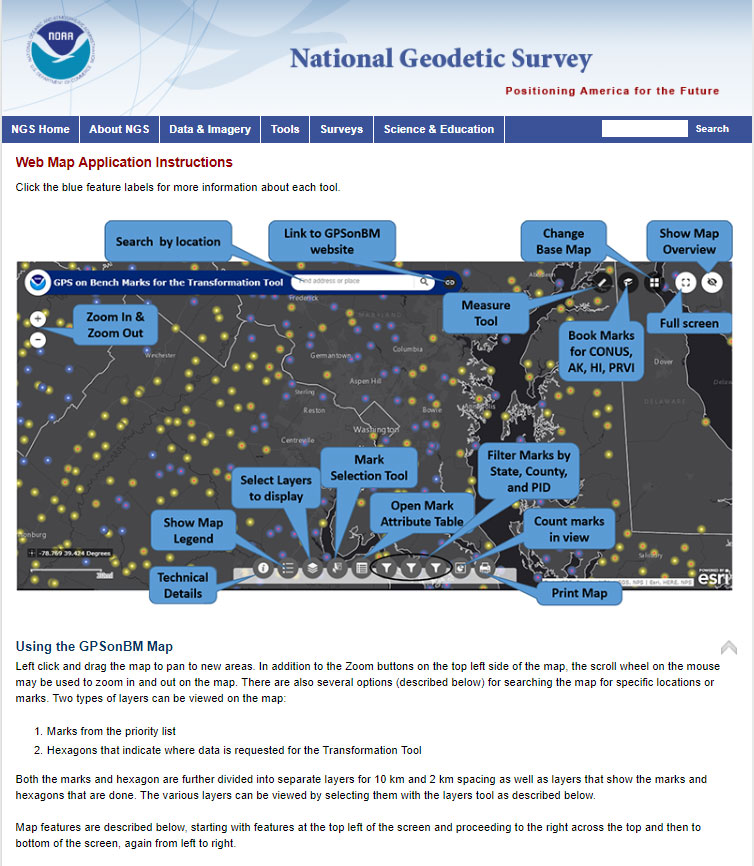
    Clicking on the Web Map Applications “Instructions” button will provide a summary of all of the tools available on the Web Map. See the arrow in Figure 10. The instruction page provides a lot of information and explains the function of each tool.

    Figure 10: GPS on Bench Marks Web Map Instructions Site (Photo: National Geodetic Survey)
    Figure 10: GPS on Bench Marks Web Map Instructions Site (Photo: National Geodetic Survey)

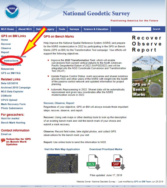
    Figure 11 provides an excerpt from that web page. All of the icons on the Web Map are explained on a mock up of a sample map in the beginning of the Instruction web page.

    Figure 11: GPS on Bench Marks Web Map Instructions List of Tools (Photo: National Geodetic Survey)
    Figure 11: GPS on Bench Marks Web Map Instructions List of Tools (Photo: National Geodetic Survey)

    The list of detailed descriptions of the tool is fairly long so I’ve provided some of the descriptions in Figure 12. The reader is referred to this page for the descriptions of all of the tools.

    Figure 12: Partial List of Descriptions of GPS on Bench Marks Web Map Instructions Tools

    Legend
    Clicking this button will display the legend for all of the active layers displayed on the map.

    Layer List
    Clicking this button will bring up the list of available layers to display on the map. By default, only the Priority List of marks at 10 km spacing appears. Users can select other layers to display on the map by clicking on the box to the left of the layer name. Once clicked, the box will show a check mark, and all layers with check marks are displayed on the map.


    Layer Descriptions:
    • Priority List 10 km – Marks requested for national coverage
    • Priority List 2 km – Marks requested to densify local areas
    • Priority List Done – All marks with enough observations to be considered for use in the Transformation Tool.
    • Hexagons 10 km – Areas where GPSonBM data is still requested to complete broad national coverage
    • Hexagons 10 km – Done – Areas where sufficient data exists
    • Hexagons 2 km -Areas where GPSonBM data may still be submitted to increase local accuracy of the transformation tool.
    • Hexagons 2 km – Done – Areas where sufficient data exists.

    Image: National Geodetic Survey
    Image: National Geodetic Survey

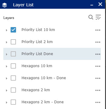
    Working with the Layer List
    Clicking on the ellipsis to the right of each layer opens a window with actions for that layer. Set visibility range allows the user to set the zoom level at which each layer appears. By default the visibility ranges are set to prevent too much data from being plotted at once which would slow down the application. Users with fast internet connections can change the visibility range to allow data to be displayed when zoomed out far enough to see the extents of larger states.

    Image: National Geodetic Survey
    Image: National Geodetic Survey

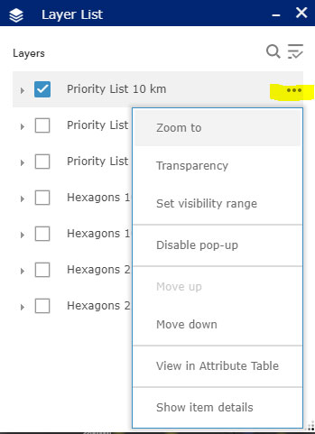
    Mark Selection Tool:

    This tool provides several options for selecting marks. First, change the layer to select from, click in the box to the left of the layer name. Click the green Select box and choose a selection method, then use the mouse to left-click on the map to draw the selection region. Selected marks’ icons will turn blue. Once marks are selected, click on the ellipsis to the right of the layer to open menu of actions that can be performed with selected marks. Using this menu, selected marks can be exported into csv, JSON, and GeoJSON formats.
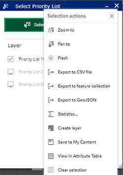
    Image: National Geodetic Survey
    Image: National Geodetic Survey

    Attribute Table
    This button opens a table at the bottom of the screen that displays all the information available on each mark.

    Image: National Geodetic Survey
    Image: National Geodetic Survey
    Image: National Geodetic Survey
    Image: National Geodetic Survey

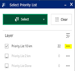
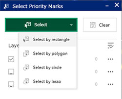
    Filters

    By State, County, and PID: This tool allows the user to filter the marks on the map down to specific states, counties, or PIDS. After selecting the filter option, click on the switch at the top right of the filter box and the map will pan and zoom to the selected area. If the marks do not appear on the map, try zooming in until they appear.

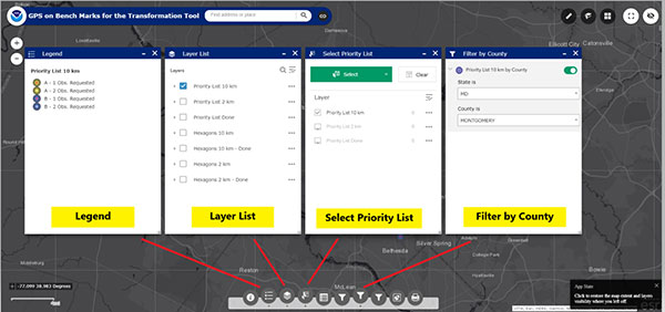
    Figure 13 provides four different options of the icons on the bottom of the web map. They include the “Legend,” Layer List,” Select Priority List,” and Filter by State. These options help the user focus on a particular area of interest. I would encourage the user to familiar themselves with each of these options because they help will make it easier to navigate the map and identify priority stations.

    Figure 13: Example of Several Options on the Legend on GPS on Bench Marks Web Map Application Site (Photo: National Geodetic Survey)
    Figure 13: Example of Several Options on the Legend on GPS on Bench Marks Web Map Application Site. Examples below are for the “Legend,” Layer List,” Select Priority List,” and Filter by County.” (Photo: National Geodetic Survey)

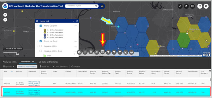
    Another important icon located at the bottom of the Web Map opens an attribute table of the bench marks. (See Figure 14). Once you open the Attribute table tool (see the red arrow in the box), a table of attributes of the stations appears at the bottom of the screen. If you click on a station in the table, the station gets highlighted on the map (see the blue arrow in the box). NGS’ Web Map Application makes it very easy to locate potential stations in a user’s area of interest.

    Figure 14: Example of the Attribute Table on the Legend on GPS on Bench Marks Web Map Application Site (Photo: National Geodetic Survey)
    Figure 14: Example of the Attribute Table on the Legend on GPS on Bench Marks Web Map Application Site (Photo: National Geodetic Survey)

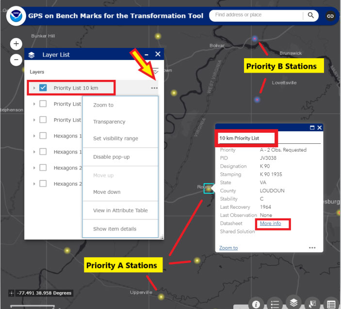
    When the user clicks on the Layer List tool, they can select which priority list they would like to see plotted on the map. They can click on the “More Info” button to obtain the latest NGS Datasheet. Figure 15 provides an example of A and B stations from the 10 km priority list in the Loudoun County, Virginia, region. The map highlights priority A and B stations; the user can than find more information about a specific station by clicking on the map.

    Figure 15: Excerpt from GPS on Bench Marks Web Map Layer List - Priority List 10 km (Photo: National Geodetic Survey)
    Figure 15: Excerpt from GPS on Bench Marks Web Map Layer List – Priority List 10 km (Photo: National Geodetic Survey)

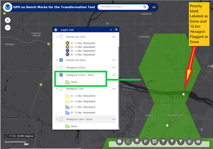
    A very interesting feature is that once a station is classified as done in a 10 km hexagon, the hexagon is colored green and flagged as done. There is no longer a requirement to occupy a station in that hexagon to assist the 2022 transformation tool for the National level of accuracy. See Figure 16 to see a 10-km hexagon labeled as “Done.” Note that the station considered “Done” is labeled with a white circle.

    Figure 16: An Example of a 10-km Hexagon in the Montgomery County, Maryland, and Loudoun County, Virginia, Region (Photo: National Geodetic Survey)
    Figure 16: An Example of a 10-km Hexagon in the Montgomery County, Maryland, and Loudoun County, Virginia, Region (Photo: National Geodetic Survey)

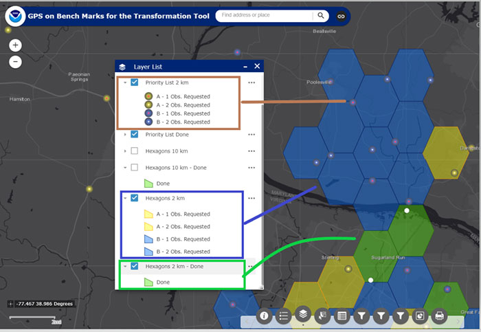
    Now the user can focus on the 2-km hexagon boxes to identify stations to improve the local accuracy of the 2022 transformation tool in their area of interest. Figure 17 provides an example of the 2-km hexagons with priority marks plotted within each 2-km hexagon. Once again, the symbology indicates A and B stations, and the 2-km hexagons that need more observations and the hexagons that are labeled as “Done.”

    Figure 17: An Example of 2-km Hexagons in the Montgomery County, Maryland, and Loudoun County, Virginia, Region (Photo: National Geodetic Survey)
    Figure 17: An Example of 2-km Hexagons in the Montgomery County, Maryland, and Loudoun County, Virginia, Region (Photo: National Geodetic Survey)

    NGS’ goal is to update the Interactive Web Map in “Near Real Time.” Of course, there’s always going to be some lag time from the time the user uploads their data into the OPUS Shared solution database to when the NGS 2022 Transformation Team reviews the data to ensure the results meet NGS’ criteria. Once again, NGS wants to minimize the amount of duplicate work performed by surveyors and maximize the number of stations contributing to the development of the 2022 transformation tool.

    This newsletter highlighted the next phase of NGS’ GPS on Bench Marks program; that is, the development of the 2022 transformation model. The newsletter provided examples to explain the symbology and use of the new version of the GPS on Bench Marks program. It provided web links to material explaining the new GPS on Bench Marks program such as NGS’ July 2019 webinar on the latest GPS on Bench Marks program for developing the 2022 Transformation tool. NGS has done a tremendous job of explaining the importance, process, and results of the GPS on Bench Marks Program. Several of my previous newsletters have highlighted the NGS GPS on Bench Marks program and how users have supported the development of the hybrid Geoid18 model: Hopefully, this support will continue to develop the best possible 2022 Transformation Tool.

  • A look at NGS’ GPS on benchmarks program in Alaska

    A look at NGS’ GPS on benchmarks program in Alaska

    The last column, February 2017, focused on addressing the following questions: (1) Is the large GPS on benchmarks residual due to an issue with the NAVD 88 orthometric height or the NAD 83 (2011) ellipsoid height? and (2) Should stations with large GPS on benchmarks residuals be included in the development of NGS’ hybrid geoid models? The column provided suggestions on how users can assist NGS in determining the reason for the large difference between the modeled hybrid geoid value and computed GNSS/leveling geoid computed value. It was mentioned that this information will be useful to NGS when developing hybrid geoid models and the 2022 Vertical Transformation model. My previous columns have focused on the conterminous United States. This column is going to discuss the GPS on benchmarks residuals for the state of Alaska.

    The February 2017 column noted that many of these large GPS on BM residuals could be due to an invalid NAVD 88 published height because the benchmark moved since the last time the height of the benchmark was adjusted and published, and/or an undetected error in an ellipsoid height due to a weak GNSS project design. The State of Alaska is very large; it has a sparse leveling network, and benchmarks are subject to movement due to ground conditions, isostatic effects, and seismic activity. The Geophysical Institute at the University of Alaska, Fairbank, has a lot of interesting reports on the movement in Alaska. Many of these stations would be identified as benchmarks with invalid heights when users follow Federal geodetic survey guidelines, procedures, and specifications. Benchmarks with invalid heights would not be used in controlling geodetic surveys and, in my opinion, should not be used in the hybrid geoid model. As I mentioned in my previous columns, this is not meant to be a criticism of NGS process for creating their hybrid geoid model. NGS’ goal is to create a hybrid geoid model that is consistent with published NAVD 88 values. I believe NGS is using all the data and information available to them. A goal of my last column was to emphasize to users the importance to strategically occupy stations to help support the GPS on benchmarks program which will result in the creation of a hybrid geoid model that accurately represents the current NAVD 88.

    First, let’s look at the leveling network design of Alaska. Figure 1 depicts the leveling network design used to establish heights in the NAVD 88. The figure indicates that most of the leveling data used in NAVD 88 was between 1965 and 1975. It should be noted that a major releveling project was performed in 1965 after the 1964 Good Friday Alaska Earthquake. There were some short leveling lines performed in the late 1980s and early 1991s. These data are now old and the question about whether the NAVD 88 height of the benchmark is still valid must be addressed.

    Figure 1 – Vertical Control used to establish heights in the NAVD 88 General Adjustment – It should be noted that nearly all of the leveling in the 1960s were performed after the 1964 earthquake (figure from a presentation titled “Achieving Great Heights: Toward a Better Vertical Reference System in Alaska” by Michael Dennis (National Geodetic Survey) and David B. Zilkoski (Geospatial Solutions by DBZ), March 28, 2014, 48th Annual Alaska Surveying and Mapping Conference, Fairbanks, Alaska)
    Figure 1 – Vertical Control used to establish heights in the NAVD 88 General Adjustment – It should be noted that nearly all of the leveling in the 1960s were performed after the 1964 earthquake (figure from a presentation titled “Achieving Great Heights: Toward a Better Vertical Reference System in Alaska” by Michael Dennis (National Geodetic Survey) and David B. Zilkoski (Geospatial Solutions by DBZ), March 28, 2014, 48th Annual Alaska Surveying and Mapping Conference, Fairbanks, Alaska)

    Alaska is prone to both episodic crustal motion (i.e. earthquakes) and the effects of long-term isostatic adjustment, which makes maintaining accurate vertical control difficult at best. (See figure 2 for a plot of earthquakes in Alaska). The 1964 Good Friday Alaska Earthquake, a magnitude of 9.2, changed heights as much as 8 feet. In addition to the initial damage at the time of the earthquake, there’s a post seismic vertical deformation movement that occurred. Suito and Freymueller (2009) provided a postseismic deformation model predictions for the 1964 earthquake [see box titled “Postseismic Velocity Predictions from Suito and Freymueller (2009)]”. An ArcGIS raster layer was developed using the grid values obtained from the website. Figure 3 is a plot of the vertical deformation model using Suito and Freymueller’s gridded dataset.

    Postseismic Velocity Predictions from Suito and Freymueller (2009)

    dbz-gps-newsletter-12-graph

    This page provides access to postseismic deformation model predictions for the 1964 earthquake. The model includes afterslip and viscoelastic relaxation (including the viscoelastic response to the afterslip), for the best-fit model derived by Suito and Freymueller (2009). That model includes a realistic slab geometry and a uniform asthenospheric relaxation time of 20 years. The full reference for the paper and the model is given below:
    Suito, H., and J. T. Freymueller, A viscoelastic and afterslip postseismic deformation model for the 1964 Alaska earthquake, J. Geophys. Res., doi:10.1029/ 2008JB005954, 2009.
    The model predictions are available in three different formats:

    1. A text file, Suito_vel.enu.txt with east, north and vertical model predictions evaluated on a 0.25 degree grid covering all of Alaska.
    2. A set of three netcdf grid files for use with GMT, for the east, north and vertical components. Interpolated values for any location can be generated easily with the GMT grdtrack program.
    o East component: Suito_east.grd.
    o North component: Suito_north.grd.
    o Vertical component: Suito_vert.grd.
    3. A MATLAB .mat file, visco_1964_SF2009.mat containing a structure with model velocity predictions at GPS sites in Alaska and the surrounding area.

    Units for all of these files are mm/yr.

    Figure 2 – Earthquakes in Alaska (https://pubs.er.usgs.gov/publication/ofr95624).
    Figure 2 – Earthquakes in Alaska.

    [INSERT FIGURE 3] Figure 3 – Post seismic Vertical Deformation Movement after the 1964 Alaska Earthquake (Suito, H., and J.T. Freymueller, “A viscoelastic and afterslip postseismic deformation model for the 1964 Alaska Earthquake, J. Geophy. Res,” ArcGIS raster layer was developed using grid values obtained from website: http://www.gps.alaska.edu/jeff/SF2009_postseismic.html)
    Figure 3 – Post seismic Vertical Deformation Movement after the 1964 Alaska Earthquake (Suito, H., and J.T. Freymueller, “A viscoelastic and afterslip postseismic deformation model for the 1964 Alaska Earthquake, J. Geophy. Res,” ArcGIS raster layer was developed using grid values obtained from this website.
    The NGS (formally the Coast and Geodetic Survey) releveled the area effected by the earthquake in 1965. Today, leveling is very expensive so estimating new heights of benchmarks after earthquakes really needs to be accomplished using GNSS surveys. However, as stated in my first column, June 2015, GNSS surveys provide accurate ellipsoid height when the appropriate procedures are followed, but an accurate geoid height is required to estimate an accurate GNSS-derived orthometric heights. Therefore, the question that needs to be addressed is how accurate is the geoid model in Alaska. As described in the last column, the GPS on benchmarks program is one method of evaluating the GNSS/Leveling/Geoid combined system.

    Saying that, Alaska’s system of NAVD88 benchmarks is based on old leveling data and, due to ground ice conditions and crustal movement, are subject to changes in heights. This makes it difficult to evaluate the geoid model in Alaska using published NAVD 88 heights. However, NGS’ GPS on benchmarks program can help to identify outliers and long wavelength trends between NAVD 88 heights and GNSS-derived orthometric heights. GPS on BMs residuals using the published GEOID12B values in the State of Alaska were generated using the data from the NGS’ website. I described these data and the process in my February 2017 column. Figures 4 through 6 depict the GPS on benchmarks residuals using the hybrid geoid model GEOID12B for stations in Alaska. It should be noted that only bench marks that had NAD 83 (2011) published coordinates and NAVD 88 published heights with the attribute of “Adjusted” were used in this analysis. This analysis does not include any OPUS results.

    Figure 4 – GPS on Bench Mark Residuals Using Geoid12B in the State of Alaska – {GPS on BMs Residual = [GEOID12B value – (NAD 83 (2011) ellipsoid height value – NAVD 88 orthometric height value)]}. The Residuals are Depicted by Symbols (units = cm)
    Figure 4 – GPS on Benchmark Residuals Using Geoid12B in the State of Alaska – {GPS on BMs Residual = [GEOID12B value – (NAD 83 (2011) ellipsoid height value – NAVD 88 orthometric height value)]}. The Residuals are Depicted by Symbols (units = cm)
    Figure 5 – GPS on Bench Mark Residuals Using Geoid12B in the State of Alaska –{GPS on BMs Residual = [GEOID12B value – (NAD 83 (2011) ellipsoid height value – NAVD 88 orthometric height value)]}. The Value of the Residuals are Labeled (units = cm)
    Figure 5 – GPS on Benchmark Residuals Using Geoid12B in the State of Alaska –{GPS on BMs Residual = [GEOID12B value – (NAD 83 (2011) ellipsoid height value – NAVD 88 orthometric height value)]}. The Value of the Residuals are Labeled (units = cm)
    Figure 6 – GPS on Bench Mark Residuals Using Geoid12B in the Haines and Skagway, Alaska, Region {GPS on BMs Residual = [GEOID12B value – (NAD 83 (2011) ellipsoid height value – NAVD 88 orthometric height value)]}. (units= cm)
    Figure 6 – GPS on Benchmark Residuals Using Geoid12B in the Haines and Skagway, Alaska, Region {GPS on BMs Residual = [GEOID12B value – (NAD 83 (2011) ellipsoid height value – NAVD 88 orthometric height value)]}. (units= cm)
    Looking at figures 4-6, most of the GPS on BMs residuals using GEOID12B appear to be less than a couple of centimeters. There are several stations that have large outliers but this is seen in every State in the conterminous United States. The small residuals using GEOID12B doesn’t really tell us much because the large threshold level used by the NGS Geoid Team can mask some issues. This was demonstrated in my last column. Notice that figure 6 only shows two GPS on BMs residuals in the Haines and Skagway area of Alaska. This is an area where more GPS on BMs would be helpful to evaluate the geoid model.

    As I’ve mentioned in my previous columns, the user should analyze the GPS on BMs stations using the latest experimental gravimetric geoid that includes the new airborne GRAV-D data, e.g. xGeoid16b. NGS has a website that enables users to compute geoid height values using the latest experimental gravimetric geoid model. All benchmarks in Alaska that had NAD 83 (2011) published coordinates were submitted as input to the NGS’ xGeoid16 website and the results were used to create a file of GPS on BMs residuals for the State of Alaska. An example of the output from the xGeoid16 website is provided in the box titled “Output from xGeoid16 Website.” NGS’ experimental geoid website was described in my October 2015 column.

    dbz-gps-newsletter-12-chart

    It should be noted that the input to the xGeoid16 website was NAD 83 (2011) coordinates and the output was provided in the IGS08 reference frame; therefore, the xGeoid16b geoid heights are referenced to IGS08. The GPS on BMs residuals was computed using the formula GPS on BMs Residual = [xGEOID16b value – (IGS08 ellipsoid height value – NAVD 88 orthometric height value)]. Figure 7 is a plot of the GPS on BMs residuals computed using xGeoid16b geoid values, IGS08 ellipsoid heights, and NAVD 88 orthometric heights.

    Figure 7 – GPS on Bench Mark Residuals Using xGeoid16b in the State of Alaska – Referenced to IGS08 (units = cm) – {GPS on BMs Residual = [xGEOID16b value – (IGS08 ellipsoid height value – NAVD 88 orthometric height value)]}. Green Line Represents the Leveling Lines
    Figure 7 – GPS on Benchmark Residuals Using xGeoid16b in the State of Alaska – Referenced to IGS08 (units = cm) – {GPS on BMs Residual = [xGEOID16b value – (IGS08 ellipsoid height value – NAVD 88 orthometric height value)]}. Green Line Represents the Leveling Lines
    Figure 7 indicates that there is an obvious bias of about a meter between the GNSS-derived orthometric heights referenced to IGS08 and the NAVD 88. This bias is expected since these GPS on BMs residuals are referenced with respect to IGS08. This has been described in more detail in my December 2016 column, and depicted in a figure on the NGS website. A bias and trend from the GPS on BMs residuals was removed by performing a least squares best fit planar surface of the differences (basically solving for a bias and a North-South and East-West tilt). Figure 8 is a plot of the GPS on BMs residuals using xGeoid16b in Alaska were a bias and trend was removed from the original computed GPS on BMs residuals that are depicted in figure 7. These GPS on BMs residuals will be used to identify outliers and will be referred to as GPS on BMs residuals (with a trend removed) in the reminder of this column.

    Figure 8 – GPS on Bench Mark Residuals Using xGeoid16b in the State of Alaska – Referenced to IGS08 with a trend removed– {GPS on BMs Residual = [xGEOID16b value – (IGS08 ellipsoid height value – NAVD 88 orthometric height value)]}. (units = cm) – Green Line Represents the Leveling Lines
    Figure 8 – GPS on Benchmark Residuals Using xGeoid16b in the State of Alaska – Referenced to IGS08 with a trend removed– {GPS on BMs Residual = [xGEOID16b value – (IGS08 ellipsoid height value – NAVD 88 orthometric height value)]}. (units = cm) – Green Line Represents the Leveling Lines
    The large absolute difference and tilt are not concerning, it’s the large relative differences between closely-spaced stations that need to be identified and explained. Removing the bias and trend in the GPS on BMs residuals is useful in identifying large relative differences between neighboring stations.

    Figure 9 is another plot of the GPS on BMs residuals using xGeoid16b with the trend removed using different symbology. The “up” blue arrows indicated a positive residual and a “down” red arrow indicates a negative residual. It’s not surprising to see both positive and negative residuals because a trend was removed from the residuals.

    Figure 9 – GPS on Bench Mark Residuals Using xGeoid16b in the State of Alaska - {GPS on BMs Residual = [xGEOID16b value – (IGS08 ellipsoid height value – NAVD 88 orthometric height value)]}. Referenced to IGS08 with a trend removed (units = cm) - “up” blue arrows indicated a positive residual and a “down” red arrow indicates a negative residual
    Figure 9 – GPS on Benchmark Residuals Using xGeoid16b in the State of Alaska – {GPS on BMs Residual = [xGEOID16b value – (IGS08 ellipsoid height value – NAVD 88 orthometric height value)]}. Referenced to IGS08 with a trend removed (units = cm) – “up” blue arrows indicated a positive residual and a “down” red arrow indicates a negative residual
    What should be noticed is that there are a lot of large negative and positive residuals. Figure 10 is a plot of the GPS on BMs residuals (with a trend removed) with residuals greater than +/- 20 cm labeled. It may be difficult to see in the plot but there are two residuals in the Hains and Skagway, Alaska, region (see right corner of figure 10). Both stations have large positive GPS on BMs residuals. What is important is that the relative difference between the two stations is also large, i.e., 42 cm (80.4 cm – 38.4 cm). We will address this difference later in this column.

    Figure 10 – GPS on Bench Mark Residuals Using xGeoid16b in the State of Alaska –– [GPS on BMs Residual = [xGEOID16b value – (IGS08 ellipsoid height value – NAVD 88 orthometric height value)]. Referenced to IGS08 with a trend removed (units = cm) – Residuals greater than 20 cm are labeled.
    Figure 10 – GPS on Benchmark Residuals Using xGeoid16b in the State of Alaska –– [GPS on BMs Residual = [xGEOID16b value – (IGS08 ellipsoid height value – NAVD 88 orthometric height value)]. Referenced to IGS08 with a trend removed (units = cm) – Residuals greater than 20 cm are labeled.
    As previously mentioned, investigating GPS on BMs with large relative differences between closely-spaced stations helps to identify outliers. Figure 11 is a plot of the GPS on BMs residual (with a trend removed) in the Matanuska-Susitna Borough, Alaska, region. There are several stations that are relatively close to each other (TT2213, TT2332, and TT2299) and have large relative GPS on BMs residuals. That is, the relative difference in GPS on BMs residuals between stations TT2313 and TT2332, 24 km apart, is -9.9 cm (-6.3 cm – 3.6 cm), and between stations TT2332 and TT2299, 19 km apart, the difference in GPS on BMs residual is -26.3 cm [-32.6 cm – (-6.3 cm)]. These stations have published NAVD 88 heights but should stations with large GPS on BM residuals be included in the development of NGS’ hybrid geoid models? At a minimum, other stations near these stations should be occupied with GNSS to help determine if other monuments in the area have moved in the similar manner.

    Figure 11 – GPS on Bench Mark Residuals Using xGeoid16b in the Matanuska-Susitna Borough, Alaska, Region – Large Difference between two relatively closely spaced stations (TT2313 and TT2332) - Referenced to IGS08 with a trend removed – {GPS on BMs Residual = [xGEOID16b value – (IGS08 ellipsoid height value – NAVD 88 orthometric height value)]}. (units = cm)
    Figure 11 – GPS on Benchmark Residuals Using xGeoid16b in the Matanuska-Susitna Borough, Alaska, Region – Large Difference between two relatively closely spaced stations (TT2313 and TT2332) – Referenced to IGS08 with a trend removed – {GPS on BMs Residual = [xGEOID16b value – (IGS08 ellipsoid height value – NAVD 88 orthometric height value)]}. (units = cm)
    Figure 2, a USGS plot of earthquakes in Alaska, highlighted the problems with maintaining reliable, accurate NAVD 88 orthometric heights in Alaska. Figure 12 is a plot of GPS on BMs residuals (with a trend removed) using xGeoid16b in the State of Alaska with an overlay of fault lines. The ArcGIS layer of fault lines was obtained from ArcGIS online layers. Looking at figure 12, it’s obvious that the heights of benchmarks in Alaska are probably being influenced by seismic activity. Figure 13 is a plot of the vertical velocity values at GNSS stations generated by UNAVCO’s GPS Velocity Viewer Program at this website.

    Figure 12 – GPS on Bench Mark Residuals Using xGeoid16b in the State of Alaska with an Overlay of Fault Lines – Residuals are referenced to IGS08 with a trend removed – {GPS on BMs Residual = [xGEOID16b value – (IGS08 ellipsoid height value – NAVD 88 orthometric height value)]}. (units = cm)
    Figure 12 – GPS on Benchmark Residuals Using xGeoid16b in the State of Alaska with an Overlay of Fault Lines – Residuals are referenced to IGS08 with a trend removed – {GPS on BMs Residual = [xGEOID16b value – (IGS08 ellipsoid height value – NAVD 88 orthometric height value)]}. (units = cm)
    Looking at figure 13, it is obvious that benchmarks that haven’t been releveled in the past 30 years could have been significantly influenced by crustal movement.

    Figure 13 – Vertical Velocity estimated at GNSS Station in Alaska using UNAVCO’s GPS Velocity-Viewer Program: Figure generated from the following website: http://www.unavco.org/software/visualization/GPS-Velocity-Viewer/GPS-Velocity-Viewer.html
    Figure 13 – Vertical Velocity estimated at GNSS Station in Alaska using UNAVCO’s GPS Velocity-Viewer Program: Figure generated from this website.

    Figure 14 is the same plot as figure 11 with an overlay of the fault lines. Are these stations being influenced by crustal motion? Repeat measurements are needed to address this issue. There is a great opportunity to assist in the development and assessment of hybrid geoid models if researchers and others that are conducting campaign GNSS surveys with long static occupations share their results with NGS. NGS has a Regional Geodetic Advisory in Alaska that could help facilitate getting the appropriate information to NGS’ geoid team. Nicole Kinsman is the NGS Regional Geodetic Advisor for Alaska. Ms. Kinsman is very knowledgeable on National Spatial Reference System (NSRS) issues in Alaska. She was very helpful to me as I was preparing this column.

    Figure 14 - GPS on Bench Mark Residuals Using xGeoid16b in the Matanuska-Susitna Borough, Alaska, Region with an overlay of Fault Lines – Large Difference between two relatively closely spaced stations (TT2313 and TT2332) - Referenced to IGS08 with a trend removed – {GPS on BMs Residual = [xGEOID16b value – (IGS08 ellipsoid height value – NAVD 88 orthometric height value)]}. (units = cm)
    Figure 14 – GPS on Benchmark Residuals Using xGeoid16b in the Matanuska-Susitna Borough, Alaska, Region with an overlay of Fault Lines – Large Difference between two relatively closely spaced stations (TT2313 and TT2332) – Referenced to IGS08 with a trend removed – {GPS on BMs Residual = [xGEOID16b value – (IGS08 ellipsoid height value – NAVD 88 orthometric height value)]}. (units = cm)
    Figure 15 is a plot of GPS on BMs residuals in the Yukon-Koyukuk borough, Alaska, region. Notice that there’s a large difference between relatively closely-spaced stations TT3571 and TT3555, 22.6 cm (31.7 cm – 9.1 cm). Saying that, the plot also depicts all the fault lines around these stations. This is another example of how difficult it is to maintain reliable orthometric heights in Alaska.

    Figure 15 – GPS on Bench Mark Residuals Using xGeoid16b in Yukon-Koyukuk Borough, Alaska, region with an Overlay of Fault Lines – Large Difference between two relatively closely spaced stations (TT3571 and TT3557) - Referenced to IGS08 with a trend removed – {GPS on BMs Residual = [xGEOID16b value – (IGS08 ellipsoid height value – NAVD 88 orthometric height value)]}. (units = cm)
    Figure 15 – GPS on Benchmark Residuals Using xGeoid16b in Yukon-Koyukuk Borough, Alaska, region with an Overlay of Fault Lines – Large Difference between two relatively closely spaced stations (TT3571 and TT3557) – Referenced to IGS08 with a trend removed – {GPS on BMs Residual = [xGEOID16b value – (IGS08 ellipsoid height value – NAVD 88 orthometric height value)]}. (units = cm)
    Figure 16 is a plot of GPS on BMs residuals in the Haines and Skagway, Alaska, region, with an overlay of fault lines. Figure 10 highlighted that the two stations, TT0118 and TT8080, have a large relative difference (42 cm) but figure 16 indicates that the two stations lie between a couple of fault lines.

    Figure 16 – GPS on Bench Mark Residuals Using xGeoid16b in the Skagway, Alaska, Region with an Overlay of Fault Lines - Referenced to IGS08 with a trend removed – {GPS on BMs Residual = [xGEOID16b value – (IGS08 ellipsoid height value – NAVD 88 orthometric height value)]}. (units = cm)
    Figure 16 – GPS on Benchmark Residuals Using xGeoid16b in the Skagway, Alaska, Region with an Overlay of Fault Lines – Referenced to IGS08 with a trend removed – {GPS on BMs Residual = [xGEOID16b value – (IGS08 ellipsoid height value – NAVD 88 orthometric height value)]}. (units = cm)
    What does this mean to surveyors and mappers in Alaska? In my opinion, the new 2022 Vertical Reference Datum, denoted as the North American-Pacific Geopotential Datum of 2022 (NAPGD 2022) will help Alaskans maintain a vertical reference frame that’s reliable and traceable. Saying that, it is extremely important to know the relative accuracy of the geoid model used to establish GNSS-derived orthometric heights in NAPGD2022. NGS is performing projects to evaluate the relative accuracy of the gravimetric geoid model. The projects are known as Geoid Slope Validation Surveys. I would encourage the Alaska surveying and mapping community to develop plans to transition to the new NAPGD2022. Evaluation of the experimental gravimetric geoid model is critical to the implementation of the new 2022 datum and should be part of a transition plan. Performing a geoid slope validation project similar to NGS may be too expensive to be performed by Alaskans. However, Alaskans may be able to perform low budget geoid slope evaluation surveys. These surveys could include performing combined GNSS and leveling surveys to evaluate the relative accuracy of the gravimetric geoid model in areas that require accurate orthometric heights. Performing several of the gravimetric geoid evaluation surveys in major cities and/or areas that require accurate heights would help to facilitate the implementation of NAPGD2022.

    These types of geoid evaluation surveys should also be performed in other areas of the country that are influenced by crustal movement. For example, the published NAVD 88 heights in southern Louisiana and other parts of the Gulf Coast of the United States are influenced by subsidence. NAPGD2022 will provide a more efficient and cost-effective way to maintain consistent orthometric heights. Once again, evaluating the relative accuracy of the gravimetric geoid model is critical to the implementation of NAPGD2022.