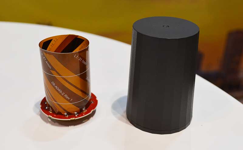
The new helical antenna in both housed (right) and unhoused form. (Photo: Allison Barwacz)
Tallysman, a manufacturer of high-performance GNSS and iridium antennas, launched the first three products of a new range of helical antennas. Additional models will be announced in the third quarter of 2019 and onward.
Tallysman exhibited at booth 3739 at AUVSI Xponential 2019, which took place April 29 to May 2 in Chicago.
The first three models of the Tallysman helical family are:
HC871 (25g) – A housed, dual band, active GNSS antenna, supporting GPS L1/L2,
GLONASS G1/G2, Galileo E1, and BeiDou B1.
HC872 (36g) – A housed, dual band, active GNSS antenna, supporting GPS L1/L2,
GLONASS G1/G2, Galileo E1, BeiDou B1, and L-Band services.
HC600 (18g) – A housed, passive Iridium antenna.
The active GNSS helical antennas feature a low-current, low-noise amplifier (LNA), and include integrated low-loss pre-filters, to protect against harmonic interference from high amplitude interfering signals, such as 700-MHz band LTE and other near in-band cellular signals.
Available in both housed and embedded OEM versions, the lightweight Tallysman helical antennas have excellent axial ratios, making them ideal for a variety of high-precision unmanned aerial vehicle (UAV) applications, the company said.
The housed Tallysman helical antenna models feature a robust, military-grade plastic case, while the embedded Tallysman helical antenna models can be custom-tuned for any application and configured with a variety of cables and connectors.
“We think — if anything — the price-performance ratio is the biggest benefit,” Allen Crawford, director of key accounts at Tallysman, told GPS World. “The pre-filter is also unique to us; the robustness of the enclosure is unique to us; and also the shortness, which is important to a lot of aerodynamic vehicles.”
Patents have been applied for with respect to several aspects of these new products.
“There is a clear requirement for lightweight, high performance antennas for the rapidly growing UAV market,” said Tallysman President and CTO Gyles Panther. “These new patented helical products are an extension to our existing range of superlight L1/L2 patch antennas, and will provide customers with a wider choice of antenna formats to suit their specific application requirements. These are the first of a number of new products we plan to introduce for this application to support our already wide customer base for UAV antennas.”
New developments in antenna technology empower the final positioning solution with better accuracy and reliability. Leading experts discuss the technology advances producing greater user benefits.
The increasing prevalence of both intentional and inadvertent jamming, new wider bandwidths, and the significance of antenna phase-center variation all bring changes to the dynamic and evolving antenna sector.
Javad Ashjaee (Photo: Javad GNSS)
Javad Ashjaee
President & CEO, JAVAD GNSS
Advanced filtering techniques enable our antennas to defend against jammers and spoofers and to inform users with the details of these intrusive actions when they are detected.
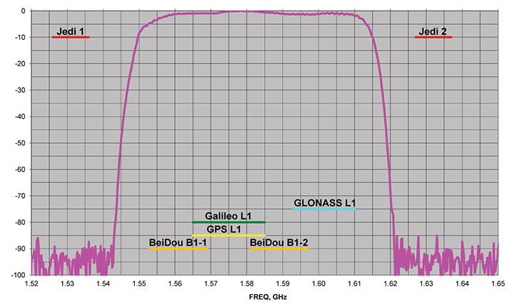
Near-Band Interference. The J-Shield is a robust filter in our antennas that blocks out-of-band interference, in particular such signals that are near the GNSS bands like the LightSquared/Ligado signals. The graph below shows the protection characteristics of the J-Shield filters. It has a sharp 10-dB/KHz skirt that provides up to 100 dB of protection. It makes the precious near-band spectrums available for other usages and protects GNSS bands now and in the future.
In-Band Interference. Our in-band protection digital filter protects against in-band interference like harmonics of TV and radio stations when you get close to them, or against illegitimate in-band transmissions. Our in-band interference protection is based on the 16 adaptive 80th-order filters. Advanced interference mitigation (AIM) filters can be combined in pairs for complex signal processing. This filter can simultaneously suppress several interference signals.
Graph: Javad GNSS
The 16 finite impulse response (FIR) AIM filters can be combined in any number in chain. Each filter is a 255-order FIR filter. It can be used to suppress the stationary interference signal in programmable area (compare with adaptive AIM-filter) or for spectrum shaping. To have more suppressing areas or more aggressive suppressing, one can combine FIR AIM serial.
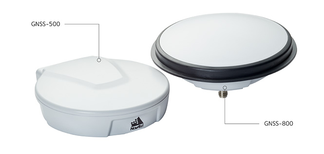
Neil Gerein, Portfolio Manager, NovAtel. (Photo: NovAtel)
Neil Gerein
Director, Product Management, NovAtel
At NovAtel we often say, “accuracy is addictive,” and to meet increasingly demanding accuracy and reliability requirements it is vital to concentrate on the antenna. After all, the antenna is the first in a long chain of key technologies that the GNSS signals must pass through to create a position, navigation and timing solution.
All modern GNSS transmit on multiple frequencies, with wide bandwidth signals, requiring antenna elements and integrated low noise amplifiers (LNAs) that operate across these frequencies. The challenge is to design the antenna element and LNAs for symmetric radiation patterns across all frequencies while minimizing multipath, phase center offset (PCO) and phase center variation (PCV). The result is better carrier-phase measurements, and therefore more accurate solutions in real-time kinematic (RTK) and PPP applications.
Photo: NovAtel
Since 2016 the Radio Equipment Directive (RED) has been in effect, and all GNSS receiver systems sold into the European Union must be compliant to the standard, including adjacent-band compatibility and spurious emissions testing. RED compliance is an end-to-end system test, where the filtering within the antenna must be analyzed in concert with the filtering capabilities of the connected GNSS receiver to meet the requirements. The antenna performance therefore becomes critical to any GNSS receiver system that is intended to be sold within the EU.
Gyles Panther, president and CTO, Tallysman Wireless. (Photo: Tallysman)
Gyles Panther
President and Chief Technical Officer, Tallysman
A fact often not appreciated is that the performance of a GNSS antenna is commonly the limiting factor in system accuracy. Digital signal algorithms in the receiver are helpful, but if the signal delivered by an antenna is less than optimum, the receiver cannot compensate.
Precision GNSS systems typically rely upon resolved wavelength ambiguity measurements, combined with ephemeris and clock corrections to determine signal time of flight. In real-time kinematic (RTK) and precise point positioning (PPP) receivers, the basis for this measurement is phase locked tracking of received satellite signals. Thus an over-arching measure of antenna performance in the specific application conditions is the proportion of the time that phase lock is maintained by the receiver.
The VeraChoke GNSS antenna. (Photo: Tallysman)
All this provides for an unprecedented level of accuracy, with precision antennas now more akin to the ends of a tape measure than providing a simple GNSS “fix.” To this end, key parameters include a best possible G/T ratio, high multipath rejection, excellent axial ratio, high front-back ratio and minimal phase-center variation (PCV), all with high uniformity in the azimuth — altogether a very demanding design task.
Combining these parameters to provide exquisite accuracy, the Tallysman VC6100 choke ring antenna has less than 1 millimeter PCV when combined with absolute calibrated corrections data, whilst the lower cost VP6000, with its less complex installation, can be used without corrections data and still be within a millimeter or two of the truth compared to its more precise cousin.
Q: What is the GNSS/PNT industry “Issue of the Year”?
Jose Angel Avila Rodriguez, signal and security implementation engineer, European Space Agency
A: The growth of PNT applications has been impressive and will continue. Assurance of PNT will thus gain an ever-increasing role, in both the security and the civil domains.
For GNSS, the key PNT contributor, there is in addition another challenge: its piece in the PNT cake will be contested by newcomers, such as telecom networks. Whether we will continue talking about A-GNSS or instead talk about Assisted 5G, with GNSS in that case taking on the role of signal of opportunity — that will depend on today’s decisions about future GNSS upgrades, the modernized versions of Galileo second generation, GPS III, and Beidou/Compass III, that will be flying around 2040.
Gyles Panther, president and CTO, Tallysman Wireless, Inc.
A: The key issues for PNT going forward, and into the indefinite future, are simply stated: availability and accuracy. Re-deployment of the eLoran infrastructure is a no-brainer. A potentially highly negative step would be the introduction of communication services within the mobile satellite L-band downlink frequency band (1525 MHz to 1559 MHz). Multi-constellational receivers track a much larger number of satellites and better disposed SVs (space vehicles) provide a lower horizontal DOP and hence greater accuracy.
Finally, GNSS needs to be defended against interference both intentional and accidental. Why on earth would we want to damage something that is providing so much utility to mankind?
Small ceramic patch elements offer nearly perfect single-frequency receive characteristics and have become the standard for GPS L1 antennas. However, the new generation of GNSS receivers now being introduced track many satellites in multiple constellations. Are these narrow-band devices up to the task for wider bandwidths?
L1 Compass and GLONASS navigation signals are broadcast on frequencies close to GPS L1, but the offset exceeds the circular-response bandwidth of small patch antennas. This article discusses the nature of the defects to be expected with the use of small patches over the broader bandwidths required, and contrasts this with the higher performance of dual-feed patch antennas.
It is very difficult to evaluate the relative merits of GNSS antennas without very specialized equipment and resources. An accurate method for comparative evaluation of competing antennas is described that makes use of the C/N0 values reported by GNSS receivers.
A particular challenge facing GNSS is the threat posed by encroaching interfering signals; the LightSquared terrestrial segment signals often being quoted. Relatively simple measures are described to make GNSS antennas immune and the small resulting hit to antenna performance is quantified.
Circularly-Polarized Carrier Signals
The civilian signals transmitted from GNSS satellites are right hand circularly polarized (RHCP). This allows for arbitrary orientation of a receiving patch antenna (orthogonal to the direction of propagation) and, with a good co-polarized antenna, has the added benefit of cross polarization rejection.
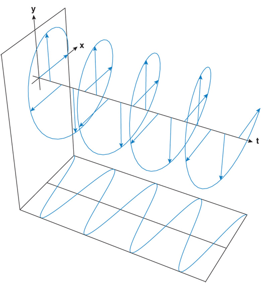
For conceptualization, circularly polarized (CP) signals can be thought of as comprised of two orthogonal, linearly polarized signals offset in phase by 90 degrees, as shown in fig 1 below. With one feed defined as I (in-phase), and the other Q (quadrature), the response of the antenna will either be LHCP or RHCP depending upon the polarity of the Q signal phase relative to that of the I signal.
If a CP signal is reflected from a metallic surface (such as metalized glass), the reflected signal becomes cross-polarized, so that a reflected RHCP signal becomes LHCP, and vice-versa. Unlike the linearly polarized (LP) case, a good CP receiving antenna will reject cross-polarized signals resulting from a single reflection. In this respect, reception of CP signals by a CP antenna is considerably improved relatively to linearly polarized signals.
FIGURE 1. Graphic representation of circular polarization (from Innovation column, July 1998 GPS World).
Frequency Plans
At this time, four global navigation satellite systems (GNSS) are either in service or expected to achieve full operational capability within the next 2–3 years: GPS, of course, GLONASS, also now fully deployed, Galileo, and Compass, expected to be deployed over the next two years.
Thus the systems and signals to be considered are:
GPS-L1 at 1575.42 MHz;
GLONASS L1, specified at 1602MHz (+6, –7) × Fs, where Fs is 0.5625 MHz;
Compass at 1561 MHz;
Galileo L1 as a transparent overlay on the GPS system at 1575.42 MHz.
It has emerged that considerable accuracy and availability benefits derive from tracking a larger number of satellites from multiple constellations. Notably, STMicroelectronics has produced an excellent animation of the GPS and GLONASS constellations that shows the theoretical improvement in accuracy and fix availability that derive from simultaneously tracking GPS and GLONASS satellites in Milan, For a really interesting comparison check out www.youtube.com/watch?v=0FlXRzwaOvM.
Most GNSS chip manufacturers now have multi-constellational GNSS receiver chips or multi-chip modules at various stages of development. It is awe-inspiring that the navigational and tracking devices in our cars and trucks will in the very near future concurrently track many satellites from several GNSS constellations. Garmin etrex 10/20/30 handhelds now have GLONASS as well as GPS capability.
Small single-feed patch antennas have good CP characteristics over a bandwidth up to about 16 MHz. This format is cheap to build and provides almost ideal GPS L1 characteristics.
Multi-constellation receivers such as GPS/GLONASS require antennas with an operational bandwidth of up to 32 MHz, and up to 49 MHz to also cover Compass.
Patch Antenna Overview
The familiar patch element is a small square ceramic substrate, fully metalized on one side, acting as a ground plane, and on the other, a metalized square patch. This structure constitutes two orthogonal high-Q resonant cavities, one along each major axis. An incident circular electromagnetic wave induces a ground current and an induced voltage (emf) between the patch edge and ground plane so that at resonance, the cavity is coupled to free space by these fringing fields.
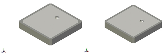
A typical low-cost GPS L1 patch is a 25 × 25 × 4 mm block of ceramic (or smaller) with a single-feed pin. Patches as small as 12 mm square can be fabricated on high-dielectric constant substrates, but at the cost of lower gain and bandwidth. The two axes are coupled either by chamfered patch corners or by offset tuning plus diagonal feed pin positions (Figure 2).
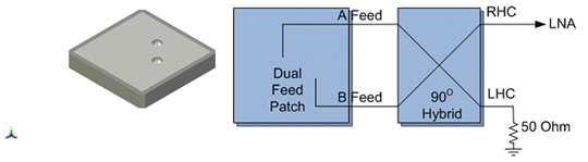
An alternate form of patch antenna has independent feeds for each axis. The feeds are combined in a network that fully isolates the two feeds. Dual-feed antennas can provide nearly ideal characteristics but are inherently more expensive to build. See Figure 3.
FIGURE 3. Dual-feed patch (left) and feed combiner (right).
Basic Performance Parameters
The factors that have a direct bearing on patch performance are:
Gain and radiation pattern;
Available signal-to-noise as a function of receiver gain and low-noise amplifier (LNA) noise figure;
Bandwidth, measured as: radiated power gain bandwidth; impedance bandwidth; or axial ratio bandwidth.
Gain and Radiation Pattern. Patch antennas are specified and usually used with an external ground plane, typically 70 or 100 millimeters (mm) square. Without an external ground plane a reasonable approximation of the radiation pattern is a circle tangential to the patch ground plane with a peak gain of about 3 dBic (dBic includes all power in a circular wave). The addition of an external ground plane increases the peak gain at zenith by up to 2 dB.
The pattern shown in Figure 4 is typical for a 25 mm patch on a 100 mm ground plane. The gain peaks just under 5 dBic, dropping to about 0 dB at an elevation angle of ±60 degrees (the horizon is 90 degrees).
FIGURE 4. Radiation pattern for 25 mm patch on 100 mm ground plane.
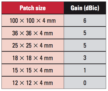
Table 1 tabulates approximate gain values at zenith for a range of GPS L1 patch sizes, mounted on a 100-mm ground plane, at resonance, radiated with a RHCP signals (that is, dBic).
TABLE 1. Patch size versus gain at zenith.
Clearly, gain is significantly lower for patches smaller than 25 mm square. Not illustrated here is that the bandwidths of antennas smaller than 25 mm also become too narrow for consideration for anything other than single-frequency signals such as GPS L1.
Achievable C/N0. The carrier signal-to-noise density ratio (C/N0) is a fundamental measure of signal quality and hence antenna performance. For a given receiver, if the C/N0 is degraded due to any cause, be it a poorly tuned patch or bad LNA noise figure or other, the shortfall in performance is non-recoverable.
The effective isotropic radiated power (EIRP) of the transmitted GPS L1 signal from the space vehicles is approximately 27 dBW. If D is the range to the satellite, and λ is the carrier wavelength, the free space path loss, PL, is given by
PL = [ λ / (4 × π × D)]2
The signal power received at the antenna terminals, Pr, is given by:
Pr = EIRP × Gr × PL
where Gr is the receive antenna gain.
The noise power in a 1 Hz bandwidth, N0, referred back to the antenna terminals is given by:
N0 = 10log(Te × k),
where Te is the overall system noise temperature, and k is the Boltzmann constant.
Thus C/N0, the ratio of received carrier power to noise in a 1 Hz bandwidth, referred to the antenna is
C/N0 = Pr / N0
Quantifying this calculation: For λ = 0.19 meters (corresponding to the L1 frequency), and an orbit height of 21,000 kilometers, the path loss,
PL = –182.8 dBW.
The received signal power,
Pr = EIRP(dBW) + Gr(dB)+ PL(dB)
(in dBW)
Assuming the mid-elevation antenna gain, Gr, is 3 dBic,
Pr = –152.8 dBW.
For a cascaded system such as a GPS receiver, the overall noise temperature is given by:
Te = Ts + Tlna + Tgps/Glna
where Te is the overall receiver system noise temperature, Tsis an estimate of sky-noise temperature at 1575.42 MHz, assumed to be 80 K, Tlna is the LNA noise temperature (76 K for an LNA noise figure of 1 dB), Glna is the LNA gain (631 for 28 dB gain), and Tgps is the noise temperature of the GPS receiver (636 K for 5 dB receiver noise figure).
Thus, Te = 157.1 K and N0 = –206.6 dBW.
The available ratio of received carrier power to 1 Hz noise, C/N0, referenced to the antenna is:
C/N0 = Pr/(Te × k) –
(implementation loss)
where implementation loss is an estimate of the decode implementation loss in the GPS receiver, assumed to be 2 dB (something of a fiddle factor, but reasonable!)
Thus, C/N0 = –152.8 – (–206.6) – 2 dB = 51.8 dB.
For satellites that subtend a high elevation angle, the reported C/N0 could be 2 dB higher or 53.8 dB best case.
A good circular antenna should provide C/N0 values in the range 51 dB–53 dB. This can be checked using the (NMEA) $GPGSV message output from most GNSS receivers. Comparative measurement of C/N0 provides the basis for comparative antenna evaluation as described later.
Single-Feed Bandwidth. Bandwidth of single-feed patches can be defined in several quite different ways.
Radiated power gain bandwidth: the bandwidth over which the amplitude at the terminals of the receiving antenna is not more than X dB below the peak amplitude, with an incident CP field.
Axial ratio bandwidth: the bandwidth over which the ratio of the maximum to minimum output signal powers for any two orthogonal axes is less than Y dB. This is an indicator of how well the antenna will reject cross-polarized signals.
Return loss (RL) or impedance bandwidth: that over which the feed input return loss is less than Z dB. This is very easy to measure, and gives the most optimistic bandwidth value.
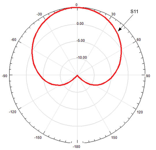
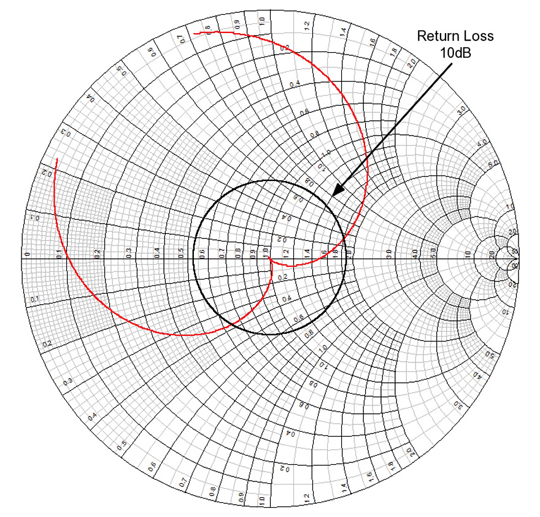
The input impedance of a single-feed patch is shown in Figure 5. The rotated W-shape of the single-feed patch impedance is a result of the coupling between the two axes of the patch. The 10 dB return loss, called S11, is shown as a circle, outside of which |S11| > –10 dB.
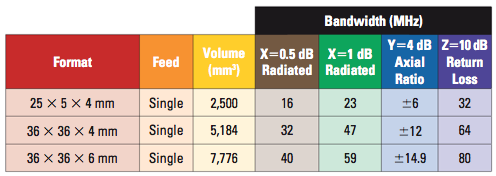
These measures of bandwidth are shown for 25 × 25 × 4 mm and two thicknesses of 36 mm2 antennas in Table 2.
FIGURE 5. S11 for a 25 mm single-feed patch.TABLE 2. The various measures of patch bandwidth.
These different measures yield large differences in bandwidth. The merits of each depends on what is important to the user.
From a purist viewpoint, the most intuitively useful measure of bandwidth is the 0.5 dB radiated gain value. Even then, at the band edges so defined, the axial ratio for a 25 mm2 × 4 mm patch is degraded to about 5 dB, just on the negative side of ok.
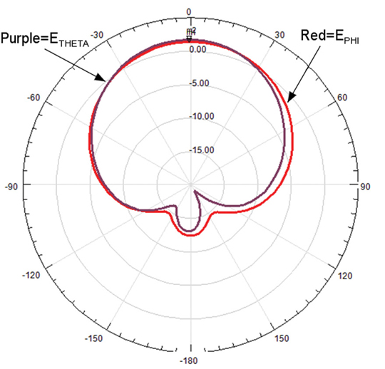
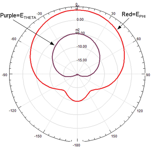
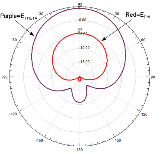
As shown in Table 2, the 10 dB return loss bandwidth is comparatively wide. Figure 6 shows the EФ and Eϴ fields for a 36-mm patch a) at resonance and, b) and c), at the upper and lower –10 dB RL frequencies. At resonance the fields are equal, and the radiation is circular (add 3 dB for the CP gain). At the two 10 dB RL offset frequencies, the axial ratio is about 9 dB, with the dominant axis swapped at the band edges.
(a)
(b)
(c) FIGURE 6. (a) Realized gain patterns EФ and Eθ, single-feed at resonance, Fc. (b) realized gain patterns EФ and Eθ , single-feed, Fc+F–10 dB.
(c) realized gain patterns EФ and Eθ, single-feed, Fc-F+10dB.
As a transmitter, a 10 dB return loss would correspond to 90 percent of the energy transmitted, in this case, mostly on a single axis. By reciprocity, as a receiver, the single axis gain of the patch at the 10 dB RL frequency is higher (by about 2 dB ) than at resonance. So, if a linear response can be tolerated, the 10 dB bandwidth is a useful measure, albeit for a very non-ideal response.
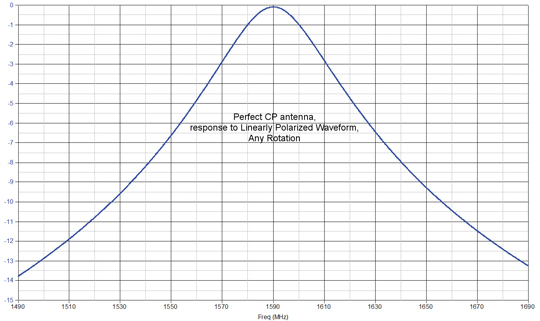
Because the two axes are only balanced at resonance, single-feed patches are only truly circular at resonance. An ideal CP antenna has an equal response to a linearly polarized signal, for any rotational angle of incidence. Figure 7 shows the response of a CP antenna to a LP signal for any rotation, which is 3 dB down relative to the response to a co-polarized CP wave.
Figure 7. Perfect CP response to linearly polarized waveform.
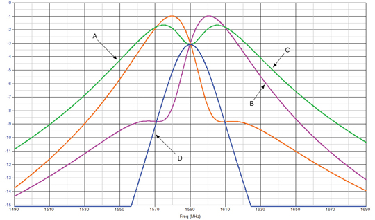
In contrast, Figure 8 shows the responses of a single-feed patch (25 mm2 × 4 mm) as a function of field rotation with a linearlarly polarized wave. Note that, at resonance, all of the responses have the same amplitude because the patch is circular at that frequency.
Figure 8. 25-millimeter single-feed patch response to linear polarization rotation.
The responses shown above are for the following conditions:
A) single axis excitation (axis A)
B) single axis excitation (axis B)
C) equal axis excitation, antipodal
D) equal axis excitation, in-phase.
The relevance of this is that a circular polarized wave can become elliptical as a result of multipath interference. Figure 8 shows that the antenna response can be highly variable as a function of the angle of the ellipse principal axis. This is another way of looking at impaired cross-polarization rejection.
In addition, poor axial ratio results in non-equal contributions from each of EФ and Eϴ as the E vector of a linearly polarized wave is rotated. Thus an antenna with a poor axial ratio has a non-linear phase response, unlike a truly CP antenna which has an output phase that rotates proportionally with the E vector rotation.
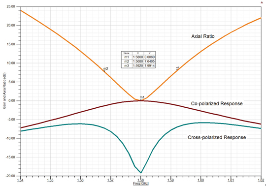
25 mm2 patches for GPS/GLONASS applications are tuned to the mid frequency of 1590 MHz. Because the RHCP response is narrow, so is the cross polarization rejection, which is also centered at 1590 MHz, Figure 9 shows the simulated response of a single-feed 25 mm patch to co-polarized and cross polarized fields.
Figure 9. Co-polarized and cross polarized response, single-feed patch.
The cross-polarization rejection is degraded at both GPS and GLONASS frequencies, so that much of the ability of the antenna to reject reflected signals is lost.
Against these criteria, a 25 × 25 × 4 mm single-feed patch element can provide good CP performance over about 16 MHz. Of course, initial tuning tolerance must be subtracted from this. However, even within the 0.5 dB radiated gain bandwidth the axial ratio rapidly becomes degraded to about 5 dB, and at larger offsets, the patch response becomes virtually linearly polarized, with poor cross-polarization rejection and phase response. However, as a redeeming feature, the single-feed patch has a wideband frequency response albeit linearly polarized at the GPS and GLONASS frequencies (the band edges).
Dual-Feed Patches
By comparison, dual-feed patches can provide almost ideal characteristics over the bandwidth of the patch element. Figure 3 shows a typical physical configuration and a schematic representation for the feed combining network. This ensures that the two axis feeds are fully isolated from each other over all frequencies of interest. The well known 90-degree hybrid coupler provides exactly the required transfer function.
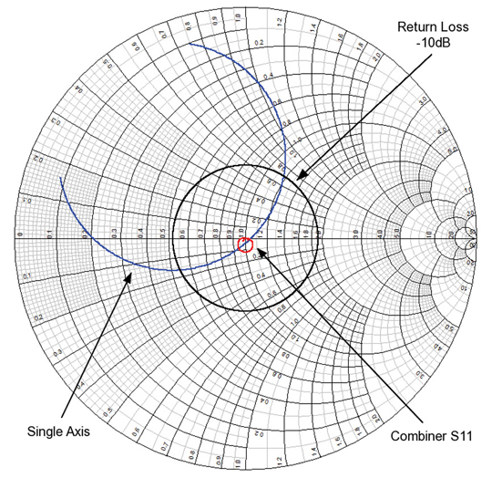
The Smith chart in Figure 10 shows the impedance of one of the two feeds (that is, one axis) and the combiner output impedance, this being just a small locus close to 50 ohms.
Figure 10. Dual-feed patch, single axis and combiner S11.
Contributions from each axis at all frequencies are theoretically identical for a perfect specimen, so that the configuration naturally has an almost ideal axial ratio (0 dB).
Gain and Radiation Pattern. At resonance, the mode of operation of the single and dual-feed patches is identical so, unsurprisingly, the gain and radiation pattern are also the same; see Figure 4.
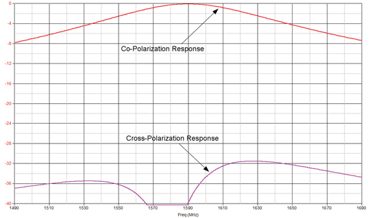
Dual-Feed Bandwidth. The 1 dB radiation bandwidth of a dual-feed patch is just less than 1 MHz narrower than if configured as a single feed. Otherwise, the bandwidth of a dual-feed patch is simply the resonant characteristic of the cavities comprised of each axis. The allowable in-band roll-off defines the patch bandwidth, which in any event should not be worse than 1.0 dB, including initial tuning errors. The response for a 36 × 36 × 6 mm patch is shown in Figure 11.
Figure 11. Co-polarization and cross-polarization response, dual-feed patch.
Axial Ratio. Because the axial ratio of dual-feed patches is inherently good, the cross-polarization rejection is also good. The simulated cross-polarization response for the dual-feed patch is also shown in Figure 11.
In reality, small gain and phase imbalances in the printed circuit board, hybrid coupler, and patch itself will prevent the axial ratio from being perfect and cross-polarization response not quite so ideal. With good manufacturing controls, axial ratio can be held to typically better than 2 dB.
The obvious question is, since dual-feed devices have nearly ideal characteristics, why not just make a low cost small dual-feed antenna? There are three issues: The first is that the feed offsets required for a 25 mm2 patch are physically too close for two feed pins. Secondly, a dual-feed structure requires an additional relatively expensive combiner component; thirdly, sometimes, the only way to achieve the necessary bandwidth is through the considerably extended, but linearly polarized bandwidth of the single-feed patch.
That said, were it possible, it would be the ideal solution.
Comparative Performance
The C/N0 value reported in the NMEA $GPGSV message provides a simple method for comparative evaluation of GNSS antennas. The idea is to compare reported C/N0 values for a number of competing antenna types.
This requires a reference GPS receiver, a logging computer and the antennas to be evaluated, and these should be arranged so that:
The computer is set up to log the NMEA $GPGSV messages output from the receiver ($GLGSV for GLONASS).
Each antenna is placed and centered on identical ground planes (100 mm),
The antennas-under-test are not closer to each other than 0.5 meters (to ensure no coupling), and
Each antenna-under-test has a clear sight of the whole sky, and
It is possible to quickly switch the antenna connectors at the receiver.
The method is to connect each antenna in sequence for 15 seconds or so, and to log NMEA data during that time. The antenna connector substitution should be slick, so that the receiver quickly re-acquires, and to validate the assumption of a quasi-stationary constellation.
Each NMEA $GPGSV message reports C/N0, at the antenna, for up to 4 satellites in view. The best reported average C/N0 value for specific satellites 49 dB and above are the values of interest. The winner is the highest reported C/N0 value for each constellation.
This sequence should be repeated a few times to get the best estimate. The important parameter is the difference between the reported C/N0 and the receiver acquisition C/N0 threshold. If the acquisition C/N0 threshold is –30 dB, an antenna that yields –49 dB C/N0 has a 19 dB margin, while an antenna that yields 52 dB has a 22 dB margin — a big difference.
Immunity to LightSquared
Much has been written regarding the threat of the prospective terrestrial segment that the LightSquared L-band communication system poses for GPS (and GNSS in general), which mostly is true. On the other hand, front-end protection for GNSS antennas is a relatively simple, inexpensive addition. The performance cost (in addition to a very small dollar cost increment) is an unavoidable but relatively small sensitivity hit. Note that L-band augmentation systems, other than WAAS and compatible systems, face a more difficult problem.
This is not just a LightSquared issue. In several corners of the world, transmission of high-level signals are permitted that have the potential to interfere with GPS either by source distortion or inter-modulation within the GPS antenna front end itself.
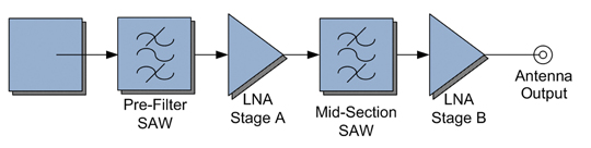
The primary hazard is saturation of the first stage of what is usually a two stage LNA. So, the only way to protect against this is a pre-filter, as shown in Figure 12.
FIGURE 12. Pre-filtered antenna architecture.
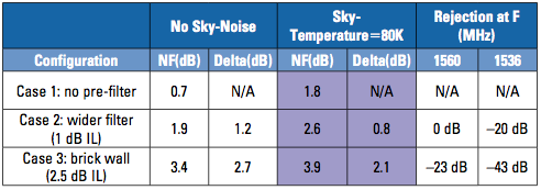
There is a trade-off between the slope and corner frequency of the pre-filter out-of-band rejection and its associated insertion loss. The table below shows the response with a wider filter with an insertion loss of 1 dB, the second a more aggressive filter with a 2.5 dB insertion loss (IL).
Table 3 shows overall noise figure including and excluding sky noise. Sky-noise temperature is used here as a catchall that includes true sky-noise, thermal noise (the antenna can partially see the local environment), plus similar factors. The value used is arguable, but experience indicates this is a reasonable number.
The existence of sky noise limits the lowest available noise figure and sets the effect of a pre-filter in the correct context. In any event addition of a quite adequate pre-filter against a 1536 MHz signal can be achieved with less than 1 dB impact on received C/N0.
TABLE 3. Rejection and noise figure for pre-filtered antenna.
Putting It All Together
Small (25 mm2 × 4 mm) single-feed patches are only truly circularly polarized at resonance but do have good CP characteristics over a bandwidth of about 16 MHz, and almost perfect for GPS L1. The pre-dominance of this format for GPS L1 is fully justified.
However, when used to receive wider bandwidth signals such as GPS/GLONASS, single-feed patch antennas suffer from a litany of minor flaws, most particularly poor axial ratio and poor cross-polarization rejection.
On the other hand, the coupling that happens in single-feed antennas results in a very wide 10 dB return loss bandwidth but at the band edges (where the GNSS signals are) they are virtually linearly polarized.
There is no doubt that the performance of small single-feed patches for bandwidths such as those required for GPS/GLONASS coverage is marginal. However, to no small extent, the sensitivity of modern receiver chips is so good that marginal antenna performance can often be accommodated, at least from a basic operational viewpoint. The receiver bails out the antenna.
However, the end result must be degraded GNSS reception. If the application cannot tolerate reduced GNSS availability or accuracy because of marginal antenna performance the choice should be a dual-feed patch type. This will present the GNSS receiver with more consistent signals levels and phase responses and less interference. The end result should be faster acquisition, and realization of the improvement in horizontal dilution of precision (HDOP) that GPS/GLONASS offers.
The reported values of C/N0 in the $GPGCV NMEA message provides a simple and sensitive means to comparatively evaluate antenna performance.
A not insignificant consideration is that the antenna is usually a very visible part of a bigger system, and unavoidably represents the quality of the user equipment. In that case, the antenna housing robustness and appearance may also be a criterion to maintain the image of the end product.
The final point is that introduction of pre-filters into active GNSS is a good idea, whose time has come. This provides protection against the well known bug-a-boo, but also protects against known interference in other parts of the world.
Acknowledgments
I would like to acknowledge the assistance of Inpaq Technologies (Suzhou) Ltd., for provision of patch samples and technical support; Rony Amaya, adjunct research professor, Carleton University, Ottawa, for discussions and assistance in preparing this article; and STMicroeletronics for permission to cite the GPS+GLONASS demonstration video.
Gyles Panther is president and CTO of Tallysman Wireless (www.tallysman.com) and has an honors degree in applied physics from City University, London. He has worked in the fields of RF and satellite communications for more than 20 years. As CTO of a precursor company he was the principal engineer for the development of a wide-area Canadian differential GPS corrections system (CDGPS) receiver. Tallysman is a new start-up specializing in high-performance GNSS antennas and systems.