Tag: Newark Airport

  • Jammer Hunting with a UAV

    A fully autonomous, unmanned aerial vehicle (UAV)-based system for locating GPS jammers, currently under development, seeks to localize a jammer to within 30 meters in less than 15 minutes in an area comparable to that of an airport. Ultimately, the design team targets the ability to locate multiple, simultaneous jammers, and navigate in intermittent GPS and GPS-denied environments using a combination of GPS and alternate navigation aids. The system should be inexpensive and built from commercially available or open-source parts and software.

    By James Spicer, Adrien Perkins, Louis Dressel, Mark James, Yu-Hsuan Chen, Sherman Lo , David S. De Lorenzo and Per Enge, Stanford University

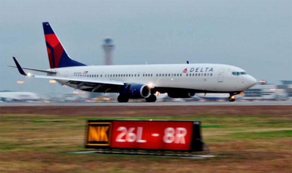
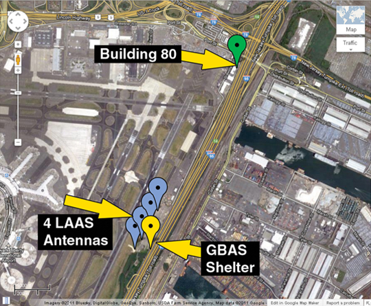
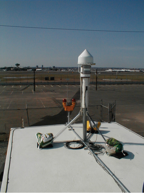
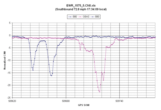
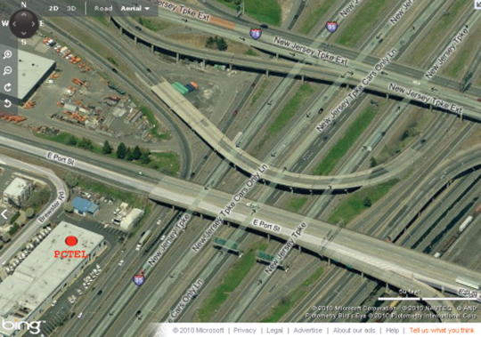
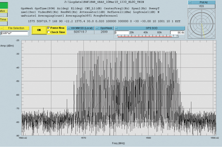
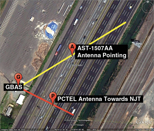
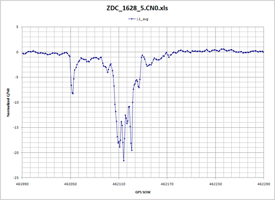
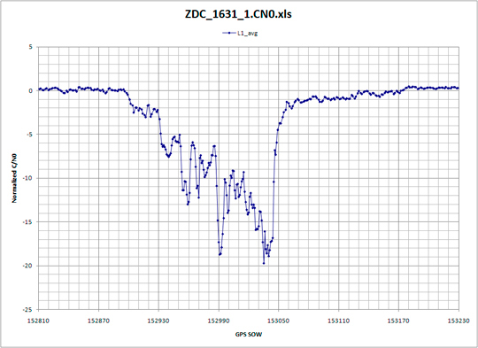
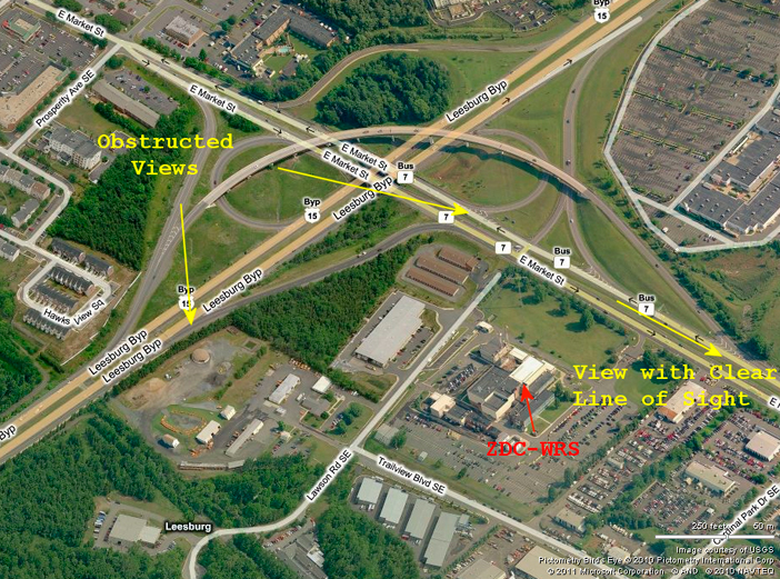
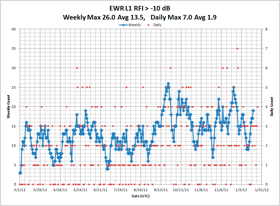
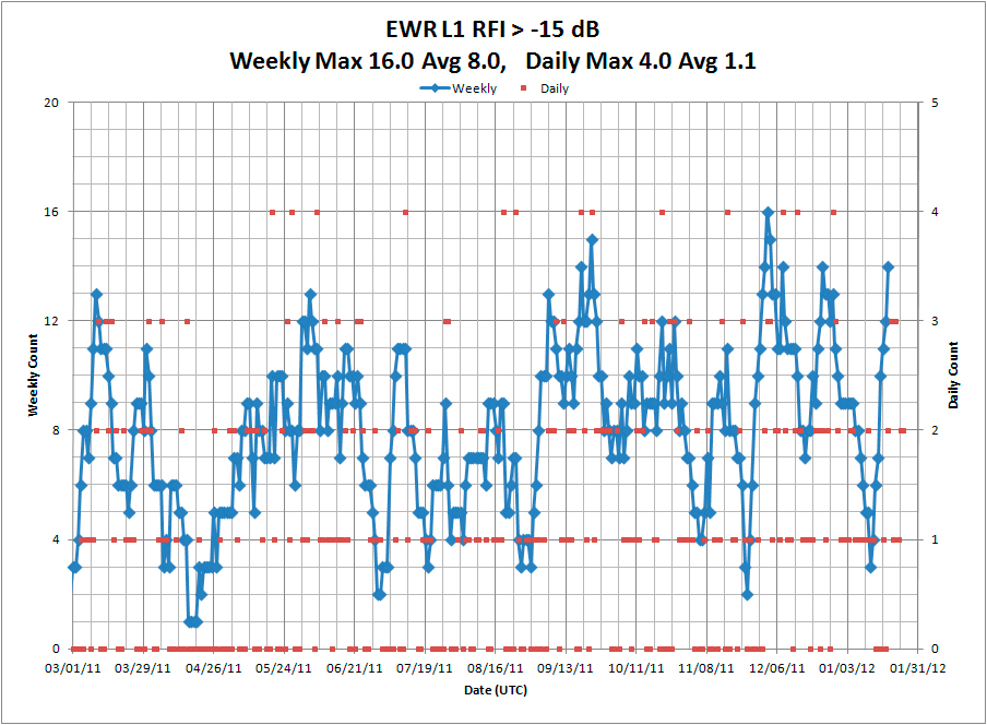
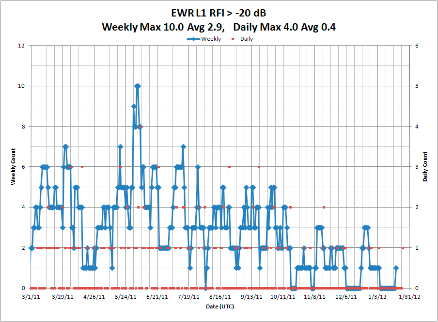
    The aviation community worries about GPS jamming. Recently, it struggled to find so-called personal privacy devices on Newark’s Liberty International Airport and traveling the nearby New Jersey Turnpike.

    A number of unintentional jamming incidents took a long time to resolve. The disruption from an intentional, malicious jamming attack could be far worse. Airport authorities should be prepared to locate and shut down a coordinated attack by numerous jammers capable of disrupting the GPS service over an entire airport.

    The closure of a major airport for the many hours or days it would take to locate even a couple of backpack-sized transmitters would be not only be highly disruptive in flights delayed or diverted, it would negatively impact the confidence of the flying public.

    Any system in place to mitigate this threat must be inexpensive enough to be deployed at least at the nation’s major commercial airports, autonomous enough to be operable with limited training and certification, and rapid and accurate enough that a jammer can be routinely apprehended by ground-based law enforcement. It must be able to navigate successfully in GPS-denied environments using alternative position, navigation and timing (APNT), and have the range and capacity to search an airport-sized area as well as the approach corridor leading to runway touchdown.

    This article describes such a system and device presently in research and development: the Jammer Acquisition with GPS Exploration & Reconnaissance (JAGER).

    Vehicle Design and Operation

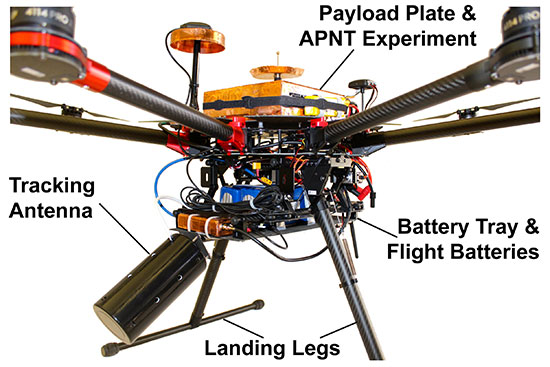
    The JAGER UAV is a based on a commercially available, multi-rotor airframe modified to suit the mission specifications. The 1.2-meter diameter octocopter has a maximum takeoff weight of 11 kilograms (24.2 pounds), a top speed of 20 meters/second (m/s, 45 mph), and can fly unloaded for up to 30 minutes.

    We have replaced the battery tray with our own carbon fiber design that allows us to carry 16 Ah of lithium polymer batteries for a maximum power draw of 4 kW. This extra capacity means that even with a 5-kilo experimental payload, the present craft can remain aloft for up to 15 minutes without recharging.

    The payload plates are also custom-made from carbon fiber, and it is to these that the UAV’s experimental payloads are mounted (see FIGURES 1 and 2). One payload plate is flown at a time, and is secured on top of the airframe with a quick-release mechanism. This modularity allows for individual experiments to be mounted to their own payload plate and ground-tested before being secured to the UAV. Different experiments can be switched out rapidly for efficient use of battery capacity and flight time.

    Figure 1. (A) Diagram of the payload plate showing regularly spaced mounting holes. (B) Plate with APNT experiment mounted. (C) Payload plate / experiment assembly secured atop JAGER UAV.
    Figure 1. (A) Diagram of the payload plate showing regularly spaced mounting holes. (B) Plate with APNT experiment mounted. (C) Payload plate / experiment assembly secured atop JAGER UAV.
    Figure 2. Image of the vehicle showing the battery tray slung beneath the central body, the APNT experiment and payload plate secured on top, and the jammer-hunting antenna mounted at the front.
    Figure 2. Image of the vehicle showing the battery tray slung beneath the central body, the APNT experiment and payload plate secured on top, and the jammer-hunting antenna mounted at the front.

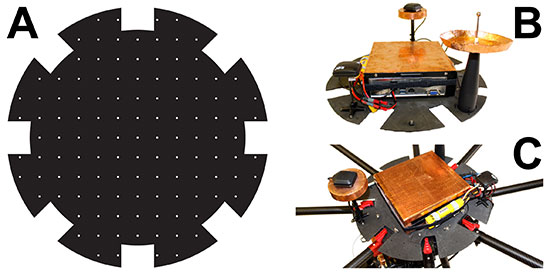
    The plate itself also offers flexibility for component mounting. Regularly spaced, threaded holes across the plate mean components’ positions can be easily changed to find an optimal configuration. This can be particularly useful for minimizing interference between computers and noise-sensitive components such as antennas and magnetometers.

    Software. We modified existing, open-source autopilot software to fly the mission. The craft is fully capable of completing a mission autonomously, but also can be taken over by a human pilot if necessary. A ground station also can be used to send commands to the octocopter, but is primarily used to monitor UAV location, battery life, and jammer belief state.

    The autopilot software also has been adapted to communicate with various vehicle payloads. Experiments using APNT equipment, for example, pass their data to the autopilot, which will combine these signals with its own GPS data for accurate navigation in areas where the GPS signal might be intermittent or unreliable. In return, the autopilot can be used to pass data to experiments reliant on altitude, attitude, atmospheric pressure or location information.

    The ground station monitors instruments’ data and status in real time. This not only allows for control of airborne experiments, but also straightforward ground testing. Synthetic autopilot data can be fed to an experiment to ensure that all systems are performing correctly before they are mounted on the vehicle for flight tests.

    APNT Overview

    Key to navigating in a GPS-denied environment is the use of signals from APNT networks for location determination. The proposed system should be able to navigate using any or all available APNT signals, and should weight each one according to its strength and reliability in order to formulate the most accurate estimate of both its own and the jammer’s position.

    Here we describe the use of the universal access transceiver (UAT) and distance measuring equipment (DME) network for our APNT signals. The UAT signal has been implemented by the Federal Aviation Administration (FAA) in the United States as part of automatic dependent surveillance–broadcast (ADS-B), and is transmitted through a network of terrestrial ground stations.

    The ADS-B network was only completed across the contiguous United States in 2014, so it is new compared to established cellphone networks. It is more comprehensive than many other terrestrial systems, so that coverage of most airports is guaranteed. While GPS reception requires an unobstructed view of the sky, UAT reception requires a direct line of sight to a transmitting tower. However, the flatness of terrain surrounding most airports as well as the UAV’s airborne vantage point ensures that UAT signals will probably be visible throughout most jammer-seeking missions.

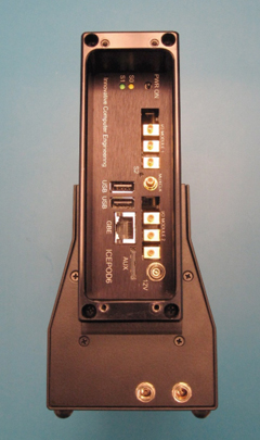
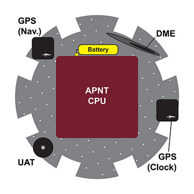
    The APNT equipment used for navigation by the JAGER UAV consists of UAT (978 MHz), DME (982 to 1213 MHz), and GPS (1575.4 MHz) antennas, a multichannel transceiver to combine the two signals, and a computer for data processing (see FIGURE 3). A dedicated lithium-ion battery powers the entire APNT payload. The current system does incorporate GPS to estimate the time offset, but future iterations of the system will derive time from sources other than GNSS so that true GPS-denied navigation is possible.

    Figure 3. Schematic of the APNT configuration on board the JAGER UAV. Resulting location information is passed to the autopilot for navigation.
    Figure 3. Schematic of the APNT configuration on board the JAGER UAV. Resulting location information is passed to the autopilot for navigation.

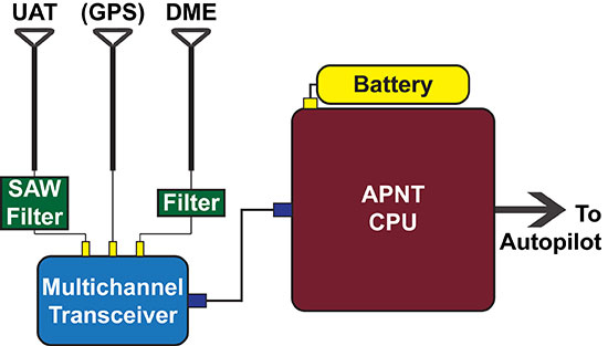
    The UAT antenna receives multiple signals from visible ADS-B ground station transmitters. The transceiver combines these with a GPS timestamp, and the data is passed to the APNT computer for analysis. Based on knowledge of the absolute locations of the ADS-B antennas, the range of the vehicle from each antenna can be calculated, which in turn can be used to trilaterate the vehicle’s absolute position. This position is then passed to the autopilot for the UAV’s navigation, while the status of the equipment and signal strength are passed down to the ground for monitoring in real-time.

    The necessity of using GPS signals as an accurate timing system is a current limitation, as navigation in GPS-denied conditions is clearly not possible while we are using GPS as a clock. As mentioned eariler, future designs will derive time from non-GNSS sources, such as chip-scale atomic clocks or the terrestrial ranging signals.

    Carrying an onboard computer allows for real-time processing of the terrestrial alternative navigation signals.  However, there are a few limitations to the use of these signals. First, the vertical position is difficult to calculate due to the geometry of terrestrial signals as well as the sparsity of visible station at low elevation. This is solved by using a baro-altimeter. Second, DME signals do not provide a pseudoranging function. Current work sponsored by the FAA is developing a DME pseudoranging capability. As the technology matures, we will improve the hardware and algorithm that can be integrated into future JAGER designs, resulting in lower weight and power overhead for the APNT payload.

    Tracking Overview

    GPS jammers do little more than emit signals in the GPS frequency range. Because the signals from GPS satellites are so weak by the time they reach the Earth, ground-based jammers do not have to be especially powerful to overwhelm GPS in their immediate vicinity. A jammer is no more than a ground-based radio-frequency source radiating within the GPS spectrum.

    The JAGER system will autonomously locate the nearest beacon emitting electromagnetic signals at the target frequency: the GPS frequency in this scenario. Testing such a system is difficult due to the illegality of jamming the GPS signal within the United States. We instead test the system using a powerful Wi-Fi beacon as a proxy for the overpowering jammer. Excepting the target frequency, the procedure to locate the jammer is identical to the GPS case.

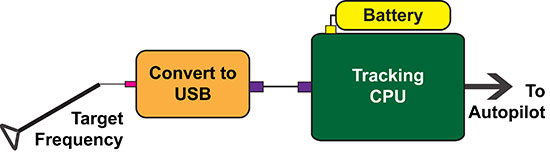
    To receive the jamming signal, the front of the craft carries an antenna optimized to receive signals of the target wavelength; the current antenna has a 60° cone of maximum sensitivity. It is angled downward 30° from the horizontal, so that the craft can receive all signals from the horizon to 30° from vertical. This gives the UAV visibility over most of the space in front and underneath it. Like the other payload equipment on the vehicle, the antenna is secured with a fast-release mechanism so that it can be easily swapped out if necessary. For Wi-Fi tracking, we use a Yagi antenna with 60° beamwidth and 9 dBi gain. In upcoming trials, we will test different antenna configurations (such as dual antennas, small antenna arrays, and directional antennas augmented with omni-directional antennas) to determine benefits of these different layouts.

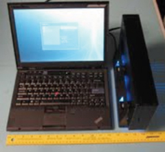
    Signals from the antenna are passed into a module that converts the Wi-Fi data to serial, then from serial to USB. A single-board Linux computer with a quad-core processor then analyzes the signal data (see FIGURE 4). The hardware used to locate the jammer weighs 160 grams, so has negligible impact on the vehicle’s flight time or range.

    Figure 4. Schematic of the tracking system on board the JAGER UAV. The resulting believed location of the target is passed to the autopilot.
    Figure 4. Schematic of the tracking system on board the JAGER UAV. The resulting believed location of the target is passed to the autopilot.

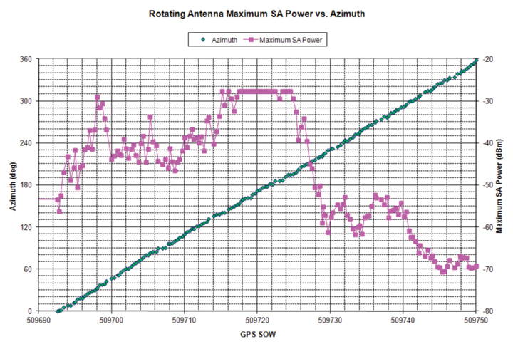
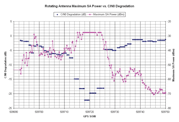
    To find the jammer’s location, the UAV performs a controlled yaw spin while recording the strength of the jamming signal. On the basis of the signal landscape surrounding the vehicle, the computer estimates the jammer’s location and sends a message to the autopilot instructing the craft to fly in that direction (or, more accurately, in a direction that optimally improves the ability of JAGER to find the jammer quickly). In return, the autopilot updates the tracking computer and ground station as to the vehicle’s position.

    After moving a certain distance towards the jammer’s believed location, the craft repeats the spinning maneuver and starts the process again. Although rotating only the antenna might increase the speed of the operation, the energy required to carry the necessary antenna-rotation mechanisms for the duration of a flight is more than that needed to spin the entire craft.

    The tracking algorithm is not as straightforward as gradient ascent or homing, and the vehicle will not always fly in the direction of greatest signal strength. The operational area is uneven, and may include buildings, towers, or airplanes, resulting in a complicated RF environment. Signals are scattered, diffracted and reflected, meaning that an algorithm that simply follows the strongest signal will not always converge on the actual jammer location.

    To decide the optimal path from the vehicle’s present location to the jammer’s believed position, the tracking algorithm makes use of partially observable Markov decision processes (POMDPs). POMDPs model decision processes where the underlying state of the system (that is, the location of the jammer) is never completely known, and maintain a probability distribution over the set of all possible states.

    The entire deployment area (an airport and its environs, for example) is split up into a square grid. For every possible combination of jammer and vehicle grid square locations, the signal strength and direction that would result is calculated offline prior to deployment and stored in a database on the tracking computer.

    During the mission, the UAV records its own position and the sensed jamming signal’s strength and direction. The jammer location that would correspond to this result is retrieved from the database, as well as a measure of the strength of this belief state.

    Once the craft has a belief as to the location of the jammer, it moves to a new location in the jammer’s believed direction before taking another measurement of signal strength. The new location and new measurement are combined, and the updated corresponding jammer location is retrieved from the database. This process is repeated until the vehicle believes itself to be right above the jammer, at which point a photograph is taken, the ground station is notified, and the hunting mission is complete.

    Having found the jammer, the system can be programmed to execute a wide range of operations. These include reporting coordinates and a live image of the believed jammer location back to the ground station, hovering above and tracking the jammer if it begins to move, landing at the jammer site, or returning to base.

    We calculate and store the POMDP decisions in advance of the flight. This strategy has some advantages. First, it allows for almost instantaneous decision-making. This is because the algorithm’s decisions are based solely on the vehicle’s current location and sensory observations and not on any previous states (a defining characteristic of a Markov decision process). The craft needs only to observe its current state in order to look up its next move in the database. This enables rapid tracking in flight.

    A second advantage is that safety checks can be pre-programmed into the database in advance of deployment. While JAGER is programmed to move towards the grid square believed to contain the jammer, it can also be programmed to avoid or take special precautions when moving towards or in the vicinity of certain squares in the grid (also called geo-fencing). In an airport situation, for example, the vehicle would avoid moving into the square containing a control tower or ground-based antenna, or would fly at a minimum altitude over buildings and taxiways to avoid collisions.

    Finally, the integration between the autopilot and the tracking software can provide other important safeguards: in the proof-of-concept system, any navigation decision taken by the software can be relayed to the ground for human verification before the UAV begins to move. This supervised mode of operation lends itself to a seamless migration path to fully autonomous operation (always overseen by a human operator).

    However, one disadvantage of calculating and storing decisions in advance is the storage space needed on the vehicle. Because the result of every possible combination of vehicle and jammer locations within the grid is calculated, the size of the database grows quickly with increasing numbers of possible positions (and states). The larger the grid or the greater the required accuracy, the more space is needed to store the database. With current algorithms, the database needed to locate a jammer to within 30 meters in an area the size of an airport requires 15 gigabytes of storage space, resulting in longer lookup times during flight.

    We are considering several strategies to mitigate this disadvantage, including better compression, more effective search algorithms, and uploading from a ground server only the parts of the database that correspond to the vehicle’s current operational area. Another strategy is to use an adaptive mesh that changes in resolution depending on the jammer’s belief state: at low certainty the database resolution is low, but increases in the appropriate area as the jammer’s location becomes more certain.

    Another disadvantage of pre-solving the decision-making process is that the system must be reconfigured for every site in which it is deployed. The specifications of the tracking algorithm will change depending on the requirements of the operating area. The grid size, shape and absolute location must change to suit the area being protected. The resolution of the grid depends on the required accuracy of the tracking system, and restricted or prohibited locations must suit the terrain, buildings and geological features of the deployment space. For example, a lead JAGER vehicle could be adapted and tested to suit a particular airport, and then the bespoke algorithm and database uploaded to backup vehicles in that airport’s fleet.

    APNT Performance

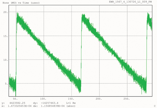
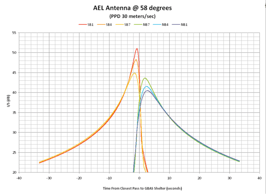
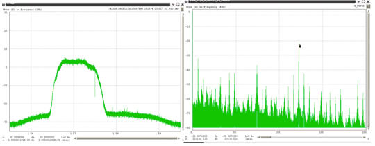
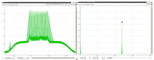
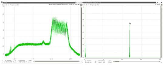
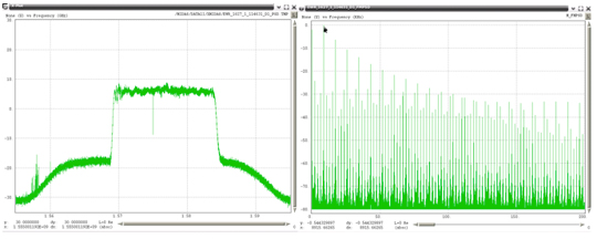
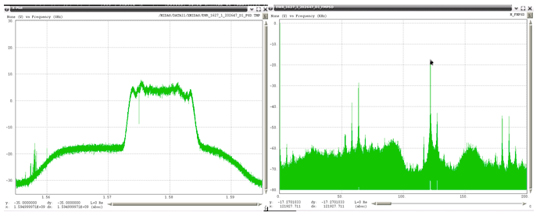
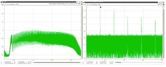
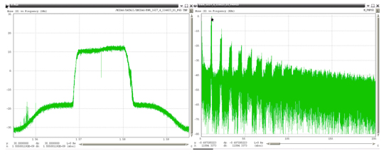
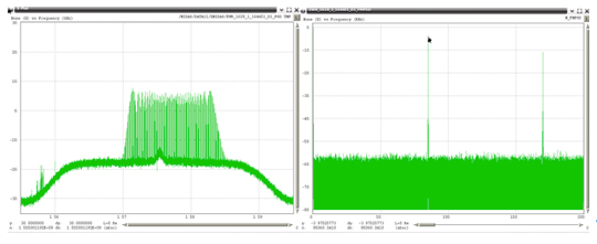
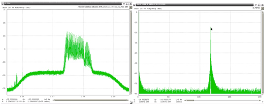
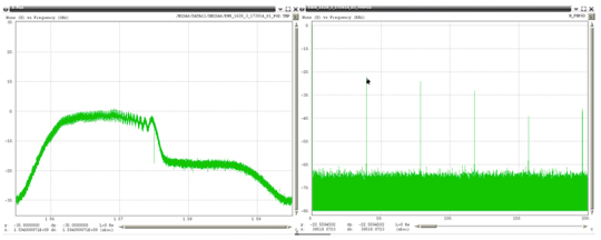
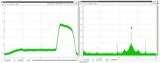
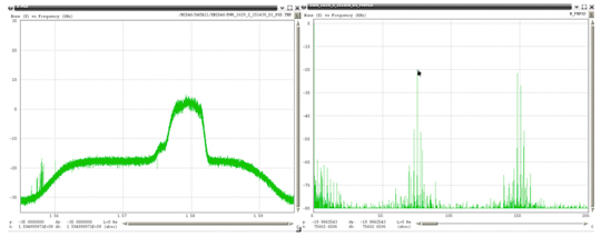
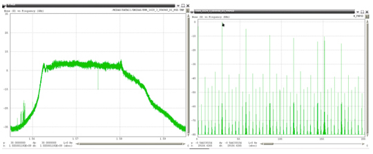
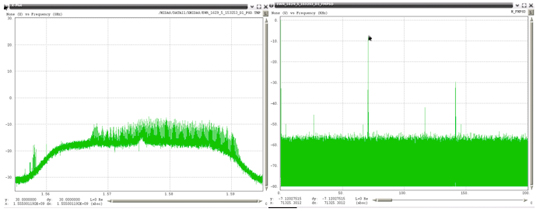
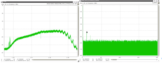
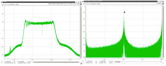
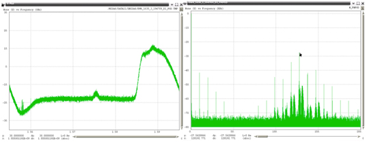
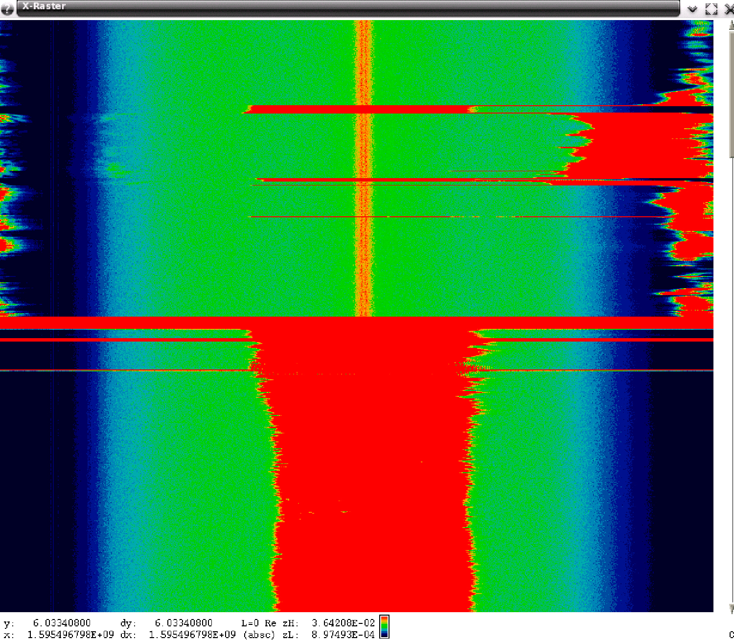
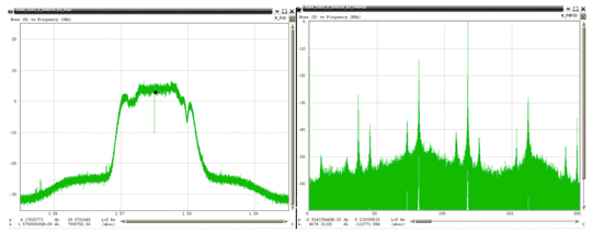
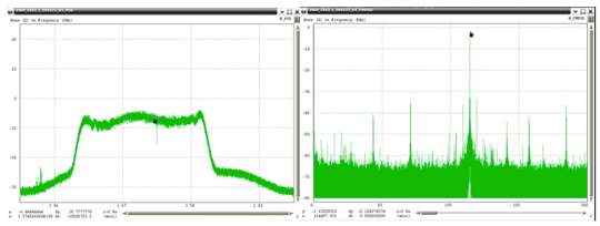
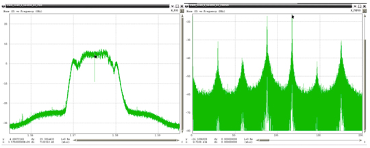
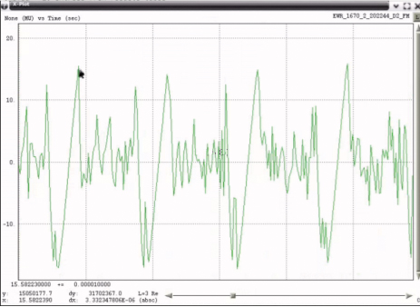
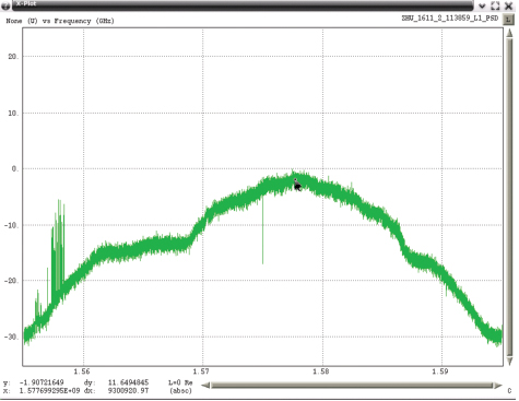
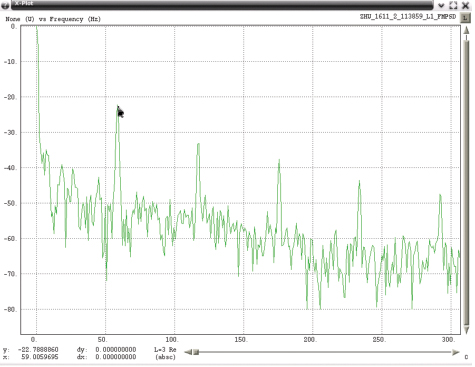
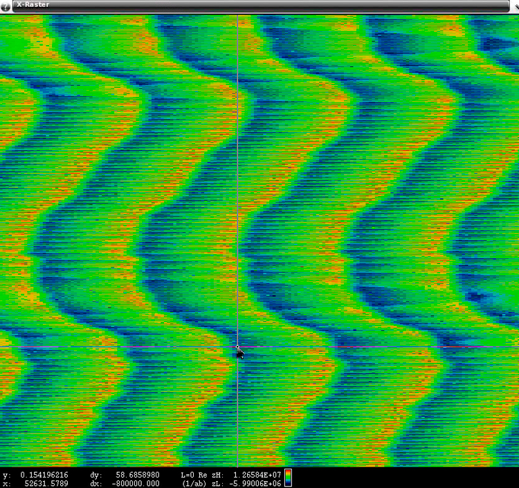
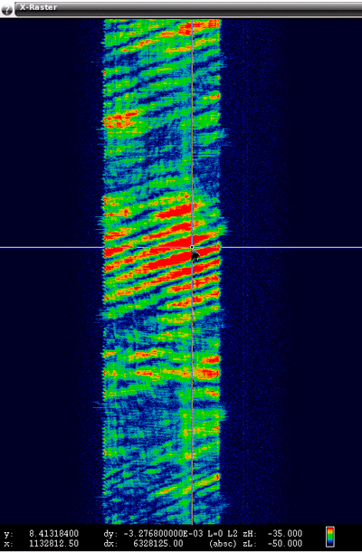
    During the Joint Interagency Field Experimentation (JIFX) event at Camp Roberts, California, in November 2014, we tested the APNT system by deploying the vehicle with GPS, UAT and DME antennas simultaneously recording data. GPS receivers on the ground were used to collect reference measurements to estimate the time of transmission of the signals from the APNT sites. All signals were recorded at an altitude of 275 meters above ground level (600 meters above sea level), at four different points roughly 800 meters apart, and the data analyzed for comparison. As expected, the UAT broadcast was noisier than the GPS signal. However, it was possible to calculate a range from the UAT data that was accurate to within 16.6 meters of the GPS reference position, well within the 30 meters error bound specified in the project specification (see FIGURE 5).

    Figure 5. UAT range deviates from GPS derived range-estimate by an average of only 16.6 meters throughout the duration of the test flight.
    Figure 5. UAT range deviates from GPS derived range-estimate by an average of only 16.6 meters throughout the duration of the test flight.

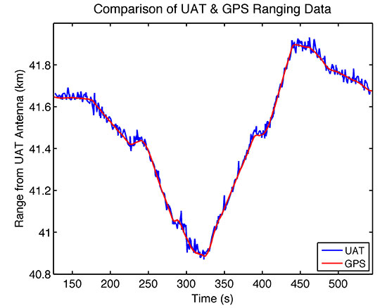
    While UAV navigation using APNT was done offline in post-processing for these tests, with planned algorithm improvements and hardware acceleration the UAT signal can be used to get real-time position information nearly as accurate as that from GPS. Thus the JAGER UAV can be navigated with comparable reliability in both GPS and GPS-denied environments.

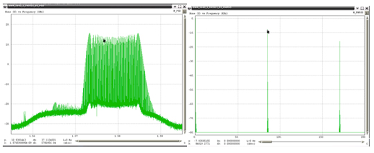
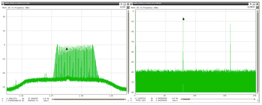
    Terrestrial APNT signals will be received at a wide range of power levels. This effect is not observed with the GPS network, as the different satellite signals are broadcast from such a great distance that any differences in received signal strength are relatively small by the time they reach Earth. For terrestrial networks, signals from transmitters close to the receiver can be many times stronger than those further away, which can result in two issues: 1) interference where one signal overwhelms another, and 2) inability to process a signal if the receiver does not have adequate dynamic range to capture strong and weak signals clearly.

    This problem was observed in our tests, as we were receiving two signals: one 13.7 kilometers (DME) and the other 43.5 kilometers (ADS-B UAT) from our test site. Calculating accurate ranging estimates from the two required determining a gain setting that had dynamic range adequate for receiving both signals clearly.

    Vehicle Performance

    During experimental testing, the vehicle itself also underwent rigorous assessment of its performance under different conditions. Due to the delicate and often expensive nature of the payloads and experiments made possible by the JAGER platform, it is essential that the vehicle perform as expected, and that there are multiple procedures in place to protect the payloads in case of vehicle failure.

    Because the open-source autopilot had never been used with such a large vehicle, we first ground-tested the craft’s flight control and stability. The vehicle was tethered and constrained to move in only one axis, and ropes were used to control its roll. While altering autopilot variables controlling roll and pitch feedback loops, we measured the vehicle’s response to impulsive disturbances and the time taken for it to right itself when upset. In this way we could tune the control gains and verify that the vehicle would be exceptionally stable during flight in even the most challenging atmospheric conditions. While we preferred to fly in the early morning hours to exploit clear air and lower winds, we did perform tests with momentary gusts of up to 7 m/s during envelope expansion flights.

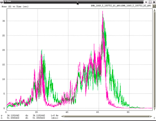
    We tested the vehicle with two accelerometers on board to measure how the rotors’ vibrations affected the rest of the craft. One accelerometer was attached to the airframe itself, while the other was secured to the payload plate. A comparison of the acceleration data recorded by the two instruments revealed that the payload plate experienced significantly less vibration than the airframe during flight, and both measurements remained well within the tolerances advised by the airframe manufacturer.

    Two crucial flight modes also were tested before payloads were flown on the vehicle. Both altitude-control mode and position-control mode were tested to ensure that they could precisely constrain respectively the vehicle’s altitude and absolute position in a range of atmospheric conditions. Results showed that in altitude control mode, the vehicle’s z-coordinate was held constant to within ± 0.5 meters. In position control mode, its x- and y-coordinates remained within ± 1.0 meters (or a single vehicle length).

    The success of the JAGER tracking mission also depends on accurate position measurements from the UAV. Operators must be confident in the vehicle’s position, so that ground forces can easily apprehend the located jammer, and also so that there is confidence in the success of safety protocols including geo-fencing, no-fly zones and minimum flight altitudes.

    In addition to the geo-fencing and flight precautions taken by the tracking algorithm, the JAGER UAV has several other safety procedures executed automatically by the autopilot. A non-catastrophic error in the flight systems or payload is transmitted to the ground station for human troubleshooting, and commands can be sent to the vehicle as to how to proceed.

    Finally, should we continue operations and allow its batteries to get sufficiently low, the vehicle will automatically return to launch site for landing and battery replacement. A catastrophic failure such as the loss of a motor will result in an immediate controlled landing. The craft can also be commanded from the ground station to land or return to launch, and can be taken over by a human pilot at any time.

    Other tests verified that the vehicle has the range and endurance to be successful when deployed in an airport setting. When fully loaded with APNT and tracking payloads, the UAV exhibited a top speed of 10 m/s, enough to cover the length of an A380-capable runway in less than 5 minutes. A 20-minute flight endurance means that even including hovering during jamming signal observations by the tracking antenna, the JAGER system can hunt easily and effectively throughout an airport-sized area. Furthermore, we continue to explore techniques to improve dash capability, including reducing the weight of the APNT payload, and we anticipate describing results of these efforts in future reports.

    Electromagnetic Interference

    Because of the payload tray’s small area (0.5 m2), electromagnetic interference (EMI) between APNT components was a significant issue during testing. The GPS and UAT receivers are extremely sensitive to interference from other sources emitting in the frequency ranges to which they are tuned. The APNT computer, by contrast, is composed of various processors, clocks, drives and power boards that emit powerful electromagnetic noise at a wide range of frequencies as a byproduct of their normal operation.

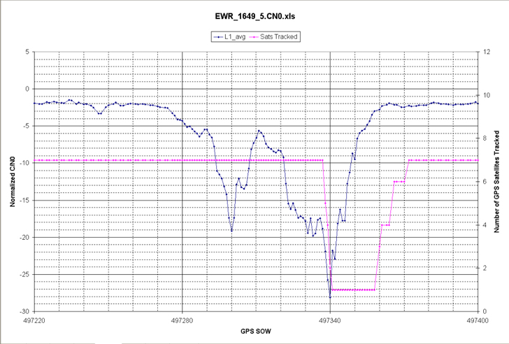
    The size and mass of the APNT computer board meant that it had to be mounted in the center of the payload tray to avoid unbalancing the UAV. That left a maximum 7 centimeters of space around the computer on which to mount the two antennas (see FIGURE 6). With no shielding, the EMI from the computer proved powerful enough to completely overwhelm the GPS, UAT and DME network signals, making navigation and position estimation using any network impossible.

    Figure 6. Diagram showing the APNT experimental payload, and the proximity of the EMI-radiating CPU to numerous antennas.
    Figure 6. Diagram showing the APNT experimental payload, and the proximity of the EMI-radiating CPU to numerous antennas.

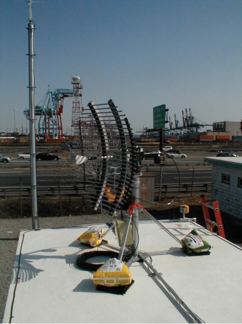
    The EMI problem was solved in three ways. Masts were used to raise the receiving antennas to a height of 19 centimeters above the payload tray, the maximum height at which a mast collapse wouldn’t cause catastrophic rotor and vehicle failure.

    The antennas also were moved around the edge of the payload tray so as to be furthest from the system components radiating at their particular frequency. Two devices that proved particularly problematic were the solid-state hard drive in the CPU and the telemetry radio antenna, which radiated EMI that interfered with the GPS and UAT frequencies respectively. This was solved by moving the telemetry antenna to the underside of the craft, and the GPS antenna to the far side of the payload plate from the hard drive. The flexible design of the payload plate described earlier ensured that the relocation and testing of components was a straightforward process.

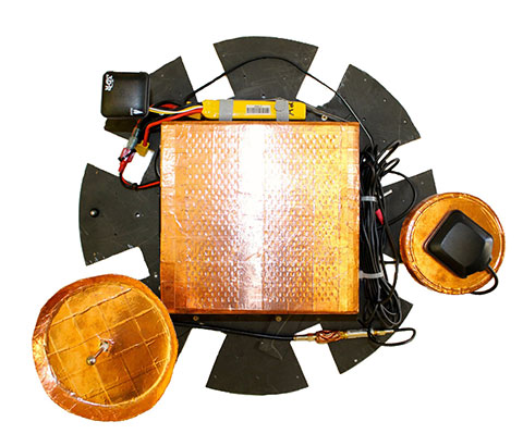
    Shielding, however, proved to be the most important factor in eliminating EMI. Custom-made copper shields were added to the two masts to shield the antennas from the computer below them while still allowing an unobstructed view of the sky (see PHOTO). We tested numerous shielding iterations, including wire meshes and aluminum and lead foils; however; all were ineffective due to the strength and wide range of EMI wavelengths emitted. Finally, the computer itself was covered in a 2-millimeter layer of copper and 1-millimeter steel sheet. This combination struck the best balance between effectiveness and weight: aluminum was light but proved ineffective at shielding, while lead was very effective at EMI shielding but was too heavy for the UAV to carry.

    The APNT payload prior to installation of the DME antenna. The copper shielding on the CPU and antennas can be clearly seen.
    The APNT payload prior to installation of the DME antenna. The copper shielding on the CPU and antennas can be clearly seen.

    Conclusions

    The development of the JAGER system contributes to U.S. preparation for a GPS jamming attack on civil aviation. While the first iteration described here is a significant improvement on previous jammer-hunting systems, future iterations of the JAGER UAV will be able to successfully navigate in a GPS-denied environment using alternative navigation signals including UAT and DME, and broadcast an accurate estimate of their position down to the ground.

    The use of an octocopter flight system gives speed, maneuverability and sensory perception that far exceed any ground-based tracking effort. A fully loaded top speed of 10 m/s and almost instantaneous direction changes allow for efficient hunting over an airport-sized area and the location of a GPS jammer to within 30 meters, within a 20-minute flight endurance.

    As the JAGER system can be entirely assembled from commercially available or open-source components and operates entirely autonomously, the system provides a low-cost, readily obtainable solution to the problem of GPS jamming. This means that it can be deployed quickly and is operable without extensive prior training.

    The integration of autopilot, APNT navigation and tracking systems also allows for comprehensive monitoring and control of the UAV from the ground. Telemetry and data links to the ground station provide real-time updates as to the craft’s position, the jammer’s believed location and the status of all systems and instruments running on the vehicle. Safety protocols implemented in the software ensure that there is no risk of collision with site buildings, vehicles or personnel.

    JAGER’s modular design gives operators extensive flexibility in situations that are capable of being successfully resolved by the system. The switching of equipment and software to allow the UAV to use GPS navigation to hunt a UAT or DME jammer, for example, could be effected in a matter of seconds.

    The JAGER system also provides a reliable test platform for any experiment that requires airborne operation. The exceptional stability of the airframe combined with extended flight time, high top speeds and pinpoint positioning lends the system to a wide variety of applications beyond jammer tracking, including network monitoring, atmospheric experiments and biological research.

    Manufacturers

    The JAGER UAV airframe is a S1000 octocopter by DJI Innovations, Shenzhen, China; the flight batteries are a 8000 mAh model by Hextronik, Dongguan, China; the autopilot hardware and GPS antenna is a Pixhawk by 3D Robotics, Inc., San Diego, California; the autopilot software is based on PX4 by Pixhawk.org. The JAGER navigation GPS is made by u-blox, and the receiver for the APNT clock is made by Trimble. The UAT hardware includes an ASR-2300 multichannel transceiver by Loctronix Corporation, Woodinville, Washington; the tracking hardware comprises a 2.4 GHz Yagi antenna from L-com, North Andover, Massachusetts; an RN-XV Wi-Fi module by Roving Networks, Chandler, Arizona; and an Odroid-U3 computer by Hardkernel Co., Gyeonggi, South Korea.


    James Spicer is pursuing concurrent bachelor’s and master’s degrees in aeronautics and astronautics at Stanford University.

    Adrien Perkins is a Ph.D. candidate in aeronautics and astronautics at the Stanford University GPS Laboratory. He received his undergraduate degree in mechanical aerospace engineering at Rutgers University.

    Louis Dressel is a graduate student at Stanford University. He received his undergraduate degree in aerospace engineering from Georgia Tech, with a minor in computer science.

    Mark James is a master’s student in aeronautics and astronautics at Stanford University.

    Yu-Hsuan Chen is a research associate at the Stanford GPS Laboratory. He received his Ph.D. in electrical engineering from National Cheng Kung University, Taiwan.

    Sherman Lo is a senior research engineer at the Stanford GPS Laboratory.

    David S. De Lorenzo is a principal research engineer at Polaris Wireless and a consulting research associate to the Stanford GPS Laboratory.

    Per Enge is a professor of aeronautics and astronautics at Stanford University, where he is the Vance D. and Arlene C. Coffman Professor in the School of Engineering. He directs the Stanford GPS Laboratory.

  • FAA: GBAS Operational at Airports Worldwide

    FAA: GBAS Operational at Airports Worldwide

    Delta Boeing 737 lands at Newark using GBAS.
    Delta Boeing 737 lands at Newark using GBAS.

    Delta Airlines made a perfect Ground-Based Augmentation System (GBAS) Landing System (GLS) landing at Liberty Newark International Airport on Feb. 18, according to the Federal Aviation Administration’s SatNavNews newsletter.

    Delta now joins United Airlines and British Airways as airlines that use the GBAS at Newark.

    More GBAS locations around the world are reaching operational status, and airline operations using GBAS are increasing as additional GLS-equipped aircraft are entering service for the various airlines. Boeing has confirmed that many of the customers who have ordered multiple 787s, 747-8s or 737s have publicly stated their intention to use the GLS capability on these aircraft.

    More than 1,000 Boeing GLS-equipped aircraft are now in use, and this number is growing by an estimated 25 airplanes per month. This estimate is based upon current production rates — one third of 737s are being equipped with the GLS option. GLS is standard on 787 and 747-8 aircraft.

    The list below provides a summary of the airlines using GBAS and the airports where GLS approaches are flown on a regular basis.

    U.S. Carriers

    • Delta Airlines – Houston, Newark
    • United Airlines – Houston, Newark

    Non-U.S. Carriers

    • Air Berlin – Bremen, Malaga
    • British Airways – Newark
    • Cathay Pacific – Houston, Sydney (plans for Newark in the future)
    • Emirates Airlines – Frankfurt, Houston, Sydney, Zurich
    • Lufthansa – Frankfurt, Houston
    • Qantas – Sydney
    • Swiss Air – Zurich
    • TUIfly – Malaga
    • Various Russian airlines (S7, Transaero, Utair, Sakhalin Energy, Gaspromavia Russia). Fifteen GBAS locations in Russia have been approved with each airline using different airports (Domodedovo, Pulkovo, Tyumen, Ostafyevo, Nogliki and others).

    The commitment to GBAS development and implementation continues to grow, according to the FAA, with plans to implement GBAS in these additional locations:

    • Dubai, United Arab Emirates
    • Chennai, India
    • Gimpo, South Korea
    • London Heathrow, United Kingdom
    • Melbourne, Australia
    • Oslo, Norway
    • Rio de Janeiro, Brazil
    • St. Helena, United Kingdom.
  • Personal Privacy Jammers: Locating Jersey PPDs Jamming GBAS Safety-of-Life Signals

    By Joseph C. Grabowski

    When jamming interfered with GPS signals at Newark Airport, a three-month effort determined that low-power, mobile personal-privacy devices were responsible. This article describes how they were found and outlines how the observable parameters of such devices encompass a wide variation in RF spectra and internal modulation.

    Personal privacy devices (PPDs) are now recognized as being responsible for causing interference to GPS receivers. However, in November of 2009, when the Local-Area Augmentation System (LAAS) installed its first Ground-Based Augmentation System (GBAS) at Newark International Airport (EWR), this fact was not known. Within the first month of its installation, anomalies in GBAS processing were correlated to the presence of radio-frequency interference (RFI). Initial efforts to determine the source of this unexpected RFI were not successful.

    The Federal Aviation Administration (FAA) had a significant interest in finding this RFI source, leading to deployment of RFI detection and location equipment by several groups. Zeta Associates temporarily installed equipment in early January 2010 that was capable of detecting and characterizing RFI but did not have emitter location capability.

    Determining that an RFI transmitter is in motion is more certain if the RFI is observed simultaneously by multiple sensors. However, analysis from hundreds of RFI events indicates that when an RFI source is in motion, observations collected by a single sensor can provide sufficient information to determine that the RFI transmitter is in motion.

    Continuing interest in understanding PPD effects on GPS receivers led to the installation of remotely accessible monitoring equipment that provides detailed characteristics of these devices. Remote access facilitates monitoring, particularly since PPDs are present for 30 to 60 seconds at a time and only a few times a day.

    Background

    The January 2010 deployment included a WAAS GPS receiver, spectrum analyzer, and a Zeta custom-developed Snapshot System, assembled from commercial off-the-shelf (COTS) equipment for conducting WAAS site-installation surveys, and capable of capturing intermittent short-duration RFI events. It consists of a tuneable receiver (10 MHz to 3 GHz) whose RF front end spans 25 MHz that is digitized at a sample rate of 56 MHz, with storage capacity sufficient for up to 80 minutes. Once captured, the time-series data can be analyzed in many different ways. Possible analysis techniques include examination of the raw time samples, generation of spectral plots, or demodulation of the RFI signal. Each approach can lead to a better understanding of the underlying interference signal. If digital data is present and can be demodulated, it might be possible to associate the demodulated bits with a known transmitter.

    Data can be captured manually or programmatically using a trigger determined by an algorithm that monitors WAAS GPS receiver automatic gain control (AGC) logs. The AGC function within a WAAS receiver has a well-behaved response for normal Gaussian noise RF environments. When RFI is present, the AGC exhibits atypical responses that then trigger the Snapshot System. As WAAS receivers utilize both L1 and L2, and each RF path has its own AGC, it is possible to detect the presence of potential RFI at either L1 or L2.

    The Snapshot System RF input for this deployment was from a PCTEL antenna identical to those used at WAAS reference sites. This antenna incorporates a triplexer that provides three separate 40 MHz passbands each centered on L1, L2, and L5, with approximately 50 dB of gain. This antenna was located approximately one mile north of the four LAAS antennas within Port Authority of New York and New Jersey (PANYNJ) Building 80.

    Within the first hour of being deployed on January 20, 2010 the Snapshot System had detected and captured one RFI event in the GPS L1 band. After one day, the Snapshot System had detected and captured more than 25 separate instances of RFI within the GPS L1 band. Most RFI events were narrowband (10s of kHz bandwidth) and short duration (no more than 3 seconds).

    However, there also were five RFI events that spanned more than 15 MHz across L1 (Figure 1) were present as long as 20 seconds and at a power level as much as 25 dB above the receive antenna’s noise floor. Some of these RFI events were strong enough to reduce a WAAS G-II receiver C/N0 by as much as 20 dB and thereby resulted in loss of tracking for lower-elevation GPS satellites. Higher-elevation GPS satellites were able to continue tracking throughout these events but at a lower C/N0. The wideband RFI events were also detected by the SLS 4000 GBAS monitor and coincided with tracking problems in the LAAS GBAS receivers.

    Credit: Joseph C. Grabowski
    FIGURE 1. EWR wideband RFI.

    Two of the captured broadband RFI events were demodulated and analyzed. The underlying linear frequency modulation (FM) signal swept over more than 15 MHz in less than 1 millisecond (Figure 2).

    Credit: Joseph C. Grabowski
    FIGURE 2. FM demodulated wideband RFI.

    At that time, it was not known if the source of the RFI was stationary or moving, whether it was unintentional (emanating from a licensed transmitter but with malfunctioning electronics), inadvertent (equipment normally used for test purposes and capable of operating in the GPS band but accidentally left on), or intentional (purposeful jamming of GPS).

    Since the RFI was observed by GPS receivers separated by 1,700 meters, a search was undertaken to identify any other GPS receivers in the vicinity of EWR. One National Geodetic Survey (NGS) continuously operating reference site (CORS) NJI2 is located near EWR about 4,500 meters northwest from Building 80. Analysis of data from NJI2 during the same time periods that RFI was detected by the WAAS and LAAS receivers did not contain any indication of RFI, and therefore suggested that the source of RFI was more localized to EWR.

    The Snapshot System remained in place for approximately two weeks before moving to another location. Collected data was analyzed, showing that wideband RFI was associated with significant degradation to both the WAAS and LAAS receivers. Additional characteristics noted the RFI was intermittent, lasting typically 30 seconds but no more than 60 seconds, was observed more often Monday through Friday, and most frequently around 8 a.m. local time.

    Locating The RFI

    Figure 3 shows a Google map of EWR with blue dots indicating the location of the four LAAS antennas, a green dot for Building 80, and a yellow dot for the GBAS shelter. EWR is adjacent to the New Jersey Turnpike (NJT), which has seven southbound and seven northbound lanes of traffic.

    Credit: Joseph C. Grabowski
    FIGURE 3 Google map of EWR.

    Since the Snaphsot System did not include location capability, other teams with direction-finding equipment, including beam-forming antennas, travelled to EWR to try to locate the RFI source. These teams were on site at various times from February to March. However, those efforts did not provide sufficiently reliable information to reduce the search area. By mid-March, the search area remained identical to that of January.

    Zeta then deployed two WAAS G-II receivers separated by considerable distance (1,722 meters) to monitor for RFI, and analyze each receiver’s response only when RFI sufficient to significantly degrade GPS reception was detected. One receiver was located within Building 80, and the second receiver within the GBAS shelter near the LAAS antennas. This configuration was designed to determine degradation relative to each reference receiver and thereby establish probable search areas for the RFI emitter. The Zeta equipment also incorporated a rotating directional antenna (at the GBAS shelter shown in Figure 4) that was commanded to rotate only when significant RFI was detected.

    Credit: Joseph C. Grabowski
    FIGURE 4A. Antennas on roof of GBAS shelter.
    Credit: Joseph C. Grabowski
    FIGURE 4B. Antennas on roof of GBAS shelter.

    The expectation was that RFI would be detected simultaneously by both GPS receivers, and that the relative degradation in normalized C/ N0 would provide an indication as to which location lay in closer proximity to the RFI source. The rotating high-gain directional antenna would then indicate a reduced probable search area consistent with the relative degradation between the two receivers. At the time this equipment was deployed, it was still thought that the RFI was most likely stationary and high-power. However, the measurement results were quite different than expected. Subsequent data analysis from this equipment revealed that the RFI was low-power and moving, specifically moving along the NJT.

    The Zeta equipment was deployed on March 19, 2010, and remained in place while operating automatically. On March 25, data collected during the previous week were analyzed. During this 1-week collection there were 11 instances when both receivers detected wideband RFI events and one antenna rotation even partially tracked one wideband RFI emitter. Such data was indicative of a non-stationary emitter, a finding that was quite significant. Based on data from the two receivers, the apparent velocity of the RFI emitters ranged between 45 miles per hour (mph) to 72 mph. Initial analysis of antenna-rotation data also indicated the RFI source was east of the GBAS shelter and moving south on the NJT.

    Understanding the importance of degradations from both receivers was crucial in determining that the RFI has attributes of transmitting at low power and is moving. Had a single stationary RFI emitter been responsible for these observations, the degradations measured at each receiver would have occurred at essentially the same time, not 50 to 80 seconds apart. A high-power moving RFI emitter would also have produced degradations at both receivers at the same time, and since that was not observed, the conclusion was that the RFI emitter was relatively low in output power. Low-power RFI emitters will cause significant degradation to GPS receivers only when they are in close proximity to them, on the order of hundreds of meters.

    Receiver data logs were processed specifically for degradation in normalized C/N0. Normalized C/N0 was only computed for those satellites above 20 degrees, and all of those results were averaged together. Prior knowledge regarding WAAS PCTEL antennas has established an expected C/N0 versus satellite elevation that is accurate to approximately ±1 dB with a nominal mean of 0 dB. This normalized C/N0 represents an average of all satellites in view. However, individual satellite signal strength can vary greater than ± 1 dB. Significant deviations of more than –3 dB are indicative of strong RFI within the GPS processing band. Normalized C/N0 was plotted for each day that data was collected, followed by expanding those time periods where significant degradation was present.

    Figure 5 shows data of the first evidence of a low-power moving PPD. Data for Building 80 receiver is in blue and data from the GBAS shelter receiver in pink. Since Building 80 is north of the GBAS shelter, when degradations occurred first at Building 80, this implies that the RFI emitter is moving from north to south. Similarly, when degradations were first seen at the GBAS shelter, the RFI emitter was moving from south to north. This plot uses major time grids of 60 seconds and minor grids of 10 seconds.

    Credit: Joseph C. Grabowski
    FIGURE 5. Normalized C/N0 observed at Building 80 and GBAS shelter.

    The double separate degradations observed by the Building 80 receiver have only been observed from monitoring equipment located at that building, and have since been associated with travel paths of PPDs on the nearby highways. Both GPS receiver and spectral data contain this same characteristic. This characteristic is due to the fact that vehicles traveling south on the NJT have clear line of sight to the roof of Building 80 (shown by Figure 6) before they travel under Interstate 78, after which they pass next to Building 80. During the time that they are under Interstate 78, their transmissions are blocked in the direction of the roof of Building 80.

    Credit: Joseph C. Grabowski
    FIGURE 6A. View of NJT near Building 80.
    Credit: Joseph C. Grabowski
    FIGURE 6B. View of NJT near Building 80.

    Spectral data as observed by the 4-foot reflector is shown in Figure 7. Figure 8 shows spectral maximum data as collected by the 4-foot linearly polarized reflector along with additional information.

    Credit: Joseph C. Grabowski
    FIGURE 7. Wideband RFI observed by 4-foot reflector (click to enlarge.)
    Credit: Joseph C. Grabowski
    FIGURE 8A. Pink represents spectral maximum data as observed through the reflector, green represents the azimuth of that antenna, and blue the reported degradation of the GBAS shelter receiver.
    Credit: Joseph C. Grabowski
    FIGURE 8B. Pink represents spectral maximum data as observed through the reflector, green represents the azimuth of that antenna, and blue the reported degradation of the GBAS shelter receiver.

    When the GBAS shelter receiver at first detected RFI, the reflector began rotating from an azimuth of 0 degrees in a clockwise direction. At the same time, a spectrum analyzer began capturing spectra at a rate of 3 per second. The first spectral maximum was observed at an azimuth of 30 degrees, a direction in which the antenna was pointed towards the NJT, to a location approximately 900 meters away from the GBAS shelter. The next time spectra were at high levels occurred for azimuths between 145 to 195 degrees, or southeast of the GBAS shelter. The approach of using a rotating antenna was originally intended to provide a direction towards a stationary source and not to track a moving emitter. However, it appears that to some extent, the rotating antenna in fact did track a moving emitter from north to south.

    On the afternoon of the day these results were communicated to the FAA lead for the EWR RFI investigation, all search activities were shifted to the NJT and away from the airport operating area. Just south of the GBAS shelter there is an official-use overpass that straddles the NJT. All detection equipment was positioned onto the overpass, under the hypothesis that the RFI was emanating from vehicles traveling the NJT. Evidence substantiating this initial finding was found within a day, and approximately one month later a concerted effort was undertaken to identify and stop a single vehicle that was using a PPD.

    The Zeta equipment remained in place for many months and continued to provide additional evidence of PPD characteristics. Early in the investigation it was hoped that only a few PPDs had been responsible, but as more data was collected it became evident that many different types of PPDs were traveling along the NJT past EWR.

    Modeling PPD Effect

    Once it was realized that the RFI was from low power moving emitters, a simple model was used to predict their degradation effect on WAAS GPS receivers. The model shown in Figure 9 was used for the purpose of computing distance between the RFI emitter and a WAAS antenna and to then compute the additional level of interference noise power that the WAAS antenna would receive. Here, the WAAS PCTEL antenna is located 50 meters from a road that is 2000 meters long and straight and has an RFI emitter transmitting +25 dBm, moving at 32.5 meters per second (72.5 mph) and with clear line of sight to the WAAS antenna.

    FIGURE 9. Simple model of moving emitter.
    FIGURE 9. Simple model of moving emitter.
    Credit: Joseph C. Grabowski
    FIGURE 10. Model of normalized C/No due to a PPD.

    With these assumptions it is a simple matter to compute the additional noise power at the WAAS antenna. Non-coherent summation of the RFI noise and inherent system noise was used to compute the total noise power and therefore the additional degradation in C/N0. The resulting predicted degradation was overlaid on one of the actual RFI events and is shown as a green line in Figure 10. The predicted degradation closely resembles actual event data logged by receivers.

    The shape of degradation in normalized C/N0 versus time has been observed in nearly all of the EWR RFI events that have been analyzed. The magnitude of degradation depends on the power of the RFI and its proximity to the GPS antenna, while its time duration depends on the velocity of the vehicle carrying the PPD. The shape is directly related to the distance versus time between the vehicle and the WAAS antenna. Faster/slower moving vehicles with PPDs will simply shrink/stretch the time scale.  Curved roadways would have different shapes that could also be readily predicted.

    CORS data was revisited after realizing that PPDs were traveling the NJT. Specifically, two CORS sites CTDA (70 meters from Interstate 95) and NJDY (380 meters from Interstate 95) were identified. Data from those two sites were analyzed for a couple of weekdays. Possible evidence of PPDs was found within that data. Reported Signal to Noise Ratio (SNR) from CTDA and NJDY contained variations similar to those observed by GPS receivers at EWR during times when PPD induced RFI has been detected.

    Continued RFI Monitoring

    The LAAS program desired continued monitoring of RFI from PPDs near EWR, including estimates of their effective isotropic radiated power (EIRP). Additional equipment was assembled to provide this capability and installed on March 3, 2011. This monitoring equipment is located within the GBAS shelter at EWR and comprises several COTS components that incorporate improvements beyond the first Snapshot System used at EWR. Improvements include an upgraded Snapshot System (Figure 11), an RHCP directional antenna, and a wireless modem that provides remote access to the monitoring equipment.

    Credit: Joseph C. Grabowski
    Figure 11A. Snapshot System ICEPOD6-M5.
    Credit: Joseph C. Grabowski
    FIGURE 11B. Snapshot System laptop.

    Remote access makes it possible to analyze captured RFI data from any computer connected to the Internet, and to modify software if necessary. The new equipment configuration, specifically the use of an AEL AST 1507AA RHCP antenna, was chosen with the explicit purpose of establishing more accuracy in estimated EIRP.

    Analysis of data collected during 2010 indicated three significant sources of error in estimating EIRP; Free Space Loss (FSL) from not knowing the exact position of the PPD on the NJT, polarization mismatch loss between the PPD antenna and the receive antenna, and the effects due to transmission from within a vehicle. Differences in FSL loss between the closest southbound lane on the NJT and the most distant northbound lane is on the order of 11 dB. If it is known that the PPD is traveling south, the difference in FSL between the nearest to farthest southbound lanes is less but still about 6 dB. FSL differences for northbound lanes are smaller, on the order of 3 dB. Knowing the direction of travel reduces this uncertainty but does not eliminate it. The WAAS PCTEL antenna is RHCP, but at the horizon has an axial ratio of approximately 5 dB. Many PPDs appear to be using quarter wavelength dipole antenna that are mounted with a rotatable connector. Assuming all PPD antennas are linearly polarized, there would then be an uncertainty of about 5 dB when using data observed by the WAAS PCTEL antenna. The AEL antenna has an axial ratio of 0.2 dB at L1 and significantly reduces uncertainty of polarization mismatch loss. Even though the AEL antenna has a 3 dB mismatch loss, that loss has an uncertainty of 0.2 dB for any orientation of the PPD antenna. The PCTEL antenna has a symmetric gain response relative to the NJT. The AEL antenna was pointed to the north intentionally so that observed RFI power will be stronger when a PPD is north of the GBAS shelter. Simultaneous capture of real time samples from both antennas by the ICEPOD6-M5 provides an indication of the direction in which the PPD is traveling. The third uncertainty comes from the effects of the PPD being located within a vehicle. Vehicular effects on the PPD transmitters were not accounted for due to difficulty in using a simple model. Aloi [1] has measured vehicular effects of quarter wavelength dipole antenna (typically used by PPDs) and has previously published [1] [2] on the effect of vehicles on GPS signals. His most recent findings have not yet been published but indicate that the type of vehicle, the location of a dipole antenna within it, and the position outside of the vehicle from which power is being measured, can lead to significant variation (10 to 15 dB) of the observable power. Consequently, the reported EIRP estimates from the Snapshot System have been referenced to a point just outside the vehicle and do not attempt to account for vehicular effects.

    Figure 12 shows a block diagram of the current monitoring equipment. The PCTEL antenna along with the WAAS G-II receiver is used for monitoring GPS signals. WAAS G-II receiver logs are monitored continuously and saved to disk, but snapshots are only taken if the RFI algorithms indicate that RFI is present. A snapshot will be taken if any of three tests (based on AGC, normalized C/N0, or spectral power) are exceeded. Narrowband RFI tends to most impact the AGC response, while wideband RFI tends to trigger the normalized C/N0 metric. Since the Snapshot System is also continuously monitoring the RF spectra from both antennas, an additional test checks if there are significant spectra changes.

    Credit: Joseph C. Grabowski
    FIGURE 12. Current Snapshot monitoring block diagram.

    The AEL antenna is connected to a filter/low noise amplifier (LNA) (Delta Microwave L5995) identical to those within the PCTEL antenna, before it is connected to one of the two L-band tuners (900 to 2200 MHz) of the ICE-Online ICEPOD6-M5, which includes 1 TB of long-term storage and 8 GB of high-speed RAM and is capable of sustained data transfers of as high as 400 MB/s between the L-band tuners and disk. Sample rates and RF filtering are programmable and have been set to use a complex sample rate of 40 MSPS and an RF bandwidth of 30 MHz. When RFI is present, data transfers are 320 MB/s. The internal 1 TB disk can store approximately 100 minutes of RFI. Software parameters limit RFI data capture for any single event to no more than 90 seconds. Implementation of a circular buffer within the high-speed RAM (8 seconds for each L-band tuner path) allows continuous capture of RF data while waiting for a trigger indicating that RFI is present. To reduce false alarms, RFI must be present for at least 4 seconds before data is captured. However, no RFI data is lost, because the circular buffer is longer than 4 seconds. RFI data captures typically contain 3 seconds of data at the beginning, with no RFI, and therefore make it possible to observe the onset of the RFI.

    The new equipment has captured hundreds of RFI events, spanning a wide range in bandwidth (7 MHz to an estimated 150 MHz), chirp rate (9 kHz to 170 kHz), and power levels (–10 dBm to as much as +20 dBm). Accurately estimating EIRP of moving emitters is a challenge and requires detailed knowledge of the characteristics of all components used in generating the estimate. Furthermore, distance to the RFI source can only be inferred, since its movement precludes exact measurement, and consequently there will always be some uncertainty in any reported EIRP. However, even with these qualifications, there is evidence from Snapshot System data that some of the RFI sources are transmitting at power levels as much as +20 dBm.

    Modeling Antenna Responses

    The use and orientation of the two antennas was chosen to determine the direction that PPDs are traveling and thereby reduce some of the uncertainty with respect to their exact location. Figure 13 shows the direction (58 degrees) in which the AEL antenna is pointed.

    Credit: Joseph C. Grabowski
    FIGURE 13. Pointing direction of the AEL antenna.

    The combination of its beam width (70 degrees) and axial ratio (0.2 dB) results in a nearly uniform gain across all lanes north of the GBAS shelter. Although FSL still depends on the exact location of the PPD, this approach does reduce many of the uncertainties associated with estimating EIRP. Since the PCTEL antenna has an omnidirectional pattern it will have a symmetrical response.

    To determine the time that maximum PPD power would be observed by each antenna, a model was used that assumed the PPD was transmitting at constant power, with fixed polarization, travelling at a constant velocity, and there were no obstacles between the transmitter and each antenna. FSL was calculated for each second of travel and used to determine the magnitude of RFI power that would be received. This value was then used to calculate a nominal Interference to Signal (I/S) relative to the GPS signal. The distance between each antenna and each of the travel lanes on the NJT were also used. The intent of this model was to understand how I/S would vary with time for each of the NJT travel lanes. Figure 14 shows the predicted I/S for the PCTEL antenna and Figure 15 for the AEL antenna. In each of these plots red, yellow and orange represent 3 of the 7 south bound travel lanes and green, blue and purple represent 3 of the 7 north bound travel lanes. A time of 0 was used for the time when the PPD is nearest physically to the GBAS shelter. A nominal velocity of 30 meters/second (67 MPH) was used for the PPD and I/S was computed for 30 seconds before and after its closest approach (± 900 meters north and south of the GBAS shelter). If the PPD travels slower than 30 m/s then the following curves would be wider for the same times. Similarly, if the PPD travels faster, these same curves would be narrower.

    Credit: Joseph C. Grabowski
    FIGURE 14. Predicted I/S for PCTEL antenna (click to enlarge.)
    Credit: Joseph C. Grabowski
    FIGURE 15. Predicted I/S for AEL AST-1507AA (click to enlarge.)

    Modeling of the AEL antenna took into account its pattern and orientation. It has less gain towards the south, and consequently observed power from a PPD located south of the GBAS shelter is much less. A southbound PPD will initially be within the main beam of the AEL antenna; therefore the expected interference to signal ratio (I/S) will gradually increase until it passes to the south of the GBAS shelter. Similarly, a northbound PPD will not exhibit significant I/S until north of the GBAS shelter. Figure 15 indicates that the maximum I/S occurs within 2 seconds of the point where the PPD is closest to the GBAS shelter. Typical GPS receivers can tolerate an I/S of 30 dB for CW type signals.

    Processed RFI data does display some of these characteristics but with some important differences. PPD power was measured once every millisecond using Snapshot System data and total power within the bandwidth of that PPD was calculated. Total power from both the PCTEL (green) and AEL (pink) antennas were then plotted together with one example for a southbound PPD in Figure 16 and a northbound PPD in Figure 17.

    Credit: Joseph C. Grabowski
    FIGURE 16. RFI Power of southbound PPD (click to enlarge.)

    Credit: Joseph C. Grabowski
    FIGURE 17. RFI Power of northbound PPD (click to enlarge.)

    Although the envelope of the measured average power tends to have the shape that modeling predicts, there are significant variations over short periods of time. Figure 18 expands a portion of one example and indicates that RFI power varied by more than 17 dB in 0.2 seconds. Examination of spectral data for time intervals of less than one second frequently contains significant changes in observable power. Swept CW from PPDs should exhibit relatively flat RF spectral power, but typical observed spectra include sloping across the band and notches. Possible explanations for these observations include: blockage and diffraction from other vehicles near the one containing the PPD, multipath from other vehicles on the NJT, and the effect of transmitting from within a vehicle. Although some of the snapshot captures exhibit smooth power variation similar to predicted, the vast majority of the hundreds of snapshots exhibit significant variations in power.

    Credit: Joseph C. Grabowski
    FIGURE 18. RFI Power of southbound PPD (expanded).

    Examples of Observed PPDs

    The variety of PPDs observed by the updated EWR monitoring equipment has been surprising. Within its first month of operation, more than 40 PPDs were observed with no less than 19 from unique and different PPD transmitters. Classification of PPD transmitters is based on the combination of RF spectra and the spectrum of the FM demodulated data. Although the observed PPD transmitters use a linearly swept FM sawtooth, most contain deviations from a pure linear sweep. Figure 19 shows examples of FM demodulated time series. Rather than attempting to uniquely describe the attributes of each type of deviation, it is simpler to compute the spectrum of the FM demodulated data. The fundamental frequencies of chirp rates that have been observed have spanned 9 kHz to 170 kHz. Figure 20 shows a histogram of chirp rates observed near EWR and indicates that the most frequent rates have been 9, 26, 29, 72, 85, 118, 123, 159 and 170 kHz.


    FIGURE 20. Histogram of EWR PPD chirp rates.Credit: Joseph C. Grabowski
    FIGURE 20. Histogram of EWR PPD chirp rates.

    Examples of the 19 unique PPDs (detected within one month) are shown in Figure 22 through Figure 40, with the RF spectrum shown on the left, and the spectrum of the FM demodulated shown on the right. In each of these plots the scaling for the RF spectra is identical, spanning 40 MHz centered on 1575 MHz with a vertical scale using 10 dB per grid. All of the FM demodulated spectra use a horizontal axis that spans 0 to 200 kHz. For references purposes Figure 21 shows the RF spectra when no RFI is present.

    Some of these PPDs were transmitting at power levels (observed by the PCTEL antenna) as much as 40 dB above the LNA noise floor. Most spectra were not centered symmetrically about L1 with some completely outside the mainlobe of the GPS C/A code. A few were transmitting outside the programmed 40 MHz bandwidth of the Snapshot System (1555 to 1595 MHz). For those PPDs transmitting outside this band, estimates were made of the upper or lower frequencies using the linear slope of the FM demodulated data, and then extrapolating that slope based on the chirp interval.

    Some of the FM demodulated spectra contain a single spectral line that indicates the waveform modulating the RF has a very linear sweep. Most contain additional harmonic lines about the major component and a few appear to have bandwidth about their main spectral component. The current hypothesis is that many of these devices are poorly shielded and that the internal oscillator used to modulate the RF is affected by other nearby signals that are then appearing at the RF output. Some of the possible sources could be circuits that are within the device itself but there is some evidence that a few of these devices are susceptible to energy external to the PPD. A Snapshot System located near Houston International Airport (ZHU) has captured data from PPDs that contain strong components at 58.7 Hz in addition to its linearly swept 97 kHz waveform. Since this frequency is sufficiently different from utility AC power sources (60 ± 0.03 Hz), it has been hypothesized the vehicle carrying that PPD, also has a power inverter. Most power inverters are specified to provide a frequency output of 60 ± 3 Hz. Figure 32 shows a spectral notch that was present at that single frequency throughout the complete capture and suggests that that particular device may have had an impedance matching problem in its transmission path.

    FIGURE 21. Spectra with No RFI Observed by PCTEL (click to enlarge). Credit: Joseph C. Grabowski
    FIGURE 21. Spectra with No RFI Observed by PCTEL (click to enlarge).
    FIGURE 2. 1570 to 1583 MHz, Chirp 117.35 kHz.  Credit: Joseph C. Grabowski
    FIGURE 22. 1570 to 1583 MHz, Chirp 117.35 kHz.
    FIGURE 23. 1556 to 1583 MHz, Chirp 28.43 kHz.  Credit: Joseph C. Grabowski
    FIGURE 23. 1556 to 1583 MHz, Chirp 28.43 kHz.
    FIGURE 24. 1565 to 1578 MHz, Chirp 123.13 kHz.  Credit: Joseph C. Grabowski
    FIGURE 24. 1565 to 1578 MHz, Chirp 123.13 kHz.
     FIGURE 25 1568 to 1583 MHz, Chirp 111.08 kHz.  Credit: Joseph C. Grabowski
    FIGURE 25. 1568 to 1583 MHz, Chirp 111.08 kHz.
    FIGURE 26. 1578 to 1589 MHz, Chirp 118.07 kHz.  Credit: Joseph C. Grabowski
    FIGURE 26. 1578 to 1589 MHz, Chirp 118.07 kHz.
     FIGURE 27. 1568 to 1584 MHz, Chirp 8.92 kHz.  Credit: Joseph C. Grabowski
    FIGURE 27. 1568 to 1584 MHz, Chirp 8.92 kHz.
    FIGURE 28. 1572 to 1584 MHz, Chirp 121.93 kHz. Credit: Joseph C. Grabowski
    FIGURE 28. 1572 to 1584 MHz, Chirp 121.93 kHz.
     FIGURE 29. 1557 to 1622 MHz, Chirp 36.14 kHz.  Credit: Joseph C. Grabowski
    FIGURE 29. 1557 to 1622 MHz, Chirp 36.14 kHz.
     FIGURE 30. 1568 to 1582 MHz, Chirp 11.08 kHz.  Credit: Joseph C. Grabowski
    FIGURE 30. 1568 to 1582 MHz, Chirp 11.08 kHz.
     FIGURE 31. 1570 to 1585 MHz, Chirp 85.06 kHz.  Credit: Joseph C. Grabowski
    FIGURE 31. 1570 to 1585 MHz, Chirp 85.06 kHz.
     FIGURE 32. 1572 to 1582 MHz, Chirp 118.07 kHz.  Credit: Joseph C. Grabowski
    FIGURE 32. 1572 to 1582 MHz, Chirp 118.07 kHz.
     FIGURE 33. 1529 to 1577 MHz, Chirp 39.52 kHz.  Credit: Joseph C. Grabowski
    FIGURE 33. 1529 to 1577 MHz, Chirp 39.52 kHz.
     FIGURE 34. 1578 to 1594 MHz, Chirp 131.33 kHz.  Credit: Joseph C. Grabowski
    FIGURE 34. 1578 to 1594 MHz, Chirp 131.33 kHz.
     FIGURE 35. 1575 to 1582 MHz, Chirp 75.66 kHz.  Credit: Joseph C. Grabowski
    FIGURE 35. 1575 to 1582 MHz, Chirp 75.66 kHz.
     FIGURE 36. 1561 to 1586 MHz, Chirp 29.16 kHz.   Credit: Joseph C. Grabowski
    FIGURE 36. 1561 to 1586 MHz, Chirp 29.16 kHz.
      FIGURE 37. 1568 to 1592 MHz, Chirp 71.33 kHz.  Credit: Joseph C. Grabowski
    FIGURE 37. 1568 to 1592 MHz, Chirp 71.33 kHz.
     FIGURE 38. 1560 to 1595 MHz, Chirp 9.88 kHz.  Credit: Joseph C. Grabowski
    FIGURE 38. 1560 to 1595 MHz, Chirp 9.88 kHz.
     FIGURE 39. 1564 to 1582 MHz, Chirp 100.48 kHz.  Credit: Joseph C. Grabowski
    FIGURE 39. 1564 to 1582 MHz, Chirp 100.48 kHz.
     FIGURE 40. 1584 to 1599 MHz, Chirp 128.20 kHz.  Credit: Joseph C. Grabowski
    FIGURE 40. 1584 to 1599 MHz, Chirp 128.20 kHz.

    A few snapshots have also provided evidence that some of the PPDs are erratic and probably not functioning as their manufacturer intended. Figure 41 contains a raster of 6 seconds of spectral data that shows a PPD whose output was meant to be between 1560 and 1580 MHz but for short periods of time was transmitting at frequencies above 1580.

     FIGURE 41. Spectral Raster, PPD with Unstable Output.  Credit: Joseph C. Grabowski
    FIGURE 41. Spectral Raster, PPD with Unstable Output.

    Remarks on Additional PPDs

    Since April 2011 the Snapshot System has captured many additional and different PPDs. No effort has been carried out to catalog all of the different types that have been observed but the following describes interesting and notable PPDs.

    Figure 42 shows characteristics of a PPD that has had estimated EIRP approaching +20 dBm, to a point just outside the vehicle, and has also been associated with GPS receiver C/N0 degradation of more than -27 dB, strong enough to cause the WAAS receiver, located at the GBAS shelter, to lose lock on all GPS satellites for a short period of time.

     FIGURE 42. 1568 to 1582 MHz, Chirp 118 kHz .  Credit: Joseph C. Grabowski
    FIGURE 42. 1568 to 1582 MHz, Chirp 118 kHz

    Figure 43 shows a PPD that is one of the most frequently observed PPDs but that has not been associated with any significant degradation to the GPS receivers.  Estimated EIRP for these PPDs has been on the order of no more than +10 dBm. One device with similar characteristics was procured and its measured power at the antenna output port was no more than +14 dBm. Marketing information on the internet for that PPD specified its output power as +25 dBm.

     FIGURE 43. 1572 to 1589 MHz, Chirp 85 kHz.  Credit: Joseph C. Grabowski
    FIGURE 43. 1572 to 1589 MHz, Chirp 85 kHz.

    Figure 44 shows a PPD that is transmitting at both L1 and L2. The EWR Snapshot System has been configured to only capture snapshot data at L1 due to the fact that LAAS only uses L1. However, the WAAS receiver used to monitor for RFI is a dual frequency receiver that on occasion has indicated simultaneous RFI at both L1 and L2. Even though the EWR Snapshot System has not captured data at L2, the simultaneous presence of both L1 and L2 RFI, provides strong circumstantial evidence that this RFI source was transmitting on both frequencies. A Snapshot System monitoring the WAAS Reference Station (WRS) at Leesburg Virginia has captured simultaneous L1 and L2 RFI events. Demodulation of that data indicated the two RF outputs had similar modulation but the demodulated data was not coherent. Therefore, that PPD was probably using individual, but similar waveform generators, for each RF output.

     FIGURE 44. 1562 to 1583 MHz, Chirp 114 kHz. Credit: Joseph C. Grabowski
    FIGURE 44. 1562 to 1583 MHz, Chirp 114 kHz.

    Almost all PPDs have been observed individually. However, there have been at least three times in the last two years when two unique PPDs have been observed within 60 seconds of each other. Figure 45 plots normalized degradation in C/N0 while Figure 46 plots snapshot measured power for the same RFI event. Analysis of snapshot data for each of the times that had strong RFI power are shown in Figure 47 and Figure 48 and confirmed that there were in fact two unique PPDs observed approximately 40 seconds apart. Both were traveling south on the NJT and approximately 1200 meters apart.

     FIGURE 45. Normalized C/N0 August 19, 2011.  Credit: Joseph C. Grabowski
    FIGURE 45. Normalized C/N0 August 19, 2011
     FIGURE 46. Snapshot Power August 19, 2011.  Credit: Joseph C. Grabowski
    FIGURE 46. Snapshot Power August 19, 2011.
     FIGURE 47. C/N0 -19.0 dB, Chirp Rate 78.97 kHz.  Credit: Joseph C. Grabowski
    FIGURE 47. C/N0 -19.0 dB, Chirp Rate 78.97 kHz.
     FIGURE 48. C/No -28.0 dB, Chirp Rate 117.24 kHz. Credit: Joseph C. Grabowski
    FIGURE 48. C/No -28.0 dB, Chirp Rate 117.24 kHz.

    Most of the observed RFI events last for no more than 50 seconds although a few that lasted much longer have been correlated with slow traffic on the NJT. Figure 49 is from June of 2010, before the updated monitoring equipment was in place, and displays normalized degradation of C/N0. The time duration for which this RFI was observed was more than 3 minutes and was during a time when traffic was ‘slow’ on the NJT.

     FIGURE 49. June 9, 2010, PPD, Estimated Velocity 10 m/s. Credit: Joseph C. Grabowski
    FIGURE 49. June 9, 2010, PPD, Estimated Velocity 10 m/s.

    Very wide-bandwidth PPDs have recently been observed more often. The frequency span these devices are transmitting has had to be estimated due to the fact that the Snapshot monitor has 40 MHz of bandwidth, and these PPDs are transmitting beyond this bandwidth. Figure 50 through Figure 52 show examples of these types of PPDs. The left plot in these figures is the RF spectra and the right plot is the FM demodulated waveform. The latter each contain a linear component that is present for only a portion of the chirp interval. Under the assumption that the modulating waveform would be linear for the repetition interval, the slope of the visible linear component was extrapolated to the total chirp time interval. It is not possible to estimate the upper and lower frequency points for the last two examples, since neither of those had a frequency that began or ended within the observable 40 MHz bandwidth of the monitor.

     FIGURE 50. 1566 MHz to 1601 MHz, chirp 26.74 kHz. Credit: Joseph C. Grabowski
    FIGURE 50. 1566 MHz to 1601 MHz, chirp 26.74 kHz.
    Figure-51A Credit: Joseph C. Grabowski
    FIGURE 51A. Estimate 70 MHz span, chirp 53.89 kHz.
    FIGURE 51B. Estimate 70 MHz span, chirp 53.89 kHz.   Credit: Joseph C. Grabowski
    FIGURE 51B. Estimate 70 MHz span, chirp 53.89 kHz.
    Figure-52A .Credit: Joseph C. Grabowski
    FIGURE 52A. Estimate 135 MHz span, chirp 74.69 kHz.
    FIGURE 52. Estimate 135 MHz span, chirp 74.69 kHz.  Credit: Joseph C. Grabowski
    FIGURE 52B. Estimate 135 MHz span, chirp 74.69 kHz.

    Although the Snapshot System L-band tuners can be programmed for greater bandwidth, the limiting bandwidth is the bandpass filters contained within the LNA modules, which have bandwidths of 40 MHz.

    Data captured by a Snapshot System operating near ZHU contains evidence that external energy may have coupled into that PPD and affected the modulation waveform. Figure 53 shows a plot of the RF spectra and an expanded portion of the FM demodulated spectra indicating the presence of a 58.7 Hz component. A raster of the demodulated FM, shown in Figure 54, highlights the 58.7 Hertz component.

     FIGURE 53A. ZHU chirp 118 kHz with 58.7 Hz.  Credit: Joseph C. Grabowski
    FIGURE 53A. ZHU chirp 118 kHz with 58.7 Hz.
     FIGURE 53B. ZHU chirp 118 kHz with 58.7 Hz.  Credit: Joseph C. Grabowski
    FIGURE 53B. ZHU chirp 118 kHz with 58.7 Hz.
     FIGURE 54. ZHU raster of FM showing 58.7 Hz (Click to enlarge).  Credit: Joseph C. Grabowski
    FIGURE 54. ZHU raster of FM showing 58.7 Hz (Click to enlarge).

    Careful analysis of normalized C/N0 has also provided clues as to the possible travel paths that a PPD might be using. RFI was suspected at the WRS located at Leesburg Virginia (ZDC). A Snapshot System was installed to detect and characterize possible RFI. Analysis of snapshot data did confirm that a few PPDs were traveling past ZDC. One of the PPDs was more disruptive than the others but fortunately was also following a very predictable schedule. It was regularly detected twice a day, first within 10 minutes of 4:30 AM local and next within 30 minutes of 2:30 PM. Normalized C/N0 contained similar patterns for each time of day and are shown in Figure 55 and Figure 56. Examination of the local roadways, shown in Figure 57, suggested the possible roads and direction in which this PPD was traveling. The WAAS antennas on the roof of ZDC have clear line of sight to state highway 7 for vehicles that are east of ZDC. Normalized C/N0 for morning events tended to have a relatively abrupt onset followed by a gradual return to normal while the afternoon events exhibited a gradual increase in degraded C/Nfollowed by a quick return to normal. This observation lead to hypothesizing that the PPD was traveling east in the morning and west in the afternoon.

     FIGURE 55. ZDC Typical Morning Degradation.  Credit: Joseph C. Grabowski
    FIGURE 55. ZDC Typical Morning Degradation.
     FIGURE 56. ZDC Typical Afternoon Degradation. Credit: Joseph C. Grabowski
    FIGURE 56. ZDC Typical Afternoon Degradation.
     FIGURE 57. Roads near ZDC (click to enlarge.) .Credit: Joseph C. Grabowski
    FIGURE 57. Roads near ZDC (click to enlarge.)

    FAA Spectrum personnel were informed of this analysis and confirmed that this hypothesis was correct. Using this information they were able to detect the vehicle that was responsible and remove this particular PPD from service.

    EWR RFI Event Statistics

    A large number of RFI events have been detected at EWR since the updated Snapshot System was installed on March 3, 2011. These RFI events have been ranked according to the magnitude of degradation in normalized C/N0, as reported by the GBAS shelter WAAS receiver. The following plots show the total number of RFI events per day (red dots) and for every seven consecutive days (blue line). On average, PPD-induced receiver degradation of at least 10 dB has been observed two times a day. Although a small number of narrowband RFI events produced receiver degradation of as much as 10 dB, the vast majority of RFI events causing 10 dB or more of receiver degradation are due to PPDs.

    Figure 58 indicates that since March 2011, more PPD RFI events are being observed. However, Figure 60 indicates that the higher-power PPDs are not being observed as often. One possible explanation is that the previously observed PPDs have stopped working, and the individuals using them have either not acquired replacements or they have acquired different ones with less-damaging RFI.

     FIGURE 58. History of RFI > –10 dB (click to enlarge). Credit: Joseph C. Grabowski
    FIGURE 58. History of RFI > –10 dB (click to enlarge).
     FIGURE 59. History of RFI > –15 dB (click to enlarge).   Credit: Joseph C. Grabowski
    FIGURE 59. History of RFI > –15 dB (click to enlarge).
     FIGURE 60. History of RFI > –20 dB.  Credit: Joseph C. Grabowski
    FIGURE 60. History of RFI > –20 dB.

    Many recent PPDs have been transmitting with estimated frequency spans of 65 MHz to 140 MHz. Although the estimated EIRP of many of these very wide bandwidth PPDs has been as much as +10 dBm, their effect on GPS receiver processing has not been as damaging due to the fact that the RFI is within the GPS receiver processing bandwidth for only a portion of the time.

    Spectra of Swept FM with Multipath

    One of the most commonly observed characteristics in PPD spectral data has been uniformly spaced nulls as shown in Figure 61 and Figure 62. Figure 63 displays a spectral raster that shows how the nulls shift in frequency over time. Initially, there was uncertainty as to the mechanism responsible for these observations. Under the hypothesis that multipath might be responsible, a single ray multipath model was used to predict the spectral characteristics of a PPD that includes a multipath component. This analysis was pursued in the hope that it might provide additional information as to the exact location of PPDs.

     FIGURE 61. PPD spectral nulls 2.4 MHz apart.  Credit: Joseph C. Grabowski
    FIGURE 61. PPD spectral nulls 2.4 MHz apart.
     FIGURE 62. PPD spectra nulls 4.7 MHz apart.  Credit: Joseph C. Grabowski
    FIGURE 62. PPD spectra nulls 4.7 MHz apart.
     FIGURE 63. Spectra raster shifting nulls.   Credit: Joseph C. Grabowski
    FIGURE 63. Spectra raster shifting nulls.

    The swept CW signals used by PPDs provide a useful source for characterizing multipath between the PPD and monitoring antennas. Equation (1) models observed CW that is the sum of the direct path and a single reflection in which reflected component has a path length difference of d meters.

    Eq-1 . Credit: Joseph C. Grabowski(1)

    Assuming the reflection is from a metal surface, it should experience a phase reversal. Therefore, destructive cancellation between the direct and multipath component will be present for those frequencies that have a path length difference that is an integer multiple of the wavelength. Equation (2) represents this condition.

    Eq-2 . Credit: Joseph C. Grabowski(2)

    Simplification results in the following expression.

    Eq-3 . Credit: Joseph C. Grabowski(3)

    As an example, if spectral nulls are observed at intervals of 10 MHz, then the path length difference is approximately 30 meters. Spectral nulls have been observed at frequency intervals ranging from 2 MHz to as much as 30 MHz. These null spacing’s translate to path length differences of between 150 meters to 10 meters. Multipath with a path length difference of less than 8 meters will exhibit a single null in the 40 MHz bandwidth of the Snapshot System and therefore cannot be estimated accurately using this technique. A path length difference of 8 meters is also what might be expected for two vehicles traveling side by side on interstate highways since interstate highway specifications require lanes to be approximately 4 meters wide.

    Once a possible mechanism for the spectral nulls was hypothesized, additional analysis was performed on specific RFI events in which uniformly spaced spectral had been observed. Snapshot and GPS receiver data indicates the direction of travel for a PPD. With direction of travel known, it is possible to approximate the distance that the PPD is from the monitoring equipment. However, for those RFI events that were examined, the calculated path length difference was similar to or greater than the distance between the PPD and monitoring equipment. The most likely location of surfaces that would reflect the PPD transmission was other vehicles on the NJT. Had the surfaces responsible for the reflections been stationary objects nearby, then it might have been possible to hypothesize the most likely location of the PPD by combining receiver proximity and path length differences.

    The magnitude of the reflection coefficient can be estimated by comparing the relative power of the spectral maximum and minimum. However the magnitude of the reflection coefficient can only be bounded since it depends on both the reflection coefficient and the relative path length difference. Since the reflected path travels farther, its magnitude will inherently be reduced, in addition to the loss from the reflection, and therefore the observed relative difference will be smaller than shown by equation (4).

    Eq-4 .  Credit: Joseph C. Grabowski     (4)

    For the examples shown in Figure 61 and Figure 62 the spectral max/min was on the order of 10 dB. By using 10 dB for SpectraMaxMin in equation (4), a reflection coefficient of at least 0.5 is calculated. Reflection coefficients of trucks with shipping containers will probably be much greater than 0.5 and could easily be as high as 0.9.

    Direction-Finding Methods

    After examining more than a thousand examples of PPDs and their effect on GPS receivers, I have concluded that any type of ground-based direction finding system intended to detect and locate low power moving PPDs over a large area using time-difference-of-arrival (TDOA) or beam forming (angle-of-arrival, AOA) techniques will face significant challenges.

    Accuracy of TDOA-based location systems can be decomposed into two components: measurement accuracy, and the geometry of the equipment used to make these measurements. In 1982, Paul Chestnut calculated the relationship between accuracy and these two components, showing that geometry is a multiplicative factor. Direction-finding conceptual design typically strives to position the measurement equipment such that it surrounds the area to be monitored, if possible. For those situations where it is not possible to encircle the area, the measurement equipment will typically have a long baseline between its sensors and with a perpendicular orientation with respect to the monitored area. This strategy reduces errors due to geometry.

    Measurement error depends on the observable power of the signal to be located. This component will most likely limit the ability to accurately locate low-power moving PPDs. Measurement data from GPS receivers demonstrate the ability to reliably detect the presence of these PPDs, but only when they have been within hundreds of meters. Most PPDs have been observed for 30 to at most 60 seconds. For PPDs traveling along the NJT at a velocity of 30 m/s, this time span implies that they were not detected until they were within 900 meters. Reliable detection was not demonstrated unless they were within 500 meters. This is a direct consequence of the fact that all GPS antenna are designed for hemispherical coverage for satellites above the horizon. The PPDs are at the horizon or lower relative to most GPS antenna patterns. If GPS antennas were used as part of a TDOA-based system, they would need to be positioned no further apart than approximately 600 meters. Using GPS antennas to detect and locate PPDs is inherently limited to proximity detection.

    The ability to locate low-power PPDs within a larger area requires a system to be able to detect a PPD by all of its sensors simultaneously from distances much greater than 600 meters. In principal, higher-gain antennas orienting their main beam along the NJT would increase the distance over which PPDs could be detected. Even when high-gain directional antennas have been positioned along the NJT, the observed power has not followed predictions based strictly on FSL. One reason for this is that clear line-of-sight could not be achieved between the high gain antenna and the PPD. Vehicular effects might also be responsible for these observations. What is known is that the power observed by ground-based antennas has shown significant fluctuation, much greater than could be explained by FSL propagation. Ground-based direction finding systems for low-power moving PPDs must be able to simultaneously detect RFI by multiple sensors, in an environment that may at times shield the PPD from its sensors, and that also has fluctuating observable power.

    The ability to observe, detect, and locate low-power moving PPDs over a large area would require a system to have its monitoring antenna located high above the NJT, and oriented to look down on the NJT and the surrounding area. Although such a system must still contend with shielding from the vehicle itself, it would be the only approach that could potentially observe these PPDs over a large area, simultaneously by all of its measurement sensors. Implementing such a concept may be expensive.

    A less expensive approach might rely on proximity detection, with many sensors on the ground, each monitoring their own small area, and only report PPDs that travel close to each of them. One such approach, referred to as crowd sourcing, uses cell phones to aid in detecting and locating PPDs. Crowd sourcing is a form of proximity detection.

    Summary

    The first evidence of low-power moving PPDs along the NJT used two GPS receivers separated by considerable distance and then correlated their responses. This approach is only useful for detection of PPDs traveling in close proximity to the GPS receivers. Analysis of GPS receiver normalized C/N0 also provided a basis for determining if RFI might be from a moving emitter. The shape of normalized C/N0 versus time not only provides clues that the RFI source is in motion, but may even be correlated with their possible travel paths, when blockage exists between the GPS antenna and local roadways.

    Autonomous operation is a necessity for detecting low-power moving PPDs, since they may be observable only a few times a day and for less than 60 seconds.

    Capturing real-time samples of these intermittent RFI events determined the existence of many different types of PPDs. Almost all use some form of swept FM modulation. Analysis of their spectra and modulation indicates that many devices are probably not operating as their manufacturer intended. Modulation waveforms of PPDs have included triangle, highly linear sawtooth, sawtooth with synchronous perturbations on top of the fundamental sawtooth, and sawtooth with analog modulation. The leading hypothesis for this observation is that the devices are not shielded very well and that the internal modulator is susceptible to coupling from either other circuits within the PPD itself or from external electronic devices operating in the vicinity of the PPD.

    Acknowledgments

    The author thanks the FAA for support in this investigation, Rich Holley of ICE-Online for help in utilizing capabilities of the ICEPOD6-M5, and Julian Babel of the FAA Technical Center for regularly swapping external hard drives attached to the Snapshot System.


    Joe Grabowski is a systems engineer at Zeta Associates where he works on a variety of GPS projects in support of the FAA, as well as communications systems and digital signal processing applications. He received an M.S.EE from Purdue University. Since 2010 he has been involved in the investigation of personal privacy device impacts on FAA SBAS and GBAS sites.