Tag: pseudorange measurements

  • Innovation: Easy Peasy, Lemon Squeezy

    Innovation: Easy Peasy, Lemon Squeezy

    Satellite Navigation Using Doppler and Partial Pseudorange Measurements

    By Nicholas Othieno and Scott Gleason

    GPS World photo
    INNOVATION INSIGHTS by Richard Langley

    BEFORE GPS, THERE WAS TRANSIT.  Also known as the U.S. Navy Navigation Satellite System, Transit was the world’s first satellite-based positioning system. It was declared operational in 1968 although it had been in continuous use for the previous five years. The system evolved from the efforts to track the Soviet Union’s Sputnik I, the first artificial Earth-orbiting satellite. By measuring the Doppler frequency shift of the 20-MHz radio signals received from the satellite at a known location, the orbit of the satellite could be worked out. It was then quickly realized that if the orbit of the satellite were known instead, received Doppler data could be used to determine the position of the receiver. Plans for a dedicated satellite navigation system were subsequently drawn up and the first successful test satellite launch occurred in 1960.

    Transit navigation required the measurements of the satellite signal’s Doppler shift for a complete pass that could take up to about 18 minutes from horizon to horizon. At the conclusion of the pass, the latitude and longitude of the receiver, the position fix, could be determined. With five operational satellites, the mean time between fixes at a mid-latitude site was around one hour. Eventually, as the orbits of the satellites became better determined, two-dimensional position fix accuracies of several tens of meters were possible from a single satellite pass. By recording data from a number of passes over a few days from a fixed site on land, three-dimensional accuracies better than one meter were possible and Doppler-based control points for mapping were established in many countries and the Canadian north, in particular, saw significant use of Transit for geodetic purposes.

    With the advent of GPS and its superior performance, Transit was decommissioned at the end of 1996. And the equivalent Russian satellite Doppler systems have essentially been replaced by GLONASS. However, this hasn’t meant the end of Doppler measurements in satellite navigation. When GPS was being developed, it was determined that Doppler measurements could provide much more accurate receiver velocities than those obtained by simply differencing pseudorange-based position fixes. But what about using Doppler measurements for the position fixes themselves? While they might be good for velocity determination, research in the early 1980s showed that the geometric weakness of GPS Doppler measurement would result in position accuracies at least a couple of orders of magnitude worse than those provided by pseudorange measurements.

    So, have we outgrown the use of Doppler measurements for position fixing? Well, it seems not. In this month’s column, we’ll take a look at a GNSS positioning technique that uses admittedly inaccurate Doppler-based position fixes as a first step in producing an accurate fix using just a snapshot of recorded Doppler frequency and code-phase data with no need to decode the navigation message. Old dog, new tricks.

    “Innovation” is a regular feature that discusses advances in GPS technology andits applications as well as the fundamentals of GPS positioning. The column is coordinated by Richard Langley of the Department of Geodesy and Geomatics Engineering, University of New Brunswick. He welcomes comments and topic ideas. To contact him, email [email protected].


    Satellite navigation techniques are evolving to the point where smaller and smaller amounts of data are sufficient to estimate the time and position of the receiver. However, these new processing algorithms require innovative methods to overcome the information that is lost due to a limited duration data set. The field of assisted GNSS (A-GNSS) has boomed in recent years, proposing ways to provide navigation receivers with additional aiding information without the receiver itself having to extract it from the data contained in the off-air signals. These techniques have been wildly successful in advancing the state of the art in satellite navigation. By using nearly omnipresent, real-time Internet connections and propagating on-board ephemeris and clock models, it is possible for many navigation applications to bypass the decoding of the almanac and ephemeris data in the signals themselves. See Further Reading for more information on assisted GNSS.

    However, even when using assistance, there are still obstacles that need to be overcome. For example, the shorter the off-air data set that the receiver has to work with, the greater the amount of information normally obtained from the signal that has to be obtained using a different route. In many assisted-GNSS techniques, the satellite ephemeris and clock information is obtained over an external interface. In this case, the receiver needs only to obtain the signal time of transmission from the GNSS signals, which could take between 6 and 12 seconds. For most assisted-GNSS applications, this is not a problem. However, to reduce further the data required, we will need to find an alternative method, which eliminates the need for the signal time of transmission. The first reason for wanting to do this is to reduce to a bare minimum the amount of data the receiver is required to process. The second is to allow the receiver to process limited amounts of data in stand-alone chunks, without decoding the in-signal navigation data in any way. This in turn will allow the receiver to intermittently sample the incoming data stream and process the data and estimate its time and position off-line using a self-contained short-duration snapshot of data.

    It has been demonstrated that a receiver position can be estimated using only sub-millisecond code-phase (for the case of GPS L1 C/A-code) measurements and satellite ephemeris and clock data for at least five satellites. This technique is known as time-free or snapshot positioning and reduces the data needed by the receiver to the amount required for the acquisition and tracking loops to converge to a usable code-phase estimate. In this article, we propose a technique whereby the receiver initially estimates its position using Doppler frequency measurements alone and uses this coarse position estimate to satisfy the a priori position requirement needed to perform a time-free estimate. Additionally, as Doppler measurements are influenced by the receiver dynamics, a thorough examination of the errors in Doppler estimation as a function of the receiver velocity is explored.

    Technique Overview

    The basic processing blocks of a GNSS receiver are well known. In our research, a couple of assumptions are made regarding the overall configuration and availability of assistance data. In our operational configuration, we assume that

    • An external interface is used to import satellite ephemeris and clock information for the entire GNSS constellation.
    • The receiver acquisition and tracking algorithms are able to acquire the required number of satellites for this technique to work, thus providing the raw code-phase and Doppler measurements.
    • The receiver clock is initialized to an accuracy of approximately 20 seconds with respect to GPS System Time.

    Notably, the method proposed here does not require the receiver to synchronize and decode the navigation message data in any way, and specifically, it does not need to recover the signal transmission time. In the proposed method, the receiver can start estimating its position as soon as the signal tracking loops have settled to an acceptable accuracy. Importantly, this technique does not require any a priori knowledge of the receiver position.

    The combined Doppler/time-free navigation receiver performs the processing steps indicated in Figure 1. Several important differences with regard to traditional GNSS signal processing are important. First, the processing does not assume a continuous data stream as a standard receiver would, but requires only Doppler and code-phase measurements from the tracking loops at a single epoch. Second, the time-free algorithm, like the conventional pseudorange least-squares algorithm, is performed iteratively but with an additional variable of time which causes the estimates of the GNSS satellite positions to change as the time estimate converges.

    Credit: Nicholas Othieno and Scott Gleason
    FIGURE 1. A Doppler/time-free GNSS receiver block diagram.

    Doppler Positioning

    The method for estimating a GNSS receiver position using Doppler measurements is well known and was first proposed decades ago. This technique never gained much traction in the research and user communities because it was apparent that the accuracy obtained using Doppler measurements was not sufficient for nearly all existing applications. As will be shown below, under good conditions, this technique is capable of estimating the receiver position to within approximately one kilometer. Although estimating a position without range measurements is of interest to some theoretically, practically this level of accuracy was deemed not useful. However, it was observed that this level of accuracy was within the initialization requirements of the time-free position algorithm, thus renewing interest in the technique, not as a useful product itself, but as initialization assistance to the time-free navigation technique discussed below.

    The concept of overlapping iso-Doppler lines for the case of two different satellite measurements is shown in Figure 2. The frequency value around the lines of constant Doppler are the frequencies the receiver tracking loops have converged to for each satellite. With at least four satellites (an extra one is needed to solve for the receiver clock drift error), the position of the receiver can be coarsely estimated.

    Credit: Nicholas Othieno and Scott Gleason
    FIGURE 2. Illustration of the isolines of constant Doppler for one and two GNSS satellites. Sv and Uv are the satellite and receiver velocity vectors, respectively. ϴ is the angle between the velocity difference vector and the vector pointing from the satellite to the receiver. The figure on the right shows the intersection of Doppler ellipses for the two satellites.

    Briefly, the algorithm for determining the receiver position from the Doppler measurements starts by projecting the difference between the satellite and receiver velocity vectors along the normalized view vector, which is in fact the range rate. The range rate is then linked to the tracked Doppler frequencies for each satellite. However, GNSS measurements are notoriously corrupted by the imperfect receiver clocks, which in this case will introduce a bias into the measured range rate. In other words, the range rate is actually the pseudorange rate. We can now form a measurement equation for an individual satellite that includes the pseudorange-rate measurement, the receiver position estimate, the satellite position, the receiver and satellite velocities, and the receiver clock rate error.

    As in the case of the traditional pseudorange least-squares position estimation, this equation can be linearized around an initial guess and a series of corrections to that initial guess solved for iteratively. Importantly, the requirements for the initial guess in Doppler positioning (as in the case of pseudorange positioning) are very generous. For receivers below the GNSS constellation, the initial guess for the receiver position can be the center of the Earth. In practice, this effectively eliminates any burden on the receiver to have any a priori knowledge as to its position.

    A minimal system of four equations, one for each observed satellite, can be formed and solved recursively to provide estimates of the three position coordinates plus the receiver clock frequency or rate error. As in the case of pseudorange-based position estimation, the overdetermined case of more than four measurements can be readily solved. Note that the solution only contains a receiver clock frequency error, and not a time bias as in the traditional pseudorange solution. The next section demonstrates this technique and assesses the achievable accuracy under different receiver dynamics.

    Off-Air Signal Demonstration. The Doppler positioning algorithm was first tested using live off-air signals. These signals were captured using a USB front-end sampler for about 1 minute. This raw sampled data was logged to a file and subsequently processed by our fastGPS software receiver. To act as a truth reference, the sampled data is first processed using the traditional pseudorange least-squares position-estimation technique. This position is then chosen as the true position and the file is once again processed in fastGPS but using the Doppler positioning algorithm described above. Note that the C/A-code pseudorange positioning technique is known to be accurate to the order of several meters. However, achieving high accuracy using the Doppler method is not of large concern as the goal of this initial estimation is to initialize the time-free algorithm and not act as a result in itself. So for the case of this demonstration, it is not useful to compare the Doppler positioning results to those of a pseudorange position estimation. We are principally interested in demonstrating that the errors in Doppler position estimation are within acceptable limits for initializing time-free positioning.

    The off-air data was captured in Parc Mont Royal in Montreal, Canada. This data was processed normally and the pseudorange position obtained was used as the reference position for the Doppler positioning results shown in Figure 3. This position was also coarsely verified using a handheld GPS unit.

    Nicholas Othieno and Scott Gleason
    FIGURE 3. Doppler position estimation with off-air signals. East-north position for a stationary receiver at 18:04 UTC, October 28, 2010.

    From Figure 3, it can be seen that the errors are consistently less that 1 kilometer over the duration of the data set. A total of 173 Doppler solutions were performed by the fastGPS receiver as it processed the entire sampled data file. As will be shown later, this error magnitude is well within the limits needed to initialize the time-free algorithm. The errors tend to be largest when the number of tracked satellites is low and the geometric dilution of precision is unfavorable as would be expected. The position error under normal geometries is generally on the order of a kilometer. In this scenario, GPS Time was initialized to within 20 seconds of the true time for each Doppler positioning attempt.

    Dynamic Receiver Performance Evaluation. This algorithm was also tested using simulated data to assess its sensitivity to receiver dynamics. The velocity of the receiver directly influences the Doppler positioning solution estimation. This Doppler contribution will directly contribute to the estimation error and needs to be properly assessed. The impact of the receiver velocity on the accuracy of the solution was investigated using a simulated receiver under a range of dynamics conditions. As will be shown below, the accuracy of the Doppler position estimate will limit when it can be used to initialize the time-free position estimate. This is demonstrated by simulating the Doppler position estimation accuracy for a receiver gradually increasing in velocity.

    The simulation was performed using our GNSS measurement simulator. This simulator was configured to generate measurements as would be received from a dynamic receiver over several hours. The simulator is initialized using two-line satellite orbital elements provided by the North American Aerospace Defense Command (NORAD) / Joint Space Operations Center and collected on four separate days.

    The simulation duration was chosen to provide realistic viewing geometries at an arbitrary receiver location. The simulations were repeated at different times over a period of four days. This insures that the simulated receiver experiences a good representation of measurements under both good and bad satellite geometries. This allows for the best case, worst case, and average performance of the algorithm to be evaluated.

    To simulate a receiver with increasing velocity, the receiver was set to move in one specific compass point direction (north, south, east, and west) over the duration of the simulation. The velocity of the receiver was then increased from 5 meters per second up to 40 meters per second in steps of 5 meters per second. Each velocity is maintained for 20 minutes. The receiver simulations ran for 2 hours and 40 minutes. This is sufficient to investigate the effect of velocity on the algorithm, in that four different test cases with different GPS constellation configurations provided sufficient randomness in satellite geometry.

    From Figure 4, it can be seen that the error magnitude increases with the increasing velocity of the receiver. This is because the algorithm used for position determination is dependent on the tracked Doppler frequency of the received satellite signals, which are directly influenced by the receiver velocity. From the data generated for all four test cases, it can be shown that the errors in the Doppler position estimation start to exceed the initialization requirements of the time-free position technique at approximately 80 to 100 kilometers per hour. This limitation and how to mitigate it is discussed in more detail later in the article.

    Nicholas Othieno and Scott Gleason
    FIGURE 4. Doppler positioning solution error for a receiver with increasing velocity moving southwards at 09:16 UTC, April 19, 2011.

    Time-Free Position Estimation

    As discussed earlier, one of the main goals of this work is to reduce the amount of data that needs to be processed to obtain a position solution. Normally, even in the case of assisted GNSS, the receiver must decode navigation data provided by the transmitted satellite signal. This processing is needed to estimate the GPS Time and signal time of transmission and is critical to the standard pseudorange position-estimation algorithm. The Doppler positioning algorithm does not require the signal transmission time to be decoded from the signal, but it also does not produce results accurate enough to be useful in themselves. However, we use a method that produces a usable estimation accuracy and yet does not need to retrieve the GPS Time from the transmitted signal. This positioning technique is often called time-free or snapshot positioning. The technique is described in the references provided in Further Reading.

    In time-free positioning, the position of a receiver is estimated without having to know the precise time of transmission of a GPS signal. This automatically removes the need to extract the time of week (TOW) from the navigation message. This is done by providing an initial guess of position to within a relatively demanding requirement, a fraction of the pseudorandom-noise-ranging-code repeat period. Also affecting the algorithm is the a priori knowledge of time at the receiver. The required accuracy of both of these quantities together is evaluated below. The a priori knowledge of the receiver position presents the more difficult limitation in an assisted-GNSS configuration. For modern receivers with access to the Internet, the time at the receiver can normally be determined to an accuracy of at least tens of seconds.

    Assessment of Time-Free a Priori Requirements. Monte-Carlo simulations were run to investigate the behavior of the algorithm with varied a priori receiver position and time errors. These initialization error limits will determine under which conditions the Doppler algorithm position estimation will be suitable.

    When the algorithm converges, the position estimates are on the order of what could be expected for a traditional pseudorange solution.

    However, the conditions under which the time-free algorithm does not converge need to be properly understood. To accomplish this, a series of Monte-Carlo simulations were run over a wide range of a priori time and position errors. At the start of each time-free positioning attempt, the initial knowledge of the receiver position and time was corrupted by a random amount. After a reasonable number of iterations, the algorithm either converged to a reasonable solution or diverged wildly. The results indicating under what conditions the algorithm converged are plotted to illustrate the convergence region for the time-free algorithm for GPS C/A-code signals. Figure 5 shows that, as expected, the algorithm performs well when the a priori position and time knowledge are good. As these initial errors increase, the solution is more prone to diverge. The area of interest is the robust convergence zone making up a triangle towards the lower left. The Doppler position estimation must provide a solution within this range for the combined technique to work robustly.

    In Figure 5, it can be noted that the solution often converges with larger than expected initialization errors (this is being investigated in more detail). However, the region of most interest is that in which the algorithm always converges. The results show that the time-free positioning algorithm will converge reliably with an a priori receiver position that is in error within the neighborhood of 100 kilometers, as long as the receiver time is kept accurate to within a few seconds. Alternatively, the algorithm will converge with a time error of over one minute, with a lessening of the position initialization tolerance down to about 50 kilometers.

    Nicholas Othieno and Scott Gleason
    FIGURE 5. Monte-Carlo simulation results for time-free failure cases over a range of a priori position and time errors.

    Depending on the application and receiver capabilities, a compromise must be chosen to achieve the a priori initialization limits. From the results in Figure 5, it can be seen that for many applications, a Doppler position estimate will be more than sufficient for the a priori position initialization, thus eliminating the need for any a priori position knowledge for many applications with moderate receiver dynamics.

    Combined Doppler and Time-Free Positioning

    We have shown that Doppler positioning can estimate a receiver position to within about 100 kilometers for receivers in low and medium dynamics environments (at and below approximately 100 kilometers per hour). Importantly, the Doppler positioning algorithm can be performed using an initial estimate of the receiver position at the center of the Earth.

    Subsequently, it was shown that time-free positioning requires an a priori position estimate that is accurate to within about 100 kilometers of the true position and a receiver time that is accurate to within a few seconds to assure algorithm convergence. If the a priori position estimate goes beyond 100 kilometers, there is a probability of divergence of the algorithm even with accurate receiver time. A coarse time accuracy threshold of 10 seconds is selected in this case as it is believed that GNSS receivers with assisted-GNSS capability will not have a lot of difficulty syncing their clocks to this accuracy.

    The next step is to update the receiver processing steps to allow for the Doppler and time-free algorithms to be integrated together. In the combination algorithm, the Doppler estimation is performed first and then simply fed into the time-free algorithm as shown in Figure 1 and in more detail in Figure 6.

    Nicholas Othieno and Scott Gleason
    FIGURE 6. Processing stages in time-free positioning initialized by Doppler positioning.

    From Figure 6, it can be seen that three inputs are required for the Doppler positioning algorithm: the initialization time estimate, satellite Doppler measurements, and satellite ephemeris and clock information. The time estimate is obtained from the receiver’s clock whose accuracy should be within 10 seconds of the true GPS Time. The satellite Doppler measurements (a minimum of four) are provided by the tracking functions of the receiver. The ephemeris is assumed to be locally stored at the receiver using an assisted-GNSS external data link.

    Subsequently, the time-free positioning algorithm then inputs the Doppler estimate as its initial a priori estimate of the receiver position. The existing assisted-GNSS satellite ephemeris and clock information as well as the coarse estimate of the GPS Time kept by the receiver are also available for the time-free estimation.

    The code-phase measurements from at least five GNSS satellites form the last piece of the puzzle. They are obtained as a direct output of the receiver delay lock loop. In the case of GPS C/A-code signals, these will be up to 1 millisecond in length, with longer durations possible with other GNSS signals as discussed below.

    Operationally, the Doppler positioning module can be run once, tested for convergence, and then the resulting position estimate fed back into the time-free position estimation. However, for our test cases, the Doppler algorithm was used repeatedly to initialize the time-free algorithm to more thoroughly exercise the process.

    What proved to be a robust test on the convergence of the time-free algorithm was a simple comparison of the final output to the initial Doppler-determined input. When this difference was below a single code-sequence repeat period, the algorithm had in all cases converged.

    The divergent cases regularly produced differences of significantly larger magnitudes.

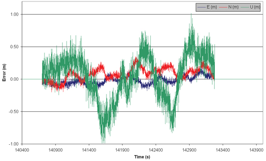
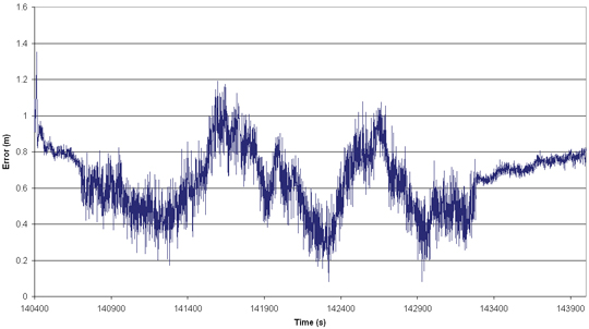
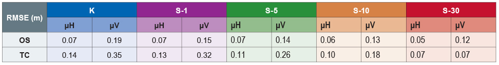
    Comparison to Traditional Estimation. The combined algorithm was tested on multiple sets of off-air data from the U.S., Canada, and the U.K. The root-mean-square error of the horizontal position estimates and the mean geometric dilution of precision during the observations for each of the tested off-air data sets are shown in Table 1. The error magnitudes of the resulting position solutions are on the same order for both the standard pseudorange least-squares and time-free position estimates. This is to be expected, for if the time-free algorithm computes the correct integer milliseconds, the algorithm will converge to nearly the same solution as the traditionally determined pseudoranges since the code-phase measurements are identical. In this comparison, both the pseudorange and combined Doppler/time-free algorithms were started assuming an initial receiver position at the center of the Earth. As a final check that this method provides comparable results to those from the traditional pseudorange case, we directly compared the error magnitudes of the two methods over a stretch of the same data. This will also prove to illustrate how time-free positioning is capable of more quickly estimating the position than other methods since it does not need to decode the satellite signal’s navigation message.

    Nicholas Othieno and Scott Gleason

    TABLE 1. Root-mean-square (R.M.S.) error and geometrical dilution of precision (GDOP) for off-air GPS data sets used with the fastGPS software receiver.

    Table 1. Root-mean-square (R.M.S.) error and geometrical dilution of precision (GDOP) for off-air GPS data sets used with the fastGPS software receiver.

    Figure 7 shows the performance for the combined Doppler/time-free and traditional pseudorange methods together for a period of 34 seconds. As shown, the combined Doppler/time-free positioning algorithm provides receiver position estimates that are comparable in error magnitude to the traditional method. Similar results were obtained for all of the other off-air data sets at our disposal.

    Nicholas Othieno and Scott Gleason
    FIGURE 7 Comparison of position estimation error magnitudes for time-free and traditional pseudorange-based position estimations. Error magnitudes for both methods tested on the Montreal off-air data set.

    Concluding Remarks

    In this article, we have demonstrated that that a GNSS receiver can estimate its position using a snapshot of sampled data and no knowledge of the position of the receiver in low and medium dynamics environments. This addresses an existing limitation of the time-free GNSS navigation technique and facilitates new receiver designs based on limited sampled data sets, notably those using software-based processing techniques. It has been shown that by roughly estimating the receiver position using Doppler measurements with no knowledge of the receiver position, a time-free position estimation can be robustly performed. The limitations on this combined method are due mainly to the dynamic environment of the receiver, which will degrade the rough Doppler position estimate. Nevertheless, this technique will work for a wide range of GNSS applications. Additionally, Monte-Carlo simulations have been performed that show that this combined technique is robust within the stated dynamics limitations and initialization requirements of the time-free method for GPS C/A-code signals.

    Overcoming the Velocity Limitation. The degradation of the Doppler estimation for receivers at higher velocity can be addressed in a number of ways. The most direct correction to this problem is the inclusion of a simple inertial device on the receiver. This will provide a coarse estimate of the receiver velocity that then can be included in the Doppler estimation and would result in position accuracies using Doppler on the order of 1 kilometer in nearly all dynamic receiver cases (limited only by the capability of the inertial sensor).

    The second possibility is to wait for the next generation of GNSS signals to solve the problem for us. Several new GNSS signals (some of which are already being transmitted by active satellites) have been designed with code repeat periods of significantly longer than 1 millisecond (see FIGURE 8). The 1-millisecond code repeat period effectively limits the Doppler estimation error to what was shown above.

    Nicholas Othieno and Scott Gleason
    FIGURE 8. Comparison of code-phase repeat period ambiguities for various GNSS signals.

    Longer repeat periods will correspondingly increase the tolerance of the time-free a priori initialization. Some of the next generation GNSS signals and their respective code repeat periods will be significantly longer than GPS L1 C/A-code. For example, the 20-millisecond code repeat period of the new GPS L2 civil signal corresponds to approximately a 6,000-kilometer repeat length, and an integer 20-millisecond ambiguity of normally only three or four. This will make the construction of the full pseudorange from a 20-millisecond tracking-loop measurement much easier in the presence of larger errors in the a priori position knowledge.

    Discussion. Our work provides a useful method to greatly reduce the processing load in a GNSS receiver, and eliminates the task of decoding GNSS navigation data and the need to have coarse position information. These two advantages together provide a useful step in the development of a dramatically different approach in GNSS signal processing and position estimation. As opposed to existing GNSS receivers, which continually process the incoming signals, this technique allows for strict management of the incoming data and position estimation outputs. This management is well suited for applications that are required to remain off or in a low-power state for long and intermittent periods. Using this technique, any platform can estimate its position by operating the GNSS receiver for a short (snapshot) period of time. The logged data captured during this brief time can then be processed in real time or archived and processed later as the application demands. Applications such as animal tracking or long-duration vehicle tracking, where a position needs to be tracked over a long period using extremely challenging power resources, will benefit notable from this new technique.

    Software demonstrating the algorithms discussed above can be downloaded free of charge from http://gnssapplications.org/, including Chapter 3 (on the GNSS simulator) and Chapter 5 (on the fastGPS receiver).

    Acknowledgments

    This article is based on the paper “Combined Doppler and Time Free Positioning Technique for Low Dynamics Receivers” presented at PLANS 2012, the Institute of Electrical and Electronics Engineers / Institute of Navigation Position, Location and Navigation Symposium held in Myrtle Beach, South Carolina, April 23–26, 2012.

    Manufacturer

    Tests were conducted using a SparkFun (www.sparkfun.com ) SiGe GN3S USB front end.


    NICHOLAS OTHIENO was an M.A.Sc. student in the Department of Electrical and Computer Engineering at Concordia University, Montreal, Canada. His research was in the area of software-based GNSS techniques and applications.

    SCOTT GLEASON has been an assistant professor in the Department of Electrical and Computer Engineering at Concordia University since 2010. He received his B.S. degree in electrical and computer engineering from the State University of New York at Buffalo, an M.S. in engineering from Stanford University, and a Ph.D. from the University of Surrey in England. He has worked in the areas of astronautics, remote sensing, and GNSS for more than 15 years, including time at NASA’s Goddard Space Flight Center and Stanford’s GPS Laboratory, and the National Oceanography Centre, Southampton, England.


    FURTHER READING

    • Authors’ Publications

    “Combined Doppler and Time Free Positioning Technique for Low Dynamics Receivers” by N. Othieno and S. Gleason in Proceedings of PLANS 2012, the Institute of Electrical and Electronics Engineers / Institute of Navigation Position, Location and Navigation Symposium held in Myrtle Beach, South Carolina, April 23–26, 2012, pp. 60–65.

    Combined Doppler and Time-Free Navigation for Low Dynamics Receivers by N. Othieno, M.A.Sc. thesis, Department of Electrical and Computer Engineering, Concordia University, Montreal, Canada, April 2012.

    • Assisted GNSS

    A-GPS: Assisted GPS, GNSS, and SBAS by F. van Diggelen, published by Artech House, Boston, Massachusetts, 2009.

    Assisted GPS: A Low-Infrastructure Approach” by J. LaMance, J. DeSalas, and J. Järvinen in GPS World, Vol. 13, No. 3, March 2002, pp. 46–51.

    • New GNSS Signals

    “New Navigation Signals and Future Systems in Evolution” by A.R. Pratt, Chapter 17 in GNSS Applications and Methods, eds. S. Gleason and D. Gebre-Egziabher, Artech House, Boston, Massachusetts, 2009.

    • Software GNSS Receivers and Simulators

    Software GNSS Receiver: An Answer for Precise Positioning Research” by T. Pany, N. Falk, B. Riedl, T. Hartmann, G. Stangl, and C. Stöber in GPS World, Vol. 23, No. 9, September 2012, pp. 60–66.

    Digital Satellite Navigation and Geophysics: A Practical Guide with GNSS Signal Simulator and Receiver Laboratory by I.G. Petrovski and T. Tsujii with foreward by R.B. Langley, published by Cambridge University Press, Cambridge, U.K., 2012.

    “GNSS Navigation: Estimating Position, Velocity, and Time” by S. Gleason and D. Gebre-Egziabher, Chapter 3 in GNSS Applications and Methods, eds. S. Gleason and D. Gebre-Egziabher, Artech House, Boston, Massachusetts, 2009.

    “A GPS Software Receiver” by S. Gleason, M. Quigley, and P. Abbeel, Chapter 5 in GNSS Applications and Methods, eds. S. Gleason and D. Gebre-Egziabher, Artech House, Boston, Massachusetts, 2009.

    “A Real-Time Software Receiver for the GPS and Galileo L1 Signals” by B.M. Ledvina, M.L. Psiaki, T.E. Humphreys, S.P. Powell, and P.M. Kintner Jr. in Proceedings of ION GNSS 2006, the 19th International Technical Meeting of the Satellite Division of The Institute of Navigation, Fort Worth, Texas, September 26–29, 2006, pp. 2321–2333.

    “Architecture of a Reconfigurable Software Receiver” by G.W. Heckler and J.L. Garrison in Proceedings of ION GNSS 2004, the 17th International Technical Meeting of the Satellite Division of The Institute of Navigation, Long Beach, California, September 21–24, 2004, pp. 947–955.

    • Use of Doppler Measurements in GNSS Positioning and Navigation

    Doppler-Aided Positioning: Improving Single-Frequency RTK in the Urban Environment” by M. Bahrami and M. Ziebart in GPS World, Vol. 22, No. 5, May 2011, pp. 47–56.

    “Instantaneous Real-Time Cycle-Slip Correction for Quality Control of GPS Carrier-Phase Measurements” by D. Kim and R.B. Langley in Navigation, Vol. 49, No. 4, Winter, 2002–2003, pp. 205-222.

    “The Principle of a Snapshot Navigation Solution Based on Doppler Shift” by J. Hill in Proceedings of ION GPS 2001, the 14th International Technical Meeting of the Satellite Division of The Institute of Navigation, Salt Lake City, Utah, September 11–14, 2001, pp. 3044–3051.

    Measuring Velocity Using GPS” by M.B. May in GPS World, Vol. 3, No. 8, September 1992, pp. 58–65.

    “Geometrical Aspects of Differential GPS Positioning” by P. Vaníček, R.B. Langley, D.E. Wells, and D. Delikaraoglou in Bulletin Géodésique, Vol. 58, No. 1, 1984, pp. 37–52, doi: 10.1007/BF02521755.

  • Galileo’s Surveying Potential: E5 Pseudorange Precision

    By Ismael Colomina, Christian Miranda, M. Eulàlia Parés, Marcus Andreotti, Chris Hill, Pedro F. da Silva, João S. Silva, Tiago Peres, João F. Galera Monico, Paulo O. Camargo, Antonio Fernández, José Maria Palomo, João Moreira, Gustavo Streiff, Emerson Z. Granemann, and Carmen Aguilera

    New Galileo signals have great potential for pseudorange-based surveying and mapping in both optimal open-sky conditions and suboptimal under-canopy environments. This article reviews the main features of Galileo’s E5 AltBOC and E1 CBOC signals, describes generation of realistic E5 and E1 pseudoranges with and without multipath sources, and presents anticipated horizontal positioning accuracy results, ranging from 4 centimeters (open-sky) to 14 centimeters (under-canopy) for E5/E1.

    The history of GNSS surveying has been written in the carrier phase language — until now. The well known reason for this is the high precision, at the millimeter level, of the carrier phase observables and the low precision, at half a meter or worse, of the pseudorange observables. The progress and results of carrier-phase positioning are also well known and, today, surveyors can count on many effective ways for relative and absolute, static and kinematic, accurate positioning procedures like RTK, PPP and others. On the other hand, pseudorange observables have been used for various cadastral, GIS and mapping applications with meter and lower level accuracy requirements. The main advantages of pseudorange positioning are the simplicity and robustness of data processing. Moreover, the typical user of GNSS (pseudorange) mapping gear needs less GNSS education and training than the typical GNSS geodetic surveyor.

    However, there are cadastral and mapping applications that require better accuracies than current pseudoranges provide and there are surveying applications that do not require the cm to dm level accuracies that carrier phases provide. There is a gap where no choice is optimal: either the choice is unnecessarily expensive (receivers, processing software, trained personnel) or it is unacceptably inaccurate. This gap can be reduced or eliminated with the new GPS and Galileo signals. It is therefore convenient that the size of the new smaller gap, if any, be analyzed as soon as possible even if the analysis has to rely on simulated signals.

    According to the simulations performed, it is expected that pseudoranges can be extracted from the Galileo E5 AltBOC signals with tracking errors (1-σ level) ranging from 0.02 m (“open sky” scenarios) to 0.08 m (“tree covered” scenarios with 15% through-foliage visibility) whereas for the Galileo E1 CBOC signals the tracking errors range between 0.25 m and 2.00 m respectively. With these tracking errors and with the explicit estimation of the ionosphere parameters, the available simulations indicate “open sky” horizontal/vertical accuracies of 0.04/0.17 m for static positioning and 0.04/0.20 m ones for (low dynamics) kinematic positioning; and “tree covered” accuracies of 0.05-0.13/0.07-0.30 m for static positioning and 0.15/0.35 m for (low dynamics) kinematic positioning.

    The high precision of the Galileo E5 AltBOC range measurements suggests that their modeling can benefit from available research results of the precise point positioning (PPP) carrier phase-based techniques. Since, in contrast to carrier phase measurements, pseudoranges are not ambiguous, it is expected that the convergence challenges of PPP will disappear or largely be mitigated when using cm-level precise pseudoranges. As a result, in addition to standard relative positioning surveying, absolute positioning surveying is likely to emerge as a standard procedure, both in real-time (using Galileo ultra-rapid orbits hopefully available in future from the IGS) or in post-processing (similarly, using IGS final precise Galileo orbits). Clearly, the question is how fast and how well the unknown parameters in the pseudorange model will converge to the correct values. However, even low convergence might be a minor problem as, with pseudoranges, loss-of-lock situations do not require the re-initialization of some parameters in the estimation algorithms.

    Absolute pseudorange positioning is of particular interest because simple GNSS surveying with pseudoranges can become a practical tool in regions with sparse GNSS permanent station distributions and for communities with limited surveying expertise. As the results and behavior of E5 AltBOC pseudorange positioning consolidate and become well understood, appropriate surveying procedures will be identified and adopted. The starting point for this is the investigation of static (absolute) and kinematic (with known initial/end points) positioning with E5 AltBOC and E1 CBOC.

    The full deployment of the Galileo constellation — Full Operational capability (FOC) — is currently scheduled for 2020. As of now, two satellites of the In-Orbit Validation (IOV) have been launched and two more will follow that will complement the two experimental satellites (GIOVE-A and GIOVE-B) already in orbit. The Initial Operational Capability (IOC) is scheduled for 2014 and will include fourteen satellites that were ordered in January 2010. In addition to this, eight additional satellites have been ordered in February 2012.

    Although not covered in this paper, we note that there are a number of potential ways to benefit from the E5 AltBOC signal and modulation before Galileo FOC. One of them is to combine the E1/E5 Galileo signals with the L1/L5 GPS signals and “replace” the missing Galileo signals with GPS ones. Another one that will depend on the IOV satellite configuration is to keep on working with full GPS L1/L2 satellite constellations and “assist” GPS with Galileo to speed up convergence periods in PPP or to extend the ranges of Differential GPS (DGPS).

    In the paper we concentrate on the combination of E1 CBOC and E5 AltBOC signals and modulations by explicitly estimating the ionospheric bias — or a correction with respect to a model — instead of forming ionospheric-free combinations. The reason for this is that, since the E1 CBOC and E5 AltBOC pseudoranges have disparate noise levels, in the resulting ionospheric-free pseudoranges the low noise properties of E5 AltBOC will be lost. (We note the alternative method, in the presence of precise pseudoranges, of taking advantage of the ionospheric divergence of carrier phase and pseudoranges. In this approach I sr or δI sr are estimated with the use of just the E5 frequency.)

    The research reported in this paper has been conducted in the frame of the international –EU and Brazil – ENCORE project. ENCORE –Enhanced Code Galileo Receiver for Land Management in Brazil – is funded by the European Commission (grant 247939) with the aim to implement the 7th European Framework Program for Research and Development (FP7). The project runs from 2010 to 2012 and is realized by a European-Brazilian consortium lead by DEIMOS Engenharia (Portugal). The goals of ENCORE are the introduction of Galileo terminals in the Brazilian market for land management applications, the stimulation of the participation of Brazilian entities in Galileo and the development of a high-precision and low-cost land management application based on Galileo signals.

    The Galileo Signals

    The development of new GNSS systems, as the Galileo system (as well as the modernization of currently available ones, as the GPS) will provide additional signals with increasingly complex modulations and multiplexing schemes, enabling performance enhancements in terms of availability, accuracy, and robustness.

    Tracking accuracy and multipath robustness are closely related to the slope of the (main) peak of the Auto-Correlation Function (ACF) of the signals. Figure 1 shows the ACFs for the most relevant GPS and Galileo modulations. Figure 2 shows the multipath error envelopes for the corresponding GPS and Galileo signals when using an Early-Late Power discriminator and a correlator spacing of 0.1 chip (assuming one reflected ray and a carrier over multipath ratio of 2).

     Figure 1. Normalized auto-correlation functions for different modulations: BPSK (n) of GPS L1, BOC (n,n) of Galileo E1 with simplified demodulation, CBOC (6n,n,1/11) of Galileo E1, and AltBOC (1.5n,n) of Galileo E5 signals. By Ismael Colomina, Christian Miranda, M. Eulàlia Parés, Marcus Andreotti, Chris Hill, Pedro F. da Silva, João S. Silva, Tiago Peres, João F. Galera Monico, Paulo O. Camargo, Antonio Fernández, José Maria Palomo, João Moreira, Gustavo Streiff, Emerson Z. Granemann, and Carmen Aguilera
    Figure 1. Normalized auto-correlation functions for different modulations: BPSK (n) of GPS L1, BOC (n,n) of Galileo E1 with simplified demodulation, CBOC (6n,n,1/11) of Galileo E1, and AltBOC (1.5n,n) of Galileo E5 signals.

    Multiplexed BOC (MBOC) is a new modulation introduced in 2006, and included recently in the Galileo SIS ICD. The E1 Open Service modulation receives the name of Composite Binary Offset Carrier (CBOC) and is a particular implementation of MBOC. The CBOC (6,1,1/11) modulation is the result of a linear combination of a wideband BOC (6,1) sub-carrier with a narrow-band BOC (1,1) sub-carrier, in such a way that 1/11 of the power is allocated (in average) to the high frequency component.

    The Galileo CBOC (6,1,1/11) signal’s demodulation can be simplified by using a BOC (1,1) modulated local replica, at the expense of tracking and multipath robustness performance (making it comparable to that of a BOC (1,1) signal) but enabling an interesting trade-off between performance and receiver complexity. In the current work the CBOC modulation is assumed.

    Nevertheless, the potential of the future Galileo E5 signal is expected to outshine even these modernized signals. The Galileo E5 signal, with its Alternative Binary Offset Carrier (AltBOC) modulation, is one of the most advanced and promising signals of the Galileo system. Receivers capable of tracking this signal will benefit from unequalled performance in terms of measurement accuracy, precision, and multipath suppression. However, the signal processing techniques to implement a matched-filter AltBOC demodulation are much more challenging than those for the traditional BPSK or even for the BOC modulations (as the current GPS L1 C/A or future L1 C signals). This stems from the large bandwidth (chip rate), complex sub-carrier, elaborate multiplexing scheme (which enables the simultaneous broadcast of 4 channels on a single carrier) and complex interaction of the 4 multiplexed channels.

    The AltBOC (15,10) correlation peak is similar to the one of BOC(15,10) near the main peak and, as suggested in Figures 1 and 2, it outperforms all other modulations of the current and future GPS and Galileo civil and open service signals (note that the x axis of Figure 1 is also normalized by the chip period, which is 10 times shorter for the AltBOC (15,10) modulation than for the remaining ones).

     Figure 2. Multipath error envelopes for GPS L1 (BPSK(1)), Galileo E1 (demodulated as BOC (1,1) and CBOC (6,1,1/11)), and Galileo E5 AltBOC (15,10) signals (Early-Late Power discriminator, correlator spacing of 0.1 chip, carrier over multipath ratio of 2 and infinite bandwidth). By Ismael Colomina, Christian Miranda, M. Eulàlia Parés, Marcus Andreotti, Chris Hill, Pedro F. da Silva, João S. Silva, Tiago Peres, João F. Galera Monico, Paulo O. Camargo, Antonio Fernández, José Maria Palomo, João Moreira, Gustavo Streiff, Emerson Z. Granemann, and Carmen Aguilera
    Figure 2. Multipath error envelopes for GPS L1 (BPSK(1)), Galileo E1 (demodulated as BOC (1,1) and CBOC (6,1,1/11)), and Galileo E5 AltBOC (15,10) signals (Early-Late Power discriminator, correlator spacing of 0.1 chip, carrier over multipath ratio of 2 and infinite bandwidth).

    The E5 signal can be separated into two sub-bands (E5a and E5b) which can be treated separately by a Galileo E5 receiver (as BPSK (10) modulated signals), called Single Side-Band (SSB) processing. However, this would result in the loss of the promising AltBOC signal properties (resulting in a classical triangular ACF). Hence, a matched filter demodulation of the full Galileo E5 signal is desired to implement the best possible receiver in terms of accuracy and multipath robustness, at the expense of an increase in the receiver complexity and required bandwidth.

    The existence of secondary peaks (as shown in Figure 1) in the ACFs of Binary Offset Carrier (BOC) modulations (as the AltBOC and CBOC) require specific techniques (i.e., bump-jumping) to ensure that the main peak is the one being tracked.

    According to the simulations performed, in the absence of multipath or signal fading sources the performances achievable with E5 AltBOC and E1 CBOC in terms of accuracy of the code tracking errors is 0.02 m and 0.25 m respectively at 45 degree (about 40 dB-Hz for E1 and 44 dB-Hz for E5) with a correlator spacing of 0.1 chip and integration times of 4 ms.

    If multipath and signal fading sources are present, the expected errors increase to 0.08 m and 2 m respectively (for about 36 dB-Hz for E1 and 40 dB-Hz for E5). Longer integration times will lead to better performances.

    During the project, the above simulation results will be compared against those obtained with Galileo live signals. Figure 3 shows the ENCORE hardware receiver prototype, which is composed by the FPGA board, the RF FE board, the LNA and the antenna. The mezzanine board and the two voltage converters, which can also be seen in figure, enable the receiver testing using recorded IF signals or synthetic IF data.

     Figure 3. ENCORE hardware receiver prototype. By Ismael Colomina, Christian Miranda, M. Eulàlia Parés, Marcus Andreotti, Chris Hill, Pedro F. da Silva, João S. Silva, Tiago Peres, João F. Galera Monico, Paulo O. Camargo, Antonio Fernández, José Maria Palomo, João Moreira, Gustavo Streiff, Emerson Z. Granemann, and Carmen Aguilera
    Figure 3. ENCORE hardware receiver prototype.

    Positioning Models and Algorithms

    The observation equations for pseudorange measurements follow the modelling principles of PPP. Thus, the observed pseudoranges P1sr (E1 CBOC) and P5sr (E5 AltBOC) can be modeled as

    Screen shot 2013-01-04 at 7.17.32 PM .By Ismael Colomina, Christian Miranda, M. Eulàlia Parés, Marcus Andreotti, Chris Hill, Pedro F. da Silva, João S. Silva, Tiago Peres, João F. Galera Monico, Paulo O. Camargo, Antonio Fernández, José Maria Palomo, João Moreira, Gustavo Streiff, Emerson Z. Granemann, and Carmen Aguilera (1)

    for i = 1,5, where ρsr is the true geometric distance between satellite s and receiver r, c is the speed of light in a vacuum, δts is the given s satellite clock correction, R s is the relativistic “correction” for satellite s, T sr is the modelled or given tropospheric delay, f1, f5 are the frequencies of E1 CBOC and E5 AltBOC respectively, I sr / f 2i are the modelled or given ionospheric delays, and bis are the given biases for satellite s.

    In the above pseudorange observation equation, we will estimate the receiver position Xr (included in ρ sr ), the receiver clock correction δtr , the correction δT sr to the modelled or given tropospheric delay T sr , the term δI sr related to the correction δI sr / f 2i to the modelled or given ionospheric delays I sr / f 2i , and the receiver frequency dependent biases bir. In equation 1, ρsr is a well-known function of the satellite ephemeris, the receiver position, the satellite and receiver antenna phase centre offsets, and of all the effects, like solid Earth tides, usually included in PPP models.

    The time dependent unknown parameters in equation 1 are further modelled as random walk stochastic processes for the stochastic differential equation of the prediction step (Kalman filter estimation approach) or of the dynamic model (dynamic network estimation approach) as follows: δtr is a random walk with rather large driving white noise variance [rw (∞)]; δT sr as rw (0.0152 m2), PSD level; bir as rw (0.00172 m2), PSD level (b1r is set to 0); and (I sr + δI sr ) / f 2i as rw (σ2 m 2 ) with

    Screen shot 2013-01-04 at 7.17.45 PM . By Ismael Colomina, Christian Miranda, M. Eulàlia Parés, Marcus Andreotti, Chris Hill, Pedro F. da Silva, João S. Silva, Tiago Peres, João F. Galera Monico, Paulo O. Camargo, Antonio Fernández, José Maria Palomo, João Moreira, Gustavo Streiff, Emerson Z. Granemann, and Carmen Aguilera(2)

    where Screen shot 2013-01-04 at 7.25.01 PM, T = 64 × 60 s, and τ is the time interval (in seconds) between two successive measurements. Clearly, the stochastic model for the total ionospheric delay depends on assumptions for Screen shot 2013-01-04 at 7.25.59 PMand T that also depend on the solar activity. Furthermore, depending on the model or data used for I sr the actual parameter to be estimated δI sr and, specifically δI sr , / f 2i will obey to different “amplitude” and “time correlation” T values. For the results reported in the paper, the three-dimensional, time dependent ionospheric electron density NeQuick model was used for I sr . For δI sr , / f 2i , the values Screen shot 2013-01-04 at 7.26.54 PM . By Ismael Colomina, Christian Miranda, M. Eulàlia Parés, Marcus Andreotti, Chris Hill, Pedro F. da Silva, João S. Silva, Tiago Peres, João F. Galera Monico, Paulo O. Camargo, Antonio Fernández, José Maria Palomo, João Moreira, Gustavo Streiff, Emerson Z. Granemann, and Carmen Aguilera, T = 5 × 60 s, were adopted.

    In the ENCORE project, the above models are being used to investigate the performance of the various positioning modes (absolute and relative, static and kinematic) and procedures (with and without a “ground presurveyed” or “ground control” point in the absolute positioning mode).

    Simulation Scenarios

    Due to the unavailability of sufficient Galileo space vehicles at the moment, the validation of the algorithms described before was done using the Navigation Sensor Simulation (NSS) tool, developed by University of Nottingham. The NSS data simulation tool was originally designed to simulate the types of measurements that can be made using a GNSS receiver. Specifically the simulator has the capability of producing code, carrier and Doppler measurements on L1, E1, E5a, E5b, E5 (combined), L2c, L5, and E6 frequencies, covering GPS and Galileo systems. The simulation is achieved by using the true locations of both the receiver and the satellites to calculate the true, error-free measurements. Error models are then applied to account for the various inaccuracies seen in real-world measurements. The simulation results are returned to the user in a file in the standard Receiver Independent Exchange (RINEX) observations format.

    The user of the NSS tool is required to define a simulation scenario. The main inputs from a scenario definition are the satellite ephemeris data and the true location of the receiver as well as the parameters for the various error models and the time period for which data should be simulated. It is possible to simulate data using the true locations of the satellites for any day in the past.

    For the purpose of this work, the precise orbits used for the Galileo system were obtained from the GalileoSat System Simulation Facility (GSSF) simulator. The expected error on the estimated values for BGD (E1 E5a) and BGD (E1 E5b) was also applied,

    NSS provides models for the two types of discriminator widely used in GPS receivers: the Early-Minus-Late Power (EMLP) and the Dot-Product (DP) discriminators. For this, NSS accepts parameters for front-end filter bandwidth, correlator spacing, DLL loop bandwidth and integration time for each of the signal modulations it is capable to work with: GPS BPSK (1), GPS BPSK (10), Galileo CBOC (6, 1, 1/11), and Galileo AltBOC (15, 10).

    Table1 . By Ismael Colomina, Christian Miranda, M. Eulàlia Parés, Marcus Andreotti, Chris Hill, Pedro F. da Silva, João S. Silva, Tiago Peres, João F. Galera Monico, Paulo O. Camargo, Antonio Fernández, José Maria Palomo, João Moreira, Gustavo Streiff, Emerson Z. Granemann, and Carmen Aguilera
    Table 1. Galileo orbit error factors applied.
     Table 2. Parameters for the generation of the simulated pseudoranges. By Ismael Colomina, Christian Miranda, M. Eulàlia Parés, Marcus Andreotti, Chris Hill, Pedro F. da Silva, João S. Silva, Tiago Peres, João F. Galera Monico, Paulo O. Camargo, Antonio Fernández, José Maria Palomo, João Moreira, Gustavo Streiff, Emerson Z. Granemann, and Carmen Aguilera
    Table 2. Parameters for the generation of the simulated pseudoranges.

    C/No values for GPS and Galileo for various satellite elevation angles are tabled inside NSS in accordance with measurements available from various sources. The values in those tables are interpolated via respective spline equations for intermediate elevation angles.

    For the scope of the ENCORE project and its application for land management in rural areas, it is assumed that the influence of the vegetation on the satellite signals will be of creating diffuse, non-coherent signal scattering, resulting in signal loss but not significantly in signal delay. Therefore the ITU-R model is of greater interest as this model gives empirical values of cumulative signal fade due to tree shadowing, based in multiple measurement campaigns. The ITU-R signal fading model takes as input the signal frequency, the satellite elevation angle and the “estimated signal visibility percentage” of the signal. This last parameter accounts for the foliage effect on the signal, and will have a low value when the tree is in full foliage and a high value when the trees are without leaves.

    For the tropospheric delay, NSS makes use of the EGNOS Troposphere Model, although in NSS this model is used to simulate the delay experienced due to the troposphere rather than correct for it. For the ionospheric delay, NSS has been developed to read Total Electron Content (TEC) maps in the standard IONEX file format. These files may contain 2 or 3 dimensional maps of the TEC at a number of equally spaced epochs, usually covering a 24 hour period. The TEC for each sub-ionospheric pierce point at a given epoch is calculated by interpolating between two TEC maps at consecutive epochs. The maps are firstly rotated around the z-axis to compensate for the strong correlation between the ionosphere and the sun’s position. A standard 4 point interpolation scheme is then used to interpolate each TEC map to the required latitude and longitude.

    The scenario definition is completed by selecting the number and type of measurements to be simulated along with the data interval for the measurements and the elevation masking angle of the receiver.

    The preliminary results presented in this paper are based on simulation scenarios created from the base settings presented in tables 1 and 2, for the “open sky” (OS) and “tree covered” (TC) cases, using 8 Galileo satellites (of a 27-satellite constellation) for a fixed point in Brazil that has been processed in the absolute and static/kinematic modes. Thus 10 cases have been investigated that result from combining the OS and TC ones with the kinematic (K) and static (S) cases. The static cases have been computed for observation periods of 1, 5, 10 and 30 minutes respectively (cases S-1, S-5, S-10 and S-30). For all test cases a 45 minute data set measured at 1 Hz has been processed together with start/end initialization periods –i.e., observations processed in the static mode– of 5/10 minutes respectively. Thus, the test OS S-5 (confer table 3) corresponds to the “open sky” scenario for static point determination with observation periods of 5 minutes and the test TC-K corresponds to the “tree covered” scenario for kinematic point determination at 1 Hz.

    Results from Simulated Measurements

    Table 3 summarizes the results of the tests described in the previous section. Each table cell contains the Root Mean Square Error (RMSE) of the horizontal (μH) and vertical (μV) positioning results when compared to the known true value of the fixed point established for the simulations. Figures 4 to 7 represent the receiver’s position and clock errors for the OS and TC cases. Note again, that positioning is performed in the absolute and post-processing mode.

    Col-4 . By Ismael Colomina, Christian Miranda, M. Eulàlia Parés, Marcus Andreotti, Chris Hill, Pedro F. da Silva, João S. Silva, Tiago Peres, João F. Galera Monico, Paulo O. Camargo, Antonio Fernández, José Maria Palomo, João Moreira, Gustavo Streiff, Emerson Z. Granemann, and Carmen Aguilera
    Figure 4. Position accuracy for the Open Sky scenario, case K.
     Figure 5. Receiver’s clock accuracy for the Open Sky scenario, case K. By Ismael Colomina, Christian Miranda, M. Eulàlia Parés, Marcus Andreotti, Chris Hill, Pedro F. da Silva, João S. Silva, Tiago Peres, João F. Galera Monico, Paulo O. Camargo, Antonio Fernández, José Maria Palomo, João Moreira, Gustavo Streiff, Emerson Z. Granemann, and Carmen Aguilera
    Figure 5. Receiver’s clock accuracy for the Open Sky scenario, case K.
     Figure 6. Position accuracy for the Tree Covered scenario, case K. By Ismael Colomina, Christian Miranda, M. Eulàlia Parés, Marcus Andreotti, Chris Hill, Pedro F. da Silva, João S. Silva, Tiago Peres, João F. Galera Monico, Paulo O. Camargo, Antonio Fernández, José Maria Palomo, João Moreira, Gustavo Streiff, Emerson Z. Granemann, and Carmen Aguilera
    Figure 6. Position accuracy for the Tree Covered scenario, case K.
     Figure 7. Receiver’s clock accuracy for the Tree Covered scenario, case K. By Ismael Colomina, Christian Miranda, M. Eulàlia Parés, Marcus Andreotti, Chris Hill, Pedro F. da Silva, João S. Silva, Tiago Peres, João F. Galera Monico, Paulo O. Camargo, Antonio Fernández, José Maria Palomo, João Moreira, Gustavo Streiff, Emerson Z. Granemann, and Carmen Aguilera
    Figure 7. Receiver’s clock accuracy for the Tree Covered scenario, case K.

    Although the results can still be considered preliminary, they illustrate what can be expected from the proposed combination of E1 and E5 Galileo pseudoranges. The horizontal accuracy estimator μH is computed as μH=√ μ2E + μ2N where μE , μN are the position RMSE in the North and East components respectively; μV is the position RMSE in the height component. In the OS scenario, the horizontal accuracy estimator is always below 10 centimeters and is rather independent of the processing mode as the horizontal accuracy of kinematic positioning (μH = 7 centimeters) does not differ much from that of half-an-hour positioning (μH = 5 centimeters). When, in the future, actual Galileo E1 and E5 measurements can be used instead of simulated ones, it is likely that remaining unmodelled systematic errors slightly worsen the reported positioning accuracy. As usual, this can be overcome with differential positioning at the expense of loosing some precision. On the other side, an easy and robust procedure for absolute positioning is of interest for land surveying and cadastral mapping of vast areas. The mentioned values, even if they may seem optimistic because of their simulated origin, still fall comfortably within the specifications of the official Brazilian National Institute for Colonization and Agrarian Reform (INCRA) for all surveying categories down to the fundamental C1 ( μH = 10 cm). In Figure 4, the results of the kinematic positioning simulation exhibit a remaining systematic, rather constant and at the few cm level, error dominating the N and E horizontal components. The vertical error is much noisier than the horizontal one and this behaviour may indicate that further research on the overall modelling of the combined E5/E1 signals is required. However, model fine tuning in the absence of actual signals has its limitations and dangers and, therefore, no big effort has been devoted to this issue. Last but not least, vertical accuracy ranges between μV = 19 centimeters for kinematic positioning and μV = 12 centimeters, for the kinematic and half-an-hour static cases respectively. The same discussion applies here as for the horizontal case, when the actual Galileo signals become available.

    Table 3 also contains the corresponding RMSE results for the TC case. As expected they are worse than those of the OS case and range between μH = 14 cm (kinematic case) to μH = 7 cm (half-an-hour static case). In all cases, they would meet the C2 INCRA category (μH = 20 cm). Vertical accuracy ranges from μV = 35 cm (kinematic case) to μV = 18 cm (static case, S-10) to μV = 0.07 (static case, S-30) although the last S-30 result is thought to be a lucky coincidence rather than a representative figure.

    Table3 . By Ismael Colomina, Christian Miranda, M. Eulàlia Parés, Marcus Andreotti, Chris Hill, Pedro F. da Silva, João S. Silva, Tiago Peres, João F. Galera Monico, Paulo O. Camargo, Antonio Fernández, José Maria Palomo, João Moreira, Gustavo Streiff, Emerson Z. Granemann, and Carmen Aguilera
    Table 3. Empirical results (errors) of point positioning for the E1/E5 combination (click to enlarge).

    Conclusions and Ongoing Work

    We have discussed the potential of the combination of Galileo E1 CBOC and E5 AltBOC pseudoranges for surveying and mapping applications in the frame of the international cooperation Galileo project ENCORE. Via simulations, we have investigated the tracking precision of the E1 and E5 pseudoranges under “open sky” and strong “tree coverage” scenarios resulting in 0.25 to 2.00 m (E1) and 0.02 to 0.08 m (E5) pseudorange precisions. We have further investigated the post-processed results — therefore with final precise Galileo orbits — in the OS and TC scenarios cases for kinematic and static modes and given preliminary results.

    According to them, in the OS case, the positioning accuracy of the used E1/E5 combination and parameter estimation approach is at the cm-level for the E, N horizontal components and at the dm level for the height component. In the TC case, the accuracy estimates are at the low dm-level for the horizontal components and at the dm-level for the vertical ones. In the OS case, the INCRA C1 tolerances are met and in the TC case, the C2 tolerances are met. The accuracy estimates are at the low dm-level for the horizontal components and at the dm-level for the vertical one.

    In the next months, up to the completion of the ENCORE project, we plan on extending the simulation analysis to the whole scenario spectra, with and without a complete Galileo constellation, with and without GPS L1/L5 measurements, in static and kinematic modes, in real-time and post-processing modes, and with precision and broadcast orbits. In parallel, we also plan to finish the E5/E1 ENCORE prototype receiver and software, a joint effort of DEIMOS Engenharia and OrbiSat da Amazônia, a Brazilian consortium member.

    Acknowledgments

    The reported research has been conducted within the “Enhanced Code Galileo Receiver for Land Management in Brazil” (ENCORE) project funded by the European Commission (grant 247939) with the aim to implement the 7th European Framework Program for Research and Development (FP7). The project runs from 2010 to 2012 and is realized by a European-Brazilian consortium lead by DEIMOS Engenharia (Portugal) and with participation of DEIMOS Space (Spain), the Institute of Geomatics (Spain), the Institute of Engineering Surveying and Space Geodesy of the University of Nottingham (UK), the São Paulo State University (UNESP, Brazil), OrbiSat da Amazônia (Brazil), Santiago e Cintra (Brazil) and MundoGeo (Brazil).


    Ismael Colomina is director of the Institute of Geomatics (IG) of Spain, holds a Ph.D. in mathematics from the University of Barcelona (UB), and is a member of GPS World’s Editorial Advisory Board.

    Christian Miranda received his MSc in telecommunication engineering and management from Universitat Politècnica de Catalunya. He is a research assistant at the IG.

    M. Eulàlia Parés holds an MSc in meteorology and vlimatology (UB) and an MSc in airborne photogrammetry and remote sensing (IG). She is a research assistant and PhD candidate at the IG.

    Marcus Andreotti received a Ph.D. in engineering surveying from the University of Nottingham (UN), where he was a research associate at the Institute of Engineering Surveying and Space Geodesy (IESSG). He is currently with NovAtel, Canada.

    Chris Hill is a principal research fficer at the IESSG, holding a Ph.D. in satellite laser ranging.

    Pedro F. Silva received his aerospace engineering degree from Instituto Superior Técnico (IST), Portugal. He works at DEIMOS Engenharia as head of the GNSS Division.

    João S. Silva received his aerospace engineering degree from IST. He is currently a project manager in DEIMOS Engenharia’s GNSS Technologies Division.

    Tiago Peres received his MSc degree in Aerospace Engineering from Instituto Superior Técnico, Portugal. He is a Project Engineer in the GNSS Technologies Division of DEIMOS Engenharia

    João F. Galera Monico is an associate professor at the Universidade Estadual Paulista (UNESP), Brazil. He is a researcher and consultant of the Brazilian Research Council (CNPq), FAPESP and CAPES.

    Paulo O. Camargo is an assistant doctor at UNESP, developing his post-doctoral activities at the National University of La Plata, Argentina.

    Antonio Fernandez received an MSc degree in aeronautical engineering from the Polytechnical University of Madrid (UPM) and an MSc in physics from the UNED University of Spain. He is head of GNSS Division in the Aerospace Engineering Business Unit at DEIMOS Space, Spain.

    José M. Palomo received a telecommunication engineering degree from the UPM. He works in GNSS receiver technologies and OFDM (WiMax) communication systems at DEIMOS Space.

    João Moreira is technical director of Orbisat da Amazônia Indústria e Aerolevantamento SA. He received his Ph.D. in microwave technology at at theTechnical University of Munich.

    Emerson Z. Granemann graduated in cartographic engineering from the Universidade Federal do Paraná, Brazil. He is founder and chief executive of MundoGEO Publishing.

    Carmen Aguilera is market development officer at the European GNSS Agency. She holds an MSc in telecommunications engineering.


  • Expert Advice: Cause Identified for Pseudorange Error from New GPS Satellite SVN-49

    By Richard Langleuy, with an additional note by Oliver Montenbruck

    The GPS Wing and its contractors have traced the cause of pseudorange errors on L1 and L2 broadcast by the newest GPS satellite, SVN-49, to the manner in which the L5 signal demonstration payload was added to the satellite. Signal leakage between the two input ports of the antenna coupler network for the satellite’s array of 12 helical antenna elements, reflected from the L5 filter and then transmitted, creates a second signal with a delay of approximately 30 nanoseconds, and the appearance of a multipath component.

    While testing an adjustment to the signal-in-space to minimize the effect of the problem on receiver navigation solutions on Earth, the GPS Wing is interested in hearing from manufacturers and the user community concerning the different impacts of SVN-49 signals on the wide range products and applications in operation, before reaching a final decision on what to do with the satellite prior to setting it healthy.


    The seventh modernized GPS Block IIR satellite was launched on March 24, 2009. Called SVN-49, its sequence number in the long line of GPS satellites, or PRN01, after its pseudorandom noise code identifier, this satellite is special. In addition to the equipment required to transmit the legacy GPS C/A-code and P(Y)-code signals and the new civil L2C-code and military M-code signals on the standard L1 (1575.42 MHz) and L2 (1227.6 MHz) frequencies, SVN-49 carries an L5 demonstration payload. L5 is the new civil signal to be transmitted on 1176.45 MHz by Block IIF and succeeding generations of GPS satellites.

    The demo payload was included to claim the frequency, which was allocated by the International Telecommunication Union before the August 26, 2009, deadline. The deadline had been imposed seven years earlier when the GPS Joint Program Office (the forerunner of the GPS Wing) applied for the frequency. The Block IIF program schedule had slipped a bit and as a safeguard (and one which eventually saved the day), the demo payload was developed and assigned to SVN-49.

    Shortly after the L1/L2 system on SVN-49 was activated on March 28, it became clear that the satellite had a small problem. The pseudorange data obtained by U.S. Air Force Space Command’s 2nd Space Operations Squadron (2 SOPS) monitor stations had larger than normal errors. Typically, the errors have a random characteristic, with a mean of zero and a peak-to-peak variation of two meters or so. But the SVN-49 ionosphere-corrected errors reached a level of about four meters and when they were plotted against the elevation angle of the satellite as viewed at each monitor station, a clear trend emerged (see Figure 1).

    FIGURE 1. Ionospheric-refraction-corrected SVN4-9 pseudorange residuals from data collected at 2 SOPS monitor stations (courtesy GPS Wing).
    FIGURE 1. Ionospheric-refraction-corrected SVN4-9 pseudorange residuals from data collected at 2 SOPS monitor stations (courtesy GPS Wing).

    Although larger than normal, the errors still fell within the accuracy tolerances specified for GPS signals. Nevertheless, the anomalous behavior of SVN-49’s signals was a cause of concern, and the GPS Wing and its contractors mounted efforts to find the cause.

    Payload Source. They traced the source of the problem to the manner in which the L5 demo payload was added to the satellite. To understand the problem, we need to examine how the L1 and L2 signals are transmitted by a GPS satellite.

    A primary and defining characteristic of GPS signals is that the received signal power should be approximately the same at any location on the Earth’s surface within view of the satellite. In other words, we should receive about the same signal power when a GPS satellite is overhead (and closer to us) as when it is low on the horizon (and further away). Any major variation in signal level seen by a receiver is typically due to the gain pattern of the receiver’s antenna.

    To achieve a uniform power density at the Earth’s surface, a GPS satellite uses an array of 12 helical antenna elements, with an inner ring of four elements and an outer ring of eight, fed by an antenna coupler network (see Figure 2). The L1 and L2 signals are fed into the coupler through one of its two input ports: port J1. The inner ring of elements transmits most of the L1 and L2 power from J1 with a broad pattern, while the outer ring transmits a sharper pattern but with a weaker signal and a different phase. The net effect of this arrangement is to reduce the radiated power from the inner ring as seen at high elevation angles and boost it for lower elevation angles thereby achieving an almost uniform power density.

    FIGURE 2. L-band antenna element locations (courtesy GPS Wing).
    FIGURE 2. L-band antenna element locations (courtesy GPS Wing).

    The antenna coupler’s other input port, J2, is used on SVN-49 to feed the L5 signal to the antenna array after first passing through a filter and a 162-inch (411-centimeter) cable. Most of the power from J2 goes to the outer ring, with less going to the inner ring — the inverse of the power distribution from J1. This is why initial reports of L5 signal acquisition noted its high directivity with much weaker signals at low elevation angles compared with the L1 and L2 signals. But this behavior was expected.

    Not expected was the effect of the L5 filter and its associated cable run on the L1 and L2 signals. It turns out that some of the L1 and L2 signal from J1 exits the J2 port, is reflected from the L5 filter, and then is transmitted from the J2 port with a delay of approximately 30 nanoseconds. With hindsight, the J1 to J2 signal leakage and reflection from the L5 filter should have been prevented.

    On the ground, a receiver sees both the direct signal and the weaker reflected signal, which looks like a multipath component. The GPS Wing and its contractors have attempted to model the effect of the reflected signal on GPS receiver measurements. According to their models, if the direct and reflected L1 signals are in phase at the zenith, then a standard code-correlating receiver will measure a C/A-code pseudorange that is 1.62 meters too long. The error becomes smaller as the elevation angle drops, due to the drop in power level of the reflected signal, reaching zero at an elevation angle of about 42 degrees, corresponding to a null in the antenna pattern and then rising slightly as the elevation angle drops to zero (see Figure 3).

    FIGURE 3. Model of the differences between the SVN-49 L1 delayed (multipath) and direct signals (courtesy GPS Wing).
    FIGURE 3. Model of the differences between the SVN-49 L1 delayed (multipath) and direct signals (courtesy GPS Wing).

    P(Y), L2, and L2C. The same error behavior is expected for L1 P(Y)-code pseudoranges. Maximum L2 P(Y)-code pseudorange errors are modeled to be zero if the direct and reflected L2 signals are in quadrature, or to have maximum values of about plus 0.95 meters if the direct and reflected signals have the same phase, and minus 1.1 meters if they have the opposite phase. Ground tests should confirm which of the three possibilities describes the actual signals. The L2C signal is expected to behave in a similar manner to the L2 P(Y) signal.

    If ionosphere-free pseudoranges are computed from the L1 and L2 pseudoranges, the maximum errors are predicted to be 4.14, 2.66, and 5.84 meters for the quadrature, in-phase, and opposite-phase L2 direct and reflected signal possibilities.

    The models also predict an effect on carrier-phase measurements, but these are very much smaller: a maximum error of 6.8 millimeters on L1 and 4.8 millimeters on L2.

    It is not possible to fully fix the problem. The GPS Wing and its contractors are looking at ways to minimize the effect of the problem on receiver navigation solutions. One
    experiment under assessment is to adjust the broadcast navigation message ephemeris of the satellite by placing the antenna phase center about 152 meters above the actual position of the satellite, while compensating with a satellite clock offset. Such navigation message adjustments reduce the peak-to-peak variation of the error by about a half; they do not eliminate it.

    Status Quo? Another possibility is to broadcast the signal as is, without attempts to compensate for the error. It would then be up to the user to determine how best to use the signals. Initial indications show that certain receivers with advanced multipath mitigation correlators can essentially filter out much of the multipath component (see Narrow Correlators Screen Error section below). Receivers with standard correlators could use the SNV-49 signals but assign a higher uncertainty to the measurements when they are combined with those from other satellites.

    The GPS Wing is interested in hearing from manufacturers and the user community concerning the impact of SVN-49 signals on products and applications before coming to a final decision on what to do with the satellite before setting it healthy, and a briefing and interview process has begun to obtain that information. The decision is expect by mid-September.


    — Richard B. Langley, University of New Brunswick


    Narrow Correlators Screen Error

    The typical variation of SVN-49 multipath errors over time is illustrated in Figure 4 for semi-codeless P(Y)-code measurements on the L1 and L2 frequency from a commercial test receiver near Munich, Germany. SVN-49 was visible for roughly 6 hours at this site and reached a peak elevation angle of 80 degrees. The errors are most pronounced on L1 where they vary between –0.5 meters near the horizon and +1 meter near the center of the pass. L2, in contrast, is notably less affected. Here, multipath errors caused by signal reflections in the satellite are well below 0.5 meters in amplitude and cannot be clearly distinguished from local multipath at the receiver site.

    FIGURE 4. Typical SNV-49 multipath errors for semi-codeless P(Y)-code tracking on L1 (top) and L2 (bottom) from a conventional correlator (using JAVAD GNSS Triumph receivers.)
    FIGURE 4. Typical SNV-49 multipath errors for semi-codeless P(Y)-code tracking on L1 (top) and L2 (bottom) from a conventional correlator (using JAVAD GNSS Triumph receivers.)

    While the example shown in Figure 4 is representative for many receivers currently tracking the new GPS satellite, a few receivers are able to filter out the satellite multipath component due to the use of special multipath-mitigation techniques. While implementation details are mostly proprietary, it is commonly known that strobe or double-delta correlators can effectively counteract short-range multipath when using an extremely narrow correlator spacing. The effectiveness of such techniques is shown in Figure 5 for C/A-code and L2C-code tracking by the same test receiver. Obviously, multipath errors are well below the thermal noise in this case and the measurement errors can hardly be distinguished from those of other GPS satellites.

    FIGURE 5. SVN49 multipath errors for C/A-code (top) and L2C-code (bottom) tracking using special multipath-mitigation techniques with 20-nanosecond correlator spacing (using JAVAD GNSS Triumph receivers.)
    FIGURE 5. SVN49 multipath errors for C/A-code (top) and L2C-code (bottom) tracking using special multipath-mitigation techniques with 20-nanosecond correlator spacing (using JAVAD GNSS Triumph receivers.)

    From a practical point of view, users will probably have to decide on their own whether to employ receivers with advanced multipath-mitigation capabilities, whether to apply elevation-angle-dependent measurement corrections (primarily for L1 code measurements), or whether to simply accept the moderate degradation of the SVN-49 measurements. In view of the wide variety of receivers in use and considering their varied applications, a unique solution to the SVN-49 problem is probably not feasible, and care should be taken before applying a priori “corrections” that might cause more harm than good.

    (Editor’s Note: The data used to track the anomalies of SVN-49 were gathered using JAVAD GNSS Triumph receivers.)

    — Oliver Montenbruck, German Aerospace Center