Tag: pseudorange

  • Innovation: Monitoring GNSS interference and spoofing — a low-cost approach

    Innovation: Monitoring GNSS interference and spoofing — a low-cost approach

    Innovation Insights with Richard Langley
    Innovation Insights with Richard Langley

    AS CAT STEVENS (yes, he’s back to using his old name) famously sang on “Wild World”:

    “… take good care
    Hope you make a lot of nice friends out there
    But just remember there’s a lot of bad and beware
    Beware.”

    While he was talking about a girlfriend leaving him, the warning can just as well apply to GNSS users — especially those relying on GNSS for safety-of-life navigation and the maintenance of critical public infrastructure systems.

    GNSS signals are relatively weak and they are susceptible to unintentional and intentional jamming that can make reception of the signals difficult or impossible. The jamming of radio signals to hinder reception is nothing new. It’s been used by those wanting to interfere with the use of the radio spectrum ever since radio became an important tool for communication and navigation in the early 20th century. Jamming has been used in hot wars to try to defeat military communication as well as in cold wars to try to prevent a perceived enemy from broadcasting to a particular country’s citizens. Notably, the shortwave radio broadcasts from Western countries were jammed by the former Soviet Union. And even today, broadcasts directed at China, Cuba and some other countries are regularly jammed.

    GNSS is also being intentionally jammed on a regular basis in some parts of the world for various purposes including the protection of politicians and civilian infrastructure and to foil GNSS-guided munitions. But while directed at supposed threats, the jamming affects all GNSS receivers in a certain radius of the jammer. Such jamming activities are being reported in the popular press with an increasing frequency.

    While GNSS jamming is receiving increased attention in our troubled world, even more pernicious is GNSS spoofing. Spoofing is the attempt to mimic GNSS signals to try to trick a receiver into tracking them and thereby compute a wrong position and/or time at the receiver. This can have disastrous consequences if not detected immediately and the use of GNSS deactivated.

    So, how do you detect GNSS signal jamming and spoofing? We have discussed this issue in several columns over the years, but in this month’s column, a team of researchers from Stanford University and the University of Colorado describe how they are using relatively inexpensive equipment and sophisticated software and analyses to detect and warn of GNSS jamming and spoofing. Clearly, they are heeding Cat Stevens’ warning.


    By Leila Taleghani, Fabian Rothmaier, Yu-Hsuan Chen, Sherman Lo, Todd Walter, Dennis Akos and Benon Granite Gattis

    GNSS signals are extremely low power by the time they reach users on Earth and are easily overwhelmed by nearby terrestrial signals. Such signals can interfere with a user’s ability to receive the desired GNSS signals or, even worse, replace them with simulated signals that cause the user to obtain the wrong position or time estimate. Two major types of radio-frequency interference (RFI) threats have been identified: jamming and spoofing. Jamming results from emissions that do not mimic GNSS signals, but interfere with the receiver’s ability to acquire and track GNSS signals. Spoofing is the emission of GNSS-like signals that may be acquired and tracked in combination with, or instead of, the intended signals.

    Both threats have been studied at length by researchers, and their presence around the globe has been reported even in the popular press. Some research has been done into the prevalence of spoofing. Even so, there is no well-developed understanding of how widespread these threats are.

    Terrestrial interfering signals may be fairly weak and only effective in a limited area. Complex environments with buildings or terrain may further limit their effective area of influence and hinder the ability of external interference detection. To create a better understanding of the presence and characteristics of jamming and even spoofing, we are developing a low-cost RFI detector based on a commercial, off-the-shelf GNSS receiver: the u-blox F9. We are pairing this receiver with a Raspberry Pi computer and are developing custom software to monitor the receiver outputs and store data surrounding interesting events.

    We are developing a toolset in MATLAB and C/C++ with the intention of processing and analyzing the u-blox data. The toolset includes functionality to decode selected u-blox messages that contain parameters of interest. These metrics include automatic gain control (AGC), carrier-to-noise-density ratio (C/N0) and spectral power. They also include raw pseudoranges from multiple constellations and internal u-blox interference metrics. With the volume of data that can be gathered from continuous monitoring, we have begun characterizing nominal performance and developing approaches to spoofing and jamming detection. The publicly available code can be accessed through our Git Repository at https://github.com/stanford-gps-lab/navsu.

    With the raw pseudoranges and downloaded broadcast ephemeris data, we compute navigation solutions using different combinations of constellations and frequencies. When the individual and multi-constellation position solutions are compared to each other, discrepancies can be flagged and investigated for possible interference. We have begun characterizing nominal power metrics such as AGC and C/N0. With the quantity of data that we can get from the RFI monitor, we are working to characterize other receiver-specific parameters such as the u-blox continuous wave (CW) jamming indicator. We leverage data collected under nominal and jammed conditions to understand and identify a threshold for what can be considered interference.

    Many different methods have been proposed for GNSS interference detection and mitigation with large-scale data at multiple locations. In this article, we present our data-selection process, our development of thresholds for determining interference, and results from three u-blox receivers set up at different locations in the United States to glean information about nominal (non-spoofed) conditions. We inform our thresholds and analysis tools using datasets from nominal conditions, and then compare their performance to a dataset containing RFI events from a government-sanctioned jamming and spoofing test. Our results display how we leverage simple and powerful metrics informed by a low-cost receiver to understand nominal noise environments and successfully identify jamming and spoofing events.

    Data and Metrics

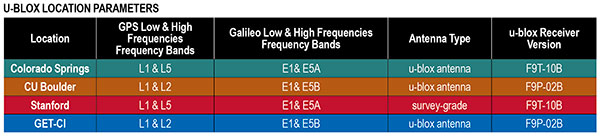
    We collect and analyze a variety of data types and metrics to help identify and characterize jamming and spoofing occurrences. The receiver model we started with, u-blox ZED-F9P-02B, can monitor two different RF bands and many signals, including GPS L1C/A, L2C; GLONASS L1OF, L2OF; Galileo E1B/C, E5b; BeiDou B1I, B2I; QZSS L1C/A, L1S, L2C; and SBAS L1C/A. It has 184 channels, which can be configured to sweep through an array of signals to be monitored. We are also developing monitors based on the recently released ZED-F9T-10B, which is capable of L1 and L5 signal reception. TABLE 1 describes which version of the u-blox receivers each dataset comes from.

    TABLE 1. Locations of u-blox monitor for nominal noise environment characterization and jam/spoof test. (Data: Authors)
    TABLE 1. Locations of u-blox monitor for nominal noise environment characterization and jam/spoof test. (Data: Authors)

    L1 and L5 are the primary frequencies used for aviation, hence a monitor for these frequencies would be more useful for protecting aviation than the F9P, which is only capable of L1 and L2 reception. The available data includes raw measurements such as code and carrier phase, position estimates, power level estimates including C/N0, AGC and spectral power. It also has active CW interference detection. These metrics are all necessary for the consistency checks and power monitoring methods we summarize in this article. Consult our conference proceedings paper for details (see Acknowledgments). By examining all of these signals and measurements, we can observe changes in the RF environment and detect inconsistencies in the received signals.

    Data Logging. The u-blox receiver logs messages in a specific format. The message types important to log are selected based on the desired data. Due to limited bandwidth, we prioritized messages that efficiently include all desired parameters for the interference detection methods we describe in this article. We have used both the u-blox F9P and the u-blox F9T. 

    To characterize nominal noise environments, u-blox receivers were set up at three locations: Stanford University, the University of Colorado (CU) in Boulder, and at the Colorado Springs airport. All measurements from satellites below an elevation angle of 5 degrees were ignored. The results from these locations are summarized below. Results from a jamming/spoofing test sanctioned by the U.S. Department of Homeland Security are presented and labeled with the acronym “GET-CI” (GPS Testing for Critical Infrastructures) in the subsequent discussion. Table 1 describes the parameters of the u-blox receiver at each location.

    Positioning Metrics Development. The nominal error of the single- and multi-constellation position solutions is made by noting the difference between the computed position and the known truth. The inter-constellation consistency check is defined as the difference between the positions computed from two constellations, with no reference to a known truth position. To analyze the nominal differences in the north, east and down (NED) directions, we use the position covariance matrix, R, computed in the least-squares solver, to set a covariance-bound threshold. The covariance for each constellation is assumed independent. We present our results using this threshold in our results sections. 

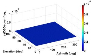
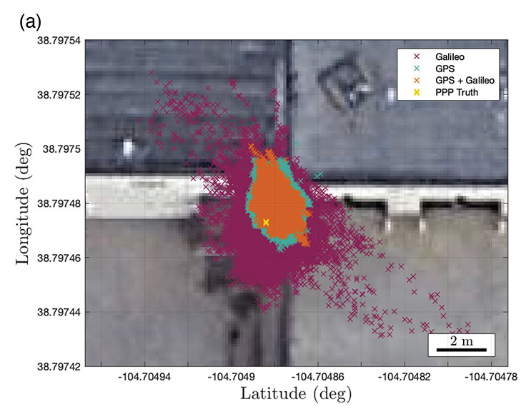
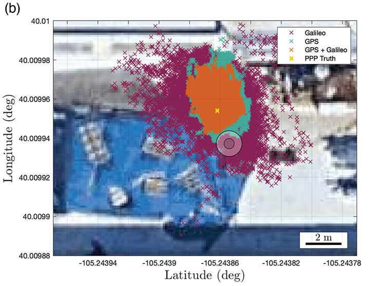
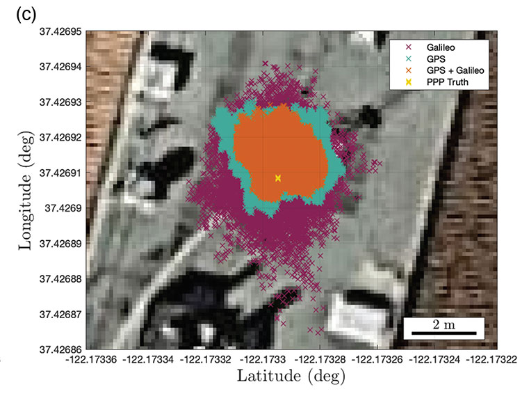
    Our results in FIGURE 1 show that the Galileo position solution variance is higher than the dual-constellation and GPS-only solution. This is attributed in part to the fact that Galileo, while operational, has not filled out all planned satellite slots and therefore has fewer satellites and worse geometry than GPS. 

    FIGURE 1a. Map visualization of the comparison among position solutions computed using only GPS, only Galileo and a combined GPS plus Galileo dual-constellation solution at Colorado Springs. (Image: Authors)
    FIGURE 1a. Map visualization of the comparison among position solutions computed using only GPS, only Galileo and a combined GPS plus Galileo dual-constellation solution at Colorado Springs. (Image: Authors)
    FIGURE 1b. Map visualization of the comparison among position solutions computed using only GPS, only Galileo and a combined GPS plus Galileo dual-constellation solution at CU Boulder. (Image: Authors)
    FIGURE 1b. Map visualization of the comparison among position solutions computed using only GPS, only Galileo and a combined GPS plus Galileo dual-constellation solution at CU Boulder. (Image: Authors)
    FIGURE 1c. Map visualization of the comparison among position solutions computed using only GPS, only Galileo and a combined GPS plus Galileo dual-constellation solution at Stanford. (Image: Authors)
    FIGURE 1c. Map visualization of the comparison among position solutions computed using only GPS, only Galileo and a combined GPS plus Galileo dual-constellation solution at Stanford. (Image: Authors)

    Nominal Noise Results

    Here are some of our positioning and power monitoring results under nominal reception conditions.

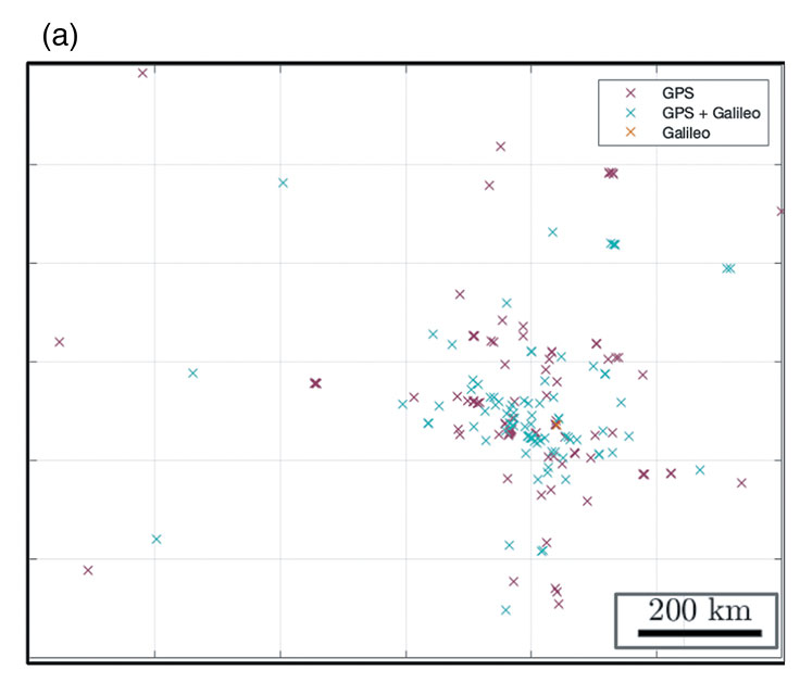
    Positioning. Based on the methods described earlier, we present a selection of our results from the positioning consistency checks. We present several informative visualizations of the error between the computed position solution and the known truth of each u-blox receiver and use the covariance threshold to bound the raw error. The error for dual-constellation, single-constellation and inter-constellation consistency checks are all displayed and compared to one another. The pseudorange residuals and their accompanying chi-squared (χ2) statistic are also evaluated and compared for the GPS and Galileo single-constellation position solutions.

    Positioning Consistency Comparison Maps. From the maps in Figure 1, we observe that Galileo has the highest error, followed by GPS, and then the dual-constellation solution. The map also serves as a method to spatially visualize the tails of the error distribution.

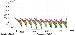
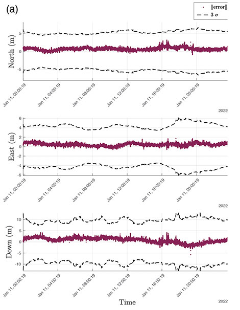
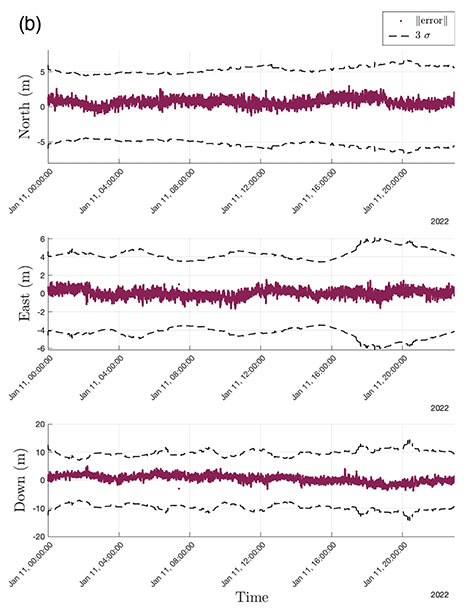
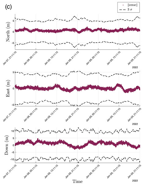
    NED Time Histories. We compare the time history of the dual-constellation, GPS and Galileo position solution error to the three sigma (3σ) covariance bound computed at each epoch (see FIGURE 2). We also compare the GPS vs. Galileo inter-constellation difference to the 3σ covariance bound. The covariance bound is never crossed, indicating that 3σ threshold is conservative for both the error and the inter-constellation difference between GPS and Galileo.

    Photo:FIGURE 2a. Dual-constellation north-east-down error vs. known truth, bounded by a 3σ threshold, at Colorado Springs. (Image: Authors)
    FIGURE 2a. Dual-constellation north-east-down error vs. known truth, bounded by a 3σ threshold, at Colorado Springs. (Image: Authors)
    FIGURE 2b. Dual-constellation north-east-down error vs. known truth, bounded by a 3σ threshold, at CU Boulder. (Image: Authors)
    FIGURE 2b. Dual-constellation north-east-down error vs. known truth, bounded by a 3σ threshold, at CU Boulder. (Image: Authors)
    FIGURE 2c. Dual-constellation north-east-down error vs. known truth, bounded by a 3σ threshold, at Stanford. (Image: Authors)
    FIGURE 2c. Dual-constellation north-east-down error vs. known truth, bounded by a 3σ threshold, at Stanford. (Image: Authors)

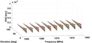
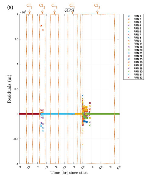
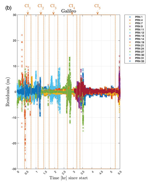
    Pseudorange Residuals and χ2 Statistic Threshold. Pseudorange residuals have a long history of being used as a consistency check between range measurements. As an example, the pseudorange residuals for the GPS position solutions are shown in FIGURE 3, and their corresponding χ2 statistic is shown in FIGURE 4.

    FIGURE 3a. GPS pseudorange residuals at Colorado Springs. (Image: Authors)
    FIGURE 3a. GPS pseudorange residuals at Colorado Springs. (Image: Authors)
    FIGURE 3a. GPS pseudorange residuals at Colorado Springs. (Image: Authors)
    FIGURE 3b. GPS pseudorange residuals at CU Boulder. (Image: Authors)
    FIGURE 3c. GPS pseudorange residuals at Stanford. (Image: Authors)
    FIGURE 3c. GPS pseudorange residuals at Stanford. (Image: Authors)
    FIGURE 4a. GPS χ2 and probability of false alert (PFA) threshold for the nominal noise environments at Colorado Springs. (Image: Authors)
    FIGURE 4a. GPS χ2 and probability of false alert (PFA) threshold for the nominal noise environments at Colorado Springs. (Image: Authors)
    FIGURE 4b. GPS χ2 and probability of false alert (PFA) threshold for the nominal noise environments at CU Boulder. (Image: Authors)
    FIGURE 4b. GPS χ2 and probability of false alert (PFA) threshold for the nominal noise environments at CU Boulder. (Image: Authors)
    FIGURE 4c. GPS χ2 and probability of false alert (PFA) threshold for the nominal noise environments at Stanford. (Image: Authors)
    FIGURE 4c. GPS χ2 and probability of false alert (PFA) threshold for the nominal noise environments at Stanford. (Image: Authors)

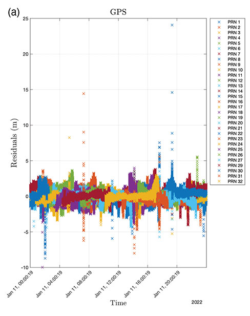
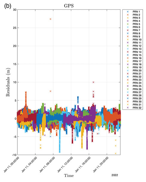
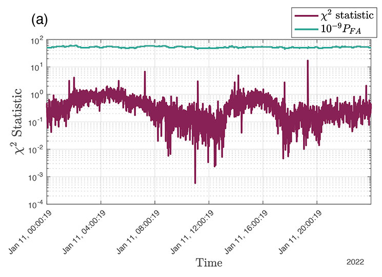
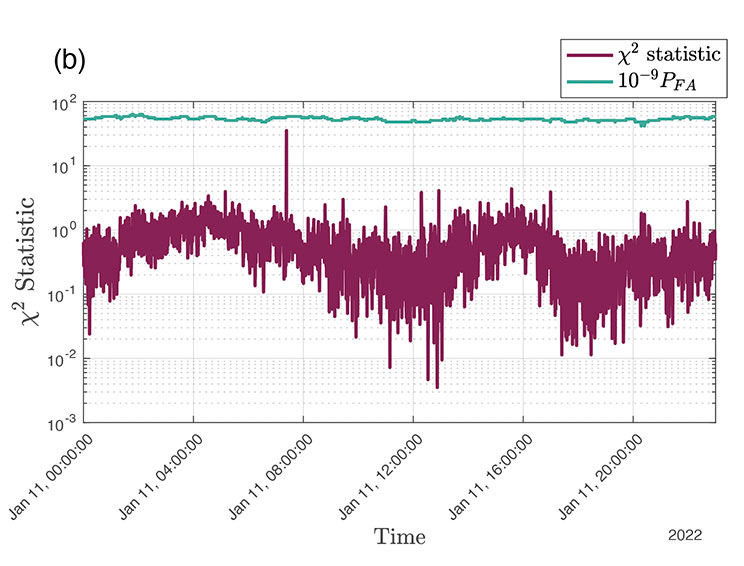
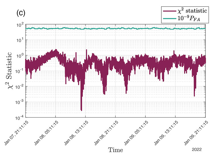
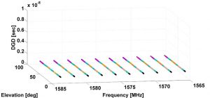
    The χ2 statistic is computed using the finite pseudorange residuals at each epoch, where the degrees of freedom are n − 4, where n is the number of satellites used at that epoch and 4 is the number of variables solved for (x, y, z, and the receiver time offset) when using a single constellation. A p-value is computed using the cumulative distribution function (CDF) of the χ2 statistic, and indicates the probability that the χ2 statistic at each epoch would be greater than the observed value. The statistic is compared to a theoretical 10−9 probability of false alert (PFA) based on the theoretical χ2 and the actual degrees of freedom of each epoch. Very low values for the χ2 statistic, such as those obtained with Galileo, are attributed to regions where very few satellites are in view, thus decreasing the degrees of freedom. Any spikes in the pseudorange residuals are also reflected with a higher χ2 statistic and low p-value, though those residuals are de-weighted in the position solution and ultimately do not trigger the 10−9 PFA threshold or the 3σ threshold, thus indicating that a 10−9 PFA is a conservative threshold. 

    Power Monitoring. For each nominal location with a u-blox receiver, we analyze results from the power-monitoring metrics mentioned earlier. We also observe results from the internal u-blox jamming indicators in a region where a possible RFI event was observed.

    For power monitoring, we analyze spectral power and programmable gain amplifier (PGA) results. 

    For the nominal noise environments, the spectral power, PGA and corresponding C/N0 results indicated no significant anomalies.

    Threshold and Metric Validation Results

    An examination of thresholds and other metrics are important for characterizing RFI.

    GPS Testing for Critical Infrastructure. From a DHS-sanctioned RFI testing event, we identify five regions of interference or spoofing. To identify the interference, we use a combination of the power and positioning metrics as well as the thresholds we developed through the characterization of the nominal noise environments described in the previous sections of this article.

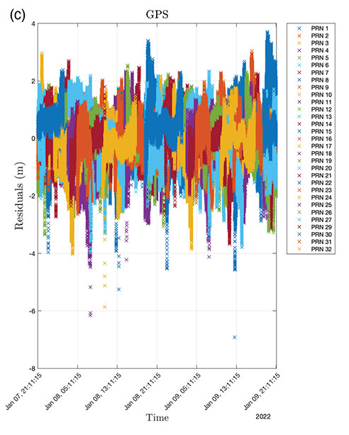
    We use the thresholds and tests we’ve developed to identify regions of spoofing and RFI events (labeled C I1–C I5) in the GET-CI dataset. For ease of comparison, all regions are labeled on plots that display the full 5.5 hours of data collection. All details as to the truth location and time of the test have been removed. C I1 is identified through the power metrics. C I2–C I5 are identified as regions that the NED difference between GPS and Galileo clearly crossed the 3σ threshold in all three directions, as visualized in FIGURE 5.

    FIGURE 5a. Map view of solutions using GPS, Galileo and GPS plus Galileo for the DHS-sanctioned RFI testing event (identifying coordinates and physical features removed). (Image: Authors)
    FIGURE 5a. Map view of solutions using GPS, Galileo and GPS plus Galileo for the DHS-sanctioned RFI testing event (identifying coordinates and physical features removed). (Image: Authors)
    FIGURE 5b. Corresponding log-scale visualization of the GPS vs. Galileo position solution difference in the north-east-down directions. (Image: Authors)
    FIGURE 5b. Corresponding log-scale visualization of the GPS vs. Galileo position solution difference in the north-east-down directions. (Image: Authors)

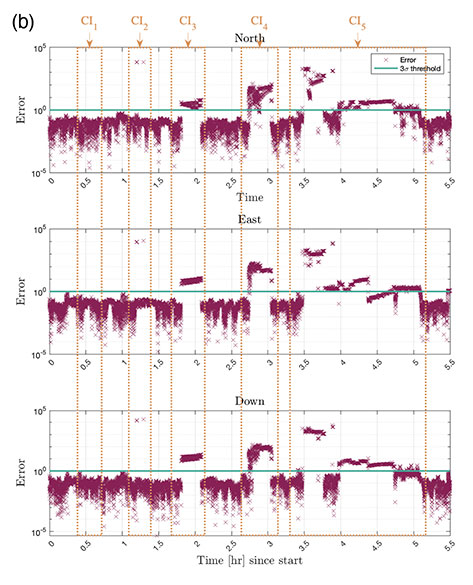
    From our pseudorange residuals, it appears as though the most significant interference events happened on the GPS constellation, as indicated by the high pseudorange residuals that fall into the C I2 and C I5 regions. Using the GPS χ2 statistic and p-value computations, we determined that the regions that crossed the 10−9 PFA threshold line are consistent with the regions of interference identified in Figure 5. The Galileo χ2 statistic, p-values and pseudorange residuals all show signs of possible interference. These regions are explored more in the power monitoring discussion below. 

    Since the GPS pseudorange residuals and χ2 statistic results show more signs of spoofing than the Galileo ones, we explore the Galileo-only position solution. Because the truth position is unknown, we take a point during the non-C I regions and define this as the “truth,” that is, a point in the position solution we believe has not been subject to spoofing. Any references to a truth position are from a position recognized as “truth” through post-processing rather than from a pre-determined and known location.

    The p-values dip in each of the C I regions, but are lowest in regions C I5. Combined with the fact that the pseudorange residuals and NED error are the highest in C I5, we identify this as the region that likely experienced a significant spoofing event. We determined from an outlier at the beginning of the C I5 region (see Figure 5) that even the Galileo constellation is not immune to the spoofing in this scenario.

    To further check the accuracy of our determination that GPS was spoofed, we evaluated the histograms of the Galileo error. With the biggest outlier in C I5 removed, we saw that the error appears relatively Gaussian, with some outliers and possible multi-modal behavior that were also seen in the nominal locations. The variance was higher than was observed at nominal locations, which could be attributed both to the presence of known RFI events, the fact that the nominal noise environment at the RFI event test has not been characterized (that is, it is possible there is a noisier nominal environment at this location), and that the “truth” position was not a known truth but obtained through post-processing of a dataset with increased RFI. Normalized error indicates that the error does not cross the 3σ threshold in any NED direction, further supporting the assertion that 3σ is a conservative threshold.

    Important to note is that the major outlier around T+3.5 hours is visible in the NED plot (Figure 5), but the corresponding histograms do not contain that outlier. This indicates that the covariance also increases at that point. It dictates a need to monitor the covariance bound itself, as well as the positioning error. The NED time history plot and the raw error histograms serve this purpose, since it is clear that if we were to be only looking at the error normalized by 3σ, we would not have found significant evidence of the outlier, since the normalized error barely passes the 3σ threshold. This further supports our methods of combining multiple metrics, thresholds and visualizations rather than relying on a single metric to identify jamming and spoofing.

    From the Galileo solution analysis, we increase our confidence that we have identified the regions with interference. We removed those areas and looked at the GPS vs. Galileo inter-constellation consistency difference. The normalized differences were now mostly within the 3σ threshold, and the raw error displayed some Gaussian behavior and is no longer on the order of the 105-meter error we were seeing in Figure 5. While these regions still have a higher error than nominal conditions and thus still display signs of interference, we are able to use our spoofing analysis to identify epochs in which we should not trust the GNSS. Using times outside those regions, we are able to figure out a reasonable truth position within 20 meters rather than 200 kilometers.

    Positioning analysis using the inter-constellation consistency check is a powerful tool for determining the reliability of a position solution, even when the truth location is unknown. With the power metrics, we can further corroborate the positioning results, as well as find events indicating interference that the positioning metrics were unable to track. 

    FIGURE 6a. GPS pseudo range residuals for position solutions computed using only the GPS constellation. (Image: Authors)
    FIGURE 6a. GPS pseudo range residuals for position solutions computed using only the GPS constellation. (Image: Authors)
    FIGURE 6b. Galileo pseudorange residuals for position solutions computed using only the Galileo constellation for the DHS-sanctioned RFI testing event. (Image: Authors)
    FIGURE 6b. Galileo pseudorange residuals for position solutions computed using only the Galileo constellation for the DHS-sanctioned RFI testing event. (Image: Authors)

    Next Steps and Summary

    Leveraging the raw data collected by u-blox receivers in multiple locations with different nominal noise environments, we have developed the toolsets to do inter- and intra-constellation consistency checks to monitor for jamming and spoofing. Many further observables usable for RFI detection are being recorded by the u-blox receivers. Several power monitoring metrics have been evaluated in a preliminary analysis. The next step is to further characterize metrics such as C/N0, AGC and u-blox internal jamming metrics under nominal conditions. 

    In summary, the tools we have developed so far show that the u-blox receiver will allow for many different consistency checks on a variety of parameters to be running simultaneously. It would be difficult for a spoofer to interfere with all the dimensions we have covered in our detector. Continuously monitoring a wide variety of parameters will increase the chance that we are able to detect interference, thus lowering the chance that a spoofer is able to evade detection.

    Acknowledgments

    We gratefully acknowledge the support of both the FAA Satellite Navigation Team and The Aerospace Corporation under their university partnership program. We especially wish to thank Steve Lewis of Aerospace for his support and guidance throughout the development of this project. This article is based on the paper “Low Cost RFI Monitor for Continuous Observation and Characterization of Localized Interference Sources” presented at ION ITM 2022, the 2022 International Technical Meeting of the Institute of Navigation, Jan. 25–27, 2022. 


    LEILA TALEGHANI recently graduated with her MS degree from Stanford University in aeronautics and astronautics and is now a navigation engineer at Trimble.

    FABIAN ROTHMAIER is a navigation research and development engineer at Airbus Defence and Space in Munich, Germany, and a former a Ph.D. student at the Stanford GPS Laboratory. 

    YU-HSUAN CHEN is a research associate at the Stanford GPS Laboratory. 

    SHERMAN LO is a senior research engineer at the Stanford GPS Laboratory.

    TODD WALTER is a research professor in the Department of Aeronautics and Astronautics at Stanford University. 

    DENNIS AKOS is a professor with the Aerospace Engineering Sciences Department at the University of Colorado, Boulder.

    BENON GRANITE GATTIS is a laboratory assistant and undergraduate student in the Aerospace Engineering Sciences Department at the University of Colorado, Boulder.

  • Antenna pattern uniformity effects on pseudorange tracking error

    More satellites, more constellations, more multi-frequency receivers — they all drive greater achievable accuracy. But they also raise the requirements on GNSS antennas because of the stronger impact that possible imperfections might have in the overall error budget for multi-frequency combinations. This analysis of antenna-induced errors in pseudorange code measurements for different antenna feed types helps identify the advantages and disadvantages of such technologies for precise positioning.

    By Stefano Caizzone, Mihaela-Simona Circiu, Wahid Elmarissi, Christoph Enneking, Michael Felux and Kazeem A. Yinusa, German Aerospace Center (DLR)

    The combination of signals from two frequencies and multiple constellations leads to dual-frequency multi-constellation (DFMC) capabilities, which currently appear to provide improved performance, due to the increased number of satellites available. This leads to better available satellite geometries, but also to the possibility to strongly mitigate ionosphere-related errors, thanks to dual-frequency combination of the ranging signals.

    In such scenarios, the hardware-related errors (from satellite and even more from receiver side) will gain a much stronger weight in the overall error budget and should be tackled accordingly.

    This article focuses mostly on the receiver antenna contribution, leaving the effects due to the satellite and to the receiver for later work. We will show that the choice of the antenna technology (mostly in terms of the number of feeding points) has a strong impact on the pattern uniformity and therefore on the differential group-delay characteristics over the aspect angle. Optimal performance is demonstrated when using more sophisticated solutions, providing a ground for cost/performance analysis to system engineers of specific applications.

    GROUP DELAY PERFORMANCE

    Antenna performance in GNSS application is mostly evaluated in terms of antenna gain pattern, noise figure and group delay for code measurement or phase center variation for carrier phase measurement. Gain and noise figure impact on the signal level available at the receiver, while the group delay is a measure of the delay introduced by the antenna hardware to the different spectral components of the signal. The differential group delay (DGD) is

      (1)

    with φ, f, Az, El being respectively the antenna phase, frequency, azimuth and elevation.

    The DGD variation with respect to frequency and aspect angle (that is, elevation and azimuth) actually poses a problem in precision applications: as a matter of fact, if the group delay were constant for all frequencies and all angles of arrival of the signal, no additional error would be introduced in the position calculation, because the group delay term common to all satellites would be encapsulated at the receiver into a user clock offset.

    However, group delay can change significantly with respect to aspect angle and frequency, contributing in a different manner for each satellite (due to different angles) and for different signals (due to the different spectral components of each signal), therefore finally producing errors in the pseudorange estimation.

    The influence of the DGD on pseudorange measurement error has already been studied in the past and is also taken into consideration in the antenna Minimum Operational Performance Standards (MOPS) for avionic antennas. Empirical studies on the combined effect of antenna group delay and multipath effect on board commercial airplanes have been published recently. However, to our knowledge, the correlation between the antenna intrinsic characteristics (such as gain and phase patterns and smoothness) and group delay behavior has not yet been properly analyzed, leaving a gap in the full understanding of the antenna design impact on the final GNSS receiver performance.

    GNSS antennas can be divided into families, according to their geometry (and the related radiation mechanisms): for instance, spiral, helix and microstrip (patch) antennas are quite common in GNSS applications.They differ in achievable bandwidth, size and ease of manufacturing.

    Even antennas of the same family can provide different performance, mainly because of the number of feeding points, which are the points where the signal is fed into the antenna.

    In order to analyze the relationship between the group delay performance and the antenna properties, we will take into consideration three GNSS antennas of the same family (microstrip patch), having all about half-effective-wavelength size (with the effective wavelength considering the dielectric properties of the substrate material on which the patch antenna is positioned), but with a different number of feeding points. The antennas will be denominated respectively single-feed, double-feed and four-feed antennas.

    The single-feed antenna is a square patch, with truncated corners to achieve circular polarization. On the other hand, the double- and four-feed antennas are square patches, having feeds positioned along their x- and y-axis. The feeds are fed progressively: that is, with same amplitude and 0°–90° phases for the double feed and 0–90–180–270° phases for the four feed.

    Single-feed antennas are representative of lower cost antennas used in mass-market applications, due to their extreme simplicity allowing for low-cost production. However, their performance exhibits strong cross polarization levels and non-uniform patterns over the azimuth. Dual- and four-feed antennas are more complicated to manufacture and need further hybrid circuits to properly distribute the signal between the different feeding points. However, an increase in the feeding points leads to more uniformity in the radiation pattern and lower-cross polarization and can therefore be expected to improve performance.

    Dual-feed antennas are common in applications where a balance between precision and cost is needed, while four feeds are used in high-end applications, such as geodesy and reference stations.

    The antennas under consideration here have been tuned to obtain optimal behavior at GPS L1/Galileo E1 band and have been simulated in an electromagnetic solver (Ansys HFSS), with an infinite ground plane assumption, to resemble the large metallic body frame of aircraft structures.

    The gain patterns of the different antennas at GPS L1 / Galileo E1 central frequency ( f=1575 MHz) are shown in Figure 1. As discussed earlier, the pattern is not uniform over angle for the single-feed solution. On the other hand, the four-feed antenna shows improved pattern uniformity: the pattern has fewer azimuth and elevation variations, with the two-feed solution providing intermediate results.

    Phase patterns for the three antennas are shown in Figure 2. Here again, the one-feed solution exhibits more angular variation than the multi-feed solutions. It is interesting to notice how strong phase variations occur in the same regions where the gain pattern also varies strongly.

    When considering the DGD, the frequency dependence of the phase pattern will have to be taken into account, according to Equation (1). To show the DGD variability with respect to the aspect angle, the standard deviation of the DGD over a 20-MHz bandwidth has been calculated (for each azimuth and elevation angle) and is shown in Figure 3, confirming the better behavior of the four-feed antenna.

    Figure 4 shows the group delay versus frequency and elevation (with different azimuth values being represented by curves with different colors) for the three typologies of antennas: such typology of figure contains all information about DGD variation versus frequency and angle and is first introduced in this article. For comparison, in the RTCA’s 2006 MOPS document for airborne antennas, for the sake of simplicity, either DGD variation versus angle at central frequency or DGD variation over frequency at zenith were considered, hence not fully covering the complete space {Frequency, Azimuth, Elevation}.

    While the single-feed antenna in Figure 4 shows a big variation of the DGD when moving from zenith (that is, Elevation = 90°) to lower elevations, a substantial decrease in the DGD spread is recorded for the four-feed solution, with the dual-feed one having again intermediate results.

    It is worthwhile noticing that the results obtained for the dual-feed solution are in agreement with the current MOPS for L1 antennas (RTCA DO-301), specifying a maximum value of 2.5 nansoseconds (ns) for the group delay spread at low elevations (normalized to boresight, El = 90°).

    The results show how angular variation of the DGD can be related to non-uniformity along the aspect angle (Az or El) and frequency, hence suggesting to use multiple-feed solution for obtaining optimal performance.

    A useful metric to quantify the uniformity of the group delay can be introduced as the Uniformity Indicator for Group Delay (UIGD):

       ( 2 )

    with  being the sum over frequency (Nf  is the number of frequency steps considered) and DGDzenith,n being the value of the DGD at zenith for frequency n.

    The UIGD expresses the maximum variation of the DGD over elevation and azimuth from a reference condition (the DGD at zenith) in the bandwidth of interest, extending de facto the MOPS requirements by considering the whole bandwidth behavior in the whole upper hemisphere.

    The UIGD for the one-, two- and four-feed antennas is respectively 4.18, 1.03 and 0.05 ns, hence effectively mirroring the better pattern uniformity of the four-feed solution.

    The UIGD is a comprehensive metric to describe the DGD uniformity, but needs accurate phase measurement over the entire bandwidth, which may not be always easily obtainable. As a matter of fact, phase can be challenging to measure: some indication of the areas most likely to deliver increased DGD can be found while considering gain patterns, qualitatively providing an easier metric to compare different antennas. In this case, the Uniformity Indicator for Gain (UIG)can be used:

       (3)

    The UIG expresses the maximum value over all elevation and azimuth angles of the standard deviation of the RHCP gain derivative over frequency (in the band of interest), therefore indicating the roughness of the antenna gain pattern in frequency and angle.

    Such a metric does not relate totally with DGD behavior, but serves as an easier metric of pattern uniformity. The UIG for the one-, two- and four-feed antennas is respectively 68.5, 5.7 and 0.3%.

    REAL-LIFE PERFORMANCE AND IMPACT ON ACCURACY

    To evaluate the performance of actual antennas, three prototypes were measured in a Satimo Starlab anechoic chamber at the German Aerospace Center (DLR).

    The antennas under test were:

    • A badly polarized COTS active antenna, having a behavior similar to that of a single-feed antenna;
    • An in-house developed passive antenna with two feeds;
    • An in-house developed passive four-feed antenna.

    All antennas were properly tuned to obtain optimal gain and minimum reflection losses (input reflection coefficient <–10 dB) at L1 /E1 central frequency.

    The measured RHCP pattern for the various antennas is shown in FiGURE 5. The UIGD for these antennas is 0.9, 0.7 and 0.2 ns respectively, while the UIG is 46.6, 38.5 and 9.0%.

    Differential group delay was calculated from the measured phase values and is shown in Figure 6.

    The results are similar to those obtained from simulation and clearly show the improved flatness of the DGD for the four-feed case.

    Moreover, if the measured phase data are fed into an ideal GNSS receiver, able to provide the tracking biases occurring in the pseudorange code measurement for all elevations and azimuths, antenna-effects-only (as weighted by the signal characteristics) will be visible (as in this case, neither multipath nor receiver or satellite imperfections are included in the ideal receiver). The results are shown in Figure 7.

    A substantial decrease in the antenna-induced error is evident as expected when the four-feed antenna is used.

    The differences in performance among different antenna technologies shown here provide valuable insight in the choice of the antenna technology for a specific application, thanks to the better understanding of the impact of the antenna characteristics on the error at pseudorange level. Moreover, they can support the evaluation and definition of antenna requirements and connect them to the expected GNSS pseudorange error, such as during the process of MOPS definition as currently occurring for DFMC systems.

    CONCLUSIONS

    After investigating the effects of pattern uniformity on antenna-induced errors, group delay behavior over aspect angle and frequency has been shown comprehensively for different antenna feeding technologies for the first time. Minimal error in pseudorange measurements is obtained when the antenna has a smooth pattern, with no abrupt variations or nulls/sidelobes both in aspect angle and frequency. Different antenna feeding technologies currently in use for circularly polarized radiation have been evaluated, and the best performing one has been identified in the multiple-feed solution.

    Both a comprehensive and an easier-to-measure metric for group delay uniformity have been identified, providing useful insight for fast comparison of the performance of multiple antennas in terms of GNSS accuracy.


    STEFANO CAIZZONE received a Ph.D. in geoinformation from the University of Rome, Tor Vergata. He is is responsible for the development of innovative miniaturized antennas in the antenna group of the Institute of Communications and Navigation of the German Aerospace Center (DLR).

    MIHAELA-SIMONA CIRCIU received a master’s degree in computer engineering from Technical University Gheorghe Asachi, Romania, and a master’s in navigation and related applications from Politecnico di Torino, Italy. She works on the development of the multi-frequency multi-constellation Ground Based Augmentation System for DLR.

    WAHID ELMARISSI received a Dipl. Ing. in electrical engineering from the University of Applied Sciences, Kiel, Germany. He is responsible for measurement and manufacturing of antennas and antenna electronics at DLR.

    CHRISTOPH ENNEKING received a MSc. degree in electrical engineering from the Munich University of Technology. He conducts research in GNSS signal design, estimation theory and GNSS intra- and inter-system interference at DLR.

    MICHAEL FELUX is a research associate specializing in GBAS integrity issues for CAT -II/III operations and program manager for the research on GBAS navigation at DLR. He graduated in technical mathematics at Technische Universität München.

    KAZEEM A. YINUSA received MSc. and Dr.-Ing. degrees in electrical engineering from the Technische Universität München. He is a researcher at DLR.

  • Google to provide raw GNSS measurements

    Google to provide raw GNSS measurements

    User location takes center stage in new Android OS

    Raw GNSS measurements from Android phones. Yep, they are coming. At Google we have been working with our GNSS partners to give application developers access to raw GNSS measurements from a phone.

    This is really exciting, and marks a new era for our GNSS community. At Google I/O in May, we announced that raw GNSS measurements are available to apps in the Android N operating system, which will be released later this year. This means you can get pseudoranges, Dopplers and carrier phase from a phone or tablet.

    When can you get it? Well, it will take some time to proliferate throughout the ecosystem, but the first phone that will provide raw measurements will be the Nexus phone that we will launch later this year, and then next year you will see new Android handsets start to support it, as it will become a mandatory feature in Android.

    Tutorial. At the Institute of Navigation’s ION-GNSS+ conference this September, Frank van Diggelen and I will teach a tutorial where you can learn to access and use these raw measurements. This will be a hands-on course where you collect, view and process raw measurements. You will leave the class with the data, Google software tools, and the knowledge of how to use them.

    This tutorial is open only to ION-GNSS+ attendees. To register for the conference, visit www.ion.org/gnss/registration.cfm.

    Then, to tailor this tutorial to your own needs, visit this online form and let us know what you’d like us to cover in the class.

    The keynote presentation at Google I/O 2016, held May 12-20 at Shoreline Amphitheater in Mountain View, California.
    The keynote presentation at Google I/O 2016, held May 12-20 at Shoreline Amphitheater in Mountain View, California.

    More from Google I/O

    Finally, I’d like to give you some highlights from Google I/O, the annual developer-focused conference held by Google in the San Francisco Bay Area.

    During the keynote, Google CEO Sundar Pichai made many references to location, context and places. This was really exciting to see. We are innovating and working on a lot. It is amazing, even to me, after more than 13 years in the field of location, arriving at Google just under two years ago, to see how location and a user’s context are at the center of our connected world.

    At Google, we are exposing as much as we can to the ecosystem so that innovation can thrive around us.

    Sundar Pichai’s keynote address shows that user’s location is at the center for the knowledge graphs that we are building.

    Conversational examples were shown on Google Assistant and on how it can be used to get things done in the world. Sundar spoke on how location and context are the key to this future, noting that a user standing next to a famous sculpture can simply ask: “Who designed this?”

    All Google I/O talks from the Android Location and Context Team can be found at these YouTube links :

  • Research Online: HF beacon navigation, inertial sensors and GNSS-INS integration

    Photo: HF Beacon NavigationHF Beacon Navigation

    Navigation using High-Frequency Ground Beacons and Ionosphere Model Corrections, by Yoav Baumgarten and Mark L. Psiaki, Cornell University.

    A new navigation concept relies on passive one-way ranging using pseudorange measurements of high-frequency (HF) beacon signals reflected off the ionosphere.

    This is being developed as a possible alternative to GNSS positioning and timing services, with benefits in costs and system redundancy. The HF signals are transmitted from ground-based beacons, traveling from known locations to the unknown user equipment (UE) location along ray paths that reflect off the Earth and the ionosphere. If a set of beacon signals reaches the UE receiver with sufficient geometric diversity, then the three-dimensional position and the clock offset of the receiver can be determined.

    Presented at ION GNSS+ 2015.

    Inertial Sensors

    Dynamic Stochastic Modeling of Inertial Sensors for INS/GNSS Navigation, by M. Wis, Deimos Space, Spain; Ismael Colomina, GeoNumerics, Spain.

    Researchers performed a series of experiments with a low-cost inertial device rigidly attached to a navigation-grade reference IMU and found a direct relationship between the low-cost IMU errors and the high-order dynamics. Preliminary results suggest an approach of low-cost sensor modeling that might help reduce some of the errors inherent to the dynamics applied to the sensors.

    Presented at ION GNSS+ 2015.

    GNSS-INS Integration

    Quasi-Tightly-Coupled GNSS-INS Integration with a GNSS Kalman Filter, by Bruno Scherzinger, Applanix Corporation, Canada.

    This method, intended for integration of an existing GNSS navigation engine into a GNSS-INS closed-loop configuration with little/no modification of the navigation engine, uses a range measurement model matrix typically used to compute dilutions of precision (DOP) to identify the observable subspace in the time-space frame generated by the available satellites and project the loosely coupled INS-GNSS Kalman filter position measurement into this subspace.

    Presented at ION GNSS+ 2015.