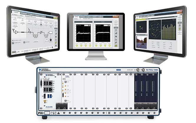
Averna, a global test and quality solutions provider, announced that through existing partnerships, real-time GNSS simulation and satcom signal generator toolkits will be available for the RP-6500 RF record and playback platform, making the RP-6500 an all-in-one solution to support advanced satellite navigation applications.
Averna is exhibiting at Booth #518 during ION GNSS, Sept 26-27, at in Miami, where the company will be demonstrating the RP-6500 Wideband Record & Playback system.
The RP-6500 platform can record and playback up to 500 MHz of RF spectrum from 9 kHz to 6 GHz, as well as simulate all common GNSS signals (BeiDou, Galileo, GLONASS, GPS, and QZSS). The system can also generate Satellite communications signals (DVB-S and DVB-S2).
The robust system fits into a car trunk for driving/recording applications, and syncs with both a GPS and Averna’s DriveView software, for synchronized location and video capture that is time-aligned with your data, the company said. Preloaded with RF Studio, powerful RF record/playback software for capturing real-world RF spectrum, including GNSS, radio, video & location data. A state-of-the-art workflow tool, the RP-6500 Series lets you quickly set up your recordings, add contextual data, visualize weak signals, and analyze your collected RF environments to validate and fine-tune your designs and products.
To learn more about the RP-6500 wideband RF Record and Playback, visit www.averna.com/RP-6500
“We’re extremely happy to add new testing capabilities to our RP-6500, an advanced solution for the design validation of Satellite Navigation systems,” commented Jean-Lévy Beaudoin, vice-president, Platforms & Innovation, R&D for Averna. “The RP-6500 is a complete RF Record and Playback platform–it’s been designed and built from the ground up to be all-in-one.”
Key features and benefits
easy-to-use RF Studio user interface
500 MHz-wide instantaneous bandwidth
covers most common wireless protocols from 9 kHz to 6 GHz
multi-constellation and multifrequency GNSS Simulator
supports SATCOM protocols for Satellite Set-Top Box testing
high dynamic range (14 bits, >80 dB)
form factor allows rack mounting or car trunk portability.
Averna and Skydel Solutions will be showcasing their latest GNSS technology simulation products at The Institute of Navigation (ION) GNSS+ conference, giving show-goers the opportunity to see the RP-6100 in action.
ION GNSS+, taking place Sept. 14-18 in Tampa, Fla., is the 28th International Technical Meeting of the Institute of Navigation’s Satellite Division and the world’s largest technical meeting and showcase of GNSS and related technology, products and services.
The companies will be presenting at Booth #100 in the Exhibit Hall, meeting attendees and discussing their latest innovations in GNSS receiver validation, among other topics. They will also be demonstrating two new GNSS solutions:
RP-6100 Multi-Channel RF Record & Playback: The RP-100 for RF application testing allows users to tecord real-world signals such as GNSS, HD Radio, LTE and Wi-Fi — plus impairments — to significantly advance projects and harden product designs.
GNSS Simulator: New from Averna’s partner Skydel Solutions, this innovative and cost-effective simulator is entirely software driven. It’s a perfect fit with the RP-6100, Averna said, enabling users to test corner cases and future events with a real-time GNSS solution.
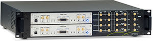
Averna RP-6100 record and playback solution. (PRNewsFoto/Averna)
Averna has launched an RF tool offering high-performance record-and-playback and real-time simulation in one platform.
The Averna RP-6100 series is a self-contained, record-and-playback solution for RF application validation. It can capture all GNSS bands, as well as HD Radio, Wi-Fi, LTE, radar, and cognitive radio — plus impairments — to significantly advance RF projects and harden product designs. The RP-6100 series features up to four channels, 160 MHz of recording bandwidth, tight channel synchronization, an extended frequency range of 10 MHz to 6 GHz, and 14-bit resolution.
The RP-6100 can also be equipped with Skydel Solutions’ software-defined, real-time GNSS simulator, which delivers easy setups, integrated maps, dynamic scenario creation, high precision and tight parameter controls to enable highly repeatable simulations of current and future GNSS conditions, as well as corner cases.
Features include:
Frequency range of 10–6000 MHz, covering all GNSS bands, plus HD Radio, WiFi, LTE, and more
Multi-channel (1-4): Up to 160 MHz of bandwidth at 14-bit resolution (< 1 Hz)
3.8 TB SSD storage or 16 TB HDD storage (for up to 22 hours of recordings)
Preloaded with RF Studio software for quick setups and in-depth analysis
Four models: RP-6120 (2 ch.), RP-6120P (2 ch. portable), RP-6120D (2 ch. desktop) and RP-6140 (4 ch.)
Optional real-time Skydel GNSS Simulator for complete GNSS corner-case/testing scenarios
“We are very excited to partner with Skydel Solutions as a way to continue to provide our customers with the latest technologies and products,” said Benoit Richard, VP of Innovation & Strategy at Averna. “Their technology maps perfectly with our portfolio of RF instrumentation solutions, which empower device manufacturers to efficiently generate, record, simulate, analyze, and play back all common radio, video, and navigation signals, ensuring complete test coverage and the highest quality for their RF products.”
“Today, Skydel is proud to introduce its software-defined GNSS Simulator, running in real-time Ettus and NI USRP hardware,” said Stéphane Hamel, co-founder and CEO of Skydel Solutions. “We are also very pleased to announce that our GNSS Simulator can be combined with Averna’s RP-6100 Series. These technologies complement each other perfectly, making the combined solution the ideal platform for high-performance design validation of RF and GNSS devices.”
The design and verification of a new class of portable wideband record-and-playback system considers the relative merits and limitations of both simulator and record/replay approaches. The authors also discuss the benefits of the different test approaches to the development and characterization of various GNSS receiver types.
By Steve Hickling and Tony Haddrell
As new GNSS systems become available, and users take receivers to ever more challenging environments, the need for repetitive and repeatable testing during development grows ever stronger. Simulators have traditionally demonstrated performance and repeatability in the laboratory environment, and this approach remains the only option for planned signals not yet broadcast from space. However, this approach is becoming more complex as the number of GNSS signals and their reception environments increase.
Another way of testing receivers is through field trials. This allows investigation of conditions difficult to simulate, such as multiple reflections and interferers. These environments, however, are time-varying, and thus not repeatable in the true sense. Therefore, proper comparisons can only be made by assessing all competing receivers in the same trial, and any performance anomalies seen cannot necessarily be tracked down by returning to the same location at some point in the future. Furthermore, developers would like to see for themselves any such anomalies and try to understand and correct them, but it is not always desirable or practical (and certainly not economical) to put development engineers in locations scattered all over the globe.
To tackle this problem, GNSS signal record-and-replay capability is gaining acceptance as a practical tool for recording a signal environment at a single point in time and replaying at will. In real terms this means a device must receive the radio signals from the GNSS satellites, reduce them to a form suitable for storage, and then recreate signals from the stored data in a manner that makes them look completely real to any receiver under test or development.
Some receiver manufacturers developed their own capability to do this. Early devices were of necessity restricted in the signals they could handle and store, limited both by budget and available technologies. The basic problems are the amount of data to be stored in real time and the ability to recover it in real time. Even the GPS L1-only low bandwidth C/A code requires at least 2 Mbytes per single second of recording, or more than 100 Mbytes per minute.
Fortunately, with digital storage technology advances, we can now make use of higher storage capacities (1 TByte of storage is readily available at reasonable cost) and also higher write/read bandwidths (100 MBytes per second is realistic). All we need is some hardware and a processor that can handle the data rates.
Once we have our wanted signals reduced to some form of digital representation, we can simply store and retrieve them at will, handling the recordings as simple, if somewhat large, data files. This allows file distribution between equipments, and a split between making the recording in the field and replaying it in the laboratory. In fact, many manufacturers have dedicated field recording teams who send the files back to the engineers interested in the signal environments.
Replaying the signals is in some ways similar to generating simulated signals. In both cases, the starting point is digital data, on the one hand recorded in the field, on the other hand calculated by mathematical algorithms using the scenario specified in the simulator. In both cases the signal is created by generating radio frequency (RF) carriers and modulating them according to the GNSS signal formats.
Contrast of Two Approaches. None of the characteristics of the record/replay device replace the functionality of the simulator; in fact, both are valid tools for development and testing. For instance, it is not possible with a record/replay device to manipulate individual satellite signals, nor to introduce specific errors in the radio signals. Equally, it is not really possible with a simulator to recreate a particular physical environment made up of many reflected signals, jammers, manmade noise, and moving scenery. With a simulator, the user has control over the power of the received satellite signal, whereas in the recorder the entire signal-to-noise ratio observed at the point of reception has been recorded, and the user can only control the amplitude of the entire noise plus signal.
Permanent Signal Monitoring
One other aspect of raw signal recording lies outside the receiver testing topic, but is of interest for GNSS signal monitoring. It uses the ability to record GNSS signals all of the time, in this case from a good signal environment, and then to retain any time spans where an anomaly in the signals has been detected by a monitor receiver. This is comparable to recording security CCTV pictures, where we expect nearly all of the resulting files to be redundant, but can retain the interesting bits to replay over and over for further analysis. For example, if it is known that a given timing receiver installation suffers periodic loss of lock, it is possible to make a recording using the loss of lock to signpost the interesting region in much the same way as a reverse trigger on an oscilloscope.
Limitations and Compromises
The sheer function of recording GNSS signals off-air has some built-in limitations. First, the signal recorded represents only a snapshot of the environment, although numerous recordings can be made at, say, busy and quiet times, day and night, etc. This is really a reversal of the “non repeatability” aspect of measuring performance in a particular location. In the recording sense, we only get repeatability, with no guarantee that the scenario captured represents worst case conditions. Thus, going back to the location in the future may or may not provide similar results.
In addition to this, there are some signal processing aspects that limit the fidelity of the replayed signals. The first is that any recorder must have an external GNSS antenna and a GNSS receiver front-end built in, and this combination will receive both the satellite signals and thermal noise. The level of the noise is much higher than that of the signals if we don’t do any correlation related processing, and the receiver will contribute some more noise of its own (the noise figure of the system). The second aspect is that in downconverting the radio signals to a usable frequency for sampling and storage, the recorder must use some frequency reference of its own, which will contribute some frequency uncertainty and some phase noise (or jitter on the frequency). The final aspect is the digitization of the downconverted signal to get it into a suitable form for manipulation and storage. Since we are essentially sampling noise here (with the GNSS signal buried in it) we need to look at fidelity in reproduction of the noise during playback, and the effect of any signal (a jammer or interferer) that is above the amplitude of the noise. In analyzing this last aspect, we may include the effect of any automatic gain control (AGC) used to present the correct amplitude signal to the analog to digital (A2D) converter.
A New Simulation Requirement
We wanted to create a much more comprehensive and flexible device than hitherto available, going part way towards the much more general (and expensive) instrumentation recorders that are currently the only alternative.
The requirement is for a flexible, self-contained device that can be easily carried or transported for recording purposes, so having an internal battery and built-in control functionality, and simultaneously a device that fits neatly into a networked and externally controlled laboratory environment.
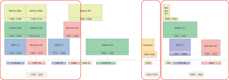
The first approach was to cover all of the possible GNSS frequency bands, although as more are added with time, we realized that this needed to be moderated somewhat. So the product covers L1, L2, L5 and their derivatives for the differing GNSS systems GPS, GLONASS, Galileo, and BeiDou, and also the Inmarsat commercial band to cover the proprietary augmentation signals used by many high-accuracy receivers (see Figure 1, red outlines).
FIGURE 1. Frequency bands, outlined in red, supported by the new record-and-replay device.
The next decision was what bandwidths to allow at each frequency, and how much of this bandwidth could be covered at once. The limitations here are driven by the data storage requirements of the signals being recorded, and the speed that they can be written to disk. The resulting solution allows bandwidths (BW) of up to 30 MHz at each frequency, and any three such bandwidths to be recorded at once. Physically, this is implemented with three channels with the ability to record any of the available frequencies or bandwidths. The user has, therefore, flexibility to set up recording for his particular needs, which may be just L1 covering BeiDou, GPS, Galileo, and GLONASS, or an L1,L2,L5, combination for a survey type application.
Of course, there are always requests for more capability, and we envisaged early on the ability to stack two devices to give six channels of 30-MHz BW for recording, say, GPS/Galileo and GLONASS at L1, GPS and GLONASS at L2, Galileo/GPS at L5, and an Inmarsat data carrier. See later for how this is achieved.
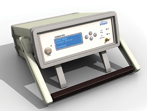
The whole product has to fit in a portable box with enough battery power for more than one-hour field campaigns, and also be capable of running from mains or vehicle power. The associated antenna needs to cover all of the frequency bands. Figure 2 shows the end result in its standalone configuration.
Figure 2. Portable solution for recording.
One additional requirement was placed upon the design, and that is the ability to record and replay non-GNSS data simultaneously with the GNSS signals, and reproduce them, if desired, in synchronism with the replayed signals. This allows time ticks, events, assistance data, sensor data, or even video to be stored and replayed along with the raw signals.
Architecture and Implementation
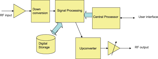
The new record-and-replay device uses a fast computer running the Linux operating system as its control center and storage/retrieval engine. Dedicated hardware is used to format or recover the raw data, and this has access directly to the computer bus to minimize the delays in writing or reading the mass storage, which in this case is a solid state hard drive (SSD). The overall architecture is shown in Figure 3.
Figure 3. Concept-level architecture.
The signal recording capability hinges around the RF planning, which has the task of supplying the necessary flexibility without adding more than minimal signal degradation.
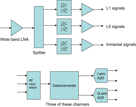
For the RF functionality, the device contains a broadband front end and a three-channel RF amplifier (L1, Imarsat, and L2/L5), filtering the signal down to reasonable bandwidths for later downconversion. Three independent channels of downconversion to baseband I and Q analog signals have access to any of the RF channels and are based upon satellite TV technology architectures. The downconverters have baseband filters that can be commanded to a desired bandwidth by the control processor. This allows the use of narrower bandwidths where possible, allowing more recording time for a lower sampling rate. The baseband signals are sampled at 10 MHz or 30 MHz, paying attention to the Nyquist requirements for pre-digitisation filtering. Two bits for each of the I and Q signals are utilized for packing into the recorded file format. Figure 4 shows the arrangement.
Figure 4 . The RF architecture.
At this stage any additional synchronous data to be recorded, such as truth or assitance data, is inserted into the bit stream, and the data from all the channels in use is combined in a pre-determined format. Dedicated hardware is used for this, and large data buffers are provided to alleviate bottlenecks in sending data to the disks. Each file has an associated definition in a header, and contains synchronization data to allow the device to set up the replay path and recover the data bits in order to reproduce whatever combination was recorded. Note that resulting data files are given the same extension, regardless of content. Data files can be very big (at maximum bandwidth we record about 2.7 Gbytes per minute) and may be difficult to handle once recorded. To assist with this, the device has a second, removable SSD on board, allowing recorded files to be simply popped out of the caddy and shared with another device, or even mailed or couriered. The RF path for the replay consists again of three independent channels, able to generate any of the supported frequencies and modulate upon them the original signals recovered from the stored file. Once again, dedicated hardware and large buffers are needed to unpack the files and send the RF data to the correct channels or to the synchronous data outputs in the case of recorded digital data, as determined by the file header.
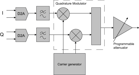
The data representing the recorded RF is converted back to analog form and filtered before being applied to modulators which regenerate the original channelized signals. Each channel has a programmable attenuator to “level” the amplitude, and the three channels are then combined together before passing through a common attenuator to provide user control over the replayed carrier to noise ratio (C/N0). Figure 5 shows the upconverter arrangement.
Figure 5. An upconverter channel.
All frequencies created within the device need to be traceable to a common reference. In addition, this reference needs to be at least as good as the reference in any receiver to be tested, since both its offset from true frequency and its rates of change will be superimposed on the replayed data. Many commercial-grade GNSS receivers (such as those used in mobile phone) are specifically designed to cope with poor oscillators, for instance a low-grade temperature controlled crystal oscillator (TCXO), whereas more professional receivers may expect a couple of orders of magnitude better performance. We decided, therefore, to include an ovenized oscillator (OCXO) for use both in record and playback modes. One challenge presented by this decision is that the oven is necessarily thirsty for power, and therefore a bigger battery is needed than would otherwise be the case.
The OCXO used is a 10.23-MHz component, thus allowing direct generation of the wanted GNSS frequencies using integer ratios and avoiding as much phase noise as possible in the various RF channels. A dedicated phase locked loop (PLL) generates a reference for output to other devices, and a 10-MHz input connector is provided to lock the OCXO to an external reference. These capabilities are utilized when combining two such devices, since we must have the same frequency reference in each. Apart from locking the two oscillators together, this configuration also needs time synchronization between the sampling in both devices, and this is achieved via an additional cable connected between the accessory connectors. Once time and frequency synchronized, the devices behave as a single six-channel unit, using external RF splitter/combiners for the RF connections.
Design Challenges
RF Total Bandwidth. The GNSS bands covered by the device range from the L5 band to the GLONASS L1 band, a total range of 480 MHz allowing for signal bandwidths. Table 1 shows the relevant bands.
Whilst the RF front end must be wide open to this range, assuming the use of a single RF input port, it is obviously necessary to provide bandwidth narrowing by filtering as soon as possible, to exclude jammers or carriers using the space between the GNSS bands, and to avoid the sheer noise power overwhelming the RF circuits. Examination of the supported GNSS services shows them essentially packed into two clusters of frequencies, which provide a convenient way of filtering down the RF input into two RF “channels.” This gets the total bandwidth down to about 180 MHz. Figure 1, the opening graphic for this article, shows the groupings. Beidou B3 and Galileo E6 are currently out of scope for this product, but will be supported in a later version.
The Inmarsat-supported signals are assigned their own RF path, since their structure is data modulated carriers, usually with low SNR. Elsewhere in the Inmarsat band there are more powerful carriers supporting comms traffic, which can “grab” the AGC and therefore cause loss of SNR during the digitization process. Hence this band is processed though its own RF path, maintaining as low a bandwidth as possible consistent with the frequency allocations of the various (proprietary) GNSS augmentation data carriers.
Tradeoffs. Throughput of the recording or replay paths is the performance limitation of the current architecture. Thus a lot of discussions and simulations concerning possible bandwidth, sampling rates, and bit depth tradeoffs was undertaken at the outset of the design. In addition, we needed to decide whether to sample signals at an IF frequency or at baseband. Trials were conducted to determine the real rates of disk access, which are different to the often quoted write and read speeds of computer interfaces.
The results of the trials and simulation led us to adopt a maximum average data rate to/from the storage system of 50 Mbytes/second, this being shown to be available over a period of many hours. Actually, at this rate we fill up a 1-Tbyte disk in about five hours.
To service the GNSS signal bandwidths of interest, again there are two groups of signals. This time we are looking at either the commercial signals (“open service signals” in some systems’ parlance) used by consumer-type receivers, which are relatively narrow band, and the military, high-accuracy, or resilient signals of interest to surveying and precision applications. Therefore, we offer two sampling rates, approximately 10 and 30 MHz, to avoid building large files where more than half of the bandwidth was of no interest to the user.
Next, we have to look at bit resolution. Given that we have generally a noise-like signal with Gaussian characteristics, if we were looking at digitizing at an intermediate frequency (IF), it can be shown that a 2-bit analog-to-digital converter (A2D) would be sufficient to keep the digitization losses to less than 1dB. Obviously, the fewer number of bits we need to store the better, commensurate with achieving the performance targets.
Frequency planning for all of the possible frequencies and bandwidths of interest is a complex task. The requirement here was to downconvert each signal of interest to a low IF suitable for digitizing, whilst having control of the bandwidth to eliminate unwanted signals and fulfill the Nyquist criterion. In addition, we wanted each channel to be isolated from the others even when the replay path involving the generation of the IF carriers was considered.
We therefore decided to downconvert to baseband for each channel, to avoid cross-contamination via the various IFs that would have to be generated for replay. In other words, we adopted an IF of zero Hz. This in turn means that the final bandwidth-determining filters are at baseband, and can readily be controlled by software means rather than having to switch RF paths. By downconverting into quadrature baseband channels, all stored signals are at the same (zero) IF, and crosstalk and imaging during upconversion is avoided.
Thus the A2D architecture of 2 bits in the inphase (I) and 2 bits in the quadrature (Q) arms of the downconverted signal was adopted. Doing the calculation in terms of stored data, we see that we can operate three channels inside our target storage bandwidth, with a margin left for other features such as storing video at the same time.
For 30M samples per second (SPS), each channel has 4 bits or 0.5 bytes
Therefore, for three channels the storage bandwidth is 0.5 * 3 * 30 MSPS, or 45 Mbytes/s
To keep the optimum A2D characteristics, the AGC is designed to adjust the signal amplitude at the converter to give a Gaussian response to the four states determined by the two bits in each arm. The AGC operates independently in each channel. Figure 6 shows the final architecture for the device in block diagram form.
Figure 6. Final architecture.
Real-Time Data Handling. Storage and retrieval of the digitized signals is carried out by dedicated hardware connected to the RF downconverter, the playback upconverter, and the main computer that “owns” the storage media. Large buffers allow the storage media to lag (record) and lead (playback) the real-time signals in time, and to take short breaks for housekeeping functions. Data is packed into a binary file according to a pre-determined sequence, which in turn is set by the number of channels and bandwidths in use. A file header is generated which contains all of the information necessary for reconstructing the data streams for replay. A synchronization sequence is added at the start of the file to allow recovery of the correct bits for each channel and each baseband quadrature arm, and to the correct timeslots for each component. Destroying the correct time reproduction is the most likely issue to cause faulty replay in any record/replay device. GNSS receivers don’t like discontinuous or slewing time!
This approach also allows the insertion of external digital data into the file. Providing the data processing hardware is aware of the individual bits into which this data is placed, digital data recorded at the same time as the raw signals may be regenerated synchronously during replay. Thus any data that is applied to a receiver in a real time trial can be available for the same trial any time after the event. Two streams of synchronous data can be recorded per channel potentially making six serial data streams per chassis available.
User Interfaces
A final challenge presents itself in the case of user interfaces. Although the operational options of the device are quite complex, there is a requirement to be able to capture field data with just the equipment itself and any necessary antenna setup. Consequently, the product has a display and control keys implemented on the front panel, allowing the user comprehensive access to the internal functions using a menu system and scrolling displays. Alternatively, for operation in a lab environment, a network connected user interface is specified, and this requirement is supported by a webserver running on the main processor in the device. Thus, simply opening a web browser and connecting to the device’s IP address allows full functional control.
In addition, connecting a mouse, keyboard, and monitor to the device allows access to the main processor, allowing the running of scripts thus providing full control of replays and receiver functions for running continuous tests in an automated laboratory environment. Using this approach, receiver modifications can be tested over many scenarios and locations many times each, to provide statistically relevant results, without taking up operator time. Remote monitoring is possible using the webserver.
Performance Testing
A range of tests and trials have been carried out to verify that the product meets its specifications, and to measure the performance in a number of real life scenarios.
Repeatability, Degradation, Attenuation. The first and most obvious thing to explore is the effect of the record and playback on signal-to-noise ratio. Since the RF circuits add some noise to the signal recorded, we would expect some degradation to take place here. Also, during replay, the receiver under test adds more noise, depending on its noise figure, although this should be the same as would be added when using “live” signals. Many receivers adjust for their noise figure when reporting C/N0 numbers (C/N0 is a signal to noise measurement normalized to a 1-Hz bandwidth and is the standard reported measurement for most GNSS receivers). However, by replaying back the recorded signal and noise at a higher level than would have been received in “live” conditions, we can eliminate almost all of the degradation. In live versus replayed tests for individual satellites using a JAVAD receiver, which allows us to test all of the supported bands and constellations, we found that replay is possible within ±1 dB of the original live signals. Replayed signals were about 10 dB above the original recorded level to achieve this, effectively swamping the receiver’s noise contribution.
An interesting aspect of controlling the C/N0 this way is the ability to attenuate the replayed signal and, therefore, increase the contribution of the test receiver’s noise figure. Thus, although the recorded C/N0 hasn’t changed, we can attenuate the replay level and use the receiver to add noise.
This process is not linear, and we obviously have to remove nearly all of the 10-dB excess to get started. The device keeps a table of attenuation vs C/N0 reduction, allowing the user to simply dial up the required C/N0 loss. Since this depends on the receiver noise figure, effects may differ slightly from receiver to receiver. Usefully the table is user definable allowing tailoring to a specific receiver.
Losses from Phase Noise, Other Factors. This category of degradation is more difficult to quantify, since the effects are on tracking and therefore range and phase measurement rather than signal to noise ratio. One way of looking at this is, therefore, to establish the positioning performance during live and replayed sessions, and measure the differences. This has some complexity, though, since putting the same signals into a receiver multiple times yields differing performance each time, meaning that we have to use some statistical analysis. Of course this isn’t possible on live signals, and is one reason why repeatable replayed signals are so important in developing GNSS receivers. Another aspect is the fact that some of the effects are differential among frequency bands (filter delays, for instance) and across bands as well (group delay) and also occur in the receiver under test, which will have been calibrated to mitigate its own contribution.
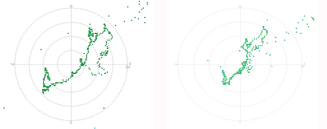
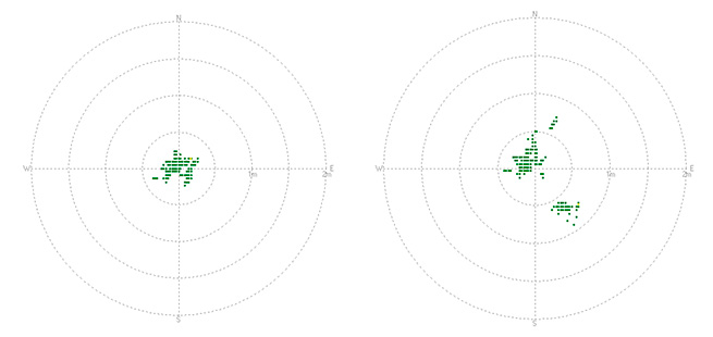
Figure 7 shows a comparison of static positioning for live and replayed signals using only GPS L1 and a 10-MHz sampling rate with an ST-Ericsson receiver, whilst Figure 8 is from a JAVAD receiver using all possible signals in live mode and GPS L1/L2 and GLONASS L1 in replay. In both cases the degradation is within 1 meter always, and much less than this when statistically analyzed.
Figure 7. Static position GPS L1 comparison: live left, replayed right.Figure 8. GPS L1/ L2 with GLONASS L1 comparison.
Another opportunity to measure the effects is to run a zero baseline phase solution, whereby the receiver is used as the “base station” when receiving live signals which are simultaneously recorded. During replay, the same receiver is used as the “rover” with RTK corrections coming from the previously captured live session. In this setup, therefore, we are really only measuring differences in the replayed and live signals, and the usual measurement limitations of the receiver.
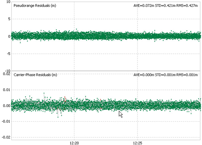
Figure 9 shows the results of one such test, with the pseudorange and carrier phase residuals plotted. This was carried out using two devices in master/slave mode recording GPS L1, L2, L5, and GLONASS L1, L2. As can be seen, the residuals are within “normal” expectations and are measured as 0.42 m RMS for the pseudorange and 1mm RMS for the carrier phase.
Figure 9. Residuals from zero baseline replay.
Drive Test
One of the most common uses for the recorder is to capture the signals at a particular time in a chosen “difficult” environment, A number of representative trials were carried out and we were able to demonstrate consistent results and repeatability. In some cases, the replayed signals yield better performance than live ones, which of course is possible given the differing receiver responses per signal run.
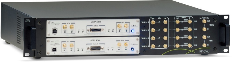
Also, the more times a receivers sees the same time span, the more ephemeris and iono data it can build up, especially true of built up areas where data acquisition is difficult. Figure 10 shows a small section of the City of Coventry in the UK, where the green trace is the “live” plot and the replayed one is in orange. Much of this route is under roads or buildings.
Figure 10. Live and replayed drive around in Coventry.
Dynamic Range and Fidelity
When jamming signals are introduced, the dynamic range comes into play. The earlier discussion of the 2-bit I and 2-bit Q architecture is tested here as the performance of the AGC and A2D is critical in maintaining the fidelity of the GNSS signals in a jamming environment. Note that we are not addressing deliberate jamming here, any “controlled” jammers can be added with an RF mixer at replay. Instead, we are concerned with the everyday jamming environment encountered just about everywhere electronic equipment is deployed.
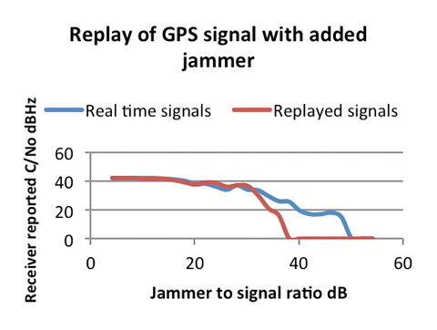
A test was carried out to determine the dynamic range of record/playback paths. A simulator was used as a GPS L1 signals source, and progressively larger jamming signal added via an RF power combiner. The resultant C/N0 in a test receiver was plotted using the live signals which were recorded at the same time. A subsequent replay of those signals was then plotted on top of the original C/N0s. The result is in Figure 11.
Figure 11. Results of the increasing jammer test.
As can be seen, with low jammer powers the real-time and replayed C/N0s track very closely. The ST-Ericsson receiver we used has some signal processing mitigation built in, and so only shows slow degradation as the jammer power is increased. In the real-time run, it was able to track satellites with the J/S ratio greater than 44 dB (and therefore >25 dB above the noise)
On the replayed line, we see the dynamic range limitations start to dominate the replayed signal when the J/S reaches about 30 dB, or 11 dB above the noise, which aligns well with the theoretical analysis of the digitization strategy. This range is sufficient for most environments encountered in real tests.
In Use and Additional Capabilities
With so much flexibility we find that users have a diverse range of applications for the device. These range from multi-constellation usage at L1 only, allowing BeiDou, Galileo, GLONASS, and GPS to be captured, to full six-channel recordings using GPS, GLONASS, and Galileo at L1, L2, and L5 along with an Inmarsat-based assistance channel. For the first time in this class of device, recording of the “military” bandwidth signals is possible. User feedback has been favorable, especially since the unit opens up new capabilities for receiver development and testing.
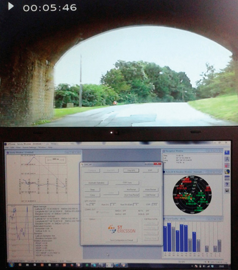
A small margin of recording bandwidth has been put to use with the ability to record video alongside the raw GNSS signals, and to replay it simultaneously. This allows developers not only to see the performance of their receiver in difficult signal environments, but also to gain a visual idea of the physical environment. Figure 12 shows a receiver control panel along with video pictures of the recorded environment.
Figure 12. GPS L1 and video synchronized replay
Conclusion
Early user feedback has validated the concept behind the device. Although the device will cover additional GNSS constellations and bands as they become operational, for the present the technology is stretched about as far as it can be consistent with the development of a timely and cost effective device. We will continue to address the compromises in the search for more performance, no doubt pushed by user demands.
Acknowledgment
The authors thank their colleagues at Integrated Navigation Systems and Spirent UK for support and access to design and user information.
Steve Hickling obtained his joint physics and electronics degree from the University of Birmingham. He is responsible for Spirent’s GNSS test solutions as lead product manager in the positioning business.
Tony Haddrell obtained his degree in physics at Imperial College, London, and is technical director at integrated Navigation Systems. He is a consultant to GNSS companies and a visiting lecturer at Nottingham University.
This article addresses how best to quantify “which navigation system performs best” in a realistic testing scenario. The methodology focuses on land vehicles navigating in urban environments, but applies equally well to pedestrian navigation and can be adapted for testing assisted-GNSS implementations. During a drive test, the truth-reference system and RF recording system log samples to disk, with no need for the receivers under test to be included during the actual drive.
By Eric Vinande, Brian Weinstein, Tianxing Chu, and Dennis Akos, University of Colorado, Boulder
FIGURE 1. Traditional in-vehicle receiver testing.
Radio frequency record-and-playback systems (RPS) have recently become commercially available. These systems sample the RF environment and store it to disk during a drive test and can replay it through receivers back in the lab environment. Here we explore the improvements in dynamic testing methodology created by these units.
RPS test system installation.
RPS constitute a stark contrast to more traditional signal simulators that use pre-defined trajectories and mathematical models to determine appropriate RF output. Signal simulators attempt to reproduce environmental error factors such as multipath, inertial aiding system errors, and building and vehicle obstructions. They rely on mathematical models to simulate these various error sources. In some cases they do a reasonable job of reproducing these errors, but the dynamic urban environment is so complex (for example, rapidly varying/fading signal strength(s), multiple multipath signals, short/long duration obstructions of multiple layers) that even a sophisticated mathematical model can not replicate all effects completely. Some simulators include software that enables the user to define a trajectory and a limited amount of urban scenario details. Again, only so much realism can be created in a simulation environment. Existing testing standards are simulator-based, and as such, are circumscribed by the signal simulator limitations in representing a dynamic environment.
Positioning performance of a satellite navigation receiver under test (RUT) is coupled with its RF front-end system and local oscillator quality. Because of the variation in RF components between RUTs, some likely have superior RF interference (RFI) immunity. RFI can be a serious issue in certain land vehicles due to on-board electrical systems or because of external interference sources.
This article describes a testing method applicable to all receiver types, and complementary to that described in the December 2009 GPS World article by Mitelman and colleagues, “Testing Software Receivers,” regarding validation testing within a production environment. Added elements include taking into account truth-system uncertainty and a repeatability verification of the RF playback process through non-deterministic hardware receivers.
We present here the dynamic testing approach currently used at the University of Colorado in Boulder for receiver evaluation and comparison in the urban environment. The approach also includes the ability to assess the effect of sensor augmentations (for example, inertial, environmental) on positioning performance.
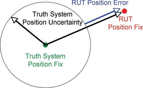
Truth Reference. Comparison with a truth reference system is essential for evaluation of satellite navigation receivers. For dynamic testing, this typically includes a survey-grade receiver coupled with a tactical-grade (or better) inertial measurement unit (IMU) and associated carrier-phase differential post-processing software. This software is filter-based and provides a positioning-error estimate in various components. Truth reference systems provide a continuous position estimate whose quality can vary depending on factors experienced in the urban environment, including length of full/partial satellite signal outage. In this study, we subtracted the 99th-percentile horizontal positioning error estimate of the truth system from the nominal RUT positioning error at each reporting epoch, as shown in Figure 2.
If the RUT position happens to lie within the truth-system position uncertainty, it is not considered to have any position error.
We focus here on a method to evaluate and compare mass-market, consumer-grade receivers to survey-grade receivers. One difference between these two receiver types is the way they handle the trade-off between accuracy and availability. Consumer receivers strive to provide the user with the highest availability, whereas survey receivers’ goal is to maximize accuracy. As a result, consumer-grade receivers will produce more regular position updates in harsh signal-tracking conditions, but must sacrifice accuracy to do so.
FIGURE 2. RUT position error calculation
Current Testing Standards
Currently accepted A-GPS standards such as those used by the 3rd Generation Partnership Project (3GPP) provide very limited dynamic testing in simulated urban conditions, being mainly designed to evaluate the first position calculation achieved in a particular simulated scenario. High-sensitivity receivers that pass or greatly exceed the 3GPP tests, in our opinion, are not guaranteed to have superior navigation performance in urban areas. Also, local oscillator performance is not specified. The trajectory dynamics imposed can actually be much smaller than the clock dynamics of a very low-cost local oscillator. A GPS receiver cannot tell the difference between the two and must track the effective Doppler variation.
The 3GPP defines five independent tests for A-GPS receiver certification. They include tests in the areas of: sensitivity with coarse/fine time assistance, nominal accuracy, dynamic range, multipath performance, and moving scenario/periodic update performance. The last three tests include elements that ostensibly pertain to the urban environment. These tests specify discrete, constant signal power levels for implementation in a hardware signal simulator. The discrepancy between the 3GPP-prescribed signal levels and those observed during actual drive testing is detailed as follows.
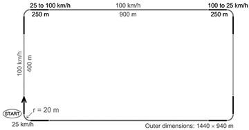
The 3GPP moving scenario/periodic update performance test trajectory is shown in Figure 3.
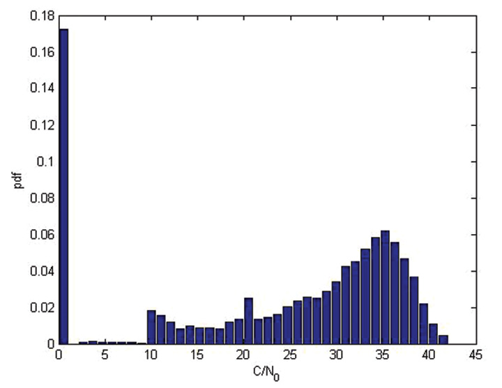
This test profile calls for the simulation of five satellites with a constant signal strength of 2130 dBm while the vehicle travels around the racetrack trajectory. In contrast, during an actual drive test in an urban area, a receiver reported the distribution of carrier-to-noise-density values for all tracked satellites as shown in Figure 4. This more accurately shows the range of signal strengths that should be expected in urban conditions.
FIGURE 4. Drive-test C/N0 distribution
The 3GPP moving test is considered passed if positions are reported regularly, and 95 percent of them are within 100 meters of the true position. This is not a particularly difficult test for a RUT to retain signal lock through, as the linear acceleration is about 0.15 g and the centripetal acceleration is about 0.25 g.
It is difficult for independent third parties to carry out a receiver evaluation following 3GPP guidelines as several of the tests require receiver restarts, which in turn requires testing automation. Depending on the receiver-evaluation hardware availability, restart commands may not be available to to an independent evaluator.
3GPP receiver testing results are quoted as pass or fail over a large number of short evaluations. For the dynamic environment, the system performance over continuous time is required to make a proper comparison between evaluated receivers.
In general, evaluating the GPS engines embedded within cell phones or other devices is difficult. Most are not made to interface with an external antenna, and the mere act of adding an antenna connection can significantly alter performance. The output format is not always documented, if it is even available to an end user. To allow fair across-the-board comparisons, GPS chipset manufacturers should make available development kits that have external antenna connections and well-documented message output formats.
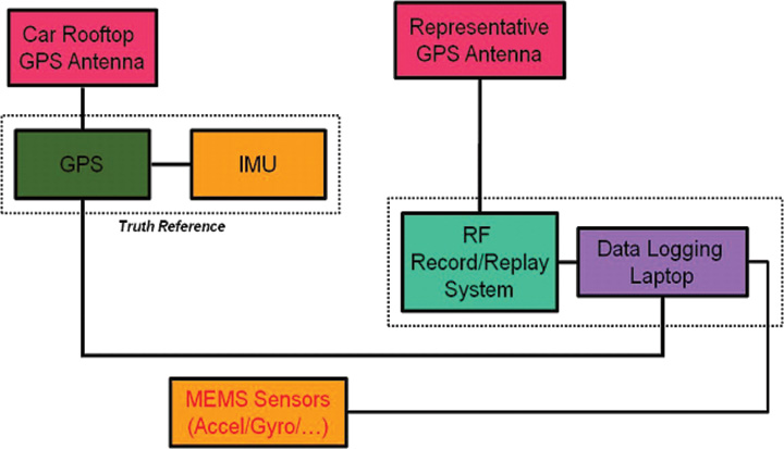
Drive-Test Configuration
Current live dynamic testing requires multiple systems to be operating in a moving vehicle (see opening Figure 1). A truth-reference system, usually a high-grade GPS/INS device along with post-processing, provides the basis to which all other RUT are compared. This system requires a dedicated vehicle rooftop antenna with the best possible sky view, separate from a lower-grade test antenna located within the vehicle. Each RUT is connected to the representative consumer-grade antenna located in the vehicle through a high-isolation splitter that suppresses inter-receiver interference. It is important at this point that the gain be set appropriately for each RUT, depending on the front-end expectations while maintaining an equivalent noise figure across all receivers.
Visualization Methods
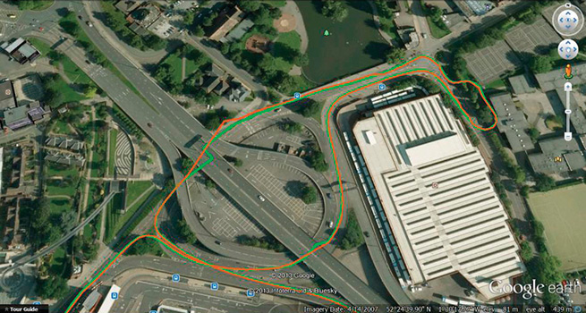
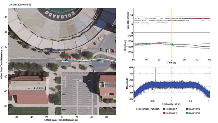
In addition to quantitative methods, we have created a qualitative visualization to assist with interpretation of the raw data. The same parsed data sets that provide the statistical script input are fed into a viewer script along with the post-processed truth reference data. With the truth-reference system data plotted in the center of the screen, each RUT is then plotted the correct distance and direction away, based on the distance and direction of error compared to truth. The receiver plots are overlaid onto Google Earth images centered on the truth-reference location. Plots of number of satellites utilized (top right of Figure 5) and elevation (middle right) as reported by each receiver and the sampled RF spectrum (lower right) are also included.
For each reporting epoch, based on the data frequency of the truth-reference system, a frame is generated with the aforementioned characteristics. These frames are gathered and encoded into a movie clip which can then be used as a quick and simple qualitative tool for receiver comparison. Figure 5 shows an individual movie frame. A forward-looking camera capability is also being added to this movie so the test environment can be documented from multiple angles.
FIGURE 5. Movie visualization screenshot
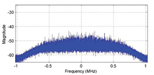
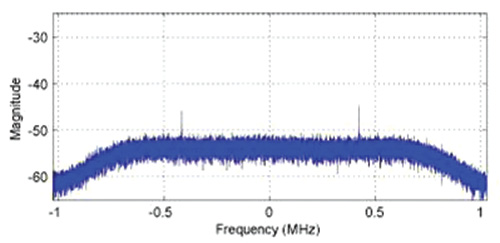
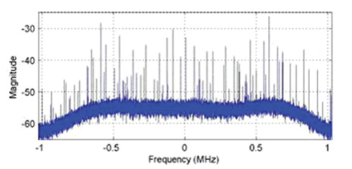
While observing this movie, variations in the sampled RF spectrum from interference or blockages can be associated with the current landscape. Locations of RFI sources can be identified and avoided (or included) in future testing. These RFI and significant blockage locations are of interest for receiver RF component and navigation filter development. The next three figures show spectrum snapshots during various parts of a drive test. In Figure 6, the cumulative GPS spectra rises above the noise floor and is visible during open sky conditions. While below ground level, Figure 7 shows only the front-end filter shape (and relatively minor RFI). Figure 8 shows an example of severe RFI when near a specific parking garage location.
FIGURE 6. Open-sky spectrum (centered on 1575.42 MHz)
FIGURE 7. Spectrum while below ground level (centered on 1575.42 MHz).
FIGURE 8. Spectrum near interference source (centered on 1575.42 MHz).
Record/Playback Concept
To overcome the limitations of hardware signal simulators and repeated vehicle drive testing, the RF record/playback testing method is utilized at the university. Commercially available equipment, capable of recording and playing back an RF signal, has recently become available. Equipment options exist for between $10,000–100,000, with 1–16 bit sampling and 4–25 MHz front-end bandwidth.
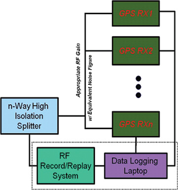
Figures 9 and 10 show the concept of “record once, playback many times.” During a drive test, the truth-reference system and RF recording system log samples to disk. There is no need for the RUT to be included during the actual drive test.
In the laboratory, the logged RF samples are replayed through a splitter to all RUT. The effect of receiver configuration changes can be evaluated without having to repeat the drive test. At a later time, additional receivers can also be tested using the same stored RF sample file.
During separate record and playback phases, testing considerations and methods discussed previously are implemented.
Since the recording process can only obviously capture current conditions, additional drive-test collections are required if different satellite geometry is desired, or if additional representative antennas need to be evaluated.
Repeatability of RPS Testing
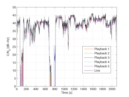
To validate that the playback signal levels were not significantly different from live signals, we conducted an urban, dynamic evaluation. Figure 11 shows that there is typically not more than a 1 dB difference in reported C/N0 between live and playback modes when testing a receiver that only reported integer values. The two dropout instances were excursions into parking garages.
FIGURE 11. Live and playback C/N0 values
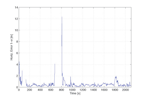
Figure 12 compares the navigation statistics between replays, using the same five playbacks as in Figure 11. The playbacks show a 1-sigma horizontal position solution spread under 1 meter for approximately 83 percent of the test.
FIGURE 12. Playback Horizontal Position Error Spread.
These two figures verify the repeatability of the RPS testing method and solidify it as an alternative to both signal-simulator testing and live testing of satellite navigation receivers.
Denver Testing Method
To evaluate the RPS concept, we conducted tests in three locations: Boulder, Denver, and Interstate Highway 70, all in Colorado. The Boulder and Denver locations were urban collections, while the Interstate 70 location was a natural canyon with significant elevation change. The collection at each location was repeated with two different representative antennas (patch and cell phone) at nearly the same sidereal time in order to keep the overhead satellite constellation similar.
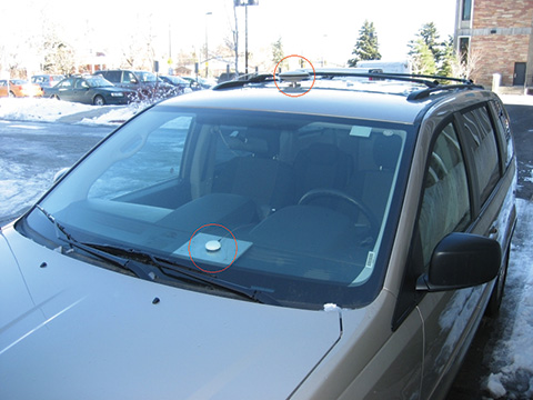
We examine here the November 11 and 16 Denver tests. The November 11 test used a patch antenna that places nearly all its gain in the upward direction, making it more immune to interfering sources below and to its sides. Figure 13 shows the patch antenn
a location on the van, as well as the truth-system antenna location utilized for testing on both days.
FIGURE 13. Patch antenna (dashboard) and truth-system antenna (rooftop) locations.
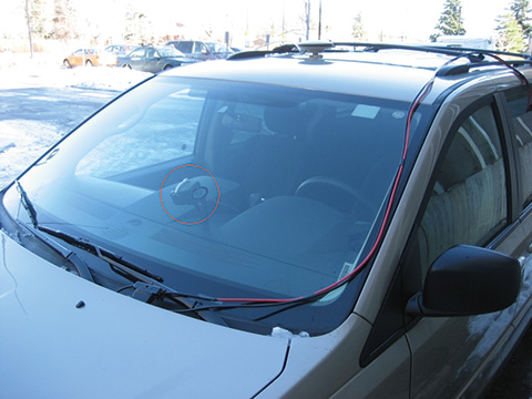
The November 16 test used a cell-phone GPS antenna that does not have a preferential gain direction, making it more susceptible to interfering sources below and to its sides. This antenna type is representative of the typical low-cost antenna (in some cases as simple as a piece of wire) found in consumer cell phones. Figure 14 shows the cell-phone antenna suction-cup mounted to the front window of the testing van. The representative antenna mounting location was chosen to minimize locally-generated RFI effects while also being representative of a typical vehicle-use case.
FIGURE 14. Cell-phone antenna location.
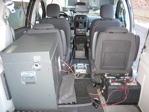
The required equipment and connections are minimal when performing RPS drive testing, as no RUTs are included. The inset to Figure 1 at the beginning of this article shows the RPS unit in the rear of the van, mounted on layers of foam to reduce vibration, which, if not properly addressed, can cause errors in mechanical hard drives writing data at high rates. Also visible are the truth receiver on the center of the van floor, and the car batteries for powering it and the IMU. The IMU is mounted to the vehicle frame and is not shown.
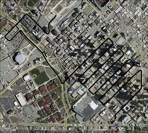
The test drive trajectory through Denver on November 11 and 16 as reported by the truth system is shown in black in Figure 15 and is also repeated in Figures 16 and 17. The test lasted approximately 40 minutes on both days. It started in the upper left part of Figure 15 and continued zig-zagging through downtown to the lower right.
FIGURE 15. Truth trajectory for November 11 and 16 tests.
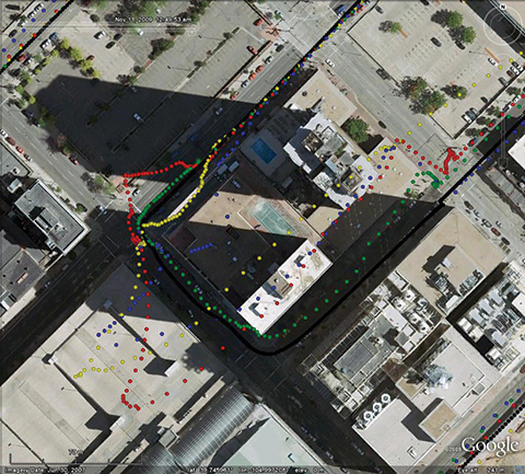
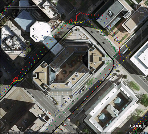
Figures 16 and 17 show particularly difficult blocks for the four receivers tested under the replay method. These receivers are denoted A (green), B (blue), C (red), and D (yellow).
FIGURE 16. Difficult block #1 during November 11 test and truth system antenna (rooftop) locations.
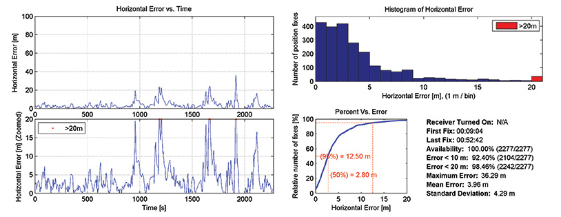
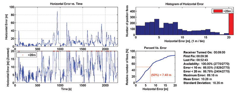
The horizontal positioning error statistics for two receivers on the November 11 test are shown in Figures 18 and 19. The left side shows horizontal error in two different zoom levels. The right side shows a histogram and cumulative distribution of errors, and several reporting metrics over the entire test. Even though receiver A in general outperformed receiver B, from the error time histories there are noticeable periods where both receivers simultaneously had positioning difficulties.
FIGURE 17. Difficult block #2 during November 11 test.
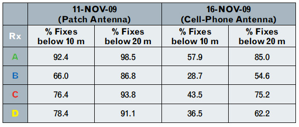
Table 1 summarizes the horizontal positioning statistics for all receivers during both tests. Positioning accuracy was severely degraded when replaying samples collected with the cell-phone antenna as compared to the patch antenna. Receiver A was the most accurate across both tests, while receiver B was the least accurate. The uncertainty of the truth system was subtracted out when producing the horizontal positioning results for all receivers.
Table 1
Conclusions
The record-and-playback system testing approach, in our opinion, represents the best way to test hardware receivers. It overcomes the fidelity limits of simulator-based testing, especially when considering the difficult-to-model urban environment. During receiver development, it requires only a single drive test for each location, as sampled RF data can be replayed from disk.
Having demonstrated that RPS testing is repeatable, we have produced a library of RF sample files representing real-world conditions for continued receiver development and testing purposes.
Eric Vinande is Ph.D. student at the University of Colorado studying GPS/MEMS inertial sensor integration and urban RFI aspects.
Brian Weinstein is a BSEE student participating in the Undergraduate Research Opportunity Program for GNSS receiver testing at the University of Colorado.
Tianxing Chu is a visiting researcher at the University of Colorado from Peking University where he is a Ph.D. student.
Dennis Akos is an associate professor within the Aerospace Engineering Sciences Department at the University of Colorado with concurrent appointments at Stanford University and Luleå University of Technology.
Manufacturers
Development of the methodology described here used two different RPS systems, one from LabSat (RaceLogic) and one from Averna. The test data come from the Averna system.