Tag: Ring of Fire

  • Research Roundup: Atmospheric effects on GNSS

    Research Roundup: Atmospheric effects on GNSS

    Photo: buradaki/iStock/Getty Images Plus/Getty Images
    Photo: buradaki/iStock/Getty Images Plus/Getty Images

    GNSS researchers presented hundreds of papers at the 2022 Institute of Navigation (ION) GNSS+ conference, which took place Sept. 19–23 in Denver, Colorado, and virtually. The following five papers focused on atmospheric effects on GNSS signals. The papers are available at www.ion.org/publications/browse.cfm. 

    Addressing Scintillation Error

    Mitigating the scintillation effect at low latitude is a complex matter: several kinds of experimental data must be collected, realistic models must be developed, and, most importantly, useful real-time indices and alerts must be made available.

    The authors introduce a prototype based on a patent owned by SpacEarth Technology to address scintillation error detection and mitigation, supporting precision GNSS-based services at low latitudes in any season and space weather conditions. The patent relates to a method of total electron content (TEC) and scintillation empirical forecasting, in particular short-term forecasting (seconds to minutes). The output of the method is necessary to feed mitigation algorithms aiming at improving accuracy on GNSS precise positioning techniques (RTK, NRTK, and PPP) under ionospheric harsh conditions.

    The prototype is designed with a Central Elaborating Facility, which collects the data provided by a network of GNSS monitoring stations detecting scintillation events, and broadcasts foreseen scintillation parameters. Users with a rover mitigation device can apply the parameters from the central facility for scintillation error mitigation. 

    Vincenzo Romano, INGV and SpacEarth Technology; Claudio Cesaroni, INGV; Luca Spogli, Alessandro Fiorini, INGV and SpacEarth Technology; Marco Fermi, Gter; Lorenzo Benvenuto, Gter and University of Genoa; Tiziano Cosso, Gter; Marcin Grzesiak, SRC/PAS; Joao Francisco Galera Monico, Italo Tsuchiya, UNESP; Gabriel Oliveira, Marcos Guandalini; “Ionospheric Scintillation Mitigation at Low Latitude to Improve Navigation Quality.”

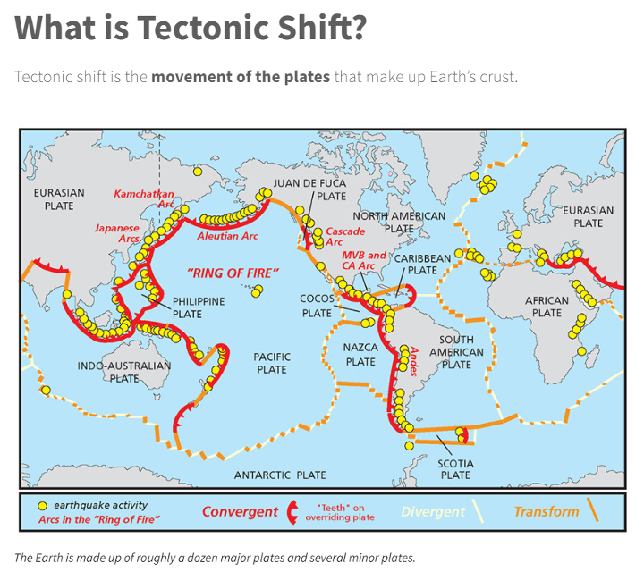
    Ring of Fire GUARDIAN 

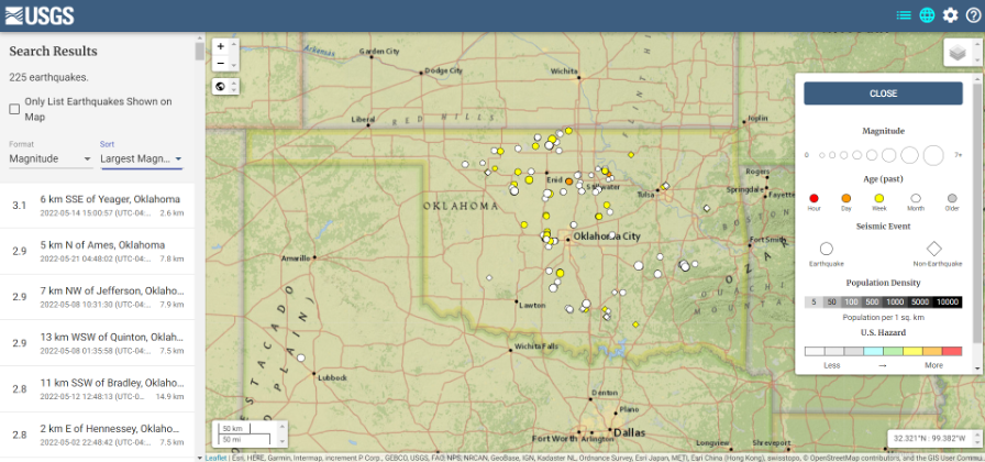
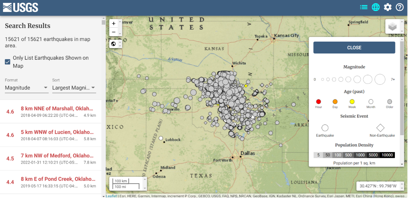
    Commonly, natural hazards release energy into the Earth’s atmosphere in the form of acoustic-gravity waves, which propagate up to the ionosphere. The resulting traveling ionospheric disturbances (TIDs) can be detected using GNSS signals, through the computation of the integrated total electron content (TEC) along the lines of sight between GNSS receivers and satellites. The global distribution of ground-based GNSS receivers constantly tracking multiple GNSS constellations (GPS, Galileo, GLONASS, BeiDou, and others) provides excellent spatio-temporal coverage around the world, including in areas of limited coverage by existing warning systems.

    The authors present the operational GNSS-based Upper Atmospheric Real-time Disaster Information and Alert Network (GUARDIAN). Based on dual-frequency GNSS data from the Global Differential GPS (GDGPS) network of the Jet Propulsion Laboratory, the GUARDIAN architecture computes slant TEC time series in near real time.

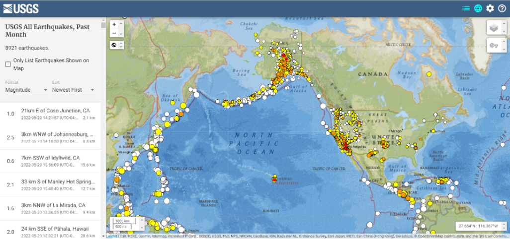
    As part of the GDGPS network, 78 stations around the Pacific ring of fire monitor the four GNSS constellations: GPS, Galileo, GLONASS and BeiDou. Cycle slips are corrected and the time series are filtered, both in real time. The resulting data stream is output live to a user-friendly public website, benefitting the general public and the scientific community. 

    The current GUARDIAN focuses on the Pacific region. However, the architecture can readily be extended to a worldwide coverage.

    Léo Martire, S. Krishnamoorthy, L. J. Romans, B. Szilágyi, P. Vergados, A. W. Moore, A. Komjáthy, Y. E. Bar-Sever, A. B. Craddock, NASA Jet Propulsion Laboratory, California Institute of Technology; “GUARDIAN: A Near Real-Time Ionospheric Monitoring System for Natural Hazards Early Warnings.”

    Civil Aviation Interference

    The authors provide a survey on GNSS receiver architectures with emphasis on new carrier-tracking techniques for mitigating the adverse effect of ionospheric scintillation within the context of civil aviation. The survey is complemented by results gathered from simulations on the impact of ionospheric scintillation in conventional receiver architectures. A review on scintillation mitigation techniques is carried out, covering several “technique families,” highlighting their potential for performance improvement, as well as their shortcomings and challenges in implementation.

    A semi-analytical simulation campaign is carried out for different modulations: L1, L5 for GPS, and E1, E5a for Galileo. Here, the performance of a standard receiver tracking a set of GPS and Galileo satellites affected by ionospheric scintillation is analyzed to pinpoint existing vulnerabilities to this effect.

    The simulation results show that ionospheric scintillations are responsible for large variations in carrier-to-noise ratio, which in turn can be responsible for losses of lock and large phase variations, increasing phase RMSE and in some cases leading to cycle slips of the phase estimation. Thus, the adopted solution must be robust to signal power fluctuations and the occurrence of cycle slips and able to maintain phase lock.

    António Negrinho, GMV-PT Pedro Boto, GMV-PT Marta Cueto, GMV-ES Mikael Mabilleau, EUSPA Claudia Paparini, EUSPA Ettore Canestri, EUSPA; “Survey on Signal Processing Techniques for GNSS Ionospheric Scintillation Mitigation.”

    Tonga Eruption Data Analyzed

    Extreme natural disasters, such as volcanic eruptions, can create visible pressure waves in the atmosphere and trigger observable ionospheric wave responses that can travel hundreds of kilometers in the ionosphere. The acoustic and gravity waves generated can cause ionospheric TEC perturbations and variations. The TEC determines the GNSS ionospheric delay and can cause significant positioning errors, which may affect the performance of GNSS-based applications.

    The researchers processed GNSS data collected from the Hong Kong Satellite Positioning Reference Station Network to analyze the ionospheric activity and positioning performance responding to the Tonga volcanic eruption on Jan. 15, 2022. To detect and repair cycle-slip jumps, the researchers applied theTEC rate and Melbourne Wubbena Wide Lane (MWWL) linear combinations. A Savitzky-Golay low-pass filter with a 30s window was used to improve the TEC accuracy.

    The team investigated the changes in TEC, Rate of TEC index (ROTI) and positioning errors in the eastward, northward and upward directions after the anomalous ionospheric propagation to Hong Kong between 11:30 and 14:30. The team found the ionospheric anomaly could generate large changes in the three parameters, with peaks up to three times the calm period. Their prompt research contributes to a better understanding of the coupling of extreme ionospheric activities and dynamics caused by volcanic eruptions. 

    Xiaojia Chang, Kai Guo, Zhipeng Wang, Kun Fang, Hongxia Wang, Beihang University; Hailong Chen, China Academy of Aerospace Electronics Technology; “Ionospheric Anomaly and GNSS Positioning Responses to the January 2022 Tonga Volcanic Eruption.” 

    Toolbox for Monitor Network

    The MONITORtoolbox is a set of Python-coded software tools to perform automatized large-scale processing of data from the Monitor network of the European Space Agency (ESA). The Monitor network aims to continuously monitor ionospheric scintillation events from multiple ground stations strategically located around the globe. It accommodates a repository with a large number of GNSS measurements containing scintillation events for users to analyze scintillation data or for research purposes.

    This paper shows the potential of the MONITORtoolbox for providing access to a large amount of data that otherwise, without a systematic processing, becomes practically useless. The software developed implements the means to collect data and store it in a local database for quick offline access. It detects the presence of scintillation events based on certain conditions and criteria defined by the user and identifies its properties in terms of duration, time of occurrence, intensity and satellite location. It implements the tools to compute relevant statistics, providing insights on ionospheric scintillation phenomena.

    Sergi Locubiche-Serra, Alejandro Pérez-Conesa, Diego Fraile-Parra, Gonzalo Seco-Granados, José A. López-Salcedo, Universitat Autònoma de Barcelona, IEEC-CERES; Juan M. Parro-Jiménez, Raúl Orús-Pérez, ESTEC, European Space Agency; “MONITORtoolbox — Software Tool for the Analysis of Ionospheric Scintillation Data from the ESA Monitor Network.” 
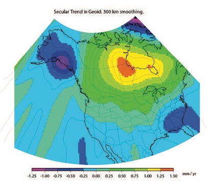
  • The effects of geoid changes in NGS’s new, modernized 2022 NSRS

    The effects of geoid changes in NGS’s new, modernized 2022 NSRS

    My April column addressed the vertical movement at the NOAA CORS Network (NCN). The values at the sites indicate the potential movement of marks in the area of the CORS. The rates are based on GNSS data and have an estimate of error associated with them.

    As I mentioned in my previous column, I’m not sure how the National Geodetic Survey (NGS) will address the vertical movement effects in the new, modernized National Spatial Reference System (NSRS). That said, NGS will be monitoring the CORS and looking for trends to help describe the vertical movement at the CORS. These trends are an indication of what may be happening in that area.

    As stated in previous columns, orthometric heights in NAPGD2022 will be defined through ellipsoid heights and a geoid model, for example GEOID2022. In addition to the movement of individual marks due to crustal movement, there are geophysical reasons for changes in the geoid that affect the orthometric height of a mark. Therefore, changes in the geoid model will be very important to users estimating orthometric heights using GNSS.

    As stated in the NOS NGS 64 report, NGS has set a goal of maintaining geoid accuracy at 1 centimeter (1 standard deviation) in both absolute and differential geoid undulations. The box titled “Figure 13 from NOS NGS 64 Report” depicts an estimate of the secular change in the geoid. As indicated in the plot, the changes are very small, ranging from -1.25 mm/year to 1.5 mm/year.

    What I find interesting is the small negative change in the southeastern United States. There are other drivers for geoid changes. This column will address some of these changes and what they mean to users.

    Secular geoid change

    Photo: NGS
    Figure 13 from NOS NGS 64 Report (Image: NGS)

    As mentioned in many of my articles, the new, modernized NSRS has a time-dependent component. This includes the geoid modelTable 5-1 from NOS NGS 64 report are examples of some of the physical processes being investigated by NGS to account for changes in the geoid.  (See the box titled “Some of the geophysical drivers of geoid change.”) As mentioned in the NOS NGS 64 report, the magnitudes in red have already been determined to be too small for NGS to model. The examples highlighted in yellow have magnitudes that are significant and NGS will attempt to account for these changes to the geoid. 

    Table 5-1: Some of the geophysical drivers of geoid change
    Table 5-1: Some of the geophysical drivers of geoid change

    NGS classifies the changes in the geoid in three different groups: Shape Change, Size Change, and W0 Change. The box titled “The Groups of Geoid Change” provides NGS’s definition and explanation of the terms.

    The groups of geoid change

    Photo: Dave Zilkoski

    NGS’s report on their Geoid Monitoring Service (GeMS) program provides figures that depict an estimate of the secular geoid rate trend based on the NASA GSFC mascon model. See the boxes titled “Estimate of Geoid Rate Over CONUS” and “Estimate of Geoid Rate Over Alaska.” For more details on GeMS, download the report NOAA Technical Report NOS NGS 69: A Preliminary Investigation of the NGS’s Geoid Monitoring Service (GeMS), and read my December 2019 Survey Scene column. The secular geoid rate trend is an example of the geoid changing its shape, but not the W0 value. What this means is that the local geoid undulations will change, but the overall size of the geoid will not.

    Estimate of geoid rate over CONUS

    Figure 32: Geoid rate over CONUS based on the GSFC mascon model [mm/yr] (Image: NOAA)
    Figure 32: Geoid rate over CONUS based on the GSFC mascon model [mm/yr] (Image: NOAA)
    Estimate of geoid rate over Alaska

    Figure 33: Geoid rate over Alaska from GSFC mascon model [mm/yr] (Image: NOAA)
    Figure 33: Geoid rate over Alaska from GSFC mascon model [mm/yr] (Image: NOAA)
    These changes in the geoid are fairly small values (+/- 1.3 mm/year), but they will accumulate over a decade. As previously stated, NGS’s goal is to maintain geoid accuracy at the centimeter level (1 standard deviation) in both absolute and differential geoid undulations. In my February 2022 column, I discussed how coordinates change because Earth’s surface is moving due to the movement of major tectonic plates. It’s fairly obvious how the tectonic shift affects horizontal coordinates, but earthquakes and volcanic eruptions can also cause large shifts in vertical coordinates.

    In recent history, on May 18, 1980, geologists watched in awe as Mount St. Helens erupted in a gigantic explosion. After the eruption, the volcanic cone of Mount St. Helens had been completely blasted away; the peak, which was at an elevation of 9,677 feet (2,950meters) was changed to a horseshoe-shaped crater with an elevation of 8,363 feet (2,549 meters). Extreme crustal movements such as the Mount St. Helens eruption can change the shape of the geoid. As explained in my April 2022 newsletter, NGS understands this and is attempting to manage the changing coordinates by providing a time-dependent component to a mark’s ellipsoid height, but there is also a time-dependent component to the geoid that affects the mark’s orthometric height.

    Ring of Fire

    Image: National Ocean Service
    Image: National Ocean Service

    The “Ring of Fire” map highlights earthquake activities around the world. As indicated in Table 5.1, earthquake or volcanic eruptions can change the shape of the geoid. Of course, they also can change the height of a mark due to crustal movement, which would typically be larger than the change in the geoid height. The amount of movement would be due to the size and magnitude of the event, but even small earthquakes could cause a change in the height of a mark located near the event. Earthquakes are occurring all over the world every day. 

    Earthquakes with large magnitudes are highlighted by news media outlets, but ones with smaller magnitude typically are not highlighted. The four figures below provide examples of earthquakes that have occurred over 30 days. This information can be obtained from the United States Geological Survey (USGS).

    Earthquakes during the past 30 Days
    Date: May 20, 2022

    Image: USGS
    Image: USGS

    Earthquakes in the lower 48 during the past 30 days
    Date: May 20, 2022

    Image: USGS
    Image: USGS

    Earthquakes in eastern United States in the past 30 days
    Date: May 20, 2022

    Image: USGS
    Image: USGS

    I found the large number of earthquakes that occurred in Oklahoma in just 30 days to be very interesting.  This isn’t something that I thought occurred in the eastern region of the United States. 

    Earthquakes in Oklahoma during the past 30 days
    Date: May 20, 2022

    Image: USGS
    Image: USGS

    The image below depicts earthquakes that have occurred in Oklahoma in the past five years. They are fairly small in magnitude, but what is the cumulative effect on the geoid in the region, as well as changes to the orthometric heights of marks due to crustal moment in the region?  This is why it is important for the new, modernized NSRS to implement time-dependent coordinates. 

    Earthquakes in Oklahoma in the last 5 years
    Dates: 2017 to 2022

    Image: USGS
    Image: USGS

    To better understand the changes to the geoid, NGS performed a survey in Alaska to obtain geodetic data as part of its GeMS program.  On May 12, 2022, Kevin Ahlgren, a geodesist at NGS, described in a webinar the observations collected and some of the results. 

    The presentation provided an overview of a field campaign performed in support of the GeMS program and a time-dependent geoid model. The campaign included static GNSS, relative gravity, and deflection of the vertical techniques on 50 stations in Alaska. The webinar was can be downloaded.

    I encourage everyone to download the presentation.  The change in the geoid due to geophysical drivers is small, but if the new, modernized NSRS is going to include time-dependent coordinates, then changes in the geoid must be accounted for.  For demonstration purposes, NGS provides an example of the time-dependent geoid change in the xGEOID20 webtool.  The box below, “xGEOID20 interactive computation output,” is an example of using this tool. The two stations are located in Alaska. As indicated in the output from the tool, the change in the geoid is 8 mm in five years. Again, NGS’s goal is to maintain geoid accuracy at the centimeter level (1 standard deviation) in both absolute and differential geoid undulations.  These small changes can become significant over time. 

    xGEOID20 interactive computation output

    Note: DN is the time-dependent geoid change computed between user inputted epoch (t) and t.
    Note: DN is the time-dependent geoid change computed between user inputted epoch (t) and t. (Image: NGS)

    The last geoid change group that I’ll highlight has to do with the change in the gravity potential (W0) value that defines the model. The NOS NGS 64 Report states that the standing definition of the geoid, as adopted and used at NGS, is the following:  

    The geoid is the equipotential surface of the Earth’s gravity field which best fits, in a least squares sense, global mean sea level. 

    As stated in the NOS NGS 64 report, over a century of sea-level measurements imply that global mean sea level (GMSL) was rising at a rate of approximately 1.7 millimeters per year and was rising at a rate of 3.2 millimeters per year between 1993 and 2010 (IPCC, 2014). If NGS is going to define the geoid as the equipotential surface of the Earth’s gravity field that best fits, in a least squares sense, global mean sea level, then the geoid in the new, modernized NSRS must change when the GMSL exceeds a certain threshold. 

    Again, NGS’ goal is to maintain geoid accuracy at the centimeter level (1 standard deviation) in both absolute and differential geoid undulations.  What this means is that as GMSL rises, the value of gravity potential which best fits to GMSL (called W0) will also change.  In other words, the surface which was called “the geoid” and had W=W0 in 2022 will no longer be the geoid. A new value of W0 (W0new) is chosen, and “the geoid” would now be the surface W=W0new.   

    So, what does this really mean to users? The NOS NGS 64 Report states on page 37:

    “NGS and the Canadian Geodetic Survey have jointly adopted the value of 2.0 m^2/s^2 as the replacement threshold for a new geoid model (and new geopotential datum). This represents approximately 20 centimeters of GMSL (and thus geoid) rise. At the current rate of sea-level change of about +3 millimeters per year (IPCC, 2014), this means NGS expects to replace NAPGD2022 in approximately 60 to 70 years.” 

    Therefore, this should not be a major concern of users for a long time. 

    This column highlighted that orthometric heights in NAPGD2022 will be defined through ellipsoid heights and a geoid model, for instance GEOID2022; and therefore, changes in the geoid model will be very important to users estimating orthometric heights using GNSS.  It briefly described the geophysical reasons for changes in the geoid that affect the orthometric height of a mark. 

    If NGS is going to meet the goal of maintaining geoid accuracy at 1 centimeter (1 standard deviation) in both absolute and differential geoid undulations, they will have to address changes in the geoid. The secular changes in the geoid, as indicated in Figure 13 in the NOS NGS 64 report, are very small, ranging from -1.25 mm/year to 1.5 mm/year. Once again, these are small changes to the geoid, but they will accumulate over time, and that is why NGS is including time-dependent coordinates in the new, modernized NSRS.