Tag: risk assessment

  • Make it real: Developing a test framework for PNT systems and devices

    Make it real: Developing a test framework for PNT systems and devices

    Tests of the robustness of commercial GNSS devices against threats show that different receivers behave differently in the presence of the same threat vectors. A risk-assessment framework for PNT systems can gauge real-world threat vectors, then the most appropriate and cost-effective mitigation can be selected.

    Vulnerabilities of GNSS positioning, navigation and timing are a consequence of the signals’ very low received power. These vulnerabilities include RF interference, atmospheric effects, jamming and spoofing. All cases should be tested for all GNSS equipment, not solely those whose applications or cargoes might draw criminal or terrorist attention, because jamming or spoofing directed at another target can still affect any receiver in the vicinity.

    GNSS Jamming. Potential severe disruptions can be encountered by critical infrastructure in many scenarios, highlighting the need to understand the behavior of multiple systems that rely on positioning, and/or timing aspects of GNSS systems, when subject to real-world GNSS threat vectors.

    GNSS Spoofing. This can no longer be regarded as difficult to conduct or requiring a high degree of expertise and GNSS knowledge. In 2015, two engineers with no expertise in GNSS found it easy to construct a low-cost signal emulator using commercial off-the-shelf software–defined radio and RF transmission equipment, successfully spoofing a car’s built-in GPS receiver, two well-known brands of smartphone and a drone so that it would fly in a restricted area.

    In December 2015 the Department of Homeland Security revealed that drug traffickers have been attempting to spoof (as well as jam) border drones. This demonstrates that GNSS spoofing is now accessible enough that it should begin to be considered seriously as a valid attack vector in any GNSS vulnerability risk assessment.

    More recently, the release of the Pokémon Go game triggered a rapid development of spoofing techniques. This has led to spoofing at the application layer: jailbreaking the smartphone and installing an application designed to feed faked location information to other applications. It has also led to the use of spoofers at the RF level (record and playback or “meaconing”) and even the use of a programmed SDR to generate replica GPS signals — and all of this was accomplished in a matter of weeks.

    GNSS Segment Errors. Whilst not common, GNSS segment errors can create severe problems for users. Events affecting GLONASS during April 2014 are well known: corrupted ephemeris information was uploaded to the satellite vehicles and caused problems to many worldwide GLONASS users for almost 12 hours. Recently GPS was affected. On January 26, 2016, a glitch in the GPS ground software led to the wrong UTC correction value being broadcast. This bug started to cause problems when satellite SVN23 was withdrawn from service. A number of GPS satellites, while declaring themselves “healthy,” broadcast a wrong UTC correction parameter.

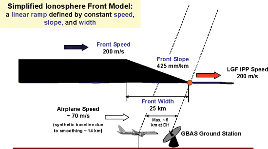
    Atmospheric Effects. Single frequency PNT systems generally compensate for the normal behavior of the ionosphere through the implementation of a model such as the Klobuchar Ionospheric Model.

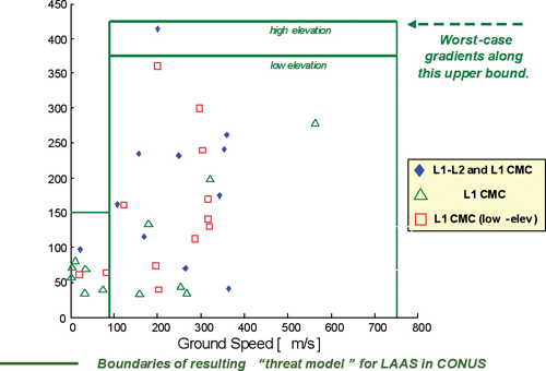
    Space weather disturbs the ionosphere to an extent where the model no longer works and large pseudorange errors, which can affect position and timing, are generated. This typically happens when a severe solar storm causes the Total Electron Count (TEC) to increase to significantly higher than normal levels.

    Dual-frequency GNSS receivers can provide much higher levels of mitigation against solar weather effects. However, this is not always the case; during scintillation events dual frequency diversity is more likely to only partially mitigate the effects of scintillation.

    Solar weather events occur on an 11-year cycle; the sun has just peaked at solar maximum, so we will find solar activity decreasing to a minimum during the next 5 years of the cycle. However that does not mean that the effects of solar weather on PNT systems should be ignored for the next few years where safety or critical infrastructure systems are involved.

    TEST FRAMEWORK

    Characterization of receiver performance, to specific segments within the real world, can save either development time and cost or prevent poor performance in real deployments. Figure 1 shows the concept of a robust PNT test framework that uses real-world threat vectors to test GNSS-dependent systems and devices.

    We have deployed detectors — some on a permanent basis, some temporary — and have collected extensive information on real-world RFI that affects GNSS receivers, systems and applications.

    For example, all of the detected interference waveforms in Figure 2 have potential to cause unexpected behavior of any receiver that was picking up the repeated signal. A spectrogram is included with the first detected waveform for reference as it is quite an unusual looking waveform, which is most likely to have originated from a badly tuned, cheap jammer. The events in the figure, captured at the same European sports event, are thought to have been caused by a GPS repeater or a deliberate jammer. A repeater could be being used to rebroadcast GPS signals inside an enclosure to allow testing of a GPS system located indoors where it does not have a view of the sky.

    The greatest problem with GPS repeaters is that the signal can “spill” outside of the test location and interfere with another receiver. This could cause the receiver to report the static position of the repeater, rather than its true position. The problem is how to reliably and repeatedly assess the resilience of GPS equipment to these kinds of interference waveforms. The key to this is the design of test cases, or scenarios, that are able to extract benchmark information from equipment. To complement the benchmarking test scenarios, it is also advisable to set up application specific scenarios to assess the likely impact of interference in specific environmental settings and use cases.

    TEST METHODOLOGY

    A benchmarking scenario was set up in the laboratory using a simulator to generate L1 GPS signals against some generic interference waveforms with the objective of developing a candidate benchmark scenario that could form part of a standard methodology for the assessment of receiver performance when subject to interference.

    Considering the requirements for a benchmark test, it was decided to implement a scenario where a GPS receiver tracking GPS L1 signals is moved slowly toward a fixed interference source as shown in Figure 3.

    The simulation is first run for 60 seconds with the “vehicle” static, and the receiver is cold started at the same time to let the receiver initialise properly. The static position is 1000m south of where the jammer will be. At t = 60s the “vehicle” starts driving due north at 5 m/s. At the same time a jamming source is turned on, located at 0.00 N 0.00 E. The “vehicle” drives straight through the jamming source, and then continues 1000m north of 0.00N 0.00E, for a total distance covered of 2000m. This method is used for all tests except the interference type comparison where there is no initialization period, the vehicle starts moving north as the receiver is turned on.

    The advantages of this simple and very repeatable scenario are that it shows how close a receiver could approach a fixed jammer without any ill effects, and measures the receiver’s recovery time after it has passed the interference source. We have anonymized the receivers used in the study, but they are representative user receivers that are in wide use today across a variety of applications. Isotropic antenna patterns were used for receivers and jammers in the test. The test system automatically models the power level changes as the vehicle moves relative to the jammer, based on a free-space path loss model.

    RESULTS

    Figure 4 shows a comparison of GPS receiver accuracy performance when subject to L1 CHIRP interference. This is representative of many PPD (personal protection device)-type jammers.
    Figure 5 shows the relative performance of Receiver A when subject to different jammer types — in this case AM, coherent CW and swept CW.

    Finally in Figure 6 the accuracy performance of Receiver A is tested to examine the change that a 10dB increase in signal power could make to the behavior of the receiver against jamming — a swept CW signal was used in this instance.

    Discussion. In the first set of results (the comparison of receivers against L1 CHIRP interference), it is interesting to note that all receivers tested lost lock at a very similar distance away from this particular interference source but all exhibited different recovery performance.

    The second test focused on the performance of Receiver A against various types of jammers — the aim of this experiment was to determine how much the receiver response against interference could be expected to vary with jammer type. It can be seen that for Receiver A there were marked differences in response to jammer type. Finally, the third test concentrated on determining how much a 10dB alteration in jammer power might change receiver responses. Receiver A was used again and a swept CW signal was used as the interferer. It can be seen that the increase of 10dB in the signal power does have the noticeable effect one would expect to see on the receiver response in this scenario with this receiver.

    Having developed a benchmark test bed for the evaluation of GNSS interference on receiver behavior, there is a great deal of opportunity to conduct further experimental work to assess the behavior of GNSS receivers subject to interference. Examples of areas for further work include:

    • Evaluation of other performance metrics important for assessing resilience to interference
    • Automation of test scenarios used for benchmarking
    • Evaluation of the effectiveness of different mitigation approaches, including improved antenna performance, RAIM, multi-frequency, multi-constellation
    • Performance of systems that include GNSS plus augmentation systems such as intertial, SBAS, GBAS

    CONCLUSIONS

    A simple candidate benchmark test for assessing receiver accuracy when subjected to RF interference has been presented by the authors.

    Different receivers perform quite differently when subjected to the same GNSS + RFI test conditions. Understanding how a receiver performs, and how this performance affects the PNT system or application performance, is an important element in system design and should be considered as part of a GNSS robustness risk assessment.

    Other GNSS threats are also important to consider: solar weather, scintillation, spoofing and segment errors.

    One of the biggest advantages of the automated test bench set-up used here is that it allows a system or device response to be tested against a wide range of of real world GNSS threats in a matter of hours, whereas previously it could have taken many weeks or months (or not even been possible) to test against such a wide range of threats.

    Whilst there is (rightly) a lot of material in which the potential impacts of GNSS threat vectors are debated, it should also be remembered that there are many mitigation actions that can be taken today which enable protection against current and some predictable future scenarios.

    Carrying out risk assessments including testing against the latest real-world threat baseline is the first vital step towards improving the security of GNSS dependent systems and devices.

    ACKNOWLEDGMENTS

    The authors would like to thank all of the staff at Spirent Communications, Nottingham Scientific Ltd and Qascom who have contributed to this paper. In particular, thanks are due to Kimon Voutsis and Joshua Stubbs from Spirent’s Professional Services team for their expert contributions to the interference benchmark tests.

    MANUFACTURERS

    The benchmarking scenario described here was set up in the laboratory using a Spirent GSS6700 GNSS simulator.

  • Expert Advice: Integrity: Lessons from the 2008 Financial Collapse

    Sam Pullen
    Sam Pullen

    By Sam Pullen

    Deterministic risk modeling, the basis of the Efficient Market Hypothesis (EMH) at the core of modern quantitative finance, is known to be fundamentally flawed, but its elegance and convenience has blinded researchers to growing evidence of its weaknesses. The near-complete acceptance of the EMH led to models that dramatically accentuate its flaws, which in turn led to absurd but eagerly accepted conclusions for loan-default risk. These models proved dramatically vulnerable to changes in the housing market in 2007–2008 and led directly to the ensuing crash.

    The gross inattention to potential anomalies and violations of nominal behavior that characterize quantitative finance fortunately do not apply to satellite navigation integrity assurance. Similar techniques and probability distributions are used, but understanding what can go wrong leads to detailed emphasis on modeling and mitigating rare events. Where significant uncertainty exists, conservative assumptions try to be robust to it. Thus, certification of satellite- and ground-based augmentation systems (SBAS and GBAS) likely demonstrates that these systems meet their integrity risk requirements with substantial margin.

    Despite this, the predominant use of deterministic models for risk assessment is dangerous because it purports to provide guaranteed bounds on uncertainty that do not apply in practice. The conservative nature of satellite navigation risk assessment greatly reduces but cannot eliminate the underlying integrity risk, while it leads to performance losses with potentially unmeasured safety impacts. Given the uncertainty that is present, probabilistic models are much better suited to providing “illusion-free” risk assessments that enable realistic system-level design trade-offs.

    Economics. Decades of financial theory are based upon the assumption that the normal (Gaussian) distribution applies to financial markets. In spite of common-sense arguments to the contrary, assuming that it does is too convenient to give up, and the theories it gives rise to are so useful that it was thought better to force-fit the model to financial processes. Academic and professional preference for tractable, analytical, easy-to-use models trumped the search for truth.

    The simplification of correlation into a single parameter made it easier to fit historical data on mortgage default risk correlation to a tractable model. Despite this, the relative rarity of defaults prior to 2000 made any correlation model based on historical default data highly uncertain. An EMH-based market-driven model for default risk correlation became instantly popular, enabling the creation of complicated mortgage-backed derivatives without in-depth analysis.

    The simplicity of the Value-at-Risk output that encouraged its widespread use in corporte risk assessment allowed managers to forget that it was only useful to, at most, the 99th percentile. It quickly became thought of as an actual worst-case bound on losses and treated as such in portfolio optimization. Loss reserves throughout the economy fell far short of what was needed. In retrospect, such approaches that oversimplify risk to the point where managers think they fully understand it are worse than useless, as they are so likely to be abused. Experts should understand risk in all its complexity and communicate that risk to decision-makers as fully as possible.

    Mathematics. This financial experience suggests that, as Albert Einstein said, “As long as the laws of mathematics refer to reality, they are not certain; and as far as they are certain, they do not refer to reality.”

    Deterministic models provide precise quantification of uncertainty whose accuracy and precision are illusory because they depend wholly on the assumptions used to generate the results. Probabilistic models also produce imprecise outputs, but the imprecision is real, and the goal of these models is to identify this lack of precision, rather than cover it up.

    Because the probabilistic approach is so philosophically different from the deterministic one, it is likely that more traditional deterministic risk models will remain dominant. These require multiple assumptions regarding uncertain behavior and simplifications to make the resulting model tractable and useful for analysis. Danger lies in forgetting how these models were created and growing to believe in them too strongly while ignoring all contrary data, as happened with the EMH.

    To avoid this, assumptions and simplifications on which deterministic risk models are based should be highlighted not only during the modeling process but also when results are presented. If these shaky foundations are consistently emphasized, fewer people will be tempted to willfully or accidentally misinterpret the results, and researchers will be less likely to extrapolate from one flawed model to another.

    Lessons for SatNav Integrity

    We must first recognize that integrity or safety assurance for satellite navigation is a unique application of risk assessment in which the aim is to protect passengers from the consequences of very rare but potentially hazardous threats. As in the financial world, the Gaussian probability distribution is used extensively to model nominal error behavior and to compute position-domain protection levels intended to bound worst-case user position errors at the integrity-risk probabilities required for user safety. The Gaussian model is a convenient, efficient means to communicate ground-system errors to SBAS and GBAS users in a single parameter: the standard deviation (or sigma) of range-domain errors.

    Great care is taken in using the tails of the Gaussian assumption to bound rare-event errors under nominal conditions (so-called rare-normal errors). Extensive studies of GPS, SBAS, and GBAS data show that, while the Gaussian distribution approximately holds in many cases and is usually a good model within the 99th percentile of errors, it is not a good description of rare-event behavior. In particular, rare-event tails of actual data often considerably exceed what is predicted by the Gaussian distribution. Several reasons exist, but the dominant one is the phenomenon of mixing of errors with different underlying actual distributions. This makes sense: rare-normal errors are not really normal but are instead combinations of off-nominal conditions that have different causes.

    Because use of the Gaussian distribution is built into the SBAS and GBAS standards, the primary defense against its inapplicability at low probabilities is to inflate the sigmas broadcast by SBAS or GBAS (or assumed in user equipment) such that the assumed distribution overbounds the actual, unknown (and likely very complex) error distribution at the probabilities that matter for user safety. This is a difficult problem. No matter what approach to deriving bounding inflation factors from collected data is used, no means of proving rare-event error bounding by Gaussian distributions exists or can exist, given that the required assumptions cannot be proven. Despite this, conservatism and common sense in deriving inflation factors (and then applying additional margin for “unknown unknowns”) should sufficiently cover the underlying uncertainty.

    Even after inflation has been applied, reliance on Gaussian error models becomes much more critical when they are extrapolated to derive distributions for squares of errors, as is done in receiver autonomous integrity monitoring (RAIM) and in real-time monitoring of the broadcast sigma parameters. Errors in the Gaussian error model are greatly magnified when squared and then assumed to follow a chi-square distribution.

    History. Using GPS performance to build models of failure probabilities and anomaly behaviors suffers from a lack of data since GPS was not fully commissioned until 1995. Estimating the prior probability of sudden, unpredictable failures in GPS satellites is mostly based upon the observed failure history of GPS satellites in orbit — but such failures are quite rare and are not consistent across all satellites. They occur more frequently as satellites approach end-of-life, and they change as different satellite blocks deploy over time. There is no guarantee that future satellite or Operational Control Segment performance will correspond to that observed in the past. It is risky to estimate one failure rate across all satellites.

    For SBAS and GBAS, conservatism and common sense must again be applied to limit the impact of these uncertainties. Failure-rate estimates are made from data where different satellites are combined, but significant margin is applied to account for differences among satellites. The resulting prior probabilities for failures are conservative for all fault types and extremely conservative for faults where limited or no data exists. The problems of relying on limited historical data are even more severe when threat models are created to represent possible system behaviors when a particular fault or anomaly (for example, satellite signal deformation, ionospheric storms) occurs. In the case of satellite signal deformation, deterministic threat models have been extrapolated from a single observed event, the fault on SVN19 discovered in 1993.

    Errors and Failures. The problem of modeling uncertain and potentially time-changing correlations breaks down into error correlation and anomaly correlation. Correlation among nominal errors is relatively easy to deal with because significant data exists; one does not have to wait for anomalous conditions. However, even when truly uncorrelated data is present, the statistical noise inherent in correlation coefficients estimated from data is almost always non-zero. Since the designer cannot tell whether real correlation exists or not, the resulting error sigmas must conservatively allow for significant non-zero correlations.

    In GBAS, ground-system reference-receiver antennas are sited far enough apart (100–200 meters) that diffuse multipath (and most specular multipath) should be statistically independent from receiver to receiver. However, this cannot be guaranteed, and even if it is true at a given site, statistical correlation estimates will be non-zero. Therefore, the assumption that nominal error sigmas in the resulting pseudo-range corrections are reduced by a factor of two when averaging measurements across four reference receivers is not strictly valid. Conservative handling of the estimated correlation at a given site can properly de-weight the assumed credit given for averaging, or the designer can choose to take no averaging credit at all.

    On the other hand, modeling correlations among rare-event anomalies is very difficult. GNSS satellite failure correlations are hard to foresee because of our limited understanding of their causes. The temptation to ignore correlations and to treat all failures as statistically independent is very high, as this allows the use of simplified probability models and produces probabilities of multiple failures that are usually small enough to be ignored.

    This dangerous trap can lead to neglecting important sources of integrity risk. Avoiding it requires assuming some non-zero degree of failure correlation, but without detailed failure cause-and-effect information, it is very difficult to know how much correlation is sufficiently conservative in a deterministic risk model. Here, probabilistic models are far superior, as our degree of uncertainty regarding actual failure correlations can be handled directly by representing different correlation scenarios, or possible states of reality, and assigning probability weights (themselves random variables) to each.

    Worst Case. Since the uncertainty inherent in the development of deterministic failure models is well understood, the resulting threat models are usually applied in terms of the worst-case fault within the bounds of the threat model. Once one agrees to ignore the possibility of faults exceeding the threat-model bounds, this worst-case-fault assumption is the most conservative one possible. The worst-case fault is judged from the user’s point of view rather than that of the GNSS or service provider. For example, the worst-case C/A-code signal-deformation on a GPS satellite depends upon the design of the reference receiver providing differential corrections (if any) and the design of the user receiver. SBAS and GBAS users are allowed a pre-specified receiver design space. Given the reference receiver chosen by a given SBAS or GBAS installation, finding the worst-case signal-deformation fault requires error maximization over all possible deformations in the threat model and all possible user receiver design parameters.

    Another class of anomalies, large ionospheric spatial gradients, can be used to illustrate this procedure. Figure 1 shows a simplified, linear model of a large, wedge-shaped ionospheric spatial gradient affecting a GBAS installation, and Figure 2 shows a graphical summary of the parameter bounds of the associated threat model developed for the FAA LAAS based on CONUS data. The geometry assumed in Figure 1 is a simplification of reality and cannot be assumed to hold precisely, even though the threat model assumes that it does. Fortunately, the resulting risk assessment is not very sensitive to small deviations from a perfectly linear front slope. This kind of sensitivity analysis is required to test our vulnerability to violations of deterministic models whose underlying assumptions cannot be verified.

    FIGURE 1. Geometry of GBAS (LAAS) ionospheric threat model
    FIGURE 1. Geometry of GBAS (LAAS) ionospheric threat model

    The parameter bounds in Figure 2 cover the worst validated ionospheric gradients observed since 1999. They cannot be guaranteed to cover future anomalies; thus, ongoing monitoring of ionospheric anomalies is required to see if these bounds need updating in the future. However, the outer bounds of the existing threat model appear to be very conservative because they are driven by a single ionospheric storm on a single day (20 November 2003) in a small region (northern Ohio). This storm appears much worse than the other observations shown in Figure 2. The vast majority of anomalous gradients discovered, most of which are not shown in Figure 2, have slopes under 200 millimeters/kilometer (mm/km) and are generally not threatening to GBAS users.

    FIGURE  2. Parameter bounds on GBAS (LAAS) ionospheric threat model for continental United States (CONUS
    FIGURE  2. Parameter bounds on GBAS (LAAS) ionospheric threat model for continental United States (CONUS

    Therefore, in a probabilistic model, the vast majority of the weighting (given that an anomaly condition exists) would go toward non-threatening gradients with tolerable slopes, a small fraction would go to the 200–300 mm/km slope range, a much smaller fraction to the 300–425 mm/km range, and then a very small but non-zero fraction to gradients above 425 mm/km (the upper bound in Figure 2) that have not been observed to date but cannot be ruled out.

    Given this uncertainty within a deterministic model, the worst-case gradient of 425 mm/km (for high-elevation satellites) is assumed to be present at all times, and its hypothetical presence is simulated, with the worst possible approach geometry and timing relative to a single approaching aircraft, on all pairs of satellites otherwise approved by a LAAS ground facility (LGF). The largest resulting vertical position error over all potential user satellite geometries represents the maximum ionospheric error in vertical position (MIEV) that must be protected against. Before mitigation by LGF geometry screening, this worst-case error can be as large as 40–45 meters.

    Figure 3 illustrates the potential magnitude of vertical errors under near-worst-cas
    e ionospheric anomaly conditions based on a limited probabilistic model that varies front slope (above 350 mm/km), speed, satellites impacted, and approach direction relative to that of the aircraft for a user approaching the LAAS facility at Memphis International Airport with the SPS-standard 24-satellite GPS constellation (only subset geometries with two or fewer satellites removed are considered). The worst-case position error, or MIEV, prior to LGF geometry screening is about 41 meters, but the relative likelihood of this result is very low. Much more common are errors in the 5–15 meter range. This figure does not show the majority of cases where the LGF detects the anomaly before any error occurs. LGF geometry screening acts to remove potential subset geometries (make them unavailable by inflating the broadcast parameters) whose worst-case error exceeds 28.8 meters, but the price of this is substantially lower availability for CAT I precision approaches.

    FIGURE  3. Near-worst-case ionosphere-induced vertical position errors at Memphis
    FIGURE  3. Near-worst-case ionosphere-induced vertical position errors at Memphis

    Figure 3 shows the extreme level of conservatism that typically results from deterministic worst-case threat model impact analysis. This level of conservatism is so great that it is hard to imagine that the actual user integrity risk is somehow worse than what is modeled in this manner. However, “hard to imagine” does not equate to “is guaranteed not to happen.” The goal of worst-case analysis is to eliminate uncertainty (by assuming the worst possible outcome of the uncertain variables) and thus prove that a given probabilistic integrity risk requirement is met. However, the limited knowledge upon which threat models are based means that such proof is illusory at best and dangerously misleading at worst. Meanwhile, a great deal of performance (in terms of user availability and continuity) is sacrificed. As shown by the example in Figure 3, probabilistic analysis makes it possible to trade off risk reduction and performance benefit in a coordinated manner. The illusion of guaranteed bounds on risk is abandoned, but as the financial crisis illustrates, it is just that — an illusion.


    SAM PULLEN is a senior research engineer at Stanford University, where he is the director of the Local Area Augmentation System (LAAS) research effort. He has a Ph.D. from Stanford in aeronautics and astronautics. This article passes quickly over economic details included in his ION-GNSS 2009 paper, “Providing Integrity for Satellite Navigation: Leassons Learned (thus far) from the Financial Collapse.”