Esri and the United Nations Statistics Division (UNSD) are working with a number of member states to utilize a data hub that will allow countries to measure, monitor and report on sustainable development goals (SDGs) in a geographic context.
This new hub, called the Federated System for the SDGs, is based on Esri’s ArcGIS platform and will use location intelligence to make it easier for countries to collect, analyze, and share the data required to monitor progress toward the SDGs.
The SDGs are a set of global goals that include such objectives as poverty eradication, access to safe water, clean oceans, eliminating hunger, gender equality, climate action, peace and justice, education and other important areas on the U.N. agenda.
The Federated System explores new pathways for facilitating dataflows and action through data hubs. It then supports and informs data-driven decision-making by making the data open, usable, interoperable and visual.
Based on the early success, UNSD and Esri are working to advance the initial research exercise to support broader adoption by other member states and organizations in 2018.
“The Federated System for the SDGs leverages enabling technologies and capabilities to strengthen the ability of the national and global statistical systems to manage and share data and good practices for the SDGs,” said Gregg Scott, inter-regional advisor, UNSD Global Geospatial Information Management. “This has already provided the opportunity for National Statistical Offices to condition and structure data so that it can be portrayed in a geographic context and provide more insights and enable us to look at dependencies and interdependencies across SDG indicators.”
First introduced as a research project, participation was by invitation only and consisted of six countries: Ireland, Mexico, the Philippines, Qatar, South Africa and Senegal. These countries helped define the requirements and deployment of a web mapping and data management platform that would eventually become the hub.
The Federated System was announced in Mexico City, Mexico, by Esri founder and president Jack Dangermond.
“The key challenge to collaboration between nations is a common digital context,” said Dangermond. “Data hubs provide this context with location intelligence and use organizations’ core data to engage stakeholders, communicate policy, inform the public, and measure progress.”
Participants of the UN forum in Mexico City issued a declaration on the importance of geospatial technology’s role in implementing the SDGs. Using Esri’s capabilities to enable access, collaboration, analyticsand powerful maps provides visualization and awareness that supplies the critical information needed to ensure each country meets its commitment to these goals.
Most importantly, the Federated System allows collaboration across countries and makes it possible to measure the success of global SDG initiatives for the first time.
For more information on how Esri supports the UN and SDG requirements, visit go.esri.com/Sustain_Dev.
The U.S. Census Bureau released a new online service that makes key demographic, socio-economic and housing statistics more accessible than ever before. The Census Bureau’s first-ever public Application Programming Interface (API) allows developers to design Web and mobile apps to explore or learn more about America's changing population and economy.
According to the announcement, the new API lets developers customize Census Bureau statistics into Web or mobile apps that provide users quick and easy access from two popular sets of statistics:
2010 Census (Summary File 1), which includes detailed statistics on population, age, sex, race, Hispanic origin, household relationship and owner/renter status, for a variety of geographic areas down to the level of census tracts and blocks.
2006-2010 American Community Survey (five-year estimates), which includes detailed statistics on a rich assortment of topics (education, income, employment, commuting, occupation, housing characteristics and more) down to the level of census tracts and block groups.
The Census Bureau reports that the 2010 Census and the American Community Survey statistics provide key information on the nation, neighborhoods and areas in between. By providing annual updates on population changes the survey helps communities plan for schools, social and emergency services, highway improvements and economic developments.
“We hope to see many apps grow out of the Census API, as this opens up our statistics beyond traditional uses,” Census Bureau Director Robert Groves said. “The API gives data developers in research, business and government the means to customize our statistics into an app that their audiences and customers need.”
For example, developers could use the statistics available through this API to create apps that:
Show commuting patterns for every city in America.
Display the latest numbers on owners and renters in a neighborhood someone may want to live in.
Provide a local government a range of socioeconomic statistics on its population.
“Apps give people simpler access to our statistics so they can get the information they need to answer questions or solve problems,” said Stephen Buckner, chief of the Census Bureau's Center for New Media and Promotions. “As Web developers exercise their creativity with our statistics, we believe the public will gain more opportunities to access more of our information on their laptops and mobile devices — anytime and anywhere they wish.”
The Census Bureau announced it has also launched a website for developers to provide feedback and ideas on the API. The website includes an “app gallery” where the public can view and download Web apps that have already been created:
Age Finder — Users have the flexibility to get a count of the population for a single year of age or for a customized age range by sex, race and Hispanic origin for states, counties and places.
Poverty Status in the Past 12 Months by Sex by Age — Users can get the poverty rate for counties in New York by sex and multiple age groups in an app developed by the Program on Applied Demographics at Cornell University.
With the release of this API and other upcoming forward-looking online communications improvements, the Census Bureau is meeting the goals of the President's digital strategy to make information more transparent and customer-centered.
Editor’s note from the Census Bureau: The API does not include any information that could identify an individual; such information is kept strictly confidential by law. The API only uses statistics that the Census Bureau has already released publicly and in aggregate form.
This update to a frequently requested article first published here in 1998 explains how statistical methods can create many different position accuracy measures. As the driving forces of positioning and navigation change from survey and precision guidance to location-based services, E911, and so on, some accuracy measures have fallen out of common usage, while others have blossomed. The analysis changes further when the constellation expands to combinations of GPS, SBAS, Galileo, and GLONASS. Downloadable software helps bridge the gap between theory and reality.
“There are three kinds of lies: lies, damn lies, and statistics.” So reportedly said Benjamin Disraeli, prime minister of Britain from 1874 to 1880. Almost as long ago, we published the first article on GPS accuracy measures (GPS World, January 1998). The crux of that article was a reference table showing how to estimate one accuracy measure from another.
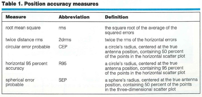
The original article showed how to derive a table like TABLE 1. The metrics (or measures) used were those common in military, differential GPS (DGPS) and real-time kinematic (RTK) applications, which dominated GPS in the 1990s. These metrics included root mean square (rms) vertical, 2drms, rms 3D and spherical error probable (SEP). The article showed examples from DGPS data.
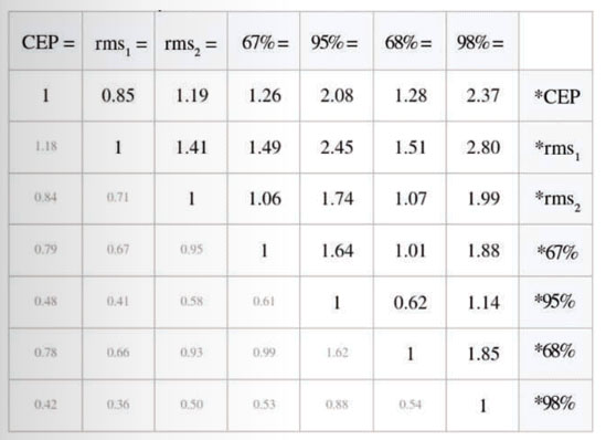
Table 1. Accuracy measures for circular, Gaussian, error distributions.Figure 1. Using Table 1.
Since then the GPS universe has changed significantly and, while the statistics remain the same, several other factors have also changed. Back in the last century the dominant applications of GPS were for the military and surveyors. Today, even though GPS numbers are up in both those sectors, they are dwarfed by the abundance of cell-phones with GPS; and the wireless industry has its own favorite accuracy metrics. Also, Selective Availability was active back in 1998, now it is gone. And finally we have the prospect of a 60+ satellite constellation, as we fully expect in the next nine years that 30 Galileo satellites will join the GPS and satellite-based augmentation systems (SBAS) satellites already in orbit.
Therefore, we take an updated look at GNSS accuracy.
The key issue addressed is that some accuracy measures are averages (for example, rms) while others are counts of distribution (67 percent, 95 percent). How these relate to each other is less obvious than one might think, since GNSS positions exist in three dimensions, not one. Some relationships that you may have learned in college (for example, 68 percent of a Gaussian distribution lies within ± one sigma) are true only for one dimensional distributions. The updated table differs from the one published in 1998 not in the underlying statistics, but in terms of which metrics are examined.
Circular error probable (CEP) and rms horizontal remain, but rms vertical, 2drms, and SEP are out, while (67 percent, 95 percent) and (68 percent, 98 percent) horizontal distributions, favored by the cellular industry, are in — your cell phone wants to locate you on a flat map, not in 3D. Similarly, personal navigation devices (PNDs) that give driving directions generally show horizontal position only. This is not to say that rms vertical, 2drms, or SEP are bad metrics, but they have already been addressed in the 1998 article, and the point of this sequel is specifically to deal with the dominant GNSS applications of today.
Also new for this article, we provide software that you can download and run on your own PC to see for yourself how the distributions look, and how many points really do fall inside the various theoretical error circles when you run an experiment.
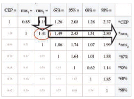
Table 1 is the central feature of this article. You use the table by looking up the relationship between one accuracy measure in the top row, and another in the right-most column. For example (see FIGURE 1), let’s take the simplest entry in the table: rms2 = 1.41× rms1
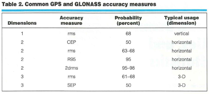
TABLE 2 defines the accuracy measures used in this article.
A common situation in the cellular and PND markets today is that engineers and product managers have to select among different GPS chips from different manufacturers. (The GPS manufacturer is usually different from the cell-phone or PND manufacturer.) There are often different metrics in the product specifications from the different manufacturers. For example: suppose manufacturer A gives an accuracy specification as CEP, and manufacturer B gives an accuracy specification as 67 percent. How do you compare them? The answer is to use Table 1 to convert to a common metric. Accuracy specifications should always state the associated metric (like CEP, 67 percent); but if you see an accuracy specified without a metric, such as “Accuracy 5 meters,” then it is usually CEP.
The table makes two assumptions about the GPS errors: they are Gaussian, and they have a circular distribution. Let’s discuss both these assumptions.
Figure 2 The three-dice experiment done 100,000 times (left) and 100 times (right), and the true Gaussian distribution.
Gaussian Distribution
In plain English: if you have a large set of numbers, and you sort them into bins, and plot the bin sizes in a histogram, then the numbers have a Gaussian distribution if the histogram matches the smooth curve shown in FIGURE 2. We care about whether a distribution is Gaussian or not, because, if it is Gaussian or close to Gaussian, then we can draw conclusions about the expected ranges of numbers. In other words, we can create Table 1. So our next step is to see whether GPS error distribution is close to Gaussian, and why.
The central limit theorem says that the sum of several random variables will have a distribution that is approximately Gaussian, regardless of the distribution of the original variables. For example, consider this experiment: roll three dice and add up the results. Repeat this experiment many times. Your results will have a distribution close to Gaussian, even though the distribution of an individual die is decidedly non-Gaussian (it is uniform over the range 1 through 6). In fact, uniform distributions sum up to Gaussian very quickly.
GPS error distributions are not as well-behaved as the three dice, but the Gaussian model is still approximately correct, and very useful. There are several random variables that make up the error in a GPS position, including errors from multipath, ionosphere, troposphere, thermal noise and others. Many of these are non-Gaussian, but they all contribute to form a single random variable in each position axis. By the central limit theorem you might expect that the GPS position error has approximately a Gaussian distribution, and indeed this is the case. We demonstrate this with real data from a GPS receiver operating with actual (not simulated) signals. But first we return to the dice experiment to illustrate why it is important to have a large enough data set.
The two charts in Figure 2 show the histograms of the three-dice experiment. On the left we repeated the experiment 100,000 times. On the right we used just the first 100 repetitions. Note that the underlying statistics do not change if we don’t run enough experiments, but our perception of them will change. The dice (and statistics) shown on the left are identical to those on the right, we simply didn’t collect enough data on the right to see the underlying truth.
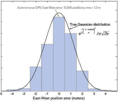
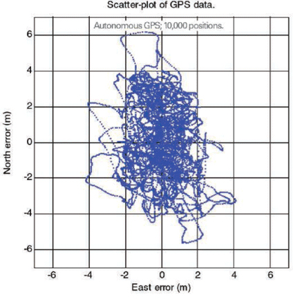
FIGURE 3 shows a GPS error distribution. This data is for a receiver operating in autonomous mode, computing fixes once per second, using all satellites above the horizon. The receiver collected data for three hours, yielding approximately ten thousand data points.
Figure 3. Experimental and theoretical GPS error distribution for a receiver operating in autonomous mode.
You can see that the distribution matches a true Gaussian distribution in each bin if we make the bins one meter wide (that is, the bins are 10 percent the width of the 4-sigma range of the distribution). Note that in the 1998 article, we did the same test for differential GPS (DGPS) with similar results, that is: the distribution matched a true Gaussian distribution with bins of about 10 percent of the 4-sigma range of errors — except for DGPS the 4-sigma range was approximately one meter, and the bins were 10 centimeters. Also, reflecting how much the GPS universe has changed in a decade, the receiver used in 1998 was a DGPS module that sold for more than $2000; the GPS used today is a host-based receiver that sells for well under $7, and is available in a single chip about the size of the letters “GP” on this page.
Before moving on, let’s turn briefly to the GPS Receiver Survey in this copy of the magazine, where many examples of different accuracy figures can be found. All manufacturers are asked to quote their receiver accuracy. Some give the associated metrics, and some do not. Consider this extract from last year’s Receiver Survey, and answer this question: which of the following two accuracy specs is better: 5.1m horiz 95 percent, or 4m CEP?
In Table 1 we see that CEP=0.48 × 95 percent. So 5.1 meters 95 percent is the same as 0.48× 5.1m = 2.4 meters CEP, which is better than 4 meters CEP.
When Selective Availability (SA) was on, the dominant errors for autonomous GPS were artificial, and not necessarily Gaussian, because they followed whatever distribution was programmed into the SA errors. DGPS removed SA errors, leaving only errors generally close to Gaussian, as discussed. Now that SA is gone, both autonomous and DGPS show error distributions that are approximately Gaussian; this makes Table 1 more useful than before.
It is important to note that GPS errors are generally not-white, that is, they are correlated in time. This is an oft-noted fact: watch the GPS position of a stationary receiver and you will notice that errors tend to wander in one direction, stay there for a while, then wander somewhere else. Not-white does not imply not-Gaussian. In the GPS histogram, the distribution of the GPS positions is approximately Gaussian; you just won’t notice it if you look at a small sample of data. Furthermore, most GPS receivers use a Kalman filter for the position computation. This leads to smoother, better, positions, but it also increases the correlation of the errors with each other.
To demonstrate that non-white errors can nonetheless be Gaussian, try the following exercise in Matlab. Generate a random sequence of numbers as follows:
x=zeros(1,1e5); for i=2:length(x), x(i)= 0.95*x(i-1)+0.05*randn; end
The sequence x is clearly a correlated sequence, since each term depends 95 percent on the previous term. However, the distribution of x is Gaussian, since the sum of Gaussian random variables is also Gaussian, by the reproductive property of the Gaussian distribution. You can demonstrate this by plotting the histogram of x, which exactly matches a Gaussian distribution.
In some data sets you may have persistent biases in the position. Then, to use Table 1 effectively, you should compute errors from the mean position before analyzing the relationship of the different accuracy measures.
Distributions and HDOP
Table 1 assumes a circular distribution. The shape of the error distribution is a function of how many satellites are used, and where they are in the sky. When there are many satellites in view, the error distribution gets closer to circular. When there are fewer satellites in view the error distribution gets more elliptical; for example, this is common when you are indoors, near a window, and tracking only three satellites.
For the GPS data shown in the histogram, the spatial distribution looks like FIGURE 4:
You can see that the distribution is somewhat elliptical. The rms North error is 2.1 meters, the rms East error is 1.2 meters. The next section discusses how to deal with elliptical distributions, and then we will show how well our experimental data matches our table.
Figure 4. Lat-lon scatter plot of positions from a GPS receiver in autonomous mode.
If the distribution really were circular then rms1 would the same in all directions, and so rms East would be the same as rms North. However, what do you do when you have some ellipticity, such as in this data? The answer is to work with rms2 as the entry point to the table. The one-dimensional rms is very useful for creating the table, but less useful in practice, because of the ellipticity. Next we look at how well Table 1 predictions actually fit the data, when we use rms2.
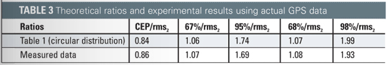
TABLE 3 shows the theoretical ratios and experimental results of the various percentile distributions to horizontal rms. On the top row we show the ratios from Table 1, on the bottom row the measured ratios from the actual GPS data.
Table 3. Theoretical ratios and experimental results using actual GPS data.
For our data: horizontal rms = rms2 = 2.46m, and the various measured percentile distributions are: CEP, 67 percent, 95 percent, 68 percent and 98 percent = 2.11, 2.62, 4.15, 2.65, and 4.74m respectively.
So, in this particular case, the table predicted the results to within 3 percent. With larger ellipticity you can expect the table to give worse results. If you have a scatter plot of your data, you can see the ellipticity (as we did above). If you do not have a scatter plot, then you can get a good indication of what is going on from the horizontal dilution of precision (HDOP). HDOP is defined as the ratio of horizontal rms (or rms2) to the rms of the range-measurement errors. If HDOP doubles, your position accuracy will get twice as bad, and so on. Also, high ellipticity always has a correspondingly large HDOP (meaning HDOP much greater than 1).
Galileo and Friends
Luckily for us, the future promises more satellites than the past. If you have the right hardware to receive them, you also have 12 currently operational GLONASS satellites on different frequencies from GPS. Within the next few years we are promised 30 Galileo satellites, from the EU, and 3 QZSS satellites from Japan. All of these will transmit on the same L1 frequency as GPS. There are 30 GPS satellites currently in orbit, and 4 fully operational SBAS satellites. Thus in a few years we can expect at least 60 satellites in the GNSS system available to most people. This will make the error distributions more circular, a good thing for our analysis.
Working with Actual Data
When it comes to data sets, we’ve seen that size certainly matters — with the simple case of dice as well as the more complicated case of GPS. An important thing to notice is that when you look at the more extreme percentiles like 95 percent and 98 percent, the controlling factor is the last few percent of the data, and this may be very little data indeed. Consider an example of 100 GPS fixes. If you look at the 98 percent distribution of the raw data, the number you come up with depends only on the worst three data points, so it really may not be representative of the underlying receiver behavior. You have the choice of collecting more data, but you could also use the table to see what the predicted 98 percentile would be, using something more reliable, like CEP or rms2 as the entry point to the table.
Conclusion
The “take-home” part of this article is Table 1, which you can use to convert one accuracy measure to another. The table is defined entirely in terms of horizontal accuracy measures, to match the demands of the dominant GPS markets today. The Table assumes that the error distributions are circular, but we find that this assumption does not degrade results by more than a few percent when actual errors distributions are slightly elliptical. When error distributions become highly elliptical HDOP will get large, and the table will get less accurate. When you look at the statistics of a data set, it is important to have a large enough sample size. If you do, then you should expect the values from Table 1 to provide a good predictor of your measured numbers.
Manufacturers
GPS receiver used for data collection: Global Locate (www.globallocate.com) Hammerhead single-chip host-based GPS.
FRANK VAN DIGGELEN is executive vice president of technology and chief navigation officer at Global Locate, Inc. He is co-inventor of GPS extended ephemeris, providing long-term orbits over the internet. For this and other GPS inventions he holds more than 30 US patents. He has a Ph.D. E.E. from Cambridge University.
“There are three kinds of lies: lies, damn lies, and statistics.” So reportedly said Benjamin Disraeli, prime minister of Great Britain from 1874 to 1880. And just as the notoriously wily statesman noted, the science of analyzing data, or statistics, sometimes yields results that one can interpret in a variety of ways, depending on politics or interests. Likewise, we in the satellite navigation field interpret results depending on the information we wish to produce: Using various statistical methods, we can create many different GPS and GLONASS position accuracy measures. It can seem confusing, even misleading, but as we’ll see in this month’s column, there’s some rhyme to our reason. We’ll examine some of the most commonly used accuracy measures, reveal their relationships to one another, and correct several common misconceptions about accuracy. Our author is Frank van Diggelen of Ashtech, Inc., in Sunnyvale, California. Van Diggelen is the OEM (original equipment manufacturer) and navigation products marketing manager.
“Innovation” is a regular column featuring discussions about recent advances in GPS technology and its applications as well as the fundamentals of GPS positioning. The column is coordinated by Richard Langley of the Department of Geodesy and Geomatics Engineering at the University of New Brunswick, who appreciates receiving your comments as well as topic suggestions for future columns.
Root mean square (rms), twice the distance root mean square (2drms), circular error probable (CEP), spherical error probable (SEP), so on, and so forth — Why do we have so many different position accuracy measures? The answer lies in the fact that the errors of position coordinates determined using a GPS or GLONASS unit are not constant — they vary statistically. If you observe the reported position of a stationary receiving system over time, you will notice it wanders. Graphing these moving points yields a “scatter plot”; how you analyze the scatter depends on the information you want to obtain. To complicate matters, the position is fundamentally three dimensional, but not everyone is interested in obtaining three-dimensional accuracy. One user might care about horizontal accuracy, another might want vertical. Thus, clearly, we must consider different accuracy measures.
Before we take a look at some of the common accuracy evaluations and their relationships to one another, we must say a word about the meaning of accuracy itself. To ascertain how accurately a system has determined a point’s coordinates, you must know the point’s true coordinates. Typically, this comes from measurements made using a system with an inherently higher accuracy than the one being tested. Simply averaging a system’s reported positions will provide an indication of system precision or repeatability, but the measurements might contain a bias that could affect the results. So, when we talk about system accuracy, we must consider the possibility of such a mean error.
POPULAR ACCURACY MEASURES
Table 1 lists the most commonly used GPS position accuracy measures and their definitions. Note that the first two methods are explained in terms of average squared error, and the last three are defined directly from the position error distribution (the scatter). Thus, we can immediately associate these last three with error probabilities. If we assume that the error distribution along any axis (east, north, or up) is “normal” or Gaussian, then we can also derive probabilities associated with the rms and 2drms accuracy measures. [The normal or Gaussian distribution is the one to which the dispersion of the sum of a very large number of very small errors always converges. The famous German polymath Carl Friedrich Gauss used this distribution to develop his error theory in the early nineteenth century. To honor the importance of this and the scientist’s other accomplishments, Germany features a portrait of Gauss and his probability distribution on its 10-mark bank note. — R.B.L.]
Data: Frank van Diggelen
Table 2 shows how the accuracy measures are used and what probabilities can be associated with them. Note that the probability associated with rms depends on whether one is using rms in one, two, or three dimensions (1-D, 2-D, or 3-D). The later “Common Misconceptions” section discusses this further.
Data: Frank van Diggelen
Ascertaining Accuracy: An Example. Now, suppose you are comparing the specifications of two positioning systems. One unit has a quoted accuracy of 3 meters (3-D rms) and another has a quoted accuracy of 2 meters (CEP). Which system is more accurate?
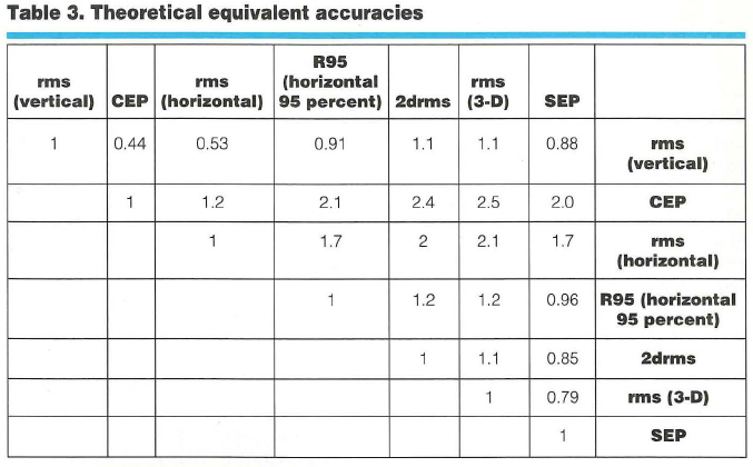
By making three assumptions about the ratio of east, north, and up errors, we can relate different accuracy determinations to each other, as shown in Table 3 (entitled “Theoretical Equivalent Accuracies”).To use that table, identify the desired measure in the top row and the original measure in the right hand column. Take the number in the cell at which the row and column intersect and multiply it by the original measure value to yield the desired number.
Data: Frank van Diggelen
The three assumptions, from which the conversion values derive, are true on average. First assumption, the error distribution is Gaussian. Second, the ratios of the position dilution of precision (PDOP) to the horizontal DOP (HDOP) and the vertical DOP (VDOP) to the HDOP are 2.1:1 and 1.9:1, respectively. Third, the horizontal error distribution is circular. These suppositions are based on simulations performed over a grid covering the entire globe between latitudes 66 degrees south and 66 degrees north. In general, horizontal distributions are elliptical, the ellipses are often very close to circular, and the circular Gaussian distribution model is very good at estimating the true distribution, as shown in Figure 1.
To answer the question posed earlier (which is more accurate — a 2-meter [CEP] or a 3-meter [3-D rms] system?), follow these four steps:
Go down the “rms (3-D)” column to the “CEP” row.
The entry in this cell is 2.5.
According to the table, rms (3-D) =2.5 3 CEP.
So, CEP = rms (3-D)/2.5 = 3/2.5 =1.2 meters.
Thus, a system with 3-D rms of 3 meters will have a CEP of 1.2 meters and is, therefore, more accurate than a system with a CEP of 2 meters.
For specific details about how we created Table 3, see the “Deriving the Equivalent Accuracies Table” sidebar on the last page of this article.
Making Valid Assumptions. To understand the table in more general terms, one must realize that the three assumptions and the table are valid for the average measurement. This means that if someone takes measurements all day, then, on average, the different accuracies are related by the numbers in the table. At any instant, however, the satellite geometry may produce a different relationship between various accuracies (for example, between vertical and horizontal). But the best way to make a comparison, seemingly, is to use average relationships.
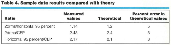
Starting a Small Test. In any specific example, the table entries are apparently good to within 620 percent. That is, if the table says 2drms = 1.2 3 horizontal 95 percent, then a particular experiment may show 2drms to be anywhere from 0.96 to 1.44 3 horizontal 95 percent.
To evaluate Table 3’s efficacy, we used data from more than 550 hours (2 million data points) of differential GPS positions (DGPS), obtained with a U.S. Coast Guard reference station providing the differential corrections. Our results were 42 centimeters CEP, 91 centimeters horizontal 95 percent, and 104 centimeters 2drms. Table 4 shows how these results compare with Table 3’s theoretical values.
Data: Frank van Diggelen
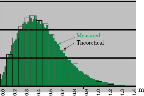
Closing the Circle. The circular Gaussian distribution model for horizontal errors is surprisingly good. Figure 1 portrays a histogram (in green) generated from the DGPS data. These data have a horizontal rms value of 0.52 meter. Overlaid on the green histogram is a bar graph, showing the theoretical histogram that would be obtained from data that truly were circularly distributed and Gaussian and that had the same horizontal rms as the measured data. As the figure shows, the measured and theoretical distributions agree extremely well. We can obtain similarly good fits for vertical error distributions modeled as 1-D Gaussian.
Figure 1. Measured and theoretical horizontal error distribution. The vertical axis indicates the relative frequency of errors occurring in each error interval. Horizontal axis values are rounded. (Data: Frank van Diggelen)
COMMON MISCONCEPTIONS
By now, one may feel that accuracy measures are rather simple to understand. Still, general discussions about GPS and GLONASS position accuracies frequently contain several misconceptions. Here’s our attempt to set the record straight.
Misconception Number 1 — rms precisely equals one sigma (1s or 1 standard deviation). Well, actually this is true, as long as the mean error is zero. With most GPS or GPS/GLONASS systems, the mean errors (over a sufficiently long time interval) are zero, or close to zero, and so rms may be considered essentially equivalent to one sigma.
Misconception Number 2 — 2drms means “two-dimensional rms.”In fact, 2drms usually stands for “twice distance rms,” in which the “distance” is measured in a 2-D space, the horizontal plane. Thus, 2drms is a very confusing abbreviation: It is a two-dimensional measure, but the “2d” usually stands for twice distance. (Some publications about navigation accuracies, notably those issued by the North Atlantic Treaty Organization, use the alternative meaning of “2d.” Thus, their “2drms” is exactly one-half of the usual measure.)
Misconception Number 3 — 2drms is exactly equivalent to a 95 percent probability level. This untrue belief stems from the fact that, for a 1-D Gaussian distribution, 95 percent of it lies inside an interval from 2s to +2s. However, 2drms is a measure for a 2-D distribution. The percentage of scatter lying within a circle with radius equal to 2drms depends on the distribution shape. For a circular distribution, the percentage of scatter inside a 2drms circle is 98 percent. The “Deriving the Equivalent Accuracies Table” sidebar shows this. As the scatter becomes more elliptical (with different error distributions for the two horizontal coordinates), it also becomes more one-dimensional, causing the percentage of elliptical distribution values inside a 2drms circle to tend toward 95 percent.
For GPS units, when the whole sky is visible above a 10-degree mask angle, scatter is approximately circular. Typically, distributions become very elliptical when HDOP gets large (much greater than 1). Thus, for any GPS receiver in any environment, the circle with a radius equal to 2drms contains between 95 and 98 percent of the scatter. When HDOP is low, the percentage is closer to 98 percent; when HDOP is high, it is closer to 95 percent.
Misconception Number 4 — rms is perfectly comparable with a 68 percent probability level. This is true for only 1-D Gaussian distributions. For 2-D or 3-D Gaussian distributions, the percentage of the values distributed inside a circle (or sphere), with a radius equal to the rms value, depends on distribution shape.
Misconception Number 5 — The error distribution really is Gaussian.We use the assumption that the error distribution is Gaussian for analytical purposes, and over time, one can show that a circular Gaussian distribution can model the errors very well (see Figure 1). However, certain errors may not have a Gaussian distribution:
Stand-alone GPS errors are dominated by selective availability. Because this is an artificial error source, the errors it contributes are not always Gaussian.
Stand-alone GPS/GLONASS errors show distributions that match Gaussian distributions quite well (to about 10 percent) over a time period of, say, several hours.
Differential errors over a long time
display distributions that match Gaussian patterns to within a few percent. This is true for both code differential and carrier-phase differential (commonly referred to as real-time kinematic, or RTK). Differential errors over a short time produce scatter dominated by multipath, which is fairly constant over a few minutes, and, hence, the distribution is distinctly non-Gaussian.
IN CONCLUSION
As Disraeli also noted, “An investment in knowledge pays the best interest.” We hope that this brief note has proven to be a worthwhile “investment” to readers, shedding light on the sometimes murky subject of accuracy measures used in GPS and GLONASS positioning. With the simple information provided, you should be able to compute the positioning accuracy of a system in a variety of measures and also, contrary to the old adage, be able to compare “apple A” with “orange B.”
Further Reading
For an introduction to the statistics of GPS accuracy measures, see
“The Mathematics of GPS,” by R.B. Langley in GPS World, Vol. 2, No. 7, July/August 1991, pp. 4550.
For an extended mathematical description of position errors, see
“Navigation Errors,” Appendix Q of American Practical Navigator: An Epitome of Navigation, originally by N. Bowditch, Vol. I, published by the former Defense Mapping Agency Hydrographic Center, Washington, D.C., 1977 or 1984 editions.
For positional error discussions from the war fighter’s perspective (but also relevant to noncombat applications), see
“Accuracy and Positional Error,” Appendix D of Naval Aviation Systems Team Mapping, Charting, and Geodesy Handbook, Version 2.0, by J.H. Harden, Jr., and Z.S. Willis, published by the Avionics Systems Engineering Department, Naval Air Systems Command, Arlington, Virginia, 1995. Available on the Internet at <http://www.nima.mil/publications/pub.html>.
‘Method of Expressing Navigation Accuracies,” NATO Standardization Agreement (STANAG) 4278, Edition 2, Military Agency for Standardization, North Atlantic Treaty Organization Headquarters, Brussells, 1986.
For an advanced discussion about the statistics of GPS positioning errors, see
“Random Variables and Covariance Matrices,” Chapter 9 of Linear Algebra, Geodesy, and GPS, by G. Strang and K. Borre, Wellesley-Cambridge Press, Wellesley, Massachusetts, 1997.
Deriving the Equivalent Accuracies Table
The function invchisq (p,2) computes the square of a circle’s radius such that the sum of squares of two random variables, each with rms = 1s = 1, has a probability p of falling inside the circle. This function allows users to relate rms to probability for a two-dimensional circular distribution.Comments are shown in curly brackets “{}.” Table 3 (about equivalent accuracy) contains entries with resolution of only two digits. It is impossible, in general, to provide more precise ratios, because the three initial assumptions are averages over the whole world, and, thus, are good only to within a few percent of error in any particular region.rms (vertical) = 1.9 3 rms (horizontal) {using VDOP/HDOP = 1.9}
(1,3) entry = 1/1.9 = 0.53
(1,5) entry = 2 3 0.53 = 1.1CEP = 50 percent circle {first solve for CEP = x 3 rms (horizontal), then use that result to derive other ratios}
rms (horizontal) = (check)2 3 rms (linear) {assuming a circular distribution}
R = sqrt(invchisq ( 0.5,2)) = 0.83 3 (check)2 => CEP = 0.83 3 (check)2 3 rms (linear) = 0.83 3 rms (horizontal)
(2,3) entry = 1/0.83 = 1.2
CEP = x 3 rms (vertical) = x 3 rms (horizontal) 3 1.9 = 0.83 3 rms (horizontal) => x = 0.83/1.9 = 0.44
(1,2) entry = 0.44R95 = 95 percent circle {first solve for R95 = x 3 rms (horizontal), then use that result to derive other ratios]
R = sqrt(invchisq (0.95,2)) = 1.73 3 (check)2 =>
R95 = 1.73 3 (check)2 3 rms (linear) = 1.73 3
rms (horizontal)(3,4) entry = 1.7R95 = x 3 rms (vertical) = x 3 rms (horizontal) 3 1.9 = 1.73 3 rms (horizontal) => x = 1.73/1.9 = 0.91
(1,4) entry = 0.91R95 = 1.73 3 rms (horizontal) = 1.73 3 CEP/0.83
(2,4) entry = 1.73/0.83 = 2.1
2drms = 2 3 rms (horizontal) {by definition}
(3,5) entry = 22drms = x 3 CEP = x 3 0.83 3 rms (horizontal) =
x 3 0.83 3 2drms/2 => x = 2/0.83 = 2.4
(2,5) entry = 2.42drms = x 3 R95 = x 3 1.73 3 rms (horizontal) = x 3 1.73 3 2drms/2 => x = 2/1.73 = 1.16
(4,5) entry = 1.2