A Tidal Shift
Traditional tide gauges are in contact with the water surface and as a result are susceptible to measurement error and damage during extreme weather. An alternative approach is the use of GNSS reflectometry. We learn how this innovative use of satellite navigation signals works in this month’s Innovation column.

Seawater level is conventionally monitored by tide gauges that measure the vertical distance of the water surface from a point on the ground. As the tide gauges provide seamless and highly accurate measurements, many countries operate a tide-gauge network to monitor sea-level changes and to assess flood risk. For example, the National Oceanic and Atmospheric Administration (NOAA) operates a permanent observing system, the National Water Level Observation Network (NWLON), with more than 400 gauges throughout the United States.
However, some challenges of tide gauges can be identified. Firstly, tide-gauge measurements require direct contact with the water, which causes limitations in installing and maintaining the equipment. The equipment requiring direct sensing is highly vulnerable to coastal hazards, such as coastal flooding and tsunamis, resulting in potential measurement errors or even equipment destruction during severe natural events.
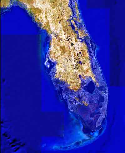
Furthermore, tide gauges require maintenance on a regular basis, which is expensive because it requires the use of divers. This greatly limits the operation of tide gauges, especially in extreme environments such as in the Arctic. Alaska, for example, has significant gaps in its available spatially-varying tidal information. However, in the Arctic, it is also very important to constantly and closely monitor the long- and short-term variation of water levels because this area has a significant impact on global climate and ecosystems. Consequently, more support is needed for sea-level monitoring and coastal mapping in this region.
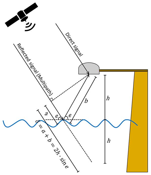
GNSS can serve as an alternative approach for water-level monitoring. GNSS satellites continuously transmit radio signals and ground-based, space-based, and airborne receivers access the signals regardless of weather conditions. Some of the received signals are reflected from obstacles or surfaces near the antenna, a phenomenon referred to as multipath (see FIGURE 1).
Multipath tends to be regarded as one of the major error sources for GNSS positioning where it causes unexpected phase delays when compared to the direct signal. Consequently, various procedures have been developed to mitigate the multipath effect. However, the GNSS signals reflected from the Earth’s surface contain information about the geophysical properties of the reflecting surface. The use of these signals is known as GNSS reflectometry (GNSS-R). GNSS-R allows us to monitor the temporal variation of water levels by calculating phase delays of GNSS signals reflected from the water surface. A GNSS-R-based tide gauge does not require direct contact with the water because it measures the water levels based on a remote-sensing technique. Thus, a GNSS-R-based tide gauge can be effectively applied to water-level monitoring.
However, several challenges exist in processing GNSS signals observed at high latitudes compared to mid-latitudes. Not only do we have to contend with extreme weather conditions and limited infrastructure availability, but also with problematic satellite geometry and ionospheric effects on the GNSS signals. To overcome these limitations in the use of GNSS-R in the Arctic, we introduce enhanced algorithms to improve the temporal and spatial resolutions of GNSS-R sea-level measurements.
Our approach includes an enhanced spectrum analysis based on multi-frequency signals and statistical reliability verification. Moreover, we include the signals transmitted by the Galileo constellation in addition to GPS to improve the quantity and the quality of GNSS observations in the Arctic. We have tested the proposed method with an experiment in Alaska and validated the results with nearby tide gauges. The experimental results clearly show the feasibility of employing GNSS-R-based tide gauges in the Arctic.
GNSS-R-BASED WATER-LEVEL MONITORING
Martin-Neria first introduced a method of monitoring sea level using the GNSS-R technique in 1993. Thereafter, many studies have been conducted to apply GNSS-R to water level estimation. Anderson proposed a method to estimate sea level using the interference pattern caused by the direct and reflected GNSS signals, which relies on the fact that the spacing between peaks in the interference pattern is almost entirely dependent on the height of the antenna above the reflecting surface.
The phase difference in the GNSS receiver between the direct and the reflected satellite signals varies while the geometry of a GNSS satellite changes (see Figure 1), generating the interference pattern. The interference pattern is particularly noticeable in signal-to-noise ratio (SNR) data. The reflected signals contribute to the SNR data in the form of oscillations, while the smoothly rising overall arc mostly depends on the signal strength and the antenna gain pattern.
The reflected signals can be isolated from the SNR data by removing the main trend — for example, by polynomial fitting — indicative of the direct signal. The frequency of the remaining dSNR oscillations is constant with respect to the sine of the elevation angle, assuming that the water level does not change during the satellite arc and the reflection surface is horizontal. Consequently, the frequency of the oscillation is linearly proportional to the height of the antenna above the reflecting surface.
The frequency can be derived from the dSNR data by spectral analysis. Among a number of spectral-analysis methods, the Lomb-Scargle periodogram (LSP) is commonly applied since it allows for processing of unevenly sampled data.
Determining the frequency of the oscillations. The antenna height above the water surface is directly calculated from the frequency of the oscillations derived from LSP processing. However, it is difficult to determine the dominant frequency because of the roughness of the water surface, especially in extreme environments such as Arctic regions with high currents and strong winds. In addition, the observed SNR data is easily affected by obstacles near the GNSS antenna. Therefore, it is difficult to distinguish the spectral peak of the signal reflected from the water surface from other additional reflected signals, especially when additional and unexpected reflections occur near the sea surface.
To minimize the erroneous determination of the frequency of the oscillations using dSNR, we can take advantage of the multiple frequencies of modern GNSS signals. In our study, we processed signals from both the GPS and Galileo constellations, with GPS transmitting three carrier signals (L1, L2 and L5) and Galileo transmitting five carrier signals (E1, E5a, E5b, E5ab and E6).
By comparing the spectrum peaks from the multiple signals on different frequencies, one can analyze the dominant peaks across the different frequencies on the same raypath. This algorithm is based on the fact that the multiple frequency signals should detect consistent sea-level heights because they are transmitted along the same raypath during the same period. One of the biggest advantages of this approach is that no additional data or equipment is required to accurately determine the frequency of oscillations of the GNSS signals reflected from the water surface.
Statistical Testing of Retrieved Sea Levels. Reflected signals are not necessarily all from the sea surface. To remove erroneous solutions, we conducted a statistical test. Data including measurement errors and/or some noise can be approximated to the model by the least squares method that determines the model parameters by minimizing the sum of squared residuals. However, this method yields an incorrect result when many outliers deviating from the normal distribution are included in the data set.
This problem can be overcome by applying RANdom SAmple Consensus (RANSAC). RANSAC stochastically estimates the model parameters maximizing consensus, that is, the parameter supported by the largest number of sample data through an iterative process. However, the RANSAC results can act differently each time for the same input data because it is essentially a statistical estimation method using random samples. Therefore, we perform RANSAC with rough constraints primarily to remove outliers significantly out of normal range, then the remaining noise in the data can be excluded by performing secondary fitting using tightly constrained least squares. For the least squares procedure, a series was applied for the fitting model, which represents various motions of the sea surface such as ocean tide loading, as a sum of trigonometric functions.
SEA-LEVEL MONITORING IN ST. MICHAEL
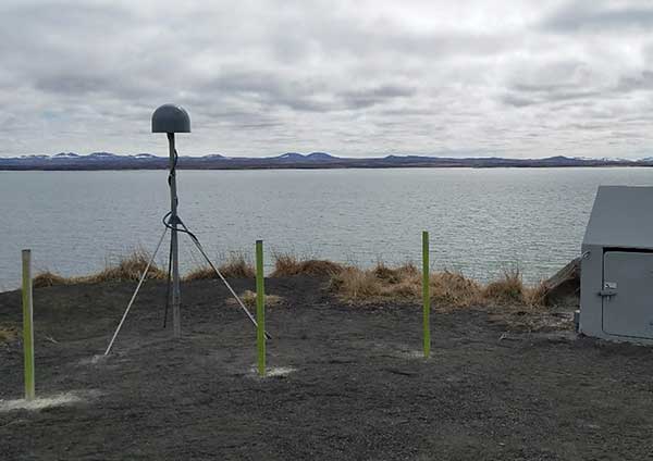
The Plate Boundary Observatory (PBO) network operated by UNAVCO (formerly the University NAVSTAR Consortium) is primarily designed to monitor long-term tectonic and volcanic deformation. However, it can also be used for GNSS-R applications. A new PBO station, AT01, was installed in May 26, 2018, in St. Michael, Alaska, which is designed to be suitable as a GNSS-R-based tide gauge with a clear and wide-open view toward the sea covering from 0° to 230° in azimuth (see FIGURE 2). The equipment at this site consists of a Trimble choke-ring geodetic antenna and a Septentrio PolaRx5 receiver that can receive not only GPS signals but also those of Galileo, with data recorded every 15 seconds.
We have used this station to assess our technique using one month of SNR data from June 2018. It should be emphasized that not only GPS but also Galileo signals were processed, and the Center for Orbit Determination in Europe’s Multi-GNSS Experiment final orbit and satellite clock products were used to minimize the satellite orbit error. Additionally, NOAA tide gauge stations (9468132 and 9468333) were used for comparison and verification of the water levels measured from the GNSS-R-based tide gauge (see FIGURE 3).
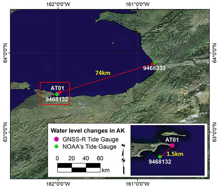
The 9468132 tide gauge in St. Michael is the nearest tide gauge at approximately 1.5 kilometers from AT01. However, since it is not operational, NOAA only provides water-level predictions (just high and low tides) based on the harmonic constituents, not the actual measurements. On the other hand, the 9468333 tide gauge in Unalakleet is approximately 74 kilometers away from AT01. This makes it difficult to use the tide gauge as ground truth, but it does provide the actual sea-level measurements including any abnormal daily variations during the observation period. Therefore, we used the water-level predictions and measurements from both stations to validate the GNSS-R-based water-level measurements at AT01.
Determination of Water Level. The GPS and Galileo SNR data were independently analyzed using our in-house software package (written in MATLAB) using the following procedures.
As a preprocessing step, each SNR data series was examined to filter out the signals reflected from other surfaces surrounding the antenna and to isolate the signals that were reflected by the sea surface. Since AT01 PBO station was installed to investigate the feasibility of its use as a GNSS-R-based tide gauge, the most effective azimuth and elevation ranges were given, which are 0° to 230° and 10° to 25°, respectively.
The azimuth and elevation angle ranges were applied, which effectively removed reflected signals from surfaces other than the sea surface. After identifying the SNR data affected by the reflection from the sea surface, the processing windows were dynamically determined by the continuous path and direction (ascending and descending) of the satellites, and the height of the sea surface was estimated using only a portion of the satellite arc contained within each processing window.
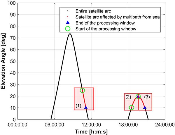
For example, FIGURE 4 shows the processing windows determined for the GPS satellite PRN 1 on June 1, 2018. The red dots in the figure show the parts of the satellite arcs affected by multipath from the sea surface. The data was divided into three processing windows due to the arc discontinuities and satellite path directions. It should be noted that only the processing windows with a data span of 30 minutes or longer were used for water level estimation. This minimum data span duration of 30 minutes was empirically determined by observing the probability of failure of the water -level calculation for shorter spans.
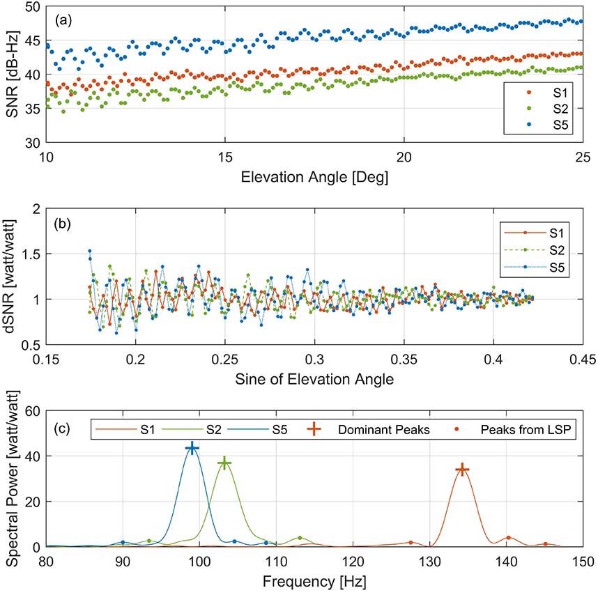
To isolate multipath effects from the SNR observation, we removed the trend in the SNR by a second-order polynomial fitting using only the portion of a satellite arc contained within each window. FIGURE 5 (b) shows the detrended SNR (dSNR) from FIGURE 5 (a), and the impact of the multipath is clearly identified in the form of the oscillation. As discussed earlier, the oscillation frequency is related to the antenna height above the sea surface. Accordingly, the dSNR data was analyzed through an LSP. As shown in FIGURE 5 (c), multiple peaks are founded from the LSP results of each dSNR series, and it is not easy to distinguish the frequency of the reflected signal from the sea level among these peaks.
Since multiple frequency signals from the same satellite must detect the same sea-level height, the final dominant peak was determined by checking the consistency of the resulting heights from each dominant peak among the multi-frequency signals. After that, the dominant frequency was converted to the antenna height above the reflection surface, which was then subtracted from the orthometric height of the antenna (the height above the geoid or, approximately, the height above mean sea level [MSL]) to refer the height of the instantaneous sea surface to MSL.
After analyzing all SNR data observed during one day, we carried out the reliability test of the retrieved sea levels to reject erroneous sea-level solutions.
RESULTS AND VALIDATION
The water-level changes from the GNSS-R-based tide gauge at St. Michael were compared to the independently predicted and measured sea levels from the neighboring St. Michael and Unalakleet tide gauges during June 1–30, 2018. Although the tide gauges are considered reliable ground truth, our experimental study must take into account the physical distance between the sites (about 1.5 and 74 kilometers from AT01, respectively) as well as the difference coming from the model versus the actual measurement.
In addition, a vertical offset between the data time series of the GNSS-R-based tide gauge and the standard tide gauges should be considered due to their different datums. Whereas the GNSS-R-derived sea level refers to a geodetic datum — namely the U.S. National Spatial Reference System (NAVD 88) — a standard tide gauge is highly localized with reference to a tidal datum such as local mean sea level. Generally, the difference between the geodetic and tidal datums is provided by NOAA, which allows us to convert between two vertical datums.
However, the vertical datum in Alaska has significant gaps in the spatially varying tidal information because of the difficulties of operating tide gauges there so that accurate information for datum conversion cannot be obtained. Therefore, the averages of the vertical differences were calculated (–6.44 centimeters for the St. Michael tide gauge and 9.54 centimeters for the Unalakleet tide gauge), which were then applied to each of the time series to make the comparisons. In fact, such a problem implies another advantage of a GNSS-R-derived tide gauge: it already returns a water-level height based on the terrestrial datum so that the datum of the land and the ocean can be consistently retained.
FIGURE 6 shows the sea level derived from the GNSS-based tide gauge measurements using GPS (red dots), Galileo (blue dots), the predicted sea level from the St. Michael tide gauge (green dots and lines) and measured sea level from the Unalakleet tide gauge (blue line).
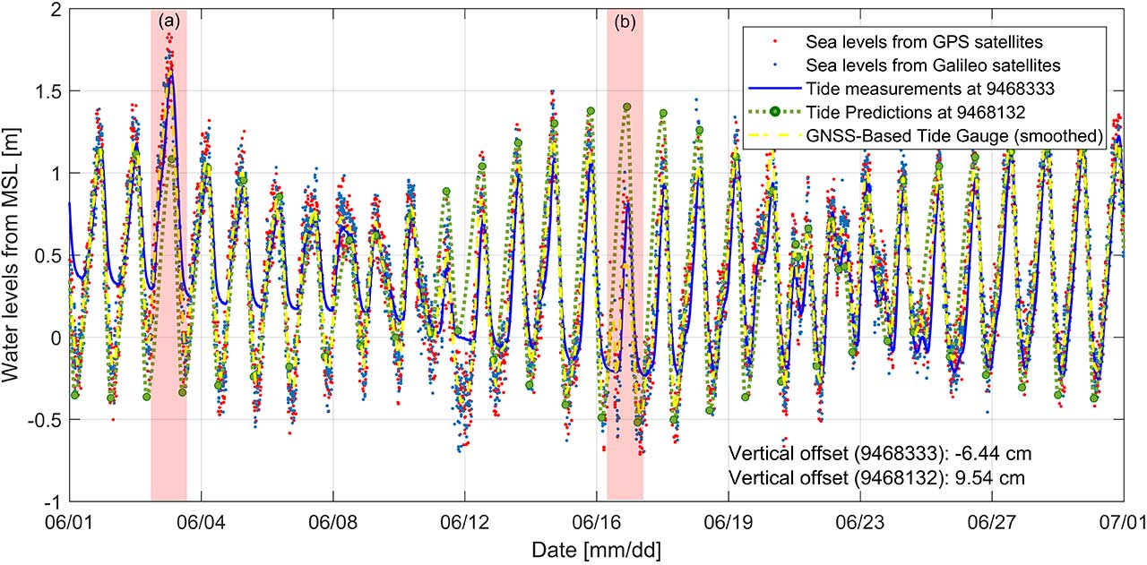
The overall results show good agreement with the tide predictions at the nearby St. Michael tide-gauge station. It should be noted that the St. Michael tide gauge only provides high- and low-tide predictions so these were interpolated. However, some tidal characteristics not represented in the published predictions were also confirmed. In particular, as shown in the red-shaded segments of the time series marked (a) and (b) in Figure 6, larger and lower amplitudes than the tide predictions for the St. Michael tide gauge were identified on June 3 and 16, respectively.
These inconsistencies can be explained by the comparison with actual sea-level measurements at the Unalakleet tide gauge (solid blue line in Figure 6), which show very similar sea-level changes compared to those of the GNSS-R-based tide gauge. In addition, the overall larger amplitudes in the time series from the Unalakleet tide gauge can be explained by considering the fact that the amplitudes of the water levels vary along the coastline in Alaska and the Unalakleet tide gauge is approximately 74 kilometers from AT01.
To quantitatively investigate the agreement between the GNSS-R-based tide gauge and the standard tide gauges, we computed correlation coefficients. To ensure simultaneous data, the standard tide-gauge measurements and predictions were interpolated to the time tags of the GNSS-R-based time series. The correlation coefficients are 0.87 and 0.81 with the St. Michael and Unalakleet tide gauges, respectively.
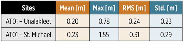
The statistical analysis of the comparison result is summarized in TABLE 1. The mean and maximum values were computed using the absolute sea-level differences. From the results, it could be established that the GNSS-R-derived sea level shows better agreement with actual sea-level measurements at the Unalakleet tide gauge even though it is approximately 74 kilometers away from AT01.
Spectral analysis was additionally conducted to validate the sea levels from the GNSS-R-based tide gauge. Because the St. Michael tide gauge does not provide actual measurements (only predictions), only the Unalakleet tide gauge was used in the spectral comparison. A fast Fourier transform (FFT) was applied to convert the time series of the sea levels to the frequency domain.
The GNSS-R-based tide gauge showed good agreement with the Unalakleet tide gauge overall. In addition, from the corresponding spectral analysis results, we were able to find meaningful harmonic constituents, M2, K1 and O1. The harmonic constituents estimated from the sea-surface measurements of the GNSS-R-based tide gauge have amplitudes most similar to the published harmonic constituents of the nearest St. Michael tide gauge, although the difference in amplitudes of the three harmonic constituents averages 12.3 centimeters.
In fact, the Unalakleet tide gauge also does not exactly match the amplitude of the estimated harmonic constituents and the published harmonic constituents. But by summarizing the corresponding results, we can conclude that the harmonic constituents estimated from the GNSS-R-based tide gauge are reliable.
As mentioned earlier, in our study, we estimated the water-level change by using GPS and Galileo satellite signals to overcome the degradation of GNSS performance due to the satellite geometry in the Arctic. The smoothed time series, calculated from a moving-average filter of two-hour intervals, is shown in Figure 6 (yellow dashed lines). The time series of sea level derived by the GNSS-R-based tide gauge during the whole month were used as ground truth for evaluating the accuracy.
This was done because the Unalakleet tide gauge is approximately 74 kilometers away from AT01 and the St. Michael tide gauge does not provide actual measurements, making it difficult to use as ground truth. As a result, the sea levels determined using the Galileo and GPS signals showed very similar accuracy with an average difference of 0.11 meters. Therefore, even if Galileo is additionally used, the estimated final water levels were at a similar level of accuracy.
However, the number of water-level observations dramatically increased (approximately doubled) when GPS and Galileo signals were both involved, even though the number of Galileo satellites is fewer than the number of GPS satellites. This is because Galileo transmits on five frequencies while GPS transmits on just three, so we can achieve more robust solutions by including Galileo.
We investigated how adding Galileo satellites changes the temporal resolution of the final sea-level measurements. At this time, several sea-level measurements pointing to the same epoch (such as sea levels from several frequency observations of the same satellite arc) were considered as one measurement for the time interval computation.
Overall, sea-level measurements using only Galileo satellites show lower temporal resolution compared to GPS satellites alone, with a mean time interval of 48.97 minutes because Galileo is not fully operational yet and fewer satellites are available. However, combining GPS and Galileo satellites to the sea-level analysis significantly increased the time resolution.
When only GPS satellites were used, the maximum time interval between two water-level measurements was greater than 3 hours, while the maximum time interval was shortened to about 1.5 hours when Galileo satellites were included in the water-level measurement.
However, even if both GPS and Galileo satellites were used, the average time interval was still 14.1 minutes, which is considerably longer than the time resolution of the standard tide gauge of 6 minutes. The lower time resolution of a GNSS-R-based tide gauge is explained by the limited ranges (azimuth and elevation angle ranges of 0° to 230° and 10° to 25°, respectively) toward the ocean at station AT01. It means the time resolution can be improved by securing a wider view of the ocean from the GNSS-R-based tide gauge.
SUMMARY AND CONCLUSION
The purpose of our study was to evaluate and verify the feasibility of using GNSS-R for sea-level monitoring in the Arctic. We used data from a GNSS station in St. Michael, Alaska, and applied an advanced algorithm that accurately determines sea levels through the comparisons of results from multiple GNSS signals along with an effective filtering procedure. Our results were validated through comparisons with measurements and predictions from nearby standard tide gauges.
From the corresponding analysis, we could confirm that the GNSS-R technique overcomes the limitations of standard tide gauges in the Arctic and successfully estimated the sea-level change in St. Michael, Alaska. The results from this study show many promising applications for a GNSS-R-based tide gauge in the Arctic, such as tsunami and flood monitoring and tidal datum determination.
In future studies, additional research should be conducted on how well the GNSS-R-based tide gauge can operate in extreme conditions such as low temperatures, wind gusts, storms, and snow. And, for further improvement of the temporal resolution of the technique, all active GNSS constellations including GPS, GLONASS, Galileo, and BeiDou should be included — that will certainly improve the temporal resolution and also potentially improve the accuracy and reliability. It would be also worth studying the spatial variations of sea-level changes by investigating the specular reflection points of GNSS multipath signals.
ACKNOWLEDGMENTS
This article is based on the paper “Monitoring Sea Level Change in the Arctic Using GNSS-Reflectometry” presented at ION ITM 2019, the 2019 International Technical Meeting of The Institute of Navigation, Reston, Virginia, Jan. 28–31, 2019.
SU-KYUNG KIM is a graduate research assistant at Oregon State University in Corvallis, Oregon. She received her M.Sc. in geoinformation engineering from Sejong University in Seoul, South Korea, in 2013. Her research interests are focused on sea-level change monitoring and crustal deformation studies using GNSS.
JIHYE PARK is an assistant professor of geomatics at Oregon State University. She holds a Ph.D. in geodetic science and surveying from The Ohio State University in Columbus, Ohio. Her research interests include GNSS positioning and navigation, GNSS reflectometry, ionospheric and tropospheric monitoring for natural hazards and artificial events, and other geospatial-related topics.
FURTHER READING
- Authors’ Conference Paper
“Monitoring Sea Level Change in the Arctic Using GNSS-Reflectometry” by S.-K. Kim and J. Park in Proceedings of ION ITM 2019, the 2019 International Technical Meeting of The Institute of Navigation, Reston, Virginia, Jan. 28–31, 2019.
- Pioneering Work by Manuel Martin-Neira
“The PARIS Concept: An Experimental Demonstration of Sea Surface Altimetry Using GPS Reflected Signals” by M. Martín-Neira, M. Caparrini, J. Font-Rossello, S. Lannelongue and C.S. Vallmitjana in IEEE Transactions on Geoscience and Remote Sensing, Vol. 39, No. 1, 2001, pp. 142–150, doi: 10.1109/36.898676.
“A Passive Reflectometry and Interferometry System (PARIS): Application to Ocean Altimetry” by M. Martín-Neira in ESA Journal, Vol. 17, No. 4, 1993, pp. 331–355.
- Using GNSS Reflectometry to Monitor Water Level
Local Sea Level Observations Using Reflected GNSS Signals by J.S. Löfgren, Ph.D. dissertation, Chalmers University of Technology, 2014.
“Coastal Sea Level Measurements Using a Single Geodetic GPS Receiver” by K.M. Larson, J.S. Löfgren and R. Haas in Advances in Space Research, Vol. 51, No. 8, 2013, pp. 1301–1310, doi: 10.1016/j.asr.2012.04.017.
“Monitoring Coastal Sea Level Using Reflected GNSS Signals” by J.S. Löfgren, R. Haas and J.M. Johansson in Advances in Space Research, Vol. 47, No. 2, 2011, pp. 213–220, doi: 10.1016/j.asr.2010.08.015.
“Three Months of Local Sea Level Derived from Reflected GNSS Signals” by J.S. Löfgren, R. Haas, H.-G. Scherneck and M.S. Bos in Radio Science, Vol. 46, No. 6, 2011, RS0C05, doi:10.1029/2011RS004693.
“Determination of Water Level and Tides Using Interferometric Observations of GPS Signals” by K.D. Anderson in Journal of Atmospheric and Oceanic Technology, Vol. 17, No. 8, 2000, pp. 1118-1127, doi: 10.1175/1520-0426(2000)017<1118:DOWLAT>2.0.CO;2.
- Earlier Innovation Columns Dealing with GNSS Refectometry
“How Deep Is That White Stuff? Using GPS Multipath for Snow-Depth Estimation” by F.G. Nievinski and K.M. Larson in GPS World, Vol. 25, No. 9, September 2014, pp 38–50.
“Friendly Reflections: Monitoring Water Level with GNSS” by A. Egido and M. Caparrini in GPS World, Vol. 21, No. 9, September 2010, pp 50–56.
“It’s Not All Bad: Understanding and Using GNSS Multipath” by A. Bilich and K.M. Larson in GPS World, Vol. 20, No. 10, October 2009, pp. 50–56.
- Tides and Water Level
Tides, Surges and Mean Sea-Level by D. Pugh, published originally by J. Wiley & Sons, Chichester, U.K., 1987, reprinted with corrections in 1996 and subsequently issued in e-print form by NERC Open Research Archive.
- Random Sample Consensus
“Random Sample Consensus: A Paradigm for Model Fitting with Applications to Image Analysis and Automated Cartography” by M.A. Fischler and R.C. Bolles in Communications of the ACM, Vol. 24, No. 6, 1981, pp. 381–395, 10.1145/358669.358692.
- Vertical Datums
“Vertical Datum Transformation: Integrating America’s Elevation Data.”
- NOAA Tides and Currents
Local water levels, tide and current predictions, and other oceanographic and meteorological conditions are available on this NOAA website.