Category: Antennas

  • Optimizing Small Antennas for Body-Loading Applications

    By Oliver Leisten and Viktor Knobe.

    Styling for consumer usage has progressively miniaturized of the antenna package to tiny dimensions compared to a free-space wavelength, even as devices with these miniscule antennas are designed to work close to the absorbent tissues of the user’s body and in the electromagnetic maelstrom of city street levels. GNSS antennas have responded with significant advances.

    The selection of the GNSS antenna, especially for small portable wireless devices, demands careful consideration of how it will interact with its expected environment. A physical appreciation can explain how many impairment factors can actually have a common cause: often the effect of human body-loading. This explanation starts with a counter-intuitive foundation: though the GNSS receiver does not transmit signals, for the sake of clarity we invoke the law of reciprocity and proceed with the conceptual thinking that the antenna is radiating outwards. This gives us a basis for understanding the causal physics of how the antenna shares energy with the immediate environment.

    We can visualize the basic radiating action of the antenna by recognizing that it is a resonant component. We must consider what exactly is in resonance, because the antenna designer has two different design options. In the self-resonant configuration, the antenna can be considered to be resonating autonomously, forming the entire dipole of the antenna within the antenna body. Here, dimensions and topological structure act in conjunction with reflecting and absorbing features surrounding it to define where and how the antenna radiates.

    In the second or probe antenna case, a larger radiating space can be configured by resonating the antenna with the housing together. The antenna typically forms a monopole counterpoised by currents and voltages in the housing. Here, the topology of the radiating system (antenna and housing) acts in conjunction with the near environment to define the radiation pattern.

    The value of distinguishing these two configurations is clearly reflected in the contrast between their behaviors with regard to radiation efficiencies in different uses. We conducted an experiment with three example antennas. Each antenna was installed in as common a package format as was practically feasible to model the top portion of a slim-line demonstration platform, with dimensions typical of consumer devices and containing a conductive chassis 55 millimeters wide. Obviously, a probe antenna must be installed in a chassis in order to function, and this directed the experimental approach to be structured around a similar-housing methodology.

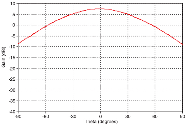
    The probe antenna was a small metal and ceramic chip, and we compared its performance with a small microstrip patch antenna mounted horizontally in a broader but otherwise similar housing, and a hexafilar antenna mounted in an identically dimensioned housing. Strictly, the microstrip antenna is a single terminal element, but it can be considered as self-resonant as the resonance fields are very tightly constrained. Figure 1 plots the radiation efficiencies for benign free-space conditions (without body-loading) together, as frequency responses.

    Source: GPS
    Figure 1. Frequency response of radiated efficiency in unloaded (free-space conditions) and mounted in similar housings (ground-plane width 55mm).

    In benign open-field conditions the probe antenna has excellent efficiency performance and superior bandwidth compared to the two self-resonant configurations. Conversely, the self-resonant antennas (patch and hexafilar) have similarly narrow frequency-response bandwidths and lower efficiencies. We will show how it is important to repeat the test for realistic use scenarios that determine how close the antenna will be juxtaposed to the user’s biological tissues before concluding that the probe antenna is the best solution.

    Antenna studies have shown that the bandwidth reduces very rapidly as the resonant volume of the antenna reduces. This accounts for the reduction in bandwidth shown in Figure 1 for the self-resonant antennas (microstrip patch and hexafilar) with respect to the probe antenna (chip). In the case of the probe, the resonant structure is the entire metal chassis of the device (in this case the circuit-board ground-plane) so that the resonant volume of the resonating system is much larger than those of the self-resonant structures.

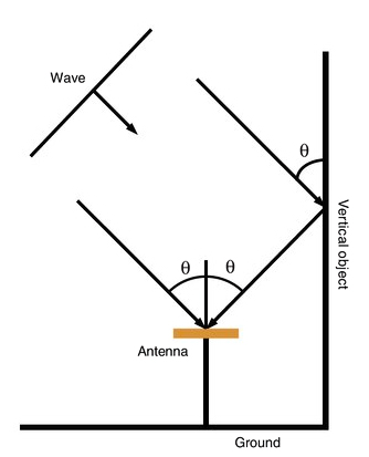
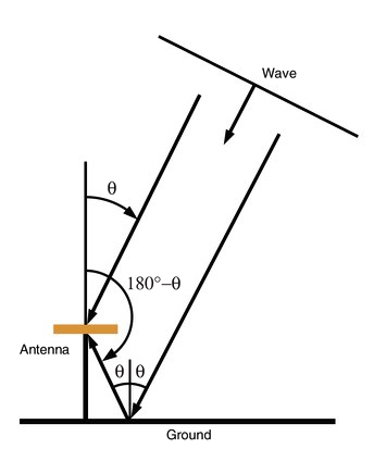
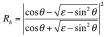
    To analyze the behavior of antennas in different use scenarios, it helps to consider the nature of resonance in antennas: open fields, with equal time average amounts of electric and magnetic field energy oscillating in space. These fields, induced by the time-varying voltage potentials and currents in the antenna, can launch a radiating wave into space because time-varying electromagnetic fields can carry or displace energy. We need to appreciate that this volume is where the so-called reactance fields exist, where field oscillations function as a sort of pump that propagates the electromagnetic wave. The antenna induces those fields in a configuration that manages the propagation of waves in useful directions and with desired polarization.

    Any invasion of the reactance field region will disrupt this process and cause impairment. Whilst obstruction of the radiating fields far away from the antenna will just cause a masking effect, a similar obstruction in the reactance-field region can disrupt the basic process of generating radiation. The density of fields in the reactance field region is much higher than would be implied by the straightforward application of the inverse square law.

    Use Near the Body

    We evaluated the antenna types, installed in packages as thin as test antenna dimensions allow, to draw conclusions as to how they might operate in slim-line consumer devices held close to the user’s body. Figure 2 shows CAD diagrams of the three antennas installed in their respective test packages.

    Source: GPS
    Figure 2. Antenna test housings for the chip antenna (left), patch antenna (middle) and hexafilar antenna (right). The housings were constructed to have a height of 26mm, a width of 60mm and a depth of 11 mm for the chip antenna and the hexafilar antenna and of 20.5mm for the patch antenna. In all cases the horizontal width extent of the printed circuit board (with continuous copper ground-plane on at least one side) was set at 55mm.

    Consumer devices have drawn antenna technologies from traditional GNSS applications as well as from terrestrial mobile telephone origins. The overall evolution combines adaptation of the circularly polarized technologies (multi-filar and microstrip patch) into smaller body-loaded platforms with insufficient space for effective ground-planes, together with adaptation of the art of low-cost cellular-telephone embedded antenna technologies that were never developed for circular polarization. Taking our three solutions in their embedded test platforms, we can appraise their body-loaded efficiencies by testing them juxtaposed to a phantom head, providing a means of assessing impairment due to body-loading.

    The phantom head in the loading experiment was filled with a tissue simulating liquid conforming to requirements for specific energy absorption measurements according to CENELEC and IEEE procedures. Comparing the antenna efficiencies for open-field conditions (Figure 1) and body-loaded conditions (Figure 3), reveals impairment to antenna efficiency in all three cases, with the most severe loss of approximately 80 percent by the chip antenna.

    Source: GPS
    Figure 3. Combination of FFT-based acquisition with FDAF.

    The self-resonant antennas suffered less impairment: approximately 30 percent reduction for the patch and 65 percent for the hexafilar antenna. The probe’s significant loss of efficiency is typical of this class of antennas, as the resonant fields are heavily loaded by the phantom head. The peak efficiency for this chip antenna has tuned downwards in frequency as the dielectric loading effect of the head-phantom introduced a regime of net higher relative dielectric constant (εr) into the resonance field region of the antenna system.

    By contrast, the self-resonant antennas did not tune down in frequency as they were brought into proximity with the phantom head. This indicates that the resonance fields were not offered to the dielectric materials of the head phantom to an extent that materially changed the relative dielectric constant (εr).

    Nevertheless, there is a significant difference between the impairment that develops between the patch and hexafilar cases as body-loading is applied, with the hexafilar solution losing more radiation efficiency than the patch antenna. There are two explanations for this difference.

    The first is that the patch housing is simply larger, with a greater depth required to accommodate the patch antenna horizontally at the top of the device housing. On average this larger housing size spaces the resonant fields further from the phantom and from the lossy simulated head tissues.

    The second explanation offers an insight into the symbiotic relationship between the hexafilar antenna and the demonstration platform’s vertically orientated housing. The horizontal ground-plane required for the patch antenna is inconvenient from the style and total integration cost point of view, but also ineffective as a ground-plane as it lacks sufficient width in a device styled to minimize depth. In this scenario the patch antenna is not getting much reflection uplift from the ground-plane; therefore there is little impairment when the device is body-loaded.

    The hexafilar solution is designed to benefit from reflective uplift from the vertically disposed ground-plane of the device. This property is convenient for device packaging because it allows the hexafilar antenna to be integrated at a device corner. The installation of a large and effective vertically oriented ground-plane for the hexafilar case is, by contrast, highly convenient and potentially more cost-effective. When the device is not body-loaded, reflections from the vertically disposed ground-plane uplift the gain and efficiency of the hexafilar antenna. The important advantage over the chip antenna (which is also convenient for space-constrained designs) is that for the self-resonant hexafilar antenna, the frequency of resonance does not change for open-field and body-loaded cases.

    Polarization, Pattern, Positioning

    Sufficient data has now been presented to make an antenna selection on the basis of efficiency and styling. The probe antenna in the guise of a chip antenna provided the highest radiation efficiency in free-space, comparable radiation efficiency to the hexafilar antenna in a body-loaded use scenario, and the small physical size supports compact product designs. However, for GNSS applications we must consider wave polarization, especially if there is multipath scattering. GNSS systems employ right-hand circular polarization (RHCP) and ideally should use antennas with hemisphereically omni-directional antennas. The zenith gain of a circularly polarized antenna is expected to be 3dB higher than that of a linearly polarized antenna of the same efficiency.

    If a GNSS terminal is equipped with an omni-directional but linearly polarized antenna, it can receive circularly polarized signals from all directions (albeit with a spatial average 3dB polarization loss). However, the positioning performance of such a terminal will be compromised because a linearly polarized antenna cannot discriminate between RHCP or LHCP, and reflections change the direction of spin of the circularly polarized wave.

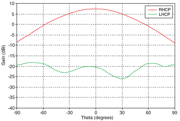
    More color to the subjects of polarization, pattern, and consequential GNSS accuracy can be gained by focussing on the operation of the dielectric-loaded hexafilar antenna, as an example of a small antenna. Figure 4 shows the measured RHCP and LHCP elevation patterns of an exemplary small hexafilar antenna. These are excellent examples of the signature cardiod pattern shapes of good circular polarization antennas, but they point in opposite boresight directions. A dipole rotating anti-clockwise (viewed from above) in a plane would simultaneously excite a RHCP cardiod elevation pattern in the upwards direction and an oppositely directed, but otherwise similar, LHCP cardiod pattern downwards. If the antenna has no ground-plane and the dipole rotation is planar, the power of the upward RHCP and downward LHCP responses are equal. However, the dielectrically-loaded hexafilar antenna is a synthesis of a small travelling-wave upwardly spiralling dipole, emulating the axial-mode of a helical antenna. As the electrical size of such an antenna is increased, the area of the upwardly directed RHCP pattern progressively increases, and the area of the downwardly directed LHCP pattern progressively reduces. The antenna’s dielectric core enables this right-to-left discrimination within dimensions that are very much smaller than a free-space wavelength of the GNSS signal.

    Source: GPS
    Figure 4. RHCP and LHCP elevation for small dielectrically loaded hexafilar antenna (with no ground-plane).

    We can describe the polarization sorting behavior of the small dielectrically loaded antenna in figure 4 as follows. GNSS signals direct from the space vehicles will arrive in the directions of the upper hemisphere of the patterns where the highest sensitivity of the antenna to RHCP is deployed. GNSS signals bounced from a reflective object may also arrive in these upper hemisphere directions, but with reversed polarization: LHCP. In these directions the antenna has a very much lower sensitivity to LHCP, and the GNSS receiving process will accord a low value on these signals that as a result of the low antenna gain will be assessed as relatively noisy.

    Signals that arrive at the antenna from directions in the lower hemisphere will certainly have reflected from the ground surface (assuming that the antenna is held upright). These reflected left-hand polarized signals may have been attenuated by absorption losses of materials present on ground surfaces and also reduced in GNSS receiver process weighting by the antenna’s discrimination in favor of RHCP.

    RHCP and LHCP Gain

    Whilst appraisal of antenna patterns is certainly the most important method for assessing the performance of antennas in different use scenarios, it is nevertheless difficult to report accurately because the three-dimensional data-set is inevitably complex. To provide a meaningful physical basis for discriminating performance between the test antennas for open-field and body-loaded, we propose a single parameter: cross-pole rejection at zenith as one which is directly relevant to GNSS accuracy in a multi-path environment. Figure 5 plots the right hand and left hand comparative frequency responses for open-field and body-loaded use scenarios. Table 1 summarizes these responses.

    (a)

    Source: GPS

    (b)

    (c)

    Source: GPS

    (d)

    Source: GPS
    Figure 5. RHCP and LHCP frequency responses at the zenith direction for conditions of free-space and body-loading. From top to bottom: a) open-field conditions and RHCP, b) open-field conditions and LHCP, c) body-loaded conditions and RHCP, and d) body-loaded conditions and LHCP.
    Source: GPS
    Table 1. RHCP to LHCP gain ratio at the zenith direction (θ=0, φ=0) at GPS L1 center frequency (1.575.42 GHz).

    In open field, the chip antenna does not have a gain advantage for right-hand versus left-hand polarization and also suffers the highest impairment in gain when body-loading is applied. In this test there is an advantage in favor of RHCP gain for the body-loaded test scenario, but we presume this depends on the mounting position of this particular probe antenna on the test device. Perhaps a mounting position towards the left of the assembly might have incurred a disadvantage of similar magnitude?

    The patch antenna has an excellent RHCP over LHCP advantage in open-field conditions, but this advantage diminishes when this solution is body-loaded. This is the least gain-impacted solution as presumably the horizontal ground-plane and much greater device width produce a relatively low body-loading impact.

    The most interesting result concerns the hexafilar antenna, for which the RHCP to LHCP advantage actually improved in the body-loaded test scenario. As this device had the same depth, one might have expected it to sustain a body-loading impairment similar to that of the chip antenna, but due to the self-resonant character of the hexafilar element the loss in gain (in this zenith direction) was actually only slightly greater than that of the patch antenna.

    The hexafilar element’s CP performance is distorted by the lack of circular symmetry of the vertical ground-plane; therefore in open field this direction has a relatively modest RHCP to LHCP gain advantage of about 5dB. However, when the device containing the hexafilar antenna solution is body-loaded, the re-radiation from reflections from the circuit-board are heavily damped by the phantom head. The radiating source is then predominantly the hexafilar self-resonant element that by design is not itself so significantly impacted by the body-loading scenario. This source is restored to a more autonomous circularly polarized form with an advantage of RHC versus LHCP gain in zenith direction, nearly 13.5dB.

    Walk Tests

    Free-space and body-loaded test data, together with arguments concerning polarization discrimination and multipath led to an hypothesis that the antennas with the best circular polarization performance should provide the highest GNSS positioning accuracy. We tested the three devices, worn against the lower torso where the body provides a relatively homogeneous dielectric medium, so that position data could be compared with a reference antenna mounted over a large overhead ground plane.

    Many walk tests were conducted around different routes in London, which collectively demonstrate the value of circular-polarization discrimination as a key enabler for accurate street-level position determination. One segment (Figure 6) in the vicinity of an iconic tall London building commonly known as the Gherkin showed that, though the circularly polarized antennas closely followed the path of the reference antenna, the linearly polarized chip antenna produced an error of as much as 200 meters. It is possible that the dominant reflector in this case is the Gherkin itself.

    Source: GPS
    Figure 6. Data, central London walk test.

    Conclusions

    The chip and hexafilar antennas could be integrated tightly into consumer device housings; both experienced gain uplift from the vertically disposed circuit-board ground-plane. The gain uplift from the chip antenna arose as the resonant volume of the device is enlarged as the device size is increased. The gain uplift from the hexafilar antenna arose as a result of constructive reflections from the circuit-board functioning as a vertical ground-plane.

    The patch antenna was not the most convenient from the styling point of view because the depth was dictated by the size of the horizontally orientated patch. Consequently the housing was significantly thicker than for the chip and hexafilar solutions, and the patch antenna was not receiving significant uplift from reflections from the housing because the depth limitation constrained the ground-plane to ineffective dimensions.

    In body-loaded tests, the chip and hexafilar antennas demonstrated roughly equal radiation efficiency, but the hexafilar provided a significant RHCP advantage. Higher right-hand circular gain was measured for the patch antenna; this was expected due to the greater depth of the housing to accommodate the patch antenna. Urban walk tests showed that the RHCP antennas provided the highest position accuracy.

    Whilst the hexafilar antenna did experience some uplift due to reflections from the device circuit board, these were negated when the device was body-loaded. However, the distorting effects of the device ground-plane were also lost, so that the antenna’s advantage of RHCP over LHCP was improved in the body-loading condition.

    The GNSS industry has advanced the miniaturization of polarization-controlled antennas for small body-loaded uses. This is gaining currency as enabling polarization diversity in 4G data-communication terminals.

    Manufacturers

    Sarantel SL1350 antenna was the hexafilar element under test.

    Position data for all four devices was measured with Telit SE868 evaluation kits using CSR (now Samsung) SiRFstarIV chipset.


    Oliver Leisten is chief technical officer and founder of Sarantel Limited, where Viktor Knobe worked as a student intern from Imperial College London.


  • Tallysman Wireless Introduces Wideband, Low Cost GPS-L1/GLONASS Antenna

    Tallysman Wireless, Inc., has announced the latest addition of the TW4320/4322 to its line of antenna products. The TW4320/TW4322 antennas are small wide-band, high-performance antennas housed in a compact IP67 magnetic mount enclosure, with a three-meter cable and a wide range of connectors.
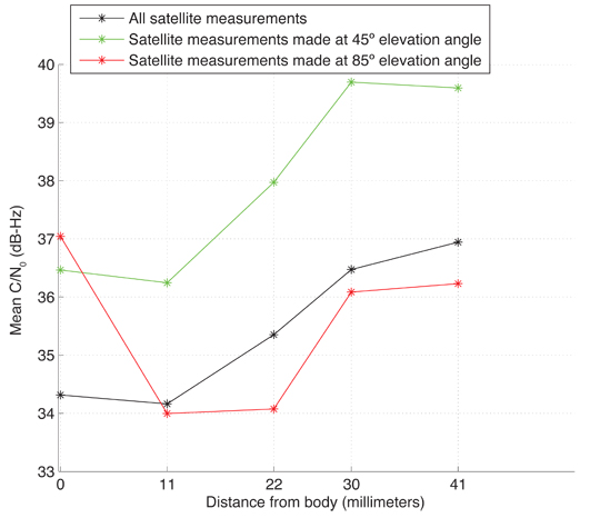
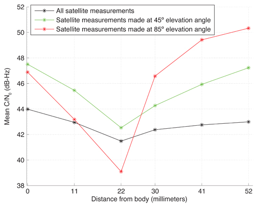
    “Most small low-cost GPS and GLONASS antenna have narrow-band patch elements tuned mid-way, but which are 2-dB down in both signal bands,” said Gyles Panther, CEO of Tallysman Wireless. “The TW4320/22 antennas feature a patch element with a 40% wider bandwidth and a very low noise amplifier which together allows the full benefits of multi-constellational GNSS to be realized.”

    The TW4320/TW4322 antenna covers the GPS L1, GLONASS L1, and SBAS (WAAS, EGNOS, and MSAS) frequency bands (1575 to 1606 MHz). It features a small patch element with 40 percent wider bandwidth than previously available in this format. It provides both GPS-L1 and GLONASS signals in the 1-dB received power bandwidth.

    The TW4320/TW4322 has a two stage low-noise amplifier with a mid-section SAW (Surface Acoustic Wave). A tight pre-filter is available in the TW4322 to protect against saturation by high-level sub-harmonics and L-band signals.

    Features:
    •    
40% wider bandwidth in the same format
    •    Axial ratio: 6 dB max
    •    Low noise LNA: 1 dB
    •    High rejection mid-section SAW filter
    •    Available pre-filter (TW4322)
    •    High gain: 28 dB typ.
    •    Wide voltage input range: 2.5 to 10 VDC
    •    IP67 weather-proof housing
    Models:
    •   TW4320 – GPS/GLONASS antenna, three-meter cable, SMA Male 32-4320-xx-yyyy
    •   TW4322 – GPS/GLONASS antenna, with pre-filter, three-meter cable, SMA Male 32-4322-xx-yyyy

  • GLONASS Antenna

    Taoglas is launching the AA.16X Dominator series of antennas, which have a wider bandwidth to cover the GLONASS operating frequencies up to 1610 MHz, a good axial ratio, and a double resonance design for optimum reception at the center frequencies.

    Taoglas’ GPS antennas are being used in the field by many different M2M solution providers including tracking, telematics, and GPS manufacturers, the company said.

    The AA.161 Dominator is a magnetic mount GPS-GLONASS IP67, external antenna incorporating a 35-millimeter ceramic patch. It is a wide-band active patch antenna product with a large integral ground that delivers a gain up to 35 dB. With the Dominator antenna series, Taoglas has a comprehensive range of GPS-GLONASS active embedded antennas (AGGP series) and passive embedded (CGGP) antennas for automotive first-tier TS16949 and after-market applications.

    “In the coming months, for the first time the true availability of GPS and GLONASS satellites along with the latest generation of GNSS receivers are going to dramatically change the performance of M2M location devices,” said Ronan Quinlan, Director Taoglas. “With close to double the amount of satellites to draw from compared to a stand-alone GPS constellation, we are now going to see quicker time to first fixes with accuracy improving from meters to sub one meter. The ability to view and lock on four or more satellites in traditionally difficult reception areas such as urban canyons, city centers or locations with restricted views of the horizon, will give M2M manufacturers the ability to triangulate and pinpoint locations with greater accuracy and with quicker time to first fix.

    Taoglas’ new Dominator antennas have been rigorously tested and pre-approved by the GNNS receiver companies worldwide and have been shown to display higher and more consistent gain in comparison to competing antennas, the company claimed. Two key components have been engineered from scratch for the Dominator series, a wide-band front-end SAW filter (critical to prevent out of band noise entering on both GPS and GLONASS degrading the signal) and a high-gain 35-mm patch.

    CONTACT INFO

    Company: Taoglas
    Country: United States (USA)
    URL: http://www.taoglas.com

  • Taoglas Offers Dominator Antenna with Wider GLONASS Bandwith

    Taoglas Offers Dominator Antenna with Wider GLONASS Bandwith


    Photo: Taoglas

    Taoglas is launching the AA.16X Dominator series of antennas, which have a wider bandwidth to cover the GLONASS operating frequencies up to 1610 MHz, a good axial ratio, and a double resonance design for optimum reception at the centre frequencies. The company will showcase its line of antennas at CTIA in New Orleans May 8-10.

    Taoglas’ GPS antennas are being used in the field by many different M2M solution providers including tracking, telematics, and GPS manufacturers, the company said.

    The AA.161 Dominator is a magnetic mount GPS-GLONASS IP67, external antenna incorporating a 35-millimeter ceramic patch. It is a wide-band active patch antenna product with a large integral ground that delivers a gain up to 35 dB. With the Dominator antenna series, Taoglas has a comprehensive range of GPS-GLONASS active embedded antennas (AGGP series) and passive embedded (CGGP) antennas for automotive first-tier TS16949 and after-market applications.

    “In the coming months, for the first time the true availability of GPS and GLONASS satellites along with the latest generation of GNSS receivers are going to dramatically change the performance of M2M location devices,” said Ronan Quinlan, Director Taoglas. “With close to double the amount of satellites to draw from compared to a stand-alone GPS constellation, we are now going to see quicker time to first fixes with accuracy improving from meters to sub one meter. The ability to view and lock on four or more satellites in traditionally difficult reception areas such as urban canyons, city centers or locations with restricted views of the horizon, will give M2M manufacturers the ability to triangulate and pinpoint locations with greater accuracy and with quicker time to first fix.”

    Taoglas’ new Dominator antennas have been rigorously tested and pre-approved by the GNNS receiver companies worldwide and have been shown to display higher and more consistent gain in comparison to competing antennas, the company claimed. Two key components have been engineered from scratch for the Dominator series, a wide-band front-end SAW filter (critical to prevent out of band noise entering on both GPS and GLONASS degrading the signal) and a high-gain 35-mm patch.

  • Innovation: GNSS Antennas and Humans

    Innovation: GNSS Antennas and Humans

    A Study of Their Interactions

    By Jared B. Bancroft, Valérie Renaudin, Aiden Morrison, and Gérard Lachapelle

    GPS World photo
    INNOVATION INSIGHTS by Richard Langley

    GPS IS VIRTUALLY UBIQUITOUS with more than 400 million units estimated to be in use in the United States alone. Some of these units are standalone devices such as those used in surveying and timing applications and those used for vehicle navigation or tracking with permanent or temporary mountings. However, the majority of the units are integrated into cellular telephones, tablet computers, personal digital assistants, watches, cameras, and other devices, which are designed to be operated in close contact with the human body. We even now have GPS shoes!

    It is well known that the performance of the antenna of a radio receiver can be affected when it is used in close proximity to the human body. We only have to touch the whip antenna of a portable AM/FM or scanner radio to convince ourselves of the effect. So, when we use a handheld GPS receiver or wear a GPS watch, or put a GPS-equipped cellular telephone up to our ear, are there any effects on the operation of the receiver?

    It turns out that there are four major effects that can change the performance of a GPS (or other GNSS) receiver antenna when placed near or on the human body. The impedance of the antenna may be changed causing a drop in power transfer to the receiver front end. The center frequency and bandwidth of the antenna may be changed again resulting in a loss of received power. The gain pattern of the antenna may be changed. However, the change may be favorable, improving reception for a given satellite azimuth and elevation angle. And lastly, there will be close-range multipath between the antenna and the body skin.

    All of these factors need to be taken into consideration when a manufacturer is designing a GPS unit to be operated in close proximity to a human body. Trade-offs might be possible and certain designs may make the antenna less likely to interact with its surroundings.

    But how does one go about assessing the antenna’s performance in a repeatable and quantifiable way?

    In this month’s column, a team of researchers from The University of Calgary report on tests conducted on two different types of GPS antennas operated in the vicinity of a human phantom — an artificial body with similar electromagnetic properties as that of a real human.


    “Innovation” features discussions about advances in GPS technology, its applications, and the fundamentals of GPS positioning. The column is coordinated by Richard Langley, Department of Geodesy and Geomatics Engineering, University of New Brunswick. To contact him with topic ideas, email him at lang @ unb.ca.


    GNSS-based navigation is the foundation of many pedestrian navigation systems. The use and benefit of GNSS receivers to locate people has increased dramatically over the past few years. Pedestrian navigation applications include mobile phone users, first responders, health and activity monitoring, consensual tracking (such as offender management), recreational use, and tracking of military personnel. GNSS navigation systems are commonly available in watches and personal entertainment devices. Some applications contain GNSS receivers and antennas in shoes, glasses, and jackets. Since each application using a GNSS receiver to locate people requires an antenna, the optimal type, size, and location on the body is becoming increasingly important.

    This article addresses adverse antenna effects when the antenna is placed near or on the human body, specifically in the reactive near field at the GPS L1 frequency. Using real data collected on a human phantom over prolonged periods, the changes within the antenna are observed as a function of distance from the body. Thus, a performance profile can be generated to quantify the power loss incurred by loading the antenna. The study applies equally well to all GNSS operating at or near the GPS L1 frequency.

    The researchers have theoretically addressed performance of GPS antennas in close proximity to a human body. Using simulations to provide analysis of antenna detuning effects, one research group showed a 24.4-MHz shift in the resonance frequency of the antenna when placed 10–40 millimeters from a simulated human chest. The resonance shift was common at all distances, although the return loss decreased as the antenna was moved further away from the chest.

    A few studies have developed antennas to be located in protective (or otherwise) garments for specific applications. Our team previously analyzed the impact of antenna location on the human body by comparing the solution of eight identical and simultaneous navigation solutions.

    Antenna-Body Interaction

    Antenna detuning refers to the consequence of the electrical interaction between an antenna and an adjacent object, the body of a user in this context, which causes the center frequency of the antenna to deviate from the desired center frequency. More generally, there are several effects that serve to degrade antenna performance that arise when an antenna operates near the body of a user.

    The first of these effects is a change in the impedance of the antenna, as shown in FIGURE 1. (See online sidebar for antenna and electromagnetic radiation term definitions.) The change results in the impedance of the antenna no longer properly matching that of the network that it is expected to drive, therefore causing incomplete power transfer between the antenna element and the subsequent radio-frequency (RF) stages.


    Selected Antenna and Electromagnetic Radiation Terms

    Axial ratio. A measure of the polarization ellipticity of an antenna designed to receive circularly polarized signals. An axial ratio of unity, or 0 dB, implies a perfectly circularly polarized antenna.

    Bandwidth. The range of frequencies over which an antenna is designed to operate efficiently. The bandwidth limits are typically determined by a particular reduction in gain compared to that at the antenna’s center frequency; for example, 3 dB or 10 dB.

    Conductivity. A measure of a material’s ability to conduct an electric current. The reciprocal of resistivity. Units are mhos per meter.

    Dielectric. A material in which there are no free charges that can move through it under the influence of an electric field. An insulator. However, minute displacements of positive and negative charges in opposite directions are possible. A dielectric in which this charge displacement has taken place is said to be polarized.

    Far field. The area sufficiently far from an antenna where the gain pattern is essentially independent of distance. In the far field, the power of an electromagnetic wave traveling in free space drops off as the square of the distance from the transmitting antenna.

    Fresnel reflection coefficient. A measure of the degree of reflection of an electromagnetic wave at the interface between two media. Dependent on the properties of the media, the polarization of the wave, and the angle of incidence.

    Gain. For a transmitting antenna, the ratio of the radiation intensity in a given direction to the radiation that would be obtained if the power accepted by the antenna was radiated isotropically. For a receiving antenna, it is the ratio of the power delivered by the antenna in response to a signal arriving from a given direction compared to that delivered by a hypothetical isotropic reference antenna.

    Gain (amplitude) pattern. The spatial variation of an antenna’s gain.

    Human phantoms. Models of parts of the human body used in engineering, science, and medical studies designed to mimic a particular physical, chemical, or electrical behavior.

    Impedance. The complex ratio of the voltage to the current in an alternating current circuit. Sometimes called complex resistance in which case the absolute value of the complex resistance is called the impedance. Units are ohms.

    Lossy material. A material in which a significant amount of the energy of a propagating electromagnetic wave is absorbed (dissipated) per unit distance traveled by the wave.

    Near field. The region around an antenna within a few wavelengths where there are strong inductive and capacitive effects from the currents and charges in an antenna that cause electromagnetic components not to behave like far-field radiation. Within the radiating part of the near field, the gain pattern is dependent on the distance from the antenna.

    Polarization. The sense of vibration of electromagnetic radiation. There are two main types of polarization: linear, in which the radiating wave’s electric field vector is confined to a particular direction (typically vertical or horizontal); and circular, where the electric field vector rotates as the wave propagates through space. Depending on the sense of rotation, a signal’s waves may be left-hand or, as with GPS signals, right-hand circularly polarized. For maximum response, the polarization of a receiving antenna should match the polarization of the signals.

    (Absolute) Permittivity. A measure of how an electric field affects, and is affected by, a dielectric material. In a sense, it describes a material’s ability to transmit (or “permit”) an electric field. Since the response of most materials to external fields generally depends on the frequency of the field, permittivity is expressed as a complex quantity with real and imaginary components as a function of frequency. Units are farads per meter.

    Relative permittivity. The ratio of the permittivity of a material to that of free space or a vacuum. Also called the dielectric constant. Unitless.

    Return loss. A measure of the effectiveness of power delivery from a transmission line to a load such as an antenna or vice versa. If the power incident on an antenna is Pin and the power reflected back to the source is Pref, the degree of mismatch between the incident and reflected power in the traveling waves is given by the ratio  Pin/Pref.  Units are dB. Functionally related to the Fresnel reflection coefficients and VSWR.

    Voltage standing wave ratio (VSWR). A measure of the size of the reflected waves in a transmission line due to impedance mismatches between the line and a connected antenna. The ratio of the maximum voltage along the line to the minimum voltage along the line. Ideally, an antenna should have a VSWR value of unity.


     FIGURE 1. Change in the reactive portion of the impedance of a patch antenna versus separation distance between the antenna element and imitation human skin (Courtesy, Buckley et al., 2010; see Further Reading). Credit: Jared B. Bancroft, Valérie Renaudin, Aiden Morrison, and Gérard Lachapelle and Richard Langley
    FIGURE 1. Change in the reactive portion of the impedance of a patch antenna versus separation distance between the antenna element and imitation human skin (Courtesy, Buckley et al., 2010; see Further Reading).

    The figure provides an example of the impedance for a patch antenna plotted against the separation distance of a simulated human wrist. When mounted directly on the user’s skin surface, this specific antenna gains significant reactive impedance that results in a large voltage standing wave ratio (VSWR) with the network.

    A second effect of antenna proximity to human skin is the alteration of the center frequency, as well as the alteration of the antenna bandwidth. Depending on the bandwidth of the signal of interest, the bandwidth of the antenna element, and the degree of center-frequency shifting and bandwidth loss experienced, these factors can contribute to significant loss of received power.

    Thirdly, it is important to note that in some configurations, a “lossy” medium adjacent to an antenna may improve the apparent performance of the antenna due to changes in its gain pattern that result in better receive or transmit performance for a given azimuth and elevation angle.

    For any application in which the antenna may be either in free space or directly adjacent to a lossy medium such as a human body, the use of balanced antennas is recommended. The image current of a balanced antenna is contained within complementary structures of the antenna itself, not within the casing or adjacent material of the antenna, therefore making the antenna much less likely to interact with surrounding media.

    Fourth, the close proximity of a reflective material increases close-range multipath. If the distance between the reflector (that is, skin) and the antenna is close to half a wavelength, giving a 180º phase shift of the carrier, deconstructive interference can occur. There are several factors that contribute to this including the back lobe of the antenna gain pattern, reflection coefficient of the skin beneath the antenna, and the incident angle of the incoming ray. Approximation via simple ray tracing becomes dauntingly complex due to the variation of the antenna properties listed above, resulting from detuning. Therefore, observation of the effect becomes easier than modeling an incoming ray and its multipath counterparts.

    Phantom Body Simulation

    To conduct an assessment of the impact of the human body on the radiation patterns of diverse antennas in the context of tracking GNSS signals, a human body phantom has been designed for collecting the experimental data. Variations of the locations and orientations of the antenna rigidly mounted on a human shoulder, head, or any other locations would render the repeatability and comparison of the collected data hardly feasible. Furthermore, the distance that separates the antenna from the human body surface could only be precisely controlled using an artificial modeling of the human body. Therefore, a human body phantom is required for productive analysis.

    Because the human body is mainly composed of water, the presence of human tissue in the vicinity of the antenna introduces an absorption and reflective effect that alters the performance of the antenna. Different mathematical models have been developed for representing the different component combinations of a human body. Based on the study of numerous women and men of different ages and sizes, a classic model predicting the fat-free mass of a person has been developed and assumes that 73 percent of a human body consists of water. Looking at the elemental composition in the human body, it can be found that a concentration of 7 grams of salt per liter of water provides an acceptable modeling of the human tissues. Complex shapes of the human body are used for modeling more precisely the layered structure of the human tissues using either a more realistic human phantom or a more detailed model comprising the extensive data on the dielectric properties of each layer constituting the human tissues of interest. For context of this study, the phantom was kept simple and was made of a large plastic container filled with a 7 percent concentration of a saline solution.

    The radiative transfer of the human body phantom on the reception of GNSS signals can be evaluated through the understanding of the dielectric permittivity of the solution. Different models, including the Wagner, Debye, Cole & Cole, or Fricke, are commonly used for studying the dielectric behavior of biological tissues. The Debye model gives the permittivity of an aqueous saline solution of salinity, S, at a fixed temperature, t, as

    Inn-Eq1 .Jared B. Bancroft, Valérie Renaudin, Aiden Morrison, and Gérard Lachapelle (1)

    where

    Screen shot 2013-01-04 at 10.01.10 PM . Jared B. Bancroft, Valérie Renaudin, Aiden Morrison, and Gérard Lachapelle is the angular frequency (Hz),

    εi equals 8.8419 ×10⁻¹² (farads per meter),

    τ is the relaxation time (seconds),

    σ is the ionic conductivity of the dissolved salts (mhos per meter), and

    ε0 and ε∞ are the static and high frequency dielectric constants.

    Equation (1) gives the dielectric proprieties of the human phantom solution for a specific temperature, saline concentration, and temperature. The experiments we conducted and report on in this article lasted several days and were conducted outside, which unfortunately resulted in temperature fluctuations. Consequently, the 7 percent saline solution over the temperature range of 11º to 31º C for L1 (1575.42 MHz) results in a 9 percent variation of permittivity. As shown in FIGURE 2, the dielectric constant over the experimental temperature range is in the interval [74.6, 81.9]. Because the variation is small, the permittivity value can be closely approximated to a mean value of 78.

     FIGURE 2. Real part of the permittivity of the human body phantom as a function of temperature for the GPS L1 frequency. Jared B. Bancroft, Valérie Renaudin, Aiden Morrison, and Gérard Lachapelle
    FIGURE 2. Real part of the permittivity of the human body phantom as a function of temperature for the GPS L1 frequency.

    Reflection Coefficient of the Phantom Body

    The Fresnel reflection coefficients for a smooth flat surface depend on frequency, the incident angle, polarization, and ground characteristics. Since the container is full of salted water it can also be considered a reflective surface.

    The relative permittivity of the saline solution given in Equation (1) can be reformatted as

    Inn-Eq2 . Jared B. Bancroft, Valérie Renaudin, Aiden Morrison, and Gérard Lachapelle (2)

    The reflection coefficients with vertical and horizontal polarizations, respectively, of the electromagnetic wave on the surface of the saline water are given by the following Fresnel equations:

    Inn-Eq3 . Jared B. Bancroft, Valérie Renaudin, Aiden Morrison, and Gérard Lachapelle(3)

    Inn-Eq4 . Jared B. Bancroft, Valérie Renaudin, Aiden Morrison, and Gérard Lachapelle(4)

    where Rv and Rh are the vertical and horizontal polarized reflection coefficients, respectively, and θ is the incident angle.

    Assuming that the water surface is flat and infinite, Equations (3) and (4) are plotted against the incident angle in FIGURE 3. The reflection coefficients were estimated using a mean temperature of 21°C, a salt concentration of 7 percent and at the L1 frequency.

     FIGURE 3. Fresnel coefficient for L1 considering a flat surface of salted water. Jared B. Bancroft, Valérie Renaudin, Aiden Morrison, and Gérard Lachapelle
    FIGURE 3. Fresnel coefficient for L1 considering a flat surface of salted water.

    While the saline solution of the human phantom has an angle of incidence and direction of polarization dependent on reflectivity, the fact that the GPS carrier is circularly polarized must be considered. Due to the circular polarization of the carrier and that of most antenna elements intended for GPS use, the received signal strength of the reflected wave will always appear to be equal to or higher than that of the reflected portion of the horizontal polarization.

    Test Setup

    To evaluate the change in gain pattern as function of distance from the phantom, we collected 24-hour data segments. These segments allowed the receiver to observe all satellites. A high-performance GPS L1 receiver module evaluation kit was used with two antennas. The first was a patch antenna while the second was a quadrifilar helix antenna. FIGURE 4 shows both antennas without their coverings. Each antenna has a built-in low noise amplifier (LNA). The antenna specifications are listed in TABLE 1.

     FIGURE 4. Patch (above) and quadrifilar (below) antennas used in the tests. Jared B. Bancroft, Valérie Renaudin, Aiden Morrison, and Gérard Lachapelle
    FIGURE 4. Patch (above) and quadrifilar (below) antennas used in the tests.
     TABLE 1. Antenna specifications. Jared B. Bancroft, Valérie Renaudin, Aiden Morrison, and Gérard Lachapelle
    TABLE 1. Antenna specifications.

    A water container holding the saline solution was placed on the roof of a building as shown in FIGURE 5. The container had a slight inclination to move a small air pocket to the corner of the container away from the antenna. After a successful 24-hour data collection period, the antenna was supported by a small plastic box and oriented in the same direction. Six vertical distances were selected, namely 0, 11, 22, 30, 41, and 52 millimeters.

     FIGURE 5. Data collection with patch antenna fixed to phantom body. Jared B. Bancroft, Valérie Renaudin, Aiden Morrison, and Gérard Lachapelle
    FIGURE 5. Data collection with patch antenna fixed to phantom body.

    The gain pattern as measured by the C/N0 values of the path antenna is shown in FIGURE 6. In general, the largest effect is seen near the zenith where the power decreased by 10–15 dB when the antenna was 22 millimeters from the phantom body. It is also observed that the effect is maximized at 22 millimeters, and then reverts back to near normal operation at 52 millimeters. Additionally, at lower elevation angles (< 30º), the gain behaves more linearly, where the largest distance has the least gain, while the smallest distance has the most gain. The effect of the phantom body appears to flatten the gain pattern.

    The pattern shown in Figure 6 shows the effect of the proximity to the phantom body over all elevation angles. However, a prominent pattern emerges for measurements made at elevation angles of 45º and 85º. In the case of a 22-millimeter antenna distance from the body, a significant power decrease occurs. For satellites with an 85º elevation angle, nearly 8 dB is lost compared to 5 dB loss at a 45º elevation angle.

     FIGURE 6. Gain pattern of the patch antenna as measured by the measured C/N0 at all elevation angles as a function of antenna distance from body. Elevation angles [0º, 90º] have azimuths [180º, 360º], while elevation angles [90º, 180º] have azimuths [0º, 180º]. Jared B. Bancroft, Valérie Renaudin, Aiden Morrison, and Gérard Lachapelle
    FIGURE 6. Gain pattern of the patch antenna as measured by the measured C/N0 at all elevation angles as a function of antenna distance from body. Elevation angles [0º, 90º] have azimuths [180º, 360º], while elevation angles [90º, 180º] have azimuths [0º, 180º].
    FIGURE 7 provides the trend as a function of distance from the body. The trend of the power loss at 22 millimeters is common on all measurements, albeit more significant for higher-elevation-angle satellites. For satellite measurements made at an 85º elevation angle, the power varies by 12 dB. When all measurements are considered, which includes more frequent lower-elevation-angle satellite measurements and the fact that the gain pattern deviates significantly at higher elevation angles (as shown in Figure 6), the fluctuation is less prominent.

     FIGURE 7. Mean C/N0 measurements of the patch antenna from all measurements and those only at 45º and 85º elevation angles as a function of antenna distance from the body. Jared B. Bancroft, Valérie Renaudin, Aiden Morrison, and Gérard Lachapelle
    FIGURE 7. Mean C/N0 measurements of the patch antenna from all measurements and those only at 45º and 85º elevation angles as a function of antenna distance from the body.

    To assess the cause of the impact, we removed the phantom and replaced it with a flat aluminum reflector placed beneath the antenna. The antenna was then placed at the same distances above the reflector as previously. Since the gain pattern had been established and this test was to observe the effect of the reflector, only 60 seconds of data was collected at each distance.

    FIGURE 8 provides the change in C/N0 for two tests, which has a comparable trend to that of Figure 7. From the corroboration of the two tests, it appears that the salt water provides similar multipath effects to that of the aluminum sheet. The power loss is then attributed to destructive interference.

     FIGURE 8. Mean C/N0 measurements (over 60 seconds) of satellite PRN 8 with 85º elevation angle when placed above an aluminum reflector. Jared B. Bancroft, Valérie Renaudin, Aiden Morrison, and Gérard Lachapelle
    FIGURE 8. Mean C/N0 measurements (over 60 seconds) of satellite PRN 8 with 85º elevation angle when placed above an aluminum reflector.

    Similar data collections were conducted with the quadrifilar helix in order to assess its ability to perform close to the human phantom. The quadrifilar antenna has the LNA circuitry vertically below the antenna and therefore was placed horizontally on the water container. FIGURE 9 shows its gain pattern. The overall C/N0 is lower but is subject to less variation compared to that of the patch antenna. In general, we noticed lower C/N0 values with the quadrifilar antenna, regardless of the environment and despite the LNA having 5 dB more amplification. Some moderate variations of up to 10 dB appear on the east side of the antenna (zenith angle [0º, 90º]), but overall the pattern appears to be more regular.

     FIGURE 9. Gain pattern of the quadrifilar antenna as measured by the C/N0 of all measurements as a function of antenna distance from body. Elevation angles [0º, 90º] have azimuths [180º, 360º], while elevation angles [90º, 180º] have azimuths [0º, 180º]. Jared B. Bancroft, Valérie Renaudin, Aiden Morrison, and Gérard Lachapelle
    FIGURE 9. Gain pattern of the quadrifilar antenna as measured by the C/N0 of all measurements as a function of antenna distance from body. Elevation angles [0º, 90º] have azimuths [180º, 360º], while elevation angles [90º, 180º] have azimuths [0º, 180º].
    The overall power variation was assessed in a similar method. FIGURE 10 shows cubic-like functions with 3-dB variations. There is also no consistent downward power loss trend at 22 millimeters as observed with the patch antenna. As expected, due to the balanced nature of the quadrifilar antenna, the degree of apparent power loss caused by adjacent material is substantially lower compared to the patch antenna. While the peak level of power received is not as high as that experienced with the patch antenna, the consistency of the received power level is better.

     FIGURE 10. Mean C/N0 measurements of the quadrifilar antenna from all measurements and those only at 45º and 85º elevation angles as a function of antenna distance from the body. Jared B. Bancroft, Valérie Renaudin, Aiden Morrison, and Gérard Lachapelle
    FIGURE 10. Mean C/N0 measurements of the quadrifilar antenna from all measurements and those only at 45º and 85º elevation angles as a function of antenna distance from the body.

    Conclusions

    We have investigated the impact of the proximity of the human body on received signal power associated with operation of L1 GPS antennas through experimental tests. GPS signals have been collected using two different antenna types (a patch antenna and a quadrifilar helix antenna), placed on a human body phantom with different separation distances. A strong relationship between these distances and the averaged received signal power has been observed for both antennas with overall lower C/N0 values for the quadrifilar antenna. The largest attenuation is not observed when the antenna is directly adjacent to the user body but when it is about 22 millimeters above it. We found that the attenuation mainly results from destructive interference due to multipath. These results suggest that body-mounted GPS antennas should be directly in contact with the user’s body for achieving better tracking performance. Our future research will include theoretically assessing the experimental results for better understanding of the underlying effects.

    Acknowledgments

    This article is based on the paper “GNSS Antenna-Human Body Interaction” presented at ION GNSS 2011, the 24th International Technical Meeting of the Satellite Division of The Institute of Navigation, Portland, Oregon, September 19–23, 2011. The authors would like to thank Prof. Ron Johnston, Dept. of Electrical and Computer Engineering, The University of Calgary, for his insight and consultation in preparing that paper. We thank John Buckley, Tyndall National Institute, Ireland, and his co-authors for permission to use Figure 1, a version of which appears in “The Detuning Effects of a Wrist-Worn Antenna and Design of a Custom Antenna Measurement System” (see Further Reading).

    Manufacturers

    The tests discussed in this article used a u-blox AG EVK-6T evaluation kit using a LEA-6T L1 GPS module, an Allis Communication Co. Ltd. M827B active L1 patch antenna, and a Sarantel Ltd. SL1206 active L1 quadrifilar helix antenna.


    Jared B. Bancroft is a senior research engineer in the Position, Location And Navigation (PLAN) Group in the Department of Geomatics Engineering at The University of Calgary in Calgary, Alberta, Canada. He received his Ph.D. in geomatics engineering in 2010 and has worked in the area of navigation since 2004. Dr. Bancroft’s research interests include pedestrian and vehicular navigation through data fusion of sensors and satellite navigation data.

    Valérie Renaudin is a senior research associate in the PLAN Group. She received an M.S. in geomatics engineering from the Ecole Supérieure des Géomètres et Topographes, France, in 1999 and a doctorate in geomatics engineering from the Ecole Polytechnique Fédérale de Lausanne, in 2009. She was previously the technical director at Swissat AG. Her research interests include low-cost sensors, hybridization techniques, magnetometers, and indoor navigation.

    Aiden Morrison is a senior research associate in the PLAN Group. He received his B.Eng. in electrical engineering from Ryerson University, Canada, in 2006 and a Ph.D. in geomatics engineering from The University of Calgary in 2010. His research interests include development of integrated navigation systems.

    Gérard Lachapelle holds a Canada Research Chair in Wireless Location in the Department of Geomatics Engineering at The University of Calgary, where he has been a professor since 1988 and heads the PLAN Group. He has been involved in a multitude of GNSS R&D projects since 1980, ranging from RTK positioning to indoor location and GNSS signal processing enhancements.


    Further Reading

    • Previous Work by Authors
    “GPS Observability and Availability for Various Antenna Locations on the Human Body” by J.B. Bancroft, G. Lachapelle, T. Williams, and J. Garrett in Proceedings of ION GNSS 2010, the 23rd International Technical Meeting of the Satellite Division of The Institute of Navigation, Portland, Oregon, September 21–24, 2010, pp. 2941–2951.

    • GNSS Antennas
    Mobile-Phone GPS Antennas: Can They be Better?” by T. Haddrell, M. Phocas, and N. Ricquier in GPS World, Vol. 21, No. 2, February 2010, pp. 29–35.

    GNSS Antennas: An Introduction to Bandwidth, Gain Pattern, Polarization, and All That” by G.J.K. Moernaut and D. Orban in GPS World, Vol. 20, No. 2, February 2009, pp. 42–48.

    A Primer on GPS Antennas” by R.B. Langley in GPS World, Vol. 9, No. 7, July 1998, pp. 73–77.

    • Interaction between Receiving Antennas and Human Body Parts
    “The Detuning Effects of a Wrist-Worn Antenna and Design of a Custom Antenna Measurement System” by J. Buckley, K.G. McCarthy, B. O’Flynn, and C. O’Mathuna in Proceedings of the 40th European Microwave Conference, Paris, France, 28–30 September 2010, pp. 1738-1741.

    “One-Layer GPS Antennas Perform Well Near a Human Body” by T. Kellomaki, J. Heikkinen, and M. Kivikoski in Proceedings of EuCAP 2007, the Second European Conference on Antennas and Propagation, Edinburgh, Scotland, November 11–16, 2007, 6 pp.

    “Effects of Human Body Interference on the Performance of a GPS Antenna” by M. Ur Rehman, Y. Gao, X. Chen, C.G. Parini, and Z. Ying in Proceedings of EuCAP 2007, the Second European Conference on Antennas and Propagation, Edinburgh, Scotland, November 11–16, 2007, 4 pp.

    • Wearable Antennas
    “Design of a Protective Garment GPS Antenna” by L. Vallozzi, W. Vadendriessche, H. Rogier, C. Hertleer, and M.L. Scarpello in Microwave and Optical Technology Letters, Vol. 51, No. 6, June 2009, pp. 1504–1508, doi: 10.1002/mop.24372.

    “Wearable Antennas in the Vicinity of Human Body” by P. Salonen, Y. Rahmat-Samii, and M. Kivikoski in Proceedings of the IEEE Antennas and Propagation Society International Symposium, Monterey, California, June 20–26, 2004, pp. 467–470, doi: 10.1109/APS.2004.1329675.

    “A Small Planar Inverted-F Antenna for Wearable Applications” by P. Salonen, L. Sydänheimo, M. Keskilammi, and M. Kivikoski in Digest of Papers, the Third International Symposium on Wearable Computers, San Francisco, California, October 18–19, 1999, pp. 95–100, doi: 10.1109/ISWC.1999.806679.

    • Dielectric Properties of Human Tissue and Sea Water
    “New Permittivity Measurements of Seawater” by W. Ellison, A. Balana, G. Delbos, K. Lamkaouchi, L. Ey, C. Guillou, and C. Prigent in Radio Science, Vol. 33, No. 3, 1998, pp. 639–648, doi: 10.1029/97RS02223.

    Compilation of the Dielectric Properties of Body Tissues at RF and Microwave Frequencies by C. Gabriel, Final Technical Report, AL/OE-TR-1996-0004, Radio Frequency Radiation Division, Occupational and Environmental Health Directorate, Brooks Air Force Base, Texas, January 1996.

    “Studies on Body Composition. III. The Body Water and Chemically Combined Nitrogen Content in Relation to Fat Content” by N. Pacen and E.N. Rathurn in Journal of Biological Chemistry, Vol. 158, 1945, pp. 685–691.

    • Human Phantoms
    “Solid Phantoms for Evaluation of Interactions Between the Human Body and Antennas” by K. Ito and H. Kawai in Proceedings of IWAT 2005, the 2005 IEEE International Workshop on Antenna Technology: Small Antennas and Novel Metamaterials, Singapore, March 7–9, 2005, pp. 41–44, doi: 10.1109/IWAT.2005.1460993.

    “A High-Precision Real Human Phantom for EM Evaluation of Handheld Terminals in a Talk Situation” by K. Ogawa, T. Matsuyoshi, H. Iwai, and N. Hatakenaka in 2001 Digest, IEEE Antennas and Propagation Society International Symposium, Boston, Massachusetts, July 8–13, 2001, Vol. 2, pp. 68–71, doi: 10.1109/APS.2001.959623.

  • Innovation: GNSS antennas

    Innovation: GNSS antennas

    An Introduction to Bandwidth, Gain Pattern, Polarization and All That

    How do you find best antenna for particular GNSS application, taking into account size, cost, and capability? We look at the basics of GNSS antennas, introducing the various properties and trade-offs that affect functionality and performance. Armed with this information, you should be better able to interpret antenna specifications and to select the right antenna for your next job.

    By Gerald J. K. Moernaut and Daniel Orban

    INNOVATION INSIGHTS by Richard Langley
    INNOVATION INSIGHTS by Richard Langley

    The antenna is a critical component of a GNSS receiver setup. An antenna’s job is to capture some of the power in the electromagnetic waves it receives and to convert it into an electrical current that can be processed by the receiver. With very strong signals at lower frequencies, almost any kind of antenna will do. Those of us of a certain age will remember using a coat hanger as an emergency replacement for a broken AM-car-radio antenna. Or using a random length of wire to receive shortwave radio broadcasts over a wide range of frequencies. Yes, the higher and longer the wire was the better, but the length and even the orientation weren’t usually critical for getting a decent signal.

    Not so at higher frequencies, and not so for weak signals. In general, an antenna must be designed for the particular signals to be intercepted, with the center frequency, bandwidth, and polarization of the signals being important parameters in the design. This is no truer than in the design of an antenna for a GNSS receiver.

    The signals received from GNSS satellites are notoriously weak. And they can arrive from virtually any direction with signals from different satellites arriving simultaneously. So we don’t have the luxury of using a high-gain dish antenna to collect the weak signals as we do with direct-to-home satellite TV.

    Of course, we get away with weak GNSS signals (most of the time) by replacing antenna gain with receiver-processing gain, thanks to our knowledge of the pseudorandom noise spreading codes used to transmit the signals. Nevertheless, a well-designed antenna is still important for reliable GNSS signal reception (as is a low-noise receiver front end). And as the required receiver position fix accuracy approaches centimeter and even sub-centimeter levels, the demands on the antenna increase, with multipath suppression and phase-center stability becoming important characteristics.

    So, how do you find the best antenna for a particular GNSS application, taking into account size, cost, and capability? In this month’s column, we look at the basics of GNSS antennas, introducing the various properties and trade-offs that affect functionality and performance. Armed with this information, you should be better able to interpret antenna specifications and to select the right antenna for your next job.


    “Innovation” is a regular column that features discussions about recent advances in GPS technology and its applications as well as the fundamentals of GPS positioning. The column is coordinated by Richard Langley of the Department of Geodesy and Geomatics Engineering at the University of New Brunswick, who welcomes your comments and topic ideas. To contact him, see the “Contributing Editors” section.


    The antenna is often given secondary consideration when installing or operating a Global Navigation Satellite Systems (GNSS) receiver. Yet the antenna is crucial to the proper operation of the receiver. This article gives the reader a basic understanding of how a GNSS antenna works and what performance to look for when selecting or specifying a GNSS antenna.

    We explain the properties of GNSS antennas in general, and while this discussion is valid for almost any antenna, we focus on the specific requirements for GNSS antennas. And we briefly compare three general types of antennas used in GNSS applications.

    When we talk about GNSS antennas, we are typically talking about GPS antennas as GPS has been the navigation system for years, but other systems have been and are being developed. Some of the frequencies used by these other systems are unique, such as Galileo’s E6 band and the GLONASS L1 band, and may not be covered by all antennas. But other than frequency coverage, all GNSS antennas share the same properties.

    GNSS Antenna Properties

    A number of important properties of GNSS antennas affect functionality and performance, including:

    • Frequency coverage
    • Gain pattern
    • Circular polarization
    • Multipath suppression
    • Phase center
    • Impact on receiver sensitivity
    • Interference handling

    We will briefly discuss each of these properties in turn.

    Frequency Coverage. GNSS receivers brought to market today may include frequency bands such as GPS L5, Galileo E5/E6, and the GLONASS bands in addition to the legacy GPS bands, and the antenna feeding a receiver may need to cover some or all of these bands.

    TABLE 1 presents an overview of the frequencies used by the various GNSS constellations. Keep in mind that you may see slightly different numbers published elsewhere depending on how the signal bandwidths are defined.

    TABLE 1. GNSS Frequency Allocations.
    TABLE 1. GNSS Frequency Allocations. (Data: Gerald J. K. Moernaut and Daniel Orban)

    As the bandwidth requirement of an antenna increases, the antenna becomes harder to design, and developing an antenna that covers all of these bands and making it compliant with all of the other requirements is a challenge.

    If small size is also a requirement, some level of compromise will be needed.

    Gain Pattern. For a transmitting antenna, gain is the ratio of the radiation intensity in a given direction to the radiation that would be obtained if the power accepted by the antenna was radiated isotropically. For a receiving antenna, it is the ratio of the power delivered by the antenna in response to a signal arriving from a given direction compared to that delivered by a hypothetical isotropic reference antenna. The spatial variation of an antenna’s gain is referred to as the radiation pattern or the receiving pattern. Actually, under the antenna reciprocity theorem, these patterns are identical for a given antenna and, ignoring losses, can simply be referred to as the gain pattern.

    The receiver operates best with only a small difference in power between the signals from the various satellites being tracked and ideally the antenna covers the entire hemisphere above it with no variation in gain. This has to do with potential cross-correlation problems in the receiver and the simple fact that excessive gain roll-off may cause signals from satellites at low elevation angles to drop below the noise floor of the receiver.

    On the other hand, optimization for multipath rejection and antenna noise temperature (see below) require some gain roll-off.

    FIGURE 1. Theoretical antenna with hemispherical gain pattern. Boresight corresponds to θ = 0°.
    FIGURE 1. Theoretical antenna with hemispherical gain pattern. Boresight corresponds to θ = 0°. (Data: Gerald J. K. Moernaut and Daniel Orban)

    FIGURE 1 shows what a perfect hemispherical gain pattern looks like, with a cut through an arbitrary azimuth.

    However, such an antenna cannot be built and “real-world” GNSS antennas see a gain roll-off of 10 to 20 dB from boresight (looking straight up from the antenna) to the horizon. FIGURE 2 shows what a typical gain pattern looks like as a cross-section through an arbitrary azimuth.

    FIGURE 2. "Real-world" antenna gain pattern.
    FIGURE 2. “Real-world” antenna gain pattern. (Data: Gerald J. K. Moernaut and Daniel Orban)

    Circular Polarization. Spaceborne systems at L-Band typically use circular polarization (CP) signals for transmitting and receiving. The changing relative orientation of the transmitting and receiving CP antennas as the satellites orbit the Earth does not cause polarization fading as it does with linearly polarized signals and antennas. Furthermore, circular polarization does not suffer from the effects of Faraday rotation caused by the ionosphere. Faraday rotation results in an electromagnetic wave from space arriving at the Earth’s surface with a different polarization angle than it would have if the ionosphere was absent. This leads to signal fading and potentially poor reception of linearly polarized signals.

    Circularly polarized signals may either be right-handed or left-handed. GNSS satellites use right-hand circular polarization (RHCP) and therefore a GNSS antenna receiving the direct signals must also be designed for RHCP.

    Antennas are not perfect and an RHCP antenna will pick up some left-hand circular polarization (LHCP) energy. Because GPS and other GNSS use RHCP, we refer to the LHCP part as the cross-polar component (see FIGURE 3).

    FIGURE 3. Co- and cross-polar gain pattern versus boresight angle of a rover antenna.
    FIGURE 3. Co- and cross-polar gain pattern versus boresight angle of a rover antenna. (Data: Gerald J. K. Moernaut and Daniel Orban)

    We can describe the quality of the circular polarization by either specifying the ratio of this cross-polar component with respect to the co-polar component (RHCP to LHCP), or by specifying the axial ratio (AR). AR is the measure of the polarization ellipticity of an antenna designed to receive circularly polarized signals. An AR close to 1 (or 0 dB) is best (indicating a good circular polarization) and the relationship between the co-/cross-polar ratio and axial ratio is shown in FIGURE 4.

    FIGURE 4. Converting axial ratio to co-/cross-polar ratio.
    FIGURE 4. Converting axial ratio to co-/cross-polar ratio. (Data: Gerald J. K. Moernaut and Daniel Orban)
    FIGURE 5. Co-/cross-polar and axial ratios versus boresight angle of a rover-style antenna.
    FIGURE 5. Co-/cross-polar and axial ratios versus boresight angle of a rover-style antenna. (Data: Gerald J. K. Moernaut and Daniel Orban)

    FIGURE 5 shows the ratio of the co- and cross-polar components and the axial ratio versus boresight (or depression) angle for a typical GPS antenna. The boresight angle is the complement of the elevation angle.

    For high-end GNSS antennas such as choke-ring and other geodetic-quality antennas, the typical AR along the boresight should be not greater than about 1 dB. AR increases towards lower elevation angles and you should look for an AR of less than 3 to 6 dB at a 10° elevation angle for a high-performance antenna. Expect to see small (<1 dB) variations of AR versus azimuth at the low elevation angles.

    Maintaining a good AR over the entire hemisphere and at all frequencies requires a lot of surface area in the antenna and can only be accomplished in high-end antennas like base station and rover antennas.

    Multipath Suppression. Signals coming from the satellites arrive at the GNSS receiver’s antenna directly from space, but they may also be reflected off the ground, buildings, or other obstacles and arrive at the antenna multiple times and delayed in time. This is termed multipath. It degrades positioning accuracy and should be avoided. High-end receivers are able to suppress multipath to a certain extent, but it is good engineering practice to suppress multipath in the antenna as much as possible.

    A multipath signal can come from three basic directions:

    • The ground and arrive at the back of the antenna.
    • The ground or an object and arrive at the antenna at a low elevation angle.
    • An object and arrive at the antenna at a high elevation angle.

    Reflected signals typically contain a large LHCP component. The technique to mitigate each of these is different and, as an example, we will describe suppression of multipath signals due to ground and vertical object reflections.

    Multipath susceptibility of an antenna can be quantified with respect to the antenna’s gain pattern characteristics by the multipath ratio (MPR). FIGURE 6 sketches the multipath problem due to ground reflections.

    FIGURE 6. Quantifying multipath caused by ground reflections.
    FIGURE 6. Quantifying multipath caused by ground reflections. (Data: Gerald J. K. Moernaut and Daniel Orban)

    We can derive this MPR formula for ground reflections:

    Data: Gerald J. K. Moernaut and Daniel Orban

    The MPR for signals that are reflected from the ground equals the RHCP antenna gain at a boresight angle (θ) divided by the sum of the RHCP and LHCP antenna gains at the supplement of that angle.

    Signals that are reflected from the ground require the antenna to have a good front-to-back ratio if we want to suppress them because an RHCP antenna has by nature an LHCP response in the anti-boresight or backside hemisphere. The front-to-back ratio is nominally the difference in the boresight gain and the gain in the anti-boresight direction. A good front-to-back ratio also minimizes ground-noise pick-up.

    Similarly, an MPR formula can be written for signals that reflect against vertical objects. FIGURE 7 sketches this.

    FIGURE 7. Quantifying multipath caused by vertical object reflections.
    FIGURE 7. Quantifying multipath caused by vertical object reflections. (Data: Gerald J. K. Moernaut and Daniel Orban)

    And the formula looks like this:

    Data: Gerald J. K. Moernaut and Daniel Orban

    The MPR for signals that are reflected from vertical objects equals the RHCP antenna gain at a boresight angle (θ) divided by the sum of the RHCP and LHCP antenna gains at that angle.

    Multipath signals from reflections against vertical objects such as buildings can be suppressed by having a good AR at those elevation angles from which most vertical object multipath signals arrive. This AR requirement is readily visible in the MPR formula considering these reflections are predominantly LHCP, and in this case MPR simply equals the co- to cross-polar ratio.

    LHCP reflections that arrive at the antenna at high elevation angles are not a problem because the AR tends to be quite good at these elevation angles and the reflection will be suppressed. LHCP signals arriving at lower elevation angles may pose a problem because the AR of an antenna at low elevation angles is degraded in “real-world” antennas. It makes sense to have some level of gain roll-off towards the lower elevation angles to help suppress multipath signals. However, a good AR is always a must because gain roll-off alone will not do not it.

    Phase Center. A position fix in GNSS navigation is relative to the electrical phase center of the antenna. The phase center is the point in space where all the rays appear to emanate from (or converge on) the antenna. Put another way, it is the point where the electromagnetic fields from all incident rays appear to add up in phase. Determining the phase center is important in GNSS applications, particularly when millimeter-positioning resolution is desired.

    Ideally, this phase center is a single point in space for all directions at all frequencies. However, a “real-world” antenna will often possess multiple phase center points (for each lobe in the gain pattern, for example) or a phase center that appears “smeared out” as frequency and viewing angle are varied.

    The phase-center offset can be represented in three dimensions where the offset is specified for every direction at each frequency band. Alternatively, we can simplify things and average the phase center over all azimuth angles for a given elevation angle and define it over the 10° to 90° elevation-angle range. For most applications even this simplified representation is over-kill, and typically only a vertical and a horizontal phase-center offset are specified for all bands in relation to L1.

    For well-designed high-end GNSS antennas, phase center variations in azimuth are small and on the order of a couple of millimeters. The vertical phase offsets are typically 10 millimeters or less. Many high-end antennas have been calibrated, and tables of phase-center offsets for these antennas are available.

    Impact on Receiver Sensitivity. The strength of the signals from space is on the order of -130 dBm. We need a really sensitive receiver if we want to be able to pick these up. For the antenna, this translates into the need for a high-performance low noise amplifier (LNA) between the antenna element itself and the receiver.

    We can characterize the performance of a particular receiver element by its noise figure (NF), which is the ratio of actual output noise of the element to that which would remain if the element itself did not introduce noise. The total (cascaded) noise figure of a receiver system (a chain of elements or stages) can be calculated using the Friss formula as follows:

    Data: Gerald J. K. Moernaut and Daniel Orban

    The total system NF equals the sum of the NF of the first stage (NF1) plus that of the second stage (NF2) minus 1 divided by the total gain of the previous stage (G1) and so on. So the total NF of the whole system pretty much equals that of the first stage plus any losses ahead of it such as those due to filters.

    Expect to see total LNA noise figures in the 3-dB range for high performance GNSS antennas.

    The other requirement for the LNA is for it to have sufficient gain to minimize the impact of long and lossy coaxial antenna cables — typically 30 dB should be enough. Keep in mind that it is important to have the right amount of gain for a particular installation. Too much gain may overload the receiver and drive it into non-linear behavior (compression), degrading its performance. Too little, and low-elevation-angle observations will be missed. Receiver manufacturers typically specify the required LNA gain for a given cable run.

    Interference Handling. Even though GNSS receivers are good at mitigating some kinds of interference, it is essential to keep unwanted signals out of the receiver as much as possible. Careful design of the antenna can help here, especially by introducing some frequency selectivity against out-of-band interferers. The mechanisms by which in-band an out-of-band interference can create trouble in the LNA and the receiver and the approach to dealing with them are somewhat different.

    FIGURE 8. Strong out-of-band interferer and third harmonic in the GPS L1 band.
    FIGURE 8. Strong out-of-band interferer and third harmonic in the GPS L1 band. (Data: Gerald J. K. Moernaut and Daniel Orban)

    An out-of-band interferer is generally an RF source outside the GNSS frequency bands: cellular base stations, cell phones, broadcast transmitters, radar, etc. When these signals enter the LNA, they can drive the amplifier into its non-linear range and the LNA starts to operate as a multiplier or comb generator. This is shown in FIGURE 8 where a -30-dBm-strong interferer at 525 MHz generates a -78 dBm spurious signal or spur in the GPS L1 band.

    Through a similar mechanism, third-order mixing products can be generated whereby a signal is multiplied by two and mixes with another signal. As an example, take an airport where radars are operating at 1275 and 1305 MHz. Both signals double to 2550 and 2610 MHz. These will in turn mix with the fundamentals and generate 1245 and 1335 MHz signals.

    Another mechanism is de-sensing: as the interference is amplified further down in the LNA’s stages, its amplitude increases, and at some point the GNSS signals get attenuated because the LNA goes into compression. The same thing may happen down the receiver chain. This effectively reduces the receiver’s sensitivity and, in some cases, reception will be lost completely.

    RF filters can reduce out-of-band signals by 10s of decibels and this is sufficient in most cases. Of course, filters add insertion loss and amplitude and phase ripple, all of which we don’t want because these degrade receiver performance.

    In-band interferers can be the third-order mixing products we mentioned above or simply an RF source that transmits inside the GNSS bands. If these interferers are relatively weak, the receiver will handle them, but from a certain power level on, there is just not a lot we can do in a conventional commercial receiver.

    The LNA should be designed for a high intercept point (IP)–at which non-linear behavior begins–so compression does not occur with strong signals present at its input. On the other hand, there is no requirement for the LNA to be a power amplifier. As an example, let’s say we have a single strong continuous wave interferer in the L1 band that generates -50 dBm at the input of the LNA. A 50 dB, high IP LNA will generate a 0 dBm carrier in the L1 band but the receiver will saturate.

    LNAs with a higher IP tend to consume more power and in a portable application with a rover antenna — that may be an issue. In a base-station antenna, on the other hand, low current consumption should not be a requirement since a higher IP is probably more valuable than low power consumption.

    GNSS Antenna Types

    Here is a short comparison of three types of GNSS antennas: geodetic, rover, and handheld. For detailed specifications of examples of each of these types, see the references in Further Reading.

    Geodetic Antennas. High precision, fixed-site GNSS applications require geodetic-class receivers and antennas. These provide the user with the highest possible position accuracy.

    As a minimum, typical geodetic antennas cover the GPS L1 and L2 bands. Some also cover the GLONASS frequencies. Coverage of L5 is found in some newer designs as well as coverage of the Galileo frequencies and the L-band frequencies of differential GNSS services.

    The use of choke-ring ground planes is typical in geodetic antennas. These allow good gain pattern control, excellent multipath suppression, high front-to-back ratio, and good AR at low elevation angles. Choke rings contribute to a stable phase center. The phase center is documented (as mentioned earlier), and high-end receivers allow the antenna behavior to be taken into account. Combined with a state-of-the-art LNA, these antennas provide the highest possible performance.

    Rover Antennas. Rover antennas are typically used in land survey, forestry, construction, and other portable or mobile applications. They provide the user with good accuracy while being optimized for portability.  Horizontal phase-center variation versus azimuth should be low because the orientation of the antenna with respect to magnetic north, say, is usually unknown and cannot be corrected for in the receiver.  A rover antenna is typically mounted on a handheld pole. Good front-to-back ratio is required to avoid operator-reflection multipath and ground-noise pickup.  Yet these rover-type applications are high accuracy and require a good phase-center stability. However, since a choke ring cannot be used because of its size and weight, a higher phase-center variation compared to that of a geodetic antenna is typically inherent to the rover antenna design.

    A good AR and a decent gain roll-off at low elevation angles ensures good multipath suppression as heavy choke rings are not an option for this configuration.

    Handheld Receiver Antennas. These antennas are single-band L1 structures optimized for size and cost. They are available in a range of implementations, such as surface mount ceramic chip, helical, and patch antenna types. Their radiation patterns are quasi-hemispherical. AR and phase-center performance are a compromise because of their small size. Because of their reduced size, these antennas tend to have a negative gain of about -3 dBi (3 dB less than an ideal isotropic antenna) at boresight. This negative gain is mostly masked by an embedded LNA. The associated elevated noise figure is typically not an issue in handheld applications.

    TABLE 2. Characteristics of different GNSS antenna classes.
    TABLE 2. Characteristics of different GNSS antenna classes. (Data: Gerald J. K. Moernaut and Daniel Orban)

    Summary of Antenna Types. TABLE 2 presents a comparison of the most important properties of geodetic, rover, and handheld types of GNSS antennas.

    Conclusion

    In this article, we have presented an overview of the most important characteristics of GNSS antennas. Several GNSS receiver-antenna classes were discussed based on their typical characteristics, and the resulting specification compromises were outlined. Hopefully, this information will help you select the right antenna for your next GNSS application.

    Acknowledgment

    An earlier version of this article entitled “Basics of GPS Antennas” appeared in The RF & Microwave Solutions Update, an online publication of RF Globalnet.


    GERALD J. K. MOERNAUT holds an M.Sc. degree in electrical engineering. He is a full-time antenna design engineer with Orban Microwave Products, a company that designs and produces RF and microwave subsystems and antennas with offices in Leuven, Belgium, and El Paso, Texas.

    DANIEL ORBAN is president and founder of Orban Microwave Products. In addition to managing the company, he has been designing antennas for a number of years.


    FURTHER READING

    Previous GPS World Articles on GNSS Antennas

    “Getting into Pockets and Purses: Antenna Counters Sensitivity Loss in Consumer Devices” by B. Hurte and O. Leisten in GPS World, Vol. 16, No. 11, November 2005, pp. 34-38.

    “Characterizing the Behavior of Geodetic GPS Antennas” by B.R. Schupler and T.A. Clark in GPS World, Vol. 12, No. 2, February 2001, pp. 48-55.

    “A Primer on GPS Antennas” by R.B. Langley in GPS World, Vol. 9, No. 7, July 1998, pp. 50-54.

    “How Different Antennas Affect the GPS Observable” by B.R. Schupler and T.A. Clark in GPS World, Vol. 2, No. 10, November 1991, pp. 32-36.

    Introduction to Antennas and Receiver Noise

    “GNSS Antennas and Front Ends” in A Software-Defined GPS and Galileo Receiver: A Single-Frequency Approach by K. Borre, D.M.Akos, N. Bertelsen, P. Rinder, and S.H. Jensen, Birkhäuser Boston, Cambridge, Massachusetts, 2007.

    The Technician’s Radio Receiver Handbook: Wireless and Telecommunication Technology by J.J. Carr, Newnes Press, Woburn, Massachusetts, 2000.

    “GPS Receiver System Noise” by R.B. Langley in GPS World, Vol. 8, No. 6, June 1997, pp. 40-45.

    More on GNSS Antenna Types

    “The Basics of Patch Antennas” by D. Orban and G.J.K. Moernaut. Available on the Orban Microwave Products website.

    Project Examples

    Interference in GNSS Receivers

    “Interference Heads-Up: Receiver Techniques for Detecting and Characterizing RFI” by P.W. Ward in GPS World, Vol. 19, No. 6, June 2008, pp. 64-73.

    “Jamming GPS: Susceptibility of Some Civil GPS Receivers” by B. Forssell and T.B. Olsen in GPS World, Vol. 14, No. 1, January 2003, pp. 54-58.

  • Antenna-Induced Biases in GNSS Receivers

    By Inder Jeet Gupta

    It is well known that the phase center of a GNSS antenna can vary with the satellite direction. This phase center movement leads to aspect dependent carrier phase and code phase biases in the satellite signal. For precise geo-location, one needs to characterize the antenna-induced carrier and code phase biases over the upper hemisphere. In the case of fixed pattern antennas (the antenna pattern does not vary with the incident signal environment) one can characterize the antenna induced biases a priori and use the data for corrections in the field. This is a standard practice in the surveying community.

    For antennas used with AJ (Anti-Jam) systems, however, a priori characterization of the antenna induced biases may not be of much value. These antennas consist of multiple elements. The signals received by various antenna elements are weighted and then summed together to form the composite output signal. The element weights depend on the incident signal (mainly interfering signal) scenario. As the incident signal scenario changes so do the individual antenna element weights which in turn will lead to different values for antenna induced carrier phase and code phase biases.

    As illustration, Figure 1 shows the antenna induced code phase bias of an AJ antenna over the upper hemisphere in the absence of all interfering signals as well as in the presence of two interfering signals.

    Figure 1. Antenna induced code phase bias (in meters) over the upper hemisphere. Left: no interfering signal; right: two interfering signals.

    In the figure, the center of the circle corresponds to the zenith and the outer ring corresponds to the horizon. The antenna induced code phase bias is plotted using a color scale in meters. Note that even in the absence of interfering signals, the antenna induced bias varies with the aspect angle. The presence of the interfering signals affects the antenna induced biases. This is true in the angular region surrounding the interfering signals as well as in the angular region away from the interfering signals.

    One can observe this more clearly in Figure 2 where the difference between the antenna induced code phase biases in the absence of interfering signals and in the presence of interfering signals is plotted using a color scale in centimeters. Note that the difference in the antenna induced code phase bias is quite significant, and one may not be able to obtain precise location without proper corrections.

    Figure 2. Difference (in cm) between the antenna-induced code phase bias in the presence of two interfering signals and in the absence of the interfering signals.

    The question is what could be done to minimize the effects of adaptive antenna induced biases in GNSS receivers. In my opinion, one can take the following two approaches. In the first approach (see reference), one predicts the antenna-induced biases on the fly. This approach requires knowledge of in situ volumetric patterns of individual elements of an AJ antenna over the bandwidth of GNSS signals as well as access to the antenna element weights. With a perfect knowledge of these quantities, one can come up with a very good prediction and can correct for the antenna induced biases. The sensitivity of the prediction to various parameters, however, needs to be studied.

    The second approach would be to develop novel weighting algorithms for GPS receiver adaptive antennas. Note that the current algorithms are mostly designed to either steer nulls in the interfering signal directions or maximize carrier to noise ratio in some sense. These novel algorithms should not only lead to improved carrier to noise ratio in the presence of interfering signals but should also make sure that the antenna-induced biases do not vary from their values in the absence of all interfering signals.

    Further, these algorithms should not use many degrees of freedom to meet the various constraints in that GNSS AJ antennas do not have many degrees of freedom. If most of the degrees of freedom are consumed to meet the above constraints then one will not have enough degrees of freedom left to null the interfering signals. This is a very challenging task, but leads to a good research problem!

    Inder J. Gupta

    Ohio State University

    References

    I.J. Gupta, et. al., Prediction of antenna and antenna electronics induced biases in GNSS receivers, Proceedings of ION 2007 National Technical Meeting, San Diego, CA, January 2007.