Tag: antenna technology

Challenged Positions: Dynamic Sensor Network, Distributed GPS Aperture, and Inter-nodal Ranging Signals
A performance assessment demonstrates the ability of a networked group of users to locate themselves and each other, navigate, and operate under adverse conditions in which an individual user would be impaired. The technique for robust GPS positioning in a dynamic sensor network uses a distributed GPS aperture and RF ranging signals among the network nodes.

By Dorota A. Grejner-Brzezinska, Charles Toth, Inder Jeet Gupta, Leilei Li, and Xiankun Wang

In situations where GPS signals are subject to potential degradations, users may operate together, using partial satellite signal information combined from multiple users. Thus, collectively, a network of GPS users (hereafter referred to as network nodes) may be able to receive sufficient satellite signals, augmented by inter-nodal ranging measurements and other sensors, such as inertial measurement unit (IMU), in order to form a joint position solution.

This methodology applies to numerous U.S. Department of Defense and civilian applications, including navigation of dismounted soldiers, emergency crews, on-the-fly formation of robots, or unmanned aerial vehicle (UAV) swarms collecting intelligence, disaster or environmental information, and so on, which heavily depend on availability of GPS signals. That availability may be degraded by a variety of factors such as loss of lock (for example, urban canyons and other confined and indoor environments), multipath, and interference/jamming. In such environments, using the traditional GPS receiver approach, individual or all users in the area may be denied the ability to navigate.

A network of GPS receivers can in these instances represent a spatially diverse distributed aperture, which may be capable of obtaining gain and interference mitigation. Further mitigation is possible if selected users (nodes) use an antenna array rather than a single-element antenna. In addition to the problem of distributed GPS aperture, RF ranging among network nodes and node geometry/connectivity forms another topic relevant to collaborative navigation. The challenge here is to select nodes, which can receive GPS signals reliably, further enhanced by the distributed GPS aperture, to serve as pseudo-satellites for the purpose of positioning the remaining nodes in the network.

Collaborative navigation follows from the multi-sensor navigation approach, developed over the past several years, where GPS augmentation was provided for each user individually by such sensors as IMUs, barometers, magnetometers, odometers, digital compasses, and so on, for applications ranging from pedestrian navigation to georegistration of remote sensing sensors in land-based and airborne platforms.

Collaborative Navigation

The key components of a collaborative network system are
- inter-nodal ranging sub-system (each user can be considered as a node of a dynamic network);
- optimization of dynamic network configuration;
- time synchronization;
- optimum distributed GPS aperture size for a given number of nodes;
- communication sub-system; and
- selection of master or anchor nodes.
Figure 1 illustrates the concept of collaborative navigation in a dynamic network environment. Sub-networks of users navigating jointly can be created ad hoc, as indicated by the circles. Some nodes (users) may be parts of different sub-networks.

FIGURE 1. Collaborative navigation concept.

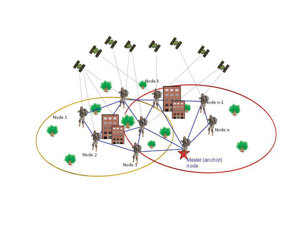
In a larger network, the selection of a sub-network of nodes is an important issue, as in case of a large number of users in the entire network, computational and communication loads may not allow for the entire network to be treated as one entity. Still, information exchange among the sub-networks must be assured.

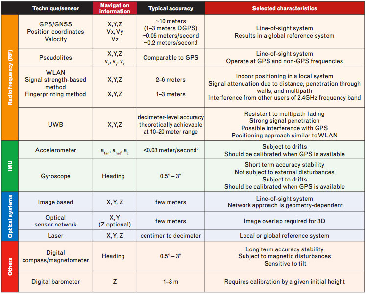
Conceptually, the sub-networks can consist of nodes of equal hierarchy or may contain master (anchor) nodes that normally have a better set of sensors and collect measurements from all client nodes to perform a collaborative navigation solution. Table 1 lists example sensors and techniques that can be used in collaborative navigation.

TABLE 1. Typical sensors for multi-sensor integration: observables and their characteristics, where X,Y,Z are the 3D coordinates, vx, vy, vz are the 3D velocities,

The concept of a master node is also crucial from the stand point of distributed GPS aperture, where it is mandatory to have master nodes responsible for combining the available GPS signals.

Master nodes or some selected nodes will need anti-jamming protection to be effective in challenged electromagnetic (EM) environments. These nodes may have stand-alone anti-jamming protection systems, or can use the signals received by antennas at various nodes for nulling the interfering signals.

Research Challenges

Finding a solution that renders navigation for every GPS user within the network is challenging. For example, within the network, some GPS nodes may have no access to any of the satellite signals, and others may have access to one or more satellite signals. Also, the satellite signals received collectively within the network of users may or may not have enough information to determine uniquely the configuration of the network.

A methodology to integrate sensory data for various nodes to find a joint navigation solution should take into account:
- acquisition of reliable range measurements between nodes (including longer inter-nodal distances);
- limitation of inter-nodal communication (RF signal strength);
- assuring time synchronization between sensors and nodes; and
- limiting computational burden for real time applications.
Distributed GPS Apertures

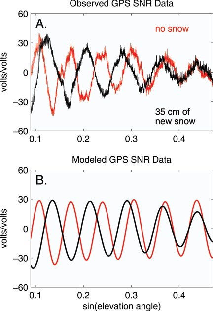
In the case of GPS signal degradation due to increased path loss and radio frequency interference (RFI), one can use an antenna array at the receiver site to increase the gain in the satellite signal direction as well as steer spatial nulls in the interfering signal directions. For a network of GPS users, one may be able to combine the signals received at various receivers (nodes) to achieve these goals (beam pointing and null steering); see Figure 2.

Figure 2. Distributed antenna array.

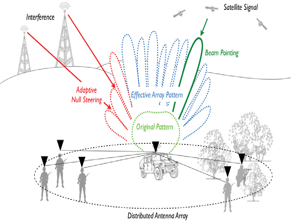
However, a network of GPS users represents a distributed antenna aperture with large (hundreds of wavelengths) inter-element spacing. This large thinned antenna aperture has some advantage and many drawbacks. The main advantage is increased spatial resolution which allows one to discriminate between signals sources with small angular separations. The main drawback is very high sidelobes (in fact, grating lobes) which manifest as grating nulls (sympathetic nulls) in null steering. The increased inter-element spacing will also lead to the loss of correlation between the signals received at various nodes. Thus, space-only processing will not be sufficient to increase SNR by combining the satellite signals received at various nodes. One has to account for the large delay between the signals received at various nodes.

Similarly, for adaptive null steering, one has to use space-time adaptive processing (STAP) for proper operation. These research challenges must be solved for distributed GPS aperture to become a reality:
- Investigate the increase in SNR that can be obtained by employing distributed GPS apertures (accounting for inaccuracies in the inter-nodal ranging measurements).
- Investigate the improvement in the signal-to-interference-plus-noise ratio (SINR) that can be obtained over the upper hemisphere when a distributed GPS aperture is used for adaptive null steering to suppress RFI in GPS receivers. Obtain an upper bound for inter-node distances.
- Based on the results of the above two investigations, develop approaches for combined beam pointing and null steering using distributed GPS apertures.
Inter-Nodal Ranging Techniques

In a wireless sensor network, an RF signal can be used to measure ranges between the nodes in various modes. For example, WLAN observes the RF signal strength, and UWB measures the time of arrival, time difference of arrival, or the angle of arrival. There are known challenges, for example, signal fading, interference or multipath, to address for a RF-based technique to reliably serve as internodal ranging method.

Ranging Based on Optical Sensing. Inter-nodal range measurements can be also acquired by active and passive imaging sensors, such as laser and optical imaging sensors. Laser range finders that operate in the eye-safe spectrum range can provide direct range measurements, but the identification of the object is difficult. Thus, laser scanners are preferred, delivering 3D data at the sensor level. Using passive imagery, such as digital cameras, provides a 2D observation of the object space; more information is needed to recover 3D information; the most typical techniques is the use of stereo pairs or, more generally, multiple-image coverage. The laser has advantages over optical imagery as it preserves the 3D object shapes, though laser data is more subject to artifacts due to non-instantaneous image formation.

In general, regardless whether 2D or 3D imagery is used, the challenge is to recognize the landmark under various conditions, such as occlusions and rotation of the objects, when the appearance of the landmark alternates and the reference point on the landmark needs to be accurately identified, to compute the range to the reference point with sufficient accuracy.

Network Configuration

Nodes in the ad hoc network must be localized and ordered considering conditions, such as type of sensors on the node (grade of the IMU), anti-jamming capability, positional accuracy, accuracy of inter-nodal ranging technique, geometric configuration, computational cost requirements, and so on. There are two primary types of network configurations used in collaborative navigation: centralized and distributed.
- Centralized configuration is based on the concept of server/master and client nodes.
- Distributed configuration refers to the case where nodes in the network can be configured without a master node, that is, each node can be considered equal with respect to other nodes.
Sensor Integration

The selection of data integration method is an important task; it should focus on arriving at an optimal solution not only in terms of the accuracy but also taking the computational burden into account. The two primary options are centralized and decentralized extended Kalman filter (EKF).
- Centralized filter (CF) represents globally optimal estimation accuracy for the implemented system models.
- Decentralized filter (DF) is based on a collection of local filters whose solutions can be combined by a single master filter. DFs can be further categorized based on information-sharing principles and implementation modes.
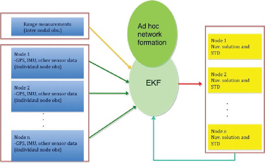
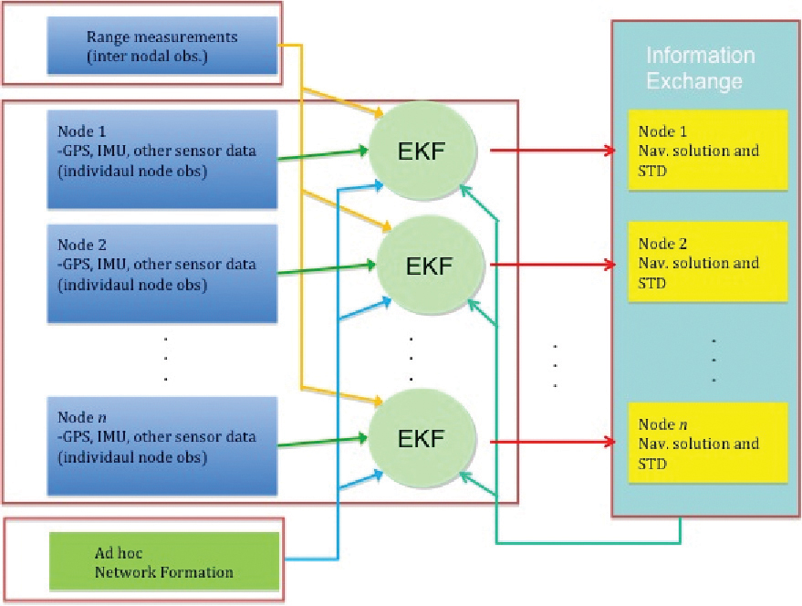
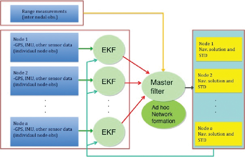
Centralized, Decentralized EKF. These two methods can provide comparable results, with similar computational costs for networks up to 30 nodes. Figures 3–5 describe example architectures of centralized/decentralized EKF algorithms.

In Figure 3, all measurements collected at the nodes and the inter-nodal range measurements are processed by a single centralized EKF. Figures 4 and 5 illustrate the decentralized EKF with the primary difference between them being in the methods of applying the inter-nodal range measurements. The range measurements are integrated with the observations of each node by separate EKF per node in Figure 4, while Figure 5 applies the master filter to integrate the range measurements with the EKF results of all participating nodes.

FIGURE 3. Centralized extended Kalman filter.

FIGURE 4. Decentralized EKF, option 1.

FIGURE 5. Decentralized EKF, option 2.

Performance Evaluation

To provide a preliminary performance evaluation of an example network operating in collaborative mode, simulated data sets and actual field data were used. Figure 6 illustrates the field test configuration, showing three types of nodes, whose trajectories were generated and analyzed.

FIGURE 6. Collaborative navigation field test configuration.

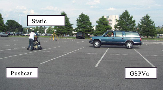
Nodes A1, A2, and A3 were equipped with GPS and tactical grade IMU, node B1 was equipped with GPS and a consumer grade IMU, and node C1 was equipped with a consumer grade IMU only. The following assumptions were used: all nodes were able to communicate; all sensor nodes were time-synchronized; nodal range measurements were simulated from GPS coordinates of all nodes; and the accuracy of GPS position solution was 1–2 meters/coordinate (1s); the accuracy of inter-nodal range measurements was 0.1meters (1s); all measurements were available at 1 Hz rate; the distances between nodes varied from 7 to 70 meters.

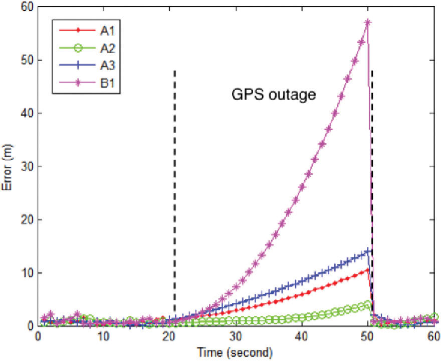
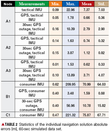
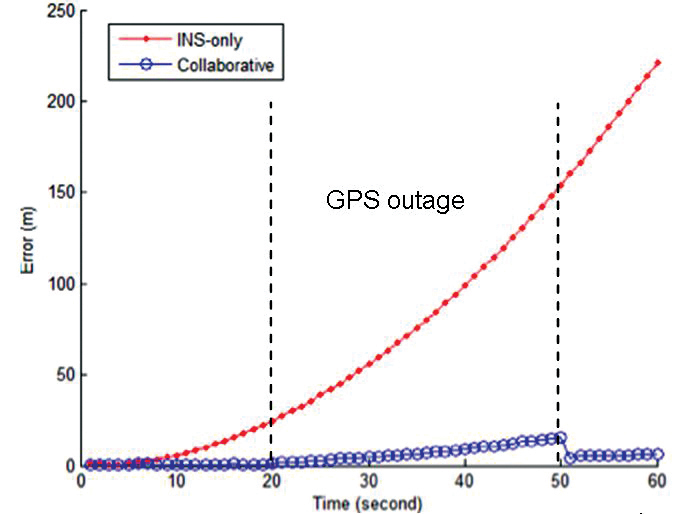
Individual Navigation Solution. To generate the navigation solution for specific nodes, either IMU or GPS measurements or both were used. Since the reference trajectory was known, the absolute value of the differences between the navigation solution (trajectory) and the reference trajectory (ground truth) were considered as the navigation solution error. Figure 7 illustrates the absolute position error for the sample of 60 seconds of simulated data, with a 30-second GPS outage for nodes A1, A2, A3 and B1 (node C1 is not shown, as its error in the end of the test period was substantially bigger than that of the remaining nodes. Table 2 shows the statistics of the errors of each individual node’s trajectory for different sensor configurations.

FIGURE 7. GPS/IMU positioning error for A1, A2, A3, B1 (includes a 30-second GPS outage.)

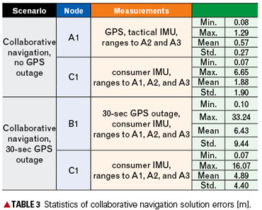
Collaborative Solution. In this example, collaborative navigation is implemented after acquiring the individual navigation solution of each node, which was estimated with the local sensor measurements. The collaborative navigation solution is formed by integrating the inter-nodal range measurements to other nodes in a decentralized Kalman filter, which is referred to as “loose coupling of inter-nodal range measurements.” The test results of different scenarios are listed in Table 3. For cases labeled “30-sec GPS outage,” the GPS outage is assumed at all nodes that are equipped with GPS. The results listed in Table 3 indicate a clear advantage of collaborative navigation for nodes with tactical and consumer grade IMUs, particularly during GPS outages. When GPS is available (see, for example, node A1) the individual and collaborative solutions are of comparable accuracy.

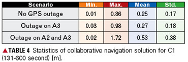
The next experiment used tight coupling of inter-nodal range measurements at each node’s EKF in order to calibrate observable IMU errors even during GPS outages. In addition, varying numbers of master nodes are considered in this example. The tested data set was 600 seconds long, with repeated simulated 60-second GPS gaps, separated by 10-second periods of signal availability. The inter-nodal ranges were ~20 meters.

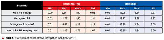
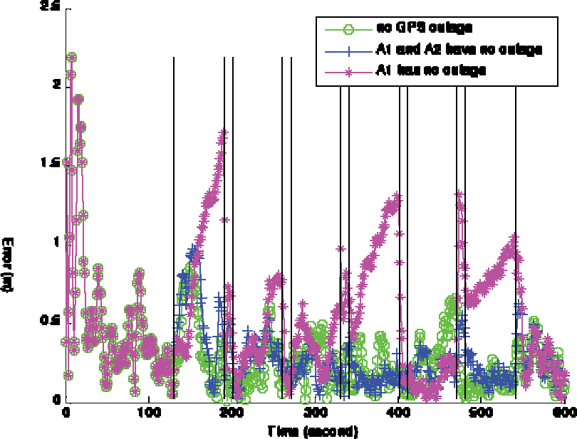
Table 4 and Figure 8 summarize the navigation solution errors for collaborative solution of node C1 equipped with consumer grade IMU only, supported by varying quality other nodes. The error of the individual solution for this node in the end of the 600-second period reach nearly 250 kilometers (2D). Even for the case with a single anchor node (A1), the accuracy of the 2D solution is always better than 2 meters. Another 900-second experimental data with repeated GPS 60-second gaps on B1 node was analyzed with inter-nodal ranging up to 150 meters. Table 5 summarizes the results for C1 node.

FIGURE 8. Absolute error for IMU-only and collaborative navigation solutions of C1 (GPS outage.)

Future Work

Collaborative navigation in decentralized loose integration mode improves the accuracy of a user with consumer grade IMU from several hundreds of meters (2D) to ~16 m (max) for a 30-s GPS gap, depending on the number of inter-nodal ranges and availability of GPS on other nodes. For a platform with GPS and consumer grade IMU (node B1) the improvement is from a few tens of meters to below 10 m.

Better results were obtained when tight integration mode was applied, that is, inter-nodal range measurements were included directly in each EKF that handles measurement data collected by each individual node (architecture shown in Figure 4). For repeated 60-second GPS gaps, separated by 10-second signal availability, collaborative navigation maintains the accuracy at ~1–2 meter level for entire 600 s tested for nodes C1 and B1.

Even though the preliminary simulation results are promising, more extended dynamic models and operational scenarios should be tested. Moreover, it is necessary to test the decentralized scenarios 1 and 2 (Figures 4–5) and then compare them with the centralized integration model shown in Figure 3. Ad hoc network formation algorithm should be further investigated.

FIGURE 9. Absolute errors in collaborative navigation solutions of C1.

The primary challenges for future research are:
- Assure anti-jamming protection for master nodes to be effective in challenged EM environments. These nodes can have stand alone anti-jamming protection system, or can use the signals received by antennas at various nodes for nulling the interfering signals.
- Since network of GPS users, represents a distributed antenna aperture with large inter-element spacing, it can be used for nulling the interfering signals. However, the main challenge is to develop approaches for combined beam pointing and null steering using distributed GPS apertures.
- Formulate a methodology to integrate sensory data for various nodes to obtain a joint navigation solution.
- Obtain reliable range measurements between nodes (including longer inter-nodal distances).
- Assess limitations of inter-nodal communication (RF signal strength).
- Assure time synchronization between sensors and nodes.
- Assess computational burden for the real time application.
Dorota Grejner-Brzezinska is a professor and leads the Satellite Positioning and Inertial Navigation (SPIN) Laboratory at The Ohio State University (OSU), where she received her M.S. and Ph.D. in geodetic science.  Charles Toth is a senior research scientist at OSU’s Center for Mapping. He received a Ph.D. in electrical engineering and geoinformation sciences from the Technical University of Budapest, Hungary. Inder Jeet Gupta is a research professor in the Electrical and Computer Engineering Department of OSU. He received a Ph.D. in electrical engineering from OSU. Leilei Li is a visiting graduate student at SPIN Lab at OSU. Xiankun Wang is a Ph.D. candidate in geodetic science at OSU
September 1, 2010
Innovation: Mobile-phone GPS antennas
Can They Be Better?

By Tony Haddrell, Marino Phocas, and Nico Ricquier

We examine the antenna designs that provide GPS functionality to mobile phones and why most phones still do not provide GPS operation indoors. We also see what it will take to make them better.

INNOVATION INSIGHTS by Richard Langley

WHAT ARE THREE THINGS THAT MATTER MOST for a good GPS signal? Antenna, antenna, antenna. The familiar real-estate adage can be rephrased for this purpose, although the original — location, location, location — is valid here, too.

GPS satellite signals are notoriously weak compared to familiar terrestrial signals such as those of broadcast stations or mobile-phone towers. However, if an appropriate antenna has a clear line-of-sight to the satellite, excellent receiver performance is the norm. But what constitutes an appropriate antenna? The GPS signals are right-hand circularly polarized (RHCP) to provide fade-free reception as the satellite’s orientation changes during a pass. A receiving antenna with matching polarization will transfer the most signal power to the receiver. Microstrip patch antennas and quadrifilar helices, two RHCP antennas commonly used for GPS reception, have omnidirectional (in azimuth) gain patterns with typical unamplified boresight gains of a few dB greater than that of an ideal isotropic RHCP antenna.

But what happens when signals are obstructed by trees or buildings or, worse yet, when we move indoors? Received signal strength plummets. A conventional receiver, even with a good antenna, will then have difficulty acquiring and tracking the signals, resulting in missed or even no position fixes. However, thanks in large part to massive parallel correlation, receivers have been developed with 1,000 times more sensitivity than conventional receivers, permitting operation in restricted environments, albeit usually with reduced positioning accuracy. But such operation requires a standard antenna.

So, do the GPS receivers in our mobile phones now work everywhere? Sadly, no. Consumers demand that their phones not only provide voice communications and GPS but also Bluetooth connectivity to headsets, Wi-Fi, and even an FM transmitter, all in a small form factor at reasonable cost. This requires miniaturizing the GPS antenna and possibly integrating it with the other radio services on the platform. Such compromises can, if the designer is not careful, significantly reduce receiver effectiveness with dramatically reduced antenna gain and distorted antenna patterns. This month we look at some antenna designs providing GPS functionality to mobile phones and examine why most phones still do not provide GPS operation indoors or in other challenging environments. We also find out what it will take to make them better.

“Innovation” is a regular column that features discussions about recent advances in GPS technology and its applications as well as the fundamentals of GPS positioning. The column is coordinated by Richard Langley of the Department of Geodesy and Geomatics Engineering at the University of New Brunswick, who welcomes your comments and topic ideas.

GPS is becoming a must-have feature in mobile phones, with major manufacturers launching new designs regularly, and second-tier manufacturers rapidly catching up. A quick test of any early GPS-equipped phone shows that although the incumbent GPS chip (or chipset) has high sensitivity, the integrated end result cannot perform in low signal conditions. Several challenges facing the phone designer are responsible for this, with the main two being the antenna performance and interference in the GPS band generated within the phone platform itself.

Here we explore the antenna’s role in determining overall performance of the GPS function in a mobile phone, and the potential for avoiding some platform jamming signals by choice of antenna technology.We present some results from an ongoing company study, as part of our remit to assist customers at the system integration level in support of GPS chip sales.

Many handset makers are not GPS or even RF experts, and rely on catalog components to provide their GPS and antenna hardware. Often unsuitable antennas are chosen, or the antennas are integrated in such a way that the original operation mode does not work. Study of a number of candidate phones has shown that, due to the small ground plane available, the antenna component may be merely a band-tuning device, with the ground plane contributing the signal collection function.

At the beginning of 2008, our team launched a project to understand and prioritize the problems for handset makers in the antenna area, and to provide better solutions than those currently in use.

The handset designer faces several problems when incorporating a GPS antenna. First, it has to be very low cost (a few cents, probably). Secondly, it has to be broadly omnidirectional, since there is no knowledge of “up” on a mobile phone, although some manufacturers rely on the fact that location will only be needed when the phone is in the user’s hand or an in-car holder. From the GPS receiver point of view, we would like the antenna to be as far from the communications (transmitting) antenna as possible, and also removed from other transmitting services such as Bluetooth, Wi-Fi, and FM. Users must not be able to detune the antenna out of band by placing their hands on the phone, or by raising the phone to their ears. In a perfect world, they would not obscure an antenna either.

Of course, we would also like to remove some of that platform interference at the antenna stage, and techniques such as differential RF inputs (with a differential antenna) have been proposed in the search for better noise-cancellation performance.

All of this leaves the handset designer with an impossible task, since he has run out of space to fit a decent GPS antenna with all the isolation requirements, and we typically measure GPS antennas that average 26 to 215 dB of gain with respect to a reference dipole, which measures around 21 dB compared to an isotropic antenna when integrated in the handset. Given that a 2 dB loss equates to double the time to fix (in low signal environments) or, alternately, double the amount of baseband signal-search hardware in the GPS chip, it follows that we must exert some effort to help handset integrators implement better antennas. In this respect, some larger manufacturers have in-house projects running, but smaller ones do not have antenna design teams and rely on their suppliers to provide solutions.

So, we start with cataloging the requirements, and given that most current implementations are only in the “mediocre to terrible” class, we look at ways of improving things accordingly. Of course, there are good GPS antenna solutions out there, but handset designers have mostly shunned them on the grounds of cost or even size. Restrictions on these parameters severely hamper the antenna designer, as reducing a GPS L1 antenna below its “natural” size  — about 4 centimeters for a monopole on commonly used FR4-type printed circuit board (PCB) material — inevitably means either using some higher dielectric material, which adds cost, or folding the structure up, which decreases performance.

Single-ended antennas, such as monopoles and microstrip patches, rely on a ground plane, which in a handset is undersized anyway, and is usually difficult to identify and model. True differential designs (such as a dipole) overcome this problem, but are automatically larger. As handsets get smaller and encompass more “connectivity”
(that is, more radio links, including GPS) and competition for antenna space increases, combined antennas become attractive, as they would at least help with the size issue. However, the isolation problems are increased, and since our various radios all (currently) need individual RF inputs, some new layer of complexity and filtering is needed between antenna and chip.

Theory, Performance. We undertook some practical experiments to get a feel for the gap between an antenna’s theoretical performance and its installed performance when integrated with the other phone functions. At present, the idea of modeling all the radiation interactions and mechanical arrangements within such a platform is beyond the scope of the available tools, and so practical measurements are really our only choice in the quest for better antennas.

Finally, we provide some insight into the future, given the rapid advancements driven by mobile-phone technology and the advent of the low-cost handset for new emerging markets. New challenges loom ahead for GNSS antennas, not the least being more bandwidth and multiple frequencies, and we look briefly at what must be done to keep up with handset manufacturers’ requirements in this regard.

Size of the Problem

Location-based services in mobile phones is now an expected function by the more discerning user. With more than 500 million users of such services expected by 2011, pressure on manufacturers to provide ever better user experiences and competition between phone manufacturers will bring pressure on the GPS industry for improved performance. GNSS is now the location technology of choice for mobile phones and will remain so provided that the industry can maintain leadership in cost, size, and performance. FIGURE 1 shows the expected penetration of GNSS (mostly just GPS) in the next few years.

Figure 1. GNSS penetration, mobile phones (Image: Tony Haddrell, Marino Phocas, and Nico Ricquier)

With this many users, the market will soon decide whether the performance is up to expectation or not; this in itself will determine GPS penetration going forward.

Vanishing Space. The first challenge facing the RF antenna designer working on a mobile phone is the size of the whole platform. As the size of the average phone continues to fall, manufacturers are understandably reluctant to increase size again to add new features, such as GPS. Consider the wavelengths of a phone’s various RF services. If the corresponding antennas were implemented as dipoles, the antennas would be bigger than the phone. Clearly the competition for antenna space is high. The designer will want to separate the antennas as much as possible to reduce coupling between them, both in the sense of coupling interference from one service to another (known as isolation) and in the sense of spoiling the pattern (or field) of one antenna with another (interaction).

The chip business addresses the space issue through the advent of combination or combo chips, containing such peripheral services as FM (both receive and transmit), Bluetooth, GPS, and Wi-Fi. While helping with space constraints, this development brings new challenges as these radios have to cohabit the same silicon and still perform individually, whatever the other radios are doing (transmitting music to the car radio using FM while navigating with GPS, for example). It follows that combo antennas similarly save space, but since this might involve simultaneous transmit and GPS receive functions, it is very difficult to achieve the necessary isolation, especially if the user’s body can change the coupling between functions.

FIGURE 2 shows a modern phone with some antennas identified. Not shown is the FM transmit antenna on the rear (the receive function uses the headset cable). One commercially available combo antenna and two custom-made antennas are designed to fit the mechanical layout of the phone. The GPS antenna has been placed at the top of the phone, relegating the communications antenna (really another combo since it handles four frequency bands) to the bottom of the phone, where it is subject to detuning by the user’s hand. The GPS antenna is of the PIFA (planar inverted F antenna) type, working against the ground plane of the main PCB, and is printed on a plastic molding that also implements a loudspeaker and its electrical connections.

Figure 2. Antennas in a mobile phone: 1. GSM/WCDMA antenna, 2.Wi-Fi/Bluetooth combined ceramic chip antenna, 3. GPS antenna (Image: Tony Haddrell, Marino Phocas, and Nico Ricquier)

Size. Until now, we have not looked at the size of GPS antennas. We know that a dipole (on FR4 PCB material) is about 8 centimeters in length, just a little shorter than the average phone platform. Changing to a monopole halves the natural length, but requires an “infinite” ground plane to work against. Ignoring this requirement, some manufacturers simply print a monopole on the main PCB, and put up with the coupling, losses, and pattern deficiencies that arise. Some while ago, we measured the gain of such an arrangement at about 212 dB relative to the reference dipole. So designers have turned to size-reduced antennas, either by using higher dielectric materials to form them, or by using complex shape and feed derivatives (such as the PIFA in Figure 2.)

Another combo idea is to use the communications antenna. In the case shown in FIGURE 3, this is a whip-type antenna on a clamshell-type phone. Although the antenna is free for GPS and uses no additional space, the components to tune the whip for GPS and prevent the transmit bands reaching the GPS low noise amplifier (LNA) add both cost and size. So this is not really too attractive, especially when measurements show a 216 dB performance relative to our dipole, along with a poor coverage pattern. In this model, removing the whip and leaving the ferrule to which it connects provided a 6 dB improvement in performance (for GPS only; obviously it spoils the communications function).

Figure 3. Whip antenna combination (Image: Tony Haddrell, Marino Phocas, and Nico Ricquier)

A more conventional approach is to fit an off-the-shelf GPS antenna. The problem here is that any component-type antenna will have been tested with some standardized ground plane, and most are reliant on the ground plane for both tuning, and pattern and gain. A truly balanced design avoids this problem; FIGURE 4 shows an example. Although these antennas have found favor in personal navigation devices for their superior performance, they are not usually considered for mobile phones because of cost and size considerations. This antenna did, however, give us a reference device against which we could make comparative measurements when undertaking the practical test campaign.

Figure 4. Sarantel miniature volute antenna (Image: Tony Haddrell, Marino Phocas, and Nico Ricquier)

A more usual selection is the patch type, long standard in the GPS industry. One such installation is shown in FIGURES 5 and 6, which offer two views of the same stripped-down phone. The main drawback of this arrangement is the lack of a ground plane visible to the patch antenna, giving both tuning and gain/pattern problems. We measured the gain of this antenna at about 28 dB compared to a dipole antenna connected to the same point in the circuit, which is actually at the better end of the performance range that we see. The designers gave the antenna a position at the top of the phone, as in the Figure 2 phone, but it is still squeezed for space onto the edge of the PCB in favor of the phone’s speakers and the camera components. In this phone, the communications antenna is again at the bottom of the PCB.

Figure 5. Phone with GPS patch antenna at edge of PCB (Image: Tony Haddrell, Marino Phocas, and Nico Ricquier)

Figure 6. Edge view of GPS antenna, top of phone removed. This phone includes an external GPS antenna input connector seen here mounted below the patch antenna. (Image: Tony Haddrell, Marino Phocas, and Nico Ricquier)

Interference and Isolation. The related characteristics of interference and isolation are difficult to specify and model, leading to practical measurements as the only way of accurately characterizing them. Of course, since the mechanical arrangement (including plastics, screen, battery, and PCB components) plays such a large part in determining the levels of interference and isolation, these tests can only be carried out once the phone is at the prototype stage, when major surgery to improve any particular aspect is not really an option. This also creates a problem when considering new approaches, as the result may not resemble the stand-alone tests, unless the antenna element chosen really has no significant interaction with the rest of the phone.

Most interference we see in mobile phones gets into the GPS receiver at the antenna. Typically this is followed by an RF filter of some sort, which although it spoils the noise figure, does eliminate the out-of-band transmissions from the other radios on the platform. Usually we see a plethora of self-generated in-band signals that have entered the GPS receiver via the antenna. Although we can’t filter them out, we can reduce the coupling between antenna and source as much as possible. One effect seen in current offerings is that the GPS antenna may actually be much better at coupling to interferers than it is at extracting GPS signals from free space, thus making the problem worse.

To get a view of the coupling between antennas, we tested a few available phone types to see what was the actual coupling in the antenna band of interest (see TABLE 1). Of course, one advantage of a poor antenna is that its coupling is likely to be less to adjacent antennas. Coupling is also seriously affected by the user holding the phone or the surface on which it is placed. Phones in a pocket seem to be more affected in this way. The table shows measurements with the phone assembled as completely as possible (we have to get connectivity at the antennas) but not being affected by a user or the phone’s environment.

Table: Tony Haddrell, Marino Phocas, and Nico Ricquier

Requirements

To develop requirements for a better antenna implementation, we need to consider the factors discussed above, and to develop numerical specifications against each. Given the variables involving user interaction, mechanical changes from model to model, use cases and the ever-increasing pressure on cost and size, this is far from straightforward. Our team has spent considerable time defining requirements, and a short synopsis is reported here.

In addition to the coexistence requirements (see the next section), the antenna should fulfill the following criteria:
- Minimum cost. The antenna should be of low implementation cost, preferably printed and not requiring complex connectivity to the main PCB, or to require any setup and/or tuning in production;
- Low loss. The GPS industry is used to antennas delivering around 0–3 dB (isotropic) in an upper hemispheric direction. We believe this will not be attainable in a mobile phone, but we set the gain target at an aggressive -4 dB (isotropic);
- Detuning. The antenna must continue to perform to specification with any reasonable detuning environment (such as user handling, pocket, and metal surfaces);
- Mechanical arrangement. The antenna should be of minimum dimensions that can fit the phone mechanics. For example, long and thin may be acceptable along one side of the phone. Also placement near the GPS chip avoids lossy RF tracking;
- Gain pattern. Essentially omnidirectional, accepting that other parts of the phone may cause localized dips in the pattern.
Coexistence and Cohabitation. Initially we aim to define the parameters affecting interaction with other services on the phone platform. By coexistence, we mean the ability to share a platform with the other radios and antennas and only be marginally affected by them, whatever they are doing (such as transmitting full power, low power, or idling, and with any frequency choice). This produces a straightforward immunity table (see TABLE 2) once we have determined the basic isolation between all of the elements. For the purposes of Table 2, we have chosen 15 dB as the minimum isolation value between any two antennas. Obviously there are similar tables for the other functions (GSM, 3G, Wi-Fi, Bluetooth, FM) as well.

Table: Tony Haddrell, Marino Phocas, and Nico Ricquier

A glance at Table 2 will tell the reader that the modern mobile phone implements a vast number of transmit and receive frequencies, modulation types, and standards. Of particular concern to the GPS designer is the advent of wideband CDMA signals, which can cause intermodulation products to appear in band at the intermediate frequency of the GPS receiver. Special receiver techniques are required in this case, but the antenna is unable to help except by being of naturally narrow bandwidth.

Cohabitation is a newer concept that describes the isolation between functions of the same device. In this respect, we are investigating GPS antennas combined with Wi-Fi and Bluetooth services. This is a fairly natural development, since these functions are all add-ons to a conventional phone platform, and there is a space-saving advantage in the combination. Since Wi-Fi and Bluetooth share the same band at 2.4 GHz, they have arrangements internally that allow them to coexist or choose which service is to be used if a clash is inevitable.

As a precursor to forming some specifications, our team measured a commercially available combined antenna, and TABLE 3 shows the isolation results.

Table: Tony Haddrell, Marino Phocas, and Nico Ricquier

The table highlights the need to measure antennas on a representative PCB, since other coupling factors reduce the specified isolation by >6 dB compared to the manufacturer’s reference setup, where the part is the only component on the demonstration board.

Real-Life Testing

A number of tests were carried out on available solutions to gain some information and experience about current offerings and platforms.

At one of our facilities, we have a GTEM (gigahertz transverse electromagnetic) cell, which was constructed in house and has been verified to be working properly (see FIGURE 7). A GTEM cell is an expanded transmission line within which a uniform electromagnetic field can be generated for determining antenna properties such as gain and bandwidth. The internal space at the septum (40 centimeters) is big enough to handle antenna sizes used by GPS. It has a small side door and some feedthroughs (coaxial) to the bottom plate. The RF foam absorbers used inside the GTEM work well at 1.5 GHz (the cell can work from 100 MHz to above 10 GHz).

Figure 7. The GTEM cell and related test equipment (Photo: Tony Haddrell, Marino Phocas, and Nico Ricquier)

Differential vs. Single-Ended Antennas. The first test conducted concerned comparison of balanced and unbalanced antennas, the theory being that a balanced antenna would help with interference because it would be presented to the GPS receiver as a common mode signal (that is, balanced on the positive and negative inputs). The NXP GNS7560 single-chip GPS solution is configurable for single or differential input to the LNA, and was used to conduct the tests.

The trial began with calibration of the test setup using the balanced antenna shown in Figure 4, against which we measured a printed dipole antenna and a monopole equivalent, arranged to incorporate a balun to make it of the same size as the dipole (see FIGURE 8). Once this calibration had been made, we sought to generate an interfering signal on the GPS receiver test board so that comparisons of interference rejection could be made. This was done in two different ways, in case the method of exciting the GPS board was subject to resonances or peculiar standing-wave modes. First, we injected an RF interferer into the power supply via the USB cable that was both powering the GPS board and the communications link to it. The jamming created in this manner was increased until a predetermined drop in GPS sensitivity was reached. A number of frequencies were tried and the results compared. In the second setup, we directly applied an RF signal across the ground plane of the GPS board, using a coaxial feed to excite the ground plane, and repeated the stages described above.

Figure 8. Antennas used in the balanced vs. unbalanced antenna testing (Photo: Tony Haddrell, Marino Phocas, and Nico Ricquier)

Results for both tests were within 2 dB of each other, and showed that the differential approach could reduce local jammer pickup by only 4–6 dB. This is probably due to the differential structure being of similar size to the test platform (chosen to be similar to a phone platform), and therefore not achieving true differential coupling to the on-board radiated jammer. With this marginal advantage, we concluded that the benefit was barely justified by the extra complexity and size involved in differential antennas. Note that this conclusion may be different for smaller (for example, high dielectric) differential antennas, although these are currently not available. We are resolved to revisit this possibility at a later date.

Testing Some Commercial Parts. Having elected to continue in unbalanced-only mode, we tested some commercially available antenna components, which are all aimed at mobile phones and span a range of technologies. Each antenna was tested on its recommended reference design without other mobile phone components or features. However, we did use phone-sized boards, representative plastics, and a real user’s hand in these tests. TABLE 4 shows the comparative results.

Table: Tony Haddrell, Marino Phocas, and Nico Ricquier

For return loss measurements we used a vector network analyzer and a ferrite absorber clamp to suppress cable common-mode effects. For measuring the antenna-received voltage, we used an open-air setup with a horn antenna placed 1 meter away from the DUT (device under test) antenna. The horn is fed with a 100 dBuV 1575 MHz CW signal and the received signal at the DUT is inspected with a spectrum analyzer. The horn is mounted so that we have vertical polarization. Initially, we were only concerned with looking for the maximum attainable voltage and we have positioned the DUT also to vertical polarization. Wooden tables were used to avoid reflections. The last two columns in Table 4 are with plastic in close proximity to the antenna element and the last column is with the plastic grabbed by the hand (as one would grab a phone).

The first thing to note is that of the antennas reported above (which were the best of a bigger number of test pieces) the performance is roughly the same for all of them when configured in their reference mechanical arrangement and not interacting with the phone environment. From the table, we can see that for the particular antenna tested in two positions, its location on the ground plane defines its performance (the ceramic-loaded antenna lost 3 dB in voltage terms when moved to the shorter side of the board). This may be a problem in that the best position performance-wise is not the best for the case where the user interacts with the complete assembly. Also, we see that the user and the plastics have a big effect. In short, the component-type antennas currently available don’t show exciting performance in a real environment, but most are competent GPS antennas when integrated according to their makers’ instructions. However, this is often not possible due to mechanical and other constraints. One drawback of the monopole type of device is its need for a ground-plane-free area underneath the component, and this often conflicts with the requirements of the other antennas, which are looking to maximize the ground plane in the phone.

Novel Approaches, Validation

We started this program to identify the requirements of a good GPS antenna, test some theories and current components, and then develop a new approach. From the foregoing, it is clear that a design that is part of the phone mechanics itself will be better integrated and more predictable in the final implementation. Our design team has begun to model and test some more PCB-centric solutions that attempt to mimic at least the current performance of commercial components, and to minimize the amount of ground-plane loss. We do all our testing on representative (in size and conductivity) phone PCBs. A new approach to thinking about potential arrangements is to use the previously mentioned concept that the whole board is the radiator and the antenna is actually a tuning and feed device. One promising possibility is a slot antenna (or slot feed) formed by removing a small notch of ground plane along the top edge of the phone PCB. Some phones have demonstrated success in forming Bluetooth antennas in this manner, although the lower frequency of GPS does not help.

On a separate path, another idea is to print a PIFA (or similar structure) on the plastics themselves and have it work against the phone ground plane in total. In this case, it is relatively easy to get good performance, but connection of the feed to the main board (where the GPS chipset will be located) is a non-trivial mechanical problem.

Testing of some candidate solutions is under way, and we expect reference designs for customer use to be the deliverable from this work. In addition, it is clear that there is not a one-solution-fits-all conclusion, and that more work will be necessary as phone and GPS designs are further developed.

Acknowledgments

The authors thank the antenna engineering team at NXP’s Mobile and Personal Innovation Center, especially Tony Kerselaers, Felix Elsen, and Norbert Philips who conducted the trials reported here. This article is based on the paper “A New Approach to Cellphone GPS Antennas” presented at ION GNSS 2008.

TONY HADDRELL is a fellow staff architect.

ST-Ericsson in Daventry, England, and a director of iNS Ltd., Weedon, England.

MARINO PHOCAS is an RF systems engineer with ST-Ericsson.

NICO RICQUIER heads the Connectivity Group at NXP Semiconductors in Leuven, Belgium.

Some Mobile Phone Terms

Bluetooth (BT). A communications protocol operating in the 2.4 GHz Industrial, Scientific and Medical (ISM) frequency band, enabling electronic devices to connect and communicate in short-range ad hoc networks.

CDMA. Code division multiple access is a channel access method used by some mobile-phone carriers that allows multiple users to share the same radio frequencies using spread spectrum signals.

DCS1800. Digital Cellular Service version of GSM operating in the 1700 and 1800 MHz bands.

EDGE. Enhanced Data Rates for GSM Evolution, a third-generation (3G) version of GSM.

EGSM900. The Extended GSM 900 MHz band.

FDD. Frequency-division duplexing, a communications protocol that uses different carrier frequencies for transmitt
ing and receiving.

FM. The broadcast frequency modulation band.

GMSK. Gaussian minimum shift keying, a continuous-phase frequency-shift keying modulation scheme used for GSM communications.

GSM. Global System for Mobile communications, the most popular mobile phone standard.

GSM850. A GSM version operating in the 800 MHz band.

PCS1900. Personal Communications Service version of GSM operating in the 1800 and 1900 MHz bands.

QPSK. Quadrature phase-shift keying. A modulation technique used in CDMA systems.

Triplexer. A filtering device to provide isolation between communications and GPS circuits when sharing an antenna.

W-CDMA. Wideband CDMA, an enhanced, 3G version of CDMA.

Wi-Fi 802.11b/g. Wi-Fi describes a standard class of wireless local area network (WLAN) protocols based on the IEEE 802.11 standards operating primarily in the 2.4 GHz band.

FURTHER READING

• Mobile Phone Development

“The Smartphone Revolution” by F. van Diggelen in GPS World, Vol. 20, No. 12, December 2009, pp. 36–40.

• Signal Compatibility Issues

“Jammers – the Enemy Inside!” by M. Phocas, J. Bickerstaff, and T. Haddrell in Proceedings of ION GNSS 2004, the 17th International Technical Meeting of the Satellite Division of The Institute of Navigation, Long Beach, California, September 21–24, 2004, pp. 156–165.

• High Sensitivity GPS Receiver

“A Single Die GPS, with Indoor Sensitivity – the NXP GNS7560” by T. Haddrell, J.P. Bickerstaff, and M. Conta in Proceedings of ION GNSS 2008, the 21st International Technical Meeting of the Satellite Division of The Institute of Navigation, Savannah, Georgia, September 16–19, 2009, pp. 1201–1209.

• Mobile Phone GPS Antennas

“A Compact Broadband Planar Antenna for GPS, DCS-1800, IMT-2000, and WLAN Applications” by R. Li, B. Pan, J. Laskar, M.M. Tentzeris in IEEE Antennas and Wireless Propagation Letters, Vol. 6, 2007, pp. 25–27 (doi:10.1109/LAWP.2006.890754).

“Getting into Pockets and Purses: Antenna Counters Sensitivity Loss in Consumer Devices” by B. Hurte and O. Leisten in GPS World, Vol. 16, No. 11, November 2005, pp. 34–38.

“Miniature Built-in Multiband Antennas for Mobile Handsets” by Y.X. Guo, M.Y.W. Chia, and Z.N. Chen in IEEE Transactions on Antennas and Propagation, Vol. 52, No. 8, August 2004, pp. 1936–1944 (doi: 10.1109/TAP.2004.832375).

“Mobile Handset System Performance Comparison of a Linearly Polarized GPS Internal Antenna with a Circularly Polarized Antenna” by V. Pathak, S. Thornwall, M. Krier, S. Rowson, G. Poilasne, L. Desclos in Proceedings of IEEE Antennas and Propagation Society International Symposium 2003, Columbus, Ohio, June 22-27, 2003, Vol. 3, pp. 666–669 (doi:10.1109/APS.2003.1219935).

Planar Antennas for Wireless Communications by K.L. Wong, published by John Wiley & Sons, New York, 2003.

• Basics of GPS Antennas

“GNSS Antennas: An Introduction to Bandwidth, Gain Pattern, Polarization, and All That” by G.J.K. Moernaut and D. Orban in GPS World, Vol. 20, No. 2, February 2009, pp. 42–48.

“A Primer on GPS Antennas” by R.B. Langley in GPS World, Vol. 9, No. 7, July 1998, pp. 50–54.
February 1, 2010
On the Edge: Multipath Measures Snow Depth

The September “Innovation” column in this magazine,  “It’s Not All Bad: Understanding and Using GNSS  Multipath,” by Andria Bilich and Kristine Larson, mentions the use of multipath in studying soil moisture, ocean altimetry and winds, and snow sensing. An  experiment the authors conducted, designed to study soil moisture, yielded a surprise bonus: a new methodology for measuring snow depth via GPS multipath. It has important implications for weather and flood forecasting, and could also bring new insight to bear on GPS antenna design.

In the “Innovation” column, the authors wrote, “Motivated by our studies showing that multipath effects could clearly be seen in geodetic-quality data collected with multipath-suppressing antennas, we proposed that these same GPS data could be used to extract a multipath parameter that would correlate with changes in the reflectance of the ground surface. . . .

“We carried out an experiment designed to more rigorously demonstrate the link between GPS signal-to-noise ratio (SNR) and soil moisture. Specifically, we were interested in using GPS reflection parameters to determine the soil’s volumetric water content — the fraction of the total volume of soil occupied by water, an important input to climate and meteorological models. Traditional soil moisture sensors (water content reflectometers) were buried in the ground at multiple depths (2.5 and 7.5 centimeters) at a site just south of the University of Colorado.”

Here Comes the Storm. During the experiment, two late-season snowstorms swept over Boulder. Larson and colleagues discovered that changes in multipath clearly correlated with changes in the snow’s depth, as measured by hand and with ultrasonic sensors at the test site. While it has been long recognized that snow can affect a GPS signal, this demonstrates for the first time that a standard GPS receiver, antenna, and installation — deliberately designed to suppress multipath — can be used to measure snow depth.

On September 11, Geophysical Research Letters, published by the American Geophysical Union, featured an article titled “Can We Measure Snow Depth with GPS Receivers?” by Larson and Felipe Nievinski of the Department of Aerospace Engineering Sciences, University of Colorado; Ethan Gutmann and John Brown of the National Center for Atmospheric Research; Valery Zavorotny of the National Oceanic and Atmospheric Administration; and Mark W. Williams, from UC’s Department of Geography, all based in Boulder.

The authors adapted an algorithm used for modeling GPS multipath from bare soil to predict GPS SNR for snow, introducing a uniform planar layer of the snow on the top of soil. The algorithm treats both direct and surface-reflected waves at two opposite circular polarizations as plane waves that sum up coherently at the antenna. They write:

“The amplitude and the phase of the reflected wave is driven by a polarization-dependent, complex-value reflection coefficient at the upper interface of such a combined medium with a known vertical profile of the dielectric permittivity e. The reflection coefficient is calculated numerically using an iterative algorithm in which the medium is split into sub-layers with a constant e. For the soil part, we use a known soil profile model that depends on the soil type and moisture. For frozen soil, soil moisture (liquid water) is low, as for very dry soil. For the snow part, we take a constant profile with e, considering relatively dry and wet snow layer thicknesses.

“After calculating the complex amplitude of the reflected wave at each polarization, we multiply it by a corresponding complex antenna gain. The same procedure is applied to the complex amplitude of the direct wave. After that, the modulation pattern of the received power, or the SNR, as a function of the GPS satellite elevation angle is obtained by summing up coherently all the signals coming from the antenna output and taking the absolute value square of the sum.”

Figure 1(a) shows GPS SNR measurements for one satellite on the day immediately before and the day immediately after an overnight snowfall of 35 centimeters (roughly 10 inches). Figure 1(b) shows the corresponding model predictions for multipath. The two figure  portions amply demonstrate that the multipath has a significantly lower frequency if snow is present as compared with bare soil. The authors further noted that the model amplitudes do not show as pronounced a dependence on satellite elevation angle as the observations, and state the necessity of further work on antenna gains in order to use model amplitude predictions.

Figure 1. (a) GPS SNR measurements for PRN 7 observed at Marshall GPS site on days 107 (red) and 108 (black) after direct signal component has been removed. Approximately 35 centimeters of snow had fallen by day 108. (b) Model predictions for GPS multipath from day 107 with no snow on the ground (red), and day 108 after 35 centimeters of new snow fall had accumulated (black) using an assumed density of 240 kg m-3 (figures reproduced by permission of American Geophysical Union).

How Deep the Snow. The authors propose that the hundreds of geodetic GPS receivers operating in snowy regions of the United States, originally installed for plate deformation studies, surveying, and weather monitoring, could also provide a cost-effective means to estimate snow depth.

Currently, a few conventional monitor points measure snow depth, but only at that point, and the data does not extrapolate well. Snow forms an important component of the climate system and a critical storage component in the hydrologic cycle. Accurate data of the amount of water stored in the snowpack is critical for water supply management and flood control systems. As more snow falls at higher elevations, varying greatly even within one valley or watershed, current remote-sensing snow monitors do not supply adequate data. Further, snow may be redistributed by wind, avalanches, and non-uniform melting, so that continuous data would be very helpful.

Using GPS multipath to map snow depth could improve watershed analyses and flood prediction — and, carried steps further, produce data to help better understand multipath, bringing innovation to future antenna designs.

FIGURE 2. Snow depth derived from GPS (red squares), the three ultrasonic snow depth sensors (blue lines), and field measurements (black diamonds). Bars on field observations are one standard deviation. GPS snow-depth estimates during the first storm (doy 85.5–86.5) are not shown (gray region) because the SNR data indicate that snow was on top of the antenna.

Kristine Larson was featured as one of the “50 GNSS Leaders to Watch” in the May 2009 issue of GPS World.

Manufacturer

For the experiment a Trimble NetRS receiver was used with a TRM29659.00 choke-ring antenna with SCIT radome, pointed at zenith.

November 1, 2009
Antenna-Induced Biases in GNSS Receivers

By Inder Jeet Gupta

It is well known that the phase center of a GNSS antenna can vary with the satellite direction. This phase center movement leads to aspect dependent carrier phase and code phase biases in the satellite signal. For precise geo-location, one needs to characterize the antenna-induced carrier and code phase biases over the upper hemisphere. In the case of fixed pattern antennas (the antenna pattern does not vary with the incident signal environment) one can characterize the antenna induced biases a priori and use the data for corrections in the field. This is a standard practice in the surveying community.

For antennas used with AJ (Anti-Jam) systems, however, a priori characterization of the antenna induced biases may not be of much value. These antennas consist of multiple elements. The signals received by various antenna elements are weighted and then summed together to form the composite output signal. The element weights depend on the incident signal (mainly interfering signal) scenario. As the incident signal scenario changes so do the individual antenna element weights which in turn will lead to different values for antenna induced carrier phase and code phase biases.

As illustration, Figure 1 shows the antenna induced code phase bias of an AJ antenna over the upper hemisphere in the absence of all interfering signals as well as in the presence of two interfering signals.

Figure 1. Antenna induced code phase bias (in meters) over the upper hemisphere. Left: no interfering signal; right: two interfering signals.

In the figure, the center of the circle corresponds to the zenith and the outer ring corresponds to the horizon. The antenna induced code phase bias is plotted using a color scale in meters. Note that even in the absence of interfering signals, the antenna induced bias varies with the aspect angle. The presence of the interfering signals affects the antenna induced biases. This is true in the angular region surrounding the interfering signals as well as in the angular region away from the interfering signals.

One can observe this more clearly in Figure 2 where the difference between the antenna induced code phase biases in the absence of interfering signals and in the presence of interfering signals is plotted using a color scale in centimeters. Note that the difference in the antenna induced code phase bias is quite significant, and one may not be able to obtain precise location without proper corrections.

Figure 2. Difference (in cm) between the antenna-induced code phase bias in the presence of two interfering signals and in the absence of the interfering signals.

The question is what could be done to minimize the effects of adaptive antenna induced biases in GNSS receivers. In my opinion, one can take the following two approaches. In the first approach (see reference), one predicts the antenna-induced biases on the fly. This approach requires knowledge of in situ volumetric patterns of individual elements of an AJ antenna over the bandwidth of GNSS signals as well as access to the antenna element weights. With a perfect knowledge of these quantities, one can come up with a very good prediction and can correct for the antenna induced biases. The sensitivity of the prediction to various parameters, however, needs to be studied.

The second approach would be to develop novel weighting algorithms for GPS receiver adaptive antennas. Note that the current algorithms are mostly designed to either steer nulls in the interfering signal directions or maximize carrier to noise ratio in some sense. These novel algorithms should not only lead to improved carrier to noise ratio in the presence of interfering signals but should also make sure that the antenna-induced biases do not vary from their values in the absence of all interfering signals.

Further, these algorithms should not use many degrees of freedom to meet the various constraints in that GNSS AJ antennas do not have many degrees of freedom. If most of the degrees of freedom are consumed to meet the above constraints then one will not have enough degrees of freedom left to null the interfering signals. This is a very challenging task, but leads to a good research problem!

Inder J. Gupta

Ohio State University

References

I.J. Gupta, et. al., Prediction of antenna and antenna electronics induced biases in GNSS receivers, Proceedings of ION 2007 National Technical Meeting, San Diego, CA, January 2007.

May 17, 2007