Tag: David B. Zilkoski

Discussing the new North American-Pacific Geopotential Datum of 2022 — Part 1

On April 24-25, 2017, the National Geodetic Survey (NGS) hosted the 2017 Geospatial Summit in Silver Spring, Maryland, to discuss its plans for replacing the North American Datum of 1983 (NAD 83) and the North American Vertical Datum of 1988 (NAVD 88) in 2022.

The summit was a day and a half long and provided an opportunity for NGS to share updates and discuss the progress of projects related to National Spatial Reference System (NSRS) Modernization. Stakeholders across the federal, public and private sectors also provided feedback and impacts of New Datums on their products and services.

The absolute differences between the new vertical reference frame, North American-Pacific Geopotential Datum of 2022 (NAPGD2022), and NAVD 88 are going to be large but, in most regions of the country, the relative differences over small areal extents will be small.

NGS is developing geodetic routines and tools to transform heights from NAVD 88 to NAPGD2022, and to facilitate the incorporation of geodetic leveling data into NAPGD2022 to establish NAPGD2022 heights. To prepare for the new datums and develop implementation plans, stakeholders should obtain an understanding of the differences between NAPGD2022 and NAVD 88.

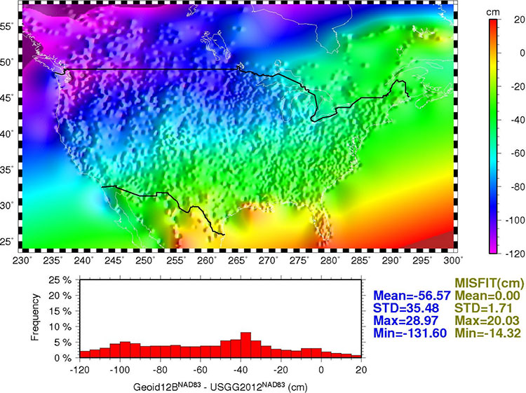
My previous columns provided figures that demonstrated the approximate differences between NAPGD2022 and NAVD 88 heights at a national level. (See figure 1.) This column will provide feedback from stakeholders that participated in the Geospatial Summit and, using NGS’ GPS on BMs dataset, a discussion on the differences between NAPGD2022 and NAVD 88 (and NGVD 29) at a local level.

Figure 1 – Approximate Change Between NAPGD2022 and NAVD 88 Using GPS on BMs Data (units = cm). (Image: National Geodetic Survey)

Information about the summit and Summit Documents can be downloaded here.

Read an excerpt from website here.

If you check on the tab titled “Summit Documents” you can download the agenda and documents provided to participates. Read excerpts from the summit here.

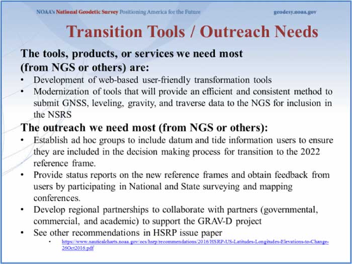
The first day consisted of presentations by NGS leadership and personnel providing updates and discussing the progress of projects related to the NSRS modernization. The presentations by NGS employees can be downloaded from NGS’ presentations library at this web link. View an excerpt from NGS’ presentations library here.

The afternoon of day 2 were presentations by partners and stakeholders. (See box titled “Excerpt from NGS 2017 Geospatial Summit Agenda – Afternoon of Day 2.”)

Excerpt from NGS 2017 Geospatial Summit Agenda – Afternoon of Day 2
Day 2 Afternoon Agenda from NGS’ 2017 Geospatial Summit
Day 2: Tuesday, April 25, 20171:30 – 3:05 Impacts of New Datums on Programs and Partners (Part 1)
Coastal Mapping Program and VDatum: Mike Aslaksen and Stephen White, NOAA/NGS
Federal Emergency Management Agency (FEMA): Kimberly Pettit, FEMA
U.S. Geological Survey (USGS): Kari Craun, USGS
U.S. Army Corps of Engineers (USACE): Jim Garster, USACE
National Geospatial-Intelligence Agency (NGA): Stephen Malys, NGA
3:05 – 3:25 Break
3:25 – 4:55 Impacts of New Datums on Programs and Partners (Part 2)
Geospatial and Remote Sensing Customers: Amar Nayegandhi, Dewberry
Geographic Information System (GIS) Customers: Kevin Kelly, Esri
Global Navigation Satellite System (GNSS) Equipment Customers: Hamid Mahmoudabadi, Trimble Kyle Snow, Topcon
State Government Partners: Gary Thompson, N.C. Department of Public Safety
Local Government Partners: Vickie Anglin, Fairfax County Government, Virginia; Patrick Simon, Baltimore County Land Survey, Maryland
4:55 – 5:00 Wrap-up and closing

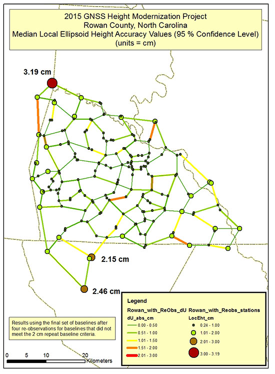
In order for consistency, NGS provided guidance and a set of template slides for guest presenters to use. Guest presenters were allotted 10 minutes to present and limited to four slides. The presentation by the guest presenters are not on NGS’ Presentations Library but I’ve been told that they will be available on the Summit website later this year. Gary Thompson, Chief of the North Carolina Geodetic Survey (NCGS), provided me a copy of his slides and gave me permission to include them in this column. (See box titled “Power point Slides Presented by Gary Thompson, Chief of NCGS, at the NGS 2017 Geospatial Summit.”) North Carolina has been very proactive in addressing the impacts of the new datums on NC products and services. North Carolina Geodetic Survey has established a North Carolina Geodetic Survey Advisory Committee that reviews NCGS products and services, and they have established the North Carolina 2022 Reference Frame Working Group to prepare for the new datums.

Slide: National Geodetic Survey

Powerpoint slides presented by Gary Thompson, chief of NCGS, at the NGS 2017 Geospatial Summit

All of the presentations by the invited guest speakers were interesting, and everyone followed NGS’ guidance which helped to focus the Summit on the main issues associated with a datum change. As expected, each stakeholder had their own set of issues and concerns about transitioning to a datum. The following are some common themes that I heard from the participants:

(1) There are a lot of products and services that will be effected by a datum change,
(2) An official transformation model between the old and new datum(s) published by NGS is critical for a successful transition to a new datum,
(3) Guidance documents that are “easily” understood by “non-geodesists” is required for a smooth implementation of a new datum, and
(4) More frequent geospatial summits and webinars are needed to provide updates on the status of the projects associated with NSRS modernization and to ensure user involvement in the process.

I contacted a couple of the guest presenters to discuss their feedback on the New Datums. As NAVD 88 Program Manager, I collaborated with many of them during the development and implementation of the NAVD 88. As in the transition from NGVD 29 to NAVD 88, it’s not the conversion of coordinates that’s a problem; a good transformation tool should meet that requirement. Saying that, it was stated that many users rely on commercial and open source software to convert their data, so they would like NGS to collaborate with others to ensure that these software suppliers are using the appropriate algorithms/information in their products. The integration with legacy data referenced to older datums may be complicated for some products and services; therefore, the process of transforming each product and service will need to be addressed individually. If all data are in digital form with the appropriate metadata, then the transformation should be relatively easy to accomplish and maps with new contour lines or new base flood elevations referenced to the new datum could be generated. However, how these new maps are integrated with old maps is a different issue. I will address some of these potential issues in future columns.

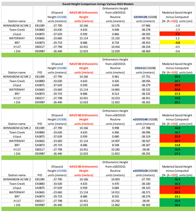
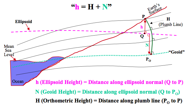
To prepare implementation plans, users must obtain a working knowledge of the differences between the old and new datums. As previous mentioned, the absolute differences between the new vertical reference frame, NAPGD2022, and NAVD 88 are going to be large but, in most regions of the country, the relative differences over small areal extents will be small. To evaluate the relative differences at the local level, the differences between NAPGD2022 and NAVD 88 (and NGVD 29) were computed for bench marks in the NGS’ GPS on BMs dataset. The NAD 83 (2011) latitude, longitude, and ellipsoid height of each station was transformed to the IGS08 reference frame using NGS’ HTDP web tool, and then the GNSS-derived orthometric height was computed using the following formula:

Approximate NAPGD2022 GNSS-Derived Orthometric Height
Equals
IGS08 Ellipsoid Height minus xGeoid16b Geoid Height (referenced to IGS08).

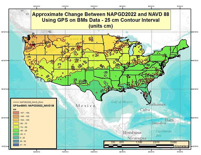
Figure 1 is a plot of the difference between the approximate NAPGD2022 height and the published NAVD 88 height for bench marks that are part of the GPS on BMs dataset and have the published attribute of “Adjusted.” It should be noted that these are only estimated changes because the final NAPGD2022 reference frame will not be exactly the same as the current IGS08 reference frame, but these estimates should serve the purpose of providing approximate changes for users to develop transition plans.

Since some users are still converting NGVD 29 heights to NAVD 88 heights, the approximate change between NAPGD2022 and NGVD 29 is provided in figure 2. VERTCON values were used to convert the NAVD 88 published heights to NGVD 29 heights, and then the difference between the approximate NAPGD2022 orthometric height and the NGVD 29 orthometric height was computed.

Figure 2 – Approximate Change Between NAPGD2022 and NGVD 29 Using GPS on BMs Data (units = cm). (Image: National Geodetic Survey)

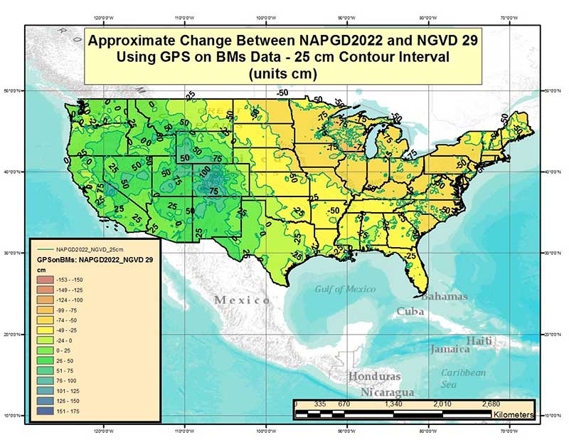
As shown in figure 2, the absolute differences between the new vertical reference frame, NAPGD2022, and NGVD 29 are also going to be large but, once again, in most regions of the country, the relative differences over small areal extents will be small.

What does this look like in a local area? Figure 3 is a plot of the approximate change between NAPGD2022 and NAVD 88 in North Carolina and surrounding states, and figure 4 is plot of the approximate change between NAPGD2022 and NGVD 29 in North Carolina and surrounding states.

Figure 3 – Approximate Change Between NAPGD2022 and NAVD 88 in North Carolina and Surrounding States Using GPS on BMs Data (units = cm). (Image: National Geodetic Survey)

Figure 4 – Approximate Change Between NAPGD2022 and NGVD 29 in North Carolina and Surrounding States Using GPS on BMs Data (units = cm). (Image: National Geodetic Survey)

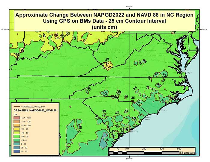
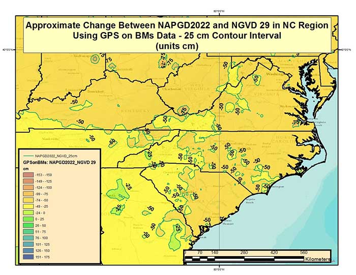
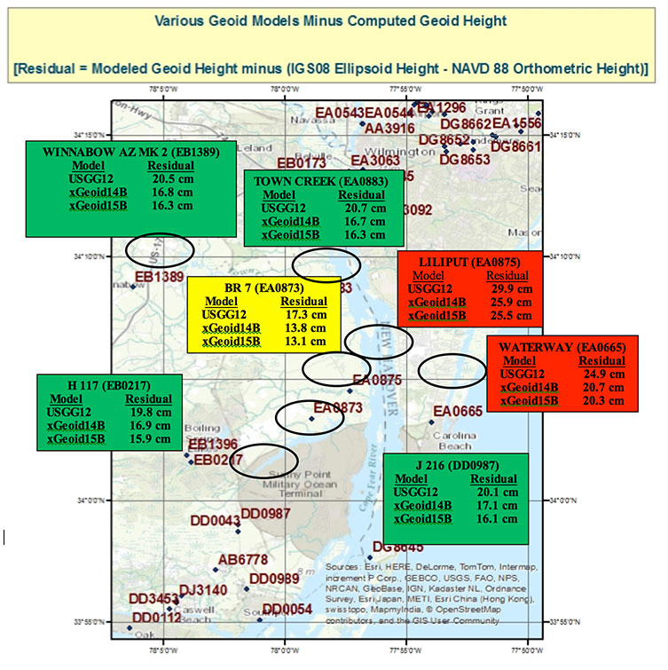
Figure 5 provides a more detailed depiction of the change between NAPGD2022 and NAVD 88 along the North Carolina Atlantic Coast. The differences appear to vary by several centimeters but some of these differences are due to errors in published heights (both ellipsoid and orthometric). These differences can be used to develop a transformation model but the user will need to know the accuracy of the model, globally and locally.

Figure 5 – Approximate Change Between NAPGD2022 and NAVD 88 along North Carolina Atlantic Coast Using GPS on BMs Data (units = cm). (Image: National Geodetic Survey)

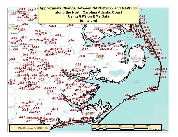
Figure 6 is a detailed depiction of the change between NAPGD2022 and NGVD 29 in the same area as shown in figure 5. Comparing figures 5 and 6, the reader should notice that the differences between NAPGD2022 and NGVD 29 are about 30 cm larger (more negative) than the differences between NAPGD2022 and NAVD 88.

Figure 6 – Approximate Change Between NAPGD2022 and NAVD 29 along North Carolina Atlantic Coast Using GPS on BMs Data (units = cm). (Image: National Geodetic Survey)

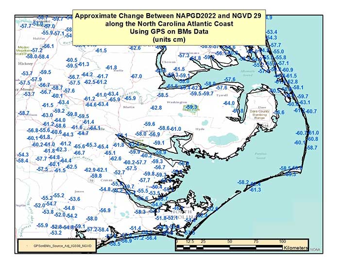
Figure 7 is the difference between NAPGD2022 and NAVD 88 in western North Carolina. The local difference in the NC mountains is around -35 cm which is about 10 cm different from the NC Atlantic Coast. Questions that users need to address include: What is the accuracy of the transformation model? And What is the accuracy of the product or service being transformed? The transformation model will not replace the original survey results but may be useful for transforming some products and services.

Figure 7 – Approximate Change Between NAPGD2022 and NAVD 88 in the Western North Carolina Using GPS on BMs Data (units = cm). (Image: National Geodetic Survey)

Table 1 provides the average difference between NAPGD2022 and NAVD 88 (and NGVD 29) by State using the GPS on BMs dataset. This table shows that there are large differences between NAPGD2022 and both NGVD 29 and NAVD 88. No matter which datum the product or service is referenced to, it will probably need to be transformed to NAPGD2022.

Table 1 – Average Difference Between NAPGD2022 and NAVD 88 (and NGVD 29) by State Using GPS on BMs Dataset (units = cm). Click to enlarge. (Date: National Geodetic Survey)

Average Difference Between NAPGD2022 and NAVD 88 by State Using GPS on BMs Dataset (units = cm). Click to enlarge. (Date: National Geodetic Survey)

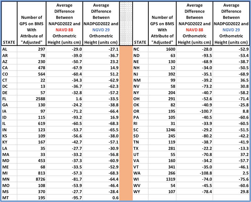
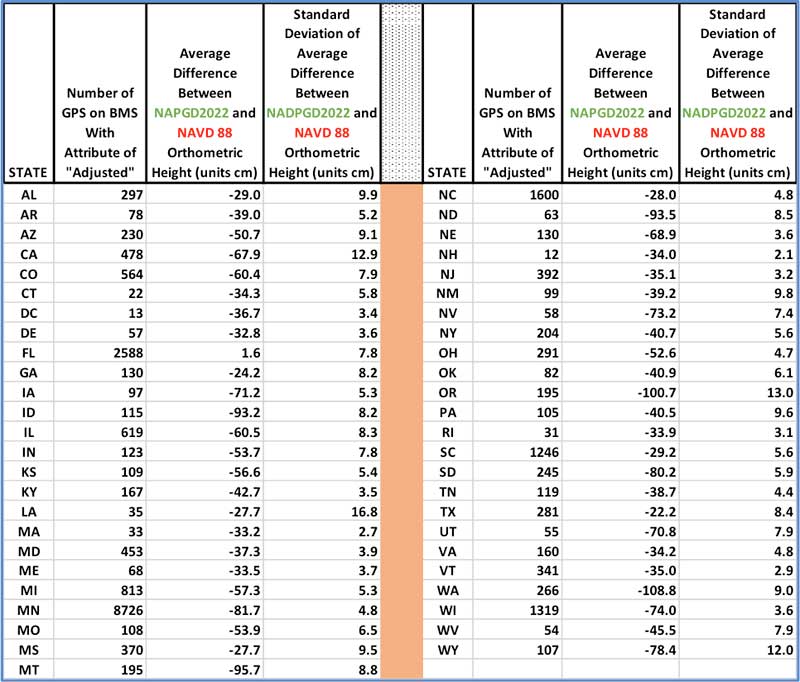
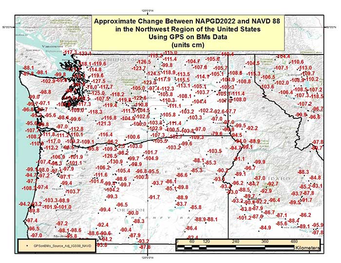
Table 2 provides the standard deviation of the average difference between NAPGD2022 and NAVD 88 by State. For example, North Carolina has a sample size of 1600 stations and its average difference is -28 cm with a standard deviation of 4.8 cm. Looking at figures 5 and 7, there appears to be a difference of 10 cm across the State. The States in the northwestern region of the United States have a larger difference between NAPGD2022 and NAVD 88 as well as a larger standard deviation. Oregon has a sample size of 195 stations and its average difference is -100.7 cm with a standard deviation of 13.0 cm, and Washington has a sample size of 266 stations and its average difference is -108.8 cm with a standard deviation of 9.0 cm. Figure 8 is a plot of the approximate change between NAPGD2022 and NAVD 88 in the northwest region of the United States.

As mentioned previously, these differences will vary from station to station because of a bias and trend between the two datums and due to remaining errors in published heights (both ellipsoid and orthometric). As I have noted in previous columns, many of the large relative differences between stations in a local area could be due to an invalid NAVD 88 published height because the bench mark moved since the last time the height of the bench mark was adjusted and published, and/or an undetected error in an ellipsoid height due to a weak GNSS project design. Either way, in my opinion, most of these stations with large relative differences don’t accurately represent the current NAVD 88. NGS’ modernization of the NSRS will provide a more accurate and consistent reference frame, and improve the user’s ability to obtain a current and accurate orthometric height.

Figure 8 – Approximate Change Between NAPGD2022 and NAVD 88 in the Northwest Region of the United States Using GPS on BMs Data (units = cm). (Image: National Geodetic Survey)

This column highlighted some of the feedback provided by guest presenters at the NGS’ 2017 Geospatial Summit held on April 24-25, 2017, in Silver Spring, Maryland. The column also provided a discussion on the approximate differences between NAPGD2022 and NAVD 88 (and NGVD 29) at a national and local level. To prepare for the new datums and develop implementation plans, users should obtain an understanding of the differences between NAPGD2022 and NAVD 88. This column is the first in a new series of columns addressing topics associated with transitioning to the new North American -Pacific Geopotential Datum of 2022 (NAPGD2022).

June 7, 2017

A look at NGS’ GPS on benchmarks program in Alaska

The last column, February 2017, focused on addressing the following questions: (1) Is the large GPS on benchmarks residual due to an issue with the NAVD 88 orthometric height or the NAD 83 (2011) ellipsoid height? and (2) Should stations with large GPS on benchmarks residuals be included in the development of NGS’ hybrid geoid models? The column provided suggestions on how users can assist NGS in determining the reason for the large difference between the modeled hybrid geoid value and computed GNSS/leveling geoid computed value. It was mentioned that this information will be useful to NGS when developing hybrid geoid models and the 2022 Vertical Transformation model. My previous columns have focused on the conterminous United States. This column is going to discuss the GPS on benchmarks residuals for the state of Alaska.

The February 2017 column noted that many of these large GPS on BM residuals could be due to an invalid NAVD 88 published height because the benchmark moved since the last time the height of the benchmark was adjusted and published, and/or an undetected error in an ellipsoid height due to a weak GNSS project design. The State of Alaska is very large; it has a sparse leveling network, and benchmarks are subject to movement due to ground conditions, isostatic effects, and seismic activity. The Geophysical Institute at the University of Alaska, Fairbank, has a lot of interesting reports on the movement in Alaska. Many of these stations would be identified as benchmarks with invalid heights when users follow Federal geodetic survey guidelines, procedures, and specifications. Benchmarks with invalid heights would not be used in controlling geodetic surveys and, in my opinion, should not be used in the hybrid geoid model. As I mentioned in my previous columns, this is not meant to be a criticism of NGS process for creating their hybrid geoid model. NGS’ goal is to create a hybrid geoid model that is consistent with published NAVD 88 values. I believe NGS is using all the data and information available to them. A goal of my last column was to emphasize to users the importance to strategically occupy stations to help support the GPS on benchmarks program which will result in the creation of a hybrid geoid model that accurately represents the current NAVD 88.

First, let’s look at the leveling network design of Alaska. Figure 1 depicts the leveling network design used to establish heights in the NAVD 88. The figure indicates that most of the leveling data used in NAVD 88 was between 1965 and 1975. It should be noted that a major releveling project was performed in 1965 after the 1964 Good Friday Alaska Earthquake. There were some short leveling lines performed in the late 1980s and early 1991s. These data are now old and the question about whether the NAVD 88 height of the benchmark is still valid must be addressed.

Alaska is prone to both episodic crustal motion (i.e. earthquakes) and the effects of long-term isostatic adjustment, which makes maintaining accurate vertical control difficult at best. (See figure 2 for a plot of earthquakes in Alaska). The 1964 Good Friday Alaska Earthquake, a magnitude of 9.2, changed heights as much as 8 feet. In addition to the initial damage at the time of the earthquake, there’s a post seismic vertical deformation movement that occurred. Suito and Freymueller (2009) provided a postseismic deformation model predictions for the 1964 earthquake [see box titled “Postseismic Velocity Predictions from Suito and Freymueller (2009)]”. An ArcGIS raster layer was developed using the grid values obtained from the website. Figure 3 is a plot of the vertical deformation model using Suito and Freymueller’s gridded dataset.

Postseismic Velocity Predictions from Suito and Freymueller (2009)

This page provides access to postseismic deformation model predictions for the 1964 earthquake. The model includes afterslip and viscoelastic relaxation (including the viscoelastic response to the afterslip), for the best-fit model derived by Suito and Freymueller (2009). That model includes a realistic slab geometry and a uniform asthenospheric relaxation time of 20 years. The full reference for the paper and the model is given below:
Suito, H., and J. T. Freymueller, A viscoelastic and afterslip postseismic deformation model for the 1964 Alaska earthquake, J. Geophys. Res., doi:10.1029/ 2008JB005954, 2009.
The model predictions are available in three different formats:

1. A text file, Suito_vel.enu.txt with east, north and vertical model predictions evaluated on a 0.25 degree grid covering all of Alaska.
2. A set of three netcdf grid files for use with GMT, for the east, north and vertical components. Interpolated values for any location can be generated easily with the GMT grdtrack program.
o East component: Suito_east.grd.
o North component: Suito_north.grd.
o Vertical component: Suito_vert.grd.
3. A MATLAB .mat file, visco_1964_SF2009.mat containing a structure with model velocity predictions at GPS sites in Alaska and the surrounding area.

Units for all of these files are mm/yr.

The NGS (formally the Coast and Geodetic Survey) releveled the area effected by the earthquake in 1965. Today, leveling is very expensive so estimating new heights of benchmarks after earthquakes really needs to be accomplished using GNSS surveys. However, as stated in my first column, June 2015, GNSS surveys provide accurate ellipsoid height when the appropriate procedures are followed, but an accurate geoid height is required to estimate an accurate GNSS-derived orthometric heights. Therefore, the question that needs to be addressed is how accurate is the geoid model in Alaska. As described in the last column, the GPS on benchmarks program is one method of evaluating the GNSS/Leveling/Geoid combined system.

Saying that, Alaska’s system of NAVD88 benchmarks is based on old leveling data and, due to ground ice conditions and crustal movement, are subject to changes in heights. This makes it difficult to evaluate the geoid model in Alaska using published NAVD 88 heights. However, NGS’ GPS on benchmarks program can help to identify outliers and long wavelength trends between NAVD 88 heights and GNSS-derived orthometric heights. GPS on BMs residuals using the published GEOID12B values in the State of Alaska were generated using the data from the NGS’ website. I described these data and the process in my February 2017 column. Figures 4 through 6 depict the GPS on benchmarks residuals using the hybrid geoid model GEOID12B for stations in Alaska. It should be noted that only bench marks that had NAD 83 (2011) published coordinates and NAVD 88 published heights with the attribute of “Adjusted” were used in this analysis. This analysis does not include any OPUS results.

Looking at figures 4-6, most of the GPS on BMs residuals using GEOID12B appear to be less than a couple of centimeters. There are several stations that have large outliers but this is seen in every State in the conterminous United States. The small residuals using GEOID12B doesn’t really tell us much because the large threshold level used by the NGS Geoid Team can mask some issues. This was demonstrated in my last column. Notice that figure 6 only shows two GPS on BMs residuals in the Haines and Skagway area of Alaska. This is an area where more GPS on BMs would be helpful to evaluate the geoid model.

As I’ve mentioned in my previous columns, the user should analyze the GPS on BMs stations using the latest experimental gravimetric geoid that includes the new airborne GRAV-D data, e.g. xGeoid16b. NGS has a website that enables users to compute geoid height values using the latest experimental gravimetric geoid model. All benchmarks in Alaska that had NAD 83 (2011) published coordinates were submitted as input to the NGS’ xGeoid16 website and the results were used to create a file of GPS on BMs residuals for the State of Alaska. An example of the output from the xGeoid16 website is provided in the box titled “Output from xGeoid16 Website.” NGS’ experimental geoid website was described in my October 2015 column.

It should be noted that the input to the xGeoid16 website was NAD 83 (2011) coordinates and the output was provided in the IGS08 reference frame; therefore, the xGeoid16b geoid heights are referenced to IGS08. The GPS on BMs residuals was computed using the formula GPS on BMs Residual = [xGEOID16b value – (IGS08 ellipsoid height value – NAVD 88 orthometric height value)]. Figure 7 is a plot of the GPS on BMs residuals computed using xGeoid16b geoid values, IGS08 ellipsoid heights, and NAVD 88 orthometric heights.

Figure 7 indicates that there is an obvious bias of about a meter between the GNSS-derived orthometric heights referenced to IGS08 and the NAVD 88. This bias is expected since these GPS on BMs residuals are referenced with respect to IGS08. This has been described in more detail in my December 2016 column, and depicted in a figure on the NGS website. A bias and trend from the GPS on BMs residuals was removed by performing a least squares best fit planar surface of the differences (basically solving for a bias and a North-South and East-West tilt). Figure 8 is a plot of the GPS on BMs residuals using xGeoid16b in Alaska were a bias and trend was removed from the original computed GPS on BMs residuals that are depicted in figure 7. These GPS on BMs residuals will be used to identify outliers and will be referred to as GPS on BMs residuals (with a trend removed) in the reminder of this column.

The large absolute difference and tilt are not concerning, it’s the large relative differences between closely-spaced stations that need to be identified and explained. Removing the bias and trend in the GPS on BMs residuals is useful in identifying large relative differences between neighboring stations.

Figure 9 is another plot of the GPS on BMs residuals using xGeoid16b with the trend removed using different symbology. The “up” blue arrows indicated a positive residual and a “down” red arrow indicates a negative residual. It’s not surprising to see both positive and negative residuals because a trend was removed from the residuals.

What should be noticed is that there are a lot of large negative and positive residuals. Figure 10 is a plot of the GPS on BMs residuals (with a trend removed) with residuals greater than +/- 20 cm labeled. It may be difficult to see in the plot but there are two residuals in the Hains and Skagway, Alaska, region (see right corner of figure 10). Both stations have large positive GPS on BMs residuals. What is important is that the relative difference between the two stations is also large, i.e., 42 cm (80.4 cm – 38.4 cm). We will address this difference later in this column.

As previously mentioned, investigating GPS on BMs with large relative differences between closely-spaced stations helps to identify outliers. Figure 11 is a plot of the GPS on BMs residual (with a trend removed) in the Matanuska-Susitna Borough, Alaska, region. There are several stations that are relatively close to each other (TT2213, TT2332, and TT2299) and have large relative GPS on BMs residuals. That is, the relative difference in GPS on BMs residuals between stations TT2313 and TT2332, 24 km apart, is -9.9 cm (-6.3 cm – 3.6 cm), and between stations TT2332 and TT2299, 19 km apart, the difference in GPS on BMs residual is -26.3 cm [-32.6 cm – (-6.3 cm)]. These stations have published NAVD 88 heights but should stations with large GPS on BM residuals be included in the development of NGS’ hybrid geoid models? At a minimum, other stations near these stations should be occupied with GNSS to help determine if other monuments in the area have moved in the similar manner.

Figure 2, a USGS plot of earthquakes in Alaska, highlighted the problems with maintaining reliable, accurate NAVD 88 orthometric heights in Alaska. Figure 12 is a plot of GPS on BMs residuals (with a trend removed) using xGeoid16b in the State of Alaska with an overlay of fault lines. The ArcGIS layer of fault lines was obtained from ArcGIS online layers. Looking at figure 12, it’s obvious that the heights of benchmarks in Alaska are probably being influenced by seismic activity. Figure 13 is a plot of the vertical velocity values at GNSS stations generated by UNAVCO’s GPS Velocity Viewer Program at this website.

Looking at figure 13, it is obvious that benchmarks that haven’t been releveled in the past 30 years could have been significantly influenced by crustal movement.

Figure 14 is the same plot as figure 11 with an overlay of the fault lines. Are these stations being influenced by crustal motion? Repeat measurements are needed to address this issue. There is a great opportunity to assist in the development and assessment of hybrid geoid models if researchers and others that are conducting campaign GNSS surveys with long static occupations share their results with NGS. NGS has a Regional Geodetic Advisory in Alaska that could help facilitate getting the appropriate information to NGS’ geoid team. Nicole Kinsman is the NGS Regional Geodetic Advisor for Alaska. Ms. Kinsman is very knowledgeable on National Spatial Reference System (NSRS) issues in Alaska. She was very helpful to me as I was preparing this column.

Figure 15 is a plot of GPS on BMs residuals in the Yukon-Koyukuk borough, Alaska, region. Notice that there’s a large difference between relatively closely-spaced stations TT3571 and TT3555, 22.6 cm (31.7 cm – 9.1 cm). Saying that, the plot also depicts all the fault lines around these stations. This is another example of how difficult it is to maintain reliable orthometric heights in Alaska.

Figure 16 is a plot of GPS on BMs residuals in the Haines and Skagway, Alaska, region, with an overlay of fault lines. Figure 10 highlighted that the two stations, TT0118 and TT8080, have a large relative difference (42 cm) but figure 16 indicates that the two stations lie between a couple of fault lines.

What does this mean to surveyors and mappers in Alaska? In my opinion, the new 2022 Vertical Reference Datum, denoted as the North American-Pacific Geopotential Datum of 2022 (NAPGD 2022) will help Alaskans maintain a vertical reference frame that’s reliable and traceable. Saying that, it is extremely important to know the relative accuracy of the geoid model used to establish GNSS-derived orthometric heights in NAPGD2022. NGS is performing projects to evaluate the relative accuracy of the gravimetric geoid model. The projects are known as Geoid Slope Validation Surveys. I would encourage the Alaska surveying and mapping community to develop plans to transition to the new NAPGD2022. Evaluation of the experimental gravimetric geoid model is critical to the implementation of the new 2022 datum and should be part of a transition plan. Performing a geoid slope validation project similar to NGS may be too expensive to be performed by Alaskans. However, Alaskans may be able to perform low budget geoid slope evaluation surveys. These surveys could include performing combined GNSS and leveling surveys to evaluate the relative accuracy of the gravimetric geoid model in areas that require accurate orthometric heights. Performing several of the gravimetric geoid evaluation surveys in major cities and/or areas that require accurate heights would help to facilitate the implementation of NAPGD2022.

These types of geoid evaluation surveys should also be performed in other areas of the country that are influenced by crustal movement. For example, the published NAVD 88 heights in southern Louisiana and other parts of the Gulf Coast of the United States are influenced by subsidence. NAPGD2022 will provide a more efficient and cost-effective way to maintain consistent orthometric heights. Once again, evaluating the relative accuracy of the gravimetric geoid model is critical to the implementation of NAPGD2022.

April 5, 2017

Establishing orthometric heights using GNSS — Part 11

Strategically Occupying Stations to Support NGS’ GPS on Bench Marks Program

This is the 11th segment in my series on “Establishing Orthometric Height Using GNSS.” Each column has focused on a specific topic and provided procedures and tools for analyzing that topic. The columns are meant to build on each other. When addressing a topic that has been discussed in a previous column, web links are provided so the reader can review the previous columns.

The last column, December 2016, highlighted NGS plans for the 2022 Vertical Reference Datum and provided approximate height differences that users can expect to see. It also provided a little history behind the differences between the NGVD 29 and NAVD 88, and how each replacement of the United States’ National vertical reference datum is improving the user’s ability to obtain the most accurate orthometric height. The October 2016 column demonstrated how to use the GPS on BMs dataset to identify potential issues in published NAVD 88 and NAD 83 (2011) heights. It focused on analyzing the NGS’ GPS on BM data set that was used to create NGS’ GEOID12B hybrid geoid model. It provided procedures that users could employ when analyzing the differences between the modeled geoid values and the computed geoid values using GNSS/Leveling data (GNSS-derived ellipsoid height minus leveling-derived orthometric height). The October 2016 column provided several examples of large relative differences in residuals between neighboring stations. Each example represented stations that should be investigated based on different reasons, such as a weak NAVD 88 leveling network design in the region, the station’s published height attribute code implies that the station was not rigorously adjusted into the NAVD 88, and station pairs have different adjustment dates indicating a possible adjustment distribution correction issue or movement.

The following questions still need to be addressed: (1) Is the large difference due to an issue with the NAVD 88 orthometric height or the NAD 83 (2011) ellipsoid height? and (2) Should the station be included in the development of NGS’ hybrid geoid models? This column will provide suggestions on how users can assist NGS in determining the reason for the large difference between the modeled hybrid geoid value and computed GNSS/leveling geoid computed value. This information will be useful to NGS when developing hybrid geoid models and the 2022 Vertical Transformation model.

At this moment, the user is limited to what they can do to assist in identifying the problem. There are basically two options: (1) perform precise leveling observations between two or more stations and/or (2) perform accurate GNSS observations between two or more stations. Performing geodetic leveling between two stations is the desired option but is very expensive and time consuming; however, performing accurate GNSS observations between the two stations is relatively inexpensive and, if NGS’ OPUS-Projects is used to process the data then it is relatively simple to determine accurate NAD 83 (2011) ellipsoid heights and height differences. Even if the project is not submitted to NGS for inclusion into NAD 83 (2011), OPUS-Projects provides a easy and traceable mechanism for others to analyze the results and make their own decision.

First, let’s look at what NGS provides the user on their GPS on Bench Mark Program. The October 2016 column discussed the GPS on Bench Mark dataset used to create GEOID12B. It provided basic information about the program and provided links to websites that address the program. This column will provide additional information that will be useful for those individuals that desire to participate in the GPS on Bench Mark program. The website provides information on bench mark reconnaissance and recovery. NGS outlines to the user how to use their data files to perform a desktop reconnaissance. They provide eight steps that they believe will be helpful to the user when supporting the GPS on Bench Mark program. (See box titled “NGS’ Suggested Eight Steps for Users to Follow When Participating in the GPS on Bench Mark Program.”)

North American Vertical Datum of 1988 (NAVD 88) consists of a leveling network on the North American Continent, ranging from Alaska, through Canada, across the United States, affixed to a single origin point on the continent:

Desktop reconnaissance
Reconnaissance materials
Reconnaissance equipment
Bench Mark Hunting
Photos
Observe and record
Plan for Survey Observation
Add your Planned Observation to the ArcGIS Online Map

Each step has a short narrative that provides helpful information for users that want to participate in the program. This column will focus on the first step titled Desktop reconnaissance. (See box titled “Excerpt from the National Geodetic Survey on Bench Mark Reconnaissance and Recovery.”)

Excerpt from the National Geodetic Survey on Bench Mark Reconnaissance and Recovery

1. Desktop reconnaissance

Bench marks of First and Second order leveling are targeted for GPS observations. Identify where you are looking for survey control. Generally surveyors try to tie into the NSRS without traveling too far from their project areas. Once you have determined your area of interest, use mapping applications to find marks that meet your criteria. The two recommended mapping applications are the NGS Data Explorer and DSWorld. The NGS database does not always get updated when geocachers recover marks on their web site, but DSWorld does provide information from their web site by showing a when it has been recovered.

To help assist surveyors and geocachers we have also created an ArcGIS Map Package , a zip file for non ArcGIS users and an ArcGIS Online (AGOL) Web Map available using the links below. The Web Map Application is available using any browser and the Map Package and zip file is for users interested in performing their own analysis.

GPS-on-bench-marks-agol-map
GPS on Bench Marks AGOL Map

ngs-gps-on-bench-marks-esri-map-package
NGS GPS on Bench Marks Esri Map Package (~178 MB)

NGS GPS on Bench Marks Shapes/rasters (~88 MB)

NGS GPS on Bench Marks Shapes/rasters (~88 MB)

These datasets provide the bench marks that were used in the creation of Geoid12B as well as the new GPS on bench marks that have been incorporated into NAD 83 (2011) since the creation of Geoid12B. This is useful information for those that want to occupy different bench marks than those previously observed with GNSS, and it is especially useful for identifying areas of the country that do not have enough bench marks occupied by GNSS. However, as I mentioned in my October 2016 column, the GPS on Bench Mark dataset can also be useful for identifying issues with NAVD 88 orthometric heights and NAD 83 (2011) ellipsoid heights. In the October 2016 column, I recommended that users perform an analysis of the differences between the published Geoid12B values and computed values from the NGS datasheet. (See box titled “Excerpt from October 2016 column – Analyzing Stations in the GPSBM Table.”)

Excerpt from October 2016 column – Analyzing Stations in the GPSBM Table.

So, what should the user do with the GPSBM table? I recommend that users perform the following steps when analyzing the stations in the GPSBM table.

Compare the modeled GEOID12B (N12B) value to the computed GPS/Leveling (h minus H) value using the following formula: Published N12B from the NGS data sheet minus (ellipsoid height from the GPSBM table minus orthometric height from the GPSBM table). We discussed this procedure a year ago in column 3 (October 2015). It should be noted that the orthometric height in the GPSBM table may be different than the published NAVD 88 height on the NGS data sheet if the station has been readjusted since the GPSBM table was created.
Repeat the procedure in Step 1 using the latest NGS experimental geoid model, e.g. xGeoid16b. At this time, NGS only provides the experimental geoid models referenced to IGS08 so the user will have to use NGS’ xGeoid16 web tool to obtain the station’s IGS08 ellipsoid height and xGeoid16b value. The input to the tool is the station’s NAD 83 (2011) coordinates (latitude, Longitude, and ellipsoid height). [An example of using the xGeoid16 web tool is provided in the box titled “Example of Using NGS xGeoid16 Web Tool.”] As discussed in column 3 (October 2015), the user will have to remove a bias and trend based on the differences in the region.
Use the station’s data sheet to identify how the station’s orthometric height was determined; for example, was it rigorously adjusted into the NAVD 88 (published height attribute – Adjusted). We discussed the attributes of the NGS data sheet in column 5 (February 2016). A summary of the attributes from the NGS data sheet DSDATA.TXT file is provided in the box titled “Extracted from NGS’ DSDATA.TXT.” I have highlighted the most common attributes of the stations involved in making GEOID12B.
Use the station’s NGS data sheet to determine the adjustment date of the station’s published NAVD 88 orthometric height. We discussed this in column 7 (June 2016). As mentioned in column 7, if the station has a different adjustment date than other stations nearby, there could be inconsistencies due to adjustment distribution corrections and/or movement.

If you download the Zip file or the Esri Map Package, you should have a layer titled “NGS_Bench_Marks.” This layer contains all the bench marks from the NGS database that have NAVD 88 orthometric heights with the attribute “ADJUSTED.” It should be noted that this is not the complete list of stations used to create the hybrid geoid model GEOID12B. This file only contains bench marks that were established using precise geodetic leveling procedures and incorporated into NAVD 88 using NGS’ leveling adjustment program. The list of attributes and their meaning was provided in my February 2016 column. The ArcGIS NGS_Bench_Marks layer contains a NAVD 88 orthometric height, a Geoid12B value, and an ellipsoid height if the station was occupied in a GNSS project. The ArcGIS user can select all bench marks that have a NAD 83 (2011) ellipsoid height in their state by using an ESRI query builder statement; for example, “STATE” = ‘NC’ AND “DATUM_TAG” = ‘(2011)’ AND “POS_DATUM” = ‘NAD 83’. Now the user can compute the GPS on BMs residual using the following formula: GPS on BMs Residual = Geoid12B value minus [NAD 83 (2011) Ellipsoid Height – NAVD 88 Orthometric Height)]. The user can perform this operation in the ESRI ArcGIS program or download the ArcGIS “NGS_Bench_Marks.dbf” file into Excel (or another spreadsheet program) and compute the computation in that spreadsheet program. The user can then import the file back into ArcGIS or their own GIS software. Once you have the GPS on BMs Residuals you can plot them and look for outliers. This is what I denote as “Strategically Occupying Stations to Support the GPS on Bench Mark Program.” I performed the above operation for the entire “NGS_Bench_Marks” file.

The file can be downloaded as an Excel document here and as a text document here.

So, what do I really mean by strategically occupying station to support the GPS on Bench Mark Program. Once you plot the GPS on Bench Marks residuals, the user should use the plots to identify stations that should be re-occupied because of large residuals or new stations that should be occupied in areas void of control. Figure 1 is an example of the GPS on BMs residuals for the State of North Carolina.

Looking at figure 1, the reader should notice some large red circles (negative GPS on BMs residuals) are located near some large blue circles (positive GPS on BMs residuals). In my opinion, these regions should be analyzed to determine if stations should be re-observed during a GPS on Bench Mark campaign. This doesn’t mean that if other stations are occupied that they will not help improve the hybrid geoid model and the NAVD 88 transformation model to the new 2022 Vertical Reference Datum, it just means that these previously occupied stations are questionable and re-observing these stations may help to explain why the residuals are so large. I’ve provided a couple of examples in North Carolina to explain what I mean.

Figure 2 depicts a station with a large negative residual (-7.9 cm) surrounded by stations with smaller residuals (mostly positive residuals). This station’s published NAVD 88 height may be an invalid height; that is, the station may have moved after the leveling-derived orthometric height was determined. In my opinion, this station should not be used in the development of a hybrid geoid model or any transformation model from NAVD 88 to another vertical reference datum. It would be useful information to know if the NAVD 88 orthometric height is invalid. In this example, the user could re-observe station Z 183 (PID = FA0997) with a long GNSS session, or simultaneously observe station FA0997 and another nearby station (such as AH5641) during the same long session. The second option allows the user to estimate a new ellipsoid height difference between the two stations that can be compared with the published ellipsoid height difference.

The ArcGIS NGS_Bench_Marks layer includes when the station was first recovered (e.g.,1967) and last recovered (e.g., 2009), and the condition of the station (e.g., good condition). The NGS dataset provides the network and local accuracies for published NAD 83 (2011) stations. (See box titled “Excerpt from NGS’ Datasheets for Stations FA0997 and AH5641.”) We discussed NGS’ datasheet and published local and network accuracy values in the August 2015 column.

The stations’ local and network accuracy values are highlighted in the box titled “Excerpt from NGS’ Datasheets for Stations FA0997 and AH5641.” Station AH5641 local ellipsoid standard error value (0.51 cm) is much better than station’s FA0997 value (2.47 cm). Next, we should look at the local network accuracies to determine which stations were simultaneously observed during a GNSS survey. Once again, these options on the NGS’ datasheets were discussed in the August 2015 column.

The box titled “Excerpt from NGS’ The Local and Network Accuracy Data Sheet for Stations FA0997 and AH5641” provides the local and network accuracy data sheet for stations FA0997 and AH56412. The readers should notice that Station FA0997 only has one local accuracy to another station and that station is not AH5641. This implies that these two stations were not observed during the same session. The large relative difference in residual could be due to an invalid NAVD 88 orthometric height but it could also be due to an undetected error in the ellipsoid height due to a weak GNSS survey design. Let’s look at another example where there’s more than one outlier in a small group.

Figure 3 depicts two stations (AI7070 and AI7073) that appear to be inconsistent with their neighboring stations (FB3216 and FB3222). If we look at the datasheets for these stations, it can be determined that stations AI7070 and AI7073 were observed in the same session but neither station was occupied in a session with FB3216 or FB3222. The datasheets do indicate that FB3216 and FB3222 were observed during the same session. In this case, I would recommend simultaneously observing stations FB3222 and AI7073 to determine an accurate ellipsoid height difference to determine if the relative ellipsoid height difference computed from the published ellipsoid heights are really as accurate as their published network and local accuracy values. If these stations do not get re-observed, I would not recommend using stations AI7070 and AI7073 in the hybrid geoid model.

I have focused on North Carolina but this analysis can be performed on any state or region. Figure 4 is a plot of GPS on BMs residuals using Geoid 12B for the State of Florida. Looking at figure 4, there appears to be a lot of stations with large GPS on Bench Mark residuals.

Figure 5 is a plot of the GPS on Bench Mark residuals using GEOID12B in the Lynn Haven, Florida, area. Looking at figure 5, the reader can see that station BE1497 has a large relative difference between its neighbors (BE0604 and AA9918). This station and one of its neighboring station should be re-observed in a GNSS survey. In my opinion, if this station is not re-observed then it should be rejected and not included in the development of the hybrid geoid model.

Some States have enough bench marks that have been occupied by GPS that re-observing a station may not improve the hybrid geoid model. It may be sufficient to reject the station so it doesn’t distort the hybrid geoid model. Figure 6 is a plot of the GPS on BMs for the State of Missouri. If you compare figure 1 (plot of GPS on BMs in North Carolina) with figure 6 (plot of GPS on BMS in Missouri), it’s obvious that the State of North Carolina has more bench marks occupied by GPS than Missouri. Most of the residuals in figure 6 seem reasonable but the user should investigate those stations that are greater than +/- 5 cm. An example of a station that should be re-observed is station C 10 (KD0210). Figure 7 is a plot of the GPS on BMs surrounding station C 10 (KD0210). The NGS data sheet for station C 10 states that the station was incorporated into NAD 83 (2011) in May 2015; therefore, it wasn’t used in the creation of GEOID 12B. The data sheet also provides the Network and Local Accuracy values for the station. [See the box titled “Excerpt from NGS’ Datasheets for Station KD0210.”] The network and local ellipsoid height accuracy values (6.49 cm) are larger than most published NAD 83 (2011) stations.

This is an area that is void of GPS on bench mark control so this station is extremely important. However, this station has a large GPS on BM residual and a large local accuracy value which makes the station’s published orthometric height and ellipsoid height questionable. I would recommend that this bench mark and several nearby bench marks be observed in a GNSS survey to provide additional estimates of the relationship between the NAVD 88 orthometric heights and NAD 83 (2011) ellipsoid heights in this area. Saying that, it is very important that users perform procedures that result in an accurate GNSS-derived ellipsoid height. This means that users may have to observe stations for several hours and repeat observations on different days and at different times of the day. Of course, I realize that this may be too expensive for most surveyors but the end result may not be sufficient to determine why the station has a large GPS on BM residual.

I stated in my October 2016 column that step 2 was to use the latest experimental geoid model in the analysis. (See box titled “Excerpt from October 2016 column – Analyzing Stations in the GPSBM Table.”) I have focused this column on using data that can easily be obtained from the NGS’ website. Saying that, in my next example I have computed the GPS on Bench Marks residuals using a detrended xGeoid16b that is consistent with NAD 83 (2011) [i.e., a bias and trend has been removed from the differences]. This information is not currently available from NGS’ website but I want to show the differences between the hybrid model residuals and the experimental geoid model, xGeoid16b.

It’s very difficult, if not impossible, to identify how much the hybrid geoid model has been distorted to fit a GPS/Leveling station by looking at published data from NGS data sheets. Figures 8 and 9 demonstrate how some large GPS on Bench Marks residuals using GEOID12B may be distorting the hybrid geoid model. Figure 8 is a plot of the GPS on BM residuals using GEOID 12B in an area in Rockbridge County, Virginia, and Figure 9 is a plot of the same stations using a detrended scientific geoid model xGeoid16b that is consistent with NAD 83 (2011). Looking at figure 8, stations GW2113 and GW0934 appear to be large outliers, -8.8 cm and 11.8 cm, respectively. Station GW0934 was rejected by the geoid team. However, looking at figure 9, using a detrended xGeoid 16b model, the GPS on BM residual of station GW2113 is -19.3 cm and the residual of station GW0934 is only 3.4 cm. What is very important to notice on figure 8 is that nearby stations GW1042 and GW0822 residuals are only -3.3 cm and -2.0 cm, respectively; but, on figure 9, using the detrended xGeoid16b model, the residuals of stations GW1042 and GW0822 are -12.2 cm and -11.5 cm, respectively. Some of these stations need to be re-observed to determine if the NAVD 88 orthometric heights are no longer valid or if there are undetected errors in the published ellipsoid heights. This is why the experimental geoid model should also be used when analyzing GPS on Bench Mark residuals; and why some GPS on BM stations that are inconsistent with their neighboring stations should not be included in the development of a hybrid geoid model. This means that analyzing GPS on Bench Marks residuals using just the hybrid geoid model will only identify outliers that are significantly different from their neighbors. Some outliers will be missed but the procedure does help to prioritize those stations that should be re-observed to help support NGS’ GPS on Bench Mark Program.

It should be noted that many of these large GPS on BM residuals could be due to an invalid NAVD 88 published height because the bench mark moved since the last time the height of the bench mark was adjusted and published, and/or an undetected error in an ellipsoid height due to a weak GNSS project design. Either way, in my opinion, most of these stations with large GPS on BMs residuals don’t accurately represent the current NAVD 88. When performing a geodetic survey, these stations would be identified as bench marks with invalid heights when following the appropriate Federal geodetic survey guidelines, procedures, and specifications. These bench marks should not be used in the hybrid geoid model just like they would not be used in controlling geodetic surveys. I want to emphasize that I’m not criticizing NGS process for creating their hybrid geoid model. NGS’ goal is to create a hybrid geoid model that is consistent with published NAVD 88 values. I believe NGS is using all the data and information available to them. I am trying to emphasize to users the importance to strategically occupy stations to help support the GPS on Bench Marks Program and create a hybrid geoid model that accurately represents the current NAVD 88.

This column focused on addressing the following questions: (1) Is the large GPS on BM residual due to an issue with the NAVD 88 orthometric height or the NAD 83 (2011) ellipsoid height? and (2) Should stations with large GMS on BM residuals be included in the development of NGS’ hybrid geoid models? The column provided suggestions on how users can assist NGS in determining the reason for the large difference between the modeled hybrid geoid value and computed GNSS/leveling geoid computed value. This information will be useful to NGS when developing hybrid geoid models and the 2022 Vertical Transformation model.

February 1, 2017

Establishing orthometric heights using GNSS — Part 8

Upcoming Survey Scene newsletters will carry additional columns in this series.

Basic procedures and tools for determining valid published NAVD 88 GNSS-derived orthometric heights for constraints

These columns have provided the reader with basic concepts, routines and procedures for understanding, analyzing, evaluating and estimating GNSS-derived ellipsoid and orthometric heights.

In my last column, Part 7 (June 2016), we analyzed the changes in adjusted heights due to different leveling-derived NAVD 88 height constraints and compared the results with the published NAVD 88 leveling-derived orthometric heights. My column demonstrated how every constraint has an influence on the final set of adjusted heights.

As mentioned in previous columns, when incorporating new geodetic data into the National Spatial Reference System (NSRS), it is important to maintain consistency between neighboring stations. If the station has moved since the last time its height was established then not constraining the published value and superseding the height is the appropriate action to take. As I emphasized in Part 6 (April 2016), if the difference is not due to movement but due to some other reason such as the results of a previous adjustment distribution correction then superseding the height may not be the appropriate action to take. In Part 6, we looked at the network design of the NAVD 88 project and estimated the potential NAVD 88 distribution correction between two benchmarks involved in the original NAVD 88 general adjustment. It was also mentioned in the last newsletter that all of the analysis and recommendations have been based on using the latest scientific geoid model xGeoid15b.

However, in practice, GNSS-derived orthometric heights are incorporated into the NAVD 88 using the latest hybrid geoid model, i.e., GEOID12B. I recommend first performing the analysis using the scientific geoid model because the hybrid geoid model has been warped to be consistent with the published NAVD 88 values. This was described in detail in my October 2015 newsletter. The analysis using the scientific geoid should be included in the project report especially if the user finds significant differences between the results using the two different geoid models. In my last column, I stated that “maintaining consistency between closely spaced stations is extremely important when incorporating data into an existing network. Based on the information so far and the results using GEOID12B, I would not recommend constraining the published NAVD 88 heights of stations PHANIEL and PLAZA in the final NAVD 88 GNSS-derived orthometric height adjustment. These two stations resulted in significant changes in relative adjusted heights when they were constrained. (See Part 6.)”

It was also noted in a previous column (Part 5, February 2016) that 10 of the 2015 GNSS Rowan County Height Modernization project’s stations have published NAVD 88 GNSS-derived orthometric heights. These station are denoted as Height Modernization stations and are important because they are on the edge of the network where there’s a void of published NAVD 88 leveling-derived orthometric heights. In this newsletter, for these 10 stations we will look at the differences between their published NAVD 88 heights and their adjusted GNSS-derived orthometric heights from the Rowan County project.

First, we need to briefly look at one of the leveling-derived stations — Station PLAZA — that was identified as a potential outlier in Part 7. In that column, I provided the following information about station PLAZA:

The geodetic data and information for station PLAZA is listed below:

As described in Part 6 (April 2016), station PLAZA and station FIFTH have a large relative difference between the adjusted GNSS-derived orthometric height and the published NAVD 88 orthometric height value (-3.2 cm);
Four other stations in the vicinity have small relative differences between the adjusted GNSS-derived orthometric heights and the published NAVD 88 orthometric heights values, 37 DRD (0.6 cm), Midtown (-0.1 cm), Midway (1.0 cm), and J 181 (1.1 cm) — indicating a problem with station PLAZA;
Station FIFTH and PLAZA are only 400 meters apart, and their adjusted heights were established in two different adjustments: station FIFTH was leveled in 2013 (adjustment date of March 2015) and station PLAZA was leveled to in 1989 (adjustment date of September 1997) — indicating a potential inconsistency between adjustments;
PLAZA’s datasheet states that “the station was recovered as described in 2012 except the area between the curb and sidewalk has been filled with concrete. Mark is now part of the sidewalk but does not appear to have been disturbed.”

Based on the available information to date, I would not recommend constraining the published height of station PLAZA in the final adjustment. Once again, this station’s published height should not be superseded by the GNSS project until new leveling has been performed between station FIFTH and PLAZA.

As I mentioned, Station PLAZA’s published height should not be superseded by the GNSS project until new leveling has been performed between station FIFTH and PLAZA. Well, ask and you will receive. Gary Thompson, the director of the North Carolina Geodetic Survey, had one of his field crews, which was in the area, relevel the section between station FIFTH and PLAZA. The newly leveled results changed the leveling-derived height of PLAZA relative to FIFTH by 3.5 cm. The new leveling-derived orthometric height of PLAZA now agrees with the GNSS-derived orthometric height to within a centimeter.

This means that the published height of PLAZA should not be constrained in the final adjustment and should be superseded by the GNSS-derived orthometric height. If the leveling data is submitted to NGS for inclusion into the NAVD 88, then the NAVD 88 height resulting from the new leveling data should be constrained in the final adjustment.

Now, let’s look at the 2015 GNSS Rowan County Height Modernization project’s stations that have published NAVD 88 GNSS-derived orthometric heights. The user can identify stations that have been established following NGS Height Modernization procedures by looking at NGS datasheets. The datasheets for Height Modernization stations have the following statement at the top of the datasheet: “This is a Height Modernization Survey Station.” In addition to that statement, the NAVD 88 orthometric height is published to the centimeter level with the attribute code of “GPS OBS.” (See the example titled “Excerpt from the NGS Datasheet for Station GOODMAN.)

Excerpt from the NGS Datasheet for Station GOODMAN

1 National Geodetic Survey, Retrieval Date = JULY 2, 2016
DL9977 ***********************************************************************
DL9977 HT_MOD – This is a Height Modernization Survey Station.
DL9977 DESIGNATION – GOODMAN
DL9977 PID – DL9977
DL9977 STATE/COUNTY- NC/STANLY
DL9977 COUNTRY – US
DL9977 USGS QUAD – GOLD HILL (1983)
DL9977
DL9977 *CURRENT SURVEY CONTROL
DL9977 ______________________________________________________________________
DL9977* NAD 83(2011) POSITION- 35 30 06.47415(N) 080 15 37.24680(W) ADJUSTED
DL9977* NAD 83(2011) ELLIP HT- 171.358 (meters) (06/27/12) ADJUSTED
DL9977* NAD 83(2011) EPOCH – 2010.00
DL9977* NAVD 88 ORTHO HEIGHT – 201.76 (meters) 661.9 (feet) GPS OBS
DL9977 ______________________________________________________________________
DL9977 NAVD 88 orthometric height was determined with geoid model GEOID09
DL9977 GEOID HEIGHT – -30.377 (meters) GEOID09
DL9977 GEOID HEIGHT – -30.402 (meters) GEOID12B
DL9977 NAD 83(2011) X – 879,427.184 (meters) COMP
DL9977 NAD 83(2011) Y – -5,123,507.841 (meters) COMP
DL9977 NAD 83(2011) Z – 3,683,429.929 (meters) COMP
DL9977 LAPLACE CORR – 1.70 (seconds) DEFLEC12B
DL9977
DL9977 Network accuracy estimates per FGDC Geospatial Positioning Accuracy
DL9977 Standards:
DL9977 FGDC (95% conf, cm) Standard deviation (cm) CorrNE
DL9977 Horiz Ellip SD_N SD_E SD_h (unitless)
DL9977 ——————————————————————-
DL9977 NETWORK 0.41 0.80 0.18 0.15 0.41 -0.01103221
DL9977 ——————————————————————-
DL9977 Click here for local accuracies and other accuracy information.
DL9977

The procedures for analyzing the published NAVD 88 GNSS-derived orthometric heights are the same as those used to analyze the NAVD 88 leveling-derived orthometric heights. These procedures and routines have been documented in my previous columns. There is, however, one major difference between incorporating new leveling data into NAVD 88 and incorporating new GNSS data into NAVD 88. That is, when a station gets superseded in a leveling network adjustment due to previous adjustment distribution corrections, to maintain consistency the older leveling data in the area are readjusted to be consistent with the newly observed leveling data and latest published adjusted heights.

An adjustment distribution correction from the NAVD 88 general adjustment was discussed in the Part 7 (See Figure 6, “An Example of an Estimate of the NAVD 88 Distribution Correction Between two Stations Established with Old Leveling Data and Large Loops.”). So, what’s the difference?

Both NAVD88 leveling-derived orthometric heights and GNSS-derived orthometric heights are based on adjustments constraining NAVD 88 published orthometric heights. However, GNSS-derived orthometric heights are also computed using the latest NGS hybrid geoid model. If a station’s GNSS-derived orthometric height gets superseded, the previous GNSS data are not readjusted to be consistent with the latest observations and published heights. Once again, if the station physically moved then superseding the height is the appropriate action and there is no requirement to readjust the older GNSS data.

However, if the station did not physically move then the new published height may be inconsistent with its neighboring stations. I’m not saying that this is right or wrong, I’m only mentioning it so the user considers this information in their analysis.

The procedures outlined in NGS’ NGS 59 document, which was discussed in Part 5, were developed to minimize the effect due to different geoid models and superseded heights. (See excerpt titled “Four Basic Control Requirements for Estimating GNSS-Derived Orthometric Heights.”) The requirements include surrounding the project with valid NAVD 88 benchmarks and, if necessary, enlarging the project area to occupy enough leveling-derived benchmarks. The intent of these requirements are to help control any small relative differences between previously published hybrid geoid models. It should be noted that some of the latest hybrid geoid models are significantly different the older hybrid geoid models.

Therefore, when comparing a project’s adjusted heights with published NAVD 88 GNSS-derived orthometric heights, the user needs to consider which hybrid geoid model was used to establish the published GNSS-derived orthometric height. The NGS datasheet provides the hybrid geoid model and geoid height value used to establish the height. This was highlighted on the datasheet for station GOODMAN (see the example titled “Excerpt From the NGS Datasheet for Station GOODMAN). The statement NAVD 88 orthometric height was determined with geoid model GEOID09 means that station GOODMAN’s GNSS-derived orthometric height was established in a GNSS project using the hybrid geoid model GEOID09. The question is, what’s the difference between GEOID09 and the latest hybrid model?

The datasheet provides the hybrid geoid model value used to establish the height (in this example, GEOID09 = -30.377 m) as well as the latest hybrid geoid model value (in this example, GEOID12B = -30.402 m). Based on station GOODMAN’s published datasheet, the difference is only 2.5 cm. This difference may be much larger in the mountains of North Carolina.

Four Basic Control Requirements
for Estimating GNSS-Derived Orthometric Heights:

Requirement 1: GNSS-occupy stations with valid NAVD 88 orthometric heights; stations should be evenly distributed throughout project.

Requirement 2: For project areas less than 20 km on a side, surround project with valid NAVD 88 benchmarks, i.e., minimum number of stations is four; one in each corner of project. [NOTE: The user may have to enlarge the project area to occupy enough benchmarks, even if the project area extends beyond the original area of interest.]

Requirement 3: For project areas greater than 20 km on a side, keep distances between valid GNSS-occupied NAVD 88 benchmarks to less than 20 km.

Requirement 4: For projects located in mountainous regions, occupy valid benchmarks at the base and summit of mountains, even if the distance is less than 20 km.

Station BLACK BEAR, located in the mountains near Asheville, North Carolina, is an example of a significant difference between GEOID09 and GEOID12B; the difference is -14.9 cm. (See the example titled “Excerpt from the NGS Datasheet for Station BLACK BEAR.) This may not be a problem if all stations in the area are effected by the same difference but that’s not the case in this area.

Station BUCK is a nearby station (about 11 km away from BLACK BEAR) and according to the NGS database “mark_source option”, stations BLACK BEAR and BUCK were involved in the same GNSS project so their GNSS-derived orthometric heights most likely were established in the same adjustment project. [NOTE: The use of the “mark_source” option of the NGS datasheet was described in Part 7.] The GEOID09 and GEOID12B difference at station BUCK is 1.0 cm. The relative difference in hybrid geoid models between stations BLACK BEAR and BUCK is almost 16 cm.

Excerpt from the NGS Datasheet for Station BLACK BEAR

PROGRAM = datasheet95, VERSION = 8.9
1 National Geodetic Survey, Retrieval Date = JULY 26, 2016
DM2549 ***********************************************************************
DM2549 HT_MOD – This is a Height Modernization Survey Station.
DM2549 DESIGNATION – BLACK BEAR
DM2549 PID – DM2549
DM2549 STATE/COUNTY- NC/YANCEY
DM2549 COUNTRY – US
DM2549 USGS QUAD – MT MITCHELL (1946)
DM2549
DM2549 *CURRENT SURVEY CONTROL
DM2549 ______________________________________________________________________
DM2549* NAD 83(2011) POSITION- 35 46 00.04321(N) 082 15 54.04248(W) ADJUSTED
DM2549* NAD 83(2011) ELLIP HT- 1974.465 (meters) (06/27/12) ADJUSTED
DM2549* NAD 83(2011) EPOCH – 2010.00
DM2549* NAVD 88 ORTHO HEIGHT – 2004.48 (meters) 6576.4 (feet) GPS OBS
DM2549 ______________________________________________________________________
DM2549 NAVD 88 orthometric height was determined with geoid model GEOID09
DM2549 GEOID HEIGHT – -29.990 (meters) GEOID09
DM2549 GEOID HEIGHT – -29.841 (meters) GEOID12B
DM2549 NAD 83(2011) X – 697,556.510 (meters) COMP
DM2549 NAD 83(2011) Y – -5,135,618.055 (meters) COMP
DM2549 NAD 83(2011) Z – 3,708,370.482 (meters) COMP
DM2549 LAPLACE CORR – -6.14 (seconds) DEFLEC12B
DM2549
DM2549 Network accuracy estimates per FGDC Geospatial Positioning Accuracy
DM2549 Standards:
DM2549 FGDC (95% conf, cm) Standard deviation (cm) CorrNE
DM2549 Horiz Ellip SD_N SD_E SD_h (unitless)
DM2549 ——————————————————————-
DM2549 NETWORK 0.47 0.86 0.21 0.17 0.44 -0.05699591
DM2549 ——————————————————————-
DM2549 Click here for local accuracies and other accuracy information.
DM2549

Figure 1 is a contour plot of the differences between GEOID12A and GEOID09 in the area surrounding stations BLACK BEAR and BUCK. [NOTE: The ESRI raster plots are based on GEOID12A not GEOID12B. GEOID12A is identical to GEOID12B everywhere, except in Puerto Rico and Virgin Island region. Therefore, in North Carolina, GEOID12A is equivalent to GEOID12B.] Looking at the plot it is obvious that there is a significant difference between the two hybrid geoid models in this region of North Carolina. What does this mean to someone performing a new GNSS-derived orthometric height adjustment in the area? If they occupied station BLACK BEAR and compared their adjusted GNSS-derived orthometric height using GEOID12B to the NAVD 88 published GNSS-derived orthometric height that was established using GEOID09, they most likely will get a large residual due to the difference between the two hybrid geoid models. As previously mentioned in this newsletter, NGS’ NGS 59 guidelines were developed to minimize the effects of different hybrid geoid models, but in these extreme cases the procedures may not have been able to minimize the total effect. It is important for the user to understand the differences between the various published hybrid models and experimental geoid models being developed by NGS. This topic was discussed in detail in the October 2015 newsletter.

Now, let’s look at the published NAVD 88 GNSS-derived orthometric heights occupied in the Rowan County Height Modernization project. Table 1 is a list of the stations occupied in the Rowan County project that have published NAVD 88 GNSS-derived orthometric heights. The table provides the hybrid geoid model value used to establish the published NAVD 88 height as well as the latest hybrid geoid model value, GEOID12B. Figure 2 is a contour plot of the differences between the GEOID12A and GEOID09 in the Rowan County Height Modernization project area. Looking at the plot, the user can see that most of the differences are all less than 3 cm between GEOID12A and GEOID09 in the Rowan County Project area.

As we can see from Table 1, all of the differences between the two hybrid geoid models are less than or equal to 2.5 cm. (See highlighted rows and column in Table 1.)

Figure 2 plots the adjusted GNSS-derived orthometric height (using GEOID12B) from a minimally constrained adjustment minus the published NAVD 88 GNSS-derived orthometric heights. Most of the differences are less than 3 cm which for some stations could be a result of the difference hybrid geoid models to establish the published GNSS-derived orthometric heights.

Looking at figure 2, almost all of the differences between the GNSS-derived orthometric heights (using GEOID12B) from the minimum-constraint least squares compared with the published NAVD 88 GNSS-derived orthometric heights are less than 3 cm. No station appears to be an obvious outlier. The fact that all differences except for one are negative is interesting and is worth investigating at a later date. More analysis will need to be performed to understand if this is significant or not. Table 2 provides the adjusted GNSS-derived heights from a minimally constrained adjustment minus the published heights (both ellipsoid and orthometric).

The last item to look at is a comparison of the adjusted heights from a constrained adjustment where all valid published leveling-derived heights were constrained. Figure 3 and Table 2 provide the constrained adjustment results (where all of leveling-derived published heights except for the 3 suspect heights were constrained) compared with the published NAVD 88 GNSS-derived orthometric heights. All of the differences are less than +/- 2 cm except for station NATHAN which is -2.1 cm. All of the relative differences of closely-spaced stations are less than 2 cm and most are less than 1 cm. This means constraining these stations should not adversely influence the unconstrained stations. Note that after constraining the published NAVD 88 leveling-derived heights, the negative bias is gone but the differences do not appear to be random. That is, the northern stations are all negative and the southern stations are positive (See figure 3).

Figure 3. A plot of the constrained adjustment results (where all of leveling-derived published heights except for the 3 suspect heights were constrained) compared with the published NAVD 88 GNSS-derived orthometric heights.

These newsletters have focused on procedures and routines for establishing GNSS-derived orthometric heights. There are many ways to analyze and investigate GNSS data and adjustment results. I have provided some basic concepts that I believe are important for users to understand. The selection of constraints is a very important part of establishing accurate and consistent NAVD 88 GNSS-derived orthometric heights. It is just as important to document all decisions and results so others know how the published heights were established. NGS has a prescribed set of data and information that are required when submitted data for inclusion into the NSRS. This information is available from the NGS website (see section titled “MATERIALS NEEDED TO SUBMIT FOR THE PROJECT” in the document “adjustment_guidelines.pdf.”). We will address submitting the results in future columns.

In my next column, I will focus on the NGS GPS on BMS (GPSBM) dataset. This is the dataset used to create the hybrid geoid models; I mentioned this in Part 3. As mentioned in Part 3, the hybrid geoid model is designed to fit the published NAVD 88 leveling-derived orthometric heights. This file can be used to identify potential issues in the NAVD 88 network. GNSS users should be familiar with this dataset and how it can be useful to their analysis. My next column will address this topic.

August 3, 2016

Establishing orthometric heights using GNSS — Part 7

Basic procedures and tools for determining valid NAVD 88 heights for constraints

To date, the six parts of “Establishing Orthometric Heights Using GNSS” have provided the reader with basic concepts, routines and procedures for understanding, analyzing, evaluating and estimating GNSS-derived ellipsoid and orthometric heights.

In Part 5 of this series, we discussed National Geodetic Survey’s NGS 59 guidelines and methods for evaluating the results of the GNSS-derived orthometric height project. It provided methods for evaluating the results of the project and identifying stations with valid North American Vertical Datum of 1988 (NAVD 88) published heights.

In Part 6, we continued to analyze the changes in adjusted heights due to different NAVD 88 height constraints and compared the results to the published NAVD 88 orthometric heights. We demonstrated that every constraint has an influence on the final set of adjusted heights so determining valid published NAVD 88 heights is important. With that, when incorporating new geodetic data into the National Spatial Reference System (NSRS), it is important to maintain consistency between neighboring stations. If the station has moved since the last time its height was established, then not constraining the published value and superseding the height is the appropriate action to take. As it was mentioned and emphasized in Part 6, if the difference is not due to movement and is due to some other reason such as the results of a previous adjustment distribution correction then superseding the height may not be the appropriate action to take.

In this part of the series, we will look at the network design of the NAVD 88 project and estimate the potential NAVD 88 distribution correction between two benchmarks involved with the original NAVD 88 adjustment.

First, we need to address the network design in the area that was used in the General Adjustment of the North American Vertical Datum of 1988 (NAVD 88). The NAVD 88 was a major leveling network adjustment project performed by the National Geodetic Survey (NGS) that was started in the early 1970s and completed in the early 1990s. NGS provides a summary of vertical datums. The excerpt (below) from the website describes the major attributes of the NAVD 88.

Excerpt from the North American Vertical Datum of 1988 (NAVD 88)

Tide Station & Location = Pointe-au-Pere,Rimouski, Quebec, Canada
PID = TY5255
GSD* Designation = 54L071
Bench Mark = 1250 G
Ht above LMSL(Meters) = 6.271

* Geodetic Survey of Canada = GSD

In 1993, NAVD 88 was affirmed as the official vertical datum in the National Spatial Reference System (NSRS) for the Conterminous United States and Alaska. Although many papers on NAVD 88 exist, no single document serves as the official defining document for that datum.

View a special report of the NAVD 88 providing information about the NAVD 88, or view an abstract from the special report below.

Abstract from the NAVD 88 Special Report
Special Report
Results of the General Adjustment of the
North American Vertical Datum of 1988
David B. Zilkoski, John H. Richards, and Gary M. Young
American Congress on Surveying and Mapping
Surveying and Land Information Systems, Vol. 52, No. 3, 1992, pp.133-149

ABSTRACT. For the new general adjustment of the North American Vertical Datum of 1988 (NAVD 88), a minimum-constraint adjustment of Canadian-Mexican-U.S. leveling observations was performed holding fixed the height of the primary tidal benchmark, referenced to the new International Great Lakes Datum of 1985 (IGLD 85) local mean sea level height value, at Father Point/Rimouski, Quebec, Canada. IGLD 85 and NAVD 88 are now one and the same. Father Point/Rimouski is an IGLD water-level station located at the mouth of the St. Lawrence River, and is the reference station used for IGLD 85. This constraint satisfies the requirements of shifting the datum vertically to minimize the impact of NAVD 88 on U.S. Geological Survey mapping products, and provides the datum point desired by the IGLD Coordinating Committee for IGLD 85. The only difference between IGLD 85 and NAVD 88 is that IGLD 85 benchmark values are given in dynamic height units, and NAVD 88 values are given in Helmert orthometric height units. The geopotential numbers of benchmarks are the same in both systems. Preliminary analyses indicate differences for the conterminous United States between orthometric heights referred to NAVD 88 and to the National Geodetic Vertical Datum of 1929 (NGVD 29) range from -40 cm to +150 cm. In Alaska, the differences range from +94 cm to +240 cm. However, in most “stable” areas, relative height changes between adjacent benchmarks appear to be less than 1 cm. In many areas, a single bias factor, describing the difference between NGVD 29 and NAVD 88, can be estimated and used for most mapping applications. The overall differences between dynamic heights referred to IGLD 85 and to International Great Lakes Datum of 1955 will range from 1 cm to 40 cm. The use of Global Positioning System (GPS) data and a high-resolution geoid model to estimate accurate GPS-derived orthometric heights will be directly associated with the implementation of NAVD 88 and IGLD 85. It is important that users initiate a project to convert their products to NAVD 88 and IGLD 85. The conversion process is not a difficult task, but will require time and resources.

More than one million kilometers of leveling data were analyzed during the NAVD 88 project. The design of the leveling network involved in the NAVD 88 project is shown in Figure 1.

Not all of the leveling data depicted in Figure 1 were used in the general adjustment. Some of the older leveling data were not consistent with the newer data so these older data were not included in the adjustment. When proper procedures are followed, leveling data is very precise and accurate over short distances but the leveling network design usually does not provide a lot of redundancy. That’s why it is important to design a leveling network with many connecting loops. The loops provide the redundancy required to ensure that the leveling data does not contain any remaining significant systematic errors and/or blunders. At a minimum, the connected loops help to control and/or localize the remaining errors. Some of the older leveling data that were not included in the general adjustment were incorporated into the NAVD 88 after the general adjustment and were loaded into the NGS database. These stations are denoted as POSTed monuments on the NGS datasheet, shown in the highlighted section below in the excerpt labeled “NAVD 88 General Adjustment: What Does This Really Mean?”

Excerpt from the NAVD 88 Special Report

NAVD 88 General Adjustment: What Does This Really Mean?

The general adjustment of NAVD 88 was completed in June 1991. All heights from the general adjustment were loaded into the NGS geodetic database in September 1991. This means that benchmarks included in the NAVD 88 Helmert blocking phase (approximately 80% of the total) have final NAVD 88 heights available for distribution to the public.

The remaining 20% of the benchmarks in “stable” areas were removed from the adjustment (denoted as “POSTed” benchmarks), because older data were inconsistent with newer data. NAVD 88 heights for these posted benchmarks will be determined from these older data during 1992-93. This task involves analyzing the data associated with the posted benchmarks to determine the best estimate of their NAVD 88 heights.

“POSTed” benchmarks in large crustal movement areas (e.g., southern Alaska, southern California, Phoenix, Houston, and southern Louisiana) will be published as special reports. This is a long-term task that started in January. It is important to note that some benchmarks in crustal-movement areas (i.e., benchmarks that were included in the NAVD 88 Helmert blocking phase) are available now. The heights of these benchmarks were usually based on the latest available data, but still may be influenced by crustal movement effects. In some areas, these benchmarks were not based on the latest available data, because this would have forced large distribution corrections into good, but older, adjacent leveling data.

In addition, there are approximately 500,000 USGS third-order benchmarks for which NGS does not yet have any data.

The NGS datasheet provides the date the station’s NAVD 88 orthometric height was adjusted so a user can determine if the station was part of the general adjustment of NAVD 88 or if the station was readjusted or incorporated in the NAVD 88 after the general adjustment. Station V 49 (PID = FA0151) is an example of a station that was involved in the general adjustment and published in 1991. The highlighted statement “The orthometric height was determined by differential leveling and adjusted by the NATIONAL GEODETIC SURVEY in June 1991” in the text portion of the datasheet indicates that this station’s adjusted height was established in the general adjustment of NAVD 88, as shown in the highlighted section in excerpt from “NGS datasheet for station V 49″ below.

Station Phaniel is an example of a station that was incorporated into NAVD 88 after the general adjustment. Phaniel’s datasheet has the following statement, highlighted below: “The orthometric height was determined by differential leveling and adjusted by the NATIONAL GEODETIC SURVEY in January 2005.”

So why is this important?

It is important to realize that just because the leveling data is newer than the rest of the leveling network around it, it doesn’t necessarily mean its absolute height value is more accurate or more reliable than the stations it was established from. The newer leveling data most likely is associated with an older leveling survey used in the general adjustment of NAVD 88. This older leveling data may have been affected by crustal movement and could be inconsistent with its neighbors 5-15 kilometers away. If proper procedures were adhered to, such as the FGCS geodetic leveling procedures, then the new leveling should have been connected to the NAVD 88 through a two- or three-mark leveling validation check leveling procedure, shown in the excerpt from “FGCS Specifications and Procedures to Incorporate Electronic Digital/Bar-Code Leveling Systems” below.

Page 1 from FGCS Specifications and Procedures Document

FGCS Specifications and Procedures to Incorporate Electronic Digital/Bar-Code Leveling Systems*

3.5 Geodetic Leveling

Geodetic leveling is a measurement system comprised of elevation differences observed between nearby rods. Geodetic leveling is used to extend vertical control.

Network Geometry


Order Class	First I	First II	Second I	Second II	Third
Bench mark spacing not more than (km)	3	3	3	3	3
Average bench mark spacing not more than (km)	1.6	1.6	1.6	3.0	3.0
Line length between networkcontrol points not more than (km)	300^a	100^a	50^a	50^a	25^b
Minimum bench mark ties	6	6	4	4	4

^aElectronic Digital/Bar-Code Leveling Systems, 25 km
^bElectronic Digital/Bar-Code Leveling Systems, 10 km

As specified in above table, new surveys are required to tie to existing network bench marks at the beginning and end of the leveling line. These network bench marks must have an order (and class) equivalent to or better than the intended order (and class) of the new survey.

First-order surveys are required to perform valid check connections to a minimum of six bench marks, three at each end. All other surveys require a minimum of four valid check connections, two at each end.

A valid “check connection” means that the observed elevation difference agrees with the published adjusted elevation difference within the tolerance limit of the new survey. Checking the elevation difference between two bench marks located on the same structure, or so close together that both may have been affected by the same localized disturbance, is not considered a proper check.

In addition, the survey is required to connect to any network control points within 3 km of its path. However, if the survey is run parallel to existing control, then the following table specifies the maximum spacing of extra connections between the survey and the existing control.

When using Electronic Digital/Bar-Code Leveling Systems for area projects, there must be at least 4 contiguous loops and the loop size must not exceed 25 km. (Note: This specification may be amended at a future date after sufficient data have been evaluated and it is proven that there are no significant uncorrected systematic errors remaining in Electronic Digital/Bar-Code Leveling Systems.)

* NGS’ analyses of the data will be the final determination if the data meet the desired FGCS order and class standards.

The validation check leveling procedure ensures that the new leveling is consistent with the local stations it’s connected to. However, if the local area around these monuments all moved together than the validation check leveling procedure may meet the allowable tolerances but the new heights could still be inconsistent with neighbors 5 to 15 kilometers away. Similarly, if the validation check leveling stations were involved in a large distribution correction in the NAVD 88, than, once again, the validation check leveling may meet the allowable tolerances but the new heights could still be inconsistent with neighbors 5-15 kilometers away. This is not to say that the older leveling or published heights of the stations are bad or incorrect; all it is ensuring is that the new leveling is consistent with the adjusted heights in the local area surrounding the new leveling project.

Another statement on the NGS datasheet that should be explained is “No vertical observational check was made to this station,” shown in the highlighted statement from the excerpt of Phaniel’s datasheet, below. This means that the station was determined on a leveling line that is known as a spur level line. This means that the leveling data were not involved in a loop. This is important because the lack of redundancy means that there is no check on the adjusted heights of these stations other than the checks performed during the double running procedure. The double-running procedure is very important but the procedure may not detect, reduce, and/or eliminate all systematic errors and/or blunders. The GNSS-derived values may be the first check on the published height of these stations. When performing GNSS-derived orthometric height adjustments the users should investigate all stations that seem to be inconsistent with its neighboring stations especially stations that their published datasheet contains the statement “No vertical observational check was made to this station” such as station Phaniel.

When analyzing GNSS projects, it is helpful to understand how the NAVD 88 height of the station was established and what year it was leveled. Figures 2 and 3 depict the original leveling network design used in the general adjustment of the NAVD 88 in the Rowan County, North Carolina, project area, and Figures 4 and 5 depict the current NAVD 88 leveling network design. Looking at Figures 2 and 3, it appears that the leveling network used in the general adjustment of NAVD 88 in Rowan County was fairly sparse and mostly consisted of leveling data observed in the 1930s and 1960s.

Figures 4 and 5 show the amount of leveling data incorporated into the NAVD 88 after the general adjustment. The red stars on Figure 4 are the stations that have been incorporated into the NAVD 88 since the general adjustment. Figure 5 depicts the dates of the leveling lines that were used to establish the new NAVD 88 heights. All of these new stations will have adjustment dates after June 1991. Having a different adjustment date than the general adjustment date of 1991 is not an issue, it’s just a way of informing the user that the station was incorporated into NAVD 88 and constrained to previously published NAVD 88 heights. The user should know the adjustment date of the control they are using in their GNSS project because the accumulated NAVD 88 distribution correction could be large especially between stations with different adjustment dates in areas with old leveling data and large loops.

As depicted in Figure 3, the original leveling data used in NAVD 88 in southern Rowan County, NC, was an east-west leveling line performed in 1935. It was connected at both ends of the line to leveling data performed in the 1970s. The validation check leveling procedure was performed and met the required tolerances. The loops that the 1935 leveling line was involved in are fairly large, around 175 kilometers. The leveling data involved in the loops consists of first- and second-order data. The allowable loop closure would have been based on the amount of leveling of each order and class involved in the loop. The allowable loop closure for the older second-order, class 0 leveling line would have been based on 8.4 mm times the square root of the length of loop in kilometers. In this case, a loop 175 kilometers would have an allowable closure of 111 mm. The allowable loop closure for first-order, class 2 leveling is 4 mm times the square root of the length of loop in kilometers. In this case, a loop 175 kilometers would have an allowable closure of 53 mm. Since this is based on a mixture of order and classes of leveling data, the allowable loop closure would have been somewhere in between.

For this column, I decided to estimate the NAVD 88 distribution correction between two benchmarks involved with the older leveling lines in southern Rowan County. The observed Helmert orthometric height difference between station V 49 and T 78 is -6.850 meters, and the Published NAVD 88 Helmert orthometric height difference from the NAVD 88 general adjustment is -6.891 meters. This means that the distribution correction between stations V 49 (FA0151) and T 78 (FA0295) is 0.041 meters (4.1 cm).

Figure 6 depicts the location of the stations and the leveling route used to estimate the NAVD 88 distribution correction. Since the leveling distance between these two stations is approximately 60 kilometers, the distribution correction is less than 1 mm per kilometer (0.7 mm/km). This is a very reasonable distribution correction because it only modifies each leveling section observation by about 1 mm per kilometer allowing users to check their local leveling projects. This, however, may be an issue with some GNSS surveys that extend over a large area were the leveling network consists of old leveling data with large loops. The GNSS-derived orthometric heights may be more accurate than the leveling-derived orthometric heights. As shown in Figure 6, stations V 49 and T 78 are involved in large loops and were established using older leveling data in the original NAVD 88 resulting in a distribution correction of 4.1 cm.

Station V 49 was used in this analysis because the station was occupied during the Rowan County GNSS project. The shortest leveling distance between station V 49 and T 78 was used to estimate the NAVD 88 distribution correction. Station T 78 was selected because it is the junction station for the leveling line that was used to incorporate station Buffalo 2 into the NAVD 88 in January 2005. Since T 78 was the junction station and its height changed 4.1 cm, 4.1 cm was applied to station Buffalo 2’s height to obtain its modified height. This is not the most rigorous way to estimate the effects of the distribution correction but it provides a quick method to determine an estimate of the NAVD 88 distribution correction between two stations.

Figure 7 is a plot that depicts the differences at station Buffalo 2 using the modified NAVD 88 height. The difference between the GNSS-derived orthometric adjusted height and the new NAVD 88 height decreased from 3.5 cm to -0.6 cm. This difference agrees to within 1 cm with the results of station V 49 (see Figure 7). It should be noted that one of the recommendations in the National Geodetic Survey’s NGS 59 document is to occupy valid NAVD 88 stations every 20 km. Following this procedure can help reduce the number of stations that need to be investigated due to NAVD 88 distribution corrections from the general adjustment.

Three stations were identified as potential outliers in Part 6 — Phaniel, Plaza, and Row 3. As mentioned in Part 5 (February 2016), station Phaniel has a large difference between the adjusted GNSS-derived orthometric height and the published NAVD 88 orthometric height value (-4.2 cm); indicating an issue with the ellipsoid height and/or orthometric height (see Figure 8). However, Phaniel’s published NAD 83 (2011) ellipsoid height and the Rowan County minimum-constraint adjusted height of Phaniel only differed by 0.8 cm. The comparison of adjusted ellipsoid heights and published ellipsoid heights for the Rowan County GNSS project were provided in Part 4 (December 2015). This is an indication that the GNSS-derived ellipsoid height of station Phaniel is not an issue and that the station hasn’t moved since the original GNSS survey and the 2015 Rowan County GNSS survey. It should be noted that the leveling project used to incorporate station Phaniel into NAVD 88 was performed in 2001 which was in between the two GNSS surveys.

Two other stations (Row 17 and Row 16) were leveled on the same leveling line as Phaniel and their adjusted GNSS-derived orthometric height and the published NAVD 88 orthometric height values agree to 1.6 cm and 1.7 cm respectively; this is an indication that the leveling data and GNSS data are consistent from the main level line to these two stations. Phaniel’s datasheet has the statement “No vertical observational check was made to this station,” indicating the station’s height was established on a spur leveling line and therefore has a lack of redundancy and reliability. Based on the information up to now, I would not recommend constraining station Phaniel in the final adjustment. Saying that, before it is superseded by the GNSS project, the benchmarks between Phaniel and Row 17 should be re-leveled to determine if a leveling error was made between these stations in 2001.

The geodetic data and information for station Plaza is listed below:

As described in Part 6 (April 2016), station Plaza and station Fifth have a large relative difference between the adjusted GNSS-derived orthometric height and the published NAVD 88 orthometric height value (-3.2 cm); (See Figure 9.);
Four other stations in the vicinity have small relative differences between the adjusted GNSS-derived orthometric heights and the published NAVD 88 orthometric heights values, 37 DRD (0.6 cm), Midtown (-0.1 cm), Midway (1.0 cm), and J 181 (1.1 cm) – indicating a problem with station Plaza;
Station Fifth and Plaza are only 400 meters apart, and their adjusted heights were established in two different adjustments: station Fifth was leveled in 2013 (adjustment date of March 2015) and station Plaza was leveled to in 1989 (adjustment date of September 1997) – indicating a potential inconsistency between adjustments;
Plaza’s datasheet states that “the station was recovered as described in 2012 except the area between the curb and sidewalk has been filled with concrete. Mark is now part of the sidewalk but does not appear to have been disturbed.”

Based on the available information to date, I would not recommend constraining the published height of station Plaza in the final adjustment. Once again, this station’s published height should not be superseded by the GNSS project until new leveling has been performed between station Fifth and Plaza.

Figure 10 depicts the leveling network involving station Row 3. As described in Part 6 (April 2016), station Row 3 has a large difference between the adjusted GNSS-derived orthometric height and the published NAVD 88 orthometric height value, -3.8 cm (see Figure 10.). Except for station AE4540 (382 JAS), all of the differences between the adjusted GNSS-derived orthometric height and the published NAVD 88 orthometric height value at the other nearby stations are all less than 1.7 cm; as a matter of fact, most of the differences are less than +/- 0.5 cm.

I could not find any leveling data in NGS’ database involving station AE4540 (382 JAS). (See Figure 11.) As far as I could determine, this station was not leveled to by NGS and leveling data were not submitted to NGS for inclusion in the NAVD 88. You can retrieve all project identifiers for those projects with observations to or from a station using the stations’s PID. The station’s PID is provided on the NGS datasheet. The input and output for PID AE4540 is shown below. There are no identifiers listed under the sections labeled “Vert_Obs,” “Lev_Obs,” or “Level_Obs” indicating that this station does not have any leveling observations in NGS database.

Input for PID AE4540 from http://www.ngs.noaa.gov/cgi-bin/SURV_ID/mark_sources.prl.

Output for PID AE4540 from http://www.ngs.noaa.gov/cgi-bin/SURV_ID/mark_sources.prl.

Based on the available information so far, I would not recommend constraining the published heights of station Row 3 or 382 JAS (AE4540) since they will distort the adjusted heights of surrounding stations (see Part 6, Figure 10). If no supporting leveling data can be found for station 382 JAS then I would recommend superseding that station’s height with the GNSS-derived value. As for station Row 3, I wouldn’t recommend superseding the published height with the GNSS-derived height until a leveling check has been made between Row 3 (DG5673) and a nearby station such as station 384 JAS (FA0564).

I realize that by not constraining a station and not superseding the published height that an inconsistency between the leveled NAVD 88 height and the NAVD 88 GNSS-derived orthometric height may occur. This information needs to be noted in the project report with an explanation of why you made certain decisions in your final adjustment. The analysis and plots provided in these columns are the types of information that should be provided in the final report.

All of the analysis and recommendations have been based on using the latest scientific geoid model xGeoid15b. However, in practice, GNSS-derived orthometric heights are incorporated into the NAVD 88 using the latest hybrid geoid model GEOID12B. I recommend first performing the analysis using the scientific geoid model because the hybrid geoid model has been warped to be consistent with the published NAVD 88 values. This was described in detail in my Part 3 (October 2015). The analysis using the scientific geoid should be included in the report especially if the user finds significant differences between the results using the two different geoid models. Saying that, maintaining consistency between closely spaced stations is extremely important when incorporating data into an existing network. Based on the information so far and the results using GEOID12B, I would not recommend constraining the published NAVD 88 heights of stations Phaniel and Plaza in the final NAVD 88 GNSS-derived orthometric height adjustment. These two stations resulted in significant changes in relative adjusted heights when they were constrained. (See Part 6, April 2016.)

It was noted in Part 5 (February 2016) that ten of the 2015 GNSS Rowan County Height Modernization project’s stations have published NAVD 88 GNSS-derived orthometric heights. These station are important because they are on the edge of the network where there’s a void of published NAVD 88 leveling-derived orthometric heights. In the next column, we will look at these stations and the differences between their minimum-constraint least squares adjusted GNSS-derived orthometric heights and their published NAVD 88 GNSS-derived orthometric height.

These columns have provided a lot of routines and procedures for analyzing and estimating GNSS-derived orthometric heights. My intent was to provide the analyst with tools for documenting the results of the analysis and providing a basis for making recommendations associated with the GNSS project. A future column will address what information should be included in a project report.

June 2, 2016

Establishing orthometric heights using GNSS — Part 6

Basic procedures and tools for ensuring GNSS-derived orthometric heights meet the project’s desired accuracy

To date, this series of columns has addressed the following topics: basic concepts of GNSS-derived heights, National Geodetic Survey’s (NGS) guidelines for establishing GNSS-derived ellipsoid heights (NGS 58), differences between hybrid and scientific geoid models, procedures and tools for detecting GNSS-derived ellipsoid height data outliers, and basic procedures for estimating GNSS-derived orthometric heights (NGS 59). These columns are meant to provide the reader with basic concepts, routines, and procedures for analyzing, evaluating, and estimating GNSS-derived heights.

As mentioned in the last column “Determining valid North American Vertical Datum of 1988 (NAVD 88) published heights is the most important process when using GNSS data and geoid models to estimate GNSS-derived orthometric heights.” In Part 5 (February 2016) of this series, we discussed NGS 59 guidelines and methods for evaluating the results of the GNSS project. It provided methods for evaluating the results of the project and identifying stations with valid NAVD 88 published heights. In this column, we will continue to analyze the changes in adjusted heights due to different height constraints and compare the results to the published NAVD 88 orthometric heights.

First, we need to discuss what should be considered an outlier when identifying valid NAVD 88 published heights to be used as constraints. According to NGS guidelines for performing GNSS adjustments, the rule of thumb for outliers are shifts greater than 2 cm horizontally and 4 cm vertically (see highlighted section in the box below). The guidelines also stated that “It is important to realize that this threshold is merely a ‘rule of thumb.’ For individual projects, unconstraining a station may be necessary if shifts are less than the ‘rule of thumb’ threshold, and in some cases it can remain constrained even if shifts slightly exceed the threshold.”

It is important to understand this concept because constraining the height of a station influences the heights of stations nearby that constraint. Also, not constraining a published height of a station will result in establishing a new height for that station which means it could be inconsistent with other published stations nearby that station. If the station had moved since the last time it was leveled to then not constraining the height is the appropriate action to take. However, if the shift is due to some other reason (such as a previous adjustment distribution correction, or ellipsoid and/or geoid issue), then constraining the height may be the appropriate action to take. Selecting constraints is not an exact science; as a matter of fact, at times, it appears to be more like an art or like solving an enigmatic puzzle.

Excerpt of NGS Adjustment Document, adjustment_guidelines.pdf, under section 5 titled Constrained Horizonal Adjustment.

As a general rule, if the adjusted values of the constrained coordinates of a station shift by more than 2 cm horizontally and/or 4 cm in height, its horizontal coordinates and/or ellipsoid height, respectively, should be unconstrained. Doing so means that the published values for the unconstrained passive control station will be updated by the adjusted values determined in the submitted survey (CORS coordinates will not be updated). This 2 cm horizontal and 4 cm vertical threshold is consistent with that used by NGS for updating published CORS coordinates, although for CORS this is done by NGS independent of individual campaign-style GPS projects. It is important to realize that this threshold is merely a “rule of thumb.” For individual projects, unconstraining a station may be necessary if shifts are less than the “rule of thumb” threshold, and in some cases it can remain constrained even if shifts slightly exceed the threshold. The decision to constrain or not constrain also depends on other factors, such as the statistics of the adjustment, residuals, shifts at other stations, and station accuracies. It requires judgment and should not simply be an automatic response to constrained station shifts.

The NGS guideline mentioned above is for horizontal coordinates and ellipsoid heights. The NGS guidelines under section 6 implies that the user should apply the same guidelines for shifts between GNSS-derived orthometric heights and published NAVD 88 orthometric heights (see highlighted section in the box below). The guidelines also recommend that the user analyze the shifts of stations near each other to determine if stations nearby each other are shifting consistently or if one of the station’s value appears to be an outlier (see underlined section in box below).

Excerpt of NGS Adjustment Document, adjustment_guidelines.pdf, under section 6 titled Vertical Adjustment (Free and Constrained).

SECTION 6, VERTICAL ADJUSTMENTS (FREE AND CONSTRAINED)

6-1. Create the vertical free Afile (Afilevf). Fix one position and one published orthometric height. They can be from the same station or different stations (e.g., good horizontal position in one CC record for a CORS, good OH in separate CC record for a bench mark). Leaving column 77 of the CC record blank indicates the record contains an orthometric height value. Standard deviations of the constrained coordinates and heights should NOT be entered (i.e., columns 15-32 of the CC record should be blank).
Include the VS record from the horizontal constrained Afile.

70-76 Height, units of millimeters (integer)

77-77 Height Code blank — orthometric height

6-2. Run Adjust with minimum constraints. Input: Bfileght, Afilevf, Gfile,
Output: adjvf.out, Bfilevf

Assuming the adjustment ran to completion, the statistics of this run will be identical to those of the horizontal free adjustment. Check adjvf.out for big shifts between published and free-adjusted heights.

It would be helpful to compute the shifts between the results of the vertical free adjusted and the published heights. Additionally, plot these shifts on a project sketch to determine if several heights near each other are shifting consistently or a height appears to be an outlier and therefore should not be used as control. For inconsistent shifts use resources available such as recovery notes, photographs, and rubbings of the mark. Possible causes could include movement, an unintended mark was observed such as the underground mark instead of the surface mark, or occupying a reference mark rather than the parent station. Look for inconsistent shifts as opposed to areas where the shifts, even high shifts, are consistent. Likewise, look at the geoid heights to ensure they are consistent. If no cause for the shift can be found, the orthometric height may need to be readjusted.

6-3. Create the vertical constrained Afile (Afilevc). Constrain all previously adjusted orthometric heights as indicated above and one NAD 83 adjusted position. The same comments about CC records apply. All GPS-derived Ht Mod heights should be constrained along with bench marks. For ht mod stations the datasheet will read:

HT_MOD – This is a Height Modernization Survey Station.
Include the VS record with its appropriate values.

6- 4. Run Adjust with vertical constraints. Input: Bfilevf, Afilevc, Gfile,
Output: adjvc.out, Bfilevc

Run PrePlt2 to list and sort the residuals. Investigate observations with large shifts or residuals to see if any heights should be readjusted. Apply the same rule as in the horizontal constrained adjustment: no rejections due to constraints. Free any heights in question and rerun as a test. Note the differences between the published and readjusted heights obtained from the vertical constrained adjustment. Consider the requirements of the project before deciding whether to readjust additional points. Save the output Bfile from the final constrained vertical adjustment.

In Part 5, I highlighted a potential issue at station Phaniel. I’ve included the diagrams and tables from Part 5 that depicts the differences between GNSS-derived orthometric heights from a minimum-constraint adjusyment (using GEOID12B and xGeoid15b) and the published NAVD 88 height values (see figures 1-4, and tables 1-2). Looking at figures 1 and 2, there are several large differences between closely spaced constraints when using the hybrid geoid model – Phaniel, Buffalos 2, V 49, and Row 9. As stated in Part 2, the user should compute the results using both the hybrid and the scientific geoid models. Figures 3 and 4 depict the differences using the scientific geoid model xGeoid15b. Notice that the large differences between Phaniel and Buffalo 2 decreased from 4.9 cm using GEOID12B to 0.7 cm using xGeoid15b. However, the larger relative difference between Phaniel and V 49 (3.8 cm) and ROW 9 (5.2 cm) still exists. Also, the difference between Buffalo 2 and V 49 is large (3.1 cm), and Buffalo 2 to Row 9 is large (4.5 cm), but the difference between V 49 and Row 9 is less than 2 cm. The neighbor stations of Row 9 all seem to agree within a couple of centimeters indicating that Buffalo 2 may be a station that needs further investigation.

Next we need to look at the adjusted ellipsoid heights from a minimum-constraint solution compared to the published ellipsoid heights. This procedure was decribed and demonstrated in Part 4. Figure 5 is plot of adjusted ellipsoid height minus published NAD 83 (2011) ellipsoid heights for stations near Phaniel. Figure 5 indicates that the adjusted ellipsoid heights at Buffalo 2, Phaniel, and V 49 all agree within 2 cm. As a matter of fact, Buffalo 2 and Phaniel agree to better than 1 cm from the NAD 83 (2011) published heights. This is an indication that the orthometric height of station Phaniel may be an outlier and should not be constrained. The leveling network in the area requires investigation to validate this conclusion. This will be addressed in a future column. Looking at Tables 1 and 2, two other stations, stations Plaza and Row 3, have large differences between the GNSS-derived orthometric heights from a minimum-constraint adjustment and the published NAVD 88 heights, and they should be investigated.

Table 1. Differences between GNSS-derived orthometric heights from a minimum-constraint adjustment (using GEOID12B) and published NAVD 88 heights (GEOID12B results sorted and highlighted).

Table 2. Differences between GNSS-derived orthometric heights from a minimum-constraint adjustment (using xGeoid15b) and published NAVD 88 heights (xGeoid15b results sorted and highlighted).

Figure 6 is a diagram depicting differences between GNSS-derived orthometric heights from a minimum-constraint adjustment using GEOID12B and published NAVD 88 heights surrounding station Plaza. The user should notice that the relative difference in height changes between Plaza and 37 DRD is -3.8 cm (-2.5 – 1.3) and between Plaza and Fifth it is -3.2 cm (-2.5 – 0.7). This is an indication that there is a potential issue with station Plaza. Next, we need to compute the results using xGeoid15b. Figure 7 is a plot of the differences surrounding station Plaza using xGeoid15b. Figure 7 shows that station Plaza outliers relative to station 37 DRD and Fifth are exactly the same, i.e., -3.8 cm (-3.2 – 0.6) and -3.2 cm (-3.2 – 0.0) respectively. Something interesting to note is that station J 181 difference decreased from 2.1 cm using GEOID12B (see figure 6) to 1.1 cm using xGeoid15b (see figure 7). Once again, this is a reason why users should use both the hybrid geoid model and the scientific geoid model when analyzing GNSS-derived orthometric heights.

The other station to investigate based on the large difference in table 2 is station Row 3. Figure 8 is a diagram depicting the differences near station Row 3 using GEOID12B. Notice that the difference at Row 3 is considerably less than the 4 cm; however, the relative difference between Row 3 (-2.7 cm) and station 384 JAS (0.2 cm) is -2.9 cm. This doesn’t seem too large but computing the results using xGeoid15b indicates something different. Figure 9 is a plot of the differences using the scientific geoid model xGeoid15b. Notice that the difference at station Row 3 increased to -3.8 cm and the relative difference between Row 3 and 384 JAS is -3.9 cm. Note, this again emphases the importance of using both the hybrid and scientific geoid models when analyzing GNSS-derived orthometric heights. This large relative difference is an indication that the height of station Row 3 may not have a valid NAVD 88 published height and should be further investigated before constraining the height in the final adjustment.

After analyzing the differences between GNSS-derived orthometric heights from a minimum-constraint adjustment and published NAVD 88 heights to help identify potential outliers, the user can perform a constrained adjustment holding the published height values as constraints. The user should ensure that a constraint does not significantly affect the adjusted heights of neighboring stations. To understand the effects of the constraints on the heights of stations that are not constrained, the user can plot the changes in adjusted heights between the constrained adjustment and the minimum-constraint adjusted heights (with a bias removed). As mentioned in Part 5, any constraint can be used to obtain a minimum-constraint solution so removing a bias based on the differences between the published height values and the adjusted height values obtained from a solution constraining one published height is appropriate. Figure 10 is a plot that depicts the differences between the adjusted heights from an adjustment with all published NAVD 88 height values constrained and the adjusted heights values from the minimum-constraint adjustment. Figure 10 highlights the large relative changes of closely spaced stations such as between Phaniel (-2.8 cm) and Open (-0.6 cm). This means that the constraint at station Phaniel has changed the relative height difference between station Phaniel and station Open by 2.2 cm. This is a large change when you trying to obtain 2 cm heights. Another method to see the effect of the constraints is by plotting the changes in “dU” residuals between the constrained adjustment and the minimum-constraint adjustment. Figure 11 is a plot of the differences in vector “dU” residuals between the constrained adjustment (with all published heights constrained) and the minimum-constraint adjustment.

Looking at figure 11, the user can quickly see that constraining station Phaniel has changed the three vectors associated with Phaniel by 1.9 cm, 2.1 cm, and 2.3 cm. This means that the observed vectors were changed by 2 cm to be consistent with the constraint at Phaniel. This could have an impact on a surveyor performing leveling between these two stations. The analyst should now perform an adjustment not constraining the stations identified as potential outliers. At this moment, in this study, stations Phaniel, Plaza, and Row 3 are considered questionable and their heights will not be constrained.

Figure 12 is a diagram depicting the differences between the GNSS-derived orthometric heights from a constrained adjustment were the height values of stations Phaniel, Plaza, and Row 3 were not constrained. Figure 13 is a diagram depicting the differences between the dU residuals of baselines from the constrained adjustment with heights of stations Phaniel, Plaza, and Row 3 not constrained and the dU residuals from the minimum-constraint adjustment. Figures 14 and 15 provide more detail of the changes in residuals near station Phaniel. Figure 14 depicts the differences when all NAVD 88 heights are constrained and figure 15 depicts the differences when the suspected stations (Phaniel, Plaza, and Row 3) are not constrained. Comparing figures 14 and 15 clearly show that by constraining station Phaniel, the relative differences between station Phaniel and its neighbors are adversely effected by the constraint. For example, the difference in dU residuals between Phaniel and Brown Az Mk decreased from 2.3 cm to -0.2 cm resulting in a 2.5 cm relative height change.

As previously mentioned, station Plaza is another station with a large difference between the adjusted height from the minimum-constraint adjustment and its published height (see tables 1 and 2). Constraining station Plaza results in very large dU residuals between station Plaza and station 37 DRD, i.e, 3.7 cm over a distance of 1.1 km (see figure 16). By not constraining the height of station Plaza the dU residuals on the vector between station Plaza and station 37 DRD changed from 3.7 cm to 0.4 cm (see figure 17). Also, the dU residuals on the vector between station College and station Hudson changed from -1.8 cm to -0.1 cm, and dU residuals on the vector between station Dorsett and station Hudson changed from -1.7 cm to 0.2 cm. The distance between Dorsett and Hudson is 1.2 km. The allowable section closure for second-order, class 2 leveling in 1.2 km is 0.88 cm. If a user wanted to check their leveling work using these two stations they may not check within the allowable because of the large distribution correction applied to the adjusted heights due to constraining the height of station Plaza.

Next, the user should look at the differences in ellipsoid heights between minimum-constraint adjustment and published NAD 83 (2011) ellipsoid heights in the area of station Plaza (see figure 18). Station Plaza did not have a published NAD 83 (2011) ellipsoid height but the closest two stations (Dorsett and Salisbury CORS ARP) both agree within 0.6 cm of the published NAD 83 (2011) ellipsoid heights. This is a good sign tht the ellipsoid heights meet the desired accuracy but doesn’t help to explain the large difference at station Plaza.

The third station with a large relative difference highlighted in table 2 is station Row 3. Figures 19 and 20 provide more detail of the changes in residuals near station Row 3. Notice that the dU residual of the vector between station Railroad and Magna changed from 1.5 cm to 0.1 cm when the height of Row 3 is not constrained. The distance between the two stations is 4 km so the effect of constraining this station is not really significant. It should be noted that one of the reasons it’s being investigated is because of the large relative difference between Row 3 and station 384 JAS using xGeoid15b (-3.9 cm, see figure 9). Figure 21 is a plot of the differences in ellipsoid heights obtained from the minimum-constraint adjustment and their published NAD 83 (2011) ellipsoid heights in the vicinity of station Row 3. Station Row 3 does not have a published NAD 83 (2011) ellipsoid height but all of the stations surrounding the station are less than 2 cm. There does not appear to be any large outliers compared with the published ellipsoid heights in the area. Once again, this means that the next step in the process is to investigate the leveling network in the area.

Up to this point we have analyzed changes in adjusted heights due to different constraints and compared the results to the published NAVD 88 GNSS-derived orthometric heights to identity stations that should be constrained in the final adjustment. As one can see, performing GNSS-derived orthometric height adjustments is more like an art than an exact science. There are a lot of variables and unknowns. Every constraint has an influence on the final set of adjusted heights. Determining this effect and the consequences of selecting an invalid constraint has been described in this column.

When incorporating new geodetic data into the National Spatial Reference System, it is important to maintain consistency between neighboring stations. If the published height of a station is not constrained, it will be superseded by the newly adjusted height. If the station has moved since the last time its height was established then superseding the height is the appropriate action to take. If the difference is due to some other reason such as the results of a previous adjustment distribution correction then superseding the height may not be the appropriate action to take.

In my next column, Part 7, we will look at the design of the NAVD 88 leveling network and published heights in the area to help determine the final set of stations to constrain.

April 6, 2016

Establishing orthometric heights using GNSS — Part 4
Part 1 of this series appeared in the June Survey Scene newsletter, Part 2 appeared in the August newsletter, and Part 3 appeared in the October newsletter. Upcoming Survey Scene newsletters will carry additional columns in this series.

Basic Procedures and Tools for Ensuring GNNS-Derived Ellipsoid Heights Meet the Project’s Desired Accuracy

David B. Zilkoski

In Part 1 of this series, I discussed the basic concepts of GNSS-derived heights; the article discussed the three types of heights involved in determining GNSS-derived orthometric heights: ellipsoid, geoid, and orthometric.

Part 2 discussed guidelines for detecting, reducing, and/or eliminating error sources in ellipsoid heights. It focused on guidelines for establishing accurate ellipsoid heights in a local geodetic network. It discussed procedures that need to be followed to detect, reduce, and/or eliminate error sources to estimate accurate GNSS-derived ellipsoid heights, and procedures for evaluating published NAD 83 (2011) ellipsoid heights.

Part 3 in this series described the differences between a scientific gravimetric geoid model and a hybrid geoid model, and why it is important to use both geoid models in your analysis. It highlighted that the latest published United States National Geodetic Survey (NGS) hybrid geoid model, Geoid12B, is made consistent with the United States national vertical height reference frame, that is the North American Vertical Datum of 1988 (NAVD 88). It emphasized that this means a user will be consistent with NAVD 88 when using GEOID12B to estimate GNSS-derived orthometric heights, but it doesn’t guarantee that your GNSS-derived orthometric heights are accurate. It demonstrated how to use these geoid models and ellipsoid heights to identify potential issues with published NAVD 88 heights.

This column (the fourth in this series) will focus on basic procedures and tools that should be used to establish accurate GNSS-derived ellipsoid heights for a project. It will provide basic procedures for ensuring a project’s GNSS-derived ellipsoid heights are meeting the desired accuracy. The accuracy of the adjusted ellipsoid heights must be evaluated first, so if there is an issue with the difference between the GNSS-derived orthometric height and published NAVD 88 height, the user will know if the ellipsoid height or the orthometric height is the problem.

NGS has developed guidelines that address the establishment and densification of vertical control networks through the use of GNSS surveys and valid NAVD 88 orthometric control. NGS has documented these procedures in NOAA Technical Memorandum NOS NGS-59, titled “Guidelines for Establishing GNSS-derived Orthometric Heights (Standards: 2 cm and 5 cm). The document provides basic rules and procedures that need to be adhered to for computing accurate NAVD 88 GNSS-derived orthometric heights. However, before we can validate NAVD 88 height constraints used to estimate GNSS-derived orthometric heights, we first need to ensure that the GNSS-derived ellipsoid heights are accurate to the desired requirements. It is impossible to describe all situations in a short newsletter, so this column will address the basic procedures with a few caveats.

Validating Your GNSS Survey Project’s Ellipsoid Heights

Part 2 discussed guidelines for detecting, reducing and eliminating error sources in ellipsoid heights (NGS 58). It focused on evaluating published NAD 83 (2011) ellipsoid heights. This column will discuss a few basic procedures for analyzing a GNSS project’s data to ensure the desired ellipsoid height accuracy standard has been met.

GNSS data can be evaluated by analyzing repeat baseline differences, network loop closures and residuals from a minimum-constraint least-squares adjustment. It was noted in the second article that if GNSS users follow the NGS guidelines, they will reduce and/or eliminate errors in ellipsoid heights and, at a minimum, they will detect problems or errors in data. It was also mentioned that the basic concepts are very simple, but they all need to be followed exactly as prescribed. For example, “the observing scheme for all stations requires that all adjacent stations (baselines) be observed at least twice on two different days and at two different times of the day.”

GNSS can provide “absolute” and relative positioning information much easier, faster and more precisely than some classical techniques. However, the wrong station can still be occupied, the height of the antenna can be measured wrong or incorrectly entered during the baseline reduction processing phase, the receiver can malfunction, an abnormal atmospheric condition can cause large errors in the height component, or some “unknown Gremlin” can be causing an error source.

Classical techniques of establishing horizontal and vertical control used networks that consisted of many loops, triangles and braced quadrilaterals. This design provided enough redundant observations to detect data outliers. NGS guidelines for establishing GNSS-derived heights were designed with this same concept in mind. Since all baselines must be repeated and adjacent station observed, analyzing repeat baseline differences, loop closures and residuals from minimum-constraint least-squares adjustments are very effective analysis tools for detecting data outliers.

Comparing Ellipsoid Height Differences from Repeat Baselines

This procedure is very simple: subtract one ellipsoid height difference from another, for instance, the ellipsoid height difference from baseline A to B on day 1 minus the ellipsoid height difference from baseline A to B on day 2. If this difference is greater than 2 cm, one of the baselines must be observed again. Comparing ellipsoid height differences from repeat baselines is a very simple procedure, but it’s also one of the most important. Many users complain about having to repeat baselines, but requiring an extra occupation session in the field can often save many days of analysis in the office. In addition, repeating the baseline provides the redundancy necessary to obtain the desired relative accuracy of the survey (that is, repeat measurements help to derive a more accurate result than a result derived from a single measurement).

Figure 1 depicts the network design of a 2015 North Carolina Geodetic Survey (NCGS) GNSS Height Modernization Project. The data from this GNSS project was provided to me by the North Carolina Geodetic Survey (James G. Gay, chief of Western Field Operations, North Carolina Geodetic Survey, Division of Emergency Management/Risk Management, North Carolina Department of Public Safety, 2090 US 70 Highway, Swannanoa, NC 28778). It should be noted that these results should be considered preliminary and have not been finalized by NCGS personnel. This is an excellent example of a GNSS project that followed the guidelines outlined in NGS 58. The network design includes short baselines with many loops. The average length of baselines is 2.9 km, the maximum baseline is 13.5 km, and there are 465 baselines connected to 182 stations. All baselines were repeated, making the analysis easy.

Figure 1. Plot depicting the Network Design of the NCGS Rowan County Height Modernization GNSS Project.

Figure 2 is a plot of the differences between repeat baselines. First, it should be noted that most baselines are less than 5 km and most repeat baselines differences are less than +/- 2 cm. There are some outliers, which is not unusual when performing GNSS surveys even when following all guidelines outlined in NGS 58. What is important is that these outliers are identified, and then additional observations are performed to meet the guidelines and obtain the desired accuracy of the survey.

The repeat baseline procedure helps to identify these outliers such as the baselines highlighted in figure 2. As noted in figure 2, the largest outliers are on two different baselines. These baselines should be re-observed to meet the NGS 58 guidelines. The requirement is to repeat the baseline on different days and at different time of the day. The reason for the requirement is to get two observations under different conditions and different satellite geometry. The user needs to determine which baseline is the outlier so he can ensure that he has two baselines with different satellite geometry. When a network is properly designed with short baselines and many loops, the results from a minimum-constraint least-squares adjustment can help identify the outlier.

Figure 2. Plot of repeat baselines for the NCGS Rowan County Height Modernization GNSS Project (does not include re-observations of repeat baselines that did not meet the 2 cm guideline).

Analyzing Loop Closures

Loop closures can be used to detect “bad” observations. If two loops with a common baseline have large closures, this may be an indication that the common baseline is an outlier. The following statement appeared in Part 2: “Please be aware that repeatability and loop closures do not always disclose all problems, and that is why it is important to adhere to the procedures outlined in NGS’ publications.” So why is it okay to use loop closures now?

Since users must repeat baselines on different days and at different times of the day, there are several different loops that can be generated from the individual baselines. If a repeat baseline difference is greater than 2 cm, then comparing the loop closures involved with the baseline may help determine which baseline is the outlier. As previously stated, according to NGS 58 guidelines, if a repeat baseline difference exceeds 2 cm, one of the baselines must be observed again, and baselines must be observed at least twice on two different days and at two different times of the day. If it can be determined which baseline is the potential outlier, the user will know which time of the day to re-observe the baseline. Therefore, loop closures can be very helpful in isolating errors when the user followed all of the guidelines outlined in the NGS 58 document.

Plotting Ellipsoid Height Residuals from Least Squares Adjustments

It is important that during the analysis of the GNSS-derived ellipsoid heights, the user performs a minimum-constraint least-squares adjustment and identifies potential outliers. This ensures that the GNSS-derived ellipsoid heights meet the user’s desired standards. This is not a complex procedure if the user knows how to perform a least-squares adjustment of GNSS data. Explaining least-squares adjustments is beyond the scope of this column. Today, most GNSS manufacturers provide support software that includes performing least-squares adjustments. NGS also provides software tools for validating data formats and performing adjustments. These tool can be found here. I used these tools to analyze and adjust the survey data of the Rowan County GNSS Height Modernization Project.

If users follow NGS guidelines and evaluate all repeat baselines, the adjustment results should confirm what has already been determined. For example, if a repeat baseline indicates a large difference between two vectors, then typically one of the residuals of one baseline should be larger than the other. Following NGS guidelines usually provides enough redundancy for the adjustment process to detect outliers and usually apply the residual to the appropriate observation, that is, the bad vector.

Like comparing repeat baselines, analyzing ellipsoid height residuals is also important. During this procedure, the user performs a 3D minimum-constraint least-squares adjustment of the GNSS survey project (constrain one latitude, one longitude and one ellipsoid height), plots the ellipsoid height residuals, and investigates all residuals greater than 2 cm.

Figures 3 and 4 depict the dU residuals from a least-squares adjustment of the Rowan County Height Modernization Project. NGS’ adjustment program provides the vector residuals in dX, dY and dZ; and dN, dE and dU (local geodetic horizon coordinate system). dU residuals are not the same as dh residuals, but for all practical purposes can be analyzed just like dh residuals. Looking at Figures 3 and 4, a few items should be noted. First, all dU residuals are less than 2 cm except for five baselines. Four of the five baselines had repeat baselines that exceeded the 2 cm repeat baseline requirement (see Figure 2). For example, the plot of repeat baseline differences indicated that baseline between station 296 and 442 disagreed by 5.25 cm (see Figure 2). The plot of dU residuals (Figure 4) from the least-squares adjustment shows that one of the baseline’s residual is -4.4 cm and the other is 0.9 cm. The adjustment results are indicating which baseline needs to be re-observed to meet the guideline’s requirement of repeat baselines on two different days at two different times of the day. That’s all there is to it, when the user follows NGS guidelines exactly as prescribed.

Figure 3. Plot depicting absolute dU residuals from the NCGS GNSS Height Modernization Project (does not include re-observations of repeat baselines that did not meet the 2 cm guideline).

Figure 4. Plot of all residuals from the NCGS Rowan County GNSS Height Modernization Project (does not include re-observations of repeat baselines that did not meet the 2 cm guideline).

The reader may have noticed that one large residual on the residual plot, baseline 442 to 253 (11.5 km), did not show up as a large different on the repeat baseline plot. There are several reasons why this could occur. For example, the stations involved in the baseline are not adjacent stations, so the baseline wasn’t repeated; the repeat baseline closure was large, but not greater than 2 cm; or the pair of stations are involved with many vectors and the one vector is inconsistent with the other vectors. Regardless of the reason, if there’s enough redundant observations to and from a station and the repeat baselines don’t indicate a problem, then the adjustment is doing what it’s designed to do; that is, detecting outliers and reducing their influence on the final adjusted height. In this particular case, the repeat baseline closure between stations 442 and 253 was 1.84 cm, which meets the NGS 58 guideline of 2 cm. The adjustment uses all of the data to determine the best set of coordinates. Based on the repeat baselines and loops surrounding the two stations, the adjustment indicated that one of the vectors fits better with the other vectors surrounding the two stations. Per the requirement of NGS 58 guidelines, the NCGS re-observed all five baselines with large residuals.

After all outliers are detected and removed from the adjustment, the user should compare the adjusted ellipsoid heights with the latest published ellipsoid heights, that is, NGS published NAD 83 (2011) ellipsoid heights. Figures 5 and 6 are plots of the adjusted ellipsoid heights from a minimum-constraint least-squares adjustment minus the NAD 83 (2011) ellipsoid heights. Since this was a minimum-constraint adjustment (that is, only one latitude, one longitude and one ellipsoid height value were constrained), a bias shift based on the average differences was removed from all differences. Most of the differences agree within +/- 2 cm. There are several that are greater than +/- 2 cm, but only one is greater than +/- 4 cm.

As mentioned in Part 2, many of the older GPS survey projects that were part of the NAD 83 (2011) network adjustment were not Height Modernization projects and were not performed following the NGS 58 guidelines. That is, most baselines are greater than 10 km and were not repeated. Therefore, in my opinion, many of the published ellipsoid heights local-height accuracies may be optimistic. The user should consider this when determining whether their results are more accurate than the published values. NGS’ Constrained Adjustment Guidelines for incorporating GNSS project data into NAD 83 (2011) state, “As a general rule, if the adjusted values of the constrained coordinates of a station shift by more than 2 cm horizontally and/or 4 cm in height, its horizontal coordinates and/or ellipsoid height, respectively, should be unconstrained.”

The stations that have height differences greater than 4 cm should be investigated. In addition, stations that have large relative height differences (greater than 4 cm) between closely spaced neighbors should also be investigated. For example, station Jockey’s difference is 3.6 cm, and two of its neighbors’ differences are only -0.5 cm. The relative difference exceeds 4 cm [3.6 cm – (-0.5 cm)] between two closely spaced stations.

Figure 5. Plot of adjusted ellipsoid height minus published NAD 83 (2011) Ellipsoid Heights (the number is the difference for that particular station; units = cm).

Figure 6. Plot of adjusted ellipsoid height minus published NAD 83 (2011) published heights.

It is important to understand the quality of the adjusted ellipsoid heights. When analyzing the project’s ellipsoid heights, the user should compute the local ellipsoid height accuracy values. Part 2 discussed NAD 83 (2011) network and local accuracies. NGS’ adjustment program has an option of computing network and local accuracy values.

Figures 7 and 8 are plots of NCGS Rowan County GNSS Height Modernization median local ellipsoid height accuracy values. Stations that have local ellipsoid height accuracy values greater than 2 cm should be investigated. Figure 7 highlights the two largest median local ellipsoid height values [Camping (3.19 cm) and Buffalo 2 (2.46 cm)]. The observations and residuals of the baselines in the area should be closely analyzed.

Figure 8 is a plot of the local ellipsoid height accuracy value with the absolute dU residual values. If the user follows all of the NGS 58 guidelines, then all baseline residuals should be small (less than 2 cm). In this project, the largest “dU” residual is 1.86 cm. Saying that, the network design could be modified to try to improve a station’s median local ellipsoid height accuracy value.

For example, station Buffalo 2 has a median local ellipsoid height accuracy value of 2.46 cm (see Figure 7). It’s only involved in one loop, and it’s relatively large. The loop has five baselines consisting of lengths of 13.5 km, 9.8 km, 7.9 km, 4.6 km and 0.7 km. Two of the baselines lengths are greater than the guideline’s average baseline recommendation of 7 km, but all repeat baselines meet the 2 cm guidelines, and all residuals are “reasonable.” Adding another baseline between two different stations to create two smaller loops from the one larger loop would decrease the size of the loop and increase the redundancy in the network.

In this particular case, station Buffalo 2 has a published NAD 83 (2011) ellipsoid height, and the difference between the adjusted height and the published height is only 1.1 cm (Figure 5), indicating the new survey is consistent with the old survey. Station Camping also has a published NAD 83 (2011) ellipsoid height, and the difference between the adjusted ellipsoid height and published height is -1.9 cm (Figure 5). Once again, this indicates that the Rowan County GNSS survey is consistent with the previous survey.

This column focused on describing procedures for analyzing a project’s GNSS-derived ellipsoid heights. As previously stated, it important to ensure that your GNSS-derived ellipsoid heights meet the desired accuracy of the project before using the survey data to estimate GNSS-derived orthometric heights.

Figure 7. Plot of NCGS Rowan County Height Modernization project’s median local ellipsoid height accuracy values.

Figure 8. Plot of NCGS Rowan County Height Modernization project’s median local ellipsoid height accuracy values and absolute dU residuals.

So far, this series has addressed the following topics:
- basic concepts of GNSS-derived heights
- NGS’ guidelines for establishing GNSS-derived ellipsoid heights (NGS 58)
- differences between hybrid and scientific geoid models, and
- procedures and tools for detecting GNSS-derived ellipsoid height data outliers.
These four columns were meant to provide the reader with basic concepts and procedures for estimating GNSS-derived ellipsoid heights.

My next column, which will appear in the February 2016 Survey Scene newsletter, will discuss procedures for estimating GNSS-derived orthometric heights. Determining valid NAVD 88 published heights is very important when using GNSS data and geoid models to estimate GNSS-derived orthometric heights. NGS has documented these procedures in NOAA Technical Memorandum NOS NGS-59. The NGS 59 guidelines are separated into three basic rules, four control requirements and five procedures that need to be adhered to for computing accurate NAVD 88 GNSS-derived orthometric heights. The next column will address the NGS 59 guidelines.
December 2, 2015
Establishing Orthometric Heights Using GNSS — Part 3

Part 1 of this column appeared in the June Survey Scene newsletter, Part 2 appeared in the August newsletter. Upcoming Survey Scene newsletters will carry additional columns in this series.

Basic Understanding of Scientific and Hybrid Geoid Models

David B. Zilkoski

In my first newsletter column of this series, I discussed the basic concepts of GNSS-derived heights. I discussed the three types of heights involved in determining GNSS-derived orthometric heights: ellipsoid, geoid and orthometric.

In my second column (Part 2), I discussed guidelines for detecting, reducing, and/or eliminating error sources in ellipsoid heights. The column focused on guidelines for establishing accurate ellipsoid heights in a local geodetic network.

This column, Part 3, will describe the differences between a scientific gravimetric geoid model and a hybrid geoid model, and why it is important to use both geoid models in your analysis. The latest published United States National Geodetic Survey (NGS) hybrid geoid model, Geoid12B, is made consistent with the United States National vertical height reference frame, that is the North American Vertical Datum of 1988 (NAVD 88). This means a user will be consistent with NAVD 88 when using GEOID12B to estimate GNSS-derived orthometric heights. However, this doesn’t guarantee that your GNSS-derived orthometric heights are accurate.

NGS’ new Beta experimental geoid height models xGEOID14B and xGEOID15B are not distorted to fit the published NAVD 88 heights so they are useful for identifying valid NAVD 88 bench marks (that is, ensuring the monuments haven’t moved since their last survey and their published heights are still valid). Therefore, it is extremely important to validate all NAVD 88 height constraints used to estimate accurate GNSS-derived orthometric heights. Understanding NGS’ scientific and hybrid geoid models will help the user perform the appropriate analysis to determine which leveling-derived orthometric height constraints should be used as constraints. This newsletter will focus on differences between geoid models in a local project area.

Information on NGS’ experimental geoid models can be found here.

Thursday, August 20, 2015

Yearly Experimental Geoid Model Available for Public Review

In 2022, NGS will replace the current North American Vertical Datum of 1988 with one that is based on the geoid — a model of global mean sea level that is used to measure precise surface elevations. NGS created and released annual experimental models of the geoid starting in 2014. This year’s models, xGEOID15A and xGeoid15, are now available for public comment on the NGS beta website. The annual experimental models include new data from the Gravity for the Redefinition of the American Vertical Datum project, which has systematically collected airborne gravity data across the nation since 2008. For more information, contact: [email protected]

First, What Is a Geoid?

The excerpt below is from a NOAA website:

A depiction of the United States geoid. Areas in yellow and orange have a slightly stronger gravity field as a result of the Rocky Mountains.

While we often think of the earth as a sphere, our planet is actually very bumpy and irregular.

The radius at the equator is larger than at the poles due to the long-term effects of the earth’s rotation. And, at a smaller scale, there is topography—mountains have more mass than a valley and thus the pull of gravity is regionally stronger near mountains.

All of these large and small variations to the size, shape, and mass distribution of the earth cause slight variations in the acceleration of gravity (or the “strength” of gravity’s pull). These variations determine the shape of the planet’s liquid environment.

If one were to remove the tides and currents from the ocean, it would settle onto a smoothly undulating shape (rising where gravity is high, sinking where gravity is low).

This irregular shape is called “the geoid,” a surface which defines zero elevation. Using complex math and gravity readings on land, surveyors extend this imaginary line through the continents. This model is used to measure surface elevations with a high degree of accuracy.

How Does the U.S. National Geodetic Survey Generate a Geoid Model?

Generating geoid models is a fairly complex process and is performed by individuals with expertise in physical geodesy and geophysics. It is too complex of a topic for this newsletter but the following excerpt from an NGS publication by Dan Roman provides a good overview of NGS’ process.

Development of the North American Gravimetric Geoid: Adapting the Process to Determine a Unified Central American Geoid

D.R. Roman
National Geodetic Survey, 1315 East-West Highway, Silver Spring, MD, USA, 20910

2 Data & Process Improvements

Techniques discussed here have already been addressed previously in Roman and Smith (2001) and Smith et al. (2001), hence only a summary of the approach discussed in those papers is given here. Essentially, the approach currently under investigations seeks to take advantage of recent and pending gains in various data sets related to the gravity field and significantly reduce approximations considered acceptable in the past.

The first thing to consider is the justification for using a geoid over a quasi-geoid, or more accurately, orthometric heights over normal heights. Convincing arguments have been made for orthometric heights (Holdahl 1984) and normal heights (Heiskanen and Moritz 1967). While orthometric heights require extensive knowledge of the gravity field, it is just that reason that warrants their use. Given the extensive knowledge and available data sets, it is incumbent on governmental agencies to generate such models. With a model of the gravity field from the surface to the geoid at hand, anyone subsequently desiring to transform from orthometric to normal heights need only apply it. However, if normal heights are developed and orthometric heights are later desired, the development of such a model will then be required. Clearly, this is a task best suited to national and international organizations that have access to such data and methods. It should not be left to those researchers desiring to use height models in their studies that may not have access to sufficient resources to accomplish this.

With that understanding then, the development of a gravimetric geoid model follows as a mechanism to readily convert between ellipsoidal and orthometric heights. The method summarized here seeks to break the gravity field into three components and solve them separately. In fact the long wavelength component will be derived from a global reference gravity model. The short wavelength will be determined from the terrain. Both of these components will be removed from available gravity observations, which will then reflect the intermediate wavelength signal. A flowchart depicting the determination of these three signals and the generation of a gravimetric geoid is given in Figure 1. Paths shown in red highlight the use of the reference model, paths in green show the determination of the terrain effects, while paths shown in purple highlight the main path to determining Helmert anomalies and then a gravimetric geoid model.

Fig. 1 Determination of a gravimetric geoid using Helmert anomalies.

The expected accuracy of global gravity models in the near future is expected to vastly improve with commission errors below 1-2 cm at wavelengths of 200-300 km (Tscherning et al. 2000). Use of a remove and restore technique (Bašiæ and Rapp 1992) will then result in significantly reduced errors in the residual signal that will be manipulated.

The approach discussed in Roman and Smith (2001) develops the North American gravimetric geoid by removing the terrain effects, downward continuing the residual values, and then restoring the effects of the condensed terrain to generate Helmert anomalies (Heiskanen and Moritz 1967).

To this end, the gravitational attraction of the terrain (_Tg_P) will be calculated and removed from the gravity observations. It will be split into inner and outer zones to reduce computation times. Smith et al. (2001) showed that the effects of using FFT to determine gravitational attraction and potential for both condensed and 3D masses is negligible beyond about a 4 degree cap radius from the point of interest (P). Inside that zone, DEM’s are employed to capture the spherical relationships between the points and more accurately determine the attraction. With available or pending 1 and 3 arc-second DEM’s (Smith and Roman 2001a, NIMA 2001), the signal that may be determined is limited mainly by the computational facilities available to a researcher.

Additionally, the DEM’s will be used to construct grids for the attraction and potential of the condensed terrain (_cg_Po and _cW_Po), as well as the potential of the actual terrain (_TW_Po), all on the geoid. This will capture the short wavelength gravity signal represented by the terrain to the resolution of the grid generated and facilitate later incorporation of this signal into Helmert anomalies.

The resulting point values should be composed mainly of intermediate features in the gravity field with sources deriving from variations in the Moho depth and lateral density variations. This signal should be sufficiently smooth to reduce errors resulting from downward continuation. It should also sufficiently sample the intermediate field to permit the use of minimum curvature (Smith and Wessel 1990) to generate a grid at the same interval as that of the above terrain effects.

Once these terrain effects are restored, these extremely high resolution grids represent residual Helmert anomalies and may be processed using the Stokes integral to determine a best fitting residual gravimetric geoid. Adding the reference geoid derived from the selected global coefficient model will create an equally high-resolution regional gravimetric geoid model.

For a specific country, GPS-derived ellipsoid heights at leveled bench marks (GPSBM’s) provide control information for generating a hybrid geoid model that can be used to specifically, easily, and accurately transform heights between ellipsoidal and orthometric heights (Smith and Milbert 1999, Smith and Roman 2001b).

What are Hybrid Geoid Models and how are they Generated?

NGS’ hybrid geoid model GEOID12B is computed based on the gravimetric geoid USGG2012. As described above, the gravimetric geoid is computed using the satellite model (GOCO3S), terrestrial gravity data, and the altimetric gravity anomaly over oceans. The heights of USGG2012 represent an equipotential surface relative to the reference ellipsoid. The differences between USGG2012 and the zero height surface of NAVD88 are represented by NAD 83 (2011) GNSS-derived ellipsoid heights on NAVD 88 published benchmarks (GPSBM data). See article by Milbert, D.G., 1998: “Documentation for the GPS Benchmark Data Set of 23-July-98,” IGeS Bulletin N. 8, International Geoid Service, Milan, pp. 29-42.) for a excellent description of NGS’ GPSBM dataset.

Currently, the USGG2012 is fitted to the GPSBM data by using the method of least squares collocation. (See section labeled “Excerpts from NGS’ Geoid 12 Web Page” for specific details on how NGS generated hybrid geoid model GEOID12B.) Areas where there are no GNSS observations on published NAVD 88 benchmarks are filled in by USGG2012 geoid. This means a user will be consistent with NAVD 88 when using GEOID12B to estimate GNSS-derived orthometric heights. Being consistent with NAVD 88 is important but being consistent doesn’t guarantee that your GNSS-derived orthometric heights are accurate. The documentation of GEOID12B states that “The relative accuracy of GEOID12B to NAVD88 is characterized by a misfit of +/-1.7 centimeters nationwide.” However, if a published NAVD 88 height used in the development of the hybrid geoid model isn’t valid, then the model is precise but not accurate. That’s why it is important to ensure the monuments used in hybrid geoid models haven’t moved since their last survey and that their published heights are still valid. We will discuss this in more detail later in this newsletter.

Excerpts from NGS’ Geoid 12 Web Page.

How are hybrid geoid models generated?

Hybrid geoid model, GEOID12B is computed based on the gravimetric geoid USGG2012 . More specifically, they are computed using the satellite model GOCO3S, terrestrial gravity data, and the altimetric gravity anomaly over oceans. The heights of USGG2012 represent an equipotential surface relative to the reference ellipsoid. The differences between USGG2012 and the zero height surface of NAVD88 are represented by GPSBM data.

Currently, the USGG2012 is fitted to the GPSBM data by using the method of least squares collocation. That implies that the voids or empty areas where there are no GPSBM data are filled in by USGG2012 geoid.

There are over 500,000 leveled marks and 80,000 GPS marks over U.S. territory. Of those, there are only 26,000 GPSBM, with half of them concentrated in 5 states. The data density is uneven and sparse in some states. Lists of GPSBMs can be downloaded from the GEOID12B home page.

The GPSBM data provide the geoid height ‘N’ by differencing the ellipsoidal height ‘h’ from the orthometric height ‘H’:

N = h – H

The difference between the geoid height N and that of USGG2012 is computed at every GPSBM. Then, a mathematical model using Least Squares Collocation (LSC) fitting Gaussian functions to describe the behavior seen at the GPSBM is developed. Figure 1 shows empirical data versus the model.

Figure 1: Covariance functions of the geoid differences between USGG2012 and GPSBMs.

Once the relationship between the points is modeled, the model is used to generate a regular grid for interpolation purposes. Figure 2 shows the final conversion surface. This surface represents the difference between NAVD 88 as a datum and the geopotential (geoid) surface used in the gravimetric geoid and is representative of what the datum transformation surface will be when the new geopotential datum is released in 2022. (Similar to VERTCON, which transforms heights from NGVD29 to NAVD88.)

Figure 2: GEOID12B conversion surface.

Summary and Recommendations

Three hybrid geoid models GEOID12, GEOID12A, and GEOID12B are created. They are very similar, but have distinctive differences in few areas. GEOID12A differs from GEOID12 in that it does not use GPSBM data collected in the southern tier states along Gulf Coast, while GEOID12B differs from GEOID12A only in Puerto Rico.

Data in the database are constantly updated, hence older geoid models do not reflect the newer data. To guarantee data consistency, latest model should be used. At this time, GEOID12 and GEOID12A should be superseded by GEOID12B.

Use data conversion outside the GPSBM data areas with caution. Significant extrapolation errors are expected in areas where there are no GPSBM data.

The relative accuracy of GEOID12B to NAVD88 is characterized by a misfit of +/-1.7 centimeters nationwide.

It should be noted that other countries are generating hybrid geoid models to relate GNSS survey results to their National orthometric height reference system. Two examples include Korea (Transformation of Vertical Datum Surface in the Coastal Area using Hybrid Geoid Models by Hong-Sik Jung, et. al) and Japan (Development of a new hybrid geoid model for Japan, “GSIGEO2011” by Miyahara, Kodama, and Kuroishi.)

Latest NGS Gravimetric Geoid Model, xGEOID15B

As previously stated, NGS released its latest gravimetric geoid model, xGEOID15. This site will allow the user to compare geoid heights from GEOID12B, USGG2012, xGEOID14 and xGEOID15. (See an example of an input and an output file below.) There are some limited features to this tool. It only provides the results in IGS08 and you are limited to the number of coordinates you can submit at once (20 stations).

Saying that, this tool can be useful for identifying valid NAVD 88 published monuments to be used in the development of future hybrid models. More importantly, it can be used to identify monuments that should NOT be used in future hybrid geoid models or used as constraints in GNSS survey project adjustments.

First, let’s look at the hybrid geoid model GEOID12B values compared with computed geoid height values using the equation N (Computed Geoid Height) = [h (NAD 83 (2011) Ellipsoid Height) – H (NAVD 88 Orthometric Height)]. Table 1 lists the differences between the modeled GEOID12B values and the computed geoid height values for a few stations in an area in eastern North Carolina. Figure 1 depicts the stations locations and values. Many of the differences are less than 1.5 cm which is consistent with NGS’ documentation of GEOID12B that states “The relative accuracy of GEOID12B to NAVD88 is characterized by a misfit of +/-1.7 centimeters nationwide.” However, what is important to notice is that two stations have large differences; station LILIPUT’s difference is 7.4 cm and station BR 7’s difference is -4.6 cm (See highlighted rows in table 1 and boxed area on figure 1). This means that the relative difference between stations LILIPUT (EA0875) and BR 7 (EA0873), which are only 3.3 km apart, is 12.0 cm. This is a large difference and may be indicating a large error in the ellipsoid height and/or the orthometric height at station LILIPUT (EA0875) or station BR 7 (EA0873). In the second newsletter we highlighted that stations LILIPUT and BR 7 were only 3.3 km apart but were not simultaneously observed during the same session. Since the relative difference is 12 cm, the ellipsoid heights of these two should be investigated. It should also be noted that the difference between stations BR 7 (EA0873) and TOWN CREEK (EA0883) is only 3.2 cm. This implies that station B 7 (EA0873) is consistent with some of its neighbors. In the second newsletter we noted that stations B 7 (EA0873) and TOWN CREEK (EA0883) were simultaneously observed during the same session. This may be an indication that B 7 is stable relative to its neighbors and that the orthometric and/or the ellipsoid height of station LILIPUT needs to be investigated.

So what does this mean to the user? If the user establishes a GNSS-derived orthometric height near station LILIPUT using GEOID12B, their results will disagree with the published NAVD 88 heights to around 7 cm; if they establish a GNSS-derived orthometric height near station BR 7, they will disagree with published NAVD 88 heights to around –5 cm. This could also mean that the results in a project could really disagree by more than 7 cm if station LILIPUT moved since its last survey. At this moment, we don’t have enough information to determine if the ellipsoid height or the orthometric height is the problem, or which station may have moved since its last survey.

Table 1. Geoid Height Comparison using GEOID12B Hybrid Model Values.

Figure 1. Geoid12B minus Computed Value on NAVD 88 Benchmarks.

Next, let’s look at the differences using the experimental geoid models which are not distorted to be consistent with the NAVD 88 published heights. There will be a bias and a tilt between the systems but in this small areal extent the tilt should not be significant to our analysis. The bias can be removed by looking at relative differences between stations. Table 2, titled “Geoid Height Values for Various NGS Models using xGeoid15 Web Tool,” provides the modeled geoid height minus the computed geoid height where N (Computed Geoid Height) = [h (IGS08 Ellipsoid Height) – H (NAVD 88 Orthometric Height)]. Figure 2, titled “Various Geoid Models minus Computed Geoid Height,” depicts the differences between the various experimental models and computed geoid heights.

Table 2. Geoid Height Values for Various NGS Models using xGeoid15 Web Tool.

Figure 2. Various Geoid Models minus Computed Geoid Height.

What is important to note is that stations LILIPUT (EA0875) and WATERWAY (EA0665) seem to be outliers compared to the other stations in the area of study (red boxes on figure 2); and station B 7 (EA0873) seems to be consistent with its neighbors (yellow box on figure 2). For example, station LILIPUT (EA0875)’s residual using xGeoid15B is 25.5 cm and station BR 7 (EA0873)’s residual using xGeoid15B is 13.1 cm, a relative difference of 12.4 cm. Similarly, station TOWN CREEK (EA0883)’s residual using xGeoid15B is 16.3 cm and station BR 7’s residual is 13.1 cm, a relative difference of only 3.2 cm. In my opinion, station LILIPUT (EA0875) needs to be investigated to determine if it has moved since it was last surveyed. In addition, stations east of LILIPUT (EA0875) such as WATERWAY (EA0665) should also be investigated for an ellipsoid and/or orthometric height issue. As previously mentioned, it is also important to note that station BR7 (EA0873), the box in yellow, appears to be consistent to the 3 cm level with its westerly neighboring stations (the boxes in green). This is important to note because the hybrid geoid model could be significantly difference around stations LILIPUT and BR 7 if station LILIPUT was not used in the development of the hybrid geoid model. I am not suggesting that NGS did anything incorrect by including these stations. The goal of the hybrid geoid model is to be consistent with published NAVD 88 values. Unless there is enough information to determine that a station has moved since the last time it was surveyed, the station should be included in the hybrid model. This is where the user may be able to help NGS. If users would investigate outliers like LILIPUT and BR 7 and provide new GNSS survey data and/or leveling data, NGS may have the appropriate information to determine if the monument should be included in the hybrid model.

Part 2 in this Survey Scene series discussed procedures which need to be followed to detect, reduce, and/or eliminate error sources to estimate accurate GNSS-derived ellipsoid heights. This column, Part 3, discussed why a user should understand the differences between NGS’ scientific gravimetric geoid model and hybrid geoid models, and why it is important to use both types of geoid models in their analysis. It demonstrated how to use these geoid models and ellipsoid heights to identify potential issues with published NAVD 88 heights.

My next newsletter column will focus on analyzing the NAVD88 orthometric heights in this area. It will provide basic procedures for validating NAVD 88 height constraints used to estimate GNSS-derived orthometric heights.

October 7, 2015

Establishing Orthometric Heights Using GNSS — Part 2

Part 1 of this column appeared in the June Survey Scene newsletter.

Basic Procedures for Establishing Accurate GNSS-Derived Ellipsoid Heights

In my first newsletter column of this series, Part 1, I discussed the basic concepts of GNSS-derived heights. My article discussed the three types of heights involved in determining GNSS-derived orthometric heights: ellipsoid, geoid, and orthometric. I also mentioned that each of these heights has its own error sources that need to be detected, reduced or eliminated by following specific procedures or applying special models.

GNSS-derived ellipsoid heights are the basis for GNSS-derived orthometric heights, so it makes sense to make these ellipsoid heights as close to error free as possible. This article will discuss guidelines for detecting, reducing and eliminating error sources in ellipsoid heights. It will focus on guidelines for establishing accurate ellipsoid heights in a local geodetic network.

Based on the Federal Geographic Data Committee publication “Geospatial Positioning Accuracy Standards, Part 2: Standards for Geodetic Networks,” guidelines were developed by the National Geodetic Survey (NGS) for performing GNSS surveys that are intended to achieve ellipsoid height network accuracies of 5 cm at the 95 percent confidence level, as well as ellipsoid height local accuracies of 2 cm and 5 cm, also at the 95 percent confidence level. These guidelines were developed in partnership with federal, state and local government agencies, academia and private surveyors, and are the result of processing various test data sets and having extensive discussions with various GNSS users groups. These guidelines, known as NGS 58, have been documented in a publication titled “Guidelines for Establishing GPS-derived Ellipsoid Heights (Standards: 2 cm 9and 5 cm), Version 4.3″ and can be downloaded from the NGS website. NGS is reevaluating the guidelines and, based on its research results, will update the document appropriately (NGS, Personnel Communication).

Guidelines have also been written to establish GNSS-derived orthometric heights that approach these same accuracies, 2 cm and 5 cm. The slight differences between the accuracies of GNSS-derived ellipsoid heights and GNSS-derived orthometric heights will be generally due to the accuracy of the geoid model and published orthometric heights used to evaluate the differences between the three height systems: ellipsoid, geoid and orthometric heights. The topic “procedures for estimating accurate GNSS-derived orthometric heights” will be addressed in a future newsletter in this series.

If users follow the NGS guidelines, they will reduce or eliminate errors in ellipsoid height or, at a minimum, they will detect problems or errors in data. If these problems or errors are detected and corrected before the project is completed, then they will not be problems to the end users.

Basic Procedures for Detecting, Reducing, and Eliminating Errors in GNSS Ellipsoid Heights

The basic concepts listed below are very simple, but they all need to be followed as prescribed.

First and probably one of the most important procedure is to repeat baselines on different days and at different times of the day. This helps to detect and reduce the effects of: multipath, differences in height values due to different satellite geometry, and the amount of time a user must occupy a station for a short baseline, for instance, 30 minutes of good, valid data over baselines less than 10 km. (Although, it should be noted that to obtain 30 minutes of good, valid data, the user may have to obtain 45 to 60 minutes of data.)

The observing scheme for all stations requires that all adjacent stations (base lines) be observed at least twice on two different days and at two different times of the day. The purpose is to ensure different atmospheric conditions (different days) and significantly different satellite geometry (different times) for the two baseline measurements.

Keep baseline lengths under 10 km. The closer the two stations are, the better chance that common errors will cancel or nearly cancel, such as unmodeled atmospheric errors. It helps to reduce the amount of time the user must occupy a station in order to collect enough good, valid data to correctly fix all the integers.

Use fixed height poles. This helps eliminate errors due to incorrectly measuring the height of the antenna above the mark. Of course, when listening to GNSS users, nobody has ever measured the height of the tripod wrong. But, it’s strange how that turns out to be the most common error when fixed-height poles are not used.

Antenna set-up is critical. Plumbing bubbles on the antenna pole of the fixed-height tripod must be shaded when plumbing is performed. Plumbing bubbles must be shaded for at least 3 minutes before checking and/or re-plumbing. The perpendicularity of the poles must be checked at the beginning of the project and any other time there is suspicion of a problem. The user should also ensure the antenna is properly seated in the mount.

Use a geodetic antenna with ground plane and/or choke ring. This helps reduce effects of local multipath.

Final processing shall consist of fixing all integers for each vector for all sessions except to some control sites. Users should be able to fix the integers over baselines that are less than 10 kilometers. If the integers cannot be fixed, there is probably something wrong with the data, such as bad multipath effects, missing data due to blockage, or interference. Baseline solutions with fixed integers prove to be more reliable, consistent and accurate.

Simultaneously observe baselines between neighboring stations. This helps to ensure that closely spaced stations (neighboring stations) will have the desired local accuracy and are the stations that most users will want to use to validate their classical leveling results.

Establish a high-accuracy 3-D fiducial network that encompasses the entire project. This network helps to detect and reduce the effects of remaining systematic errors in the local network observations. This also ensures that when two local networks are eventually connected, they will be consistent with each other. This is a very important aspect of establishing accurate GNSS-derived ellipsoid heights using the guidelines documented in NGS 58. The survey should be referenced to at least three existing Continuous Operating Reference Stations (CORS) [NOAA CORS or equivalent] near the project area. The survey should also consist of at least three control stations that are referenced to the three CORS and interspersed throughout the project. For these control stations, receivers should collect data continuously and simultaneously for at least three, 5-hour sessions on three different days at different times of the day during the project. As previously stated, NGS is reevaluating the guidelines and will update them based on the results of their research. Until NGS updates the guidelines, the user should continue to collect long data sets at these control stations, because they are extremely important to detecting potential errors in the stations established using short data observing sessions.

Evaluating the Quality of Published NAD 83 (2011) Ellipsoid Heights

A description of the National Adjustment of 2011 Project (Alignment of passive control with the latest realization of the North American Datum of 1983: NAD 83(2011/PA11/MA11) epoch 2010.00) is available online.

I’ve listed a few paragraphs (and highlighted a few statements) from the write-up that I believe are important to anyone using published NAD 83 (2011) ellipsoid heights as control stations.

As part of continuing efforts to improve the NSRS, on June 30, 2012, NGS completed the National Adjustment of 2011 Project. This project was a nationwide adjustment of NGS “passive” control (physical marks that can be occupied with survey equipment, such as brass disk bench marks) positioned using GNSS technology. The adjustment was constrained to current North American Datum of 1983 (NAD 83) latitude, longitude and ellipsoid heights of NGS Continuously Operating Reference Stations (CORS). The CORS network is an “active” control system consisting of permanently mounted GNSS antennas, and it is the geometric foundation of the NSRS. Constraining the adjustment to the CORS optimally aligned the GNSS passive control with the active control, providing a unified reference frame to serve the nation’s geometric positioning needs.

For the final constrained adjustments, the median network accuracy for all stations was 0.9 cm horizontal and 1.5 cm vertical (i.e., ellipsoid height) at the 95% confidence level. The median change in coordinates from the previous published values was about 2 cm horizontally and vertically. However, some station coordinates changed by more than 1 meter horizontally and 60 cm vertically. Although some of the large coordinate changes resulted from new data and adjustment strategies, most horizontal changes greater than about 6 cm occurred in geologically active areas and were likely due to tectonic motion.

Results of the 2011 national adjustment for 79,677 passive control marks are available on NGS Datasheets, including their network and local accuracies.Of these passive marks, 79,161 are referenced to the North America tectonic plate as the 2011 realization (including CONUS, Alaska and the Caribbean); 345 are referenced to the Pacific plate as the PA11 realization (the central Pacific, including Hawaii, American Samoa and the Marshall Islands); and 171 are referenced to the Mariana plate as the MA11 realization (the western Pacific, including Guam, Palau and the Commonwealth of the Northern Mariana Islands). Although the passive marks are referenced to three different tectonic plates, all refer to a common 2010.0 epoch date. With the completion of the national adjustment, all passive marks on NGS Datasheets with NAD 83(2011/PA11/MA11) epoch 2010.00 coordinates will be consistent with results obtained using CORS and the NGS Online Positioning User Service (OPUS). Note that 183 stations were excluded from the final national adjustments due to lack of enabled vector connections; where possible, these stations will be reconnected to the network in subsequent individual adjustments.

Other technical issues addressed in the project include:

1. appropriate down-weighting of the up component of GNSS vectors to account for subsidence in the northern Gulf Coast region of CONUS;

2. use of variable weighted (stochastic) constraints for CORS based on formal accuracy estimates derived from the NGS MYCS1;

3. scaling of GNSS vector error estimates for all projects to ensure consistent weighting of observations;

4. use of down-weighting (rather than removal) for vector rejections;

5. splitting the conterminous U.S. into a Primary and Secondary network, as mentioned above, such that vectors observed prior to about 1994 were assigned to the Secondary network. This allowed the Primary network to be adjusted separately without the problems associated with older observations (e.g., single frequency receivers, no antenna phase center models, poor orbit accuracy, incomplete satellite constellation, lack of CORS, etc.).

Each of these technical challenges (and others) was satisfactorily resolved, and completion of the National Adjustment of 2011 Project represents a significant step toward a more integrated, consistent, and accurate NSRS.

First, I’d like to commend NGS for performing the NAD 83 (2011) national adjustment; it was a great accomplishment by NGS. It provides users with a consistent, accurate set of geodetic coordinates (latitude, longitude and ellipsoid height) that should serve the nation’s positioning requirements for many years. Saying that, there are some issues that the user needs to consider when using published NAD 83 (2011) ellipsoid heights as constraints in GNSS network adjustments:

Generally, the NAD 83 (2011) network design was sufficient for determining accurate horizontal coordinates (latitude and longitude) but may not have been sufficient for establishing the vertical component (ellipsoid height) accurate enough for use as control stations in NGS Height Modernization Projects (see this webpage for more information on NGS’ Height Modernization Program) . Many of the earlier GNSS projects, prior to the publication of NGS 58, did not repeat baselines; stations were, however, usually occupied at least twice and observing sessions lasted for two hours or more. They were generally evaluated using loop closures and adjustment statistics, but loop analysis and adjustments do not always detect, reduce and/or eliminate all problems.
In addition, prior to NGS 58, not all closely spaced stations (neighboring stations) were simultaneously observed during the same session. In my opinion, the published formal errors may be too optimistic for some of these stations. These stations may be very precise but based on the survey field procedures performed prior to the publication of NGS 58, it is my opinion that the relative ellipsoid height accuracy for closely-spaced stations that were not simultaneously observed during the same session may not be as accurate as their listed median accuracy value.
Stations that were observed following the NGS 58 document are labeled as Height Modernization stations on the NGS datasheet and their ellipsoid height values should be good to the 2-cm level if they were involved in the same project.

It is important to understand the quality of published NAD 83 (2011) ellipsoid heights because your project’s GNSS-derived ellipsoid height values will be evaluated by them. The project’s control stations help to detect and reduce the effects of remaining systematic errors in the local network so they need to be very accurately determined.

Identifying good, valid published NAD 83 (2011) ellipsoid heights accurate enough to evaluate the results of a GNSS project isn’t an exact science, but there are ways to identify good candidates. I’ve listed three ways of using NGS published datasheets to help the user evaluate the quality of NAD 83 (2011) ellipsoid heights.

Identify stations that were established in Height Modernization Projects (that is, the stations were established following NGS 58 guidelines).

Analyze the network and local accuracy values to identify stations with accuracy values less than 2 cm.

Use local accuracy tables of stations to determine if closely spaced monuments (neighboring stations) were occupied during the same session.

The user can retrieve NGS datasheets in text form or as a shape file using NGS’ Datasheet retrieval program. Identifying stations involved in a NGS Height Modernization Project is simple because the datasheet adds a note stating that a particular station is a Height Modernization Survey Station. The user can assume these stations were determined following NGS 58 guidelines. An example of a station involved in a height modernization project is station CARGO, DJ5933 (see the datasheet below). The NGS datasheet also lists the station’s network and local accuracies. On the datasheet, the network accuracy value is listed below the coordinates (for instance, 1.39 cm for station CARGO). Below the network accuracy value, the user can obtain the local accuracy values by clicking on the following link in the datasheet: “Click here for local accuracies and other accuracy information.” You can obtain the full NGS datasheet for CARGO.

The NGS Data Sheet for Height Modernization Station CARGO (DJ5933)
PROGRAM = datasheet95, VERSION = 8.71 National Geodetic Survey, Retrieval Date = JULY 12, 2015
DJ5933***********************************************************************
DJ5933 HT_MOD – This is a Height Modernization Survey Station.
DJ5933 DESIGNATION – CARGO
DJ5933 PID – DJ5933DJ5933 STATE/COUNTY- NC/NEW HANOVERDJ5933 COUNTRY – US
DJ5933 USGS QUAD – WILMINGTON (1979)DJ5933DJ5933 *CURRENT SURVEY CONTROL
DJ5933 ______________________________________________________________________
DJ5933* NAD 83(2011) POSITION- 34 12 27.89075(N) 077 57 16.40009(W) ADJUSTED DJ5933* NAD 83(2011) ELLIP HT- -34.732 (meters) (06/27/12) ADJUSTED
DJ5933* NAD 83(2011) EPOCH – 2010.00
DJ5933* NAVD 88 ORTHO HEIGHT – 2.05 (meters) 6.7 (feet) GPS OBS
DJ5933 ______________________________________________________________________
DJ5933 NAVD 88 orthometric height was determined with geoid model GEOID03
DJ5933 GEOID HEIGHT – -36.78 (meters) GEOID03DJ5933 GEOID HEIGHT – -36.80 (meters) GEOID12BDJ5933 NAD 83(2011) X – 1,101,934.174 (meters) COMPDJ5933 NAD 83(2011) Y – -5,164,049.037 (meters) COMPDJ5933 NAD 83(2011) Z – 3,565,508.167 (meters) COMPDJ5933 LAPLACE CORR – -5.30 (seconds) DEFLEC12B

DJ5933

DJ5933 Network accuracy estimates per FGDC Geospatial Positioning Accuracy

DJ5933 Standards:

DJ5933 FGDC (95% conf, cm) Standard deviation (cm) CorrNE

DJ5933 Horiz Ellip SD_N SD_E SD_h (unitless)

DJ5933 ——————————————————————-

DJ5933 NETWORK 0.94 1.39 0.40 0.37 0.71 0.13140978

DJ5933 ——————————————————————-

DJ5933 Click here for local accuracies and other accuracy information.

Local accuracies provided on the NGS datasheet can be used to determine if closely spaced stations were simultaneously observed during the same session. If two stations were simultaneously observed during the same session, they will have a local accuracy value listed in their table. Station TOWN CREEK (EA0883) is an example of a station that was simultaneously observed by BR 7 (EA0873) in one GNSS project and by LILIPUT (EA0875) in a different project. (Figure 1 depicts these stations and their NAD 83 (2011) network accuracy values.) Looking at the highlighted section of the tables below, station EA0883 is listed in the local accuracy tables for EA0873 and EA0875, so it was simultaneously observed during sessions with EA0873 and EA0875.

Saying that, we can also use the tables to show that EA0873 and EA0875 were not simultaneously observed during the same session. That is, EA0873 is not listed on EA0875 local accuracy table and EA0875 is not listed on EA0873 local accuracy table so they were not processed simultaneous in a session. Figure 2 depicts the two GNSS projects that include observations involving stations EA0873 and EA0875. The user can perform the same procedure to determine that stations EB0217 and EA0873, 8.3 km apart, were not simultaneously observed during the same session, and similarly EA0873 and EA0665, 7.5 km apart, were not simultaneously observed during the same project. Please note I am not suggesting that anything is wrong with these surveys; there may be good reasons why these stations were not simultaneously observed during the same project. I am only using it as an example in this column. Network and local accuracy values are good indicators of potentially “how good” a station is relative to its neighbor, but they should always be evaluated and investigated. My intent is to provide the user with tools for evaluating the quality of published NAD 83 (2011) ellipsoid heights. This is important because published coordinates are used to evaluate the adjustment results of new projects.

Local and Network Accuracy Data for NGS Datasheet – EA0873
Program lna_ret Version 2.7 Date April 6, 2015
National Geodetic Survey, Retrieval Date = JUNE 30, 2015
EA0873 ************************************************************
EA0873 ACCURACIES – Complete network and local accuracy information.
EA0873 DESIGNATION – BR 7
EA0873 PID – EA0873
EA0873
EA0873 Horiz and Ellip are the horizontal and ellipsoid height accuracies
EA0873 at the 95% confidence level per Federal Geographic Data Committee
EA0873 Geospatial Positioning Accuracy Standards. SD_N, SD_E and SD_h are
EA0873 the standard deviations (one sigma) of the coordinates (NETWORK) or
EA0873 of the difference in the coordinates (LOCAL) in latitude, longitude
EA0873 and ellipsoid height. CorrNE is the (unitless) correlation
EA0873 coefficient between the latitude and longitude components of either
EA0873 the coordinate (NETWORK) or coordinate difference (LOCAL). Dist is
EA0873 the three-dimensional straight-line slope distance, in km, between
EA0873 station EA0873 and the corresponding local station. Local stations
EA0873 are stations processed simultaneously in a session regardless of
EA0873 distance.
EA0873EA0873 Accuracy and standard deviation values are given in cm.EA0873EA0873 Type/PID Horiz Ellip Dist(km) SD_N SD_E SD_h CorrNEEA0873 ——————————————————————-

EA0873 NETWORK 0.71 2.37 0.32 0.25 1.21 +0.00543305

EA0873 ——————————————————————-

EA0873 LOCAL (009 points):

EA0873 EA0883 0.80 2.55 9.17 0.36 0.28 1.30 +0.04318242

EA0873 DD0987 0.95 2.41 9.27 0.43 0.34 1.23 +0.06526488

EA0873 DD0043 0.96 2.41 9.74 0.43 0.35 1.23 +0.06880830

EA0873 AB6778 0.69 2.25 13.02 0.31 0.25 1.15 +0.00318194

EA0873 EA0580 1.12 2.86 13.70 0.51 0.39 1.46 +0.03036288

EA0873 EB1389 0.71 2.37 15.11 0.32 0.25 1.21 -0.01876957

EA0873 AJ4968 0.78 2.65 17.14 0.35 0.28 1.35 -0.11220029

EA0873 AJ4967 0.76 2.67 17.63 0.34 0.27 1.36 -0.15139861

EA0873 EB0173 0.68 2.37 18.77 0.31 0.24 1.21 +0.01927597

EA0873

EA0873 MEDIAN 0.78 2.41 13.70

EA0873 ——————————————————————-

Local and Network Accuracy Data for NGS Datasheets – EA0875
Program lna_ret Version 2.7 Date April 6, 2015National Geodetic Survey, Retrieval Date = JUNE 30, 2015
EA0875 **********************************************************
EA0875 ACCURACIES – Complete network and local accuracy information.
EA0875 DESIGNATION – LILIPUT
EA0875 PID – EA0875
EA0875
EA0875 Horiz and Ellip are the horizontal and ellipsoid height accuracies
EA0875 at the 95% confidence level per Federal Geographic Data Committee
EA0875 Geospatial Positioning Accuracy Standards. SD_N, SD_E and SD_h are
EA0875 the standard deviations (one sigma) of the coordinates (NETWORK) or
EA0875 of the difference in the coordinates (LOCAL) in latitude, longitude
EA0875 and ellipsoid height. CorrNE is the (unitless) correlation
EA0875 coefficient between the latitude and longitude components of either
EA0875 the coordinate (NETWORK) or coordinate difference (LOCAL). Dist is
EA0875 the three-dimensional straight-line slope distance, in km, between
EA0875 station EA0875 and the corresponding local station. Local stations
EA0875 are stations processed simultaneously in a session regardless ofEA0875 distance.EA0875EA0875 Accuracy and standard deviation values are given in cm.EA0875EA0875 Type/PID Horiz Ellip Dist(km) SD_N SD_E SD_h CorrNE

EA0875 ——————————————————————-

EA0875 NETWORK 0.86 1.53 0.36 0.34 0.78 -0.07097297

EA0875 ——————————————————————-

EA0875 LOCAL (008 points):

EA0875 DG8640 0.80 1.33 5.44 0.33 0.32 0.68 -0.10635889

EA0875 EA0665 0.71 1.16 5.66 0.29 0.29 0.59 -0.11539688

EA0875 DG8641 0.75 1.22 6.58 0.31 0.30 0.62 -0.12427053

EA0875 EA0883 1.02 1.78 7.67 0.44 0.39 0.91 -0.02887498

EA0875 DG8644 0.73 1.23 11.49 0.31 0.29 0.63 -0.06563537

EA0875 EA0580 1.22 2.18 11.99 0.54 0.45 1.11 -0.01379332

EA0875 AB6778 0.83 1.39 16.10 0.35 0.33 0.71 -0.09147814

EA0875 EB0173 0.89 1.51 17.16 0.38 0.35 0.77 -0.06596524

EA0875

EA0875 MEDIAN 0.81 1.36 9.58

I haven’t discussed all procedures documented in NGS 58 here. There are other minor, but very important, procedures that the user must follow, such as use of precise ephemerides, taking a rubbing of the mark; the reader is referred to NOAA Technical Memorandum NOS NGS-58, “Guidelines for Establishing GPS-derived Ellipsoid Heights (Standards: 2 cm and 5 cm), Version 4.3,” for more details.

This column discussed procedures that need to be followed to detect, reduce and eliminate error sources to estimate accurate GNSS-derived ellipsoid heights. Analysis of the quality of project data should be based on repeatability of measurements, adjustment residuals and analysis of loop closures. Please be aware that repeatability and loop closures do not always disclose all problems, and that is why it is important to adhere to the procedures outlined in NGS’ publications.

It is important to understand geoid models when estimating GNSS-derived orthometric heights. The user should understand the differences between NGS’ scientific gravimetric geoid model and hybrid geoid models, and why it is important to use both types of geoid models in an analysis. As I mentioned in Part 1, the latest NGS hybrid geoid model, Geoid12B, is made consistent with the published NAVD 88 heights. This means you will be consistent with NAVD 88 when using GEOID12B to estimate GNSS-derived orthometric heights. However, this doesn’t guarantee that your GNSS-derived orthometric heights are accurate. NGS’ new Beta experimental geoid height model xGEOID14B is not distorted to fit the published NAVD 88 heights so it is useful for identifying valid NAVD 88 benchmarks. In my next column, I’ll address how to use these geoid models and published NAD 83 (2011) ellipsoid heights to evaluate potential issues with published NAVD 88 heights.

August 5, 2015

Establishing Orthometric Heights Using GNSS — Part 1
Editor’s Note: This month, we introduce a column by David B. Zilkoski, one of our two new Survey Scene editors. Zilkoski has worked in the fields of geodesy and surveying for more than 40 years, including serving as director of the National Geodetic Survey. See his full bio at the end of this article. He is joined by coeditor David Doyle, who contributed the May column.

The Three Types of Heights Involved in Computing GNSS-Derived Orthometric Heights

By David B. Zilkoski

David B. Zilkoski

This column is the first in a series of newsletters discussing issues associated with establishing orthometric heights using GNSS. The purpose of my columns is not to promote a particular procedure or process, but to provide the reader with information and analysis tools to consider when using GNSS to estimate orthometric heights.

This information is not new. During the past two decades, I have written several articles and papers on estimating GNSS-derived orthometric heights and presented numerous seminars describing guidelines on how to estimate GNSS-derived heights. However, due to the automation of technology and “blackbox” processes, many users are accepting results without performing the proper analysis to ensure that their results are reasonable and correct. These processes and procedures are not difficult to perform, but they can be very beneficial to obtaining an understanding of the accuracy of your results and ensuring your results are correct.

To understand how to estimate GNSS-derived orthometric heights at centimeter-level accuracy, you must have a basic understanding of the types of heights involved, how these heights are defined and related and how accurately these heights can be determined. In other words, you need to obtain a basic understanding of ellipsoid, geoid and orthometric heights and how they are related and their estimated accuracies.

To adequately address these topics, a series of Survey Scene newsletters will be separated into several sections. Some of this material will be a review (and probably boring) for those of you that have been performing GNSS-derived orthometric height surveys but, hopefully, you will gain a little benefit from the review. For those of you just starting out, I hope this will whet your appetite to obtain a better understanding of heights.

The following is a brief outline of what the columns will address:
- Description of the three types of heights involved in computing GNSS-derived orthometric heights. That is, the definition of ellipsoid, geoid and orthometric heights, and how they are related. The user should understand what potential issues can arise due to how each height was defined, modeled and published. For example, in the United States, what errors exist in the published NAVD88 heights due to the leveling network design and remaining systematic errors in the leveling data? Constraining a North American Vertical Datum of 1988 (NAVD 88) published height that’s less accurate than your GNSS-derived orthometric height may allow your results to be consistent with the surrounding published heights, but could be distorting the rest of your results. In the end, you may need to do that, but you should know how your decision has influenced the rest of your results. I was the NAVD 88 project manager, so I know where all the problems are hidden. I am just kidding about knowing where all the problems are hidden, but there are issues associated with performing a nationwide network adjustment. NGS’ latest scientific geoid models can be useful in identifying potential issues in NAVD88.
- Basic procedures for detecting published NAD 83 (2011) ellipsoid height outliers and how repeatability does not mean accuracy. Why you can’t assume that the published ellipsoid heights between two closely spaced stations is accurate to the published formal errors.
- A description of the differences between a scientific gravimetric geoid model and a hybrid geoid model, and why it is important to use both geoid models in your analysis. The latest NGS hybrid geoid model, Geoid12B, is made consistent with the published NAVD 88 heights. This means you will be consistent with NAVD 88 when using GEOID12B to estimate GNSS-derived orthometric heights. However, this doesn’t guarantee that your GNSS-derived orthometric heights are accurate. NGS’s new beta experimental geoid height model xGEOID14B is not distorted to fit the published NAVD 88 heights, so it is useful for identifying valid NAVD 88 benchmarks.
- Basic procedures for validating NAVD 88 height constraints used to estimate GNSS-derived orthometric heights. How to ensure your monuments haven’t moved since their last survey, and how good are your leveling-derived orthometric height constraints? Based on all available information and data, basic procedures to determine how good the final set of GNSS-derived orthometric heights really are. NGS 59 guidelines outline basic rules and procedures that need to be adhered to for computing accurate NAVD 88 GNSS-derived orthometric heights.
- A description of NGS’ proposed 2022 Vertical Reference Frame and why it will be a good replacement for NAVD 88.
Background

Since 1983, NOAA’s National Geodetic Survey (NGS) has performed control survey projects in the United States using GPS satellites. NGS used these early GPS surveys projects to develop guidelines and procedures to estimate GPS-derived orthometric heights. These publications are known as NGS 58 and NGS 59.

Over the past three decades, GNSS surveying techniques have proven to be so efficient and accurate that they are now routinely used in place of classical line-of-sight surveying methods for establishing vertical control networks at the 2-cm level. Understandably, interest has been growing in using GNSS techniques to replace all leveling requirements. During the next decade, scientists will continue to develop better models and tools to facilitate GNSS-derived orthometric heights replacing classical line-of-sight surveying for many applications. In the meantime, it is important to have a clear understanding of the basic concepts of establishing GNSS-derived orthometric heights, otherwise water (or something worse) may not flow “down hill.”

Let’s start with a review of the three types of heights used when estimating GNSS-derived orthometric heights and how they are related.

Types of Heights and Their Relationship

Orthometric heights (H) are referenced to an equipotential reference surface, e.g., the geoid. The orthometric height of a point on the Earth’s surface is the distance from the geoidal reference surface to the point, measured along the plumb line normal to the geoid. These are the heights most surveyors have worked with in the past and are often called mean sea-level heights.

Ellipsoid heights (h) are referenced to a reference ellipsoid. The ellipsoid height of a point is the distance from the reference ellipsoid to the point, measured along the line that is normal to the ellipsoid. Years ago, the term ellipsoid height may have been a new concept to many traditional surveyors, but prevalent today because ellipsoid heights are readily derived from GNSS measurements.

At the same point on the surface of the Earth, the difference between an ellipsoid height and an orthometric height is defined as the geoid height (N). It should be noted that h=H+N is an approximate equation because H is measured along the plumb line normal to the geoid, where h is measured along a line normal to the ellipsoid (see Figure 1). For all practical survey projects, this small difference can be ignored.

Figure 1. Relationship of ellipsoid, geoid and orthometric heights.(Figure from POB article by David Zilkoski, The GPS Observer column, Feb. 28, 2001)

Several error sources that affect the accuracy of orthometric, ellipsoid and geoid height values are generally common to nearby points. Because these error sources are in common, the uncertainty of height differences between nearby points is significantly smaller than the uncertainty of the absolute heights of each point. This is the key to establishing accurate orthometric heights using GNSS.

Orthometric height differences (dH) can then be obtained from ellipsoid height differences (dh) by subtracting the geoid height differences (dN):

dH = dh – dN

Each of these heights and height differences have systematic errors that are accounted for by following appropriate procedures during data acquisition, by applying corrections based on environmental conditions and models, and/or estimating parameters using adjustment techniques. There will always be remaining errors that are not accounted for, and you must perform the appropriate procedures to detect, reduce or eliminate these errors in the final set of GNSS-derived orthometric heights.

Relative Accuracy Estimates

Adhering to NGS guidelines (NGS 58), ellipsoid height differences (dh) over short baselines (less than 10 km) can now be determined with 2 sigma uncertainties that are typically better than +/ 2 cm. The requirement that each baseline must be repeated and agree to within 2 cm of each other, and they must be repeated on two separate days, during different times of the day, should provide a final GNSS-derived ellipsoid height better than 2 cm at the 2-sigma level. The requirement that spacing between local network stations cannot exceed 10 km helps to keep the relative error in geoid height small.

Adding in the small error for the uncertainty of the geoid height difference and controlling the remaining systematic differences between the three height systems will produce a GNSS-derived orthometric height with 2-sigma uncertainties that are typically +/- 2 cm. Therefore, it is possible to establish GNSS-derived orthometric heights to meet certain standards, not millimeter standards, but 2-cm (95%) standards are routinely met now using GNSS.

When high-accuracy field procedures are used, orthometric height differences can be computed from measurements of precise geodetic leveling with an uncertainty of less than 1 cm over a 50 kilometer distance. Less accurate results are achieved when third-order leveling methods are employed. Depending on the accuracy requirements, GNSS surveys and present high-resolution geoid models can be employed as an alternative to classical leveling methods.

In the past, the primary limiting factor was the accuracy of estimating geoid height differences. With the computation of the more accurate National high-resolution geoid models, e.g., GEOID12A, the limiting factor is ensuring that the NAVD 88 orthometric height values used to control the project are valid. Strategically occupying benchmarks with GNSS that have valid NAVD 88 height values is critical to detecting, reducing or eliminating blunders and systematic errors between the three height systems. (Note: Valid NAVD 88 height values include, but are not limited to, the following: benchmarks that have not moved since their heights were last determined, were not misidentified, and are consistent with NAVD 88.)

Conclusion

This newsletter addressed the basic concepts of GPS-derived heights. To reiterate, it is important that you understand there are three types of heights involved with estimating GNSS-derived heights: ellipsoid, geoid and orthometric. Each of these heights has its own error sources that need to be detected, reduced or eliminated by following specific procedures or applying special models. This series of newsletter columns will address these potential errors sources and provide procedures to assist you in identifying these errors.

My next column in this series, coming in the August Survey Scene, will review guidelines for detecting, reducing or eliminating error sources in ellipsoid heights, and provide a brief discussion on using published NAD 83 (2011) ellipsoid heights in your analysis.

References

NOAA Technical Memorandum NOS NGS-58, Guidelines for Establishing GPS-derived Ellipsoidal Heights (Standards: 2 cm and 5 cm), Version 4.3.

NOAA Technical Memorandum NOS NGS-59, Guidelines for Establishing GPS-derived Orthometric Heights (Standards: 2 cm and 5 cm), are available. These guidelines address the establishment and densification of vertical control networks through the use of GPS surveys and valid NAVD 88 orthometric control.

David B. Zilkoski has worked in the fields of geodesy and surveying for more than 40 years. He was employed by National Geodetic Survey (NGS) from 1974 to 2009. He served as NGS director from October 2005 to January 2009. During his career with NGS, he conducted applied GPS research to evaluate and develop guidelines for using new technology to generate geospatial products. Based on instrument testing, he developed and verified new specifications and procedures to estimate classically derived, as well as GPS-derived, orthometric heights.

Now retired from government service, as a consultant he provides technical guidance on GNSS surveys; computes crustal movement rates using GPS and leveling data; and leads training sessions on guidelines for estimating GPS-derived heights, procedures for performing leveling network adjustments, the use of ArcGIS for analyses of adjustment data and results, and the proper procedures to follow when estimating crustal movement rates using geodetic leveling data.
June 3, 2015

Tag: David B. Zilkoski

Strategically Occupying Stations to Support NGS’ GPS on Bench Marks Program

Basic procedures and tools for determining valid published NAVD 88 GNSS-derived orthometric heights for constraints

Basic procedures and tools for determining valid NAVD 88 heights for constraints

Basic procedures and tools for ensuring GNSS-derived orthometric heights meet the project’s desired accuracy

Basic Procedures and Tools for Ensuring GNNS-Derived Ellipsoid Heights Meet the Project’s Desired Accuracy

Validating Your GNSS Survey Project’s Ellipsoid Heights

Comparing Ellipsoid Height Differences from Repeat Baselines

Analyzing Loop Closures

Plotting Ellipsoid Height Residuals from Least Squares Adjustments

Basic Understanding of Scientific and Hybrid Geoid Models

Yearly Experimental Geoid Model Available for Public Review

First, What Is a Geoid?

How Does the U.S. National Geodetic Survey Generate a Geoid Model?

What are Hybrid Geoid Models and how are they Generated?

Latest NGS Gravimetric Geoid Model, xGEOID15B

Basic Procedures for Establishing Accurate GNSS-Derived Ellipsoid Heights

Basic Procedures for Detecting, Reducing, and Eliminating Errors in GNSS Ellipsoid Heights

Evaluating the Quality of Published NAD 83 (2011) Ellipsoid Heights

The Three Types of Heights Involved in Computing GNSS-Derived Orthometric Heights

Background

Types of Heights and Their Relationship

Relative Accuracy Estimates

Conclusion

References