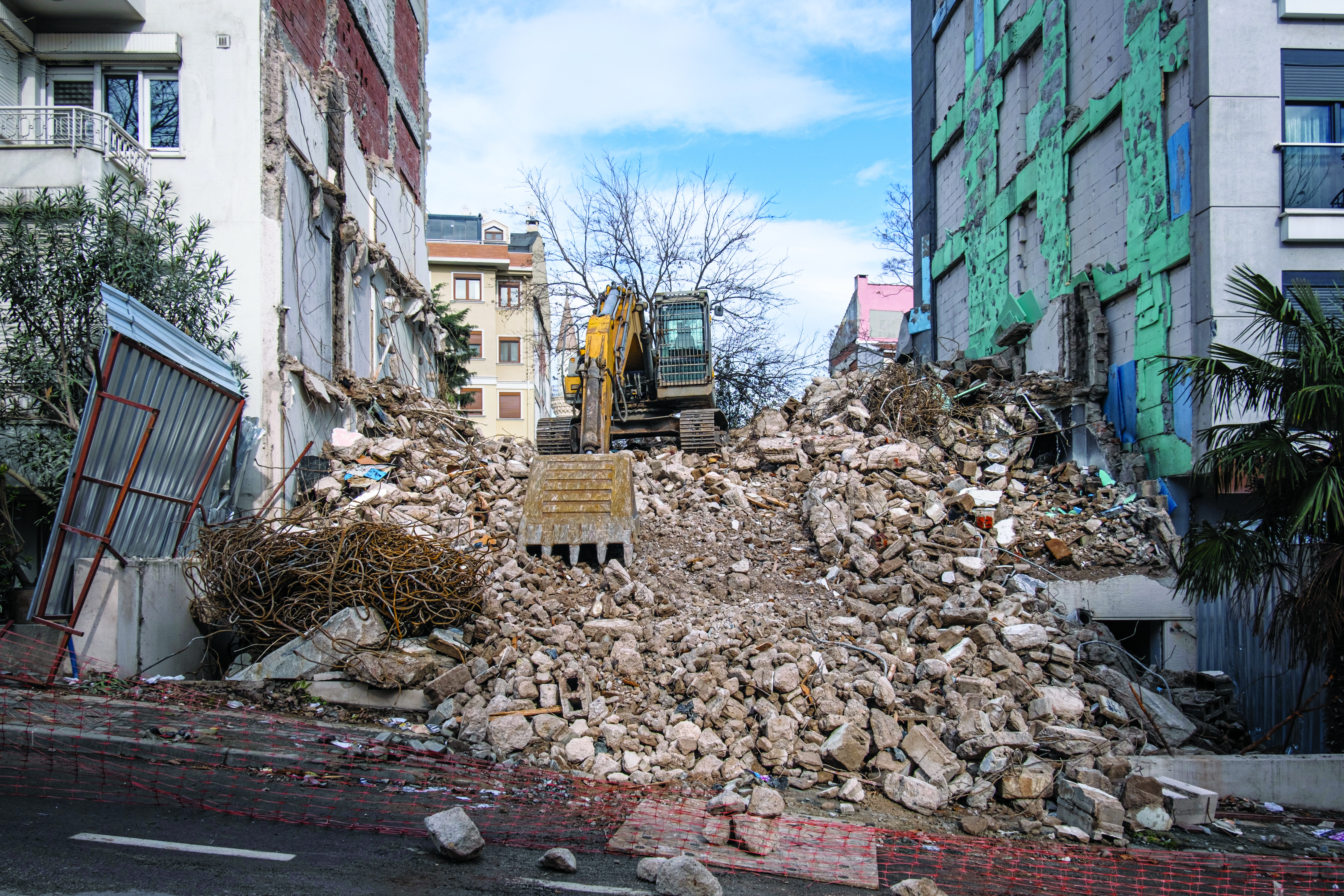
Türkiye is no stranger to earthquakes. In February 2023, a devastating 7.8-magnitude earthquake struck near the Türkiye-Syria border, followed by another nearly as strong.
Six Turkish universities have launched a real-time geodetic monitoring network to track earthquake-related ground deformation across Thrace and the Southern Marmara region, reports Hürriyet Daily News.
TR-TRAK-GNSS will monitor seismic and tectonic activity using 28 GNSS stations. The system is designed to evolve into a major scientific and early-warning infrastructure capable of detecting tectonic deformation in real time and identifying structural movements in buildings across cities and university campuses.
Once fully deployed, the network will form a continuous monitoring ring encircling Thrace and Southern Marmara.
The project will be financed through each participating university’s Scientific Research Projects resources, with institutions covering the installation costs of GNSS stations within their own areas of responsibility.
In my November 2023GPS World newsletter, I highlighted the announcement made by the National Geodetic Survey (NGS) of the recipients of the National Oceanic and Atmospheric Administration (NOAA) FY 2023 Geospatial Modeling Competition Awards. As stated in the newsletter, NGS awarded the grants for projects that will research emerging problems in the field of geodesy and develop tools and models to advance the modernization of the National Spatial Reference System (NSRS). A significant improvement in the new, modernized NSRS is the time-dependent component being incorporated in the computation of reference epoch coordinates (RECs). That said, developing models that accurately capture the time-dependent component is extremely important to providing reliable, consistent, and accurate RECs. This is not a simple problem to solve. Two of the grantees, Scripps Institution of Oceanography (SIO) and The Ohio State University (OSU) include developing models to address what NGS denotes as the Intra-Frame Deformation Model (IFDM).
This newsletter is going to highlight OSU’s geospatial award and my March newsletter will highlight the SIO proposal.
Summary of the OSU Geospatial Awards. (Image: NGS website)
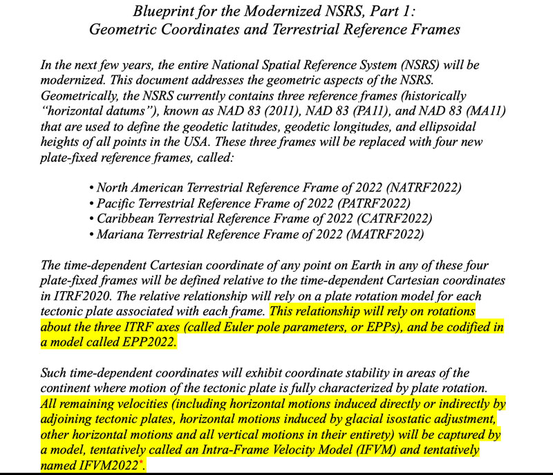
The time-dependent models for the new, modernized NSRS — that is, Euler pole parameters (EPP) and Intra-Frame Deformation Model (IFDM)] — are discussed in NOAA Technical Report NOS NGS 62, “Blueprint for the Modernized NSRS, Part 1: Geometric Coordinates and Terrestrial Reference Frames” and NOAA Technical Report NOS NGS 67, “Blueprint for the Modernized NSRS, Part 3: Working in the Modernized NSRS.” The EPP2022 and IFDM2022 models will make time-dependent geodetic control useable for most surveyors, engineers, and geospatial users.
So, what are EPP2022 and IFDM2022? What does it mean to users of the new, modernized NSRS? Basically, the EPP model changes the reference frame of the coordinates but not the epoch and the IFDM model changes the epoch of the coordinates but not the reference frame.
For the OSU grant proposal, I had the opportunity to talk with Dr. Demián Gómez, the lead principal investigator (PI) for the OSU grant. Demián has extensive experience in modeling time-dependent coordinates and is the lead author on several papers published in the Journal of Geodesy that address this topic.
Articles by Gómez in the Journal of Geodesy
Gómez, D., Piñón, D.A., Smalley, R. et al (2015) Reference frame access under the effects of great earthquakes: a least squares collocation approach for non-secular post-seismic evolution. J Geod. https://doi. org/10. 1007/s00190-015-0871-8
Gómez, D.D., Bevis, M. G. & Caccamise, D.J. Maximizing the consistency between regional and global reference frames utilizing inheritance of seasonal displacement parameters. J Geod 96, 9 (2022). https://doi. org/10. 1007/s00190-022-01594-0
Gómez, D.D., Figueroa, M. A., Sobrero, F. S. et al. On the determination of coseismic deformation models to improve access to geodetic reference frame conventional epochs in low-density GNSS networks. J Geod 97, 46 (2023). https://doi. org/10. 1007/s00190-023-01734-0
In his latest paper, titled “On the determination of coseismic deformation models to improve access to geodetic reference frame conventional epochs in low-density GNSS networks,” the authors applied their methodology to two earthquakes in Chile: the 2010 Maule and 2015 Illapel earthquakes. The paper describes their methodology for estimating coseismic displacements in areas with low-density continuous GNSS coverage by using geophysical models in a hybrid (dynamic-kinematic) mode. Their methodology provided coseismic estimates on survey GNSS stations with rms (95% confidence interval) residuals of ~ 3 cm for Maule, and ~ 2 cm for Illapel. They also tested their models using InSAR and found that the models correctly predicted the near-field deformation. The authors believe that their methodology to obtain coseismic surface displacement models, based on a spherical layered Earth, for GNSS trajectory prediction models (TPMs) using sparse GNSS data represents a major improvement relative to coseismic models incorporated in TPMs, such as NGS’s Horizontal Time-Dependent Positioning model (HTDP) and Transformations in Four Dimensions (TRANS4D). This is important to users of the new, modernized NSRS because the accuracy of the IFDM2022 model is important to providing accurate RECs in the new, modernized NSRS.
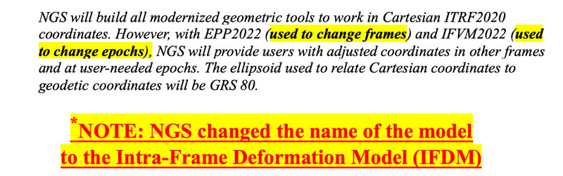
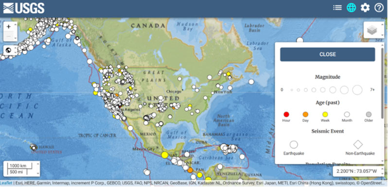
Most individuals in the United States associate earthquakes with California, but earthquakes occur every day in NGS’s area of responsibility. The USGS has a website that lists the location and magnitude of earthquakes.
Plot of earthquakes — 12/21/2023 to 01/20/2024. (Image: USGS website)
The box below highlights the earthquakes in the conterminous United States during a 30-day period. Most of these earthquakes have small magnitudes. The question is, what effects do these earthquakes have on nearby published marks in the NSRS?
Plot of earthquakes in CONUS — 12/21/2023 to 01/20/2024. (Image: USGS website)
The website provides information on both earthquake and non-earthquake events.
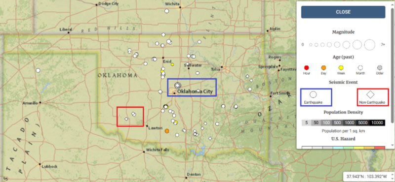
Plot of earthquakes in Oklahoma — 12/21/2023 to 01/20/2024. (Image: USGS website)
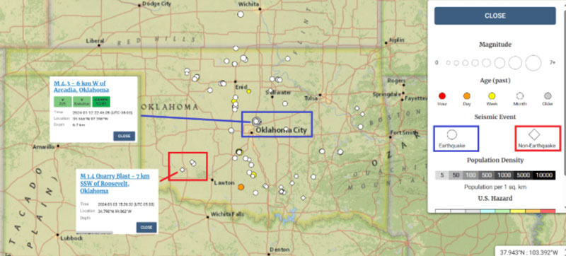
I was wondering what it meant by non-earthquake events, so I clicked on some of the icons. As indicated on the plot, a quarry blast registered on the USGS system. Again, the question is, do these earthquakes and non-earthquake events affect the coordinates of marks in the ground?
Plot of non-earthquakes in Oklahoma. (Image: USGS website)
Something to note in the plots of Oklahoma is the large number of earthquakes around Oklahoma City during a 30-day period.
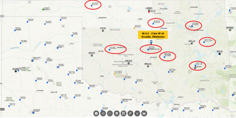
Plot of earthquakes north of Oklahoma City. (Image: USGS website)
Notice that there are several CORSs that surround the location of the earthquakes but only one CORS is close to the area. The box below shows a plot of CORS surrounding the area of earthquakes.
Demián’s latest paper describes their methodology for estimating coseismic displacements in areas with low-density continuous GNSS coverage by using geophysical models in a hybrid (dynamic-kinematic) mode. Since many earthquakes occur throughout the United States, it will be interesting to see how well this approach will work in the development of an Intra-Frame Deformation Model.
Earthquake M 4. 3 – 6 km W of Arcadia, Oklahoma. (Image: NGS website)
As previously stated, outside of California, most of these earthquakes have small magnitudes. That said, on August 9, 2020, a magnitude 5.1 earthquake occurred in Sparta, North Carolina. There were reports of damage to roads, water mains, and structures, but what were the effects on nearby published marks in the NSRS?
Widespread damage occurred in Sparta, which had already been debilitated by the COVID-19 pandemic in North Carolina. [23] Damages include collapsed ceilings, chimneys, and masonry; damaged water mains; cracked and deformed roads; uprooted headstones; and displaced appliances and items. [24][23][25] Wes Brinegar, the town’s mayor, issued a state of emergency to apply for FEMA and state financial aid. [25][23] Damage was worse than initially thought, with at least 525 structures being damaged, and 60 with major damage, meaning at least 40% of the structure was a total loss. Nineteen people lost their homes, 25 were declared uninhabitable, and scammers took advantage of the damage, charging people up to $500 USD for repairs, but never showing up.[26]
Governor of North Carolina, Roy Cooper, toured the damage in Sparta, releasing a statement later, stating “We’ve dealt with a hurricane, a violent tornado, and now an earthquake all in the middle of a pandemic: North Carolinians are resilient.”[27]
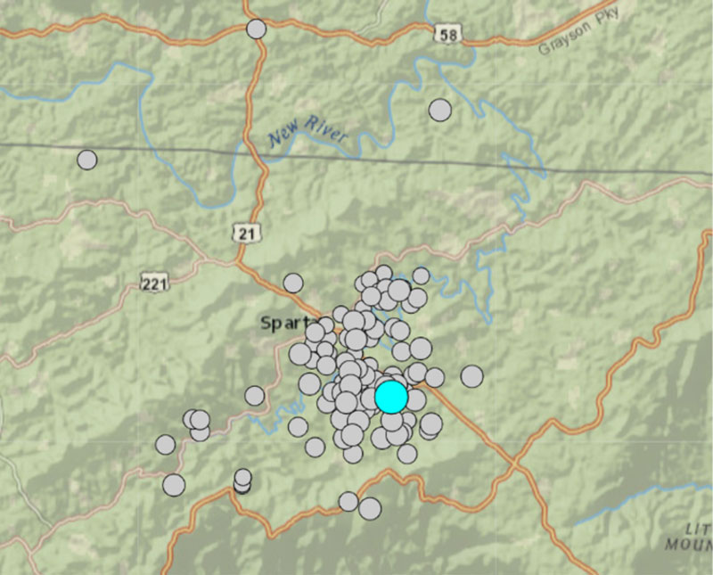
The box below shows the locations of earthquakes that occurred near Sparta, North Carolina. The plot indicates that there was not just one earthquake in the area, but many that may have affected the coordinates of monuments in the region.
Plot of earthquakes near Sparta, North Carolina. (Image: USGS website)
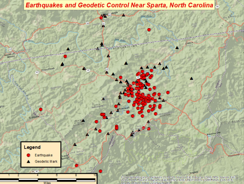
The image below shows the locations of earthquakes and NGS published geodetic marks in the Sparta region.
Image: Dave Zilkoski
Again, the real issue that needs to be addressed is what effect do these earthquakes and other geophysical activities such as subsidence have on the coordinates of geodetic marks in the region?
OSU’s grant proposal includes merging GNSS and InSAR using deep learning to better estimate the Intra-Frame Deformation Model. Obviously, developing time-dependent models for the new, modernized NSRS is very complex and technical. I contacted Demián and asked him for a list of his major milestones associated with his project.
Based on Demián’s major milestones, I had a few follow-up questions.
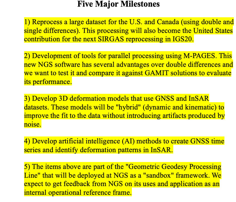
1) Reprocess a large dataset for the U.S. and Canada using double and single differences. This processing will also become the United States’ contribution for the next SIRGAS reprocessing in IGS20.
I asked Demián if he had an estimate of the amount of data he was talking about?
He told me that he did not have an exact number yet because they are still adding data. He said that, at this time, they have 878 stations in the US and Canada which amounts to 4,648,269 station days (i.e., 4. 6M RINEX files, just in the US and Canada). This is the latest number he retrieved from his database but this number increases every day (January 16, 2024).
2) Development of tools for parallel processing using M-PAGES. This new NGS software has several advantages over double differences and we want to test it and compare it against GAMIT solutions to evaluate its performance.
Demián stated that M-PAGES has several advantages so I asked him to explain what he meant.
He told me that one advantage is that it can process all constellations at once using single differences which allows processing of more stations simultaneously. Another advantage is because single differences produce “lighter” systems of equations (compared to double differences), they can process more stations simultaneously.
3) Develop 3D deformation models that use GNSS and InSAR datasets. These models will be “hybrid” (dynamic and kinematic) to improve the fit to the data without introducing artifacts produced by noise.
[Note: this approach is described in the paper titled “On the determination of coseismic deformation models to improve access to geodetic reference frame conventional epochs in low-density GNSS networks,” J Geod 97, 46 (2023).]
Demián said“they are in the process of collecting all the GNSS data that they can to process and then they will identify which gaps can be filled with InSAR data.”
I wanted to better understand what Demián meant by “hybrid” model. So, I asked him about his “hybrid” approach and he provided the following explanation:
When we say “kinematic” we refer to a model that does not consider the underlying mechanism to explain the observed effect. A good example are the trajectory models of GNSS stations that describe their motions as a sum of mathematical functions (there are no physics in them). A dynamic model does use the underlying physics to explain the observations. A “hybrid” model is in the middle: it uses a dynamic model but allows some unrealistic model parameters to improve the data fit.
I mentioned to Demián that users would be very interested in the spatiotemporal uncertainties of the intra-frame deformation model. I asked him if, at this time, he had any idea of the size or range of uncertainties.
Demián said “that it will be variable and very dependent on the density of the input data. He said that they are aiming for cm-level uncertainties. Our experience in Argentina tells us that a 5 mm uncertainty level can be achieved on stable regions while about 2 to 3 cm is expected on high deformation areas. We will have to wait and see to understand the model’s performance. ”
I told Demián that the Houston-Galveston, Texas region of the United States is an area of subsidence that would benefit with an accurate Intra-Frame Deformation Model. The Harris-Galveston Subsidence District has a variety of GNSS CORS and PAMS that are not part of NGS’s CORS. My April 2022 GPS World Newsletter, which included the HGSD CORS and PAMS, described the effects of vertical movement on NGS’s modernized 2022 NSRS. I also asked if he was willing to use this data
He had a very simple answer: “Absolutely!” He said “The more data we incorporate, the better the models will describe reality. Part of the project is related to providing a processing line that can handle large amounts of data. The issue with some data is metadata. Metadata and how we collect it is what really prevents us from reaching that “final mm” uncertainty level we are all looking for. We should be pushing very hard on metadata standardization. In my opinion, the biggest problem is twofold: 1) incorrect antenna identification in RINEX files (due to improper data curation) and 2) lack of a unified/globally accessible database of metadata that is adequately cured.”
4) Develop AI methods to create GNSS time series and identify deformation patterns in InSAR.
Part of the OSU project is to use ML to improve the development of the IFDM.
Excerpt from OSU Proposal on trajectory modeling
Trajectory modeling
For each station, we will obtain KTM parameters, including their uncertainties, for
stations velocities (and acceleration if needed), mechanical and/or geophysical jumps (earthquakes), logarithmic transients after earthquakes (following recommendations from Sobrero et al., 2020), and seasonal coordinate variations. Other parameters for stations affected by volcanic activity, episodic subsidence, etc will also be added when needed. We routinely generate these KTMs for thousands of GNSS stations (for the definition of our in-house geodetic RF) using software developed within the Division of Geodetic Science at OSU. Earthquake detection is performed automatically following formulations also developed by the project’s PIs.
Trajectory modeling enhancement using machine learning
We will enhance the capabilities of the KTMs by including a physics-based machine
learning (ML) component to the model that automatically detects, e. g., discontinuities in the time series. Detecting and mitigating the effects of mechanical jumps (those generated by unreported equipment changes and other effects) will increase the overall reliability of the GGPL. ML is well suited for this task and indeed ML algorithms like Random Forests have been explored in a recent work (e. g., Crocetti et al., 2021). We will test a similar approach, as well as more sophisticated convolutional neural networks to automatically detect discontinuities in coordinate trajectories. These ML algorithms will be trained on OSU’s database of trajectory models (~4000 stations). Using this ML algorithm we will also automatically detect other ‘harmful’ residuals in the time series. For example, large residuals can appear right after an earthquake if the postseismic transient does not have the appropriate relaxation time, or if two transients are needed to model the event.
I find AI and ML fascinating. Basically, machine learning is a field of study in artificial intelligence.
[As a side note: According to Wikipedia, Alan Turing, a mathematician, was the first person to conduct substantial research in the field that he called machine intelligence. Mr. Turing was considered the father of modern computer science. He was famous for his work in decoding the encryption of German Enigma machines during the second world war, and documenting a procedure, known as the Turing Test, that formed the basis for artificial intelligence. Turing was not directly involved with the successful breaking of these more complex codes, but his ideas proved of the greatest importance in this work.]
5) The items above are part of the “Geometric Geodesy Processing Line” that will be deployed at NGS as a “sandbox” framework. We expect to get feedback from NGS on its uses and application as an internal operational reference frame.
The fifth milestone includes developing what Demián calls a “Geometric Geodesy Processing Line (GGPL).” GGPL has three phases, but I am very interested in the first phase. The first phase will begin by analyzing the different components of the GGPL, including the interactions with various geospatial stakeholders, both within and outside of the United States. The plan includes developing a workflow that involves data curation, processing, and analysis to create an operational, fully kinematic reference frame (KRF) for CONUS and Canada. The KRF, once implemented, would at first constitute an experimental or ‘sandbox’ frame executed jointly with NGS’s Geosciences Research Division.
I asked Demián what plans he has for involving users. Especially, how is he going to include surveyors, engineers, photogrammetrists, and spatial data managers?
“My goal is to bring some of the lessons learned in Argentina when we implemented the kinematic reference frame in 2019,” Demián said. Back then, we had discussions with small groups of people in industry to know what their needs were. For example, surveyors will probably need to deal with epoch transformations in a different way than engineers or spatial data managers. The GGPL should facilitate the products that will help these stakeholders. In my experience, the issue is how the data (or model) is accessed so I do not foresee any major issues with users.”
He said that he is open to any suggestions others might have about this.
In phase two, OSU will augment the KRF with locally ‘dynamic’ densifications, which allow
the reference frame to be ‘interpolated’ to locations between the reference stations. Using advanced techniques, such as deep learning, complementary datasets, such as GNSS and InSAR, will be combined and assimilated leading to a kinematic/dynamic reference frame. During phase two, NGS would be assessing the utility and performance of the sandbox GGPL, while OSU works on its dynamic extensions.
In a third phase, the GGPL and the associated KRF and models would undergo any necessary modifications and adaptations, all guided by NGS. By the end of the proposed project, NGS will have a sandbox frame that can implement any new International Terrestrial Reference Frame (ITRF) in a manner that is completely transparent to NSRS users, including all associated models to operate continuously and without interruption.
This newsletter highlighted NGS’s grant to OSU for developing a fully kinematic reference frame for the Continental United States of America and Canada. The primary objectives of this project are to modernize geodetic tools and models and to develop a geodetic workforce for the future. The OSU project will include interactions with various geospatial stakeholders, both within and outside of the United States. In my opinion, it is very important to engage the geospatial user community when developing these new tools so the tools will be useful during the implementation of the new NSRS. A significant improvement in the new, modernized NSRS is the time-dependent component being incorporated in the computation of reference epoch coordinates (RECs). That said, developing models that accurately capture the time-dependent component is extremely important to providing reliable, consistent, and accurate RECs. The goal of the OSU project is to provide an accurate Intra-Frame Deformation Model which will provide reliable, consistent, and accurate reference epoch coordinates (RECs). Throughout the project, OSU would train M.S. and Ph.D. students, and postdocs, providing a source of trained new employees for governmental agencies as well as private industry. Future newsletters will address other NGS recipients of the NOAA FY 23 Geospatial Modeling Competition Awards.
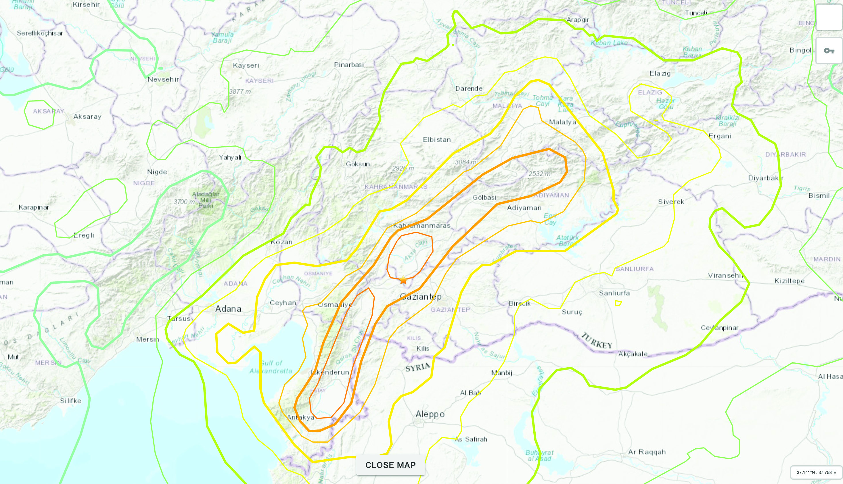
The Mw 7.8 and Mw 7.5 Kahramanmaraş Earthquake Sequence struck near Nurdağı, Türkiye, on Feb. 6. It collapsed several buildings and has claimed more than 50,000 lives. The impact of the initial earthquakes was very severe, but to make matters worse, later in February, a Mw 6.4 tremor struck near Antakya, a city near Türkiye’s border with Syria. This created further damage to infrastructure and claimed more victims.
Image: Screenshot of video from NBC News
The Specifics
The United States Geological Survey reports that the earthquake resulted from strike-slip faulting at shallow depths. The earthquake sequence displaced numerous fault segments within the East Anatolian Fault zone. Early estimates indicate about 185 miles of fault length ruptured. Parts of the North Anatolian Fault shifted 10 feet, while segments of the East Anatolian Fault slid more than 30 feet.
Historic Site Suffers
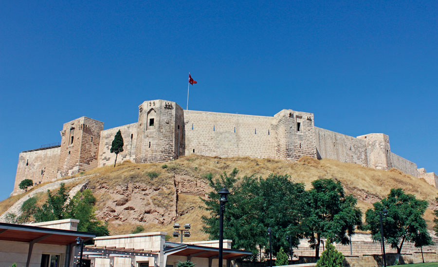
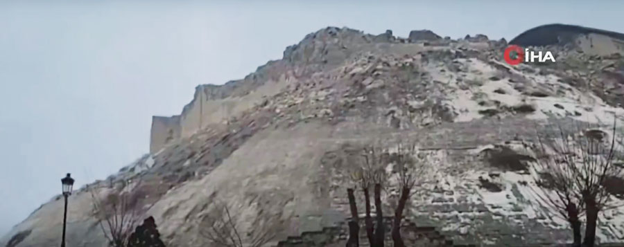
Gaziantep Castle dates back to the second millennium B.C. It has been used in many capacities throughout history, and more recently, stood as a museum for visitors to learn about its rich history. The castle was reduced to rubble in the earthquake. Other historical sites that sustained damage include the Yeni Mosque and the ancient city of Aleppo in Syria.
Image: Screenshot of CNN video
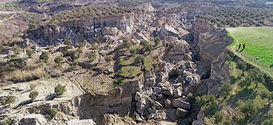
Earth Opens Up
The earthquake destroyed cities all over Türkiye and northern Syria, but they are not the only areas that suffered dramatic effects. A verdant olive grove in Tepehan, Hatay Province, Türkiye, was completely divided when the ground split, creating a 984-foot-long valley in the middle of the grove. The valley is more than 130 feet deep and has created issues for the 7,000 people that inhabit the area.
Previous research suggests that not until halfway through a rupture (90 seconds for a magnitude-9 quake) can magnitude be predicted. Geodetic GNSS data could bring this down to as little as 10 seconds — greatly extending and enhancing earthquake early warning systems.
How soon can we predict the magnitude of an earthquake?
Seismologists Diego Melgar of the University of Oregon and Gavin Hayes of the U.S. Geological Survey (USGS) in Golden, Colorado, tackled this question by chance while Melgar was writing code to simulate earthquakes to check the accuracy of Earthquake Early Warning systems in the Pacific Northwest.
He reached out to Hayes, who curates a database for the USGS that contains “source time functions,” which show how the seismic energy release changes through time as the earthquake ruptures.
As a rupture grows, the speed of growth changes, and source time function captures that change. Melgar and Hayes focused on the acceleration of the energy release in large (M>7) and great (M≥9) earthquakes, and found that acceleration wobbled between 2 and 5 seconds after the quakes began.
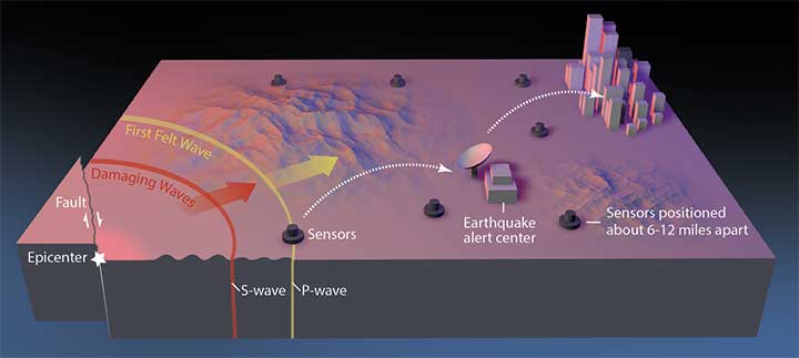
In February 2016, the USGS rolled out the second-generation ShakeAlert Earthquake Early Warning test system in California. The diagram shows how the system would operate. (Image: USGS)
However, with the approximately 250 M≥7 earthquakes in their database, they found that between 10 and 15 seconds after rupture began, these larger earthquakes started to behave similarly, and that behavior scales with their final magnitude, Hayes said. “In other words, the acceleration at 10 to 15 seconds is diagnostic of their final magnitude.”
Earthquake ruptures sputter along for about 10 seconds, after which the big ones accelerate, according to Melgar and Hayes. Three different source time function databases showed the same consistency.
Vertical movement near the source of large earthquakes can be between 3 and 5 meters, according to data from GNSS geodetic receivers. Analysis of near-source GNSS data from 12 M≥7 earthquakes showed that for the first 10 seconds after the first indication of an earthquake was recorded, the earthquakes made almost immeasurable movements. But between 10 and 15 seconds, the amount of vertical displacement began to rapidly diverge for the different magnitude groupings. By 20 to 25 seconds, the vertical movement was distinct.
Previous research indicated roughly half the source duration must pass before an accurate prediction could be made. Cutting the prediction time down to 15 seconds would be invaluable to earthquake early warning systems and tsunami prediction algorithms, where every second counts.
GNSS sensors are installed onshore across the globe, but the majority of megathrust earthquakes occur underwater. To integrate Melgar and Hayes’ findings effectively into earthquake early warning systems would require sensors installed along the seafloor, they noted. “You [would also] need to have fiber-optic cables from shore to the bottom of the ocean, winding around with sensors, and then eventually coming back on shore, and that’s not cheap,” Melgar said.
An additional 10 to 30 seconds of warning to a city or nuclear reactor of an imminent quake would have enormous benefits. But if the hypothesis is wrong, using it now would lead to a greater rate of false alarms and missed quakes, eroding the value of these warnings to society. Melgar and Hayes acknowledged their finding needs to be rigorously tested.
Summarized from Temblor’s website. The Temblor Android app and website provide earthquake, landslide, tsunami and flood information.
Citation
Tripathy-Lang A. (2019), “Can the size of a large earthquake be foretold just 10 seconds after it starts?”. Temblor, http://doi.org/10.32858/temblor.029
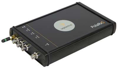
Septentrio has released version 5.1.0 firmware for the PolaRx5 product line of GNSS reference receivers. The 5.1.0 firmware brings new features for file management, usability, security and seismic monitoring.
Septentrio’s PolaRx5 product line of GNSS reference receivers includes the PolaRx5 for CORS and network operations, the PolaRx5TR for time and frequency transfer and the PolaRx5S for space weather applications.
Improvements in precise point positioning (PPP) have opened the door on seismic monitoring using GNSS technology. As well as allowing precise measurement of long-term slow surface displacement, PolaRx5 now allows real-time recording of the high-frequency vibrations typically accompanying earthquakes. Firmware 5.1.0 introduces the support for on-board PPP and dynamic response tuned for seismic applications.
The 5.1.0 firmware release brings greater logging efficiency to the PolaRx5 users. Storage integrity is crucial for many applications. Retransmitting data can be an expensive business, especially when using Iridium telemetry. To improve archival functionality, Septentrio has developed a storage integrity feature to retransmit only the data which has been lost in the initial transmission. This avoids the common and unnecessary overhead of retransmitting complete files.
Preventing unauthorized access is a crucial aspect of cyber security. PolaRx5 product line is now equipped with firewall and IP filtering, SFTP and ssh keys. This complements and strengthens the user management and access level protection of the PolaRx5 product line.
Various independent tests have shown PolaRx5 consistently ranks highest among GNSS receivers in many areas of measurement quality, including lowest measurement noise and fewest number of cycle slips, and this at the lowest power consumption on the market. The PolaRx5 products offer robust and high-quality GNSS tracking of GPS, GLONASS, Galileo and BeiDou as well as regional satellite systems including QZSS and IRNSS.
Some of those who have recently deployed the PolaRx5 include the Oregon Department of Transport (DOT), UNAVCO, the Jet Propulsion Laboratory (JPL) and the SAPOS CORS network in Germany.
“The 5.1.0 PolaRx5 firmware continues Septentrio’s commitment to its customers.” stated Francesca Clemente, PolaRx Product Manager. She continued: “The new features of the 5.1.0 firmware complement existing standard features of the PolaRx5 GNSS receivers such as Advanced Interference Mitigation technology (AIM+) and the web UI offering full user control and status to make PolaRx5 the most complete GNSS reference station on the market today.”
Abstract submissions are now being accepted for The Institute of Navigation’s (ION) Pacific PNT Conference, to be held April 20-23, 2015, at the Waikiki Beach Marriott, Honolulu, Hawaii. Abstracts are due November 14, 2014.
Pacific PNT, where “East Meets West in the Global Cooperative Development of Positioning, Navigation and Timing Technology,” brings together policy and technical leaders from Japan, Singapore, China, South Korea, Australia, the United States, and more for policy updates, program status and technical exchange.
“Global cooperative interoperability” will frame the technical program. Leaders representing academia, government, industry and the scientific community will convene to solve PNT challenges that impact Pacific Rim development.
Pacific PNT 2015 is organized by a Pacific Rim advisory board and will feature technical papers presented on a diverse array of topics including:
Aircraft Navigation and Surveillance
Agricultural, Construction and Mining
Algorithms and Methods
Alternative Navigation and Signals of Opportunity
Aviation Applications of GNSS
Challenging Navigation Problems
Collaborative Navigation Topics
Earthquake & Tsunami Prediction and Monitoring with GNSS
GNSS Augmentations
GNSS Correction and Monitoring Networks
GNSS Environmental Monitoring
GNSS Policy/Status Updates
GNSS Signal Structures
Inertial Navigation Technology and Applications
Interference and Spectrum
Ionosphere Monitoring with GNSS
Magnetic Field Navigation and Mapping
Maritime Navigation
Nature-Inspired Navigation
PNT and Automobile Safety
PNT and Social Media
PNT for Domestic and Healthcare Applications
Precision Agriculture and Machine Control
Time and Frequency Distribution
UAS Technologies
Abstracts are being accepted through November 14, 2014. For more information the ION’s Pacific PNT 2015, visit www.ion.org/pnt.
PTTI 2014 Registration Opens
Registration is now open for the ION Precise Time & Time Interval Meeting (PTTI) 2014 to be held December 1-4 at the Seaport Boston Hotel, Boston, Massachusetts. The technical program is available online.
The annual PTTI conference has a technical program designed to disseminate and coordinate PTTI information at the user level; review present and future PTTI requirements; inform government and industry engineers, technicians, and managers of precise time and frequency technology and its problems; and provide an opportunity for an active exchange of new technology associated with PTTI.
The Distinguished PTTI Service Award, which recognizes outstanding contributions related to the management of PTTI systems, will be presented on Thursday, December 4.
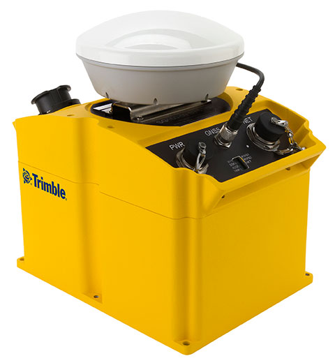
Trimble has introduced an integrated GNSS reference receiver, broadband seismic recorder and a force-balance triaxial accelerometer for infrastructure and precise scientific applications.
The Trimble SG160-09 SeismoGeodetic system provides real-time GNSS positioning and seismic data for earthquake early warning and volcano monitoring as well as infrastructure monitoring for buildings, bridges, dams, as well as other natural and manmade structures.
The Trimble SG160-09 SeismoGeodetic system combines the innovation, reliability and data integrity of both the Trimble and REF TEK brands into a single instrument, Trimble said. The system integrates seismic recording with GNSS geodetic measurement in a single compact, ruggedized package. It includes a low-power, 220-channel GNSS receiver powered by the latest Trimble-precise Maxwell 6 technology and supports tracking of both GPS and GLONASS signals plus the Galileo E1 frequency.
The system includes both the SG160-09 and utilization of Trimble’s CenterPoint RTX correction service, which provides on-board GNSS point positioning. Based on Trimble RTX technology, the service utilizes satellite clock and orbit information delivered over cellular networks or Internet Protocol (IP), allowing cm-level position displacement tracking in real-time anywhere in the world. The SG160-09 system will be available for purchase without the RTX correction service for those applications using real-time kinematic (RTK) positioning.
The seismic recording sensor includes an ANSS Class A, low-noise, force-balance triaxial accelerometer with the latest, low-power, 24-bit A/D converter, which produces high-resolution seismic data. The internally built accelerometer has +/- 4g full scale output, large linear range, high resolution and sensitivity, which makes it ideal for both portable and permanent deployment. The SG160-09 processor acquires and packetizes both seismic and geodetic data and transmits it to system operators using an advanced, error-correction protocol with back-fill capability providing data integrity between the field and the processing center.
The SG160-09 system is ideal for earthquake early warning studies and other hazard mitigation applications, such as volcano monitoring, building, bridge and dam monitoring systems. The SG160-09 system features a variable size industrial grade USB drive to support real-time telemetry data transmission. In the event of a telemetry link outage, the data is stored on the USB drive and can be re-transmitted to the centralized processing station as soon as the communication link comes back up, allowing no data loss during the system operation.
The Trimble SG160-09 system is optimized for field use with instrument mounted or externally mounted GNSS antenna configurations. The lightweight yet rugged SG160-09 consumes very little power and can be used for projects with remote connectivity and in extreme weather conditions. Because the SG160-09 combines both GNSS and strong motion in a single instrument, site installation time is reduced, data communications flow through a single pathway, and station power infrastructure is streamlined, making the SG160-09 a cost competitive solution compared to other systems on the market today. It has an IP67 rating, which means it is sealed against dust and can be submerged in water up to a meter for approximately 30 minutes. The SG160-09 also meets MIL-STD 810F standard for drops, vibration and temperature extremes.
“The SG160-09 is another example of Trimble’s on-going focus in GNSS and seismic technology for the scientific and engineering communities,” said Ulrich Vollath, general manager for Trimble’s Infrastructure Division. “Trimble has developed a combined state-of-the-art GNSS receiver with a high-dynamic range, low-noise accelerometer that provides dynamic monitoring with the flexibility required for today and tomorrow’s challenges.”
The Trimble SG160-09 SeismoGeodetic system is expected to be available in the fourth quarter of 2014.
The explosion of an underground nuclear device by North Korea this week disturbed the Earth’s ionosphere. The blast generated infrasonic waves that propagated all the way to the upper atmosphere causing small variations in the density of electrons there.
By analyzing the signals from GPS satellites collected at ground-based monitoring stations in South Korea and Japan, scientists at the California Institute of Technology’s Jet Propulsion Laboratory, Purdue University, and the Korea Advanced Institute of Science and Technology independently confirmed the ionospheric disturbance generated by the North Korean test.
The researchers used the same GPS signals that are used by surveyors for precise positioning. These signals are slightly perturbed as they transit the ionosphere, and by processing the collected data with sophisticated software, the researchers were able to detect the small effect that the explosion-induced atmospheric waves had on the distribution of the ionosphere’s electrons.
The same technique is being used by the researchers and others to study the ionospheric effects from natural hazards such as tsunamis, earthquakes, and volcanic eruptions.
Using a large network of GPS stations, a team of researchers has found that the Rio Valley Rift in the Southwest United States — previously suspected to be dead — is slowly expanding, at a rate of about 0.1 millimeter per year.
The Rio Grande Rift extends from Colorado’s central Rocky Mountains to Mexico.
The study was conducted by scientists at the Cooperative Institute for Research in the Environmental Sciences (CIRES) at the University of Colorado at Boulder, in collaboration with the University of New Mexico, New Mexico Tech, Utah State University, and UNAVCO.
“We don’t expect to see a lot of earthquakes, or big ones, but we will have some earthquakes,” said study author Anne Sheehan, CIRES Fellow and associate director of CIRES Solid Earth Sciences Division. “We use continuous measurements of GPS sites from across the Rio Grande Rift, Great Plains, and Colorado Plateau to estimate present-day surface velocities and strain rates,” Sheehan said.
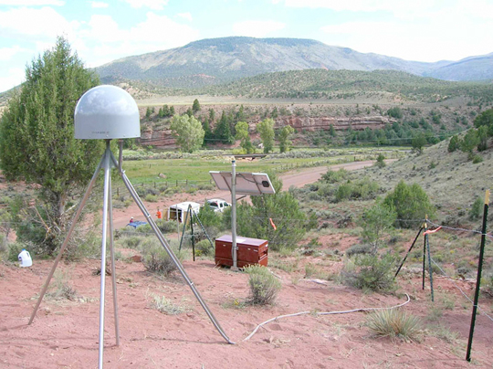
Using GPS instruments at 25 sites in Colorado and New Mexico, the team tracked the rift’s miniscule movements from 2006 to 2011. The team found an average strain rate of 1.2 nanostrain each year across the experimental area. A nanostrain is a change in length of one part per billion, thus 1.2 nanostrain per year is equivalent to 1.2 millimeter per year extension over a 1000-kilometer length.“If you picked two points in New Mexico, and one of them lies 100 kilometers to the west of the other, then they would be moving apart at a rate of 0.1 millimeter per year,” explained researcher Henry Berglund.
Researchers used data from 25 continuous GPS stations installed as part of the EarthScope Rio Grande Rift GPS experiment, supplemented by data from other GPS monuments in the southwestern U.S., resulting in a data set of daily position estimates of 284 GPS monuments for the years 2006 through 2010.
“It is lower than we thought but it does exist,” Sheehan said. “Some people thought it was zero but we are seeing things are extending slowly.”
The slow rates of motion made previous attempts to determine tectonic activity difficult. Previously, geologists had estimated the rift had spread apart by up to 5 millimeters each year but the errors introduced by the measuring instrumentations were significant. “The GPS has reduced the uncertainty dramatically,” Sheehan said. “This is the most comprehensive and accurate set of geodetic measurements in this area to date.”
The extensional deformation is not concentrated in a narrow zone centered on the Rio Grande Rift. Instead, it is distributed broadly from the western edge of the Colorado Plateau into the western Great Plains — a span of more than 370 miles. “This unexpected pattern of broadly distributed deformation at the surface has important implications for our understanding of how low strain-rate deformation within continental interiors is accommodated,” Sheehan said. “Questions we wanted to answer are: how is the Rio Grande Rift deforming? Is it alive or dead? Is it opening or not?”
Along the rift, spreading motion in the crust has caused magma to rise to the surface, creating long basins susceptible to earthquakes. “The rift is still active,” Sheehan said.
The team plans to continue monitoring the Rio Grande Rift, and may attempt to determine vertical as well as horizontal activity to determine whether the Rocky Mountains are still uplifting.
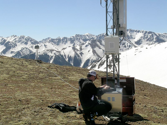
University of Colorado (Boulder) student Henry Berglund services GPS site RG20 west of Silverton, Colorado.
The study’s findings shed light on how continents deform away from plate boundaries, Sheehan said. At plate boundaries scientists can clearly see what is going on. “Things move past each other and crash into each other. At active plate boundaries, the rates of motion detected by GPS can be centimeters per year. Compare that with the fraction of a millimeter per year that we have measured for the Rio Grande Rift.”
“Present day measurements of deformation within continental interiors have been difficult to capture due to the typically slow rates of deformation within them,” Berglund said. “Now, with the recent advances in space geodesy, we are finding some very surprising results in these previously unresolved areas.”
The National Science Foundation funded the study. EarthScope and UNAVCO provided instruments, equipment, and engineering services. Results of the study were published in the January 2012 issue of Geology magazine.
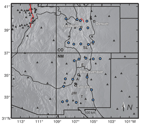
GPS monuments in the vicinity of the Rio Grande Rift and southern Rocky Mountains. The study included construction of 25 GPS monuments (blue circles) in Colorado and New Mexico in 2006 and 2007. Regional EarthScope Plate Boundary Observatory and Continuously Operating Reference Station monuments are shown by gray triangles.
The Earth’s surface is constantly shifting, being deformed as earthquake faults accumulate strain, and slip or slowly creep over time. Not long ago, scientists relied solely on seismometers to monitor the earth’s movements. Today, GPS has taken prominence as an indispensible tool.
PANGA, the monitoring network covering the Pacific Northwest, uses GPS to monitor this movement by measuring the precise position (within 5 millimeters or less) of stations near active faults relative to each other. By determining how the stations have moved, ground deformation can be determined.
If the plates near the coast or the Cascade Mountains move even a few centimeters, the scientists at PANGA know within seconds. The network is still being built, but eventually it’s expected that PANGA will be able to sense earthquakes faster and more accurately than traditional seismometers, and issue alerts to warn citizens of impending activity.
“GPS is helpful in distinguishing magnitude 8 from M9 earthquakes quickly,” explained Rex Flake, PANGA. “By design, seismometers only record high-frequency energy that becomes saturated during strong ground motion. Moreover, seismic data ‘clip’ at high magnitudes whereas GPS become more accurate. Seismographs are mainly intended to detect very small to moderately large earthquakes. GPS gives actual ground motions that in theory could be incorporated very quickly into tsunami models and warning systems. That is one of the things we are working on now.”
Volcano Watch. “A more speculative application is that some (not all by any measure) large earthquakes are preceded by slow creep events,” said Andrew Miner, PANGA. “While not really good enough to predict an earthquake, I think if we saw a very large transient creep event it would at least ring alarm bells. Unfortunately though, earthquakes are by their nature just not very predictable, at least to the level of a day or week that people could reasonably act on. On the bright side, volcanoes are reasonably predictable, and GPS is also an important tool in monitoring them. We work with the Cascade Volcano Observatory on several monitoring projects.”
PANGA is one of a series of earthquake monitoring networks stretching along the West Coast. The Pacific Northwest Geodetic Array is run by the PANGA Geodesy Laboratory at Central Washington University (CWU) in Ellensburg, and includes 300 continuously operating, high-precision GPS receivers located throughout the Pacific Northwest. Sixty more stations are expected to be installed this year. Trimble, Leica, Topcon, and Javad are the main receivers used in the region.
Data from these receivers is continuously downloaded, analyzed, archived, and disseminated. About one third of PANGA’s GPS stations are telemetered in real-time back to CWU, where the data are processed using NASA’s Jet Propulsion Laboratory’s GIPSY/OASIS II software for high-precision data analysis, and Trimble’s RTKNet Integrity Manager software for real-time analysis. The data provide relative positioning of several millimeters across the Cascadia subduction zone and its metropolitan regions. These real-time data are used to monitor and mitigate natural hazards arising from earthquakes, volcanic eruptions, landslides, and coastal sea-level hazards.
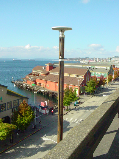
Sagging Bridges. The data are also used to monitor man-made structures such as Seattle’s sagging Alaska Way Viaduct, the State Route 520 and Interstate 90 floating bridges, and dams throughout the Cascadia subduction zone, including those along the Columbia River. For instance, for the S.R. 520 bridge, PANGA teamed up with Washington State Department of Transportation (WSDOT) to monitor movement of the 520 bridges during wind storms and seismic events.
The receivers continuously monitor and record structural deformation with about a millimeter precision. Raw GNSS satellite phase and pseudorange estimates are acquired and processed continuously into receiver positions estimated every 5 seconds and delivered with 10 and 30-second latencies. Daily-averaged receiver positions computed with predicted and post-processed satellite orbit and clock corrections are provided with 1-6 day latencies.
Seattle’s aging Alaska Way viaduct is one of several major man-made structures being monitored by PANGA’s GPS Network. (photos courtesty of CWU Geodesy Lab.)
Tremor Slips. The Northwest is at the forefront of earthquake-related GPS research, in large part because the area provides a lot to learn from GPS monitoring, Flake said. “For example, when we started it was strongly suspected but not definitely known that the Cascadia subduction zone was locked over parts of its surface and a major earthquake threat. Thanks to GPS monitoring we now have a pretty good idea not only exactly where it is locked, but also when parts of it do slip or creep.
“One important discovery made with GPS data, along this line, was that of the Episodic Tremor Slip (ETS) events that occur here in the Northwest U.S.,” Flake said. “Since the time duration of ETS motion takes place on the scale of days to weeks, these earthquake events were unrealized by traditional seismic detection methods.”
GPS data shed light on this peculiarly predictable earthquake phenomenon. “With these GPS data we can measure strain accumulation within the continental crust (where people live) and calculate the residual that can be expected to rebound in a large subduction zone earthquake,” Flake said.
“Even more detailed than that, we can use GPS data from past ETS events to constrain the locked zone of the subducting crustal plate by inferring the amount of slip at depth that best reproduces the observed GPS recordings — important in determining possible magnitude and location of the megathrust earthquakes (Mw = 8 to 9) that will someday occur. This is of obvious concern to society and is a major reason that we lead the geodetic applications of GPS research.”
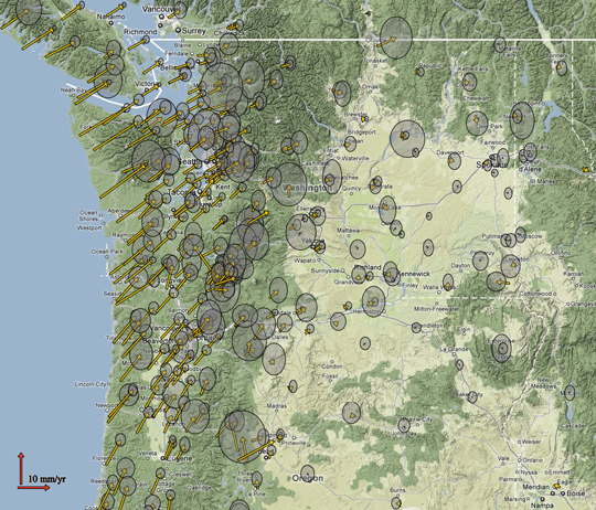
Data Online. PANGA maintains a website that integrates daily GPS measurements from about 1,500 stations along the Pacific/North American plate boundary, ranging from Alaska to the U.S-Mexico border. Cleaned, network solutions from several arrays are merged and grouped into regional clusters.
Arrow on a Velocity Field Map of Oregon and Washington represent ground motion as measured by GPS at each particular location. The grey circles are 2 sigma error ellipses (click to enlarge.) (photos courtesty of CWU Geodesy Lab.)
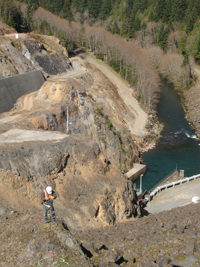
The PANGA team constructs a bedrock drill-brace geodetic monument at Howard Hanson Dam east of Auburn, Washington. (photos courtesty of CWU Geodesy Lab.)
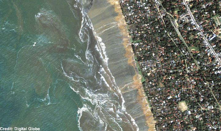
QuickBird satellite image of Kalutara Beach on the southwestern coast of Sri Lanka showing the receding waters and beach damage from the Sumatra tsunami.( Credit: Digital Globe)
How Ionospheric Observations Might Improve the Global Warning System
By Giovanni Occhipinti, Attila Komjathy, and Philippe Lognonné
Recent investigations have demonstrated that GPS might be an effective tool for improving the tsumani early-warning system through rapid determination of earthquake magnitude using data from GPS networks. A less obvious approach is to use the GPS data to look for the tsunami signature in the ionosphere.
INNOVATION INSIGHTS by Richard Langley
THE TSUNAMI generated by the December 26, 2004, earthquake just off the coast of the Indonesian island of Sumatra killed over 200,000 people. It was one of the worst natural disasters in recorded history. But it might have been largely averted if an adequate warning system had been in place.
A tsunami is generated when a large oceanic earthquake causes a rapid displacement of the ocean floor. The resulting ocean oscillations or waves, while only on the order of a few centimeters to tens of centimeters in the open ocean, can grow to be many meters even tens of meters when they reach shallow coastal areas. The speed of propagation of tsunami waves is slow enough, at about 600 to 700 kilometers per hour, that if they can be detected in the open ocean, there would be enough time to warn coastal communities of the approaching waves, giving people time to flee to higher ground.
Seismic instruments and models are used to predict a possible tsunami following an earthquake and ocean buoys and pressure sensors on the ocean bottom are used to detect the passage of tsunami waves. But globally, the density of such instrumentation is quite low and, coupled with the time lag needed to process the data to confirm a tsunami, an effective global tsunami warning system is not yet in place.
However, recent investigations have demonstrated that GPS might be a very effective tool for improving the warning system. This can be done, for example, through rapid determination of earthquake magnitude using data from existing GPS networks. And, incredible as it might seem, another approach is to use the GPS data to look for the tsunami signature in the ionosphere: the small displacement of the ocean surface displaces the atmosphere and makes it all the way to the ionosphere, causing measurable changes in ionospheric electron density.
In this month’s column, we look in detail at how a tsunami can affect the ionosphere and how GPS measurements of the effect might be used to improve the global tsunami warning system.
“Innovation” is a regular column that features discussions about recent advances in GPS technology and its applications as well as the fundamentals of GPS positioning. The column is coordinated by Richard Langley of the Department of Geodesy and Geomatics Engineering at the University of New Brunswick.
The December 26, 2004, earthquake-generated Sumatra tsunami caused enormous losses in life and property, even in locations relatively far away from the epicentral area. The losses would likely have never been so massive had an effective worldwide tsunami warning system been in place. A tsunami travels relatively slowly and it takes several hours for one to cross the Indian Ocean, for example. So a warning system should be able to detect a tsunami and provide an alert to coastal areas in its path. Among the strengths of a tsunami early-warning system would be its capability to provide an estimate of the magnitude and location of an earthquake. It should also confirm the amplitude of any associated tsunami, due to massive displacement of the ocean bottom, before it reaches populated areas. In the aftermath of the Sumatra tsunami, an important effort is underway to interconnect seismic networks and to provide early alarms quantifying the level of tsunami risk within 15 minutes of an earthquake.
However, the seismic estimation process cannot quantify the exact amplitude of a tsunami, and so the second step, that of tsunami confirmation, is still a challenge. The earthquake fault mechanism at the epicenter cannot fully explain the initiation of a tsunami as it is only approximated by the estimated seismic source. The fault slip is not transmitted linearly at the ocean bottom due to various factors including the effect of the bathymetry, the fault depth, and the local lithospheric properties as well as possible submarine landslides associated with the earthquake.
In the open ocean, detecting, characterizing, and imaging tsunami waves is still a challenge. The offshore vertical tsunami displacement (on the order of a few centimeters up to half a meter in the case of the Sumatra tsunami) is hidden in the natural ocean wave fluctuations, which can be several meters or more. In addition, the number of offshore instruments capable of tsunami measurements, such as tide gauges and buoys, is very limited. For example, there are only about 70 buoys in the whole world. As a tsunami propagates with a typical speed of 600–700 kilometers per hour, a 15-minute confirmation system would require a worldwide buoy network with a 150-kilometer spacing.
Satellite altimetry has recently proved capable of measuring the sea surface variation in the case of large tsunamis, including the December 2004 Sumatra event. However, satellites only supply a few snapshots along the sub-satellite tracks. Optical imaging of the shore hs successfully measured the wave arrival at the coastline (see ABOVE PHOTO), but it is ineffective in the open sea. At present, only ocean-bottom sensors and GPS buoy receivers supply measures of mid-ocean vertical displacement. In many cases, the tsunami can only be identified several hours after the seismic event due to the poor distribution of sensors. This delay is necessary for the tsunami to reach the buoys and for the signal to be recorded for a minimum of one wave period (a typical tsunami wave period is between 10 and 40 minutes) to be adequately filtered by removing the “noise” due to normal wave action.
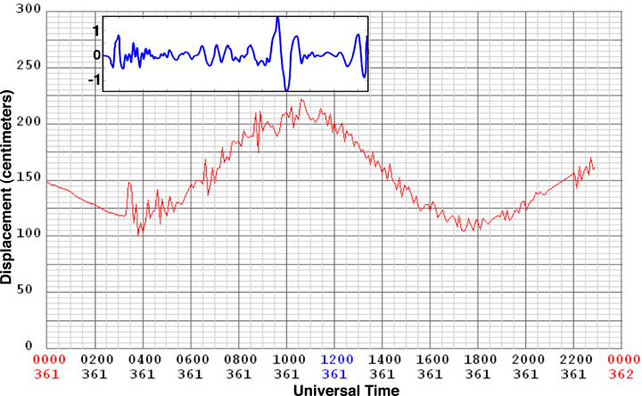
In the case of the December 2004 Sumatra event, the first tsunami measurements by any instrumentation were only made available about 3 hours after the earthquake. They were supplied by the real-time tide gauge at the Cocos Islands, an Australian territory in the southeast Indian Ocean (see FIGURE 1 where the tsunami signature is superimposed on the large semidiurnal tide fluctuation). Up until that time, the tsunami could not be fully confirmed and coastal areas remained vulnerable to tsunami damage. This delay in confirmation is a fundamental weakness of the existing tsunami warning systems.
Figure 1. The Sumatra tsunami signal measured at the Cocos Islands by the tide gauge (red) and by the co-located GPS receiver (blue). The tide gauge measures the sea-level displacement (tide plus superimposed tsunami) and the GPS receiver measures the slant total electron content perturbation (+/-1 TEC unit) in the ionosphere.
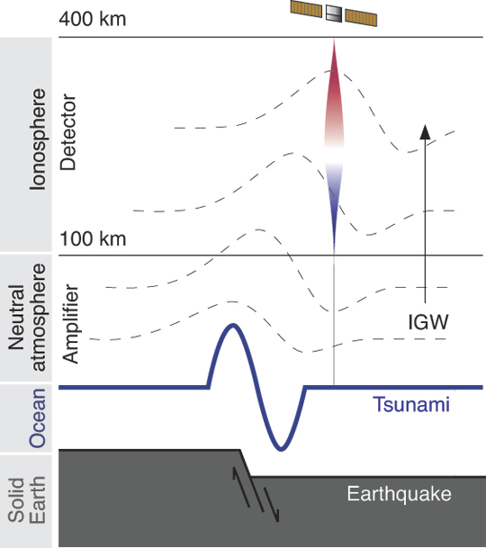
Ionospheric Perturbation. Recently, observational and modeling results have confirmed the existence and detectability of a tsunamigenic signature in the ionosphere. Physically, the displacement induced by tsunamis at the sea surface is transmitted into the atmosphere where it produces internal gravity waves (IGWs) propagating upward. (When a fluid or gas parcel is displaced at an interface, or internally, to a region with a different density, gravity restores the parcel toward equilibrium resulting in an oscillation about the equilibrium state; hence the term gravity wave.) The normal ocean surface variability has a typical high frequency (compared to tsunami waves) and does not transfer detectable energy into the atmosphere. In other words, the Earth’s atmosphere behaves as an “analog low-pass filter.” Only a tsunami produces propagating waves in the atmosphere. During the upward propagation, these waves are strongly amplified by the double effects of the conservation of kinetic energy and the decrease of atmospheric density resulting in a local displacement of several tens of meters per second at 300 kilometers altitude in the atmosphere. This displacement can reach a few hundred meters per second for the largest events.
At an altitude of about 300 kilometers, the neutral atmosphere is strongly coupled with the ionospheric plasma producing perturbations in the electron density. These perturbations are visible in GPS and satellite altimeter data since those signals have to transit the ionosphere. The dual-frequency signal emitted by GPS satellites can be processed to obtain the integral of electron density along the paths between the satellites and the receiver, the total electron content (TEC).
Within about 15 minutes, the waves generated at the sea surface reach ionospheric altitudes, creating measurable fluctuations in the ionospheric plasma and consequently in the TEC. This indirect method of tsunami detection should be helpful in ocean monitoring, allowing us to follow an oceanic wave from its generation to its propagation in the open ocean.
So, can ionospheric sounding provide a robust method of tsunami confirmation? It is our hope that in the future this technique can be incorporated into a tsunami early-warning system and complement the more traditional methods of detection including tide gauges and ocean buoys. Our research focuses on whether ground-based GPS TEC measurements combined with a numerical model of the tsunami-ionosphere coupling could be used to detect tsunamis robustly. Such a detection scheme depends on how the ionospheric signature is related to the amplitude of the sea surface displacement resulting from a tsunami. In the near future, the ionospheric monitoring of TEC perturbations might become an integral part of a tsunami warning system that could potentially make it much more effective due to the significantly increased area of coverage and timeliness of confirmation.
In this article, we’ll take a look at the current state of the art in modeling tsunami-generated ionospheric perturbations and the status of attempts to monitor those perturbations using GPS.
Some Background
Pioneering work by the Canadian atmospheric physicist Colin Hines in the 1970s suggested that tsunami-related IGWs in the atmosphere over the oceanic regions, while interacting with the ionospheric plasma, might produce signatures detectable by radio sounding.
In June 2001, an episodic perturbation was observed following a tsunamigenic earthquake in Peru. After its propagation across the Pacific Ocean (taking about 22 hours), the tsunami reached the Japanese coast and its signature in the ionosphere was detected by the Japanese GPS dense network (GEONET). The perturbation, shown in FIGURE 2, has an arrival time and characteristic period consistent with the tsunami propagation determined from independent methods. Unfortunately, similar signatures in the ionosphere are also produced by IGWs associated with traveling ionospheric disturbances (TIDs), and are commonly observed in the TEC data. However, the known azimuth, arrival time, and structure of the tsunami allows us to use this data source, even if it contains background TIDs.
Figure 2. The observed signal for the June 23, 2001, tsunami (initiated offshore Peru). Total electron content variations are plotted at the ionosphere pierce points. A wave-like disturbance is seen propagating toward the coast of Honshu, the main island of Japan.
The December 26, 2004, Sumatra earthquake, with a magnitude of 9.3, was an order of magnitude larger than the Peru event and was the first earthquake and tsunami of magnitude larger than 9 of the so-called “human digital era,” comparable to the magnitude 9.5 Chilean earthquake of May 22, 1960.
In addition to seismic waves registered by global seismic networks, the Sumatra event produced infragravity waves (long-period wave motions with typical periods of 50 to 200 seconds) remotely observed from the island of Diego Garcia, perturbations in the magnetic field observed by the CHAMP satellite, and a series of ionospheric anomalies.
Two types of ionospheric anomaly were observed: anomalies of the first type, detected worldwide in the first few hours after the earthquake, were reported from north of Sumatra, in Europe, and in Japan. They are associated with the surface seismic waves that propagate around the world after an earthquake rupture (so-called Rayleigh waves).
Anomalies of the second type were detected above the ocean and were clearly associated with the tsunami. In the Indian Ocean, the occurrence times of TEC perturbations observed using ground-based GPS receivers and satellite altimeters were consistent with the observed tsunami propagation speed. The GPS observations from sites to the north of Sumatra show internal gravity waves most likely coupled with the tsunami or generated at the source and propagating independently in the atmosphere. The link with the tsunami is more evident in the observations elsewhere in the Indian Ocean. The TEC perturbations observed by the other ground-based GPS receivers moved horizontally with a velocity coherent with the tsunami propagation.
Figure 3. The tsunamigenic earthquake mechanism and transfer of energy in the neutral and ionized atmosphere. The solid Earth displacement produces the tsunami and the sea surface displacement produces an internal gravity wave in the neutral atmosphere, which perturbs the electron distribution in the ionosphere.
The amplitude of the observed TEC perturbations is strongly dependent on the filter method used. The four TECU-level peak-to-peak variations in filtered GPS TEC measurements from north of Sumatra are coherent with the differential TEC at the 0.4 TECU per 30 seconds level observed in the rest of the Indian Ocean. (One TEC unit or TECU is 1016 electrons per meter-squared, equivalent to 0.162 meters of range delay at the GPS L1 frequency.) Such magnitudes can be detected using GPS measurements since GPS phase observables are sensitive to TEC fluctuations at the 0.01 TECU level. We emphasize also the role of the elevation angle in the detection of tsunamigenic perturbations in the ionosphere. As a consequence of the integrated nature of TEC and the vertical structure of the tsunamigenic perturbation, low-elevation angle geometry is more sensitive to the tsunami signature in the GPS data, hence it is more visible.
The TEC perturbation observed at the Cocos Islands by GPS can be compared with the co-located tide-gauge (Figure 1). The tsunami signature in the data from the two different instruments shows a similar waveform, confirming the sensitivity of the ionospheric measurement to the tsunami structure.
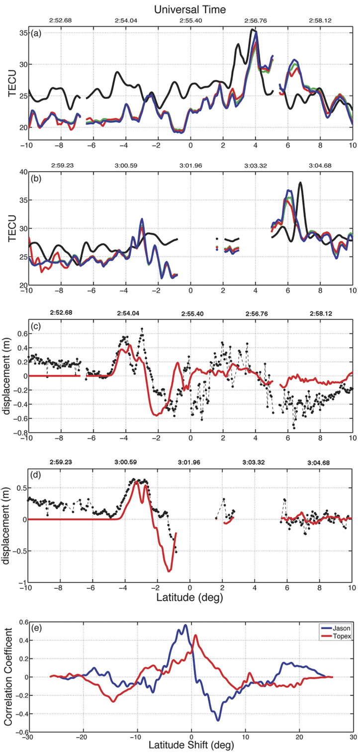
The link between the tsunami at sea level and the perturbation observed in the ionosphere has been demonstrated using a 3D numerical modeling based on the coupling between the ocean surface, the neutral atmosphere, and the ionosphere (see FIGURE 3). The modeling reproduced the TEC data with good agreement in amplitude as well as in the waveform shape, and quantified it by a cross-correlation (see FIGURE 4). The resulting shift of +/-1 degree showed the presence of zonal and meridional winds neglected in the modeling. The presence of the wind can, indeed, introduce a shift of 1 degree in latitude and 1.5 degrees in longitude.
Since modeling is an effective method to discriminate between the tsunami signature in the ionosphere and other potential perturbations, the GPS observations can be a useful tool to develop an inexpensive tsunami detection system based on the ionospheric sounding.
Figure 4. Satellite altimeter and total electron content (TEC) signatures of the Sumatra tsunami. The modeled and observed TEC is shown for (a) Jason-1 and for (b) Topex/Poseidon: data (black), synthetic TEC without production-recombination-diffusion effects (blue), with production-recombination (red), and production-recombination-diffusion (green). The Topex/Poseidon synthetic TEC has been shifted up by 2 TEC units. In (c) and (d), the altimetric measurements of the ocean surface (black) are plotted for the Jason-1 and Topex/Poseidon satellites, respectively. The synthetic ocean displacement, used as the source of internal gravity waves in the neutral atmosphere, is shown in red. In (e), the cross-correlations between TEC synthetics and data are shown for Jason-1 (blue) and Topex/Poseidon (red).
Modeling TEC Perturbations
A model to describe the effect of a tsunami on the ionosphere has been developed at the Institut de Physique du Globe de Paris (IPGP), France. It is comprised of three main parts. Firstly, it computes tsunami propagation using realistic bathymetry of, for example, the Indian Ocean. Secondly, an oceanic displacement is used to excite IGWs in the neutral atmosphere. Thirdly, it computes the response of the ionosphere induced by the neutral atmospheric motion resulting in enhanced electron densities. After integrating the electron densities, we obtain modeled (synthetic) TEC data. The modeling steps are as follows:
Tsunami Propagation. Tsunami modeling is an established science and the propagation of tsunamis is generally based on a shallow-water hypothesis. Under this hypothesis, the ocean is considered as a simple layer where the ocean depth, h, is locally taken into account in the tsunami propagation velocity, v = √ hg, which directly depends on h and the gravity acceleration g. The modeling, usually based on finite differences, solves the appropriate hydrodynamic equations.
Neutral Atmosphere Coupling. A tsunami is an oceanic gravity wave and its propagation is not limited to the oceanic surface; as previously discussed, the ocean displacement is transferred to the atmosphere where it becomes an internal gravity wave. This coupling phenomenon is linear and can be reproduced solving the wave propagation equations, nominally the continuity and the so-called Navier-Stokes equations. These equations are solved assuming the atmosphere to be irrotational, inviscid, and incompressible. The IGWs are, indeed, imposed by displacement of the mass under the effect of the gravity force, contrary to the elastic waves generated by compression (for example, sound waves), so the medium can be considered incompressible. FIGURE 5 shows the IGWs produced by the Sumatra tsunami. The inversion of the velocity with altitude (wind shear) is a typical structure of IGWs.
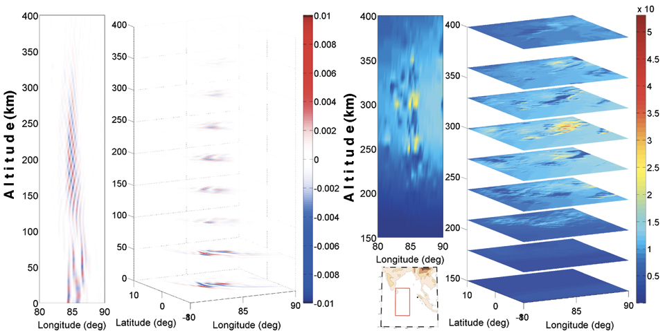
Neutral-Plasma Coupling. The tsunamigenic IGWs are injected into a 3D ionospheric model to reproduce the induced electron density perturbations. In essence, the coupling model solves the hydromagnetic equations for three ion species (O2 + , NO+ , and O+ ). Physically, the neutral atmosphere motion induces fluctuations in the plasma velocity by way of momentum transfer driven by collision frequency and the Lorentz term associated with Earth’s magnetic and electric fields. Ion loss, recombination, and diffusion are also taken into account in the ion continuity equation. Finally, the perturbed electron density is inferred from ion densities using the charge neutrality hypothesis. The International Reference Ionosphere model is used for background electron density; SAMI2 (a recursive acronym: SAMI2 is Another Model of the Ionosphere) is used for collision, production, and loss parameters; and a constant geomagnetic field is assumed based on the International Geomagnetic Reference Field. FIGURE 5 shows the perturbation induced in the ionospheric plasma by the tsunamigenic IGW following the Sumatra event. The perturbation is strongly localized to around 300 kilometers altitude where the electron density background is maximized.
Figure 5. Internal gravity waves (IGWs) generated by the Sumatra tsunami and the response of the ionosphere to neutral motion at 02:40 UT (almost two hours after the earthquake). On the left, the normalized vertical velocity induced by tsunami-generated IGWs in the neutral atmosphere is shown. On the right, the perturbation induced by IGWs in the ionospheric plasma (in electrons per cubic meter) is shown, with the maximum perturbation at an altitude of about 300 kilometers. The vertical cut shown in these profiles is at a latitude of -1 degree.
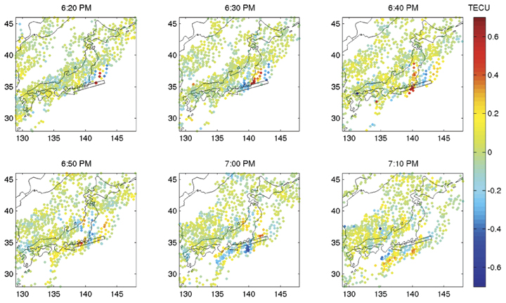
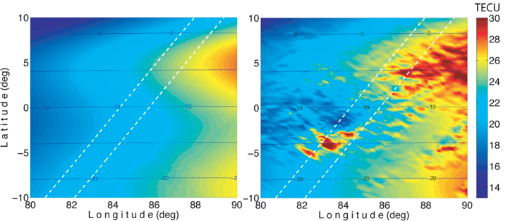
The resulting electron density dynamic model described above allows us to compute a map of the perturbed TEC by simple vertical integration (see FIGURE 6). In addition to the geometrical dispersion of the tsunami, the TEC map shows horizontal heterogeneities in the electron density perturbation that are induced by the geomagnetic field inclination. The magnetic field plays a fundamental role in the neutral-plasma coupling, resulting in a strong amplification at the magnetic equator where the magnetic field is directed horizontally. The isolated perturbation appearing more to the south is probably induced by the full development of the IGW in the atmosphere. Recent work also explains this second perturbation as induced by the role of the magnetic field in the neutral-plasma coupling.
Figure 6. The signature of the Sumatra tsunami in total electron content (TEC) at 03:18 UT (right) compared with the unperturbed TEC (left). The TEC images have been computed by vertical integration of the perturbed and unperturbed electron density fields. The broken lines represent the Topex/Poseidon (left) and Jason-1 (right) trajectories. The blue contours represent the geomagnetic field inclination.
GPS Data Processing
To validate our model, we use ground-based GPS receivers to look for the ionospheric signal induced by tsunamis. Prior research has shown post-processed results detecting a tsunami-generated TEC signal using regional GPS networks such as GEONET in Japan (about 1,000 stations) or the Southern California Integrated GPS Network (about 200 stations). Those studies benefited from the very high density of GPS receivers in the regional networks, so that, for example, no forward modeling was needed to help initially identify the characteristics of the tsunami-generated signal.
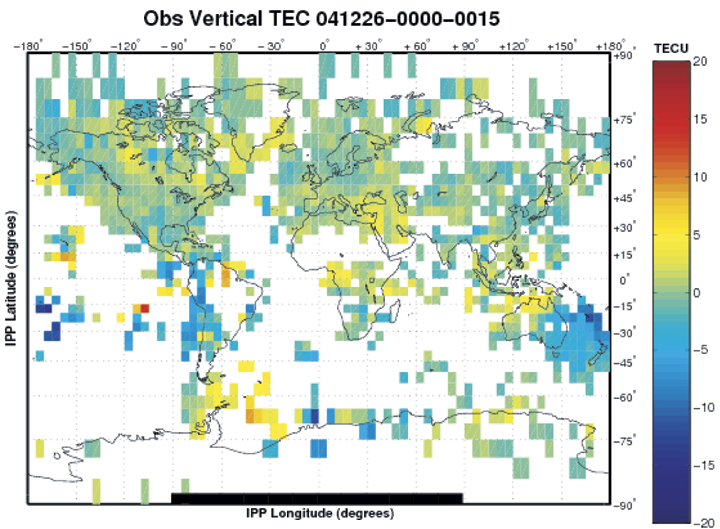
High-Precision Processing. More than 1,300 globally-distributed dual-frequency GPS receivers are available using publicly accessible networks, including those of the International GNSS Service and the Continuously Operating GPS Stations coordinated by the U.S. National Geodetic Survey. Most researchers estimate vertical ionospheric structure and, simultaneously, treat hardware-related biases as nuisance parameters. In our approach for calibrating GPS receiver and satellite inter-frequency biases, we take advantage of all available GPS receivers using a new processing technique based on the Global Ionospheric Mapping software developed at the Jet Propulsion Laboratory (JPL). FIGURE 7 shows a JPL TEC map using 1,000 GPS stations. This new capability is designed to estimate receiver biases for all stations in the global network. We solve for the instrumental biases by modeling the ionospheric delay and removing it from the observation.
Figure 7. The total electron content (TEC) between 01:00 and 01:15 UT on December 26, 2004, at ionosphere pierce points (IPPs) provided by a global network of more than 1,000 GPS tracking stations. To highlight variations, a five-day average of TEC has been subtracted from the observed TEC.
Ionospheric Warning System
The currently implemented tsunami warning system uses seismometers to detect earthquakes and to perform an estimation of the seismic moment by monitoring seismic waves. After a potential tsunami risk is determined, ocean buoy and pressure sensors have to confirm the tsunami risk. Unfortunately, the number of available ocean buoys is limited to about 70 over the whole planet. With the existing system, it may take several hours to confirm a tsunami when taking into account both the propagation time (of tsunamis reaching buoys) and data-processing time. On the other hand, the proposed ionosphere-based tsunami detection system may only require the propagation time and data-processing delays of only up to about 15–30 minutes. GPS receivers are able to sound the ionosphere up to about 20 degrees away from the receiver location, and a dense GPS network can therefore increase the coverage of the monitored area.
The fundamental idea behind a detection method is that we need to separate tsunami-generated TEC signatures from other sources of ionospheric disturbances. However, the tsunami-generated TEC perturbations are distinguishable because they are tied to the propagation characteristics of the tsunami. Tsunami-related fluctuations should be in the gravity-wave period domain and cohere in geometry and distance with the earthquake epicenter (for example, they show up in data on multiple satellites from multiple stations and, with increasing distance from the epicenter, at a rate related to tsunami propagation speed).
The coupled tsunami model described earlier can also be used to compute a prediction for the tsunami-generated TEC perturbation based on the seismic displacement as an input parameter to the model. The model prediction may be used as a detection aid by indicating the location of the tsunami wave front with time. This permits us to focus our detection efforts on specific locations and times, and will allow us to discriminate signal from noise.
The model also provides information on the expected magnitude of the TEC perturbation. This provides further value in filter discrimination. Cross-correlations can be performed on nearby observations using different satellites and stations to take advantage of tsunami-related perturbations being coherent in geometry and distance from the epicenter. Once the signal is detected in data from multiple satellites and stations, we can “track” and image the tsunami during its propagation in space and time.
The goal of our research is to assess the feasibility of detecting tsunamis in near real time. This requires that GPS data be acquired rapidly. Rapid availability of ground-based GPS data has been demonstrated via the NASA Global Differential GPS System, a highly accurate, robust real-time GPS monitoring and augmentation system.
Conclusions
Earlier research using GPS-derived TEC observations has revealed TEC perturbations induced by tsunamis. However, in our research, we use a combination of a coupled ionosphere-atmosphere-tsunami model with large GPS data sets. Ground-based GPS data are used to distinguish tsunami-generated TEC perturbations from background fluctuations. Tsunamis are among the most disrupting forces humankind faces. The December 26, 2004, earthquake and resulting tsunami claimed more than 200,000 lives, with several hundreds of thousands of people injured. The damage in infrastructure and other economic losses were estimated to be in the range of tens of billions of dollars. To help prevent such a global disaster from occurring again, we suggest that ionospheric sounding by GPS be integrated into the existing tsunami warning system as soon as possible.
Acknowledgments
This article is based on the paper “Three-Dimensional Waveform Modeling of Ionospheric Signature Induced by the 2004 Sumatra Tsunami” published in Geophysical Research Letters. The authors wish to acknowledge François Crespon (Noveltis, Ramonville-Saint-Agne, France) for the TEC data analysis in Figure 1, Juliette Artru (Centre National d’Etudes spatiales – CNES, Toulouse, France) for her work on the detection of tsunamigenic TEC perturbations shown in this article, and Grégoire Talon for Figure 3. The IPGP portion of the work is sponsored by L’Agence Nationale de la Recherche, by CNES, and by the Ministère de l’Enseignement supérieur et de la Recherche. The first author would also like to thank John LaBrecque of NASA’s Science Mission Directorate for supporting his fellowship at the California Institute of Technology/JPL.
GIOVANNI OCCHIPINTI received his Ph.D. at the Institut de Physique du Globe de Paris (IPGP) in 2006. In 2007, he joined NASA’s Jet Propulsion Laboratory (JPL), California Institute of Technology, as a postdoctoral fellow to continue his work on the detection and modeling of tsunamigenic perturbations in the ionosphere. He will soon take up the position of assistant professor at the University of Paris and IPGP. His scientific interests are focused on solid Earth-atmosphere-ionosphere coupling.
ATTILA KOMJATHY is senior staff member of the Ionospheric and Atmospheric Remote Sensing Group of Tracking Systems and Applications Section at JPL, specializing in remote sensing techniques. He received his Ph.D. from the Department of Geodesy and Geomatics Engineering at the University of New Bruns-wick, Canada, in 1997. He has received the Canadian Governor General’s Gold Medal for Academic Excellence and NASA awards including an Exceptional Space Act Award.
PHILIPPE LOGNONNÉ is the director of the Space Department of IPGP, a professor at the University of Paris VII, and a junior member of the Institut Universitaire de France. His science interests are in the field of remote sensing and are related to the detection of seismic waves and tsunamis in the ionosphere. Also, he participates in several projects in planetary seismology.
FURTHER READING
Ionospheric Seismology
“3D Waveform Modeling of Ionospheric Signature Induced by the 2004 Sumatra Tsunami” by G. Occhipinti, P. Lognonné, E. Alam Kherani, and H. Hebert, in Geophysical Research Letters, Vol. 33, L20104, doi:10.1029/2006GL026865, 2006.
“Ground-based GPS Imaging of Ionospheric Post-seismic Signal” by P. Lognonné, J. Artru, R. Garcia, F. Crespon, V. Ducic, E. Jeansou, G. Occhipinti, J. Helbert, G. Moreaux, and P.E. Godet in Planetary and Space Science, Vol. 54, No. 5, April 2006, pp. 528–540.
“Tsunamis Detection in the Ionosphere” by J. Artru, P. Lognonné, G. Occhipinti, F. Crespon, R. Garcia, E. Jeansou, and M. Murakami in Space Research Today, Vol. 163, 2005, pp. 23–27.
“On the Possible Detection of Tsunamis by a Monitoring of the Ionosphere” by W.R. Peltier and C.O. Hines in Journal of Geophysical Research, Vol. 81, No. 12, 1976, pp. 1995–2000.
“Unusual Topside Ionospheric Density Response to the November 2003 Superstorm” by E. Yizengaw, M.B. Moldwin, A. Komjathy, and A.J. Mannucci in Journal of Geophysical Research, Vol. 111, A02308, doi:10.1029/2005JA011433, 2006.
“Automated Daily Processing of More than 1000 Ground-based GPS Receivers for Studying Intense Ionospheric Storms” by A. Komjathy, L. Sparks, B.D. Wilson, and A.J. Mannucci in Radio Science, Vol. 40, RS6006, doi:10.1029/2005RS003279, 2005.
“Space Weather: Monitoring the Ionosphere with GPS” by A. Coster, J. Foster, and P. Erickson in GPS World, Vol. 14, No. 5, May 2003, pp. 42–49.
“GPS, the Ionosphere, and the Solar Maximum” by R.B. Langley in GPS World, Vol. 11, No. 7, July 2000, pp. 44–49.