Image: GPS World; outdoor, Andriy Solovyov/Shutterstock.com; indoor, Rade Kovac/Shutterstock.com
\Registration is now open for the fifth GNSS Raw Measurements Task Force meeting, which will take place on May 17. Participation is online, where participants will gain access to Task Force members’ experience and learn about progress on using raw measurements in Android devices.
The aim of the EUSPA’s Raw Measurements Task Force is to bridge the knowledge gap between raw measurement users. The meetings of the task force are a key element in this effort, providing a forum for stakeholders to share experience and knowledge around raw measurements use.
Following a welcome address from Fiammetta Dianithe, EUSPA’s head of Market, Downstream and Innovation (MADI) Department, the opening session will include a keynote presentation from Google`s Frank Van Diggelen and Mohammed Khider. Updates on EGNSS opportunities from the Galileo programme will be provided by members of the MADI team.
After the break, the agenda will be dedicated to presentations from Task Force members, targeting their innovative work using raw measurements. The last session focuses on testing results and implementation of EGNSS differentiators. For the full draft agenda, click here.
Since its launch in 2017, the task force has expanded from a handful of experts to a community of more than 100 agencies, universities, research institutes and companies. Membership is open to anybody interested in GNSS raw measurements. To join the task force, contact [email protected].
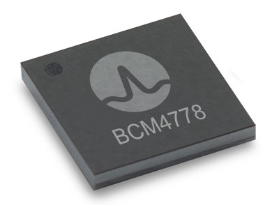
The BCM4778’s third-generation dual-frequency GNSS receiver features advanced multipath mitigation, L5 acquisition capability, LTE filtering and jamming protection
Broadcom Inc. has launched the BCM4778, its lowest power L1/L5 GNSS receiver chip optimized for mobile and wearable applications. Equipped with the latest GNSS innovations, the third-generation chip is 35% smaller and consumes five times less power than the previous generation.
Broadcom will be presenting further information on the chip in the Session B5, Panel: GNSS Chipset Technology – Trends, Opportunities and Challenges panel at the ION GNSS+ 2021 on Sept. 24.
Dual-frequency GNSS continues to be an important location feature for modern mobile and wearable devices, providing greater positioning accuracy for location-based applications. The advanced L5 signal enables sidewalk-level accuracy for pedestrian navigation in urban environments, as well as lane-level accuracy for vehicle navigation.
Reduction in GNSS power consumption is crucial to extending the battery life of a mobile or wearable device. Compared to GNSS receivers used in integrated platforms, Broadcom’s single-chip BCM4778 delivers significantly lower power consumption and higher performance while offering more advanced GNSS features, such as the next-generation Grid Tracking urban multipath mitigation technology.
“We are excited to see this impressive power reduction, combined with the L5 Grid Tracking technology in the new Broadcom GNSS chip. This will increase the impact of Google’s 3DMA ray-tracing for urban multipath mitigation,” said Frank van Diggelen, principal software engineer at Google.
Longer battery life. The BCM4778 increases the GNSS always-on battery life on a smartwatch by 30 hours compared to the previous generation chip operating on a 300-mAh battery. The extended battery life helps drive new experiences in smartwatches and phones, including keeping the GNSS always-on for fitness applications for multiple days on a single battery charge.
In addition, the BCM4778 features fully integrated LNAs for L1 and L5 bands, which reduces RF front-end BOM costs and footprint requirements, suitable for space-constrained applications. The chip offers increased flexibility to smartwatch and phone designers with its small size. Having the ability to place the BCM4778 closer to the antenna helps improve signal reception and enhances overall GNSS performance.
The BCM4778 dual-frequency chip is designed for small mobile and wearables. (Photo: Broadcom)
Product Highlights
7nm CMOS technology
Typical power consumption
4mW L1 band only
6mW L1+L5 simultaneous
FCBGA package
New Grid Tracking technology
Advanced multipath mitigation
Continuously tracks the full L5 channel
Capable of L5 acquisition
Increased processing capability and throughput
Advanced LTE filtering and jamming mitigation
Enhanced LTE Band 13 and Band 14 filtering
Spoofing and jamming detector
Jamming mitigation through multiband and multi constellation
Reduced BOM cost and footprint
Flexibility in using internal LNAs
Optional operation without interstage SAW filters
Integrated switching regulator with direct connect to battery
“With the launch of this third generation dual-frequency GNSS receiver chip, Broadcom continues the tradition of raising the bar for mobile GNSS,” said Vijay Nagarajan, vice president of marketing for the Wireless Communications and Connectivity Division at Broadcom. “Always-on dual frequency GNSS is a key request from mobile and wearable OEMs, and we are thrilled to deliver it.”
“Consumer electronic companies have been faced with the challenge of managing power consumption versus performance, often having to choose one over the other. Broadcom’s innovative approach to the BCM4778 allows their customers to realize improvements on both fronts,” said Ramon T. Llamas, research director for mobile devices at IDC. “The result: device manufacturers can enable new experiences and run applications over a sustained period of time. In addition, by reducing its BOM cost and its physical footprint, Broadcom is enabling further benefits from cost savings and design configurability.”
Broadcom is currently sampling the BCM4778 to its early access partners and customers. Please contact your local Broadcom sales representative for samples and pricing.
The webinar will be presented by Gerhard Kruizinga, navigation engineer, Mars 2020 Navigation Team chief, NASA’s Jet Propulsion Laboratory, and moderated by Frank van Diggelen, ION president.
“We are honored to have the Navigation team chief of this historic mission, Gerhard Kruizinga, present his first-hand account of getting NASA’s Mars 2020 Perseverance Rover from the launch pad to a safe landing on Mars,” van Diggelen said.
The precision landing required very high-precision interplanetary navigation and accommodation of entry guidance target requirements, planetary protection requirements and propellant allocation for trajectory correction maneuvers.
The main navigation objective was to predict the trajectory accuracy at atmospheric entry, such that the entry descent and landing system requirements were satisfied for a safe landing. This presentation discusses the planning to meet all navigation requirements and the actual navigation performance during cruise and landing.
Originally posted in the Android Developers Blog, the following is reprinted with permission from authors Frank van Diggelen, principal engineer, and Jennifer Wang, product manager, Google.
At Android, we want to make it as easy as possible for developers to create the most helpful apps for their users. That’s why we aim to provide the best location experience with our APIs like the Fused Location Provider API (FLP). However, we’ve heard from many of you that the biggest location issue is inaccuracy in dense urban areas, such as wrong-side-of-the-street and even wrong-city-block errors.
This is particularly critical for the most-used location apps, such as rideshare and navigation. For instance, when users request a rideshare vehicle in a city, apps cannot easily locate them because of the GPS errors.
The last great unsolved GPS problem
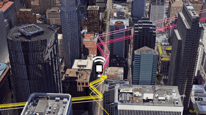
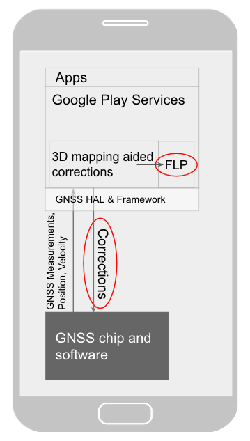
This wrong-side-of-the-street position error is caused by reflected GPS signals in cities, and we embarked on an ambitious project to help solve this great problem in GPS. Our solution uses 3D mapping aided corrections, and is only feasible to be done at scale by Google because it comprises 3D building models, raw GPS measurements, and machine learning.
The December Pixel Feature Drop adds 3D mapping aided GPS corrections to Pixel 5 and Pixel 4a (5G). With a system API that provides feedback to the Qualcomm Snapdragon 5G Mobile Platform that powers Pixel, the accuracy in cities (urban canyons) improves spectacularly.
Image: Frank van DiggelenImage: Frank van Diggelen
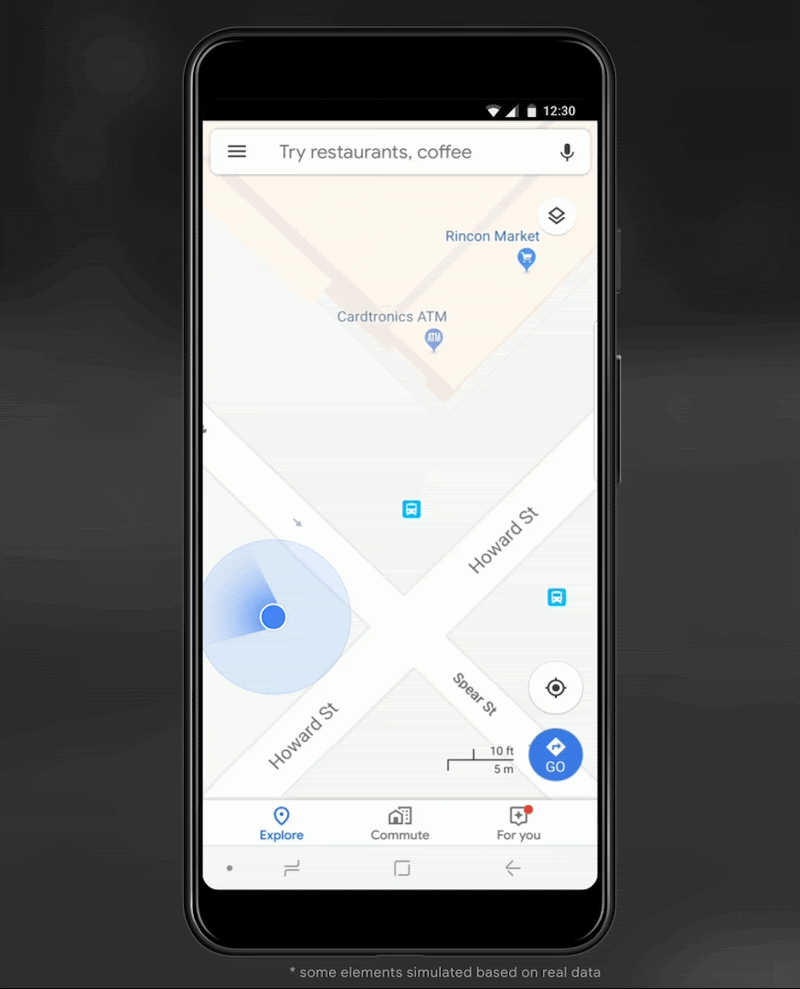
Pictures above show a pedestrian test, with Pixel 5 phone, walking along one side of the street, then the other. Yellow = Path followed, Red = without 3D mapping aided corrections, Blue = with 3D mapping aided corrections.
Why hasn’t this been solved before?
The problem is that GPS constructively locates you in the wrong place when you are in a city. This is because all GPS systems are based on line-of-sight operation from satellites. But in big cities, most or all signals reach you through non line-of-sight reflections, because the direct signals are blocked by the buildings.
Diagram of the 3D mapping aided corrections module in Google Play services, with corrections feeding into the FLP API. 3D mapping aided corrections are also fed into the GNSS chip and software, which in turn provides GNSS measurements, position, and velocity back to the module. (Image: Frank van Diggelen)Image: Frank van Diggelen
The GPS chip assumes that the signal is line-of-sight and therefore introduces error when it calculates the excess path length that the signals traveled. The most common side effect is that your position appears on the wrong side of the street, although your position can also appear on the wrong city block, especially in very large cities with many skyscrapers.
There have been attempts to address this problem for more than a decade. But no solution existed at scale, until 3D mapping aided corrections were launched on Android.
How 3D mapping aided corrections work
Image: Frank van Diggelen
The 3D mapping aided corrections module, in Google Play services, includes tiles of 3D building models that Google has for more than 3,850 cities around the world. Google Play services 3D mapping aided corrections currently supports pedestrian use-cases only. When you use your device’s GPS while walking, Android’s Activity Recognition API will recognize that you are a pedestrian, and if you are in one of the 3,850+ cities, tiles with 3D models will be downloaded and cached on the phone for that city. Cache size is approximately 20MB, which is about the same size as 6 photographs.
Inside the module, the 3D mapping aided corrections algorithms solve the chicken-and-egg problem, which is: if the GPS position is not in the right place, then how do you know which buildings are blocking or reflecting the signals? Having solved this problem, 3D mapping aided corrections provide a set of corrected positions to the FLP. A system API then provides this information to the GPS chip to help the chip improve the accuracy of the next GPS fix.
With this December Pixel feature drop, we are releasing version 2 of 3D mapping aided corrections on Pixel 5 and Pixel 4a (5G). This reduces wrong-side-of-street occurrences by approximately 75%. Other Android phones, using Android 8 or later, have version 1 implemented in the FLP, which reduces wrong-side-of-street occurrences by approximately 50%. Version 2 will be available to the entire Android ecosystem (Android 8 or later) in early 2021.
Android’s 3D mapping aided corrections work with signals from the USA’s GPS as well as other GNSS: GLONASS, Galileo, BeiDou, and QZSS.
Our GPS chip partners shared the importance of this work for their technologies.
Francesco Grilli, vice president of product management at Qualcomm Technologies Inc.:
“Consumers rely on the accuracy of the positioning and navigation capabilities of their mobile phones. Location technology is at the heart of ensuring you find your favorite restaurant and you get your rideshare service in a timely manner. Qualcomm Technologies is leading the charge to improve consumer experiences with its newest Qualcomm Location Suite technology featuring integration with Google’s 3D mapping aided corrections. This collaboration with Google is an important milestone toward sidewalk-level location accuracy.”
Charles Abraham, senior director of engineering, Broadcom Inc.:
“Broadcom has integrated Google’s 3D mapping aided corrections into the navigation engine of the BCM47765 dual-frequency GNSS chip. The combination of dual frequency L1 and L5 signals plus 3D mapping aided corrections provides unprecedented accuracy in urban canyons. L5 plus Google’s corrections are a game-changer for GNSS use in cities.”
Yenchi Lee, deputy general manager of MediaTek’s Wireless Communications Business Unit:
“Google’s 3D mapping aided corrections is a major advancement in personal location accuracy for smartphone users when walking in urban environments. MediaTek’s Dimensity 5G family enables 3D mapping aided corrections in addition to its highly accurate dual-band GNSS and industry-leading dead reckoning performance to give the most accurate global positioning ever for 5G smartphone users.”
How to access 3D mapping aided corrections
Android’s 3D mapping aided corrections automatically works when the GPS is being used by a pedestrian in any of the 3850+ cities, on any phone that runs Android 8 or later. The best way for developers to take advantage of the improvement is to use FLP to get location information. The further 3D mapping aided corrections in the GPS chip are available to Pixel 5 and Pixel 4a (5G) today, and will be rolled out to the rest of the Android ecosystem (Android 8 or later) in the next several weeks. We will also soon support more modes including driving.
Android’s 3D mapping aided corrections cover more than 3850 cities, including:
North America: All major cities in USA, Canada, Mexico.
Europe: All major cities. (100%, except Russia & Ukraine)
Asia: All major cities in Japan and Taiwan.
Rest of the world: All major cities in Brazil, Argentina, Australia, New Zealand, and South Africa.
As our Google Earth 3D models expand, so will 3D mapping aided corrections coverage.
Google Maps is also getting updates that will provide more street level detail for pedestrians in select cities, such as sidewalks, crosswalks, and pedestrian islands. In 2021, you can get these updates for your app using the Google Maps Platform. Along with the improved location accuracy from 3D mapping aided corrections, we hope we can help developers like you better support use cases for the world’s 2B pedestrians that use Android.
Continuously making location better
In addition to 3D mapping aided corrections, we continue to work hard to make location as accurate and useful as possible. Below are the latest improvements to the Fused Location Provider API (FLP):
Developers wanted an easier way to retrieve the current location. With the new getCurrentLocation() API, developers can get the current location in a single request, rather than having to subscribe to ongoing location changes. By allowing developers to request location only when needed (and automatically timing out and closing open location requests), this new API also improves battery life. Check out our latest Kotlin sample.
Android 11’s Data Access Auditing API provides more transparency into how your app and its dependencies access private data (like location) from users. With the new support for the API’s attribution tags in the FusedLocationProviderClient, developers can more easily audit their apps’ location subscriptions in addition to regular location requests. Check out this Kotlin sample to learn more.
Qualcomm and Snapdragon are trademarks or registered trademarks of Qualcomm Incorporated. Qualcomm Snapdragon and Qualcomm Location Suite are products of Qualcomm Technologies Inc. and/or its subsidiaries.
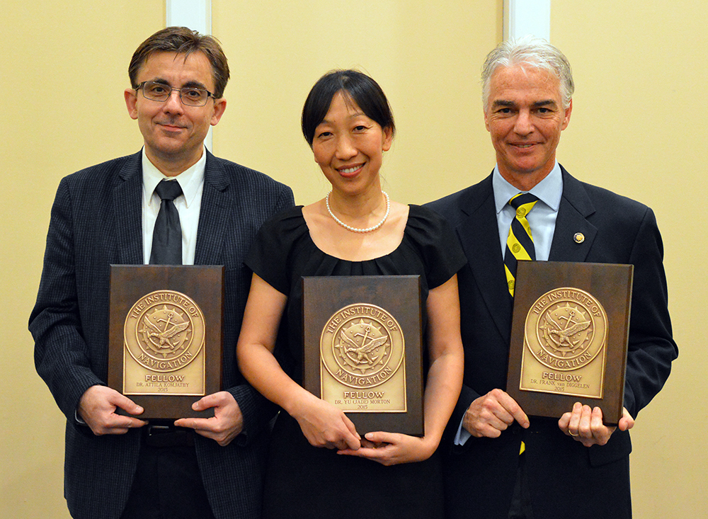
The Institute of Navigation (ION) presented its Annual Awards during the ION International Technical Meeting in Dana Point, Calif., Jan. 26-28. The annual awards recognize individuals making significant contributions or demonstrating outstanding performance relating to the art and science of navigation. ION also announced its elected Fellow members.
Award Winners
Mathieu Joerger received the Early Achievement Award for outstanding contributions to the integrity of multi-constellation and multi-sensor navigation systems. The award is presented in recognition of outstanding contributions made early in one’s career.
Captain Samantha Ekwall received the Superior Achievement Award for her heroic actions as the lead navigator for a five-ship formation during the refueling of the battle damaged CV-22 Ospreys during a U.S. embassy evacuation attempt in South Sudan. The Superior Achievement Award is presented to an individual demonstrating outstanding accomplishments as a practicing navigator.
Hamid Mokhtarzadeh and Demoz Gebre-Egziabher received the Dr. Samuel M. Burka Award for their paper “Cooperative Inertial Navigation” published in the Summer 2014 issue of NAVIGATION: Journal of the Institute of Navigation, Vol. 61, No. 2,pp.77-94. The award recognizes outstanding achievement in the preparation of a paper contributing to the advancement of the art and science of positioning, navigation and timing.
Patricia Doherty received the Captain P. V. H. Weems Award for her contributions to the management and encouragement of advanced navigation research and for her service to ION. The award is presented to individuals for continuing contributions to the art and science of navigation.
Bruce Haines received the Tycho Brahe Award for notable achievements in astrodynamics-navigation, precise orbit determination and satellite applications to geophysics and oceanography. The Tycho Brahe Award is presented to recognize outstanding contributions to the science of space navigation, guidance and control.
Neeraj Pujara received the Norman P. Hays Award for his inspired leadership, outstanding encouragement, inspiration and dedicated support contributing to the advancement of navigation. The award is given in recognition of outstanding encouragement, inspiration and support contributing to the advancement of navigation.
Todd Humphreys received the Thomas L. Thurlow Award for contributions that enhance radionavigation security and robustness in the face of intentional spoofing and natural interference. The award recognizes outstanding contributions to the science of navigation. Humphreys has written several articles for GPS World, the latest being the February cover story, “Accuracy in the Palm of Your Hand.”
Patricia Doherty received the Distinguished Service Award, presented for extraordinary service to ION.
ION’s new Fellows: (from left) Attila Komjathy, Yu (Jade) Morton, and Frank van Digglen.
Fellows
ION also announced recipients of 2015 Fellow memberships. Election to Fellow membership recognizes the distinguished contributions of ION members to the advancement of the technology, management, practice and teaching the arts and science of navigation; and/or lifetime contributions to ION.
Attila Komjathy has been elected for contributions to remote sensing of Earth’s ionosphere using GNSS signals.
Yu (Jade) Morton has been elected for contributions to GNSS software receivers and the development of a worldwide network of space weather monitoring stations.
Frank van Digglen has been elected for contributions to satellite-based navigation for consumer applications, especially mobile handheld devices. van Diggelen joined the GPS World Advisory Board in 2014.
In the June issue’s cover story, “Interchangeability Accomplished,” is a paragraph headed, “Satellite Intersystem Biases,” which appears to assert that Galileo System Time (GST) is 3 seconds ahead of UTC.
However, in the version of the Galileo Signal In Space Interface Control Document posted at: http://ec.europa.eu/enterprise/policies/satnav/galileo/files/galileo-os-sis-icd-issue1-revision1_en.pdf, paragraph 5.1.2 appears to indicate that Galileo System Time (GST) was synchronized, at the second level, with GPS time on 22 August 1999 (that is, 13 seconds ahead of UTC). And, given that a) GST, like GPS time, does not step for announced leap seconds, and b) the IERS has, as of today, announced 3 leap seconds since 22 August 1999, such would appear to suggest that GST is presently roughly 16 seconds (vice 3 seconds) ahead of UTC.
— Stuart Eventhal Fountain, Colorado
Author Frank van Diggelen replies:
Yes! You are right, the article should have said 16 seconds for Galileo, not 3. Thanks for catching that. I’ve corrected the text that appears in the online version of the article, and the accompanying figure.
Media Scoop
The online article covering Javad Ashjaee’s input on the GLONASS situation makes a positive statement that clarifies what has been a horrible reporting job across the board by news channels.
Fox, CBS, NBC, and ABC should all be ashamed that GPS World scooped them on what appears to be a simple story.
Good work.
— Mark Silver IGage Mapping Corporation Salt Lake City, Utah
To Consumer-Grade GNSS Chip Manufacturers
I would like you to consider including a very simple feature in your GPS functionality that will permit elevation to be identified to decimeter level in many instances. The changes needed to the chip are simply the ability to accept an accurate latitude and longitude input, and an elevation calculation function that uses input latitude and longitude.
In addition to enabling instantaneous calculation of an accurate elevation, it may be that a “residual better accuracy” will remain for some time after the calculation, and that this will permit substantially improved latitude and longitude identification at a close distance.
The geo-location scene has evolved rapidly over the past 20 years. It is now very commonplace to be able to locate the latitude and longitude of a location extremely quickly and extremely accurately. For instance, the Google Earth image from the front of my house shows the dotted dividing line in the center of the road. Measuring one of these lines in Google Earth gives a size of 3.1 meters by 20 to 30 cm wide. The lines actually measure 3.0 meters by 12 cm wide. From within Google Earth I can identify the latitude and longitude of the end point on the centre of this line to within ±10 cm with a high degree of confidence. In addition there may be some other small errors in Google’s reporting of the latitude & longitude (for example due to placement of the image or distortion of the image), but these are hopefully minimal.
Now if I place my GPS unit on the end center of this line in the road, I am provided with a result that I know is erroneous. The GPS horizontal location shown in Google Earth is very rarely within two meters of my known location. It is known that altitudinal accuracy is always some two times worse than horizontal accuracy.
If I can simply tell the GPS unit that I am at this known horizontal location, it is a relatively simple calculation to recalibrate the clock and pseudoranges to provide my elevation, which will have an accuracy of a two times the accuracy of the horizontal position. Decimeter horizontal accuracy will provide 2-decimeter altitude accuracy. This is close to 100 times better than the elevation accuracy currently available on any consumer grade stand-alone device and is also effectively instantaneous!
This functionality is simple to implement. I would hope that it could be implemented with nothing more than an upgraded ROM which includes a new API function to allow the input of “I know this is my current horizontal location” and an enhanced calculation process which uses this horizontal location to calculate altitude.
I am unsure whether a residual improvement in accuracy can be attained. Even an improved accuracy for 1 minute after the fix would be useful in many situations, and an improved accuracy for 5 to 10 minutes would be a boon.
GPS World contributing editor Eric Gakstatter gave a talk on predicted ephemeris at the Civil GPS Service Interface Committee (CGSIC) on Tuesday. The talk was invited and the topic was suggested by CGSIC coordinators. The 53rd meeting of the CGSIC was held Monday and Tuesday before the Institute of Navigation GNSS+ 2013 Conference. Here is Eric’s talk:
Whenever I point a critical finger at the GPS folks, I apologize before I do so because it’s really a wonderful system.
What I try to offer the community in general is a link between the GPS system operators and the civil community. It’s amazing when you think about it, two huge user bases of civil and military users, and a little strip called CGSIC that communicates between them. Rick [Hamilton of CGSIC] introduced me to this concept a couple months ago and asked me to investigate it and think about it. This is what I researched and talked to some folks and came up with.
First, I want to introduce you to some folks doing fascinating things with GPS.
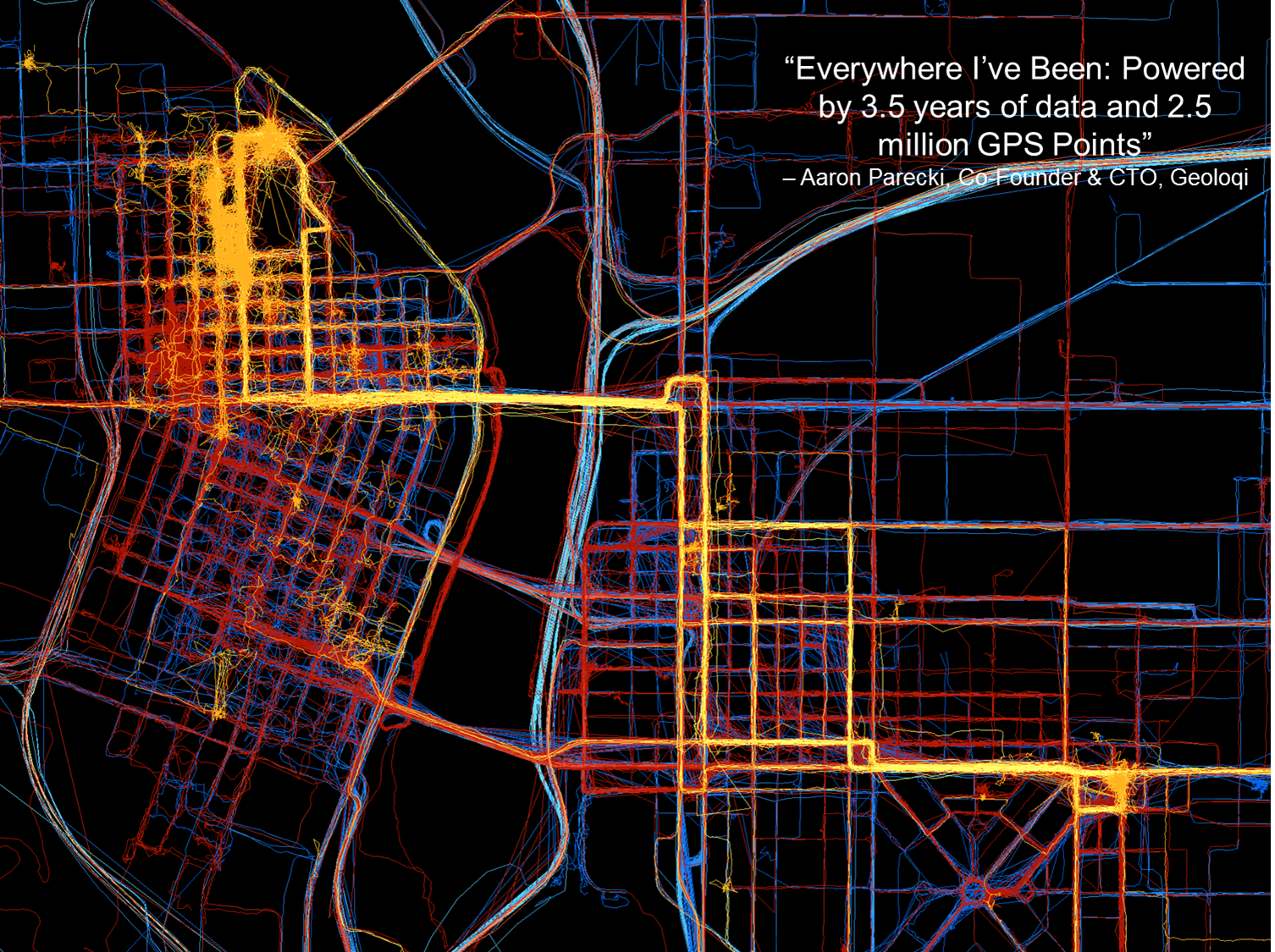
Here’s a young company, Geoloqi, doing really interesting things in Portland. They don’t have any clue where GPS came from; they just have it on their smartphones. One of the founders collected GPS data everywhere he went for the last three and a half years. This map shows 2.5 million data points, and I think it’s fascinating.
This map of Portland by Geoloqi has 2.5 million data points.
These folks interface between the GPS chipset in the mobile device and the apps that run on it. They sold their company to Esri last year.
“Geolocation has the potential to become an indispensable part of our lives. But to be a valuable service, the technology needs to be invisible yet opted into, private, and secure.” — Amber Case, Geoloqi founder
These kids just want to get things done, create ideas and create products: things like, check into a hotel when you get within 100 yards of the door; get your prescription prepared and ready for you when you come within a certain distance of a pharmacy. All these kinds of things are based on the geotrigger or geofence concept.
Now, talking about my work, primarily in surveying and mapping, with companies like utilities with 15 million customers and a lot of infrastructure. To put that at the fingertips of a maintenance person, that’s pretty amazing. I’ve been swimming in this soup for a long time, and I hadn’t heard of this concept — the predicted ephemeris (PRED) produced by GPSOC.
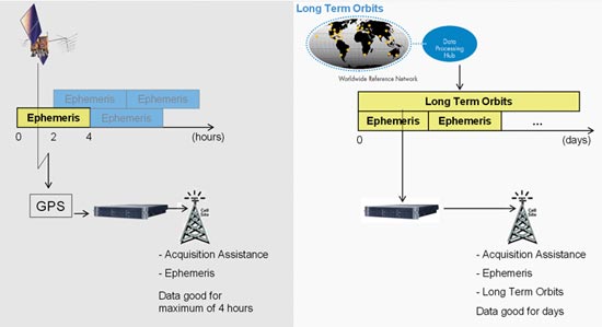
Take a PRED state vector data file, which is currently generated every 15 minutes by the GPS Operations Center under For Official Use Only (FOUO), currently designated unclassified, but not accessible to the general public. If it were made available for public use, it could decrease time to first fix from 40 seconds when you turn on your mobile device, to 5 to 10 seconds.
In the high-precision field like mine, surveying, it really doesn’t make too much difference because by the time you get out of your truck and set up your gear, 30 seconds has already gone by and it doesn’t make much difference.
Now it could be more of an issue with mobile devices in GPS-impaired environments such as urban canyons or indoor environments, where 30 seconds could make the difference between getting a fix or not.
If predicted ephemeris were available, developers could distribute it terrestrially via a wireless network to mobile devices.
Problem: How to transfer PRED from a U.S. government FOUO environment to make it available to application developers?
To me as a product developer or a product manager, interested in pushing products out to the community, that’s a really small speed bump. But when I talk to colleagues who operate in that (government) space, that’s a significant undertaking, a real obstacle. We’re talking about a big change, and a big process to go through to effect that change.
PRED from the horse’s mouth, so to speak, from the U.S. Air Force, really builds credibility. I can build it into a product, because I know it’s going to be there three or four or more years from now.
PRED can be made available, but Civil GPS app developers need to speak up — because civil users won’t. They don’t know about it. They don’t know what is possible.
“How does somebody know what they want if they haven’t even seen it?” — Steve Jobs
I’m trying to raise awareness here. I’ll probably write about soon in the magazine or in my [Survey Scene] email newsletter.
Frank van Diggelen, Broadcom. We’ve been doing this in the commercial world for over a decade. You all have it in your cellphones, with about 90% likelihood provided by Broadcom or someone who’s licensed our patents. It doesn’t work properly unless you have the source of the data and the client side working very cooperatively. The issue is the . . . gap between prediction and use. If the satellite is moved (in orbit or clock) then the prediction is wrong, and you need client-side software that is design cooperatively with the predictions. Our predictions are available in 2-, 4-, 7- or 30- day intervals. Think of a use case where you get a seven-day prediction, and then go away from network coverage for several days, meanwhile, say on Day 4, a satellite is moved or has its clock adjusted, on Day 5 it is set healthy, on Day 6 you turn on your handset and use the prediction from six days ago — it will be wrong and your client-side software has to catch that and know know how to invalidate the predictions.
We deliver these orbital predictions at about the rate of a billion per month. It’s been there for 10 years, and its been working so well most people aren’t even aware that it’s there. If the Air Force puts these out, that sounds great, but if you don’t have client-side software looking for erroneous predicitions — when a satellite is adjusted or moved — then things would be a lot worse for the user community than they have for the last 10 years.
Eric Gakstatter: I understand that, but that’s true for any technology. If a company implements it incorrectly, the market will reject it. Let the market decide.
There may be a need for a non-proprietary solution (PRED) that is publicly available so it could be implemented by other developers, and level the playing field to increase market adoption of GPS.
A new method enables the mobile phone to compute its own position using acquisition assistance data with increased resolution in some of the fields. It benefits network operators as they can deliver the best performance with minimum bandwidth requirements, making this especially relevant in emergency-call situations.
By Javier de Salas and Frank van Diggelen
In assisted GPS (A-GPS) and A-GNSS, some information in the form of assistance data is sent to the mobile terminal equipped with a GNSS receiver. This data helps the receiver acquire satellite signals faster and at lower power levels as well as compute its own position. Assistance data is essential in many GNSS use cases but it is especially relevant in emergency calls from mobile terminals (e911, e112) where a fast response and the best sensitivity are required. Mobile subscribers are often in environments where direct satellite visibility is impaired because the user is inside a building or there are other obstructions. Emergency situations also require a very fast response (time-to -first-fix or TTFF), typically within 30 seconds, so the performance requirements imposed on the GNSS receiver are very stringent.
GNSS assistance data is standardized by 3GPP and 3GPP2 in two different types, broadly known as mobile-station (MS) based and MS-assisted. MS-assisted positions are computed by a server. MS-based methods enjoy certain performance benefits in position accuracy and response time when compared with MS-assisted methods. However, the amount of assistance data required for MS-based operation is substantially larger than the assistance data required by MS-assisted methods.
For this reason, some network operators choose the MS-assisted methods for their emergency-call services. Larger bandwidth requirements are of deep concern if many callers demand the services at the same time, because network capacity could be challenged when it is most needed.
This article describes a method that enables the mobile terminal to compute its own position, thus enjoying the benefits outlined above but with the same assistance data as in MS-assisted methods, only with increased resolution in some of the fields. We call this method single-shot MS-based. Network operators benefit because they can deliver the best performance with the minimum bandwidth requirements, especially relevant in emergency call situations.
Some 3GPP specifications will need to be modified slightly to increase the resolution of the relevant assistance data fields, namely, 3GPP TS 44.031, 3GPP TS 25.331, and 3GPP TS 36.355
Bandwidth versus Performance
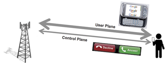
Assisted GNSS information is exchanged between the location server and the mobile device using standardized protocols. Several bodies create different specifications: 3GPP, 3GPP2, and the Open Mobile Alliance (OMA). Broadly speaking, we can say that 3GPP and 3GPP2 work on protocols that are used over control plane and OMA works on protocols that are used over user plane.
Control plane refers to the use of cellular signaling channels as the transport mechanism for the assistance data and position information. User plane refers to the use of traffic channels (see Figure 1). When you get a phone call, the control plane makes your phone ring. When you browse the web you are using the user plane.
Figure 1. Control plane is used for signaling purposes, user plane for transferring user data.
Signaling channels are not designed to transfer large amount of information, so it is important for 3GPP and 3GPP2 to make the protocols efficient and save bandwidth while maintaining the best performance. Cellular traffic channels are designed to transport much larger amounts of data and thus the bandwidth restrictions are less important than in the control plane case; OMA typically addresses richer GNSS features for Location Based Services (LBS). This is why network operators often support emergency call location using control plane, leaving the user plane for commercial applications. It is also a very good way to separate emergency traffic from LBS traffic so that the former is never compromised by lack of capacity coming from heavy use of commercial location applications.
Two different types of assisted GNSS have been standardized, known as MS-based and MS-assisted in Global System for Mobile Communicatios (GSM) and code-division multiple-access (CDMA) specifications, and as user-equipment (UE) based and UE-assisted in Wideband Code Division Multiple Access (WCDMA) specifications.
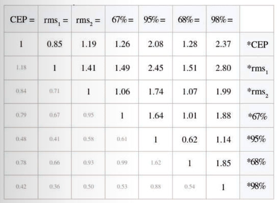
MS-assisted refers to the case where the mobile device equipped with a GNSS receiver does not compute its own position but it is instead computed in a location server in the operator’s network. Assistance data is sent to the mobile device to help acquire satellite signals faster. Remember that GNSS signal acquisition involves a three dimensional search (satellite, frequency and delay) that requires intensive signal processing. So assistance data is sent in the form of visible satellites including expected delays and expected Doppler shifts. These values are provided at a reference time and relative to an approximate location for the subscriber. The approximate location typically comes from the location of the serving cell tower. The reference time, but not the approximate location, is normally included as part of the assistance data. After a certain number of satellites are acquired, measurements are sent back to the location server for it to compute the subscriber position. GNSS measurements for each satellite include the measured delay, measured Doppler frequency and an estimation of the signal power to noise ratio. Assistance data in MS-assisted is referred to as “acquisition assistance”. It contains the minimum information so it is very efficient in bandwidth. See Table 1 for an exact bit count of the GNSS acquisition assistance. This table will be used as an example throughout this paper. In this particular example, it is assumed that assistance data is sent for 16 satellites.
MS-based refers to the case where the GNSS-enabled mobile device computes its own position locally. A different set of assistance data parameters are sent to the device to help it acquire the GNSS signals as well as calculate its own geographical location. Measurements are processed by the mobile device internal circuitry until the locally computed position is deemed accurate enough to meet the requirements received in the location request or a timeout is reached. Location information (latitude, longitude, altitude) is then sent back to the network in response to the location request. Assistance data in MS-based consists, at a minimum, of three elements: an approximate location (coming from the serving cell), an approximate time (accurate to a few seconds) and a description of the satellite orbits and clock errors referred to in the specifications as navigation model. See Table 2 for an exact bit count of the GPS assistance data in MS-based. The GNSS receiver uses the approximate location, the approximate time and the navigation model to estimate the expected delays and Doppler shifts of the visible satellite and thus proceed to the acquisition of satellite signals very much like in the MS-assisted case. Satellite measurements (code delays in the simplest implementation) and navigation model are used to calculate the receiver’s own position as explained below.
Advantages of MS-Based over MS-Assisted
We can see from Tables 1 and 2 that the amount of data used in MS-based i
s significantly larger than that of MS-assisted, in fact by a factor of seven! So why do some operators still decide to use MS-based over MS-assisted? The answer is there are noticeable performance advantages when using MS-based. An in-depth description of these advantages is out of the scope of this paper; but we will provide descriptions of what we see as the three more important ones.
Better Estimate of Position Accuracy. The first advantage lies with the fact that in MS-based mode the mobile device has a much better knowledge of the estimated accuracy of the position that it has computed internally. This was implicitly mentioned in the description of the MS-based and MS-assisted method above when we explained that in MS-assisted mode, the mobile terminal sends the measurements after a sufficient number of satellites (with certain range uncertainties) have been acquired. This is precisely the problem, what is a sufficient number of satellites? It is not easy to know for the mobile receiver because it does not know what positioning algorithm or what satellite subset the location server will use in its calculations. As such, it is more difficult to guarantee the quality of service of the position in the MS-assisted method. One could perhaps argue that the mobile receiver has an idea of the satellite geometry based on the Azimuth and Elevation fields (see Table 1) and therefore can perform a more educated estimation than just using the number of satellites and their associated uncertainties. This argument will only be valid if the mobile device knew exactly what the satellite subset is that the location server will employ in its position computation. Different satellite subsets yield different estimated accuracies. In addition to this, azimuth and elevation fields are optional in other positioning protocols such as Radio Resource Location Protocol (RRLP) and Radio Resource Control (RRC) and are also quantized with a value of 11.25 degrees, which deems them practically useless to quantify the satellite geometry in the critical cases where the dilution of precision (DOP) values are large.
Kalman Filter. The second advantage comes from the use of sophisticated navigation filters (for example, Kalman filters) by all GNSS manufacturers. In the MS-based method, the final position estimate that is sent to the network is computed using consecutive sets of measurements that help the position converge using the receiver dynamic model to smooth the resulting positions for greater accuracy. Conversely, in MS-assisted mode, the position computation engine only has access to a single set of measurements and therefore cannot employ sequential navigation filters.
Coarse-Time A-GNSS. The third advantage is perhaps the more difficult to grasp. It has to do with the fact that most (if not all) A-GNSS location servers only provide reference time information that is accurate to within a few seconds. On the other hand, for classical GNSS position computation, knowledge of absolute time accurate to a few milliseconds is required. Typically, it is the task of the GNSS receiver to decode the accurate satellite time information that comes modulated on the GNSS signals as part of the navigation message. However, in environments where satellite visibility is impaired, such as indoors, the satellite signals may be so low that the timing information cannot be decoded from the satellite due to excessive Bit Error Rate. In these situations, the absolute time can be set as an additional state that to be solved as part of the complete navigation solution therefore increasing the position yield in of the GNSS receiver in difficult environments. We refer to this technique as coarse time A-GNSS.
There is no technical reason why this technique could not be implemented in a location server in the operator’s network as opposed to the mobile device itself. However, for this technique to work properly, the mobile device should indicate to the location server whether or not it has successfully decoded the time from the satellites signals (or perhaps other sources). This is normally done by setting an associated time-uncertainty value with the time reported with the GPS measurements. There are some 3GPP specifications (for example RRC prior to R7) that do not support this parameter so they have hindered the adoption of the coarse time A-GNSS technique in MS-assisted mode.
Continuous Navigation. By delivering ephemeris data (good for several hours), MS-based techniques have an advantage over MS-assisted for continuous navigation. This advantage is not addressed further in this article, where we are focused only on first fixes.
Single-Shot MS-Based Method
We present a brief reminder of how GNSS positions are computed in order to determine what assistance data is strictly needed for a mobile terminal to compute its own location. We will use a simple least squares algorithm for simplicity but the conclusions are extensible to the cases of other positioning algorithms such as Kalman filters.
The observation equations are typically linearized around an approximate location. They can be easily presented in matrix form as:
Δ y = A Δ x
where Δ y is a column vector [m x 1] containing the difference between the predicted and measured pseudo-ranges for the m satellites measured by the GNSS receiver. The predicted pseudo-ranges can be obtained using the acquisition assistance data (codePhase and intCodePhase fields.)
Δ x is a column vector [4 x 1] containing the change in the “state” from the approximate position. The state has four unknowns x, y, z and b. x, y, and z are the change in the local East (longitude axis), North (latitude axis) and Up (altitude axis) coordinates from the reference position, b is the common mode error (mostly from the internal receiver clock error) in distance units.
A is an [m x 4] matrix, the first three elements in each row ux , uy , uz are the coordinates of the unit vectors from the receiver to the satellite, the last element is a 1 for the common mode error. A is sometimes referred as the geometry matrix.
Coordinates of unit vectors can be written as a function of the azimuth and elevation of each satellite. Simple trigonometry yields:
ux = cos (el) * sin (az)
uy = cos (el) * cos(az)
uz = sin(el)
In the coarse-time case there will be a fifth column of A containing the range rates, which are provided in the MS assistance data.
The goal is, of course, to determine the change in the state (our unknowns). Using simple least squares
Δ x = (ATA)–1AT Δ y
we can easily determine Δx. The coordinate changes in Δx (delta position) will be applied to the approximate location to obtain the new position.
Assistance Data Required
To re-cap from the previous section, we have seen that to compute Δx we need:
Expected pseudo-ranges for satellites in view (from acquisition assistance)
Measured pseudo-ranges (from the GNSS receiver)
Azimuths and Elevations for the geometry matrix (from acquisition assistance)
It would seem that if the mobile device receives acquisition assistance and measures the pseudo-ranges for a few satellites, it has everything that is required to compute a position (or at least a delta position) inside the GNSS mobile device. The delta position is relative to the position used to compu
te the acquisition assistance. Have we achieved our goal of computing position inside the mobile device with acquisition assistance? Not quite. Let’s now look at the acquisition assistance data in more detail.
We explained that we obtain the required expected pseudo-ranges from the acquisition assistance fields codePhase and intCodePhase. The codePhase field is defined with a resolution of one GPS chip, equivalent to 300 meters. Recall that we subtract the expected pseudo-range from the measured pseudo-range before we use the measurements in the position solution so this means if our expected pseudo-range was in error by, say, 150 meters because of the low resolution of this field, this is similar to making a measurement error of that amount, which of course will cause an unacceptable position error. This means the resolution of the codePhase field would need to be increased to be able to compute position. For a resolution of 2 meters, 8 more bits would need to be added.
The second topic of interest relates to the azimuth and elevation fields. These are needed to construct the geometry matrix A. As mentioned before, in 3GPP location protocols the azimuth and elevation of the acquisition assistance element are defined with a resolution of 11.25 degrees. Sines and cosines (needed to calculate the coordinates of the unit vectors) with such large angle errors will also yield large position errors. In Long-term Evolution Positioning Protocol (LPP), the situation has improved with the resolution being 0.7 degrees.
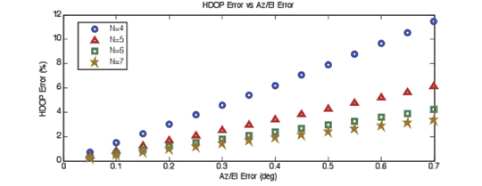
In an effort to quantify how the angle quantization affects the position error, we have run simulations that plot the 95 percentile of the HDOP error as a function of the angle error in azimuth and elevation (see Figure 2.) HDOP is proportional to the position error so this seems to be a reasonable choice. N is the number of satellites used in the simulations. As you might expect: the fewer the satellites the greater the effect.
Figure 2. HDOP error vs Az/El error. We use HDOP as a proxy for the expected position error: if the HDOP changes by 10 percent, we expect the position error to change by a similar amount.
We can see from the plot in Figure 2 that for an angle resolution of 0.7 degrees as currently defined in LPP, the 95 percent HDOP error is under 12 percent. If we wanted to make the worst error (N=4) under 2 percent, we can see that the resolution should be increased to 0.1 degrees. In order to meet this goal, 3 more bits would need to be added to both the azimuth and elevation fields in the acquisition assistance.
Another effect that must be noted is the possible change in the azimuth and elevation from the time the assistance data is received to the time the receiver computes its position (or delta position). In an emergency call scenario, typically we assume this time will not be greater than 24 seconds. Note the total allowed response time for an E-911 call is 30 seconds, including call establishment and network latencies. Simulations based on satellite geometry show that the worst-case effect is approximately of the same order of magnitude as the angle resolution discussed above, and therefore its impact in HDOP is just a few percentage points in the case of N=4.
At this point we seem to have everything we need to compute positions (or delta positions) inside the mobile terminal with the same acquisition assistance used in MS-assisted; albeit with slightly higher resolution in some of the fields.
To facilitate the comparison with MS-assisted and MS-based methods, Table 3 summarizes the exact bit count needed for Single Shot MS-based.
Optionally, if an absolute position is required in the mobile device instead of delta position, it would also require the approximate position (reference location) to be sent along with the rest of the assistance data (acquisition assistance, reference time). However, the MS-based performance advantages listed above can all be realized without the reference location, using only delta position. This is why we have not included Reference Location as an element that is needed for Single Shot MS-based.
Conclusions
We have seen that Single Shot MS-based can be used to enable all the MS-based performance advantages with, essentially, the same assistance data that is used in MS-assisted. Minimal additional bandwidth is required due to the increased resolution of some of the fields. Single Shot MS-based is therefore the best option for network operators that deploy A-GNSS based emergency location.
Not only does MS-based require significantly more bandwidth than MS-assisted (~ 7x) or Single Shot MS-based (~ 6x); but the absolute difference will increase with additional GNSS satellites such as GLONASS, SBAS, QZSS, Compass, and Galileo. Imagine all navigation models have to be sent for all satellites in view and for all GNSS constellations! Acquisition assistance can easily be made generic for every GNSS constellation since it is just “range and Doppler” and, in fact, this is the way it has been conceived in LPP where the dynamic ranges for all parameters are no longer restricted to GPS but allow other GNSS constellations.
Javier de Salas is director of GPS product marketing at Broadcom. Previously he worked at Ashtech, Magellan, and Global Locate. He has an MS in electrical engineering from Universidad Politecnica de Madrid.
Frank van Diggelen is chief navigation officer and senior technical director for GNSS at Broadcom. He is also a consulting assistant professor at Stanford University and is the author of A-GPS: Assisted GPS, GNSS and SBAS. He holds more than fifty issued U.S. patents on A-GPS and has a Ph.D. in electrical engineering from Cambridge University.
More Satellites, More Sensors Take Urban Navigation Downtown and Deep Indoors
By Frank van Diggelen
As we all know, GPS is practically perfect in every way — as long as it’s outside and unobstructed. Even cell phones can now produce meter-level accuracy under open sky. There are still many deficiencies in state-of-the-art location, particularly in deep urban canyons and inside large buildings. Which technologies will lead personal navigation into the future?
As we all know, GPS is practically perfect in every way . . . so long as it’s outside and unobstructed. Even cell phones can now produce meter-level accuracy under open sky. And, with Assisted GPS (A-GPS), those cell phones have mitigated the two great deficiencies of the original GPS: slow time to first fix (TTFF), and outdoor-only operation. A-GPS receivers can produce TTFF as fast as one second after a cold start, and (sometimes) work indoors.
However, there are still many deficiencies in the state of the art of location, particularly in deep urban can yons and inside large buildings. In the latter you will soon notice that even if your A-GPS operates in your house, it does not operate everywhere. The term “indoor GPS” is rather like “off-road vehicle”: your four-wheel drive may let you cruise down the beach, but you certainly cannot use it to climb every mountain nor ford every stream. Similarly “indoor GPS” denotes the presence of a capability — not the absence of all limitations.
And so what is the future of urban and indoor navigation, and which technologies will prevail? The short answer is: more satellites and more sensors. In this article we’ll look at the technologies that will move us from the era of GPS-only into the future of GPS-plus.
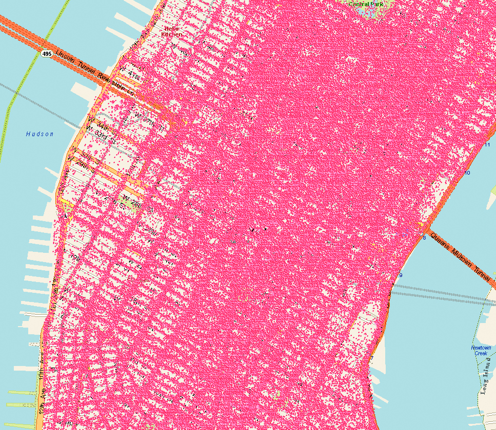
This is Manhattan.This is Manhattan on Wi-Fi.
Other GNSS
The most likely addition to GPS will be the other global navigation satellite systems, and all GPS receivers will be replaced by true, multi-system, GNSS over the next two to three years. Not because this will ever fully solve indoor location, but because of the outdoor problem in deep urban canyons.
When asked why he wanted to climb Everest, George Mallory famously said “because it is there.” Of the various GNSS systems, those with the most influence in the next few years will be GLONASS, because it is there, and QZSS because (as Mallory might have added) it is high. The first QZSS satellite recently began functional transmission. So let’s use QZSS as an example of why extra satellites are so important in the deep urban canyon.
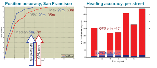
Figure 1 shows Shinjuku, Japan, a typical deep urban canyon and a terrible place for GPS. The blue dots show the positions of a GPS receiver. The white and orange lines show the actual line-of-sight vectors to the GPS satellites. The white lines are to GPS satellites in direct view. The orange lines are to satellites behind buildings. However, the high-sensitivity A-GPS receiver tracks all these satellites, by acquiring and tracking reflected signals. Thus the whole concept of GPS — of measuring distance by time-of-flight — breaks down. The reflected measurements are inaccurate because of the extra path length. And even if the receiver could somehow tell orange lines from white, the horizontal dilution of precision (HDOP) of the white-only lines is 58 in this real-life example. Now add two high-elevation satellites, shown by green lines, and things are much better. The green lines show the location of two QZSS satellites, and the HDOP of the five green + white satellites is 3.
Figure 1 shows the problem of the deep urban canyon, and the value of extra satellites. The problem is that there are not enough satellites in direct view. This puts receiver designers in an insoluble dilemma: Track only strong satellites, and you will not have enough; or track weak satellites, and you will measure reflections with large measurement errors because of the extra path length of the reflection. Moreover, the reflected signals can be indistinguishable from direct signals in their characteristics, especially in mobile phones where the antennas are poor, and directional — so that signal strength is not a reliable indicator of whether a signal is direct or not.
This example should put to rest the false notion that extra high satellites will not improve HDOP. In this case the HDOP improves by about 20 times, from 58 to 3. It is easy to find many similar examples using GPS + GLONASS or any other GNSS combination. More often than not, extra satellites improve the situation significantly.
The QZSS system uses inclined geostationary orbits to provide high elevation coverage above Japan (and, as a by-product, neighboring regions.) In this respect it is unique amongst the major GNSS: it is exclusively designed to provide good urban coverage of its home region. Compass has a similar component, but ultimately it, like GPS, GLONASS, and Galileo, has global ambitions.
Some other satellite systems, such as satellite radio, use inclined geostationary orbits like QZSS. With QZSS providing an alternative example of a new GNSS, European taxpayers might well ask why Galileo should provide medium-Earth orbit satellites that spend more time over America and Asia than over Europe. As a U.S. taxpayer, I’m all in favor of the current Galileo plan — after all, the United States has been sending GPS satellites over Europe for the last 30 years, so a little reciprocation seems only fair.
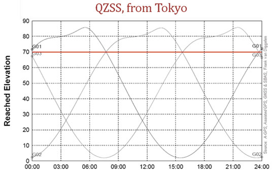
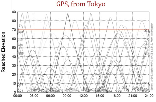
Figures 2 and 3 show how the three satellites of QZSS provide better high-elevation coverage over Tokyo (and neighboring regions), than all of the 30 GPS satellites combined.
QZSS-capable chips are already found in mobile phones and tablets available in the Asian market. As this article was being written, a Broadcom BCM4751 chip in Tokyo was computing the first-ever GPS+QZSS position.
Figure 2. Elevation above horizon of the QZSS satellites, as seen from Tokyo. Note that the inclined-geostationary orbits of the QZSS system have been designed so that there is always one satellite above 70°.Figure 3. Elevation of GPS satellites as seen from Tokyo. About half the time none of the 30 GPS satellites is above 70° elevation, a quarter of the time one GPS satellite is above 70°, a quarter of the time two GPS satellites are, and for half an hour three GPS satellite are. The three satellites of the QZSS constellation provide better high-elevation coverage in Tokyo than the 30 GPS satellites.
Wi-Fi
After GNSS, the second-leading location technology is wireless local area networks, commonly known as Wi-Fi. Wi-Fi location works by using a database of media access control (MAC) addresses and locations. When a mobile device senses a Wi-Fi access point, the MAC address and database give the location of the access point (AP). A simple average of many APs gives position accurate to tens of meters.
Wi-Fi location is already tightly integrated with GPS in many smartphones. Wi-Fi location accuracy is good enough that it is often mistaken for GPS, especially in cities where the density of APs is large. In Manhattan, for example, there are more than 25,000 APs per square kilometer (see opening figure.)
Several major companies, including Apple, Broadcom, and Google, have worldwide databases of Wi-Fi AP
locations that are used in mobile devices, especially smartphones and tablets.
MEMS, Accelerometers, and Gyros
The micro-electromechanical systems (MEMS) technique etches the silicon on a chip to exploit its mechanical and electrical properties. A MEMS chip, such as a chip-level accelerometer or rate gyro, thus has tiny moving parts that can sense acceleration or rate of turn, respectively. Both sensors are already common in smartphones, where they are used to set the correct screen orientation (portrait or landscape), and for gaming. Because they are already there, they are a natural addition to location technologies, and many companies are moving rapidly to integrate motion sensors with GPS for improved accuracy indoors and in urban canyons.
As an example of the benefits of MEMS motion sensors, Figure 4 shows a test case where GPS was deliberately degraded by denying it the high direct-view satellites discussed earlier, and then adding nothing but low-cost MEMS sensors.
Figure 4. GPS-only positions and GPS + MEMS. The red circles show where poor GPS-only performance was dramatically improved by the addition of low-cost MEMS accelerometers and rate-gyros such as those already found in certain smartphones and PNDs.
Magnetic Compasses
Like accelerometers and gyros, magnetic compasses are already found in many smartphones. The technology is rapidly evolving, and different techniques are used by different suppliers to determine magnetic north, including Hall effect sensors, fluxgate compasses, and MEMS. Performance is dramatically affected by nearby metal and severely affected by magnets. You may not think that you are surrounded by magnets, but you are — especially in your car where every speaker of your sound system is a magnet — and the better the speaker, the larger the magnet. Thus magnetic sensors alone are not a reliable location technology, but integrated with other sensors, such gyros or accelerometers, they can be and are very useful, especially for pedestrian applications.
Altimeters
Altimeters are another MEMS technology. Typically a hermetically sealed cavity on the chip is used to measure change in atmospheric pressure — the surface of the cavity is deformed as the outside pressure changes, and the deformation can be measured using piezoelectric strain gauges. The integration of altimeters with GPS is already well established for such applications as hiking receivers. Similar integration is likely in other consumer devices, especially smartphones.
AFLT, MRL, and Cell-ID
The three cellular-wireless technologies of AFLT, MRL, and Cell-ID are all components of A-GPS.
AFLT (Advanced Forward Link Trilateration) is a technique used in CDMA phone systems, where the cell towers are precisely synced to GPS time. Because of this precise time synchronization, one can use the cellular signal to measure range from the cell tower, using time-delay just like GPS. CDMA phones with GPS are usually using AFLT when providing position indoors.
MRL (Measured Results List), is the UMTS analogy of AFLT for non-synchronized systems. The MRL provides a list of neighboring cell towers and received power. Received power is used to estimate range, and from this, position. Accuracy is not nearly as good as AFLT, but can be decent, especially in cities where accuracy may be better than 100 meters, good enough for emergency location applications such as E-911.
Cell-ID is simply the technique of looking up location in a cell ID database. This is analogous to Wi-Fi location, but not nearly as accurate since cell tower ranges are much greater than Wi-Fi. However, although perhaps the least exciting, this technique is the foundation of many important technologies. The AFLT and MRL techniques require Cell-ID as a necessary component. A-GPS usually uses Cell-ID for providing the assistance position, a necessary component of the high sensitivity that A-GPS provides. And Cell-ID alone is necessary for E-911 location, when A-GPS fails.
Digital TV and Radio
Location from digital TV works by measuring ranges from DTV towers, analogous to GPS and AFLT. However, DTV towers are not precisely synchronized to each other, and so DTV location requires the build out of fixed site infrastructure to deal with individual tower clock offsets.
DTV location is in a way the opposite of Cell-ID. While Cell-ID is intellectually boring, the technique is practically very important and widely used. DTV, by contrast, is an exciting idea, because it can be accurate like GPS but with much more powerful signals. However, it has been a commercial failure.
DTV location, or related technologies, may enjoy a resurgence in the future once mobile TV or digital radio (HD Radio and DAB — digital audio broadcasting) become more widely adopted.
Pseudolites
Well known to precison-location cognoscenti, pseudolites provide GPS-like signals from ground-based transmitters. They typically use a transmit frequency that is offset from GPS, but otherwise their signals are like GPS so that they can be used with a receiver with the same baseband as GPS.
Pseudolites can be very accurate, as good as five centimeters when using carrier-phase measurements. They require local, fixed transmitters which are fairly sophisticated (since they must maintain time and phase coherency to work properly.) This makes them prohibitively expensive for widespread applications. However, pseudolites are highly valued and widely used in niche markets, and will probably remain so.
IMES and Local Beacons
IMES stands for indoor measurement system, and it, or something like it, could be the most interesting new location technology of all. IMES is a local-beacon system — it works by providing a very weak signal that is exactly like GPS, but is meant for data-transmission only, not ranging. Thus it is fundamentally different from pseudolites, which are designed for ranging. The power of each IMES transmitter is so low (0.1 to 0.4 nanowatts) that it can only be acquired within about 10 meters of the transmitter. The signal is modulated with a PRN code (PRN numbers 173 to 182) and data: the data contains the location of the transmitter. The system technology may be summarized as “if you can hear me, here you are.” And the accuracy is inherently about 10 meters.
A fascinating detail of the IMES data message is that it contains (in message type 000): latitude, longitude and floor number.
IMES is designed to work with any GPS receiver that can decode PRNs 173 through 182. And, because they are not intended for ranging, the transmitters do not have to be precisely synchronized with GPS or with each other. This makes them cheap to build and install. However, they do still need to be deployed in large numbers (at least one every 10 meters), and will require a government-sized effort to become reality. Interestingly, they might just get it: The IMES system is defined in an annex to the QZSS interface specification from JAXA, the Japan Aerospace Exploration Agency. But it is not clear how much funding is available for IMES, or if there is any mass deployment schedule.
Even if IMES is never deployed, other, similar local-beacon systems may emerge. They will require a government-level (or similar) effort for the mass deployment required to make a system a reality for consumers.
Thus IMES or similar local-beacon technology may amount to nothing, or it may be a complete game-changer, depending on how the game is played and how the cards fall.
Summary
We have seen that GPS is practically perfect, when outdoors. And because A-GPS has worked so well over the last decade, it has become the predominant location technology in consumer platforms such as smartphones and tablets. But, precisely because of this success, GPS is more challenged than ever as consumers expect it to work where it was never meant to: indoors, in deep urban canyons, and with very small, cheap, antennas.
These challenges have led us to other technologies, in particular more satellites, sensors, and other wireless location techniques. The most prevalent and valuable additions to GPS in the next few years will be GLONASS and QZSS, as well as MEMS technologies, magnetic sensors, Wi-Fi, and cellular wireless technologies.
Roughly speaking, the 1960s and ’70s were the decades of GPS conception, the 1980s the decade of development and delivery, and the 1990s the introduction to the world. Since 2000 we have had the decade of mass-market adoption, and the 2010s will be the decade of GPS-plus: other GNSS and other sensors.
FRANK VAN DIGGELEN is senior technical director for GNSS, and chief navigation officer of Broadcom Corporation. He is the author of the bestselling textbook A-GPS: Assisted GPS, GNSS and SBAS, and holds more than 50 U.S. patents on A-GPS. He received his Ph.D. in electrical engineering from Cambridge University and is a consulting assistant professor at Stanford University.
At the start of a new decade, let’s examine the state of the GNSS consumer market and technology. In the December 2009 issue of GPS World, I described the developments that put GPS in cell phones over the last decade. That technology revolution has brought GPS a very long way. Having come this far, we can ask that most famous of all navigation questions:
Are we there yet?
In this column, I focus on the question for the consumer segment of GNSS. Has the consumer market reached the point we expected it to be by now? Has the technology reached levels we anticipated?
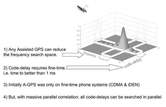
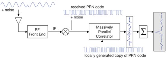
The cell-phone GPS revolution began with the catalyst of U.S. E911 legislation, which mandated that when an emergency (911) call is made from a cell phone, the location of the cell phone must be provided. Among several competing location technologies, GPS proved to be the big winner, thanks to seven technology enablers: assisted GPS, massive parallel correlation, high sensitivity, coarse-time navigation, low TOW, host-based GPS, and RF-CMOS.
All of these together enable very low-cost implementation of GPS in cell phones, even phones on networks such as GSM and W-CDMA that do not have fine-time synchronization (that is, they are not precisely synchronized with the GPS system). GPS is now found in roughly 500 million phones in use today.
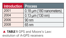
Four Milestones. From a consumer market perspective, we have exceeded forecasts. From a technology perspective, we have kept track with Moore’s law. Chips and receivers are cheaper than expected — because, as well as Moore’s law, we have seen greatly increased volumes and competition. Low-cost chips have not come at the expense of performance; in fact, the opposite — as chips have evolved, they have become less costly and better performing.
Small, cheap antennas have affected performance, but given the same antenna, I will demonstrate that a receiver with a single-die GPS chip costing less than $4 can outperform a $19,000 receiver.
This sounds paradoxical, even impossible — indeed many of you may be penning letters to the editor right now! But the time-to-first-fix, sensitivity, and urban-accuracy data will prove my point.
As a consequence of chip evolution, we are reaching plateaus of development for GPS-only systems. However, there remain many problems to solve, especially in urban canyons and indoors. These problems may never be solved with GPS alone, or with any single system alone. This decade will be characterized by GPS-plus; the days of GPS-only will soon recede into the past.
Don’t interpret this as a failing of GPS — quite the opposite. Because GPS-only systems have worked so well, they have found their way into half a billion cell phones, and we are boldly taking GPS to places no navigation has gone before. As we do, we start to encounter the limitations of GPS-only performance.
We will see the proliferation of GPS-plus: GPS+MEMS, GPS+Wi-Fi, GPS+NMR, and GPS+GLONASS, Compass, QZSS, and Galileo. The winners will be those with the greatest levels of integration. To paraphrase Winston Churchill, this is not the end of GPS, it is not even the beginning of the end. But it is, perhaps, the end of the beginning.
GNSS Consumer Market
For market forecasts made a few years ago, we can look at summaries provided in GNSS Markets and Applications, by Len Jacobson: a 2006 Frost & Sullivan report estimated the market for PNDs and handheld devices (not including cell phones) in 2010 would be $2.7 billion, with 8.3 million units, at an average selling price (ASP) of $325. In fact, this market today is approximately $6 billion, with 40 million units, at an ASP of $150.
Twice the Size. The consumer market, not including cell phones, is twice as big (in dollars) as forecast just a few years ago, even though prices are less than half forecast. Unit sales are more than four times forecast.
For the cell-phone market segment, in 1999 when the E911 rules were enacted in the United States, it was anticipated that A-GPS would be adopted only in fine-time (synchronized) networks, such as Verizon and Sprint CDMA. In coarse-time (non-synchronized) networks such as GSM, the expectation was that terrestrial wireless location techniques, such as time-difference-of-arrival (TDOA) and enhanced-offset-time-difference (E-OTD), would dominate. Today, only a few niches use TDOA, E-OTD is extinct, and GPS rules in coarse-time networks worldwide, including GSM in Europe and North America, and W-CDMA in Japan.
The consumer market, in particular the cell-phone market, has grown so rapidly that more receivers have been built in cell phones in the last three years than all other GPS built, ever. Today, L1 C/A-code GPS accounts for more than 99 percent of all GNSS receivers manufactured each year.
From a consumer market perspective, have we reached the point we expected to be by now?
Yes!
Not only have we arrived, we have far surpassed expectations.
GPS and Moore’s Law
Moore’s law says that for a given number of transistors, the chip size will halve every two years. Table 1 shows what this looks like in practice. For a particular class of GPS chip, the A-GPS receiver with massive parallel correlation, it shows release dates of different generations of these chips, and the technology process, which is the linear dimension of a single gate on the silicon die. As this dimension reduces to 70 percent of the previous value, the 2-dimensonal chip size reduces by 2 times. You can see Moore’s law in action here: approximately every two years, the technology process moves to the next level, and the chip size reduces by 2X. People are now talking about GPS chips in 45 nanometers, the next step.
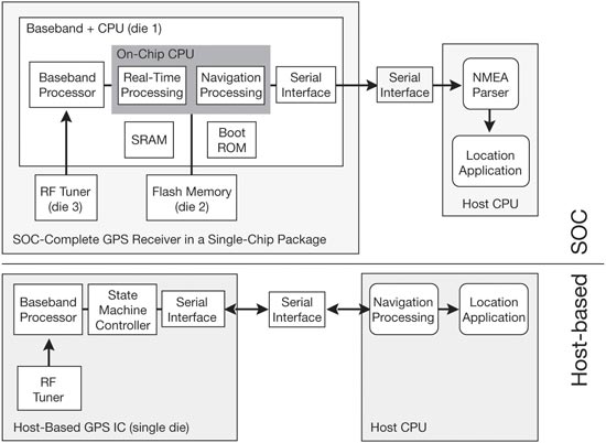
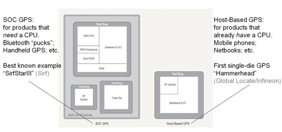
For a comparison, consider the Broadcom BCM 4751 chip, designed for cell phones. This chip is 2.9 X 3.1 millimeters, the size of the letter B on this page. This is a single-die host-based GPS/SBAS receiver, including RF front end, low-noise amplifier, baseband, and power management unit. Ten iterations of Moore’s law have passed in the last 20 years. The same chip, had it been built 20 years ago, would have been 210 times (a thousand times) bigger.
There were never chips that big. GPS chips aren’t just getting smaller with Moore’s law, they are getting vastly more complex and more capable.
Performance
At an elemental level, a GPS receiver does just three things: it starts, it tracks weak signals, and it computes position, velocity, and time. Strip away the obfuscating details, and performance may be summed up by: how fast, how sensitive, how accurate.
Since the 1990s, time to first fix ( TTFF) and sensitivity have improved dramatically, thanks to the seven technology enablers discussed earlier. TTFF for assisted cold starts, or unassisted warm starts, is now as good as one second, even without fine-time. This is a 45X improvement on typical GPS performance of the 1990s. Sensitivity increased roughly 30X (to -150 dBm) in 1998, then another 10X, (to -160 dBm) in 2006, and perhaps another three times to date, for a total of almost 1,000X extra sensitivity.
What about accuracy?
Some perceive low-cost chips as synonymous with low accuracy. This is not true. It is true that small, cheap antennas reduce accuracy; but given the same antennas, the lowest cost receivers on the market today will outperform the most expensive in typical environments where cell phones are used. The following figures show data to prove this point.
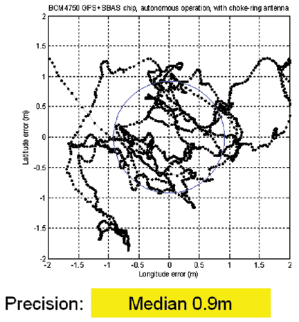
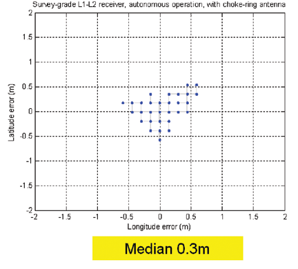
First we connect one of the smallest, lowest cost GPS receivers t
o one of the best antennas, a choke ring, on a rooftop with a clear view of the sky. Figure 1 shows the scatter of positions. The blue circle shows the median distribution, which is 0.9 meters for this dataset of 2000 fixes.
FIGURE 1a. Low-cost GPS with large, rooftop antenna.FIGURE 1b. Survey-grade GPS with large, rooftop antenna.
The adjacent plot shows the positions obtained from a $19,000 survey-grade GPS receiver, connected to the same antenna. The survey-grade GPS, with a median distribution of 0.3 meters, shows a 60-centimeter advantage over the cell-phone GPS, or maybe a 3X advantage depending on how you look at it. But don’t get too hung up on this result, because this is neither the typical consumer scenario (on a rooftop with choke-ring antenna), nor the main challenge facing us today.
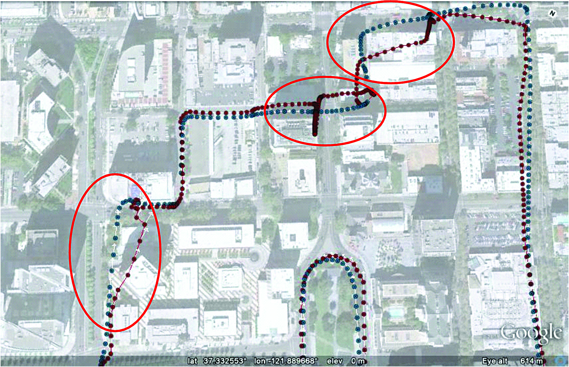
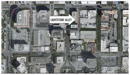
Next we look at the accuracy achieved with a more typical consumer antenna, in a more typical environment. Figure 2 shows the positions obtained in downtown San Jose with an active patch antenna, such as found in PNDs. San Jose is a fairly typical U.S. city, not the hardest place to use GPS, but not the easiest either. Lightstone Alley, adjacent to tall buildings, is only five meters wide.
FIGURE 2. Performance of cell-phone GPS (white) versus truth-reference system (blue). Median accuracy 4.4 meters, 67 percent 5.6 meters, 95 percent 11.2 meters.
To evaluate accuracy we used a truth-reference system combining GPS and a tactical-grade IMU with ring laser gyro to produce the blue dots on the figure. The white dots are the low-cost GPS positions. Most of the time, the white dots appear to be on top of the blue, but occasionally you see some separation, and there the red lines show the horizontal error. The median horizontal error is 4.4 meters.
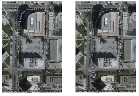
Figure 3 shows the comparison of low- and high-cost receivers, with the survey-grade receiver connected to the same patch antenna as the cell-phone GPS. There are many position gaps from the survey-grade receiver, and the position walks around when the vehicle is stationary (at the intersections, bottom left and top of the figure). This is because of the weak signals available in the urban environment. But don’t get too hung up on this result either, since we are still not at the real challenge of consumer GPS: location in severe urban canyons, such as San Francisco, New York, Chicago, Shanghai, Taipei, Shinjuku, and similar. In these, typically, only one or two GPS satellites can be seen directly. Other satellites may be tracked, but only by observing purely reflected signals. This is not classic GPS multipath, the combination of a direct and reflected signal; instead this is the combination of nothing but reflected signals. The direct signals are usually completely blocked by many buildings, and are not observable at all. So the whole premise of GPS — observing range from time of flight — breaks down, and it is very difficult to get good accuracy.
FIGURE 3. Comparison of cell-phone (left) and survey (right) receivers, both with patch antenna
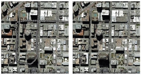
Figure 4 compares the cell-phone GPS with the survey-grade GPS, connected to the same small antenna, under such circumstances in San Francisco’s Financial District. There are no fixes at all from the survey-grade receiver. Why?
FIGURE 4. Cell-phone (left) and survey (right) receivers, in severe urban canyon
In Montgomery Street, there was only one directly visible satellite, with a signal strength of -132 dBm. All the other satellites were at -140 dBm or weaker, and traditional GPS receivers cannot acquire signals at this level. Hence the only receivers that work in this environment are modern high-sensitivity receivers most commonly found in cell phones.
You can see that the move to lower-cost receivers has not come at the expense of performance. In fact, the opposite: TTFF and sensitivity have improved dramatically, while accuracy has not been compromised, and is in fact much better in urban environments than legacy receivers, and even modern survey-grade receivers.
But are we there yet?
Although the consumer GPS market has irrefutably arrived, from a technical perspective the answer is more nuanced. Consumer GPS technology has made tremendous leaps forward. But precisely because of these improvements, we are taking GPS where it was never expected to go. It is no longer enough for GPS to work indoors (which it can). The demand is now for it to work as well as if it were outdoors (which, presently, it cannot).
Performance improvements seen with GPS-only will almost certainly not continue at the recent rate. We do not anticipate yet another 45X improvement in TTFF, or another 30 dB of sensitivity, for GPS alone. However, we do expect order-of-magnitude performance increases with the addition of other technologies. Figure 5 shows data from a TomTom 950, a GPS+MEMS containing the same GPS chip used in the earlier tests, MEMS accelerometers, and MEMS rate gyros. When tightly integrated and tested in the same deep urban canyons of San Francisco, the effect on position is good: median accuracy improved by 30 percent, worst-case errors are more than halved. But the result on heading accuracy is especially dramatic.
FIGURE 5. PND position accuracy (left), and heading accuracy (right), San Francisco
The bar graph shows the worst-case heading accuracy in each street. With GPS-only (red), the worst-case error is around 45 degrees, a familiar result to anyone who has used any GPS-only device in a similar environment: sooner or later the map will veer erroneously. However, with the integration of the MEMS rate gyros (blue), the worst-case heading errors drop to around 3 degrees, a 15X improvement in a key metric, similar to the improvements of the last decade, but now thanks to the effect of GPS-plus.
We will soon see GPS-plus many other technologies: Wi-Fi, NMR/MRL (power measurements from GSM and 3G phones), and of course GPS+GLONASS, Compass, QZSS, and Galileo. Because many mobile devices now include GPS, Wi-Fi, and 3G, there is a natural path for the evolution of GPS technology to include Wi-Fi and MRL measurements.
There is a also natural trend to source different radios from the same chip supplier. After all, why would you wish to undertake a do-it-yourself effort at removing co-existence issues in different radios, when a chip supplier has already done it for you?
Looking forward, it is very likely that this new decade will be characterized by GPS-plus other technologies, and the winners will be those with the greatest levels of integration.
Frank van Diggelen is senior technical director of GPS systems and chief navigation officer for Broadcom Corporation. He holds more than 45 U.S. patents, has a Ph.D. in electrical engineering from Cambridge University, and is the author of A-GPS: Assisted GPS, GNSS & SBAS.
Seven technologies that put GPS in mobile phones around the world — the how and why of location’s entry into modern consumer mobile communications.
By Frank van Diggelen, Broadcom Corporation
Exactly a decade has passed since the first major milestone of the GPS-mobile phone success story, the E-911 legislation enacted in 1999. Ensuing developments in that history include:
Snaptrack bought by Qualcomm in 2000 for $1 billion, and many other A-GPS startups are spawned.
Commercial GPS receiver sensitivity increases roughly 30 times, to 2150 dBm (1998), then another 10 times, to 2160 dBm in 2006, and perhaps another three times to date, for a total of almost 1,000 times extra sensitivity. We thought the main benefit of this would be indoor GPS, but perhaps even more importantly it has meant very, very cheap antennas in mobile phones. Meanwhile:
Host-based GPS became the norm, radically simplifying the GPS chip, so that, with the cheap antenna, the total bill of materials (BOM) cost for adding GPS to a phone is now just a few dollars!
Thus we see GPS penetration increasing in all mobile phones and, in particular, going towards 100 percent in smartphones.
This article covers the technology revolution behind GPS in mobile phones; but first, let’s take a brief look at the market growth. This montage gives a snapshot of 28 of the 228 distinct Global System for Mobile Communications (GSM) smartphone models (as of this writing) that carry GPS.
Back in 1999, there were no smartphones with GPS; five years later still fewer than 10 different models; and in the last few years that number has grown above 200. This is that rare thing, often predicted and promised, seldom seen: the hockey stick!
The catalyst was E-911 — abetted by seven different technology enablers, as well as the dominant spin-off technology (long-term orbits) that has taken this revolution beyond the cell phone.
In 1999, the Federal Communications Commission (FCC) adopted the E-911 rules that were also legislated by the U.S. Congress. Remember, however, that E-911 wasn’t all about GPS at first.
It was initially assumed that most of the location function would be network-based. Then, in September 1999, the FCC modified the rules for handset technologies. Even then, assisted GPS (A-GPS) was only adopted in the mobile networks synchronized to GPS time, namely code-division multiple access (CDMA) and integrated digital enhanced network (iDEN, a variant of time-division multiple access).
The largest networks in the world, GSM and now 3G, are not synchronized to GPS time, and, at first, this meant that other technologies (such as enhanced observed time difference, now extinct) would be the E-911 winners. As we all now know, GPS and GNSS are the big winners for handset location. E-911 became the major driver for GPS in the United States, and indirectly throughout the world, but only after GPS technology evolved far enough, thanks to the seven technologies I will now discuss.
Technology #1. Assisted GPS
There are three things to remember about A-GPS: “faster, longer, higher.” The Olympic motto is “faster, stronger, higher,” so just think of that, but remember “faster, longer, higher.”
The most obvious feature of A-GPS is that it replaces the orbit data transmitted by the satellite. A cell tower can transmit the same (or equivalent) data, and so the A-GPS receiver operates — faster.
The receiver has to search over a two-dimensional code/frequency space to find each GPS satellite signal in the first place. Assistance data reduces this search space, allowing the receiver to spend longer doing signal integration, and this in turn means higher sensitivity (Figure 1). Longer, higher.
FIGURE 1. A-GPS: reduced search space allows longer integration for higher sensitivity.
Now let’s look at this code/frequency search in more detail, and introduce the concepts of fine time, coarse time, and massive parallel correlation. Any assistance data helps reduce the frequency search. The frequency search is just as you might scan the dial on a car radio looking for a radio station — but the different GPS frequencies are affected by the satellite motion, their Doppler effect. If you know in advance whether the satellite is rising or setting, then you can narrow the frequency-search window.
The code-delay is more subtle. The entire C/A code repeats every millisecond. So narrowing the code-delay search space requires knowledge of GPS time to better than one millisecond, before you have acquired the signal. We call this “fine-time.”
Only two phone systems had this time accuracy: CDMA and iDEN, both synchronized to GPS time. The largest networks (GSM, and now 3G) are not synchronized to GPS time. They are within 62 seconds of GPS time; we call this “coarse-time.” Initially, only the two fine-time systems adopted A-GPS. Then came massive parallel correlation, technology number two, and high sensitivity, technology number three.
#2, #3. MPC, High Sensitivity
A simplified block diagram of a GPS receiver appears in Figure 2. Traditional GPS (prior to 1999) had just two or three correlators per channel. They would search the code-delay space until they found the signal, and then track the signal by keeping one correlator slightly ahead (early) and one slightly behind (late) the correlation peak. These are the so-called “early-late”correlators.
FIGURE 2. Massive parallel correllation.
Massive parallel correlation is defined as enough correlators to search all C/A code delays simultaneously on multiple channels. In hardware, this means tens of thousands of correlators. The effect of massive parallel correlation is that all code-delays are searched in parallel, so the receiver can spend longer integrating the signal whether or not fine-time is available.
So now we can be faster, longer, higher, regardless of the phone system on which we implement A-GPS.
Major milestones of massive parallel correlation (MPC):
In 1999, MPC was done in software, the most prominent example being by Snaptrack, who did this with a fast Fourier transform (FFT) running on a digital signal processor (DSP). The first chip with MPC in hardware was the GL16000, produced by Global Locate, then a small startup (now owned by Broadcom).
In 2005, the first smartphone implementation of MPC: the HP iPaq used the GL20000 GPS chip. Today MPC is standard on GPS chips found in mobile phones.
#4. Coarse-Time Navigation
We have seen that A-GPS assistance relieves the receiver from decoding orbit data (making it faster), and MPC means it can operate with coarse-time (longer, higher).
But the time-of-week (TOW) still needed to be decoded for the position computation and navigation: for unambiguous pseudoranges, and to know the time of transmission. Coarse-time navigation is a technique for solving for TOW, instead of decoding it. A key part of the technique involves adding an extra state to the standard navigation equation, and a corresponding extra column to the well known line-of-sight matrix.
The technical consequence of this technique is that you can get a position faster than it is possible to decode TOW (for example, in one, two, or three seconds), or you can get a position when the signals are too weak to decode TOW. And a practical consequence is longer battery life: since you can get fast time-to-first-fix (TTFF) always, without frequently waking and running the receiver to maintain it in a hot-start state.
#5. Low Time-of-Week
A parallel effort to coarse-time navigation is low TOW decode, that is, lowering the threshold at which
it is possible to decode the TOW data. In 1999, it was widely accepted that -142 dBm was the lower limit of signal strength at which you could decode TOW. This is because -142 dBm is where the energy in a single data bit is just observable if all you do is integrate for 20 ms.
However, there have evolved better and better ways of decoding the TOW message, so that now it can be done down to -152 dBm. Today, different manufacturers will quote you different levels for achievable TOW decode, anywhere from -142 to -152 dBm, depending on who you talk to. But they will all tell you that they are at the theoretical minimum!
#6, #7. Host-Based GPS, RF-CMOS
Host-based GPS and RF-CMOS are technologies six and seven, if you’re still counting with me. We can understand the host-based architecture best by starting with traditional system-on-chip (SOC) architecture. An SOC GPS may come in a single package, but inside that package you would find three separate die, three separate silicon chips packaged together: A baseband die, including the central processing unit (CPU); a separate radio frequency tuner; and flash memory. The only cost-effective way of avoiding the flash memory is to have read-only memory (ROM), which could be part of the baseband die — but that means you cannot update the receiver software and keep up with the technological developments we’ve been talking about. Hence state-of-the-art SOCs throughout the last decade, and to date, looked like Figure 3.
FIGURE 3. Host-based architecture, compared to SOC.
The host-based architecture, by contrast, needs no CPU in the GPS. Instead, GPS software runs on the CPU and flash memory already present on the host device (for example, the smartphone). Meanwhile, radio-frequency complementary metal-oxide semi-conductor (RF-CMOS) technology allowed the RF tuner to be implemented on the same die as the baseband. Host-based GPS and RF- CMOS together allowed us to make single die GPS chips.
The effect of this was that the cost of the chip went down dramatically without any loss in performance.
Figure 4 shows the relative scales of some of largest-selling SOC and host- based chips, to give a comparative idea of silicon size (and cost). The SOC chip (on the left) is typically found in devices that need a CPU, while the host-based chip is found in devices that already have a CPU.
FIGURE 4. Relative sizes of host-based, compared to SOC.
In 2005, the world’s first single-die GPS receiver appeared. Thanks to the single die, it had a very low bill of materials (BOM) cost, and has sold more than 50 million into major-brand smartphones and feature phones on the market.
Review
We have seen that E-911 was the big catalyst for getting GPS into phones, although initially only in CDMA and iDEN phones. E-911 became the driver for all phones once GPS evolved far enough, thanks to the seven technology enablers:
A-GPS >> faster, longer, higher
Massive parallel correlation >> longer, higher with coarse-time
High-sensitivity >> cheap antennas
Coarse time navigation >> fast TTFF without periodic wakeup
Low TOW >> decode from weak signals
Host-based GPS, together with
RF-CMOS g single die.
Meanwhile, as all this developed, several important spin-off technologies evolved to take this technology beyond the mobile phone. The most significant of all of these was long-term orbits (LTO), conceived on May 2, 2000, and now an industry standard.
Long-Term Orbits
Why May 2, 2000? Remember what happened on May 1, 2000: the U.S. government turned off selective availability (SA) on all GPS satellites. Suddenly it became much easier to predict future satellite orbits (and clocks) from the observations made by a civilian GPS network. At Global Locate, we had just such a network for doing A-GPS, as illustrated in Figure 5. On May 2 we said, “SA is off — wow! What does that mean for us?”And that’s where LTO for A-GPS came from.
FIGURE 5. Broadcast ephemeris and long-term orbits.
Figure 5 shows the A-GPS environment with and without LTO. The left half shows the situation with broadcast ephemeris only. An A-GPS reference station observes the broadcast ephemeris and provides it (or derived data) to the mobile A-GPS receiver in your mobile phone. The satellite has the orbits for many hours into the future; the problem is that you can’t get them.
The blue and yellow blocks in the diagram represent how the ephemeris is stored and transmitted by the GPS satellite. The current ephemeris (yellow) is transmitted; the future ephemeris (blue) is stored in the satellite memory until it becomes current. So, frustratingly, even though the future ephemeris exists, you cannot ordinarily get it from the GPS system itself.
The right half of the figure shows the situation with LTO. If a network of reference stations observes all the satellites all the time, then a server can compute the future orbits, and provide future ephemeris to any A-GPS receiver. Using the same color scheme as before, we show here that there are no unavailable future orbits; as soon as they are computed, they can be provided. And if the mobile device has a fast-enough CPU, it can compute future orbits itself, at least for the subset of satellites it has tracked.
Beyond Phones. This idea of LTO has moved A-GPS from the mobile phone into almost any GPS device. Two of most interesting examples are personal navigation devices (PNDs) in cars, and smartphones themselves that continue to be useful gadgets once they roam away from the network. Now, of course, people were predicting orbits before 2000 — all the way back to Newton and Kepler, in fact. It’s just that in the year 2000, accurate future GPS orbits weren’t available to mobile receivers. At that time, the International GNSS Service (IGS) had, as it does now, a global network of reference stations, and provided precise GPS orbits organized into groups called Final, Rapid and Ultra-Rapid. The Ultra-Rapid orbit had the least latency of the three, but, in 2000, Ultra-Rapid meant the recent past, not the future.
So for LTO we see that the last 10 years have taken us from a situation of nothing available to the mobile device, to today where these long-term orbits have become codified in the 3rd Generation Partnership Project (3GPP) and Secure User Plane Location (SUPL) wireless standards, where they are known as “ephemeris extension.”
Imagine
GPS is now reaching 100 percent penetration in smartphones, and has a strong and growing presence in feature phones as well. GPS is now in more than 300 million mobile phones, at the very least; credible estimates range above 500 million.
Now, imagine every receiver ever made since GPS was created 30 years ago: military and civilian, smart-bomb, boat, plane, hiking, survey, precision farming, GIS, Bluetooth-puck, personal digital assistant, and PND. In the last three years, we have put more GPS chips into mobile phones than the cumulative number of all other GPS receivers that have been built, ever!
Frank van Diggelen has worked on GPS, GLONASS, and A-GPS for Navsys, Ashtech, Magellan, Global Locate, and now as a senior technical director and chief navigation officer of Broadcom Corporation. He has a Ph.D. in electrical engineering from Cambridge University, holds more than 45 issued U.S. patents on A-GPS, and is the author of the textbook A-GPS: Assisted GPS, GNSS, and SBAS.
This update to a frequently requested article first published here in 1998 explains how statistical methods can create many different position accuracy measures. As the driving forces of positioning and navigation change from survey and precision guidance to location-based services, E911, and so on, some accuracy measures have fallen out of common usage, while others have blossomed. The analysis changes further when the constellation expands to combinations of GPS, SBAS, Galileo, and GLONASS. Downloadable software helps bridge the gap between theory and reality.
“There are three kinds of lies: lies, damn lies, and statistics.” So reportedly said Benjamin Disraeli, prime minister of Britain from 1874 to 1880. Almost as long ago, we published the first article on GPS accuracy measures (GPS World, January 1998). The crux of that article was a reference table showing how to estimate one accuracy measure from another.
The original article showed how to derive a table like TABLE 1. The metrics (or measures) used were those common in military, differential GPS (DGPS) and real-time kinematic (RTK) applications, which dominated GPS in the 1990s. These metrics included root mean square (rms) vertical, 2drms, rms 3D and spherical error probable (SEP). The article showed examples from DGPS data.
Table 1. Accuracy measures for circular, Gaussian, error distributions.Figure 1. Using Table 1.
Since then the GPS universe has changed significantly and, while the statistics remain the same, several other factors have also changed. Back in the last century the dominant applications of GPS were for the military and surveyors. Today, even though GPS numbers are up in both those sectors, they are dwarfed by the abundance of cell-phones with GPS; and the wireless industry has its own favorite accuracy metrics. Also, Selective Availability was active back in 1998, now it is gone. And finally we have the prospect of a 60+ satellite constellation, as we fully expect in the next nine years that 30 Galileo satellites will join the GPS and satellite-based augmentation systems (SBAS) satellites already in orbit.
Therefore, we take an updated look at GNSS accuracy.
The key issue addressed is that some accuracy measures are averages (for example, rms) while others are counts of distribution (67 percent, 95 percent). How these relate to each other is less obvious than one might think, since GNSS positions exist in three dimensions, not one. Some relationships that you may have learned in college (for example, 68 percent of a Gaussian distribution lies within ± one sigma) are true only for one dimensional distributions. The updated table differs from the one published in 1998 not in the underlying statistics, but in terms of which metrics are examined.
Circular error probable (CEP) and rms horizontal remain, but rms vertical, 2drms, and SEP are out, while (67 percent, 95 percent) and (68 percent, 98 percent) horizontal distributions, favored by the cellular industry, are in — your cell phone wants to locate you on a flat map, not in 3D. Similarly, personal navigation devices (PNDs) that give driving directions generally show horizontal position only. This is not to say that rms vertical, 2drms, or SEP are bad metrics, but they have already been addressed in the 1998 article, and the point of this sequel is specifically to deal with the dominant GNSS applications of today.
Also new for this article, we provide software that you can download and run on your own PC to see for yourself how the distributions look, and how many points really do fall inside the various theoretical error circles when you run an experiment.
Table 1 is the central feature of this article. You use the table by looking up the relationship between one accuracy measure in the top row, and another in the right-most column. For example (see FIGURE 1), let’s take the simplest entry in the table: rms2 = 1.41× rms1
TABLE 2 defines the accuracy measures used in this article.
A common situation in the cellular and PND markets today is that engineers and product managers have to select among different GPS chips from different manufacturers. (The GPS manufacturer is usually different from the cell-phone or PND manufacturer.) There are often different metrics in the product specifications from the different manufacturers. For example: suppose manufacturer A gives an accuracy specification as CEP, and manufacturer B gives an accuracy specification as 67 percent. How do you compare them? The answer is to use Table 1 to convert to a common metric. Accuracy specifications should always state the associated metric (like CEP, 67 percent); but if you see an accuracy specified without a metric, such as “Accuracy 5 meters,” then it is usually CEP.
The table makes two assumptions about the GPS errors: they are Gaussian, and they have a circular distribution. Let’s discuss both these assumptions.
Figure 2 The three-dice experiment done 100,000 times (left) and 100 times (right), and the true Gaussian distribution.
Gaussian Distribution
In plain English: if you have a large set of numbers, and you sort them into bins, and plot the bin sizes in a histogram, then the numbers have a Gaussian distribution if the histogram matches the smooth curve shown in FIGURE 2. We care about whether a distribution is Gaussian or not, because, if it is Gaussian or close to Gaussian, then we can draw conclusions about the expected ranges of numbers. In other words, we can create Table 1. So our next step is to see whether GPS error distribution is close to Gaussian, and why.
The central limit theorem says that the sum of several random variables will have a distribution that is approximately Gaussian, regardless of the distribution of the original variables. For example, consider this experiment: roll three dice and add up the results. Repeat this experiment many times. Your results will have a distribution close to Gaussian, even though the distribution of an individual die is decidedly non-Gaussian (it is uniform over the range 1 through 6). In fact, uniform distributions sum up to Gaussian very quickly.
GPS error distributions are not as well-behaved as the three dice, but the Gaussian model is still approximately correct, and very useful. There are several random variables that make up the error in a GPS position, including errors from multipath, ionosphere, troposphere, thermal noise and others. Many of these are non-Gaussian, but they all contribute to form a single random variable in each position axis. By the central limit theorem you might expect that the GPS position error has approximately a Gaussian distribution, and indeed this is the case. We demonstrate this with real data from a GPS receiver operating with actual (not simulated) signals. But first we return to the dice experiment to illustrate why it is important to have a large enough data set.
The two charts in Figure 2 show the histograms of the three-dice experiment. On the left we repeated the experiment 100,000 times. On the right we used just the first 100 repetitions. Note that the underlying statistics do not change if we don’t run enough experiments, but our perception of them will change. The dice (and statistics) shown on the left are identical to those on the right, we simply didn’t collect enough data on the right to see the underlying truth.
FIGURE 3 shows a GPS error distribution. This data is for a receiver operating in autonomous mode, computing fixes once per second, using all satellites above the horizon. The receiver collected data for three hours, yielding approximately ten thousand data points.
Figure 3. Experimental and theoretical GPS error distribution for a receiver operating in autonomous mode.
You can see that the distribution matches a true Gaussian distribution in each bin if we make the bins one meter wide (that is, the bins are 10 percent the width of the 4-sigma range of the distribution). Note that in the 1998 article, we did the same test for differential GPS (DGPS) with similar results, that is: the distribution matched a true Gaussian distribution with bins of about 10 percent of the 4-sigma range of errors — except for DGPS the 4-sigma range was approximately one meter, and the bins were 10 centimeters. Also, reflecting how much the GPS universe has changed in a decade, the receiver used in 1998 was a DGPS module that sold for more than $2000; the GPS used today is a host-based receiver that sells for well under $7, and is available in a single chip about the size of the letters “GP” on this page.
Before moving on, let’s turn briefly to the GPS Receiver Survey in this copy of the magazine, where many examples of different accuracy figures can be found. All manufacturers are asked to quote their receiver accuracy. Some give the associated metrics, and some do not. Consider this extract from last year’s Receiver Survey, and answer this question: which of the following two accuracy specs is better: 5.1m horiz 95 percent, or 4m CEP?
In Table 1 we see that CEP=0.48 × 95 percent. So 5.1 meters 95 percent is the same as 0.48× 5.1m = 2.4 meters CEP, which is better than 4 meters CEP.
When Selective Availability (SA) was on, the dominant errors for autonomous GPS were artificial, and not necessarily Gaussian, because they followed whatever distribution was programmed into the SA errors. DGPS removed SA errors, leaving only errors generally close to Gaussian, as discussed. Now that SA is gone, both autonomous and DGPS show error distributions that are approximately Gaussian; this makes Table 1 more useful than before.
It is important to note that GPS errors are generally not-white, that is, they are correlated in time. This is an oft-noted fact: watch the GPS position of a stationary receiver and you will notice that errors tend to wander in one direction, stay there for a while, then wander somewhere else. Not-white does not imply not-Gaussian. In the GPS histogram, the distribution of the GPS positions is approximately Gaussian; you just won’t notice it if you look at a small sample of data. Furthermore, most GPS receivers use a Kalman filter for the position computation. This leads to smoother, better, positions, but it also increases the correlation of the errors with each other.
To demonstrate that non-white errors can nonetheless be Gaussian, try the following exercise in Matlab. Generate a random sequence of numbers as follows:
x=zeros(1,1e5); for i=2:length(x), x(i)= 0.95*x(i-1)+0.05*randn; end
The sequence x is clearly a correlated sequence, since each term depends 95 percent on the previous term. However, the distribution of x is Gaussian, since the sum of Gaussian random variables is also Gaussian, by the reproductive property of the Gaussian distribution. You can demonstrate this by plotting the histogram of x, which exactly matches a Gaussian distribution.
In some data sets you may have persistent biases in the position. Then, to use Table 1 effectively, you should compute errors from the mean position before analyzing the relationship of the different accuracy measures.
Distributions and HDOP
Table 1 assumes a circular distribution. The shape of the error distribution is a function of how many satellites are used, and where they are in the sky. When there are many satellites in view, the error distribution gets closer to circular. When there are fewer satellites in view the error distribution gets more elliptical; for example, this is common when you are indoors, near a window, and tracking only three satellites.
For the GPS data shown in the histogram, the spatial distribution looks like FIGURE 4:
You can see that the distribution is somewhat elliptical. The rms North error is 2.1 meters, the rms East error is 1.2 meters. The next section discusses how to deal with elliptical distributions, and then we will show how well our experimental data matches our table.
Figure 4. Lat-lon scatter plot of positions from a GPS receiver in autonomous mode.
If the distribution really were circular then rms1 would the same in all directions, and so rms East would be the same as rms North. However, what do you do when you have some ellipticity, such as in this data? The answer is to work with rms2 as the entry point to the table. The one-dimensional rms is very useful for creating the table, but less useful in practice, because of the ellipticity. Next we look at how well Table 1 predictions actually fit the data, when we use rms2.
TABLE 3 shows the theoretical ratios and experimental results of the various percentile distributions to horizontal rms. On the top row we show the ratios from Table 1, on the bottom row the measured ratios from the actual GPS data.
Table 3. Theoretical ratios and experimental results using actual GPS data.
For our data: horizontal rms = rms2 = 2.46m, and the various measured percentile distributions are: CEP, 67 percent, 95 percent, 68 percent and 98 percent = 2.11, 2.62, 4.15, 2.65, and 4.74m respectively.
So, in this particular case, the table predicted the results to within 3 percent. With larger ellipticity you can expect the table to give worse results. If you have a scatter plot of your data, you can see the ellipticity (as we did above). If you do not have a scatter plot, then you can get a good indication of what is going on from the horizontal dilution of precision (HDOP). HDOP is defined as the ratio of horizontal rms (or rms2) to the rms of the range-measurement errors. If HDOP doubles, your position accuracy will get twice as bad, and so on. Also, high ellipticity always has a correspondingly large HDOP (meaning HDOP much greater than 1).
Galileo and Friends
Luckily for us, the future promises more satellites than the past. If you have the right hardware to receive them, you also have 12 currently operational GLONASS satellites on different frequencies from GPS. Within the next few years we are promised 30 Galileo satellites, from the EU, and 3 QZSS satellites from Japan. All of these will transmit on the same L1 frequency as GPS. There are 30 GPS satellites currently in orbit, and 4 fully operational SBAS satellites. Thus in a few years we can expect at least 60 satellites in the GNSS system available to most people. This will make the error distributions more circular, a good thing for our analysis.
Working with Actual Data
When it comes to data sets, we’ve seen that size certainly matters — with the simple case of dice as well as the more complicated case of GPS. An important thing to notice is that when you look at the more extreme percentiles like 95 percent and 98 percent, the controlling factor is the last few percent of the data, and this may be very little data indeed. Consider an example of 100 GPS fixes. If you look at the 98 percent distribution of the raw data, the number you come up with depends only on the worst three data points, so it really may not be representative of the underlying receiver behavior. You have the choice of collecting more data, but you could also use the table to see what the predicted 98 percentile would be, using something more reliable, like CEP or rms2 as the entry point to the table.
Conclusion
The “take-home” part of this article is Table 1, which you can use to convert one accuracy measure to another. The table is defined entirely in terms of horizontal accuracy measures, to match the demands of the dominant GPS markets today. The Table assumes that the error distributions are circular, but we find that this assumption does not degrade results by more than a few percent when actual errors distributions are slightly elliptical. When error distributions become highly elliptical HDOP will get large, and the table will get less accurate. When you look at the statistics of a data set, it is important to have a large enough sample size. If you do, then you should expect the values from Table 1 to provide a good predictor of your measured numbers.
Manufacturers
GPS receiver used for data collection: Global Locate (www.globallocate.com) Hammerhead single-chip host-based GPS.
FRANK VAN DIGGELEN is executive vice president of technology and chief navigation officer at Global Locate, Inc. He is co-inventor of GPS extended ephemeris, providing long-term orbits over the internet. For this and other GPS inventions he holds more than 30 US patents. He has a Ph.D. E.E. from Cambridge University.