Tag: Innovation

  • Innovation: A look back at 35 Years of ‘Innovation’

    Innovation: A look back at 35 Years of ‘Innovation’

    Innovation Insights with Richard Langley
    Innovation Insights with Richard Langley

    Click to read the full Innovation Insights column, Innovation Insights: It starts with the physics”

    This is my 300th and last “Innovation” column in GPS World. I have mixed feelings about stopping the column. I’ve really enjoyed doing it for the past 35 years, but editorial deadlines can be difficult to meet sometimes, especially when I’ve got other things to get done or if they come in the middle of a vacation.

    To rephrase the old adage, editorial deadlines wait for no one. Looking back, I don’t know how I managed to initially produce six and then 10 columns each year, along with all my other duties as a university professor. Mind you, as I’ll soon discuss, most of the articles in the columns were authored by others. My job mostly was to edit the articles to help the authors tell their stories in a particular GPS World style and sometimes to improve their submitted figures. Additionally, in 2006, I started to write a sidebar called “Insights” to provide some basic background material about each column’s topic. A few years ago, I became editor-in-chief of the Institute of Navigation’s journal NAVIGATION, which takes up a bit of my time, along with lecturing and managing a research team. So, at 75, I thought it might be a good time to lessen the load a little bit.

    In this last column, I’m going to tell the story of how “Innovation” came to be and review some of the column’s developments over the years.

    How it all began

    In the fall of 1989, GPS World’s founding editor, Glen Gibbons, approached Dave Wells, Ph.D., a fellow faculty member in the then Department of Surveying Engineering at the University of New Brunswick (UNB) – about assisting with a “technology/product development column” in the magazine he was about to start. Glen wanted it to provide “an analysis and commentary on the research, development, product issues and needs of the GPS community.” And, since GPS World readers would have marked differences in their knowledge and expertise in the GPS area, “the column should deal with issues that have broad application and interest and are presented in terms that are accessible to as wide a range of readers as possible,” Glen said in a letter to Dave.

    Glen had heard about Dave’s (and UNB’s) early involvement with GPS. When I came to UNB in 1981, UNB was already carrying out some of the first theoretical studies on how GPS could be used by surveyors and geodesists for precise positioning. Shortly afterwards, UNB participated in some of the first surveys using the Macrometer V-1000 and Texas Instruments TI 4100 receivers and developed software to process the resulting data. In 1983, Dr. Gerhard Beutler from the Astronomical Institute of the University of Bern came to UNB on a sabbatical and began developing his own GPS data processing software that would eventually become the Bernese GNSS Software or just “Bernese” to those in the know. Somehow, in between our GPS algorithm and software development, teaching, mentoring graduate students and other duties, we managed to self-publish the first textbook on GPS, Guide to GPS Positioning. With a publication date of December 31, 1986, it went on to sell more than 12,000 copies in the English version alone. It was also translated into Chinese, Spanish and Vietnamese. So, perhaps it is not surprising that Glen came to knock on UNB’s door when he was starting up his magazine.

    Getting back to Glen’s letter, he went on to say, “It would be possible to handle the preparation or presentation of the column in one of several ways: We could identify a single person who would have primary responsibility for writing all the columns and whose byline would appear on them; we could have a person act as the coordinating editor responsible for obtaining suitable contributions from various authors; or we could establish a collective or institutional editorship with column responsibilities shared among a pool of contributors.”

    The letter arrived in early November 1989, and Dave, I and Alfred Kleusberg, Ph.D., who was a research fellow in the department (and subsequently a professor), began to discuss whether we wanted to take on the responsibility for the column and, if so, how we would manage it. I shortly departed to the University of Bern, where I would spend the better part of two months during my first sabbatical. Communication had to take place using e-mail, although phone, telefax and telex were also possible. Universities had e-mail before most other organizations thanks to BITNET (known initially in Europe as the European Academic and Research Network or EARN), a computer network that predated the Internet. My BITNET e-mail address was lang@unb or [email protected]. As I recall, the personal part of the address was limited to at most four characters. So, when UNB joined the Internet, I basically kept the same e-mail address: [email protected]. I talked about GPS and the Internet in the November 1995 edition of the column. But I’m getting ahead of myself.

    FIGURE 1: First page of Dave Wells’ notes from December 31, 1989 on how UNB would manage the “Innovation” column. (Photo: GPS World archives)
    FIGURE 1: First page of Dave Wells’ notes from December 31, 1989 on how UNB would manage the “Innovation” column. (Photo: GPS World archives)

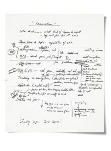
    That December, the three of us more or less agreed that we would handle the column in some form. From Switzerland, I sent Dave a list of 12 possible topics for the column, but I added the rider: “Note that I am not necessarily volunteering to write any of the articles.” As we know, things turned out a little differently. During the university’s Christmas break, after I returned to Fredericton, we met at Dave’s house to discuss how we would manage the column in more detail. We met on New Year’s Eve — a Sunday afternoon — and decided that Alfred Kleusberg and I would manage the column as co-editors, with Dave serving as one of the inaugural members of the magazine’s Editorial Advisory Board. The column editorship was to be a blend of the second and third of Glen’s suggestions. The task wasn’t supposed to be too onerous. After all, the magazine was to be published bimonthly. Lots of time to get someone to write an article and for Alfred and I to edit it. Or so we thought. And the column was to be called, simply, “Innovation.” I don’t recall who came up with the name — whether it was one of the three of us or Glen, but the notes from that Sunday afternoon meeting have “Innovation” written at the top of the first page (see FIGURE 1). Ideally, as per Glen’s suggested guidelines, column articles were to be tutorial in style or written in a way that they could be understood, for the most part, by non-experts in the field.

    At that Sunday afternoon meeting, we decided that Dave and Alfred would write the article for the first column. It was an introduction to GPS and some possible applications titled “GPS: A Multipurpose System.” With a couple of iterations of the article back and forth with Glen via fax (GPS World didn’t have e-mail until a few years later) and a figure delivery by FedEx, the column debuted in GPS World, Volume 1, Issue 1, January/February 1990.

    It used three different positioning scenarios to explain how GPS could provide positioning accuracies from a Selective Availability-constrained 100 meters down to the sub-centimeter level. It also outlined GPS’s ability to determine platform attitude with multiple antennas and its use for accurate time transfer.
    There was a brief introductory couple of paragraphs, which would be a column standard (later extended to a sidebar). That first introduction went as follows:

    “‘Innovation’ will be a regular column in GPS World and will comment on GPS technology, product development, and other issues and needs of the GPS community. Coordinating editors are Alfred Kleusberg, Ph.D. and Richard Langley, Ph.D. both of the Department of Surveying Engineering at the University of New Brunswick in Fredericton, New Brunswick, Canada, as is David Wells, Ph.D., co-author of this initial column.

    “The first few columns will introduce GPS World readers to GPS technology. This first column focuses on the many capabilities of GPS. The next column will look at the flip side — what are the limitations of GPS? ‘Innovation’ will discuss some intriguing questions in future columns: Why is the GPS signal so complicated? How have surveyors been able to use it to get such accurate results? How serious is selective availability? We will also devote columns to exploring in depth some of the issues raised in this column: GPS and electronic charts, GPS and geographical information systems and prospects for using GPS and GLONASS together. We welcome readers’ comments and topic suggestions for future columns.”

    That introduction listed the topics for the first year of “Innovation.” They were written by Alfred, me, both of us, or other researchers at UNB and, in one case, by colleagues at the Canadian Hydrographic Service. We had a very positive response to our first few column articles, so Glen kept us on, but at some point in 1990, he told us the magazine was going to 10 issues a year. There were just too many GPS-related developments to be covered in just six issues. So now there would be a monthly column except for the July/August and November/December issues.

    In the second year, Alfred and I continued to write some tutorial articles for the column, but we started to invite others to submit articles, which we would then edit for style and space, and that became the tradition. Over the years, we have had hundreds of leaders in GNSS technology development and applications pen articles. In the second and third years of the column, for example, we featured articles by Stephen DeLoach on precise real-time dredge positioning, Jack Klobuchar on ionospheric effects on GPS, Edward Krakiwsky on GPS vehicle location and navigation, Yehuda Bock on continuous monitoring of crustal deformation, Keith D. McDonald on GPS in civil aviation, David Coco on GPS as satellites of opportunity for ionospheric monitoring, Derrick Peyton on using GPS and remotely-operated vehicles to map the ocean, Oscar Colombo and Mary Peters on precision long-range DGPS for airborne surveys, Adam Freedman on measuring the Earth’s rotation and orientation with GPS, Christian Rocken and Thomas Kelecy on high-accuracy GPS marine positioning for scientific applications, Marvin May on measuring velocity using GPS, Thomas Yunck describing a new chapter in precise orbit determination, and Gregory Leger on using GPS-equipped drift buoys for search and rescue operations. And the list goes on and on.

    As I mentioned, in the second year of GPS World, there were 10 issues. That changed in 1993, when the magazine went to 12 issues a year, but the September and December issues were “Showcase” issues featuring more industrial news and announcements of new products. It was also to include “The Almanac” — an update on the GNSS constellations, which I also looked after. Eventually, the “Showcase” issues became regular issues but with “Innovation” replaced by “The Almanac” at the “back of the book.”

    Figure 2A Different eras of “Innovation” throughout the years; the January 1993 edition (left) and the January 2000 edition (right). (Photo: GPS World archives)
    Figure 2A Different eras of “Innovation” throughout the years; the January 1993 edition (left) and the January 2000 edition (right). (Photo: GPS World archives)

    The column look changed a few times over the years, typically coinciding with magazine makeovers, with the logo changing from the original 3D terrain graphic to a logo of people with stuff in their hands starting in January 1999, to a “bits” logo from January 2001, to a somewhat plain format from September 2003, with the “Insights” sidebar and my photo from April 2006, to a circle photo from November 2015, and with a new photo from January 2016. FIGURES 2A, 2B and 2C show representative column snapshots for each era.

    Figure 2B Different eras of “Innovation” throughout the years; the January 2003 edition (left) and the September 2003 edition (right). (Photo: GPS World archives)
    Figure 2B Different eras of “Innovation” throughout the years; the January 2003 edition (left) and the September 2003 edition (right). (Photo: GPS World archives)


    FIGURE 2c  Different eras of “Innovation” throughout the years; the April 2006 edition (left) and the February 2016 edition (right). (Photo: GPS World archives)
    FIGURE 2c Different eras of “Innovation” throughout the years; the April 2006 edition (left) and the February 2016 edition (right). (Photo: GPS World archives)

    The tutorials

    As I mentioned earlier, right from the beginning of “Innovation,” we decided to have essentially two types of articles in the column: discussions of recent advances in GPS (and later GNSS) applications and related technology written by guest authors and tutorials explaining the fundamentals of GNSS including how the three main components of GNSS work: the satellites, the control segment and the user equipment. Here is a list of some of the tutorials written by the UNB team (mostly me) that were featured in “Innovation”:

    • GPS: A Multipurpose System (January/February 1990)
    • The Limitations of GPS (March/April 1990)
    • Why is the GPS Signal So Complex? (May/June 1990)
    • The Issue of Selective Availability (Sept./Oct. 1990)
    • Comparing GPS and GLONASS (Nov./Dec. 1990)
    • The GPS Receiver: An Introduction (Jan. 1991)
    • The Orbits of GPS Satellites (March 1991)
    • The Mathematics of GPS (July/August 1991)
    • Time, Clocks, and GPS (Nov./Dec. 1991)
    • Basic Geodesy for GPS (February 1992)
    • The Federal Radionavigation Plan (March 1992)
    • Precise Differential Positioning and Surveying (July 1992)
    • The GPS Observables (April 1993)
    • Communication Links for GPS (May 1993)
    • GPS and the Measurement of gravity (Oct. 1993)
    • RTCM SC-104 DGPS Standards (May 1994)
    • NMEA 0183: A GPS Receiver Interface Standard (July 1995)
    • Mathematics of Attitude Determination with GPS (Sept. 1995)
    • A GPS Glossary (Oct. 1995)
    • GPS and the Internet (Nov. 1995)
    • The GPS User’s Bookshelf (Jan. 1996)
    • Coordinates and Datums and Maps! Oh My! (with Will Featherstone; Jan. 1997)
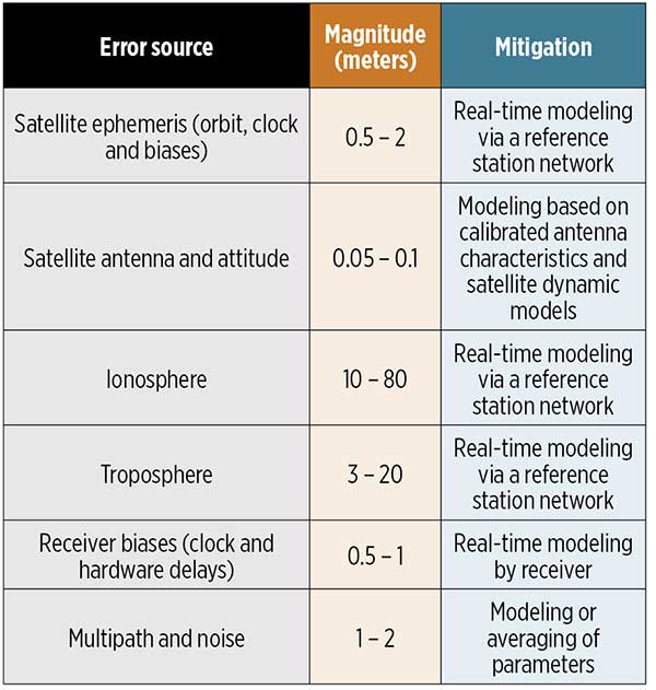
    • The GPS Error Budget (March 1997)
    • GPS Receiver System Noise (June 1997)
    • GLONASS: Review and Update (July 1997)
    • The UTM Grid System (Feb. 1998)
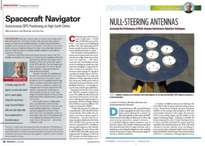
    • A Primer on GPS Antennas (July 1998)
    • RTK GPS (September 1998)
    • The GPS End-of-Week Rollover (Nov. 1998)
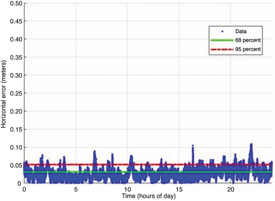
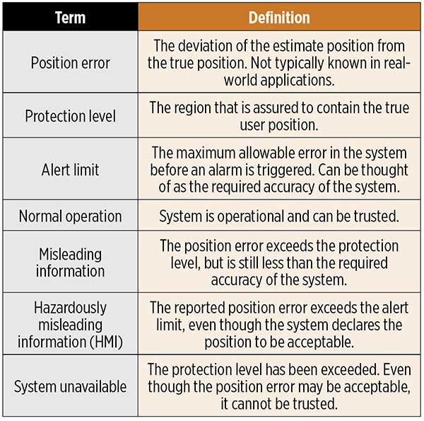
    • The Integrity of GPS (March 1999)
    • Dilution of Precision (May 1999)
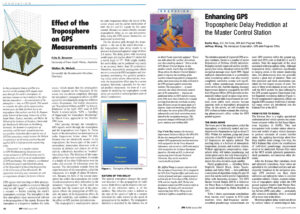
    • GPS, the Ionosphere, and the Solar Maximum (July 2000)
    • Navigation 101: Basic Navigation with a GPS Receiver (October 2000)
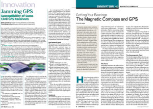
    • Getting Your Bearings: The Magnetic Compass and GPS (Sept. 2003)
    • GPS by the Numbers: A Sideways Look at How the Global Positioning System Works (April 2010); this was the 200th “Innovation” column.

    As you can see, the tutorials became fewer as the years went by. As my research career expanded, I just didn’t have the additional time to write more tutorials. I had taken over sole responsibility for the column in 1997, shortly after Alfred Kleusberg left UNB to pursue a career opportunity in Germany.

    However, the tutorial columns were (and still are) popular judging by the comments sent to GPS World and the number of citations for some reported by Google Scholar. For example, the one on dilution of precision has been cited in papers, theses, and reports 837 times to date. While not as many as a paper on an important medical breakthrough, it’s not a bad record for an article on a navigation topic.

    Changes at the top

    The column has seen four changes of editorial leadership at GPS World. Glen Gibbons, the founding editor, stepped down as editor-in-chief in July 2005 and shortly afterward started up his own publishing company to produce the magazine Inside GNSS. Alan Cameron took over the job in 2006, and subsequently became the magazine’s publisher and editor-at-large. Tracy Cozzens became the senior editor in 2019 with responsibility for “Innovation,” and then Matteo Luccio became editor-in-chief of the magazine in May 2021. I’m happy to say I got along well with all of these “bosses,” and they continued to put up with me even when I got the column in at the last moment. Additionally, the magazine’s various art directors over the years have always made the column look good.

    However, after I took over sole responsibility for the column, there were no changes at the bottom. So, I’ve ended up being the longest serving GNSS rapporteur or editor, with Glen and Alan and Tracy having retired at different epochs during the past decade. In addition to the column, I have contributed a number of shorter articles to the magazine and the GPS World website over the years, sometimes joined by colleagues from different organizations, in particular the German Aerospace Center.

    A bit of my own history

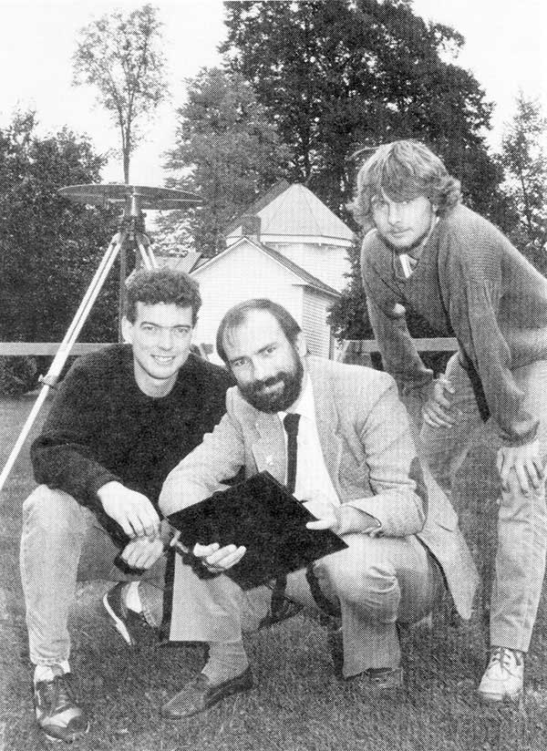
    I wasn’t going to bother with an “Insights” sidebar for this last column. The column isn’t about a single topic that needs any background information. But you might be wondering how I got this gig as the “Innovation” editor (apart from what I’ve already told you) or got my job at UNB for that matter. So, I’m repurposing the “Insights” sidebar from the February 2016 issue of GPS World, in which I talk a bit about antenna arrays and my own radio tinkering. It doesn’t mention that after getting my Ph.D., I spent two years at MIT as a postdoctoral fellow working under the famous physicist Irwin Shapiro on analyzing lunar laser ranging data to uncover subtle changes in Earth’s rotation due to the fluctuating winds of its atmosphere. Even as a graduate student, I was involved with satellite navigation and helped to uncover a bias in the coordinate system used by the U.S. Navy Navigation Satellite System, commonly known as Transit, by comparing station coordinates with those I obtained in my very long baseline interferometry research. I’ve always been a radio nerd both in my day job and as an avid shortwave radio hobbyist. So, it is not too surprising that I got involved with GPS and then GNSS (including ionospheric studies) and established a GNSS research group at UNB with some stellar graduates over the years.

    The archives

    I would like to report that all 300 “Innovation” columns are available for download on the Internet. Unfortunately, that is not the case — yet. Perhaps that’s something that could be done when I actually do retire. However, the first two years of the column are available here: gauss.gge.unb.ca/gpsworld/innovation.html. Hopefully, we can continue to keep that URL alive for a few years. If it should disappear, just Google it or consult the “Wayback Machine” at archive.org. The columns since June 2008 (with a few more before that) are available here. Full digital versions of each issue of the magazine since January 2009, including the “Innovation” column, are available here.

    The end

    And there you have it. It only remains for me to thank all of the authors who have shared their research and understanding of the many facets of GNSS in the column over the past three-and-a-half decades, the staff at GPS World for getting the column into the print and later the electronic editions on the Web, the readers whose positive feedback encouraged me to keep the column going, and to my wife, Marg, who let me spend the long hours on the column when I should have been attending to things around the house. So, now, to paraphrase a much better journalist than I: Goodbye, and good luck.


    The November 2024 issue of GPS World features Professor Richard Langley’s 300th and final “Innovation” column. His first one appeared in the January/February 1990 issue, the magazine’s very first. In celebration of Richard’s decades-long contribution to GPS / GNSS / PNT, we are publishing a selection of testimonials and photos from some of his colleagues and friends, gathered by his former students Sunil Bisnath and Attila Komjathy. Click here to read the testimonials.

  • GNSS Spoofing Detection: Guard against automated ground vehicle attacks

    GNSS Spoofing Detection: Guard against automated ground vehicle attacks

    Read Richard Langley’s introduction column, Innovation Insights: What is a carrier phase?


    An approach for ground vehicles using carrier-phase and inertial measurement data

    The combination of easily accessible low-cost GNSS spoofers and the emergence of increasingly automated GNSS-reliant ground vehicles prompts a need for fast and reliable GNSS spoofing detection. To underscore this point, Regulus Cyber, an Israeli cybersecurity company, recently spoofed a Tesla Model 3 on autopilot mode, causing the vehicle to suddenly slow and unexpectedly veer off the main road.

    Among GNSS signal authentication techniques, signal-quality monitoring (SQM) and multi-antenna could be considered for implementation on ground vehicles. However, SQM tends to perform poorly on dynamic platforms in urban areas where strong multipath and in-band noise are common, and multi-antenna spoofing detection techniques, while effective, are disfavored by automotive manufacturers seeking to reduce vehicle cost and aerodynamic drag. Thus, there is a need for a single-antenna GNSS spoofing detection technique that performs well on ground vehicles, despite the adverse signal-propagation conditions in an urban environment.

    In a concurrent trend, increasingly automated ground vehicles demand ever-stricter lateral positioning to ensure safety of operation. An influential study calls for lateral positioning better than 20 centimeters on freeways and better than 10 centimeters on local streets (both at a 95% probability level). Such stringent requirements can be met by referencing lidar and camera measurements to a local high-definition map, but poor weather (heavy rain, dense fog or snowy whiteout) can render this technique unavailable.

    On the other hand, progress in precise (decimeter-level) GNSS-based ground vehicle positioning, which is impervious to poor weather, has demonstrated surprisingly high (above 97%) solution availability in urban areas. This technique is based on carrier-phase differential GNSS (CDGNSS) positioning, which exploits GNSS carrier-phase measurements having millimeter-level precision but integer-wavelength ambiguities.

    Key to our promising results is the tight coupling of CDGNSS and inertial measurement unit (IMU) data, without which high-accuracy CDGNSS solution availability is significantly reduced due to pervasive signal blockage and multipath in urban areas. Tight coupling brings millimeter-precise GNSS carrier-phase measurements into correspondence with high-sensitivity and high-frequency inertial sensing. Our particular estimation architecture incorporates inertial sensing via model replacement, in which the estimator’s propagation step relies on bias-compensated acceleration and angular rate measurements from the IMU instead of a vehicle dynamics model.

    As a consequence, at each measurement update, an a priori antenna position is available whose delta from the previous measurement update accounts for all vehicle motion sensed by the IMU, including small-amplitude high-frequency motion caused by road irregularities. Remarkably, when tracking authentic GNSS signals in a clean (open-sky) environment, the GNSS carrier-phase predicted by the a priori antenna position and the actual measured carrier phase agree to within millimeters.

    The research described in this article pursues a novel GNSS spoofing-detection technique based on a simple but consequential observation: it is practically impossible for a spoofer to create a false ensemble of GNSS signals whose carrier-phase variations, when received through the antenna of a target ground vehicle, track the phase values predicted by inertial sensing. In other words, antenna motion caused by factors such as road irregularities or rapid braking or steering is sensed with high fidelity by an onboard IMU but is unpredictable at the sub-centimeter-level by a would-be spoofer.

    Therefore, the differences between IMU-predicted and measured carrier-phase values offer the basis for an exquisitely sensitive GNSS spoofing-detection statistic. What is more, such carrier-phase fixed-ambiguity residual cost is generated as a byproduct of tightly coupled inertial-CDGNSS vehicle position estimation.

    Two difficulties complicate the use of fixed-ambiguity residual cost for spoofing detection. First is the integer-ambiguous nature of the carrier-phase measurement, which causes the post-integer-fix residual cost to equal not the difference between the measured and predicted carrier phases (as would be the case for a typical residual), but rather modulo an integer number of carrier wavelengths. Such integer folding complicates development of a probability distribution for a detection test statistic based on carrier-phase fixed-ambiguity residual cost.

    Second, the severe signal multipath conditions in urban areas create thick tails in any detection statistic based on carrier-phase measurements. Setting a detection threshold high enough to avoid false spoofing alarms caused by mere multipath could render the detection test insensitive to dangerous forms of spoofing. Reducing false alarms by accurately modeling the effect of a particular urban multipath environment on the detection statistic would be a Sisyphean undertaking, requiring exceptionally accurate up-to-date 3D models of the urban landscape, including materials properties.

    Our work takes an empirical approach to these difficulties. It does not attempt to develop a theoretical model to delineate the effects of integer folding or multipath on its proposed carrier-phase fixed-ambiguity residual cost-based detection statistic. Rather, it develops null-hypothesis empirical distributions for the statistic in both shallow and deep urban areas, and uses these distributions to demonstrate that high-sensitivity spoofing detection is possible despite integer folding and urban multipath.

  • Innovation Insights: What is carrier phase?

    Innovation Insights: What is carrier phase?

    Innovation Insights with Richard Langley
    Innovation Insights with Richard Langley

    WHAT IS CARRIER PHASE? The obvious answer is: the phase of the carrier. But this is not helpful if you don’t know what a carrier is. A carrier is basically a harmonic electromagnetic wave — a pure continuous sinusoidal wave with a single constant frequency and amplitude.

    Such a wave has limited uses. However, if we modulate or change the characteristics of the wave in some way, then the wave can carry information. Changing the amplitude by using a voice or music audio signal is amplitude modulation as used for AM radio.

    Instead, one could modulate a carrier by changing its instantaneous frequency, which is frequency modulation or FM and is used for high-fidelity broadcasting. Yet another way to modulate a carrier is to change the instantaneous phase of the carrier, and that is how GNSS works.

    GNSS carriers are phase-modulated by pseudorandom noise (PRN) codes and navigation messages. A GNSS receiver uses the PRN codes to produce the pseudorange observable with a precision in the tens of decimeter range. This is the most common observable for GNSS positioning.

    But by stripping away the modulation of the received GNSS signals, the receiver can measure the phase of the underlying carrier. Changes in carrier phase over time reflect the change in the (pseudo)range but are about two orders of magnitude more precise.

    One problem with carrier-phase measurements is that they have an initial cycle ambiguity that must be resolved, preferentially fixed to the correct integer value, before they can be used for positioning, but this can be achieved without too much difficulty. While fixing the ambiguity of carrier-phase measurements might be considered a nuisance in GNSS positioning, it can help detect spoofing of GNSS signals where some other techniques might fall short.

    In this “Innovation” column, we look at how carrier-phase measurements combined with those from an inertial measurement unit can guard against a deliberate attack on an automated ground vehicle — something that cannot be discounted in our world these days.

    Read the full “Innovation” column: GNSS Spoofing Detection: Guard against automated ground vehicle attacks.

  • Innovation: Software-defined radios for GNSS

    Innovation: Software-defined radios for GNSS

    A Step-by-Step Exposition of an Educational Resource

    Innovation Insights with Richard Langley
    Innovation Insights with Richard Langley

    THE RADIO. It’s been around for more than 100 years. Pioneering work by Guglielmo Marconi and others in the1890s and 1900s resulted in practical wireless telegraphy devices that permitted point-to-point communications with ships at sea and between stations on land hundreds and thousands of kilometers apart and even between stations on different continents. The first radio broadcasts (point-to-multipoint) were time signal transmissions and weather broadcasts. Experimental audio transmissions took place in the early 1900s, and by 1920 or so, radio stations were established in many countries for broadcasting speech and music to the general public.

    The first radio receivers were simple crystal sets. It wasn’t until the mid-1920s that tube radios became commercially available. Eventually, tubes were replaced by transistors, and transistors by integrated circuits. The introduction of microprocessors resulted in digital receivers, with the conversion of the received analog radio signals into audio being carried out digitally for the most part.
    One of the latest advances in radio technology is the software-defined radio or SDR. An SDR typically consists of two components: a piece of hardware, called a radio frequency (RF) front end, and a piece of software run on a general-purpose computer. The job of the front end is to convert a portion of the radio spectrum received by its antenna to a digital data stream processed by the software. The software decodes the data to produce the desired result. Since the software does most of the “heavy lifting” in processing a radio signal, it is often called the SDR itself. And by the way, there are SDR transmitters, too.

    It should come as no surprise that SDR technology has come to the GNSS field. In fact, in 2007, the seminal text on GNSS SDRs, A Software-Defined GPS and Galileo Receiver: A Single-Frequency Approach, was published along with the sale of an inexpensive RF front-end in a thumb-drive-sized package that allowed graduate students and others to experiment with a GNSS SDR themselves. And we have covered GNSS SDR developments in this column from time to time, most recently in January 2018 (“The Continued Evolution of the GNSS Software-Defined Radio: Getting Better All the Time”).

    In this month’s column, researchers from the lab that helped produce the SDRs documented in the 2007 book (which is still in print) discuss their development and testing of additional freely available SDR codebases covering all four GNSS (GPS, Galileo, BeiDou and GLONASS). They provide an excellent resource for learning how GNSS receivers actually work.


    By Joan Bernabeu, Nicolas Gault, Yafeng Li and Dennis M. Akos

    With the publication of the book A Software-Defined GPS and Galileo Receiver: A Single-Frequency Approach by Kai Borre, Dennis Akos and their fellow authors, an open-source GNSS software-defined radio (SDR) receiver developed using Mathwork’s Matlab language was made available, together with sample data sets that facilitated the testing process for all interested readers. The first SDR implementation focused on processing the GPS L1 C/A-code legacy signal and served as a starting point for students and researchers in the Radio Frequency (RF) and Satellite Navigation Laboratory at the University of Colorado Boulder, where later activities aimed to improve the software code and add new features as new GNSS signals emerged. As a result, the initial codebase evolved into a complete collection of SDRs capable of processing all GNSS signals from every satellite constellation, with BeiDou’s B1I, B1C, B3I and B2a signals the latest additions. The most recent efforts were dedicated to collecting all SDR codebases, putting them in a common format, and testing them to give an account of their performance. This article describes our efforts, placing special emphasis on explaining the test framework designed to test each SDR, as well as on reporting the adjustments made and the results obtained. GPS test cases have been taken as examples to show how some SDRs were assessed when issues were found in the results they provided.

    OPEN-SOURCE GNSS SDR COLLECTION

    The whole SDR collection has been developed in Mathwork’s Matlab programming language. To run the code and perform tests, users simply require an active Matlab license and the software available on their computer. Once these requirements are met, the user can choose to download any of the available codebases and the corresponding data set to start experimenting. 

    We recommend using version control software to keep track of changes made to the original version of the code. Users should consult the Borre et al. text for further details on running the codebases.

    A total of 12 SDR codebases are aimed at processing each of the GNSS signals (see TABLE 1). All code files for each SDR are organized in the same subdirectories, and most of them have the same filenames. 

    Table 1. All GNSS signals that can be processed by the SDR collection, organized by their corresponding satellite systems.
    Table 1. All GNSS signals that can be processed by the SDR collection, organized by their corresponding satellite systems.

    All SDRs are set to work with a default configuration. They are all run using an init.m script, which collects user settings (input data file path, sampling frequency and so on) from the initSettings.m configuration script. Given this, the first file that users may want to modify is initSettings.m, to define the run settings for a given test. Most of the SDRs operate in an identical way, however some include particular features oriented at exploiting certain characteristics of the corresponding GNSS signal. The GPS L2C SDR, for example, gives the user the option of whether to process the pilot component of the signal.

    The test samples available in the public directory were obtained in accordance with the characteristics depicted in TABLE 2 for every signal. The first two columns from the left show all the signals the SDR collection can process and the central carrier frequency at which they are transmitted. The third column gives the bandwidth selected in the recording process for every signal. This value must match the sampling frequency defined in the initSettings.m file for each SDR. Only three frequency bandwidths can be used to record GNSS data, so as to make the configuration structure more homogeneous across different SDRs. They were selected to ensure similar characteristics for each signal in terms of performance, encompassing most of the signal power for each modulation, but also keeping the recorded GNSS data files within a reasonable size.

    Table 2. Summary of the tested GNSS signals’ center frequencies and the selected bandwidth (BW) for their processing. The common IF for all signals is 20 MHz.
    Table 2. Summary of the tested GNSS signals’ center frequencies and the selected bandwidth (BW) for their processing. The common IF for all signals is 20 MHz.

    All the signals were mixed to a common intermediate frequency (IF) of 20 MHz in the recording process. Both the frequency bandwidth and the IF are fundamental to obtain the expected results from each SDR codebase. These are set in the settings file. The default configuration was validated in the testing campaign explained in later sections, and should only be modified to meet the user’s specific needs, being aware that some SDR performance characteristics may also be affected.

    BASIC GNSS SDR STRUCTURE

    While the general SDR receiver structure is similar across all codebases, each comes with adjustments and/or additions to adapt the code to the format of a specific signal. The general codebase structure can be summarized in four major modules:

    • signal acquisition
    • tracking stage
    • navigation data decoding
    • position, velocity and time (PVT) computation.

    An important remark is that the SDR collection developed is designed to process files of limited duration. The code is designed to use enough data to provide a successful initial acquisition, and then use a single set of satellites for the remaining execution. In other words, there is no extra logic oriented at acquiring or reacquiring satellites after the first acquisition is achieved.

    Signal Acquisition. The design of the acquisition scheme depends on the characteristics of the signal the SDR is aiming to process. There are numerous GNSS signal configurations for each constellation that follow different strategies concerning spreading codes, navigation data and secondary codes, which must be accounted for in the acquisition codebase.

    All codebases follow a fast Fourier transform (FFT) accelerated serial search-acquisition approach to obtain estimates of the signal’s carrier frequency and code delay, where a number of signal replicas are generated iteratively, separated by a defined frequency interval in the frequency domain. All the frequency offsets are arranged in what are known as frequency bins. This frequency separation will be referred to as the frequency step. The latter is inversely proportional to the integration time and tells the maximum error allowed in the carrier frequency estimate, which is half the frequency step. Both the frequency step and the coherent integration time are parameters that have a strong effect in acquisition results, as will be seen below.

    Each local replica is correlated with the input signal to obtain a code-phase estimate. The length of this correlation is the so-called coherent integration time. The maximum correlation measurement from all frequency bins is then divided by the second maximum found. This ratio is called the peak metric and is used in all SDRs to give a measure of the magnitude difference between the maximum obtained and the remaining correlation results. If the peak metric is not high enough, this implies that the maximum is close to other cross-correlation products and so could not correspond to the result obtained after correlating both input and local replica signals with the right code-phase alignment. When the peak metric surpasses the threshold defined in initSettings.m, the satellite is considered to be acquired. 

    It is worth noting that in all SDR implementations the local replica is constructed by concatenating a whole primary code and a block of zeros of the same length. This prevents navigation bit transitions from affecting the correlation results. For example, GPS L2C-CM SDR’s acquisition correlates 40 milliseconds of data with 20 milliseconds of pseudorandom noise (PRN) spreading code followed by 20 milliseconds of zeros (the zero padding technique). 

    Tracking Stage. The tracking stage is oriented at refining and keeping track of the code and carrier estimates provided by the acquisition stage as well as demodulating the navigation data. This is achieved using feedback loops organized in channels, which are typically referred to as tracking channels. There will be as many tracking channels as the number of satellites acquired. Each tracking channel makes adjustments to the corresponding local signal replica for the given satellite, so that it resembles the real received signal as much as possible. When the replica is sufficiently accurate, the tracking loop locks onto the signal, removes the carrier and spreading code components, and starts registering data bit transitions. The task of every tracking channel is to account for signal variations so that they can keep locked on the signal for as long as the satellite is available for use.

    Tracking channels implement two feedback loops, the delay lock loop (DLL) and the Costas phase lock loop (PLL). The former is focused on the signals’ code phase while the latter on the carrier phase. These modules depend on two major parameters that determine the properties of the loop filter: the damping ratio and the noise bandwidth. On the one side, the damping ratio controls how fast the filter reaches the settling stage. On the other side, the noise bandwidth informs the amount of noise allowed in the filter.

    While all SDRs follow similar tracking loop schemes, some signals, such as GPS L2C, need some adjustments to the parameters mentioned above so that they provide the expected results, as we point out later. Tracking results are stored in a Matlab .mat file, but also can be assessed in the plot the tracking stage generates after it finishes processing all the channels.

    FIGURES 1a and 1b show an example of two different tracking results plots, each of which include seven figures. These show the in-phase/quadrature (I/Q prompts), the navigation data bits decoded, the changes in the raw/filtered Costas loop and DLL discriminators, and the early-prompt-late metrics. Note that the plots in Figure 1a suggest the navigation data bits were demodulated successfully. In contrast, in Figure 1b, data bits cannot be distinguished because the tracking stage failed to demodulate the navigation message.

    Figure 1. (a) shows the plot generated for a successful tracking channel. In contrast, (b) illustrates the results obtained when the tracking loop in question did not lock appropriately to the signal and therefore was not able to demodulate navigation data. (Image: Authors)
    Figure 1. (a) shows the plot generated for a successful tracking channel. In contrast, (b) illustrates the results obtained when the tracking loop in question did not lock appropriately to the signal and therefore was not able to demodulate navigation data. (Image: Authors)

    Navigation Data Decoding. This stage extracts the navigation data required by the SDR codebase to compute PVT estimates from the results delivered by the tracking stage. The latter outputs I/Q prompt samples representing data bits, containing the encoded navigation data. The navigation data format for each signal can be found in the interface control document issued by each satellite constellation operator.

    The general process that each SDR implements to demodulate navigation data from I/Q samples is summarized as follows:

    1. detect a preamble within data bits
    2. arrange the bit sequence in the corresponding structures, such as frames
    3. remove secondary code if present
    4. de-interleave and decode
    5. check if the bit stream has errors
    6. extract navigation parameters

    Once navigation parameters are extracted, they are stored and later used by the functions involved in the PVT computation stage.

    PVT Computation. The PVT stage takes the decoded navigation data, computes satellite positions, and solves the geometry problem, whose solution is the receiver’s location.

    As with all the other stages, all SDRs follow the same approach, and use the least-squares method to solve for a position estimate once all the data is available. Position estimates are delivered in both Earth-centered Earth-fixed and east-north-up coordinates.

    Similarly to the tracking stage, the PVT computation stage returns a plot showing some PVT statistics to help the user get an idea of the PVT performance of the test conducted. FIGURES 2a and 2b show an example of two positioning plots obtained for two different data files. 

    Figure 2. (a) shows the plot of a priori, good statistics for the navigation solution; (b) shows a navigation plot for a file that presented a problem affecting the PVT solution. (Image: Authors)
    Figure 2. (a) shows the plot of a priori, good statistics for the navigation solution; (b) shows a navigation plot for a file that presented a problem affecting the PVT solution. (Image: Authors)

    EXPERIMENTAL SET-UP AND TESTING

    In this section, we present the equipment we used in our tests (see FIGURE 3) and detail the process we followed to collect GNSS data, as well as the testing framework designed to exercise the SDR collection. 

    Figure 3: The antenna was connected to the RF port of the USRP. The USRP sampled the analog data delivered by the antenna using the TCXO as the reference oscillator. The resulting sampled data was stored in a Linux-based computer. (Image: Authors)
    Figure 3: The antenna was connected to the RF port of the USRP. The USRP sampled the analog data delivered by the antenna using the TCXO as the reference oscillator. The resulting sampled data was stored in a Linux-based computer.
    (Image: Authors)

    RF Antenna. The device used to sense the RF GNSS signals was a Trimble Zephyr2 antenna, which has enhanced capabilities for multipath minimization as well as low-elevation-angle satellite tracking properties. 

    The antenna was installed on the rooftop of the Ann and H.J. Smead Department of Aerospace Engineering Sciences building at the University of Colorado Boulder.

    USRP and TCXO Devices. An Ettus Universal Software Radio Peripheral (USRP) B200 hardware SDR connected to an IQD temperature-compensated crystal oscillator (TCXO) was used to collect digital samples from GNSS analogue signals sensed by the antenna.

    The B200 device was controlled by means of the USRP hardware driver (UHD) through a computer running a Linux operating system. UHD is a software application programming interface (API) that enables the development of code to manage USRP settings and operation. 

    PC Setup. The PC setup consisted of a Linux computer  with all the required drivers and program dependencies, as well as with Mathworks’ Matlab software installed. Matlab was used to program and automate the data recording process.

    Recording Process. The equipment described in previous subsections was used to record data suitable for each SDR codebase. The process to obtain signal data for all 12 codebases was reduced to eight stages by selecting an adequate frequency bandwidth, as some signals share the same central carrier frequency (see Table 2).

    For each stage, a total of 100 files with 61 seconds of I/Q GNSS data were recorded over a 24-hour time period. The I/Q samples recorded by the USRP were formatted as 8 bit sine carriers. All the data sets recorded are available together with a description file based on the Institute of Navigation’s metadata standard for GNSS.

    TESTING FRAMEWORK

    The workflow we followed to test every codebase from the collection is outlined in the following steps:

    1. Record data samples. A set of one hundred files were recorded with 61 seconds of GNSS data.
    2. Debug the SDR with the selected files. A debugging stage preceded every test case to ensure the codebase performed well enough, or else to make the required adjustments.
    3. Run the SDR for one hundred trials. A total of one hundred tests, one per file, were performed for all SDRs.
    4. Log metrics and present results. The results from all SDR stages (acquisition, tracking and data demodulation) were stored for each file. Also, each iteration returned a message that summarized the execution results.

    All of the messages returned for every file corresponded to one of the cases summarized as follows:

    1. Codebase issue. Message type returned when the codebase failed because of a coding issue.
    2. No navigation solution. The codebase was not able to deliver a navigation solution either due to a malfunction of the codebase or due to a lack of satellite availability. Navigation solutions are only available when both the tracking channel and the navigation data demodulation stages are successful for more than three satellites.
    3. Navigation solution with accuracy worse than 30 meters. A position solution fix more than 30 meters (in three dimensions) from the known antenna location was considered a non-accurate estimate.
    4. Navigation solution with accuracy under 30 meters. When the 3D positioning error was < 30 meters, the navigation solution for the position was considered accurate.

    All codebases passed a debugging stage before being tried with the whole set of available data. This was done to ensure that they performed as expected, and were able to achieve the required performance in terms of the metrics mentioned above in this section. An example of this debugging stage will be explained in further detail below. We take the GPS L2C codebase as an example of how all implementations were assessed in an attempt to improve their initial performance and make them more robust to code errors. See our proceedings paper for further details of our test cases.

    GPS L2C Test Case. The problem observed for GPS L2C was that some satellites acquired with a high acquisition metric were failing the tracking stage. The result was that no navigation data was demodulated from them. An in-depth study was required to find out the adjustments needed in the codebase that would help to solve this issue.

    The GPS L2C signal encompasses two signal components called civil moderate (CM) and civil long (CL). The CM component is formed by a spreading code that modulates a navigation message. The CL component is a pilot (data-less) signal modulated with a longer spreading code allowing for longer coherent and non-coherent integration times, yielding better sensitivity. 

    For CM signal acquisition, the 20 millisecond code length limits the coherent integration time to 20 milliseconds, due to the overlaid navigation message. This integration time defines the minimum frequency resolution required to obtain the expected correlation results. The CL component is used in the SDR to accumulate consecutive correlation results non-coherently, contributing to the receiver’s sensitivity by allowing it to operate with higher acquisition metrics in general.

    The initial configuration for this SDR codebase is represented in TABLE 3a.

    Table 3. Configurations for GPS L2C test case.
    Table 3. Configurations for GPS L2C test case.

    With this configuration, a total of 10 satellites were acquired. However, it was observed that for some satellites acquired with high peak metrics, it was not possible to demodulate their navigation data, and thus they were not considered for the navigation solution in later stages. This situation was abnormal, as typically this behavior is more characteristic of weaker signals whose bit transitions are too noisy to be decoded. This problem suggested that either the code-phase or the carrier frequency estimates (or both) were not accurate enough for each tracking channel to generate a proper replica to lock onto the input signal.

    The first step taken to address this matter was to inspect the SDR’s acquisition stage for a file presenting the mentioned problems. For instance, taking a closer look at the carrier and code-phase 3D representation for those satellites acquired with a high acquisition metric that were not successfully tracked afterwards. After doing so, some satellites were identified with the irregular characteristics described above, as for example the PRN 10 satellite. PRN 10 is taken as a reference throughout this subsection.

    The metric analyzed for PRN 10 was the matrix built by the acquisition’s serial search process. This matrix contains the correlation results obtained for each frequency bin. The width of each frequency bin is determined by the frequency step size defined in the configuration file. In this way, the smaller the frequency step, the more frequency bins that the corresponding matrix contains. This implies a better frequency resolution. 

    With this in mind, the frequency resolution was progressively increased by decreasing the frequency step size. Extra logic had to be added to the acquisition algorithm to implement this feature. It was found that when using a step size of 6.5 Hz, the tracking stage was then able to lock and demodulate navigation bits from PRN 10 effectively. This was the most significant determining factor to overcome the issue in question for the majority of the satellites available. However, other smaller adjustments also improved tracking results in general. These are depicted in TABLE 3b.

    CODE AVAILABILITY

    All the resources concerning the SDR collection are publicly available at the portal hosted by University of Colorado Boulder. Through this portal, all the GNSS codebases along with the data sets for testing can be acquired, as well as access to the discussion forum.

    CONCLUSION

    The first version of the SDR collection was made available after the seminal text by Borre et al. was published and consisted of a GPS L1C/A SDR and multiple data sets. From then on, this project kept evolving by adding more SDRs as new GNSS signals emerged across different satellite constellations.

    Our most recent work was to collect all the SDR codebases, arrange them in a common format, and test each implementation to assert their robustness and extract statistics concerning their performance.

    Future work will be dedicated to adding more features aiming at refining the PVT estimates delivered by each SDR.

    More progress is expected to be made soon, with additional improvements made in the GNSS laboratory. In addition, there is plenty of room for contributions from other researchers who want to support and collaborate with this open-source initiative. Our portal provides a convenient way to manage these contributions.

    ACKNOWLEDGMENTS

    We thank the many individuals who collaborated in the development of the open-source GNSS SDR collection. 

    This article is based on the paper “A Collection of SDRs for Global Navigation Satellite Systems (GNSS)” presented at ION ITM 2022, the 2022 International Technical Meeting of the Institute of Navigation, Jan. 25–27, 2022. 


    JOAN BERNABEU is a Ph.D. student at the Institut Supérieur de l’Aéronautique et de l’Espace, Toulouse, France. He also works as a satellite navigation engineer for GMV, Spain.

    NICOLAS GAULT is a Ph.D student at École Nationale d’Aviation Civile, Toulouse, France. He was a visiting scholar in the Department of Aerospace Engineering Sciences at the University of Colorado (CU) Boulder in 2020-2021.

    YAFENG LI is an associate professor in the School of Automation at the Beijing Information Science and Technology University, China. He was a visiting researcher with the Department of Aerospace Engineering Sciences, CU Boulder in 2017–18.

    DENNIS M. AKOS is a faculty member in the Department of Aerospace Engineering Sciences at CU Boulder.

  • Innovation: Self-driving cars in urban neighborhoods

    Innovation: Self-driving cars in urban neighborhoods

    Photo: chuyu/iStock/Getty Images Plus/Getty Images
    Photo: chuyu/ iStock/Getty Images Plus/Getty Images

    How inertial systems and GNSS availability will help

    By Kana Nagai, Matthew Spenko, Ron Henderson and Boris Pervan

    Self-driving cars in urban environments can be problematic. The required multi-sensor automated systems will include GNSS, but buildings block and reflect GNSS signals, reducing system availability and accuracy. Researchers from the Illinois Institute of Technology report on how inertial navigation systems coupled with wheel-speed sensors and vehicle dynamic constraints can help.


    Innovation Insights with Richard Langley
    Innovation Insights with Richard Langley

    ARE WE THERE YET? This was a familiar refrain from the backseats of parents’ cars when traveling to a holiday destination or to grandparents when I was growing up. We didn’t have videos on a display attached to the seats in front of us or (who could imagine?) our own personal communication device on which we could call up games, movies or social media channels.

    But I’m not talking about that complaint from our childhoods. I’m asking if we have arrived at the era of the self-driving car. The answer is yes and no. It all depends on what you mean by “self-driving.” We reviewed some of the technologies needed for self-driving or autonomous vehicles in this column in June 2019. And we indicated in the introduction to that column that vehicle autonomy has several levels. SAE International, formerly known as the Society of Automotive Engineers, has defined six levels of autonomy that can be briefly described as Level 0 – no automation; Level 1 – hands on/shared control; Level 2 – hands off; Level 3 – eyes off; Level 4 – mind off; and Level 5 – steering wheel optional.

    Already, Level 1 automation is widely available in modern cars with adaptive cruise control, parking assistance, lane-keeping assistance and automatic emergency braking among the features being offered.

    Level 2 automation, where the automated system takes full control of the vehicle’s acceleration, braking and steering, is available in some production models, although the “hands-off” designation is not to be taken literally — most motor vehicle laws require drivers to keep their hands on the steering wheel.

    Between Level 2 and Level 3, we have conditional automation — the car can drive itself, but the driver must stay alert and be prepared to take over immediately.

    Level 3 is high automation, where a computer fully drives the car at certain times on certain routes such as a highway; while the driver can perform other tasks such as reading a book, they must be prepared to take over operation of the vehicle within a few seconds if alerted by the automated system. While test campaigns are still ongoing, some jurisdictions permit Level 3 operation by ordinary drivers on some roads, and customers will soon be able to buy vehicles with this level of automation. Widespread use of

    Level 4 and Level 5 automation is further off (some would say quite a way off) and remains in development. But famously, last year, Toyota operated Level 4 self-driving shuttle vehicles around the Tokyo 2020 Olympic Village.

    A lot more work needs to be done before we will have arrived at the era of the fully self-driving car that will be able to travel on any road, anywhere in the world, all year around, in all weather conditions. In particular, self-driving cars in urban environments (as opposed to highway driving) can be problematic.

    The required multi-sensor automated systems will include GNSS, but buildings block and reflect GNSS signals, reducing system availability and accuracy. In “Innovation” this month, researchers from the Illinois Institute of Technology report on how inertial navigation systems coupled with wheel-speed sensors and vehicle dynamic constraints can help.


    GNSS provides navigation services globally, but satellite visibility in urban areas is limited by high-rise buildings. This creates a mixture of GNSS available and denied environments (see FIGURE 1) — users do not generally know where the system can maintain sufficient levels of accuracy and integrity for a particular application. To begin to address the issue for self-driving cars, we evaluated GNSS-only availability in downtown Chicago.

    FIGURE 1. The figure depicts three types of potential GNSS signal reception: direct LOS signals and blocked LOS signals (left) and reflected LOS signals (right). (Image: Authors)
    FIGURE 1. The figure depicts three types of potential GNSS signal reception: direct LOS signals and blocked LOS signals (left) and reflected LOS signals (right). (Image: Authors)

    GNSS signal prediction in urban environments has been conducted in previous work. For example, the concept of “shadow matching” was developed to identify GNSS signal blockages in urban canyons. Overlaying sky plots on a hemispherical sky view can be used to distinguish between line-of-sight (LOS) and non-line-of-sight (NLOS) signals (see FIGURE 2a). Reflected rays can be predicted using Householder transformations to reveal potential multipath conditions. Satellites producing blocked or reflected (NLOS) signals should be excluded to maintain integrity.

    FIGURE 2. (a) A hemispherical sky view in an urban environment. (b) Illustration of a protection level and an alert limit. To ensure integrity, the protection level must not exceed an alert limit. (c) The allowable probability of exceedance is assumed to be 10−7 in this work. (Image: Authors)
    FIGURE 2. (a) A hemispherical sky view in an urban environment. (b) Illustration of a protection level and an alert limit. To ensure integrity, the protection level must not exceed an alert limit. (c) The allowable probability of exceedance is assumed to be 10−7 in this work. (Image: Authors)

    When the number of visible satellites is greater than three, GNSS can resolve vehicle position. However, even in cases where enough satellites are visible, the satellite geometries are generally weak because the dilution of precision (DOP) is adversely affected by the buildings partially blocking the sky. Horizontal positioning error must be bounded by a protection level computed by the vehicle. Then, for navigation to be deemed available, the protection level must not exceed a required alert limit (see FIGURE 2b). The maximum allowed probability of exceedance (see FIGURE 2c) and the alert limit can together be used to determine the maximum allowable position error standard deviation.

    Even if the protection level is far below the alert limit in an open-sky environment, it will frequently exceed the alert limit once the vehicle enters a city. GNSS alone is generally not able to maintain availability, so integration with other sensors is needed. Tightly coupling inertial navigation systems (INS) with GNSS using the extended Kalman filter (EKF) provides better estimation in urban environments. The EKF algorithm also enables integration of wheel-speed sensors and vehicle dynamic constraints. These integrated navigation systems will improve availability, but it is still unclear how long such a system can be expected to maintain fault-free integrity in a congested city.

    Focusing on the problem of self-driving cars in urban environments, we evaluate protection levels of navigation with practical integrated sensors: GNSS, INS, a wheel-speed sensor (WSS) and vehicle dynamic constraints (VDC). The goal is to develop the means by which we can determine locations where external ranging sources (such as lidar) are needed to maintain continuous navigation with fault-free integrity.

    GNSS-ONLY AVAILABILITY

    For GNSS availability evaluation, we assume an integrity requirement that the probability of exceeding a 0.5-meter alert limit must be lower than 10−7. The 0.5-meter alert limit therefore corresponds to approximately five times the position standard deviation, so the maximum allowable position error standard deviation is then approximately 0.1 meters. Accuracy at this level clearly requires differential GNSS carrier-phase measurements. We assume a nominal GNSS double difference (DD) carrier ranging error standard deviation of approximately 0.02 meters, and that carrier cycle ambiguities can be readily resolved in an open-sky environment prior to initiation of vehicle motion.

    Given the assumptions made of the maximum allowable position error standard deviation and the GNSS ranging error standard deviation, the maximum allowable horizontal dilution of precision (HDOP) is about 5.

    FIGURE 3 shows GPS and GNSS availability — the fraction of time the HDOP requirement is met over 24 hours — along a section of State Street in downtown Chicago. The availability results using GPS only and excluding only blocked LOS signals ranged from 0% to 9% along the block and 9% to 30% at the intersections (see FIGURE 3a). Using four full GNSS constellations (GPS, Galileo, GLONASS and BeiDou), availability ranged from 48% to 82% along the block and 72% to 100% at the intersections (see FIGURE 3b).

    FIGURE 3. The percentage of GPS or GNSS availability in 3D-mapped downtown Chicago. We exclude satellites producing blocked LOS signals or both blocked and reflected LOS (NLOS) signals from the measurements. Each column expresses a lane of southbound or northbound travel. The availability is the percentage of total time when HDOP meets the self-driving car integrity requirements in 24 hours. (Image: Authors)
    FIGURE 3. The percentage of GPS or GNSS availability in 3D-mapped downtown Chicago. We exclude satellites producing blocked LOS signals or both blocked and reflected LOS (NLOS) signals from the measurements. Each column expresses a lane of southbound or northbound travel. The availability is the percentage of total time when HDOP meets the self-driving car integrity requirements in 24 hours. (Image: Authors)

    When we also excluded satellites producing reflected LOS signals that reach the vehicle, the availability dropped significantly at every point (see FIGURE 3c). We assert that FIGURE 3c expresses the reality of GNSS availability because building-reflected multipath signals degrade positioning accuracy and would affect integrity negatively. It’s obvious from these results that GNSS alone is insufficient to meet the autonomous driving requirements in an urban environment, and multi-sensor integrated navigation systems are needed to augment poor GNSS signal availability.

    MULTI-SENSOR INTEGRATION

    We begin by considering tightly coupled INS/GNSS integration using an EKF, and then integrate a realistic sensor suite including WSS and vehicle dynamic constraints that enforce resistance to lateral sliding and vertical movement. If it is known from another source that the vehicle is not moving (for example, it is in the parking gear), a static mode constraint (SMC) can also be applied.

    INS/GNSS Integration. Tightly coupled INS/GNSS integration with an EKF uses the INS measurement to predict vehicle motion. The continuous process model uses a state vector having the position in the navigation frame, the velocity, the attitude, bias errors and cycle ambiguities, with the input vector having accelerometer-specific force measurement in the body frame and gyro-rotation-rate measurements. A white-noise vector drives the inertial measurement unit (IMU) states.

    The GPS/GNSS measurement model includes the measurement vector having carrier and code phases, and the observation matrix containing LOS vectors and the vector of white receiver thermal noise.
    INS/GNSS/WSS/VDC Integration. For the vehicle in motion, we developed a model consisting of a WSS measurement in the along-track direction, a non-holonomic constraint resisting lateral sliding, and a holonomic constraint on vertical movement (see FIGURE 4).

    The INS/GNSS/WSS/VDC integration using the EKF consists of the process model and the measurement models.

    FIGURE 4. The measurement model consisting of the WSS measurement in the along-track direction (vx), non-holonomic constraint resisting lateral sliding (vy), and holonomic constraint on vertical movement (vz). N is the navigation frame, Ac is the rear-axle center point and Bc is the center point of the body-fixed frame. (Image: Authors)
    FIGURE 4. The measurement model consisting of the WSS measurement in the along-track direction (vx), non-holonomic constraint resisting lateral sliding (vy), and holonomic constraint on vertical movement (vz). N is the navigation frame, Ac is the rear-axle center point and Bc is the center point of the body-fixed frame. (Image: Authors)

    INS/GNSS/SMC Integration. The static mode constraint provides zero-velocity measurements to the EKF measurement update to mitigate position error propagation. We use SMC only when it is known that the vehicle is not moving; for example, when the vehicle is in the parking gear.

    Error Propagation Analysis. We tested the time from perfect initialization to when position error exceeds 0.1 meters in GNSS-denied environments. FIGURE 5 shows the error growth in the along-track (x), the cross-track (y) and the vertical (z). The error specifications for a STIM300 tactical-grade IMU are used in this analysis. The standard deviation of the WSS measurement noise is assumed to be 0.05 meters per second, and the standard deviation of the movement constraint violations is 0.001 meters per second. The vehicle is moving at 5 meters per second except when we test the SMC.

    The INS can coast 15.6 seconds before the position error standard deviation exceeds 0.1 meters in both the along-track and the cross-track directions (see FIGURE 5a). The INS/WSS/VDC can coast 16.5 seconds in the along-track direction, and significantly more than 40 seconds (the simulation duration) in the cross-track direction (see FIGURE 5b). In static mode, INS/SMC estimate errors do not grow with time in any direction, as expected (see FIGURE 5c). In GNSS-denied environments, the non-holonomic constraint suppresses the cross-track position error, but the WSS measurement hardly affects the along-track position error. The SMC works perfectly, but the usage is limited to when the vehicle is known to be stationary.

    FIGURE 5. The vehicle position error growth vs. time in the along-track (x), cross-track (y) and vertical (z) directions. Each graph represents the navigation system introduced in the multi-sensor integration section. The vehicle is moving at 5 meters per second (a and b) or 0 meters per second (c). (Image: Authors)
    FIGURE 5. The vehicle position error growth vs. time in the along-track (x), cross-track (y) and vertical (z) directions. Each graph represents the navigation system introduced in the multi-sensor integration section. The vehicle is moving at 5 meters per second (a and b) or 0 meters per second (c). (Image: Authors)

    SIMULATION SCENARIO

    We imagine a future driverless-car mission scenario in which multi-sensor navigation systems are practicable. To minimize congestion in a city, autonomous vehicles will be held outside the urban core when not in use. In the clear open-sky environment, a vehicle in a parking lot completes GNSS initialization using the INS/GNSS/SMC system. Once requested for action, the vehicle departs for the city from the parking lot, and the motion of the vehicle improves alignment by the INS/GNSS system. Safe navigation can be ensured using the system to provide continuity under overpasses and bridges in the open-sky environment. Upon entering the urban core, navigation becomes more dependent on the INS/WSS/VDC system.

    A reasonable numerical target for differential GNSS initialized position error is 0.02 meters, and for the INS alignment yaw angle error 0.1 degrees.

    Local GNSS multipath errors from nearby vehicles will vary with the satellite elevation angle. Prior experimental results show that lower elevation-angle satellite signals (below 33 degrees) are much more likely to be impacted by multipath than higher ones (see TABLE 1).

    Table 1. The nominal GNSS multipath error values in the simulation.
    Table 1. The nominal GNSS multipath error values in the simulation.

    INITIALIZATION AND ALIGNMENT

    Initialization takes place in a parking lot with a clear sky view. A vehicle is in the parking gear, enabling SMC to be applied. FIGURE 6a shows a typical example: with INS/GPS/SMC, system initialization takes about 31 minutes, and with INS/GPS, about 36 minutes. Therefore, SMC does speed up GPS initialization, although the improvement is modest.

    The yaw angle is not aligned during the initialization, but roll and pitch are immediately aligned (see FIGURE 6b). Earth’s gravity affects roll and pitch angle alignment but not yaw angle.
    Yaw angle alignment cannot be performed when the vehicle is stationary or moving with constant velocity. Accelerated motion, either straight or turning, is required.

    FIGURE 6. (a) Comparisons of initialization time between INS/GPS and INS/GPS/SMC in an open-sky environment. The INS/GPS/SMC system initializes rapidly. (b) Transitions of roll, pitch, yaw alignment during the initialization. Yaw angle alignment cannot be performed when the vehicle is stationary. (Image: Authors)
    FIGURE 6. (a) Comparisons of initialization time between INS/GPS and INS/GPS/SMC in an open-sky environment. The INS/GPS/SMC system initializes rapidly. (b) Transitions of roll, pitch, yaw alignment during the initialization. Yaw angle alignment cannot be performed when the vehicle is stationary. (Image: Authors)

    FIGURE 7 shows the behavior of the yaw angle error standard deviation using the INS/GPS system when centripetal (see FIGURE 7a) or tangential (see FIGURE 7b) acceleration is applied. The yaw angle can be aligned in a couple of seconds for either type of acceleration. To represent typical initial motions of self-driving cars, we model a parking-lot departure via a “Z”-shaped path. In this scenario, the yaw alignment error reaches 0.1 degrees within a couple of seconds (see FIGURE 7c).

    FIGURE 7. The behavior of yaw angle error when centripetal (a) or tangential (b) acceleration is applied; (c) shows the behavior while following a z-shaped path. The yaw angle can be aligned in a couple of seconds in each case. (Image: Authors)
    FIGURE 7. The behavior of yaw angle error when centripetal (a) or tangential (b) acceleration is applied; (c) shows the behavior while following a z-shaped path. The yaw angle can be aligned in a couple of seconds in each case. (Image: Authors)

    EVALUATION IN URBAN ENVIRONMENTS

    After initialization and alignment in the open-sky environment, we simulated the vehicle traveling into the urban core. The urban environment in our study is 3D-mapped State Street in Chicago, which runs north-south and transits from low-rise neighborhoods to central downtown. We selected one congested section surrounded by tall buildings and computed the position error standard deviation along the path. The evaluation points are at 10-meter intervals over a total distance of 170 meters. The yellow lines in FIGURE 8 denote the visible satellites, identified by their pseudorandom noise (PRN) code numbers, at each point. We assume for convenience that the INS/GPS system is initialized and aligned at the first evaluation point. In reality, we would expect a degraded initial condition because we are starting the simulation in an urban canyon.

    FIGURE 8. Evaluation points and PRN numbers of visible satellites at each point. (Image: Authors)
    FIGURE 8. Evaluation points and PRN numbers of visible satellites at each point. (Image: Authors)

    In the first simulation, the car equipped with the INS/GPS system moved either 1 or 5 meters per second. The y-axis in FIGURE 9 represents the position error standard deviation, and the x-axis represents the distance in meters. The dotted line expresses the number of visible satellites. The error when the vehicle velocity is 1 meter per second exceeded the maximum allowable position error standard deviation of 0.1 meter, at the distance of 60 meters. However, when the velocity was 5 meters per second, the maximum allowable position error standard deviation was never reached. It is also clear from the figures that error propagation is significantly affected by the number of visible satellites.

    FIGURE 9. A comparison of position error growth between velocities of 1 meter per second and 5 meters per second. (Image: Authors)
    FIGURE 9. A comparison of position error growth between velocities of 1 meter per second and 5 meters per second. (Image: Authors)

    In the second simulation, we compared two different navigation systems, INS/GPS and INS/GPS/WSS/VDC. The vehicle moved at 1 meter per second in the same urban environment. The INS/GPS/WSS/VDC system does provide relief, but the error propagation is still clearly affected by the number of visible satellites (see FIGURE 10).

    FIGURE 10. A comparison of position error growth between the INS/GPS and INS/GPS/WSS/VDC systems for a velocity of 1 meter per second. (Image: Authors)
    FIGURE 10. A comparison of position error growth between the INS/GPS and INS/GPS/WSS/VDC systems for a velocity of 1 meter per second. (Image: Authors)

    In GNSS-challenged environments, INS error propagation is a function of time. When a vehicle moves faster, it clears the blockage area more quickly, reducing the impact of INS drift — a function of time, not distance. In contrast, GNSS error is completely determined by location. Because INS error propagation depends on how long the vehicle stays in an area of GNSS outage, protection levels for trips through the same area will be different if the vehicle is smoothly cruising or gets stuck in a traffic jam.

    CONCLUSION

    To gain a better understanding of how long and under what local conditions multi-sensor integrated navigation systems can maintain fault-free integrity, we evaluated navigation positioning errors in 3D-mapped downtown Chicago. The system we developed consists of sensors with which self-driving cars would reasonably be equipped: GNSS, INS, WSS and dynamic constraints. We showed that INS/GPS position errors along the path depend very strongly on the vehicle’s speed. When the system is augmented with WSS/VDC, position errors are suppressed, but the error propagation is still strongly influenced by the number of visible satellites.

    ACKNOWLEDGMENTS

    The research described in this article is supported by the National Science Foundation. Figure 1 was created by Alexis Arias of the Landscape Architecture + Urbanism Program at the Illinois Institute of Technology (IIT). The authors greatly appreciate the advice and help of Nilay Mistry from that program.
    This article is based on the paper “Evaluating INS/GNSS Availability for Self-Driving Cars in Urban Environments” presented at ION ITM 2021, the virtual 2021 International Technical Meeting of The Institute of Navigation, Jan. 25–28, 2021.


    KANA NAGAI is a Ph.D. candidate and research assistant in mechanical and aerospace engineering at IIT.

    MATTHEW SPENKO is a professor of mechanical and aerospace engineering at IIT. He earned his M.S. and Ph.D. degrees in mechanical engineering from the Massachusetts Institute of Technology.

    RON HENDERSON is a professor and director of the Landscape Architecture + Urbanism Program at IIT. He earned his Master of Landscape Architecture and Master of Architecture from the University of Pennsylvania.

    BORIS PERVAN is a professor of mechanical and aerospace engineering at IIT. He earned his M.S. from the California Institute of Technology and Ph.D. from Stanford University.

  • Innovation: Self-driving cars in urban environments

    Innovation: Self-driving cars in urban environments

    Photo: chuyu/Getty Images
    Photo: chuyu/Getty Images

    How Inertial Systems and GNSS Availability Will Help

    Innovation Insights with Richard Langley
    Innovation Insights with Richard Langley

    ARE WE THERE YET? This was a familiar refrain from the backseats of parents’ cars when traveling to a holiday destination or to grandparents when I was growing up. We didn’t have videos on a display attached to the seats in front of us or (who could imagine?) our own personal communication device on which we could call up games, movies or social media channels.

    But I’m not talking about that complaint from our childhoods. I’m asking if we have arrived at the era of the self-driving car. The answer is yes and no. It all depends on what you mean by “self-driving.” We reviewed some of the technologies needed for self-driving or autonomous vehicles in this column in June 2019. And we indicated in the introduction to that column that vehicle autonomy has several levels. SAE International, formerly known as the Society of Automotive Engineers, has defined six levels of autonomy that can be briefly described as Level 0 – no automation; Level 1 – hands on/shared control; Level 2 – hands off; Level 3 – eyes off; Level 4 – mind off; and Level 5 – steering wheel optional.

    Already, Level 1 automation is widely available in modern cars with adaptive cruise control, parking assistance, lane-keeping assistance and automatic emergency braking among the features being offered. Level 2 automation, where the automated system takes full control of the vehicle’s acceleration, braking and steering, is available in some production models, although the “hands-off” designation is not to be taken literally — most motor vehicle laws require drivers to keep their hands on the steering wheel. Between Level 2 and Level 3, we have conditional automation — the car can drive itself, but the driver must stay alert and be prepared to take over immediately. Level 3 is high automation, where a computer fully drives the car at certain times on certain routes such as a highway; while the driver can perform other tasks such as reading a book, they must be prepared to take over operation of the vehicle within a few seconds if alerted by the automated system. While test campaigns are still ongoing, some jurisdictions permit Level 3 operation by ordinary drivers on some roads, and customers will soon be able to buy vehicles with this level of automation. Widespread use of Level 4 and Level 5 automation is further off (some would say quite a way off) and remains in development. But famously, last year, Toyota operated Level 4 self-driving shuttle vehicles around the Tokyo 2020 Olympic Village.

    A lot more work needs to be done before we will have arrived at the era of the fully self-driving car that will be able to travel on any road, anywhere in the world, all year around, in all weather conditions. In particular, self-driving cars in urban environments (as opposed to highway driving) can be problematic. The required multi-sensor automated systems will include GNSS, but buildings block and reflect GNSS signals, reducing system availability and accuracy. In “Innovation” this month, researchers from the Illinois Institute of Technology report on how inertial navigation systems coupled with wheel-speed sensors and vehicle dynamic constraints can help.


    By Kana Nagai, Matthew Spenko, Ron Henderson and Boris Pervan

    GNSS provides navigation services globally, but satellite visibility in urban areas is limited by high-rise buildings. This creates a mixture of GNSS available and denied environments (see FIGURE 1) — users do not generally know where the system can maintain sufficient levels of accuracy and integrity for a particular application. To begin to address the issue for self-driving cars, we evaluated GNSS-only availability in downtown Chicago.

    FIGURE 1 . The figure depicts three types of potential GNSS signal reception: direct LOS signals and blocked LOS signals (left) and reflected LOS signals (right). (Image: Authors)
    FIGURE 1 .  The figure depicts three types of potential GNSS signal reception: direct LOS signals and blocked LOS signals (left) and reflected LOS signals (right). (Image: Authors)

    GNSS signal prediction in urban environments has been conducted in previous work. For example, the concept of “shadow matching” was developed to identify GNSS signal blockages in urban canyons. Overlaying sky plots on a hemispherical sky view can be used to distinguish between line-of-sight (LOS) and non-line-of-sight (NLOS) signals (see FIGURE 2a). Reflected rays can be predicted using Householder transformations to reveal potential multipath conditions. Satellites producing blocked or reflected (NLOS) signals should be excluded to maintain integrity.

    FIGURE 2 (a) A hemispherical sky view in an urban environment. (b) Illustration of a protection level and an alert limit. To ensure integrity, the protection level must not exceed an alert limit. (c) The allowable probability of exceedance is assumed to be 10−7 in this work. (Image: Authors)
    FIGURE 2. (a) A hemispherical sky view in an urban environment. (b) Illustration of a protection level and an alert limit. To ensure integrity, the protection level must not exceed an alert limit. (c) The allowable probability of exceedance is assumed to be 10−7 in this work. (Image: Authors)

    When the number of visible satellites is greater than three, GNSS can resolve vehicle position. However, even in cases where enough satellites are visible, the satellite geometries are generally weak because the dilution of precision (DOP) is adversely affected by the buildings partially blocking the sky. Horizontal positioning error must be bounded by a protection level computed by the vehicle. Then, for navigation to be deemed available, the protection level must not exceed a required alert limit (see FIGURE 2b). The maximum allowed probability of exceedance (see FIGURE 2c) and the alert limit can together be used to determine the maximum allowable position error standard deviation.

    Even if the protection level is far below the alert limit in an open-sky environment, it will frequently exceed the alert limit once the vehicle enters a city. GNSS alone is generally not able to maintain availability, so integration with other sensors is needed. Tightly coupling inertial navigation systems (INS) with GNSS using the extended Kalman filter (EKF) provides better estimation in urban environments. The EKF algorithm also enables integration of wheel-speed sensors and vehicle dynamic constraints. These integrated navigation systems will improve availability, but it is still unclear how long such a system can be expected to maintain fault-free integrity in a congested city.

    Focusing on the problem of self-driving cars in urban environments, we evaluate protection levels of navigation with practical integrated sensors: GNSS, INS, a wheel-speed sensor (WSS) and vehicle dynamic constraints (VDC). The goal is to develop the means by which we can determine locations where external ranging sources (such as lidar) are needed to maintain continuous navigation with fault-free integrity.

    GNSS-ONLY AVAILABILITY

    For GNSS availability evaluation, we assume an integrity requirement that the probability of exceeding a 0.5-meter alert limit must be lower than 10−7. The 0.5-meter alert limit therefore corresponds to approximately five times the position standard deviation, so the maximum allowable position error standard deviation is then approximately 0.1 meters. Accuracy at this level clearly requires differential GNSS carrier-phase measurements. We assume a nominal GNSS double difference (DD) carrier ranging error standard deviation of approximately 0.02 meters, and that carrier cycle ambiguities can be readily resolved in an open-sky environment prior to initiation of vehicle motion.

    Given the assumptions made of the maximum allowable position error standard deviation and the GNSS ranging error standard deviation, the maximum allowable horizontal dilution of precision (HDOP) is about 5.

    FIGURE 3 shows GPS and GNSS availability — the fraction of time the HDOP requirement is met over 24 hours — along a section of State Street in downtown Chicago. The availability results using GPS only and excluding only blocked LOS signals ranged from 0% to 9% along the block and 9% to 30% at the intersections (see FIGURE 3a). Using four full GNSS constellations (GPS, Galileo, GLONASS and BeiDou), availability ranged from 48% to 82% along the block and 72% to 100% at the intersections (see FIGURE 3b).

    FIGURE 3. The percentage of GPS or GNSS availability in 3D-mapped downtown Chicago. We exclude satellites producing blocked LOS signals or both blocked and reflected LOS (NLOS) signals from the measurements. Each column expresses a lane of southbound or northbound travel. The availability is the percentage of total time when HDOP meets the self-driving car integrity requirements in 24 hours. (Image: Authors)
    FIGURE 3. The percentage of GPS or GNSS availability in 3D-mapped downtown Chicago. We exclude satellites producing blocked LOS signals or both blocked and reflected LOS (NLOS) signals from the measurements. Each column expresses a lane of southbound or northbound travel. The availability is the percentage of total time when HDOP meets the self-driving car integrity requirements in 24 hours. (Image: Authors)

    When we also excluded satellites producing reflected LOS signals that reach the vehicle, the availability dropped significantly at every point (see FIGURE 3c). We assert that FIGURE 3c expresses the reality of GNSS availability because building-reflected multipath signals degrade positioning accuracy and would affect integrity negatively. It’s obvious from these results that GNSS alone is insufficient to meet the autonomous driving requirements in an urban environment, and multi-sensor integrated navigation systems are needed to augment poor GNSS signal availability.

    MULTI-SENSOR INTEGRATION

    We begin by considering tightly coupled INS/GNSS integration using an EKF, and then integrate a realistic sensor suite including WSS and vehicle dynamic constraints that enforce resistance to lateral sliding and vertical movement. If it is known from another source that the vehicle is not moving (for example, it is in the parking gear), a static mode constraint (SMC) can also be applied.

    INS/GNSS Integration. Tightly coupled INS/GNSS integration with an EKF uses the INS measurement to predict vehicle motion. The continuous process model uses a state vector having the position in the navigation frame, the velocity, the attitude, bias errors and cycle ambiguities, with the input vector having accelerometer-specific force measurement in the body frame and gyro-rotation-rate measurements. A white-noise vector drives the inertial measurement unit (IMU) states.

    The GPS/GNSS measurement model includes the measurement vector having carrier and code phases, and the observation matrix containing LOS vectors and the vector of white receiver thermal noise.

    INS/GNSS/WSS/VDC Integration. For the vehicle in motion, we developed a model consisting of a WSS measurement in the along-track direction, a non-holonomic constraint resisting lateral sliding, and a holonomic constraint on vertical movement (see FIGURE 4).

    The INS/GNSS/WSS/VDC integration using the EKF consists of the process model and the measurement models.

    INS/GNSS/SMC Integration. The static mode constraint provides zero-velocity measurements to the EKF measurement update to mitigate position error propagation. We use SMC only when it is known that the vehicle is not moving; for example, when the vehicle is in the parking gear. 

    Error Propagation Analysis. We tested the time from perfect initialization to when position error exceeds 0.1 meters in GNSS-denied environments. FIGURE 5 shows the error growth in the along-track (x), the cross-track (y) and the vertical (z). The error specifications for a STIM300 tactical-grade IMU are used in this analysis. The standard deviation of the WSS measurement noise is assumed to be 0.05 meters per second, and the standard deviation of the movement constraint violations is 0.001 meters per second. The vehicle is moving at 5 meters per second except when we test the SMC.

    FIGURE 5. The vehicle position error growth vs. time in the along-track (x), cross-track (y) and vertical (z) directions. Each graph represents the navigation system introduced in the multi-sensor integration section. The vehicle is moving at 5 meters per second (a and b) or 0 meters per second (c). (Image: Authors)
    FIGURE 5. The vehicle position error growth vs. time in the along-track (x), cross-track (y) and vertical (z) directions. Each graph represents the navigation system introduced in the multi-sensor integration section. The vehicle is moving at 5 meters per second (a and b) or 0 meters per second (c). (Image: Authors)

    The INS can coast 15.6 seconds before the position error standard deviation exceeds 0.1 meters in both the along-track and the cross-track directions (see FIGURE 5a). The INS/WSS/VDC can coast 16.5 seconds in the along-track direction, and significantly more than 40 seconds (the simulation duration) in the cross-track direction (see FIGURE 5b). In static mode, INS/SMC estimate errors do not grow with time in any direction, as expected (see FIGURE 5c). In GNSS-denied environments, the non-holonomic constraint suppresses the cross-track position error, but the WSS measurement hardly affects the along-track position error. The SMC works perfectly, but the usage is limited to when the vehicle is known to be stationary.

    SIMULATION SCENARIO

    We imagine a future driverless-car mission scenario in which multi-sensor navigation systems are practicable. To minimize congestion in a city, autonomous vehicles will be held outside the urban core when not in use. In the clear open-sky environment, a vehicle in a parking lot completes GNSS initialization using the INS/GNSS/SMC system. Once requested for action, the vehicle departs for the city from the parking lot, and the motion of the vehicle improves alignment by the INS/GNSS system. Safe navigation can be ensured using the system to provide continuity under overpasses and bridges in the open-sky environment. Upon entering the urban core, navigation becomes more dependent on the INS/WSS/VDC system.

    A reasonable numerical target for differential GNSS initialized position error is 0.02 meters, and for the INS alignment yaw angle error 0.1 degrees.

    Local GNSS multipath errors from nearby vehicles will vary with the satellite elevation angle. Prior experimental results show that lower elevation-angle satellite signals (below 33 degrees) are much more likely to be impacted by multipath than higher ones (see TABLE 1).

    TABLE 1. The nominal GNSS multipath error values in the simulation.
    TABLE 1. The nominal GNSS multipath error values in the simulation.

    INITIALIZATION AND ALIGNMENT

    Initialization takes place in a parking lot with a clear sky view. A vehicle is in the parking gear, enabling SMC to be applied. FIGURE 6a shows a typical example: with INS/GPS/SMC, system initialization takes about 31 minutes, and with INS/GPS, about 36 minutes. Therefore, SMC does speed up GPS initialization, although the improvement is modest.

    The yaw angle is not aligned during the initialization, but roll and pitch are immediately aligned (see FIGURE 6b). Earth’s gravity affects roll and pitch angle alignment but not yaw angle.

    FIGURE 6. (a) Comparisons of initialization time between INS/GPS and INS/GPS/SMC in an open-sky environment. The INS/GPS/SMC system initializes rapidly. (b) Transitions of roll, pitch, yaw alignment during the initialization. Yaw angle alignment cannot be performed when the vehicle is stationary. (Image: Authors)
    FIGURE 6. (a) Comparisons of initialization time between INS/GPS and INS/GPS/SMC in an open-sky environment. The INS/GPS/SMC system initializes rapidly. (b) Transitions of roll, pitch, yaw alignment during the initialization. Yaw angle alignment cannot be performed when the vehicle is stationary. (Image: Authors)

    Yaw angle alignment cannot be performed when the vehicle is stationary or moving with constant velocity. Accelerated motion, either straight or turning, is required. FIGURE 7 shows the behavior of the yaw angle error standard deviation using the INS/GPS system when centripetal (see FIGURE 7a) or tangential (see FIGURE 7b) acceleration is applied. The yaw angle can be aligned in a couple of seconds for either type of acceleration. To represent typical initial motions of self-driving cars, we model a parking-lot departure via a “Z”-shaped path. In this scenario, the yaw alignment error reaches 0.1 degrees within a couple of seconds (see FIGURE 7c).

    FIGURE 7. The behavior of yaw angle error when centripetal (a) or tangential (b) acceleration is applied; (c) shows the behavior while following a z-shaped path. The yaw angle can be aligned in a couple of seconds in each case. (Image: Author)
    FIGURE 7. The behavior of yaw angle error when centripetal (a) or tangential (b) acceleration is applied; (c) shows the behavior while following a z-shaped path. The yaw angle can be aligned in a couple of seconds in each case. (Image: Author)

    EVALUATION IN URBAN ENVIRONMENTS

    After initialization and alignment in the open-sky environment, we simulated the vehicle traveling into the urban core. The urban environment in our study is 3D-mapped State Street in Chicago, which runs north-south and transits from low-rise neighborhoods to central downtown. We selected one congested section surrounded by tall buildings and computed the position error standard deviation along the path. The evaluation points are at 10-meter intervals over a total distance of 170 meters. The yellow lines in FIGURE 8 denote the visible satellites, identified by their pseudorandom noise (PRN) code numbers, at each point. We assume for convenience that the INS/GPS system is initialized and aligned at the first evaluation point. In reality, we would expect a degraded initial condition because we are starting the simulation in an urban canyon.

    FIGURE 8. Evaluation points and PRN numbers of visible satellites at each point. (Image: Author)
    FIGURE 8. Evaluation points and PRN numbers of visible satellites at each point. (Image: Author)

    In the first simulation, the car equipped with the INS/GPS system moved either 1 or 5 meters per second. The y-axis in FIGURE 9 represents the position error standard deviation, and the x-axis represents the distance in meters. The dotted line expresses the number of visible satellites. The error when the vehicle velocity is 1 meter per second exceeded the maximum allowable position error standard deviation of 0.1 meter, at the distance of 60 meters. However, when the velocity was 5 meters per second, the maximum allowable position error standard deviation was never reached. It is also clear from the figures that error propagation is significantly affected by the number of visible satellites.

    FIGURE 9. A comparison of position error growth between velocities of 1 meter per second and 5 meters per second. (Image: Author)
    FIGURE 9. A comparison of position error growth between velocities of 1 meter per second and 5 meters per second. (Image: Author)

    In the second simulation, we compared two different navigation systems, INS/GPS and INS/GPS/WSS/VDC. The vehicle moved at 1 meter per second in the same urban environment. The INS/GPS/WSS/VDC system does provide relief, but the error propagation is still clearly affected by the number of visible satellites (see FIGURE 10).

    FIGURE 10. A comparison of position error growth between the INS/GPS and INS/GPS/WSS/VDC systems for a velocity of 1 meter per second. (Image: Authors)
    FIGURE 10. A comparison of position error growth between the INS/GPS and INS/GPS/WSS/VDC systems for a velocity of 1 meter per second. (Image: Authors)

    In GNSS-challenged environments, INS error propagation is a function of time. When a vehicle moves faster, it clears the blockage area more quickly, reducing the impact of INS drift — a function of time, not distance. In contrast, GNSS error is completely determined by location. Because INS error propagation depends on how long the vehicle stays in an area of GNSS outage, protection levels for trips through the same area will be different if the vehicle is smoothly cruising or gets stuck in a traffic jam.

    CONCLUSION

    To gain a better understanding of how long and under what local conditions multi-sensor integrated navigation systems can maintain fault-free integrity, we evaluated navigation positioning errors in 3D-mapped downtown Chicago. The system we developed consists of sensors with which self-driving cars would reasonably be equipped: GNSS, INS, WSS and dynamic constraints. We showed that INS/GPS position errors along the path depend very strongly on the vehicle’s speed. When the system is augmented with WSS/VDC, position errors are suppressed, but the error propagation is still strongly influenced by the number of visible satellites.

    ACKNOWLEDGMENTS

    The research described in this article is supported by the National Science Foundation. Figure 1 was created by Alexis Arias of the Landscape Architecture + Urbanism Program at the Illinois Institute of Technology (IIT). The authors greatly appreciate the advice and help of Nilay Mistry from that program. 

    This article is based on the paper “Evaluating INS/GNSS Availability for Self-Driving Cars in Urban Environments” presented at ION ITM 2021, the virtual 2021 International Technical Meeting of The Institute of Navigation, Jan. 25–28, 2021. 


    KANA NAGAI is a Ph.D. candidate and research assistant in mechanical and aerospace engineering at IIT.

    MATTHEW SPENKO is a professor of mechanical and aerospace engineering at IIT. He earned his M.S. and Ph.D. degrees in mechanical engineering from the Massachusetts Institute of Technology.

    RON HENDERSON is a professor and director of the Landscape Architecture + Urbanism Program at IIT. He earned his Master of Landscape Architecture and Master of Architecture from the University of Pennsylvania.

    BORIS PERVAN is a professor of mechanical and aerospace engineering at IIT. He earned his M.S. from the California Institute of Technology and Ph.D. from Stanford University.

  • Innovation: Ionospheric corrections for precise point positioning

    Innovation: Ionospheric corrections for precise point positioning

    How Good Are They?

    PUB QUIZ QUESTION: Who was Jean-Baptiste Alphonse Karr? He was a 19th-century French critic, journalist and novelist. He was at one time the editor of Le Figaro, the French daily newspaper. But he is most commonly known for the quotations from his works including the aphorism plus ça change, plus c’est la même chose commonly translated as “the more things change, the more they stay the same.” But what has this to do with GNSS you might ask?

    One of the major sources of error in GNSS positioning is the ionosphere. As I have written in the Springer Handbook of GNSS, “[t]he ionosphere is that region of the Earth’s atmosphere in which ionizing radiation (principally from solar extreme ultraviolet (EUV) and x-ray emissions) cause electrons to exist in sufficient quantities to affect the propagation of radio waves. It extends from about 50 to 1000 km or more, above which we have the plasmasphere (also known as the protonosphere).” While GNSS technology has advanced over the years, Mother Nature stays pretty constant in the long term (global warming notwithstanding). And so the ionosphere is still a factor controlling the accuracy of single-frequency GNSS positioning as it has been for the past 40 years or more. The GPS navigation message includes values of the parameters of a simple ionospheric model known as the broadcast or Klobuchar model, named after its developer Jack Klobuchar. This model permits an estimate of the zenith ionospheric delay to be computed at a receiver’s location at a particular time of day and is driven by recent solar conditions as interpreted by the GPS control segment. The other GNSS use similar approaches in an attempt to reduce the positioning error of single-frequency positioning.

    But the ionosphere is also an issue for dual- or multi-frequency positioning. Yes, the ionosphere is a dispersive medium so that by linearly combining simultaneous measurements (either pseudoranges or carrier phases) on two frequencies such as the GPS L1 and L2 frequencies, an observable virtually free of ionospheric effects can be constructed and used for position determinations. And high-accuracy positioning, particularly with carrier-phase observations, is possible with a relatively short period of observations using relative or differential positioning. However, the technique of precise point positioning or PPP requires tens of minutes or more of continuous carrier-phase observations to approach an accuracy level of a few centimeters — the well-known convergence problem of PPP. Back in 2014, Simon Banville, one of my former Ph.D. students, demonstrated that ionospheric corrections could be used to reduce the convergence time of PPP to 10-cm horizontal accuracies from about 30 minutes to a few minutes. This approach has drawn the attention of the positioning industry, which is looking into several aspects of its use including questions about the level of accuracy that can be achieved depending on the state of the ionosphere, the latency of corrections supplied in real-time PPP, as well as the location and coverage of the network of stations required to determine the corrections.

    In this month’s article, researchers at Stanford University and Hexagon Positioning Intelligence team up to help answer these questions.


    By Todd Walter, Juan Blanch, Lance de Groot and Laura Norman

    Figure 1. The three station locations. (Image: Authors)
    Figure 1. The three station locations. (Image: Authors)

    Hexagon is investigating the utility of applying ionospheric corrections to decrease the overall convergence time of the precise point positioning (PPP) filter. Stanford University has conducted several analyses on the accuracy of these ionospheric corrections over the course of the past two years. Stanford has created MATLAB tools to process data from multiple days and locations as well as to investigate intervals with larger disagreements between the raw ionospheric measurements and the provided corrections. In addition, the tool can apply varying magnitudes of latency to examine its effect on correction accuracy and error bounding.

    The current study was performed using data from April 12–May 9, 2020. These days exhibit typical ionospheric behavior for a solar minimum period. Hexagon provided 1-Hz correction data for three International GNSS Service (IGS) sites to evaluate its accuracy:

    • Stanford University (IGS 4-letter identifier: STFU), 1-Hz data
    • Vandenberg Space Force Base (VNDP) in southern California, measurements at every 15 seconds
    • Priddis, Alberta, Canada (PRDS), measurements every 30 seconds.

    These sites were chosen because they tend to have high volumes of good quality data and are covered by the ionospheric correction service. 

    The provided corrections were specifically calculated for the three selected reference sites. They include corrections for both GPS and GLONASS satellites. We downloaded RINEX data for the three sites for all 28 days from IGS. FIGURE 1 shows the locations of the three sites.

    PROCESSING METHODOLOGY

    The residual errors were determined by comparing the measured ionosphere to the corrections for all satellites. These differences contain a common mode effect due to the changing inter-frequency biases that are part of the corrections. We formed double differences for all satellite pairs (within each constellation) that have measurements and corrections present at the same time. For each such pair, the continuous tracks are determined, and a constant offset for each continuous track is subtracted to obtain the final residual error. This process is illustrated in the flowchart shown in FIGURE 2 as well as in the following example. 

    Figure 2. The processing flowchart. (Image: Authors)
    Figure 2. The processing flowchart. (Image: Authors)

    FIGURE 3 shows the raw ionospheric measurements for GPS satellites with pseudorandom noise codes (PRNs) 3 and 31. The blue plus signs use the L2-frequency minus L1-frequency code-measurement difference divided by (γ–1) where γ is the square of the ratio of the L1 and L2 carrier frequencies (𝑓12/𝑓22≅1.65). The green circles are the L1 code minus the L1 carrier divided by two, and the red dots are the L1 minus L2 carrier measurement difference divided by (γ–1). The different measurements are formed to help identify erroneous measurements that might corrupt the evaluation. Fortunately, the vast majority of the measurement data is well behaved. The traces shown in Figure 3 are all self-consistent and indicative of valid measurement data. The carrier-phase difference measurements are then used in the remainder of the processing, as these have the least amount of measurement noise.

    Figure 3 Raw ionospheric measurements for GPS PRNs 03 (left) and 31 (right). (Image: Authors)
    Figure 3 Raw ionospheric measurements for GPS PRNs 03 (left) and 31 (right). (Image: Authors)

    On the left side of FIGURE 4, we present the carrier phase ionospheric delay measurements of PRNs 3 and 31 alongside their corresponding corrections. The middle section of the figure shows the differences between measured and estimated correction values for each satellite. Notice that there are common mode drifts that span ~50 centimeters for this example. The right side of Figure 4 shows the difference between the two curves in the middle portion. This double difference is the difference between these two corrected satellites for the periods of time that they are simultaneously observed by each reference station. For each continuous double-difference track (that is, it has no detected bias break), we subtract the mean value (provided that the track spans at least four minutes). We examine this residual error in meters and the normalized residual error where we divide by the root-sum-square of the provided correction 1σ values. The process begins by comparing PRNs 1 and 2, then comparing PRNs 1 and 3 and so on until PRN 31 has been compared to PRN 32. We then repeat the same process for the GLONASS PRNs.

    Figure 4. Ionospheric measurements and corrections for GPS PRNs 3 and 31 (left), differences between the measurements and corrections (middle) and double differences between the satellite pair (right). (Image: Authors)
    Figure 4. Ionospheric measurements and corrections for GPS PRNs 3 and 31 (left), differences between the measurements and corrections (middle) and double differences between the satellite pair (right). (Image: Authors)

    These values are put into histograms, and the 95%, 99.9% and 99.999% quantiles are determined for each metric. These are calculated on a daily basis across all satellite pairs as well as aggregated over multiple days and stations. By comparing different quantile behaviors, we can see whether the full distributions are close to Gaussian (well behaved) or if they have outliers that create large tail values (poorly behaved). FIGURE 5 shows the histograms of data for the Stanford University station for the first day analyzed.

    Figure 5. Histogram of double-differenced residual error at Stanford (left) and normalized error (right). (Image: Authors)
    Figure 5. Histogram of double-differenced residual error at Stanford (left) and normalized error (right). (Image: Authors)

    As can be seen, the data is very well behaved (the histograms are plotted on a semi-log scale to emphasize the performance of the tails). If the data strictly followed a Gaussian distribution, we would expect that about 95% of the values would fall within 2σ, 99.9% within 3.29σ, and 99.999% within 4.42σ where σ is the standard deviation of the distribution. Often, similar data would have much wider tails and include many outliers; however, this data has only slightly wider tails than would be expected for a Gaussian distribution. The double difference includes the noise from two sets of measurements and two different corrections. The values in the right side of Figure 5 should be divided by the square root of 2 to assess the magnitude of error affecting just one satellite. The values on the left histogram use the square root of the sum of the variances associated with the corrections, so no similar adjustment is required there.

    FIGURE 6 shows the results of evaluating the Stanford station over all 28 days. Here the 95%, 99.9%, 99.999% and maximum values are shown for each individual day. The 95% values are fairly consistent over the 28-day period, but there is more variability in the tails of these distributions. The same data was analyzed for Vandenberg and for Priddis. The errors are largest for Vandenberg, which is situated near the edge of coverage for the corrections, with a maximum value above 35 centimeters. Priddis has the smallest errors with a maximum value below 20 centimeters, likely due to good network coverage and smaller ionospheric delays nearer to the Earth’s polar regions.

    Figure 6. Ionospheric corrections accuracy quantiles for GPS and GLONASS at Stanford April 12–May 9, 2020. Ionospheric delay double-differenced residuals (left) and normalized values (right). (Image: Authors)
    Figure 6. Ionospheric corrections accuracy quantiles for GPS and GLONASS at Stanford April 12–May 9, 2020. Ionospheric delay double-differenced residuals (left) and normalized values (right). (Image: Authors)

    FIGURE 7 shows the aggregate histograms for all of the data across the three stations for the full 28 days. Note that the  84-days reference in the figure headers refers to station-days (28 × 3). The accuracy of these corrections for the vast majority of the data remains quite impressive; the 95% value indicates a 1σ accuracy of ~1 centimeters (3 centimeters/(2√2)). The higher quantiles indicate slightly larger values due to the wider tails of the distribution with the 99.9% indicating a 1σ of ~1.7 centimeters (8 centimeters/(3.29√2)) and the 99.999% indicating a 1σ of ~2.9 centimeters (18 centimeters/(4.42√2)). The provided error bounds are conservative for most of the data. For 95% they are four times larger than necessary, and for 99.9% two times larger. However, by 99.999%, they are only 10% larger than strictly necessary and are insufficient for even smaller probabilities. This highlights the larger tail behavior and that the error bounds, which are currently only a function of elevation angle, should be updated to reflect more information about the transformation of the reference measurements into the estimate of ionospheric delay. Corrections near to the edge of coverage or that make use of fewer or less accurate measurements would be expected to have larger error bounds.

    Figure 7. Ionospheric correction histograms for GPS and GLONASS at all three sites April 12–May 9, 2020. Ionospheric delay double-differenced residuals (left) and normalized values (right). (Image: Authors)
    Figure 7. Ionospheric correction histograms for GPS and GLONASS at all three sites April 12–May 9, 2020. Ionospheric delay double-differenced residuals (left) and normalized values (right). (Image: Authors)

    KLOBUCHAR CORRECTIONS

    We are currently at a solar minimum period, and the ionospheric delays are both smaller and smoother than are typically experienced during other phases of the ionospheric solar cycle. To demonstrate that the corrections are accurately following the ionospheric behavior, and that the demonstrated accuracy is not merely a reflection of an extremely smooth ionosphere, we repeated the same process using the single-frequency global ionospheric model broadcast by the GPS satellites. This model is commonly referred to as the Klobuchar model after its developer. FIGURE 8 uses the same measurement data as Figure 7, but now the corrections are replaced with the Klobuchar model from each day and the error bound is set to a constant 1 meter 1σ value. As can be seen, the error magnitude is significantly increased to values of 50–60 centimeters 1σ. Thus, the provided corrections are accurately following the ionospheric behavior to within a few centimeters, and the actual variations in the ionosphere are more than an order of magnitude larger.

    Figure 8. Klobuchar correction histograms for GPS and GLONASS at all three sites April 12–May 9, 2020. Ionospheric delay double-differenced residuals (left) and normalized values (right). (Image: Authors)
    Figure 8. Klobuchar correction histograms for GPS and GLONASS at all three sites April 12–May 9, 2020. Ionospheric delay double-differenced residuals (left) and normalized values (right). (Image: Authors)

    To examine the changes in ionospheric variability over the solar cycle, we examined four eastern stations during a significant ionospheric disturbance on Oct. 29, 2003. These stations are in Bermuda; Greenbelt, Maryland; Santiago de Cuba, Cuba; and Washington, D.C. They experienced very large ionospheric gradients during that event. FIGURE 9 shows similar data for the four stations from that day. Note that, again, the figure headers refer to station-days and the x-axis for each graph had to be expanded to include all the errors. Here the errors are between 2.8 and 7.4 meters 1σ.

    Figure 9. Klobuchar correction histograms for GPS and GLONASS at four sites on Oct. 29, 2003. Ionospheric delay double-differenced residuals (left) and normalized values (right). (Image: Authors)
    Figure 9. Klobuchar correction histograms for GPS and GLONASS at four sites on Oct. 29, 2003. Ionospheric delay double-differenced residuals (left) and normalized values (right). (Image: Authors)Ionospheric delay double-differenced residuals (left) and normalized values (right).

    EFFECTS OF LATENCY

    We are able to configure the tool to implement different levels of latency for the corrections. This is configured as a minimum age for the corrections before they can be applied to the measurements. In all cases, the maximum age of the data beyond the initial latency value was set to 30 seconds. For example, when set to 60 seconds of latency, corrections had to be at least 60 seconds old to apply to the current epoch. If no correction existed that was between 60 and 90 seconds old, then the measurement would not be corrected.

    FIGURES 10 and 11 show results for this latency study. The top row of each corresponds to 0, 30 and 60 seconds from left to right. There was surprisingly little effect for this range of latencies, most likely due to the benign ionosphere during the current solar minimum period. The accuracy quantiles increased only by less than half of a centimeter over this period. The normalized errors saw somewhat larger growth, but the sigma values are still appropriately bounding the errors. The bottom rows correspond to 120, 240 and 360 seconds of latency, from left to right. Here we begin to see more effect from latency; the residual error is doubled by 360 seconds. Between 240 and 360 seconds, the 99.999% normalized residual error exceeds 4.42, which corresponds to the expected Gaussian value. We can also see more outliers beyond 6σ.

    Figure 10. Histograms showing the double-difference residual accuracy for differing amounts of latency. (From left) Top row: 0, 30 and 60 seconds.
    Figure 10. Histograms showing the double-difference residual accuracy for differing amounts of latency. (From left) Top row: 0, 30 and 60 seconds. Bottom row: 120, 240 and 360 seconds.

    Figure 11. Histograms showing the normalized double-difference residual accuracy for differing amounts of latency. (From left) Top row: 0, 30 and 60 seconds. Bottom row: 120, 240 and 360 seconds.Bottom row: 120, 240 and 360 seconds. (Image: Authors)
    Figure 11. Histograms showing the normalized double-difference residual accuracy for differing amounts of latency. (From left) Top row: 0, 30 and 60 seconds. Bottom row: 120, 240 and 360 seconds.Bottom row: 120, 240 and 360 seconds. (Image: Authors)

    We fit the quantiles vs. the latency times and found a strong quadratic dependence. TABLE 1 shows the resulting growth rates for the overall error and the 1σ values for each quantile. For the observed level of ionospheric activity, we recommend adding an increase to the 1σ confidence value as a function of the age of the correction. We recommend an added value of 4.5 × 10⁻⁵ centimeters/second2; thus, after 200 seconds, the 1σ value should be increased by 1.8 centimeters. However, for solar maximum periods and during significant ionospheric disturbances, we feel that this error bound will need to be increased, perhaps significantly. This error-bound term should be linked to the state of the ionosphere.

    Table 1. Ionospheric correction error growth rates.
    Table 1. Ionospheric correction error growth rates.

    CONCLUSIONS

    The correction accuracy is generally quite good, with 95% daily values almost always below 4 centimeters and below 6.25 centimeters overall. There are, however, outliers that affect the daily 99.9% and 99.999% percentiles, particularly at Vandenberg, which is toward the edge of the correction coverage region. The provided error bounds are mostly conservative, but there were still some occasional outliers. These error bounds should be more than simply functions of elevation angles. They should include real-time updates on the state of the ionosphere and quality of the correction based on the input measurements.

    We evaluated the effects of latency and found that during this solar minimum period, fairly long latency times (up to 120 seconds) showed little impact on performance. It was not until more than 240 seconds that the sigma values stopped adequately bounding the tails and the overall accuracy degraded appreciably. We advocate including a quadratic term to the error bound to account for the age of the correction. During solar minimum time, we observed that this term can be quite small (4.5 × 10⁻⁵ centimeters/second2), but anticipate it needing to be significantly larger during times of ionospheric disturbance.

    ACKNOWLEDGMENT

    This article is based on the paper “Assessment of Ionospheric Correction Behavior for Use with Precise Point Positioning (PPP)” presented at the virtual 2021 International Technical Meeting of The Institute of Navigation, Jan. 25–28, 2021.  


    TODD WALTER is a research professor in the Department of Aeronautics and Astronautics at Stanford University. He received his Ph.D. in applied physics from Stanford in 1993.

    JUAN BLANCH is a senior research engineer at Stanford University, where he works on integrity monitoring algorithms for radionavigation. He received a Ph.D. in aeronautics and astronautics from Stanford in 2003.

    LANCE DE GROOT works for Hexagon Positioning Intelligence, Calgary, Alberta, Canada, in the Safety Critical Systems Group. He holds a B.Sc. and an M.Sc. in geomatics engineering from the University of Calgary.

    LAURA NORMAN works for Hexagon Positioning Intelligence in the Safety Critical Systems Group. She obtained her B.Sc. and M.Sc. in geomatics engineering from the University of Calgary.

  • Innovation: Improved navigation through GNSS outages

    Innovation: Improved navigation through GNSS outages

    Innovation Insights with Richard Langley
    Innovation Insights with Richard Langley

    Fusing Automotive Radar and OBD-II Speed Measurements with Fuzzy Logic

    SYN·ER·GY /ˈsinərjē/ noun: the interaction or cooperation of two or more organizations, substances, or other agents to produce a combined effect greater than the sum of their separate effects; from the Greek, “working together.” That is how the Oxford Dictionary defines this useful property that we often apply to business activities and other human interactions. But it can just as well describe the basis of an apparatus such as a navigation system that consists of several devices working together to produce a safer and more accurate result.

    We all know that GPS or any GNSS for that matter doesn’t work everywhere all the time. For example, in built-up areas, signals can be blocked and reflected by buildings leading to positioning errors or complete outages. That is why it is quite common nowadays to combine a GNSS receiver together with an inertial measurement unit or IMU (often in the same package) to produce a more reliable solution for continuous navigation. But IMUs drift and so during an extended GNSS outage, the fidelity of the position reported by the GNSS plus IMU system will degrade with time. And so additional sensors must be added to the mix to improve the reliability of the navigation system. LiDAR, cameras, altimeters and so on have all been used severally or individually to augment the basic GNSS plus IMU combination. Self-driving cars, for example, use multiple sensors to provide safe navigation under specific conditions. Such specialized systems are quite expensive and so we might ask: Can the basic combination of GNSS and an IMU (or some of its components) be augmented by measurements already available in most vehicles or provided easily and inexpensively by equipment add-ons?

    Yes. One measurement that helps is the forward speed of the vehicle. This is available from the vehicle’s on-board diagnostics computer system that tracks and regulates a car’s performance. Car manufacturers have adopted a standard for reporting data, the latest version of which is OBD-II. It is easy to interface to the OBD-II connector in a vehicle and extract the speed measurements – the same measurements displayed by the vehicle’s speedometer. Another potential source of speed measurements is the radar in most modern vehicles used for adaptive cruise control. That measurement is hard to acquire and has other limitations. But the idea to use radar as an input to a navigation system is a good one and easily obtained and installed radar units can be used instead.

    But how do you optimally combine all of these sensor readings to produce reliable navigation? In the Innovation article this month, we take a look at how fuzzy logic can be used to get a reliable speed estimate, how that can be combined with accelerometer and gyroscope measurements to get position, velocity and attitude of a vehicle and, lastly, how that can be combined with GPS-derived position and velocity in an extended Kalman filter to produce an integrated navigation solution. Now that’s synergy.


    Abosekeen

    Standard land vehicles and self-driving cars have acquired precise navigation solutions to improve safety and assist drivers. GNSS is used as the primary source of the navigation solution for such applications. However, when driving in environments such as urban canyons, tunnels, or under bridges, GNSS signal reception deteriorates. Worse, it may suffer from a full outage. Because of this, we need a supplemental or backup system, such as an inertial navigation system (INS). The INS provides a complete navigation solution, and it is not affected by signal deterioration or jamming. GNSS/INS integration can achieve better accuracy than GNSS alone. However, such efficiency cannot be maintained during extended GNSS outages, especially with low-cost and commercial-grade inertial sensors for the INS. This drawback principally occurs because the INS solution suffers from accumulated error growth over time. This error causes path or trajectory drift, which becomes significant in the long term.

    The fusion between an INS and a GNSS-based system provides a more robust solution than each system alone. In particular, INS/GNSS integration requires both systems to provide the vehicle with an accurate solution. However, when the vehicle is in challenging environments, the GNSS receiver cannot successfully update the integration filter, leaving the INS as the only source for the solution. When a GNSS outage is prolonged in some extreme situations, the solution quality deteriorates rapidly from INS drift. In particular, when using a micro-electromechanical system (MEMS) based inertial measurement unit (IMU), the drift rate significantly increases.

    Several approaches have been introduced to overcome such drawbacks. Our reduced inertial sensor system (RISS) concept can be a replacement for the INS in land vehicle and ground robot applications. RISS can provide a complete navigation solution with fewer sensors than a standard INS. It is easily implemented for common land or self-driving vehicle navigation because it uses the vehicle’s on-board diagnostics standard II (OBD-II) device to determine the vehicle’s forward speed. INS requires two integration steps for positioning, but using the OBD-II speed measurements in the RISS mechanization requires only one.  This reduction reduces the drift rate because it limits error accumulation from the integration process.

    RISS depends mainly on OBD-II speed measurements to provide the land vehicle forward velocity. Unfortunately, these speed measurements are vehicle-specification dependent. Furthermore, these speed measurements are vulnerable to several types of error sources that can be categorized as deterministic (systematic) and non-deterministic (non-systematic). Deterministic errors come from wheel-diameter changes due to variations in temperature, pressure, tread wear, speed, unequal wheel diameters between the different wheels, inefficient wheelbase (track width), limited resolution and sample rate of the wheel encoders. Non-deterministic error sources include wheel slips, uneven road surfaces and skidding. Both groups of error sources negatively affect the velocity, traveled distance and heading estimations using the speed measurements from the OBD-II device.

    Accordingly, we have made several RISS modifications to enhance performance, such as integration with a GPS receiver by enhancing the system design matrix for the integration filter. Moreover, an azimuth measurement update from magnetometers was added to the RISS/GPS integrated navigation system to provide azimuth updates during GPS outage periods, so the system can ensure more reliable positioning accuracy in challenging GNSS environments. Furthermore, we introduced a radar-based RISS to overcome OBD-II speed measurement errors. With this system, we demonstrated the superiority of using a frequency modulated continuous wave (FMCW) radar as a speed source instead of the one based on the OBD-II device. Automotive adaptive cruise control (ACC) mainly uses the Doppler measuring technique to measure the target’s (the vehicle ahead’s) relative distance and velocity. The primary radar unit’s radiation pattern is supposed to be a narrow beam to avoid other moving objects. Unfortunately, clutter affects forward-looking radar-collected data. Besides, extracting the onboard vehicle’s speed is difficult primarily because of the radar installation position.

    We improved the use of ACC by modeling the linear and non-linear error components with Fast Orthogonal Search as a non-linear system identifier. This provided a more precise solution during outages extending from 60 seconds to 10 minutes. Furthermore, vehicle positioning using ACC was enhanced by extracting the primary and target vehicles’ relative distances under specific rules in urban canyons. These results encouraged us to introduce a fusion between the RISS and ACC, developing a more robust navigation system that relies on more than one sensor type.

    In this article, we propose a smart fusion technique to produce more accurate velocity information from both the Doppler radar and the OBD-II speed measurements. Our new RISS mechanization for land vehicle navigation uses the fused speed from the radar and the OBD-II device with a vertical gyroscope and two transversal accelerometers.

    3D-RISS MECHANIZATION

    Our approach relies on a RISS incorporating a single-axis gyroscope, accelerometers, and speed measurements. Two accelerometers are used to estimate the pitch and roll angles instead of using two additional gyroscopes. Speed from the OBD-II device and heading information from the gyroscope aligned with the vehicle’s vertical axis enables the calculation of velocity, as shown in FIGURE 1. Calculating pitch and roll from accelerometers rather than gyroscopes retains RISS’s low cost while avoiding the gyroscope’s underpinning integration of velocity and position errors. When pitch and roll are calculated from accelerometers, the first integration of the gyroscope to obtain pitch and roll is eliminated, and thus the error in pitch and roll is not proportional to time integration.

    FIGURE 1. Block diagram of speed measurements from the OBD-II device and RISS mechanization. (Image: Authors)
    FIGURE 1. Block diagram of speed measurements from the OBD-II device and RISS mechanization. (Image: Authors)

    ACC-RADAR-BASED RISS

    The radar-based RISS mechanization can provide a complete navigation solution (including 3D position, velocity and attitude) using a reduced number of sensors compared to the classic INS. It consists of longitudinal and transversal accelerometers, one vertical gyroscope and one radar unit (see FIGURE 2). In this mechanization, the OBD-II-device-related measurements are replaced by those extracted from the FMCW radar.

    FIGURE 2. Radar-based RISS/GPS integrated navigation system block diagram. (Image: Authors)
    FIGURE 2. Radar-based RISS/GPS integrated navigation system block diagram. (Image: Authors)

    MULTI-SENSOR DATA FUSION

    Data fusion is the process of combining data from multiple sensors and related information to achieve more specific inferences than can be achieved by using a single, independent sensor. Fusion processes are often categorized into three modes — low, intermediate and high-level fusion:

    • Data level combines several sources of the same type of raw preprocessed data to produce a new data set expected to be more informative and useful than the inputs.
    • Feature level combines features such as edges, lines, corners, textures or positions into a feature map used for the segmentation of images, detection of objects, and so on.
    • Decision level combines decisions from several expert modes. Methods of decision fusion are voting, fuzzy logic and statistical methods.

    Various approaches for multi-sensor data fusion including weighted average, Bayesian estimators, adaptive observers, algebraic functions, fuzzy logic, neural network, soft computing, non-linear system fusion, and Kalman. Drawbacks of these methods include:

    • the necessity of adding new sensors to the system.
    • use of linear estimation models that need previous knowledge of signal statistics.
    • the presence of more than one faulty signal — an essential limitation of the performance. 
    • the need to understand the behavior of the system to generate governing rules.

    We used a data-clustering approach, which divides the data from a particular set into subsets (clusters) based on similarity. It could be defined as a reorganizing process for the dataset.

    Fuzzy C-means (FCM) Algorithm. The FCM clustering algorithm represents the “fuzzify” step in the fuzzy system and is based on the minimization of an objective function called the C-means functional. The FCM algorithm (FIGURE 3) computes the standard Euclidean distance norm, which induces hyperspherical clusters. Hence it can only detect clusters with the same shape and orientation because the common choice of the norm-inducing matrix is the identity matrix. Three parameters in this algorithm have to be determined at the beginning: the number of clusters, the weighting parameter representing the system’s fuzziness, and the ending threshold, respectively.

    FIGURE 3. FCM flowchart. (Image: Authors)
    FIGURE 3. FCM flowchart. (Image: Authors)

    Cluster Number Selection. The FCM algorithm required predefining the number of clusters (Figure 3). This number can be entered randomly, taking iterations and time to converge to the best number, or be calculated. Many methods could be used, such as the validation parameters but only in an offline mode, or by using the data distribution itself and calculating the probability density function (PDF) by first calculating the data’s kernel and then calculating the PDF. This process can be done using the smooth kernel density estimator (SKDE), which is a powerful real-time approach. The main idea is that the measurements values drift in two directions around the acceptable region of measurements (see FIGURE 4). The number of clusters has to be determined in every instance of measurement. From the same figure, the partitions may be three if the drift was in two directions from the accepted region or may be two partitions if the drift at any instance were to the left or to the right direction (one direction drift).

    FIGURE 4. Measured data partioning. (Image: Authors)
    FIGURE 4. Measured data partioning. (Image: Authors)

    Subsequently, the number of clusters is determined according to the following two rules, based on the kernel estimator’s maximum peak location: If the maximum peak of the SKDE is left- or right-skewed, then the number of partitions is two; if the maximum peak of the SKDE is centered, then there are three.

    METHODOLOGY

    The methodology of the implementation of our approach is divided into two parts. The first part utilizes the FCM explained in the previous sections to produce a fused vehicle forward speed from the radar and the OBD-II device. The second part uses the fused speed in the INS mechanization instead of using one sensor only. Further, the mechanization output is integrated with the GPS receiver to establish a more accurate navigation system.

    Sensor Fusion using Fuzzy Clustering. The data-fusion technique using the fuzzy clustering algorithm (FIGURE 5) consists of five main parts:

    • collecting data from the environment by using multiple sensors.
    • grouping the collected data by using the FCM algorithm in cluster form (“fuzzification”).
    • applying the fuzzy clipping rule using a cutting tool (fuzzy process).
    • making use of the clipping-rule properties to perform the fusion mechanism (additional process).
    • using the mean of the minimum to estimate the fusion output (“de-fuzzification”).

    FIGURE 5. Sensor data fusion mechanization. (Image: Authors)
    FIGURE 5. Sensor data fusion mechanization. (Image: Authors)

    The first part is concerned with setting the sensors for measuring a particular phenomenon from the environment. The second part is to “fuzzify” these measured data, using the FCM to separate the sensors’ data to a certain number of clusters with membership matrix and cluster centers. The fuzzy process deals with the output clusters and membership functions through a fuzzy process called the fuzzy clipping rule. This rule divides the membership function into two regions: the upper region of the cutting threshold, which is clipped and is useless in the fuzzy environment, and the lower region from the cutting threshold, which is the useful region in the fuzzy environment.

    Additional processes are applied to benefit from the previous stage — the existence of two regions, one useful, and the other not. This process aims to distinguish between the membership’s functions of the clusters. This could be achieved by generating a binary code that represents the membership function of the clusters. This binary code is generated by comparing the membership function with the threshold value. After the clustering process, each cluster membership function is represented as a binary code. The creation of this code depends upon the membership functions for the clusters and a variable threshold level.

    The defuzzification part aims to extract the suitable value and in the same units as those of the measurements. This part produces the fusion output. This output comes from the minimum binary code, which denotes the selected suitable cluster membership function. This cluster contains the optimum solution. This solution or the fusion process output is determined by the centroid of the selected membership function.

    Fusion-Radar-RISS/GNSS Integrated Navigation System. In this part of our technique, the fusion algorithm’s output is used in producing a full navigation solution as a control input of the RISS mechanization. This solution is subsequently integrated with the GPS receiver in a loosely coupled scheme using an extended Kalman filter (EKF). The overall proposed integrated navigation system is shown in FIGURE 6.

    FIGURE 6. Block diagram of fused radar-RISS/GPS integrated navigation system. (Image: Authors)
    FIGURE 6. Block diagram of fused radar-RISS/GPS integrated navigation system. (Image: Authors)

    EXPERIMENTAL WORK

    We carried out the experimental work to verify the proposed navigation system’s effectiveness by traveling real road trajectories. The testbed equipment was mounted inside and outside the test van.

    The interior testbed coincides with the van axes. It was rigidly and firmly fixed in the rear seat location using a standard seat chassis. For inertial sensors, we used both a low-cost MEMS IMU and a tactical-grade IMU. The specifications of these units are shown in TABLE 1.

    TABLE 1. Performance characteristics of IMUs.
    TABLE 1. Performance characteristics of IMUs.

    We used a dual-frequency GPS receiver with an output rate of 1 Hz. The tactical-grade IMU includes three fiber-optic gyroscopes and three MEMS accelerometers. The tactical-grade IMU and the GPS receiver were integrated using an off-the-shelf assembly developed by the manufacturer to provide a fully integrated, tightly coupled GNSS/IMU system that delivers a highly accurate 3D navigation solution. This tightly coupled integrated system from the manufacturer is used as a reference to compare the performance and the effectiveness of our proposed methods.

    The FMCW radar development kit from the manufacturer was mounted on the front bumper. The unit’s working frequency is 24.5 GHz with a maximum frequency span of 1.5 GHz, a maximum update rate of 10 Hz, a maximum detectable speed of 215 kilometers/hour, and a 3 dB-beamwidth angle of 8.5°. The chirp frequency spans were adjusted to be 0.125 GHz. The maximum coverage range was 30 meters, and the minimum was 0.5 meters.

    RESULTS AND DISCUSSION

    We conducted a road test with the proposed approach in the downtown area of Kingston, Ontario, Canada, in August 2017.

    The trajectory followed is shown in FIGURE 7 projected on a Google map with the approximate locations of the outages. The reference is plotted in red, and the black arrows mark the direction of motion.

    FIGURE 7. Road test trajectory with ovals indicating the approximate locations of GPS outages. (Image: Author)
    FIGURE 7. Road test trajectory with ovals indicating the approximate locations of GPS outages. (Image: Author)

    Performance Evaluation. The proposed system performance was tested over six simulated outages. The outages have been selected to contain several dynamics such as turns, consecutive turns, stopping, crossing intersections, and straight driving. Furthermore, the outages occurred at different speed levels. The proposed system performance was compared to the traditional RISS/GPS and Radar/RISS/GPS integrated navigation system. The comparison criteria are 2D-position root-mean-square error (RMSE) and the maximum errors.

    We compared our results using the radar-only versus OBD-II device test. TABLE 2 shows the RMSE of the 2D-position from the three systems in meters. Notice that the proposed system’s performance is better than the other two systems during four of the six outages. This result was achieved using the smart fusion technique to fuse the FMCW radar and the OBD-II speed measurements. Accordingly, the obtained speed is positively affecting the overall system performance.

    TABLE 2. 2D-Position RMS-error for the low-cost INS unit during outages.
    TABLE 2. 2D-Position RMS-error for the low-cost INS unit during outages.

    The average 2D-position RMSE reached 18.24 meters when using the OBD-II speed measurements only and 9.5 meters when using the radar only. On the other hand, the RMSE reached 9.4 meters when using the fusion between the two systems. The improvement percentage was 48.4% when applying the proposed integrated navigation system and 47.8% when using the radar-based system. The results show that the proposed system outperformed the other systems in outages 2, 3, 5 and 6 but did not do better than the radar-based system in outages 1 and 4. We highlight three outages.

    The first outage had two left turns after a stop sign over a slippery road. This outage lasted for only 50 seconds, but the system’s behavior was due to wrong measurements combined with a complicated driving scenario when using the traditional RISS/GPS. On the other hand, the radar-based RISS/GPS produces a better solution because of having better velocity measurements in the mechanization, which provides the navigation filter with a better navigation solution. The proposed system limits the drift to around 16.7 meters, while the traditional system had a 68.7-meter drift in its solution.

    The proposed system based on the fusion between both speed sensors — OBD-II and radar — could not compete with the radar because of the enormous gap between the two sensors and the lack of extra sensors. Despite that, the system produced a solution with 2D-RMSE of 22 meters, which is also better than the traditional RISS based on the OBD-II device and close to the results from fusing the radar. This problem can be solved by using an extra radar unit, typically installed with an ACC system. The system usually uses six radar units, two in the front and four at the vehicle’s corners.

    The second outage duration was 80 seconds and contained two consecutive turns, right then left. The radar-based system reduced the solution drift from 28.13 to 23.58 meters. In contrast to the previous outage, the proposed system reduced the 2D-position maximum error to 14.2 meters. The proposed system’s result is superior to the radar-based system, which performed better in the previous outage because the OBD-II and radar measurements gap is not as large as the previous outage. The dynamics, the average speed and the road surface differ from the first outage.

    The third outage was chosen to be a slight turn and mostly straight driving with an average speed of 60 kilometers/hour. This outage lasted for 110 seconds, and the proposed system holds the solution error growth down to 8.9 meters. The traditional system had a higher error growth rate and held it to 20.6 meters, and the radar-based system error reached 14.92 meters. This outage contained fewer dynamics when compared to other outages. Moreover, the slippage and false counting by the OBD-II device was not as considerable as in the first outage.

    CONCLUSIONS AND FUTURE WORK

    The performance of using a multi-sensor data-fusion technique based on fuzzy clustering successfully fuses the data measured by both the radar and the OBD-II device to produce a more robust forward speed of a moving land vehicle. The proposed system performance tested during six simulated GPS outages containing various dynamics significantly improved the overall navigation system, especially when the GPS signals were blocked. Finally, the fusion between multiple sensors leads to better performance if there are enough sensors or a fault-detection system to prevent the faulty sensor from biasing the fusion results. Moreover, the results demonstrate the superiority of the proposed fused radar RISS/GPS over each system alone.

    As an extension to work reported here, we plan to apply our approach with an extra number of sensors to avoid the kind of drift that happened in outage number one. In addition, we suggest that a sensor fault-detection smart algorithm be added to the system to detect and control faulty sensors.

    ACKNOWLEDGMENT

    This article is based on the paper “Enhanced Land Vehicle Navigation by Fusing Automotive Radar and Speedometer Data” presented at ION GNSS+ 2020 Virtual, the 33rd International Technical Meeting of the Satellite Division of The Institute of Navigation, Sept. 21–25, 2020.

    MANUFACTURERS

    Our testbed used a Crossbow (now Moog Crossbow, www.moog.com) MEMS-grade XBOW IMU300CC IMU and a NovAtel/Hexagon (www.novatel.com) IMU-CPT tactical-grade IMU. We also used a SPAN-OEM4 or SPAN-SE NovAtel/Hexagon dual-frequency GNSS receiver. The radar development kit used is a Sivers IMA (now Sivers Semiconductors, sivers-semiconductors.com) RK1001K/00.


    ASHRAF ABOSEKEEN is a lecturer in the Department of Avionics Engineering, Military Technical College, Cairo, Egypt. He received a B.Sc. and M.Sc. in electrical engineering from the Military Technical College in 2004 and 2012, respectively. He received his Ph.D. from the Department of Electrical and Computer Engineering, Queen’s University, Kingston, Ontario, Canada, in 2018.

    UMAR IQBAL is an assistant clinical professor in the Department of Electrical and Computer Engineering, Mississippi State University. He completed his Ph.D. in electrical and computer engineering at Queen’s University in 2012.

    ABOELMAGB NORELDIN is a professor in the Department of Electrical and Computer Engineering, Royal Military College of Canada, Kingston, Ontario with a cross-appointment at both the School of Computing and the Department of Electrical and Computer Engineering, Queen’s University.

  • Innovation: A multi-sensor navigation system for outdoors and indoors

    Innovation: A multi-sensor navigation system for outdoors and indoors

    Getting the Best in Both Worlds

    By Karsten Mueller, Jamal Atman, Nikolai Kronenwett and Gert F. Trommer

    Innovation Insights with Richard Langley
    Innovation Insights with Richard Langley

    IT DOESN’T WORK EVERYWHERE. GPS, that is. Unlike many radio broadcasts and the transmissions from nearby cell-phone towers, the signals from GPS satellites are too weak to be reliably received indoors. They don’t make it into tunnels either. And even outdoors, the signals can be blocked by tall buildings and mountains. This is why the Japanese developed the Quasi-Zenith Satellite System — to provide supplementary signals when an insufficient number of GPS signals are available in the concrete canyons of Tokyo and other high-density cities. Even if a GPS signal can be received, it might be contaminated with multipath interference resulting in a degraded position solution.

    While GPS signals can be piped indoors from an antenna on the top of a building and reradiated, a GPS receiver will give its position as that of the rooftop antenna and not where it is in the building. While this might be useful for establishing the approximate whereabouts of the receiver when it’s on a bus in an underground terminal, for example, and allows the receiver to continue to receive up-to-date navigation messages providing a quick time-to-first-fix when it leaves the terminal, it’s far from satisfactory as a general indoor navigation solution.

    While there are some improvements in signal reception in degraded environments with modernized signals from GPS and the other GNSS constellations, in many instances where we don’t have an unobstructed line-of-sight view of the satellites, GPS alone won’t cut it. Thankfully, other navigation sensors can be used to supplement or replace GNSS when the going gets tough for GPS alone. These include, among others, inertial measurement units, digital compasses, barometric pressure sensors, cameras and laser rangefinders.

    But, even with these, is one better than another in all situations, or do they each have benefits and drawbacks just like GNSS? Would a system composed of multiple sensors be best? Such considerations are important if trying to develop a navigation system that can work well in most any environment both outdoors and indoors and transition gracefully when moving from one type of environment to another. This is the problem that confronted a team of researchers from Germany’s Karlsruhe Institute of Technology when designing a navigation system to allow a micro aerial vehicle to operate continuously and autonomously in almost any environment. In this issue’s “Innovation” column, we learn how they went about it and how well the system worked.


    Today, micro aerial vehicles (MAVs) are widely used in outdoor environments. The navigation solution of commercially available products typically relies on the availability and accuracy of GNSS. To expand the field of application of MAVs to autonomous operation in indoor environments, an accurate navigation solution is necessary. Possible scenarios include the support of rescue forces, surveillance tasks and inspection missions. Different algorithms using camera or laser rangefinder measurements for indoor navigation can provide accurate results.

    However, application of these algorithms is typically limited to indoor scenarios and will not provide accurate results in outdoor environments. Another drawback of these approaches is that absolute positioning is not achieved. Hence, we sought a navigation system for outdoor and indoor environments that combines the beneficial properties of outdoor and indoor navigation systems. Such a navigation system should provide an accurate navigation solution both outdoors and indoors, as well as during transition phases from outdoor to indoor and vice versa.

    THE PROBLEM

    Several challenges arise when combining multiple sensors in a single navigation system due to specific sensor characteristics. While an accurate navigation solution is obtained by an inertial navigation system with GNSS aiding in open-sky environments, urban canyons and indoor environments degrade the quality of GNSS signals or lead to GNSS outages such that no accurate navigation solution is available.

    On the other hand, laser rangefinder measurements allow for the generation of accurate relative measurements indoors. However, due to the limited range of the laser rangefinder, no or only a few measurements are available outdoors away from buildings. Obviously, it is best to exploit the complementary characteristics of both sensors. To avoid losing information, hard switching between two different navigation systems is undesirable. Hence, two main challenges arise:

    • Accurate time synchronization is necessary when processing measurements from different sensors.
    • A method has to be developed for the decision on whether a measurement should be processed or rejected.

    Moreover, for aerial vehicles, two more requirements must be met:

    • Estimation of the 3D position and attitude instead of only the 2D position and heading as provided by 2D simultaneous localization and mapping (SLAM) approaches.
    • Estimation of the vehicle’s velocity and inertial measurement unit (IMU) biases.

    Our goal was to develop a navigation system that provides an accurate navigation solution for large-scale environments. The navigation system needed to provide a frequent navigation solution at the update rate of the IMU with very short delays. The framework needed to seamlessly integrate GNSS and other sensors such as a laser rangefinder or cameras. Additionally, the approach could not be limited to a specific sensor setup except for a mandatory GPS receiver, necessary for absolute positioning.

    The results presented in the literature often do not include large-scale, realistic environments. Some investigators only consider short indoor sequences, while others ignore challenging GNSS conditions. In contrast, the focus of our approach is on rejecting outlier measurements in transition zones such as urban-canyon environments occurring between outdoor open sky and indoor environments. The choice of the navigation system architecture depends on the requirements of a specific platform. In the case of a quadrotor helicopter (see FIGURE 1), a high update rate is necessary for vehicle guidance and control. Therefore, we chose a Kalman-filter-based approach because it has the advantage over pure SLAM approaches when providing a navigation solution at a high update rate is required.

    FIGURE 1. Components of the quadrotor helicopter. (Photo: K. Mueller, J. Atman, N. Kronenwett & G.F. Trommer)
    FIGURE 1. Components of the quadrotor helicopter. (Photo: K. Mueller, J. Atman, N. Kronenwett & G.F. Trommer)

    SYSTEM OVERVIEW

    We attached several sensors and two processing platforms to the quadrotor helicopter used in our work. A microcontroller sensor board reads the sensor values from the IMU, digital compass, air pressure sensor and a GPS-only GNSS module. Timestamps are generated for each sensor data type so that accurate synchronization is provided even when delays occur, such as when processing the sensor data. The IMU is mounted close to the center of the vehicle. The air pressure sensor is directly attached to the sensor board, while the three-axis digital compass is attached to the quadrotor’s landing skid to avoid interfering magnetic fields from power electronics. The GPS receiver provides pseudorange and Doppler measurements at a rate of 10 Hz. Moreover, ephemeris data for each satellite and Klobuchar ionospheric parameters are recorded to correct the measurements. Each second, a time pulse is generated by the receiver to precisely determine the time when GPS measurements were taken. Additionally, the time pulse is used to estimate the drift of the real-time clock (RTC) on the sensor board and, therefore, to provide more accurate timestamps.

    A two-dimensional laser rangefinder is mounted on top of the helicopter. Distance and angular information of objects within a scan angle of 270° is provided by this sensor. The maximum range is 30 meters. Time synchronization is achieved through a pulse registered by the microcontroller sensor board before every scan. The body of the laser rangefinder is shielded using copper foil to reduce interference with signals received by the GPS antenna. A trigger signal is sent to the camera mounted at the front of the helicopter to provide time synchronization. However, the camera was not used for the results presented in this article. An overview of the sensor setup and time synchronization is depicted in FIGURE 2.

    The camera and laser rangefinder data is sent via USB to a powerful computing platform attached to the bottom carbon-fiber sheet. Time synchronization information and additional sensor data is sent from the microcontroller sensor board to the computer for processing the sensor data and calculating the navigation solution.

    FIGURE 2. Block diagram showing signal flows among system hardware components. (Photo: K. Mueller, J. Atman, N. Kronenwett & G.F. Trommer)
    FIGURE 2. Block diagram showing signal flows among system hardware components. (Photo: K. Mueller, J. Atman, N. Kronenwett & G.F. Trommer)

    NAVIGATION SYSTEM

    The navigation system presented in this article was developed to provide a navigation solution in both outdoor and indoor environments. Therefore, processing GPS position and velocity estimations must be possible, as well as handling of relative position and heading angle changes resulting from the laser rangefinder scans. Challenges arise due to the different time delays as illustrated in FIGURE 3. IMU measurements are available at a high frequency. Messages with the trigger timestamps are sent from the sensor board to the computer to provide information about when a GPS or laser measurement was taken.

    FIGURE 3 Time sequencing of measurements and calculations. (Photo: K. Mueller, J. Atman, N. Kronenwett & G.F. Trommer)
    FIGURE 3 Time sequencing of measurements and calculations. (Photo: K. Mueller, J. Atman, N. Kronenwett & G.F. Trommer)

    The corresponding measurements are available with significant delays. Since GPS pseudorange and Doppler measurements are not immediately available and processing requires additional time, the typical delay between the point in time when the measurement was taken by the receiver and the time when the estimated position and velocity are available to the navigation filter is between 70 and 90 milliseconds. Even longer delays occur when processing laser rangefinder data. After processing the laser scans, the horizontal position changes and yaw angle changes (in this article, denoted as two-dimensional pose change measurements) are available for analysis. However, these changes are relative to a point in time in the past. Moreover, due to the processing, additional delay occurs and synchronization with the correct laser rangefinder trigger signal is required. The requirement to process measurements with a temporal overlap causes additional complexity, such as having several GPS measurements that are taken in the time period covered by a pose change measurement.

    Error-State Kalman Filter with Stochastic Cloning. An error-state Kalman filter with 16 states estimates the vehicle’s 3D position, 3D velocity, attitude, accelerometer and gyroscope biases, and the bias for the barometric altimeter. The prediction step of the filter consists of integrating the specific force and angular rate measurements of the IMU. Measurements of the air pressure sensor and the digital compass have negligible delays, so these measurements are processed in the Kalman filter update step without compensating for delays. As we mentioned, the assumption of insignificant delays does not hold for GPS measurements and pose change measurements. Thus, we implemented stochastic cloning to overcome errors that would be introduced by delays. The idea of stochastic cloning is to augment the state vector and covariance matrix by copies of the state and covariance estimates at a specific point in time. As the augmented covariance matrix contains cross-correlation terms between the state at a previous time instance and the current state, processing of delayed measurements corrects the current state and covariance estimations.

    Processing GPS Measurements. The first step when processing GPS measurements is to clone the current filter state. As outlined in the section “System Overview,” the time pulse generated by the receiver is used to determine the time when a measurement is taken. Once the pseudorange measurements are available, corrections are calculated. A weighted least-squares estimation is used to calculate position and velocity. The weight for each pseudorange measurement is the inverse of the estimated variance, which is calculated depending on the carrier-to-noise-density ratio. Weights for Doppler measurements are calculated similarly.

    To reduce the errors introduced by satellite signals of low quality, a minimum carrier-to-noise-density ratio of 33 dB-Hz and a minimum elevation angle of 15° are required for the satellite signals. In addition to position and velocity, valuable information is drawn from the estimation: The variance of the calculated position is chosen to be proportional to the weighted root mean square value of the residuals and the position dilution of precision (PDOP). The velocity variance is calculated similarly. In case only four satellites are used, the variance is only proportional to the PDOP as no residuals are available. The position and velocity estimates are processed by the Kalman filter using these estimated variances. Moreover, before the filter update step is executed, the Mahalanobis distance for each measurement is calculated and outliers removed.

    Additionally, measurements are not processed if their variance is above a threshold. This typically occurs in the vicinity of buildings as non-line-of-sight signals are tracked by the receiver and, therefore, processing these measurements is not desired.

    Laser Rangefinder Processing. As described in the previous section, stochastic cloning is used to treat delayed pose change measurements. To process a measurement, two cloned states are necessary.

    A pose change measurement consists of a relative translation and a rotation, both given in coordinates of the body-stabilized frame, which is identical to the body frame but compensated for roll and pitch angles. Hence, the x and y axes of the body-stabilized frame are parallel to the ground. Several methods could be used for generating pose-change measurements, such as camera-based approaches, laser rangefinder approaches or hybrid approaches. In our work, Cartographer, a laser SLAM approach, is used to obtain horizontal position and yaw angle changes. However, the SLAM module could be easily replaced by other laser SLAM approaches.

    As laser SLAM approaches build an incremental map, the laser’s pose is given with respect to the map frame. Therefore, the translational and rotational components of the pose-change measurement must be transformed from the map frame to the body-stabilized frame before being processed by the Kalman filter. Different options are possible when choosing the first point in time for a relative measurement (the second point in time is determined by the most recent laser measurement).

    We decided to use a keyframe-based aiding technique. A keyframe is defined and the filter state is cloned accordingly. After the processing of a laser measurement by the SLAM algorithm, pose estimations given in map coordinates are transformed to pose change measurements relative to this keyframe. The keyframe is changed depending on the filter status information as outlined in the section “Using the Filter Status Information” of this article. Additionally, the keyframe is changed if the difference between consecutive pose estimations exceeds a threshold. This indicates an erroneous pose estimation by the SLAM module as only small pose changes are expected due to the high update rate of laser scans and the limited velocity of the vehicle. As a result, the influence of errors in the SLAM module on the navigation solution provided by the Kalman filter is reduced.

    FILTER STATUS

    Above, we described how relative and absolute delayed measurements are processed in an error-state Kalman filter. However, simply processing all available measurements will not lead to the best performance of the filter. For example, the laser SLAM algorithm might not provide accurate and reliable results in open-sky environments free from human-made structures, as mainly vegetation is detected by the laser rangefinder.

    To derive a metric for the decision on the necessity of integrating additional relative measurements, we provide a classification scheme based on GPS measurements. The advantage of using only GPS measurements for the filter status determination is the versatility of the approach: A GPS module will be available on almost every platform. The laser rangefinder, however, could be replaced by a camera without modifications in the classification scheme.

    Clearly, processing GPS in indoor environments is not an option as no measurements are available. On the contrary, in outdoor open-sky environments, a sensor setup comprising GPS, IMU, digital compass and air pressure sensor results in an accurate navigation solution. Therefore, the interaction of different sensors in transition phases and urban-canyon environments is the most critical part for an accurate navigation solution in large-scale environments. The following paragraphs introduce the classification of single GPS position measurements and the determination of filter status based on the GPS classification.

    Classification of Single GPS Position Measurements. The first step for the filter status determination is the classification of single GPS position measurements. The categories for a measurement are very good, good, medium and poor. Two parameters are used for the classification: the number of satellites used for the position calculation and the estimated variance. For a very good measurement, at least six satellites are required; for a good measurement, at least five satellites are necessary. Moreover, thresholds for the estimated position variance are applied. As the variance is proportional to the PDOP and the root mean square of the weighted residuals, this means that a very good or good position measurement must offer a good satellite constellation and small residuals.

    Filter Status Determination. The classification of GPS position measurements is used to calculate a filter status. First, a sum over a time interval of one second is computed. The number of positions classified as very good are multiplied by a factor of four, good positions count twice, and the number of medium positions added without a multiplicative factor. In our setup, 10 position measurements are available in one second. The final filter status is determined using two thresholds. If the sum is at least 20, the filter status is “Good GPS.” This means that five measurements classified as being very good or all 10 measurements classified as being good would be sufficient for this status.

    The “Medium GPS” status is achieved with a sum between 10 and 20. If no valid GPS measurements have been available over the last five seconds, an additional indoor flag is set, and it is assumed that the vehicle is now indoors. As soon as GPS position measurements become available again, the filter status is re-calculated. The parameters for the filter status are determined empirically and provide robust results for a large variety of scenarios. However, minor changes of the parameter set to classify single measurements might be necessary in case a different GNSS hardware setup is used.

    The resulting filter status for an example trajectory is shown in FIGURE 4. As expected, GPS is good in the western part of the trajectory, and the status quickly deteriorates to poor GPS between the high-rise buildings. Just before entering the building, the status changes to “Indoor.” After leaving the building and moving north, the filter status changes mainly between good and medium GPS as signals are blocked due to buildings or mitigated due to foliage. The end of the trajectory in the eastern part offers better GPS conditions since the surrounding buildings are smaller and the status changes to “Good GPS.”

    FIGURE 4. The filter status changes from “Good GPS” to “Poor GPS” in the vicinity of high buildings and provides important information on how accurately the filter is aided by processing GPS measurements. (Photo: K. Mueller, J. Atman, N. Kronenwett & G.F. Trommer)
    FIGURE 4. The filter status changes from “Good GPS” to “Poor GPS” in the vicinity of high buildings and provides important information on how accurately the filter is aided by processing GPS measurements. (Photo: K. Mueller, J. Atman, N. Kronenwett & G.F. Trommer)

    Using the Filter Status Information. The filter status provides valuable information when combining GPS and relative measurements. As outlined in previous sections, the filter status “Good GPS” occurs in open-sky environments where processing of additional relative measurements does not improve the navigation solution. Since the laser SLAM solution might be corrupted in areas without a sufficient number of human-made structures, relative measurements are not processed while the filter status is “Good GPS.” Additionally, the keyframe is changed in short time intervals during this status. The reasoning behind this decision is that it is desired to have a good estimation of the absolute position and orientation with a low uncertainty at the time a keyframe is chosen.

    During a period with “Good GPS” conditions, position estimation typically becomes gradually better. For the same reason, it is best to retain a keyframe for a long time when the filter status is “Poor GPS” or “Indoor.” In these scenarios the laser SLAM algorithm provides accurate results as the environment mostly consists of human-made structures. A drawback inside buildings is that the Earth’s magnetic field might become distorted, for example close to elevators. Hence, magnetometer measurements are not processed when the “Indoor” flag is set. If the status “Medium GPS” is set, GPS and relative measurements should be weighted equally. The keyframe is retained until a predefined maximum age is reached or inconsistencies in the SLAM solution are detected.

    In contrast to the “Poor GPS” case, the integration of relative measurements is more pessimistic, and the variance is chosen in the range of the typical GPS accuracy. This takes into account that a very accurate laser SLAM solution is not assured. However, the processing of relative measurements improves position accuracy and avoids the growth of filter state covariance, which is beneficial for rejecting faulty measurements. Independent of the filter status, GPS measurements fulfilling the Mahalanobis distance threshold criterion are processed.

    RESULTS

    The results of three trajectories recorded at the campus of the Karlsruhe Institute of Technology are presented in this section. All trajectories cover outdoor environments with good GPS signal reception as well as urban-canyon and indoor sections. Since flying these challenging trajectories was not possible due to legal reasons and due to small doors that had to be passed through, the quadrotor helicopter was manually carried.

    The first trajectory shown in FIGURE 5 starts in an open-sky environment. At position 1, the footpath goes between two 40-meter buildings. Hence, GPS satellite signals are blocked and non-line-of-sight signals are tracked by the receiver that increasingly deteriorate GPS positon and velocity accuracy. The indoor section starts at position 2. After 30 seconds of indoor navigation, the trajectory continues north on the sidewalk. On this section, numbered 4 in Figure 5, a six-story building on the left side and a nearby building on the right side cause medium to poor GPS conditions as was shown in Figure 4. Despite the difficult conditions, the trajectory follows the footpath correctly. Of course, as no GPS correction service or satellite-based augmentation system is used, sub-meter level accuracy is not achieved. At position 2, the trajectory passes along stairs.

    FIGURE 5. Trajectory 1 featuring two high buildings of 42-meter height between positions 1 and 2 in the center of the image. After an indoor section the building is left at position 3. The total time of the trajectory is 394 seconds. (Photo: K. Mueller, J. Atman, N. Kronenwett & G.F. Trommer)
    FIGURE 5. Trajectory 1 featuring two high buildings of 42-meter height between positions 1 and 2 in the center of the image. After an indoor section the building is left at position 3. The total time of the trajectory is 394 seconds. (Photo: K. Mueller, J. Atman, N. Kronenwett & G.F. Trommer)

    Therefore, accuracy in the north direction is very good. In the east direction, however, the error is larger as the trajectory should be farther east within the building. This error remains throughout the indoor section until position 3, as no GPS position measurement is processed to correct for the error. After leaving the building, the error in the east direction becomes smaller by processing accurate GPS position measurements. After heading north on the sidewalk, the error is within the expected accuracy bounds specified by the GPS position accuracy. The smoothness of the trajectory after leaving the building shows that the rejection of GPS position outliers leads to a consistent navigation solution.

    The second trajectory is the longest of the three trajectories, covering 400 meters in 9 minutes. The first difficult section is denoted by position 1 in FIGURE 6, when the vehicle moves between two buildings. The walls of the right building are covered by metal plates. It looks like the trajectory is very close to the edge of the right building. However, this effect is from the perspective view of the building in the georeferenced image. We passed below a canopy at position 2 and entered a building at position 3. An accurate position solution is available during the long indoor section with multiple turns. The total time spent indoors was 112 seconds. GPS position measurements becoming available after leaving the building at position 4 improve the accuracy of the navigation solution. However, due to the high accuracy of the position estimation before leaving the building, only small filter innovations occur. The trajectory ends on the sidewalk near the building identified as number 5.

    FIGURE 6. Trajectory 2 with a total duration of 9 minutes. An accurate position estimation is obtained during the segment with poor GPS signal reception between positions 1 and 2 and during the indoor section between positions 3 and 4. (Photo: K. Mueller, J. Atman, N. Kronenwett & G.F. Trommer)
    FIGURE 6. Trajectory 2 with a total duration of 9 minutes. An accurate position estimation is obtained during the segment with poor GPS signal reception between positions 1 and 2 and during the indoor section between positions 3 and 4. (Photo: K. Mueller, J. Atman, N. Kronenwett & G.F. Trommer)

    Trajectory three, shown in FIGURE 7, is the most challenging, with position errors exceeding those of the previous two trajectories. Already at the start of the trajectory, only six GPS satellites can be used for calculating position and velocity estimates. It is several meters until an accurate position estimate is available at position 1. Between positions 2 and 3, a section with buildings up to 56 meters tall results in no accurate GPS position fixes being available for more than 30 seconds. In this section, the computed trajectory clearly is several meters too far north. Additionally, at position 2 the heading change is smaller than 90 degrees, which results in additional drift. Before entering the building at position 3, GPS position measurements become available and the position is corrected, reducing the error in the north. After 57 seconds indoors, we exited the building at position 4. The position solution is still too far north, but is corrected by additional measurements so that good accuracy is achieved when walking on the sidewalk. The trajectory ends at its start position.

    FIGURE 7. Trajectory 3. Poor GPS conditions due to a building of 56-meter height near the north part of the trajectory cause position errors. At position 3 accurate GPS measurements are available and correct the position such that an accurate navigation solution is obtained during the indoor part part of the trajectory. (Photo: K. Mueller, J. Atman, N. Kronenwett & G.F. Trommer)
    FIGURE 7. Trajectory 3. Poor GPS conditions due to a building of 56-meter height near the north part of the trajectory cause position errors. At position 3 accurate GPS measurements are available and correct the position such that an accurate navigation solution is obtained during the indoor part part of the trajectory. (Photo: K. Mueller, J. Atman, N. Kronenwett & G.F. Trommer)

    CONCLUSION

    The navigation system presented in this article fuses GPS measurements and relative pose change measurements to provide an accurate navigation solution in both outdoor and indoor scenarios. We show that position errors are small even for challenging scenarios with high buildings and poor GPS signal reception. Currently, the accuracy in outdoor environments is limited by GPS accuracy. Further improvements are expected by including additional GNSS such as GLONASS or Galileo to obtain better satellite geometry, especially in urban-canyon scenarios.

    MANUFACTURERS

    We used a u-blox LEA-M8T GPS receiver, an Analog Devices ADIS 16448 IMU, a Freescale (now, NXP Semiconductors) MP3H6115A air pressure sensor, a Honeywell HMC5843 digital compass, an Hokuyo UTM-30LX laser rangefinder, an IDS UI-3260CP-C-HQ camera, and an Intel Next Unit of Computing (NUC) platform. We constructed the quadrotor helicopter ourselves. The motors, motor controllers and landing skid are from MikroKopter, while the carbon fiber sheets and the sensor board PCB are our own design. We used a Pixhawk 4 flight controller from Pixhawk.

    ACKNOWLEDGMENTS

    The authors acknowledge financial support from the Federal Ministry of Transport and Digital Infrastructure of Germany in the framework of mFUND. We also thank the City of Karlsruhe for providing the georeferenced orthophotos. The datasets used for the results presented in this article are available on our project website. This article is based on the paper “A Multi-Sensor Navigation System for Outdoor and Indoor Environments” presented at ION ITM 2020, the 2020 International Technical Meeting of The Institute of Navigation, San Diego, California, Jan. 21–25, 2020.


    KARSTEN MUELLER received an M.Sc. from the Karlsruhe Institute of Technology (KIT), Germany, in 2015, after which he started research as a Ph.D. candidate in KIT’s Institute of Systems Optimization.

    JAMAL ATMAN received an M.Sc. in electrical engineering and information technology from KIT in 2015. He is a research engineer in KIT’s Institute of Systems Optimization.

    NIKOLAI KRONENWETT received an M.Sc. degree in electrical engineering and information technology from KIT in 2015. He is a Ph.D. candidate in KIT’s Institute of Systems Optimization.

    GERT F. TROMMER received Dipl.-Ing. and Dr.-Ing. degrees in electrical engineering from the Technical University of Munich, Germany. He is a professor in KIT’s Institute of Systems Optimization.

    FURTHER READING

    • Authors’ Conference Paper

    “A Multi-Sensor Navigation System for Outdoor and Indoor Environments” by K. Mueller, J. Atman, N. Kronenwett and G.F. Trommer in Proceedings of ITM 2020, the 2020 International Technical Meeting of The Institute of Navigation, San Diego, California, Jan. 21–24, 2020, pp. 612–625. https://doi.org/10.33012/2020.17165.

    • Camera and Laser Rangefinder Navigation

    Navigation Aiding by a Hybrid Laser-Camera Motion Estimator for Micro Aerial Vehicles” by J. Atman, M. Popp, J. Ruppelt and G.F. Trommer in Sensors, Vol. 16, No. 9, 2016. https://doi.org/10.3390/s16091516.

    Vision-Based State Estimation and Trajectory Control Towards High-Speed Flight with a Quadrotor” by S. Shen, Y. Mulgaonkar, N. Michael and V. Kumar in Proceedings of Robotics: Science and Systems IX, Berlin, Germany, June 24–28, 2013. https://doi.org/10.15607/RSS.2013.IX.032.

    “Laser Range Finder Aided Indoor Navigation for a Micro Aerial Vehicle” by P. Crocoll, J. Seibold, M. Popp and G.F. Trommer in European Journal of Navigation, Vol. 11, No. 1, pp. 4–14, 2013.

    • Keyframe-Based Navigation

    “Relative Navigation: A Keyframe-Based Approach for Observable GPS-Degraded Navigation” by D.O. Wheeler, D.P. Koch, J.S. Jackson, T.W. McLain and R.W. Beard in IEEE Control Systems Magazine, Vol. 38, No. 4, 2018, pp. 30–48. https://doi.org/10.1109/MCS.2018.2830079.

    • Integrated Navigation

    “3D Multi-Copter Navigation and Mapping Using GPS, Inertial, and LiDAR” by E.T. Dill and M. Uijt de Haag in NAVIGATION: Journal of The Institute of Navigation, Vol. 63, No. 2, Summer 2016, pp. 205–220. https://doi.org/10.1002/navi.134.

    INS/GPS/LiDAR Integrated Navigation System for Urban and Indoor Environments Using Hybrid Scan Matching Algorithm” by Y. Gao, S. Liu, M.M. Atia and A. Noureldin in Sensors, Vol. 15, No. 9, 2015, pp. 23286–23302. https://doi.org/10.3390/s150923286.

    Toward a Unified PNT — Part 1; Complexity and Context: Key Challenges of Multisensor Positioning” by P.D. Groves, L. Wang, D. Walter, H. Martin and K. Voutsis in GPS World, Vol. 25, No. 10, October 2014, pp. 18, 27–34, 49.

    Toward a Unified PNT — Part 2; Ambiguity and Environmental Data: Two Further Key Challenges of Multisensor Positioning” by P.D. Groves, L. Wang, D. Walter and Z. Jiang in GPS World, Vol. 25, No. 11, November 2014, pp. 18, 27-35.

    Principles of GNSS, Inertial, and Multisensor Integrated Navigation Systems, 2nd edition, by P.D. Groves. Published by Artech House, Boston, Massachusetts, 2013.

    • Stochastic Cloning

    “Stochastic Cloning: A Generalized Framework for Processing Relative State Measurements” by S.I. Roumeliotis and J. W. Burdick in Proceedings of 2002 IEEE International Conference on Robotics and Automation, Washington, DC, May 11–15, 2002, pp. 1788–1795. https://doi.org/10.1109/ROBOT.2002.1014801.

  • In the beginning, there was innovation

    In the beginning, there was innovation

    1990: UNB Professor Richard Langley and two graduate students use a GPS antenna (recognize it?) on a tripod to re-measure a historical baseline. (Photo: UNB Perspectives)
    1990: UNB Professor Richard Langley and two graduate students use a GPS antenna (recognize it?) on a tripod to re-measure a historical baseline. (Photo: UNB Perspectives)

    When GPS World published its first issue in January 1990, only 15 GPS satellites had been launched, including the 10 prototype or Block I satellites. And four of those early satellites had ceased operation. But there had been enough satellites in orbit for more than a decade to permit early commercial and scientific use of the system. There were even handheld receivers for personal navigation, albeit somewhat larger than those we have today. But it was clear that GPS was going to take off in a big way, and that there was a business case for launching a monthly magazine (bimonthly in its first year) about GPS for professionals in the positioning, navigation and timing communities.

    The new magazine was to feature a blend of news, product announcements and articles about GPS, including cutting-edge research on GPS technology and its applications taking place at universities and research institutes around the world. That is why Glen Gibbons, the founding editor of GPS World, reached out to the University of New Brunswick (UNB), an early leader in GPS research and education, to manage a column to be called simply “Innovation.” Glen stipulated that “the column should deal with issues that have broad application and interest and are presented in terms that are accessible to as wide a range of readers as possible.”

    Four faculty members were engaged in GPS research at UNB back then: David Wells, Alfred Kleusberg, Petr Vaníček (who famously foretold of the GPS watch back in 1983), and me. Dr. Kleusberg and I volunteered to manage the column and to scour academia and government and industry labs to find authors to write the column’s articles — or to write them ourselves, which we sometimes did. Beginning in 1997, I took over as the sole coordinator of the column — a role I have continued to this day.

    There have been close to 300 “Innovation” articles since the first one in the premier issue of the magazine. I’ve also contributed to a number of news and feature articles in the magazine over the years. I might just be the longest-serving active GPS “journalist.” I’m still a full-time teaching and research professor at UNB, and recently took over as the editor-in-chief of The Institute of Navigation’s journal NAVIGATION, but I still have time to write for GPS World and hope to continue to serve the magazine in the years to come.

  • Innovation: Integrity for safe navigation

    Innovation: Integrity for safe navigation

    A key feature of a new high-accuracy GNSS correction service

    Innovation Insights with Richard Langley
    Innovation Insights with Richard Langley

    INTEGER VITAE SCELERISQUE PURUS. So wrote the Roman poet Horace at the beginning of one of his odes — one which, incidentally, was sung by college choirs at one time. It is usually translated as “upright of life and free from wickedness” and is just about the only common Latin quotation in which we find the word “integer.”

    Besides upright, the word can be translated as unimpaired, perfect or whole. It is this latter meaning that the English mathematician Thomas Digges appropriated to describe whole numbers. The modern mathematics definition of the set of integers includes the additive inverses of the whole numbers plus zero. We have to worry about the integer nature of carrier-phase ambiguities when trying to achieve high-precision GNSS positioning but that is a story for another day.

    The Latin word integer is the root of the English word integrity. In everyday speech, integrity means the quality of being honest or trustworthy (and having strong moral principles). But it is also used to describe something that is unimpaired or uncorrupted, especially in regard to electronic data such as that provided by a navigation system.

    As I wrote in an Innovation column back in 1999, “The performance of any navigation system is characterized by its accuracy, availability, continuity, and integrity. From a safety point of view, integrity is arguably the most important factor. Without some assurance of a system’s integrity, we have no way of knowing whether the information we receive is correct: How are we to know whether a navigation system is actually achieving its advertised accuracy and not misleading us with faulty information?” Navigation systems that provide safety-of-life services must ensure a very high level of integrity. For example, the Wide Area Augmentation System (WAAS) continuously assesses the integrity of GPS satellite signals as well as its own corrections, warning WAAS users when a failure is encountered within about 6 seconds of failure. This helps to ensure that aircraft do not use misleading data that could potentially create hazards.

    And now, high-precision GNSS positioning technology using real-time augmentation is being adopted for autonomous applications in the automotive, rail, aviation and marine industries. These applications need high integrity in their position determinations in addition to high accuracy. As with the pioneering non-autonomous aviation use, augmentation services for the new market will need to monitor many aspects of their service to ensure a high level of integrity including the high-end data processing algorithms, real-time data transmission, end-to-end encryption, and functional safety assurance. This will be a challenging task that will require a multi-disciplinary approach, deep understanding of GNSS error modeling and risk assessment.

    In this month’s column, we look at the design, construction, operation and performance of the first safety-critical, high-accuracy augmentation service created specifically for autonomous applications.


    In addition to the need for high accuracy, the adoption of high-precision GNSS positioning technology for autonomous applications in the automotive, rail, aviation and marine industries has brought with it the need for high integrity and reliability. GNSS integrity concepts had their beginning in safety-critical applications in the aviation and marine industries, which have used GNSS to provide absolute position for precision runway approach, enroute navigation, port approaches, open sea and coastal waterway navigation.

    For precision GNSS users (those using precision or high-end equipment) in the surveying, construction and agriculture industries, the focus has primarily been on accuracy. Over the past decade, real-time networks have been developed to offer sub-2-centimeter performance to end users. Although some integrity information has been provided, it has often been in the form of disturbance indices that network operators can use to inform users of suspected down time or periods of poor performance. But the information lacks a functional safety component. Additionally, this information has not typically been integrated in real time into position engines to aid in the generation of reliable integrity parameters for the end users.

    Although GNSS does have limitations, particularly in urban environments, GNSS equipment is one of the few sensor types available to system integrators that can provide absolute position in autonomous applications.

    This realization — combined with the further miniaturization, lower power consumption and expansion of inexpensive multi-frequency, multi-constellation GNSS chips capable of real-time-kinematic- (RTK-) style processing — has made the adoption of GNSS for mass-market applications very appealing.

    Most mass-market applications don’t have the same accuracy requirements that drive the professional high-precision market. TABLE 1 summarizes applications that can benefit from a high-precision GNSS correction service. In most cases, decimeter-to-meter-level accuracy is typically acceptable. Reliability becomes more critical for these applications.

    Table 1. Applications that can benefit from a high-precision GNSS service with integrity. (Data Sapcorda)
    Table 1. Applications that can benefit from a high-precision GNSS service with integrity. (Data: Sapcorda)

    The integrity demand, which we define as the degree of difficulty an application poses to the integrity monitoring system, is based on the required accuracy, availability, failure rate and continuity requirements of the application. Applications with a high integrity demand pose the most difficult challenges.

    With the spread of autonomous applications in various areas, the likelihood of liability and legal cases being decided based on PVT data provided by the systems is high. This eventuality brings with it a need for a non-proprietary open standard for ensuring consistent implementation of the integrity information and functional safety along with the separation of end-user and provider responsibility. In this article, we describe the requirements and concepts for a high-precision GNSS correction system with high integrity.

    SYSTEM OVERVIEW

    Our Sapcorda correction service provides high-precision GNSS correction data on a continental scale. Its core component is an underlying tracking network of reference stations used to generate the precise corrections. The reference stations operate in real time and continuously transmit their data to the data control center. The data control center processes the data, computing orbit, clock, instrumental bias and atmosphere corrections and integrity information, and then encrypting the data before broadcasting it to the end user (see FIGURE 1).

    FIGURE 1. High-level description of Sapcorda’s GNSS correction service. (Image: Sapcorda)
    FIGURE 1. High-level description of Sapcorda’s GNSS correction service. (Image: Sapcorda)

    The corrections are broadcast in the Safe Position Augmentation for Real Time Navigation (SPARTN) format  developed by a consortium of GNSS manufacturers and service providers, via two communication channels, L-band and the internet. The data is then received by the end users who must decrypt it before it is used in processing. The SPARTN correction format consists of a set of messages that broadcast the GNSS corrections in a state-space representation. With our network, Sapcorda can offer a high-accuracy positioning service with fast convergence. An example of positioning performance for a monitoring station in Sapcorda’s European network coverage area is shown in FIGURE 2. The typical accuracy level is close to that of traditional network RTK services.

    
FIGURE 2. Horizontal position performance for a monitoring site in Europe using Sapcorda’s high-precision service. (Image: Sapcorda)
    FIGURE 2. Horizontal position performance for a monitoring site in Europe using Sapcorda’s high-precision service. (Image: Sapcorda)

    The system provides coverage for both North America and Europe as shown in FIGURE 3. Unlike traditional local or regional network RTK systems, Sapcorda’s network provides seamless coverage on the continental scale and operates in broadcast-only mode.

    FIGURE 3. Initial operation coverage of Sapcorda's high-precision GNSS correction service. (Image: Sapcorda)
    FIGURE 3. Initial operation coverage of Sapcorda’s high-precision GNSS correction service. (Image: Sapcorda)

    INTEGRITY CONCEPTS

    The integrity of a system can be described as the trustworthiness of the positions generated by the position engine. Trustworthiness is defined by the protection level associated with a given solution. Many of the concepts related to GNSS integrity originated from the development of the Wide Area Augmentation System (WAAS). The integrity concept was formalized by the Stanford Integrity Diagram, which outlines the key concepts related to integrity. TABLE 2 defines the terminology surrounding the integrity concept.

    Table 2. Integrity terms. (Data Sapcorda)
    Table 2. Integrity terms. (Data Sapcorda)

    The integrity risk is the probability that a user will experience a position error larger than the alert limit without an alarm being triggered. When this occurs, the user is in a potentially dangerous situation as the system is providing dangerously misleading information to the user, who is unaware.

    The protection levels are computed based on the expected behavior of the error sources encountered in a GNSS positioning system. If the protection level is less than the system’s alert limit, then the system is operating within its normal bounds. If the error sources are not properly monitored or quantified, protection levels become optimistic. This occurs when the true position error, which is typically unknown, exceeds the protection level supplied by the system. When this situation occurs, it is labeled hazardously misleading information (HMI) because the system may believe that its position is more accurate than it truthfully is. If the true position error remains less than the alert limit, then this is classified as misleading information. As the true position is not beyond the alert limit, the operator/system can continue to rely on this information without being in a potentially dangerous scenario.

    To define the true integrity risk of the system, it is necessary to understand its error sources, threat models, frequency of occurrences and potential failure modes. Many threats could render a correction service unavailable, including hardware failures, data outages or software bugs, atmospheric anomalies and satellite failures. The following section describes these threats along with the capabilities used for monitoring them.

    Error Sources. The primary error sources in high-precision GNSS positioning are described in TABLE 3.

    Table 3. GNSS network error sources, their magnitude and mitigation approach. (Data Sapcorda)
    Table 3. GNSS network error sources, their magnitude and mitigation approach. (Data Sapcorda)

    Although not mentioned in this table, additional error sources include site displacement effects such as solid earth tides, ocean tide loading and polar tides; carrier-phase wind-up at both the receiver and satellite; and satellite and receiver antenna phase-center variations and relativistic delays. These effects must be consistently modeled at both the server and the end-user for centimeter-level positioning.

    Based on the error sources described in Table 3, it is necessary to convert this information into a format that can be used by the position engine to derive protection levels for each solution. How the final protection level is derived by a position engine is not within the scope of this article. For this, several approaches can be used including carrier-phase-based receiver autonomous integrity monitoring (CRAIM), solution separation and others.

    The following equation can be used to describe the overall error contribution for each measurement:

    Authors

    where

    Photo:  is the total uncertainty for satellite i

    Photo:  is the uncertainty of the ionosphere model

    Photo:  is the uncertainty of the troposphere model

    Photo: is the uncertainty of the combined orbit, clock and bias (ephemeris) corrections

    Photo:  is the uncertainty of the measurements in the given environment

    The terms Photo:, Photo:and Photo: are derived from the real-time reference network operator while the term must be computed by the end-user receiver. This final term Photo: is perhaps the most difficult to determine, particularly for kinematic environments, as the value is highly dependent on antenna quality, multipath and measurement quality.

    PERFORMANCE AND RESULTS

    We processed 24 hours of data at three stations covered by Sapcorda’s European network and within the red circle shown in FIGURE 5.

    FIGURE 5. Location of stationary testing carried out within Sapcorda's European network. (Image: Sapcorda)
    FIGURE 5. Location of stationary testing carried out within Sapcorda’s European network. (Image: Sapcorda)

    The test stations were situated in an open-sky environment with high-quality geodetic antennas and receivers. The position results and protection levels were derived from Sapcorda’s own position engine.

    FIGURE 6. Integrity plots for the horizontal error and protection levels for three stations within Sapcorda's European network coverage area.(Image: Sapcorda)
    FIGURE 6. Integrity plots for the horizontal error and protection levels for three stations within Sapcorda’s European network coverage area.(Image: Sapcorda)

    FIGURE 6 shows the horizontal component integrity plots for the three stations. The protection levels are computed for the five-sigma level. In all three examples, the protection level can properly bound the horizontal position error. In terms of the measured accuracy, the typical performance observed at the three stations is between 3 and 7 centimeters for the 95th percentile.

    In addition to the stationary testing, two kinematic trials were carried out in cooperation with a system integrator. The integrator setup consisted of a commercial RTK receiver and position engine being fed with SPARTN corrections. The equipment was mounted onto the vehicle used for the tests. Both tests were carried out in an urban environment, which introduced measurement outages due to trees, overpasses and urban canyons. FIGURE 7 shows the area in which the kinematic trails were carried out, as well as some of the urban conditions with which the system had to contend.

    FIGURE 7. Location of kinematic trials using Sapcorda's North American correction service and examples of the environment encountered during the testing. (Image: Sapcorda)
    FIGURE 7. Location of kinematic trials using Sapcorda’s North American correction service and examples of the environment encountered during the testing. (Image: Sapcorda)

    FIGURES 8 and 9 show the position performance and integrity plots for the two kinematic trial scenarios. The reference trajectory was computed using a short baseline post-processed kinematic solution computed with a third- party application. The typical accuracy of the Sapcorda-enabled solution was on the order of 2 to 4 centimeters, while the maximum error was 10 centimeters. In both cases, the protection levels were able to properly bound the horizontal position error. Figure 8 shows an area of increased position error, which occurs around the 22.6- to 22.7-hour mark of the day. This period coincides with the image in the bottom right of Figure 7, where the vehicle passes into a difficult environment with overhead trees and walkways, as well as significant shading from a tall building. Even in this type of environment, the protection levels were able to properly bound the horizontal position error.

    FIGURE 8a. Horizontal position performance for kinematic trial #1. The red line indicates the 1-sigma error of the position engine. (Image: Sapcorda)
    FIGURE 8a. Horizontal position performance for kinematic trial #1. The red line indicates the 1-sigma error of the position engine. (Image: Sapcorda)

    FIGURE 8b. Horizontal position performance for kinematic trial #1: The 5-sigma integrity diagram. (Image: Sapcorda)
    FIGURE 8b. Horizontal position performance for kinematic trial #1: The 5-sigma integrity diagram. (Image: Sapcorda)

    FIGURE 8b. Horizontal position performance for kinematic trial #1: The 5-sigma integrity diagram. (Image: Sapcorda)
    FIGURE 8b. Horizontal position performance for kinematic trial #1: The 5-sigma integrity diagram. (Image: Sapcorda)

    FIGURE 9b. Horizontal position performance for kinematic trial #2: The 5-sigma integrity diagram. (Image: Sapcorda)
    FIGURE 9b. Horizontal position performance for kinematic trial #2: The 5-sigma integrity diagram. (Image: Sapcorda)

    In addition to the position performance, re-initialization time plays a critical role for precise positioning systems operating in difficult environments. Due to the regular outage and signal blockages, which occur in urban environments, the re-initialization time is critical to providing high availability. Traditional precise point positioning (PPP) systems, even those that perform ambiguity resolution, can take anywhere from 5 to 20 minutes to re-initialize and achieve an acceptable accuracy level (typically 10 centimeters) after a complete outage. Researchers in both academia and industry have developed several methods to reduce this time by “bridging the gap” after outages.

    However, these approaches rely on assumptions about either the vehicle trajectory or the stability of the ionosphere before and after outages. The impact of these assumptions on overall integrity have not been adequately studied. Systems that rely on inertial measurement units (IMUs) to constrain the position after an outage introduce a dependency between what should be two independent sensors in the overall system.

    FIGURE 10 shows the re-initialization time of the integrator’s position engine when using Sapcorda’s correction service. In this case, the re-initialization time is computed as the time it takes to return to RTK-ambiguity-fixed mode as indicated in the position engine output after an outage. Results based on comparisons against short-baseline RTK positioning showed typical accuracies below 10 centimeters upon re-initialization. In this definition, the time of the outage is included in the overall re-initialization time. In nearly all of the 42 occurrences, the time to re-initialize is less than 10 seconds. This is sufficient to allow an IMU to provide position updates during the GNSS outage.

    FIGURE 10. Re-initialization time of the integrator’s position engine enabled by Sapcorda’s correction service. (Image: Sapcorda)
    FIGURE 10. Re-initialization time of the integrator’s position engine enabled by Sapcorda’s correction service. (Image: Sapcorda)

    SYSTEM DESIGN CONSIDERATIONS

    In addition to understanding GNSS error sources and performance, it is also important to consider the integrity of the entire system. This includes software development processes, hardware selection, data communication standards and security.

    Software Design

    Aspects needing to be addressed include:

    Software Coding Standards. As software is used more and more in safety-critical scenarios, standards have been developed to minimize common errors and failures. Some standards relevant for safety-critical applications development include International Organization for Standardization (ISO) standard 26262 and Motor Industry Software Reliability Association (MISRA) C/C++ coding standards. Many of these standards can be automated via the static analysis tools described below.

    Functional Safety. The objective of this analysis is to understand the possible failure modes of a system, how likely they are to occur, and how to mitigate their risk. Several methods can be applied for functional safety analysis. One such approach is failure mode effect analysis (FMEA). In general, functional safety analysis is a complex task requiring a wide range of experience and expertise. Understanding how design or feature choices impact overall failure modes is also critical for simplifying the number of cases and overall system complexity.

    Test Coverage. Unit tests provide the fundamental verification that a function can perform its expected task. Coverage analysis tools provide insight into which sections, paths and combinations are being tested. Various metrics are possible, including:

    • statement coverage: measures the number of executable lines of code that are evaluated
    • branch coverage: measures which code paths are being evaluated (for example, if statements, both true and false must be covered)
    • modified condition/decision coverage (MC/DC): in addition to checking all branches, all combinations of branches must be considered.

    The degree of effort to meet target coverage metrics greatly varies based on the type of metric chosen.

    Code Quality Metrics. Code quality metrics attempt to reduce the complexity of functions and methods in the software. Code quality metrics may include:

    • cyclomatic complexity scores
    • establishing the maximum number of control statements within a function
    • establishing the maximum number of lines or methods called within a single function.

    Static Analysis. Static code analysis provides an examination of source code prior to execution. It can detect common implementation issues such as divide-by-zero errors, bounds overrun, poorly defined loops or control statements, among others. Most commercial products provide support for MISRA C/C++ guidelines and other best practices for safety-critical applications.

    Automated Testing. Test automation is critical for monitoring performance changes and ensuring high-quality code changes. Critical scenarios such as leap-second changes, week rollovers and ephemeris failures can be logged and then used as part of the automated test plan. And, as bugs emerge, adding additional test scenarios for these is also beneficial.

    Data Communication Protocol

    One must also consider several aspects related to the transmission of the correction service to users.

    Open Source. A standardization of an open-source data communication protocol for mass-market applications allows for a receiving system to employ multiple corrections from more than a single specific provider without requiring independent functional safety requirements. This can provide a much higher level of redundancy than is possible when depending on only a single service provider.

    Integrity and Functional Safety. To properly quantify the protection level, it is necessary to provide quality information about the corrections being provided by the service. Employing “do not use” flags ensures users drop satellites that may be unhealthy or performing poorly. General system status messages identifying the cause of a failure are also critical for proper separation of issues between server and recipient.

    Encryption and Anti-Spoofing. As the use of GNSS expands, the threat of spoofing has become more significant. Data message encryption must be robust and resilient to protect the user of the data against external threats.

    Self-Contained and Repeatable. Replication of events is important for safety-critical applications. A message format used for such applications should be self-contained and not rely on any external sources for factors such as initialization or the expansion of data. This may include the expansion of time-tagged data, or limiting the expansion of ephemeris to a specific Issue of Data Ephemeris (IODE).

    SUMMARY

    High-precision GNSS correction services for applications requiring both accuracy and integrity will continue to grow. To meet these demands, GNSS correction services that previously focused on accuracy as their primary goal must begin to work toward providing adequate integrity information to provide reliable positions and protection levels. This requires a multidisciplinary approach to achieve an in-depth understanding of GNSS error sources, integrity concepts and functional safety.

    End users will benefit from the clear separation of the server and recipient responsibilities and through an open communication standard that facilitates the use of multiple correction service providers and is developed with safety and integrity at its core.

    The adoption of formal safety practices, including software development strategies to reduce risk and mitigate errors, is also critical in achieving a reliable and safe high-precision correction service.

    ACKNOWLEDGMENT

    This article is based on the paper “Integrity for High Accuracy GNSS Correction Services” presented at ION ITM 2019, the 2019 International Technical Meeting of The Institute of Navigation, Reston, Virginia, Jan. 28–31, 2019.


    LANDON URQUHART is the R&D engineering manager for Sapcorda Services Inc., with offices in Berlin and Hanover, Germany, and Scottsdale, Arizona, USA. He obtained his M.Sc.E. from the Department of Geodesy and Geomatics Engineering at the University of New Brunswick (UNB), Fredericton, Canada. His research interests are GNSS correction services for mass-market applications.

    RODRIGO LEANDRO is the chief technology officer at Sapcorda Services in Scottsdale. He holds a Ph.D. in spatial geodesy from UNB. Dr. Leandro has been active in GNSS R&D for more than 15 years and has served in engineering leadership roles in various companies in the GNSS industry.

    PAOLA GONZALEZ is a product engineer at Sapcorda Services and is based in Hanover. She completed her B.Sc. in geodesy at Zulia University in Maracaibo, Venezuela, and her master’s degree in geomatics at Karlsruhe University of Applied Sciences in Karlsruhe, Germany. In the past few years, she has been working in the GNSS industry, focusing mostly on performance analysis, evaluation and verification of different equipment, software and services.

    FURTHER READING

    • Authors’ Conference Paper
    “Integrity for High Accuracy GNSS Correction Services” by L. Urquhart, R. Leandro and P. Gonzalez in Proceedings of ITM 2019, the 2019 International Technical Meeting of The Institute of Navigation, Reston, Virginia, Jan. 28–31, 2019, pp. 543–553, https://doi.org/10.33012/2019.16709.

    • GNSS Integrity
    “GNSS Position Integrity in Urban Environments: A Review of Literature” by N. Zhu, J. Marais, D. Betaille and M. Berbineau in IEEE Transactions on Intelligent Transportation Systems, Vol. 19, No. 9, September 2018, pp. 2762–2778, doi: 10.1109/TITS.2017.2766768.

    Expert Opinions: Integrity in the Vehicle Environment. Question: Why do we need to take integrity seriously in the vehicle environment?” by C. Rizos, R. Bryant and S. Pullen in GPS World, Vol. 28, No. 1, January 2017, p. 8.

    Integrity for Non-Aviation Users: Moving Away from Specific Risk” by S. Pullen, T. Walter and P. Enge in GPS World, Vol. 22, No. 7, July 2011, pp. 28–36.

    “Carrier Phase-based Integrity Monitoring for High-accuracy Positioning” by S. Feng, W. Ochieng, T. Moore, C. Hill and C. Hide in GPS Solutions, Vol. 13, No. 1, January 2009, pp. 13–22, doi: 10.1007/s10291-008-0093-0.

    “New Tools for Network RTK Integrity Monitoring” by X. Chen, H. Landau and U. Vollath in Proceedings of ION GPS/GNSS 2003, the 16th International Technical Meeting of the Satellite Division of The Institute of Navigation, Portland, Oregon, Sept. 9–12, 2003, pp. 1355–1360.

    The Integrity of GPS” by R.B. Langley in GPS World, Vol. 10, No. 3, March 1999, pp. 60–63.

    • Autonomous Vehicles
    Autonomous Driving Guidance: Multi-band GNSS with Embedded Functional Safety for the Automotive Market” by F. Pisoni, D. di Grazi, G. Avellone, L. Serrano, B. Kruger, L. Norman and N.W. Ken in GPS World, Vol. 30, No. 6, June 2019, pp. 86–92.

    Self-driving Vehicles (SDVs) & Geo-information. A report prepared by Geonovum and Geospatial Media and Communications, May 2017.

    • Satellite-Based Augmentation Systems
    “Satellite Based Augmentation Systems” by T. Walter, Chapter 12 in Springer Handbook of Global Navigation Satellite Systems, edited by P.J.G. Teunissen and O. Montenbruck, published by Springer International Publishing AG, Cham, Switzerland, 2017.

    Minimum Operational Performance Standards for Global Positioning/Satellite-Based Augmentation System Airborne Equipment, RTCA/DO-229E, prepared by SC-159, RTCA Inc., Washington, D.C., Dec. 15, 2016.

    “The Stanford – ESA Integrity Diagram: A New Tool for The User Domain SBAS Integrity Assessment” by M. Tossaint, J. Samson, F. Toran, J. Ventura-Traveset, M. Hernandez-Pajares, J.M. Juan, J. Sanz and P. Ramos-Bosch in Navigation, Journal of The Institute of Navigation, Vol. 54, No. 2, Summer 2007, pp. 153–162.

    “Validation of the WAAS MOPS Integrity Equation” by T. Walter, A. Hansen and P. Enge in Proceedings of the 55th Annual Meeting, The Institute of Navigation, Cambridge, Massachusetts, June 28–30, 1999, pp. 217–226.

    “WAAS MOPS: Practical Examples” by T. Walter in Proceedings of NTM 1999, the 1999 National Technical Meeting of The Institute of Navigation, San Diego, California, Jan. 25–27, 1999, pp. 283–293.

    • Jamming and Spoofing
    “Interference” by T. Humphreys, Chapter 16 in Springer Handbook of Global Navigation Satellite Systems, edited by P.J.G. Teunissen and O. Montenbruck, published by Springer International Publishing AG, Cham, Switzerland, 2017.

    Jamming and Spoofing of GNSS Signals – An Underestimated Risk?!” by A. Ruegamer and D. Kowalewski in Proceedings of FIG Working Week 2015, Sofia, Bulgaria, May 17–21, 2015.

    • Ionospheric Threats
    Ionospheric Impact on GNSS Signals” by N. Jakowski, C. Mayer, V. Wilken and M.M. Hoque in Física de la Tierra, Vol. 20, 2008, pp. 11–25.

    “Ionospheric Disturbance Indices for RTK and Network RTK Positioning” by L. Wanniger in Proceedings of ION GNSS 2004, the 17th International Technical Meeting of the Satellite Division of The Institute of Navigation, Long Beach, California, Sept. 21–24, 2004, pp. 2489–2854.

  • Innovation: Monitoring sea level in the Arctic using GNSS

    Innovation: Monitoring sea level in the Arctic using GNSS

    A Tidal Shift

    Traditional tide gauges are in contact with the water surface and as a result are susceptible to measurement error and damage during extreme weather. An alternative approach is the use of GNSS reflectometry. We learn how this innovative use of satellite navigation signals works in this month’s Innovation column.

    Innovation Insights with Richard Langley
    Innovation Insights with Richard Langley

    Seawater level is conventionally monitored by tide gauges that measure the vertical distance of the water surface from a point on the ground. As the tide gauges provide seamless and highly accurate measurements, many countries operate a tide-gauge network to monitor sea-level changes and to assess flood risk. For example, the National Oceanic and Atmospheric Administration (NOAA) operates a permanent observing system, the National Water Level Observation Network (NWLON), with more than 400 gauges throughout the United States.

    However, some challenges of tide gauges can be identified. Firstly, tide-gauge measurements require direct contact with the water, which causes limitations in installing and maintaining the equipment. The equipment requiring direct sensing is highly vulnerable to coastal hazards, such as coastal flooding and tsunamis, resulting in potential measurement errors or even equipment destruction during severe natural events.

    Furthermore, tide gauges require maintenance on a regular basis, which is expensive because it requires the use of divers. This greatly limits the operation of tide gauges, especially in extreme environments such as in the Arctic. Alaska, for example, has significant gaps in its available spatially-varying tidal information. However, in the Arctic, it is also very important to constantly and closely monitor the long- and short-term variation of water levels because this area has a significant impact on global climate and ecosystems. Consequently, more support is needed for sea-level monitoring and coastal mapping in this region.

    GNSS can serve as an alternative approach for water-level monitoring. GNSS satellites continuously transmit radio signals and ground-based, space-based, and airborne receivers access the signals regardless of weather conditions. Some of the received signals are reflected from obstacles or surfaces near the antenna, a phenomenon referred to as multipath (see FIGURE 1).

    FIGURE 1. Schematic drawing of the GNSS-based tide gauge. (Image: Authors)
    FIGURE 1. Schematic drawing of the GNSS-based tide gauge. (Image: Authors)

    Multipath tends to be regarded as one of the major error sources for GNSS positioning where it causes unexpected phase delays when compared to the direct signal. Consequently, various procedures have been developed to mitigate the multipath effect. However, the GNSS signals reflected from the Earth’s surface contain information about the geophysical properties of the reflecting surface. The use of these signals is known as GNSS reflectometry (GNSS-R). GNSS-R allows us to monitor the temporal variation of water levels by calculating phase delays of GNSS signals reflected from the water surface. A GNSS-R-based tide gauge does not require direct contact with the water because it measures the water levels based on a remote-sensing technique. Thus, a GNSS-R-based tide gauge can be effectively applied to water-level monitoring.

    However, several challenges exist in processing GNSS signals observed at high latitudes compared to mid-latitudes. Not only do we have to contend with extreme weather conditions and limited infrastructure availability, but also with problematic satellite geometry and ionospheric effects on the GNSS signals. To overcome these limitations in the use of GNSS-R in the Arctic, we introduce enhanced algorithms to improve the temporal and spatial resolutions of GNSS-R sea-level measurements.

    Our approach includes an enhanced spectrum analysis based on multi-frequency signals and statistical reliability verification. Moreover, we include the signals transmitted by the Galileo constellation in addition to GPS to improve the quantity and the quality of GNSS observations in the Arctic. We have tested the proposed method with an experiment in Alaska and validated the results with nearby tide gauges. The experimental results clearly show the feasibility of employing GNSS-R-based tide gauges in the Arctic.

    GNSS-R-BASED WATER-LEVEL MONITORING

    Martin-Neria first introduced a method of monitoring sea level using the GNSS-R technique in 1993. Thereafter, many studies have been conducted to apply GNSS-R to water level estimation. Anderson proposed a method to estimate sea level using the interference pattern caused by the direct and reflected GNSS signals, which relies on the fact that the spacing between peaks in the interference pattern is almost entirely dependent on the height of the antenna above the reflecting surface.

    The phase difference in the GNSS receiver between the direct and the reflected satellite signals varies while the geometry of a GNSS satellite changes (see Figure 1), generating the interference pattern. The interference pattern is particularly noticeable in signal-to-noise ratio (SNR) data. The reflected signals contribute to the SNR data in the form of oscillations, while the smoothly rising overall arc mostly depends on the signal strength and the antenna gain pattern.

    The reflected signals can be isolated from the SNR data by removing the main trend — for example, by polynomial fitting — indicative of the direct signal. The frequency of the remaining dSNR oscillations is constant with respect to the sine of the elevation angle, assuming that the water level does not change during the satellite arc and the reflection surface is horizontal. Consequently, the frequency of the oscillation is linearly proportional to the height of the antenna above the reflecting surface.

    The frequency can be derived from the dSNR data by spectral analysis. Among a number of spectral-analysis methods, the Lomb-Scargle periodogram (LSP) is commonly applied since it allows for processing of unevenly sampled data.

    Determining the frequency of the oscillations. The antenna height above the water surface is directly calculated from the frequency of the oscillations derived from LSP processing. However, it is difficult to determine the dominant frequency because of the roughness of the water surface, especially in extreme environments such as Arctic regions with high currents and strong winds. In addition, the observed SNR data is easily affected by obstacles near the GNSS antenna. Therefore, it is difficult to distinguish the spectral peak of the signal reflected from the water surface from other additional reflected signals, especially when additional and unexpected reflections occur near the sea surface.

    To minimize the erroneous determination of the frequency of the oscillations using dSNR, we can take advantage of the multiple frequencies of modern GNSS signals. In our study, we processed signals from both the GPS and Galileo constellations, with GPS transmitting three carrier signals (L1, L2 and L5) and Galileo transmitting five carrier signals (E1, E5a, E5b, E5ab and E6).

    By comparing the spectrum peaks from the multiple signals on different frequencies, one can analyze the dominant peaks across the different frequencies on the same raypath. This algorithm is based on the fact that the multiple frequency signals should detect consistent sea-level heights because they are transmitted along the same raypath during the same period. One of the biggest advantages of this approach is that no additional data or equipment is required to accurately determine the frequency of oscillations of the GNSS signals reflected from the water surface.

    Statistical Testing of Retrieved Sea Levels. Reflected signals are not necessarily all from the sea surface. To remove erroneous solutions, we conducted a statistical test. Data including measurement errors and/or some noise can be approximated to the model by the least squares method that determines the model parameters by minimizing the sum of squared residuals. However, this method yields an incorrect result when many outliers deviating from the normal distribution are included in the data set.

    This problem can be overcome by applying RANdom SAmple Consensus (RANSAC). RANSAC stochastically estimates the model parameters maximizing consensus, that is, the parameter supported by the largest number of sample data through an iterative process. However, the RANSAC results can act differently each time for the same input data because it is essentially a statistical estimation method using random samples. Therefore, we perform RANSAC with rough constraints primarily to remove outliers significantly out of normal range, then the remaining noise in the data can be excluded by performing secondary fitting using tightly constrained least squares. For the least squares procedure, a series was applied for the fitting model, which represents various motions of the sea surface such as ocean tide loading, as a sum of trigonometric functions.

    SEA-LEVEL MONITORING IN ST. MICHAEL

    The Plate Boundary Observatory (PBO) network operated by UNAVCO (formerly the University NAVSTAR Consortium) is primarily designed to monitor long-term tectonic and volcanic deformation. However, it can also be used for GNSS-R applications. A new PBO station, AT01, was installed in May 26, 2018, in St. Michael, Alaska, which is designed to be suitable as a GNSS-R-based tide gauge with a clear and wide-open view toward the sea covering from 0° to 230° in azimuth (see FIGURE 2). The equipment at this site consists of a Trimble choke-ring geodetic antenna and a Septentrio PolaRx5 receiver that can receive not only GPS signals but also those of Galileo, with data recorded every 15 seconds.

    FIGURE 2. The surrounding area of AT01 in St. Michael, Alaska: south view. (Photo: Authors)
    FIGURE 2. The surrounding area of AT01 in St. Michael, Alaska: south view. (Photo: Authors)

    We have used this station to assess our technique using one month of SNR data from June 2018. It should be emphasized that not only GPS but also Galileo signals were processed, and the Center for Orbit Determination in Europe’s Multi-GNSS Experiment final orbit and satellite clock products were used to minimize the satellite orbit error. Additionally, NOAA tide gauge stations (9468132 and 9468333) were used for comparison and verification of the water levels measured from the GNSS-R-based tide gauge (see FIGURE 3).

    FIGURE 3. Locations of AT01 and two NOAA tide-gauge stations (9468132 in St. Michael and 9468333 in Unalakleet). The red box represents the zoomed area at the bottom right. (Image: Authors)
    FIGURE 3. Locations of AT01 and two NOAA tide-gauge stations (9468132 in St. Michael and 9468333 in Unalakleet). The red box represents the zoomed area at the bottom right. (Image: Authors)

    The 9468132 tide gauge in St. Michael is the nearest tide gauge at approximately 1.5 kilometers from AT01. However, since it is not operational, NOAA only provides water-level predictions (just high and low tides) based on the harmonic constituents, not the actual measurements. On the other hand, the 9468333 tide gauge in Unalakleet is approximately 74 kilometers away from AT01. This makes it difficult to use the tide gauge as ground truth, but it does provide the actual sea-level measurements including any abnormal daily variations during the observation period. Therefore, we used the water-level predictions and measurements from both stations to validate the GNSS-R-based water-level measurements at AT01.

    Determination of Water Level. The GPS and Galileo SNR data were independently analyzed using our in-house software package (written in MATLAB) using the following procedures.

    As a preprocessing step, each SNR data series was examined to filter out the signals reflected from other surfaces surrounding the antenna and to isolate the signals that were reflected by the sea surface. Since AT01 PBO station was installed to investigate the feasibility of its use as a GNSS-R-based tide gauge, the most effective azimuth and elevation ranges were given, which are 0° to 230° and 10° to 25°, respectively.

    The azimuth and elevation angle ranges were applied, which effectively removed reflected signals from surfaces other than the sea surface. After identifying the SNR data affected by the reflection from the sea surface, the processing windows were dynamically determined by the continuous path and direction (ascending and descending) of the satellites, and the height of the sea surface was estimated using only a portion of the satellite arc contained within each processing window.

    For example, FIGURE 4 shows the processing windows determined for the GPS satellite PRN 1 on June 1, 2018. The red dots in the figure show the parts of the satellite arcs affected by multipath from the sea surface. The data was divided into three processing windows due to the arc discontinuities and satellite path directions. It should be noted that only the processing windows with a data span of 30 minutes or longer were used for water level estimation. This minimum data span duration of 30 minutes was empirically determined by observing the probability of failure of the water -level calculation for shorter spans.

    FIGURE 4. An example of the processing window determination for GPS satellite PRN 1 on June 1, 2018. (Image: Authors)
    FIGURE 4. An example of the processing window determination for GPS satellite PRN 1 on June 1, 2018. (Image: Authors)

    To isolate multipath effects from the SNR observation, we removed the trend in the SNR by a second-order polynomial fitting using only the portion of a satellite arc contained within each window. FIGURE 5 (b) shows the detrended SNR (dSNR) from FIGURE 5 (a), and the impact of the multipath is clearly identified in the form of the oscillation. As discussed earlier, the oscillation frequency is related to the antenna height above the sea surface. Accordingly, the dSNR data was analyzed through an LSP. As shown in FIGURE 5 (c), multiple peaks are founded from the LSP results of each dSNR series, and it is not easy to distinguish the frequency of the reflected signal from the sea level among these peaks.

    Since multiple frequency signals from the same satellite must detect the same sea-level height, the final dominant peak was determined by checking the consistency of the resulting heights from each dominant peak among the multi-frequency signals. After that, the dominant frequency was converted to the antenna height above the reflection surface, which was then subtracted from the orthometric height of the antenna (the height above the geoid or, approximately, the height above mean sea level [MSL]) to refer the height of the instantaneous sea surface to MSL.

    FIGURE 5. SNR data-analysis procedures with PRN 1 GPS on June 1, 2018: (a) The SNR data affected by the reflection from the sea surface, (b) detrended SNR data through a second-order polynomial, and (c) LSP results and dominant peaks of each frequency. (Image: Authors)
    FIGURE 5. SNR data-analysis procedures with PRN 1 GPS on June 1, 2018: (a) The SNR data affected by the reflection from the sea surface, (b) detrended SNR data through a second-order polynomial, and (c) LSP results and dominant peaks of each frequency. (Image: Authors)

    After analyzing all SNR data observed during one day, we carried out the reliability test of the retrieved sea levels to reject erroneous sea-level solutions.

    RESULTS AND VALIDATION

    The water-level changes from the GNSS-R-based tide gauge at St. Michael were compared to the independently predicted and measured sea levels from the neighboring St. Michael and Unalakleet tide gauges during June 1–30, 2018. Although the tide gauges are considered reliable ground truth, our experimental study must take into account the physical distance between the sites (about 1.5 and 74 kilometers from AT01, respectively) as well as the difference coming from the model versus the actual measurement.

    In addition, a vertical offset between the data time series of the GNSS-R-based tide gauge and the standard tide gauges should be considered due to their different datums. Whereas the GNSS-R-derived sea level refers to a geodetic datum — namely the U.S. National Spatial Reference System (NAVD 88) — a standard tide gauge is highly localized with reference to a tidal datum such as local mean sea level. Generally, the difference between the geodetic and tidal datums is provided by NOAA, which allows us to convert between two vertical datums.

    However, the vertical datum in Alaska has significant gaps in the spatially varying tidal information because of the difficulties of operating tide gauges there so that accurate information for datum conversion cannot be obtained. Therefore, the averages of the vertical differences were calculated (–6.44 centimeters for the St. Michael tide gauge and 9.54 centimeters for the Unalakleet tide gauge), which were then applied to each of the time series to make the comparisons. In fact, such a problem implies another advantage of a GNSS-R-derived tide gauge: it already returns a water-level height based on the terrestrial datum so that the datum of the land and the ocean can be consistently retained.

    FIGURE 6 shows the sea level derived from the GNSS-based tide gauge measurements using GPS (red dots), Galileo (blue dots), the predicted sea level from the St. Michael tide gauge (green dots and lines) and measured sea level from the Unalakleet tide gauge (blue line).

    FIGURE 6. Time series of sea level derived by GNSS-R-based tide gauge (AT01) in St. Michael, Alaska, during a month (red and blue dots for GPS and Galileo satellites, respectively; yellow dashed lines for the smoothed time series from two hours’ moving average filter) together with sea-level measurements from the Unalakleet tide gauge (blue solid line) and sea-level predictions from the St. Michael tide gauge (green dots for high- and low-tide predictions and green dashed line for interpolated predictions). (image: Authors)
    FIGURE 6. Time series of sea level derived by GNSS-R-based tide gauge (AT01) in St. Michael, Alaska, during a month (red and blue dots for GPS and Galileo satellites, respectively; yellow dashed lines for the smoothed time series from two hours’ moving average filter) together with sea-level measurements from the Unalakleet tide gauge (blue solid line) and sea-level predictions from the St. Michael tide gauge (green dots for high- and low-tide predictions and green dashed line for interpolated predictions). (image: Authors)

    The overall results show good agreement with the tide predictions at the nearby St. Michael tide-gauge station. It should be noted that the St. Michael tide gauge only provides high- and low-tide predictions so these were interpolated. However, some tidal characteristics not represented in the published predictions were also confirmed. In particular, as shown in the red-shaded segments of the time series marked (a) and (b) in Figure 6, larger and lower amplitudes than the tide predictions for the St. Michael tide gauge were identified on June 3 and 16, respectively.

    These inconsistencies can be explained by the comparison with actual sea-level measurements at the Unalakleet tide gauge (solid blue line in Figure 6), which show very similar sea-level changes compared to those of the GNSS-R-based tide gauge. In addition, the overall larger amplitudes in the time series from the Unalakleet tide gauge can be explained by considering the fact that the amplitudes of the water levels vary along the coastline in Alaska and the Unalakleet tide gauge is approximately 74 kilometers from AT01.

    To quantitatively investigate the agreement between the GNSS-R-based tide gauge and the standard tide gauges, we computed correlation coefficients. To ensure simultaneous data, the standard tide-gauge measurements and predictions were interpolated to the time tags of the GNSS-R-based time series. The correlation coefficients are 0.87 and 0.81 with the St. Michael and Unalakleet tide gauges, respectively.

    The statistical analysis of the comparison result is summarized in TABLE 1. The mean and maximum values were computed using the absolute sea-level differences. From the results, it could be established that the GNSS-R-derived sea level shows better agreement with actual sea-level measurements at the Unalakleet tide gauge even though it is approximately 74 kilometers away from AT01.

    Table 1 Statistical analysis of the sea-level differences between the GNSS-R-based tide gauge (AT01) and the standard tide gauges (Unalakleet and St. Michael).
    Table 1 Statistical analysis of the sea-level differences between the GNSS-R-based tide gauge (AT01) and the standard tide gauges (Unalakleet and St. Michael).

    Spectral analysis was additionally conducted to validate the sea levels from the GNSS-R-based tide gauge. Because the St. Michael tide gauge does not provide actual measurements (only predictions), only the Unalakleet tide gauge was used in the spectral comparison. A fast Fourier transform (FFT) was applied to convert the time series of the sea levels to the frequency domain.

    The GNSS-R-based tide gauge showed good agreement with the Unalakleet tide gauge overall. In addition, from the corresponding spectral analysis results, we were able to find meaningful harmonic constituents, M2, K1 and O1. The harmonic constituents estimated from the sea-surface measurements of the GNSS-R-based tide gauge have amplitudes most similar to the published harmonic constituents of the nearest St. Michael tide gauge, although the difference in amplitudes of the three harmonic constituents averages 12.3 centimeters.

    In fact, the Unalakleet tide gauge also does not exactly match the amplitude of the estimated harmonic constituents and the published harmonic constituents. But by summarizing the corresponding results, we can conclude that the harmonic constituents estimated from the GNSS-R-based tide gauge are reliable.

    As mentioned earlier, in our study, we estimated the water-level change by using GPS and Galileo satellite signals to overcome the degradation of GNSS performance due to the satellite geometry in the Arctic. The smoothed time series, calculated from a moving-average filter of two-hour intervals, is shown in Figure 6 (yellow dashed lines). The time series of sea level derived by the GNSS-R-based tide gauge during the whole month were used as ground truth for evaluating the accuracy.

    This was done because the Unalakleet tide gauge is approximately 74 kilometers away from AT01 and the St. Michael tide gauge does not provide actual measurements, making it difficult to use as ground truth. As a result, the sea levels determined using the Galileo and GPS signals showed very similar accuracy with an average difference of 0.11 meters. Therefore, even if Galileo is additionally used, the estimated final water levels were at a similar level of accuracy.

    However, the number of water-level observations dramatically increased (approximately doubled) when GPS and Galileo signals were both involved, even though the number of Galileo satellites is fewer than the number of GPS satellites. This is because Galileo transmits on five frequencies while GPS transmits on just three, so we can achieve more robust solutions by including Galileo.

    We investigated how adding Galileo satellites changes the temporal resolution of the final sea-level measurements. At this time, several sea-level measurements pointing to the same epoch (such as sea levels from several frequency observations of the same satellite arc) were considered as one measurement for the time interval computation.

    Overall, sea-level measurements using only Galileo satellites show lower temporal resolution compared to GPS satellites alone, with a mean time interval of 48.97 minutes because Galileo is not fully operational yet and fewer satellites are available. However, combining GPS and Galileo satellites to the sea-level analysis significantly increased the time resolution.

    When only GPS satellites were used, the maximum time interval between two water-level measurements was greater than 3 hours, while the maximum time interval was shortened to about 1.5 hours when Galileo satellites were included in the water-level measurement.

    However, even if both GPS and Galileo satellites were used, the average time interval was still 14.1 minutes, which is considerably longer than the time resolution of the standard tide gauge of 6 minutes. The lower time resolution of a GNSS-R-based tide gauge is explained by the limited ranges (azimuth and elevation angle ranges of 0° to 230° and 10° to 25°, respectively) toward the ocean at station AT01. It means the time resolution can be improved by securing a wider view of the ocean from the GNSS-R-based tide gauge.

    SUMMARY AND CONCLUSION

    The purpose of our study was to evaluate and verify the feasibility of using GNSS-R for sea-level monitoring in the Arctic. We used data from a GNSS station in St. Michael, Alaska, and applied an advanced algorithm that accurately determines sea levels through the comparisons of results from multiple GNSS signals along with an effective filtering procedure. Our results were validated through comparisons with measurements and predictions from nearby standard tide gauges.

    From the corresponding analysis, we could confirm that the GNSS-R technique overcomes the limitations of standard tide gauges in the Arctic and successfully estimated the sea-level change in St. Michael, Alaska. The results from this study show many promising applications for a GNSS-R-based tide gauge in the Arctic, such as tsunami and flood monitoring and tidal datum determination.

    In future studies, additional research should be conducted on how well the GNSS-R-based tide gauge can operate in extreme conditions such as low temperatures, wind gusts, storms, and snow. And, for further improvement of the temporal resolution of the technique, all active GNSS constellations including GPS, GLONASS, Galileo, and BeiDou should be included — that will certainly improve the temporal resolution and also potentially improve the accuracy and reliability. It would be also worth studying the spatial variations of sea-level changes by investigating the specular reflection points of GNSS multipath signals.

    ACKNOWLEDGMENTS

    This article is based on the paper “Monitoring Sea Level Change in the Arctic Using GNSS-Reflectometry” presented at ION ITM 2019, the 2019 International Technical Meeting of The Institute of Navigation, Reston, Virginia, Jan. 28–31, 2019.


    SU-KYUNG KIM is a graduate research assistant at Oregon State University in Corvallis, Oregon. She received her M.Sc. in geoinformation engineering from Sejong University in Seoul, South Korea, in 2013. Her research interests are focused on sea-level change monitoring and crustal deformation studies using GNSS.

    JIHYE PARK is an assistant professor of geomatics at Oregon State University. She holds a Ph.D. in geodetic science and surveying from The Ohio State University in Columbus, Ohio. Her research interests include GNSS positioning and navigation, GNSS reflectometry, ionospheric and tropospheric monitoring for natural hazards and artificial events, and other geospatial-related topics.


    FURTHER READING

    • Authors’ Conference Paper

    “Monitoring Sea Level Change in the Arctic Using GNSS-Reflectometry” by S.-K. Kim and J. Park in Proceedings of ION ITM 2019, the 2019 International Technical Meeting of The Institute of Navigation, Reston, Virginia, Jan. 28–31, 2019.

    • Pioneering Work by Manuel Martin-Neira

    “The PARIS Concept: An Experimental Demonstration of Sea Surface Altimetry Using GPS Reflected Signals” by M. Martín-Neira, M. Caparrini, J. Font-Rossello, S. Lannelongue and C.S. Vallmitjana in IEEE Transactions on Geoscience and Remote Sensing, Vol. 39, No. 1, 2001, pp. 142–150, doi: 10.1109/36.898676.

    A Passive Reflectometry and Interferometry System (PARIS): Application to Ocean Altimetry” by M. Martín-Neira in ESA Journal, Vol. 17, No. 4, 1993, pp. 331–355.

    • Using GNSS Reflectometry to Monitor Water Level

    Local Sea Level Observations Using Reflected GNSS Signals by J.S. Löfgren, Ph.D. dissertation, Chalmers University of Technology, 2014.

    “Coastal Sea Level Measurements Using a Single Geodetic GPS Receiver” by K.M. Larson, J.S. Löfgren and R. Haas in Advances in Space Research, Vol. 51, No. 8, 2013, pp. 1301–1310, doi: 10.1016/j.asr.2012.04.017.

    “Monitoring Coastal Sea Level Using Reflected GNSS Signals” by J.S. Löfgren, R. Haas and J.M. Johansson in Advances in Space Research, Vol. 47, No. 2, 2011, pp. 213–220, doi: 10.1016/j.asr.2010.08.015.

    “Three Months of Local Sea Level Derived from Reflected GNSS Signals” by J.S. Löfgren, R. Haas, H.-G. Scherneck and M.S. Bos in Radio Science, Vol. 46, No. 6, 2011, RS0C05, doi:10.1029/2011RS004693.

    “Determination of Water Level and Tides Using Interferometric Observations of GPS Signals” by K.D. Anderson in Journal of Atmospheric and Oceanic Technology, Vol. 17, No. 8, 2000, pp. 1118-1127, doi: 10.1175/1520-0426(2000)017<1118:DOWLAT>2.0.CO;2.

    • Earlier Innovation Columns Dealing with GNSS Refectometry

    How Deep Is That White Stuff? Using GPS Multipath for Snow-Depth Estimation” by F.G. Nievinski and K.M. Larson in GPS World, Vol. 25, No. 9, September 2014, pp 38–50.

    Friendly Reflections: Monitoring Water Level with GNSS” by A. Egido and M. Caparrini in GPS World, Vol. 21, No. 9, September 2010, pp 50–56.

    It’s Not All Bad: Understanding and Using GNSS Multipath” by A. Bilich and K.M. Larson in GPS World, Vol. 20, No. 10, October 2009, pp. 50–56.

    • Tides and Water Level

    Tides, Surges and Mean Sea-Level by D. Pugh, published originally by J. Wiley & Sons, Chichester, U.K., 1987, reprinted with corrections in 1996 and subsequently issued in e-print form by NERC Open Research Archive.

    • Random Sample Consensus

    “Random Sample Consensus: A Paradigm for Model Fitting with Applications to Image Analysis and Automated Cartography” by M.A. Fischler and R.C. Bolles in Communications of the ACM, Vol. 24, No. 6, 1981, pp. 381–395, 10.1145/358669.358692.

    • Vertical Datums

    Vertical Datum Transformation: Integrating America’s Elevation Data.”

    • NOAA Tides and Currents

    Local water levels, tide and current predictions, and other oceanographic and meteorological conditions are available on this NOAA website.