Tag: multipath

Innovation: A terrestrial networked positioning system

Better Performance Combining Fiber Optics and Wideband Radio

Innovation Insights with Richard Langley

“OH DEAR! OH DEAR! I SHALL BE LATE!” That’s what the White Rabbit said in the opening chapter of Lewis Carroll’s Alice’s Adventures in Wonderland just before checking the time on its pocket watch. Scientists at the European Organization for Nuclear Research (known by its French acronym CERN) named their project to develop an Ethernet-based network for general purpose data transfer and sub-nanosecond accuracy time transfer after the time-conscious rabbit. CERN’s White Rabbit (WR) can provide sub-nanosecond accuracy to synchronize more than 1,000 nodes via optical fiber or copper connections of up to 100s of kilometers in length. It is a flexible system with a scalable and modular infrastructure with a simple configuration and low maintenance requirements. It is also open source.

WR uses the IEEE 1588 Precision Time Protocol (PTP) to establish precise phase differences between a master reference clock and a local clock. A two-way exchange of PTP synchronization messages allows precise adjustment of clock phase and offset.

So, what has this got to do with GPS or more generally GNSS? Well, for one thing, a WR-based system can serve as a back-up for GNSS time transfer or even replace GNSS. For example, a multi-hop WR link has been installed to connect financial trading locations in Chicago and New Jersey over an approximately 1,350-kilometer distance. Stock markets and other financial institutions need to time-tag transactions with traceable synchronization to a high-accuracy time standard to the microsecond level or better and a WR link can easily provide that.

Another application of WR is in terrestrial positioning. As we know, one of the problems with GNSS positioning is its poorer performance in built-up areas compared to open ones due to blocked signals and multipath. Multipath signals from close-by reflectors can be particularly pernicious as they reduce pseudorange measurement accuracy and thereby increase position error. And another potential weakness of GNSS is its susceptibility to radio-frequency interference, jamming and spoofing. A positioning system using synchronized roadside radio transmitters could be a viable alternative to GNSS in urban areas. A team of researchers based in The Netherlands has developed just such a system. In this month’s column, they describe their system, which uses WR to synchronize the transmissions of wideband radio ranging signals, and how they are able to achieve decimeter-level position accuracy in multipath environments.

By Cherif Diouf, Han Dun, Gerard Janssen, Erik Dierikx, Jeroen Koelemeij and Christian Tiberius

GPS is undoubtedly the most popular system providing positioning, navigation and timing (PNT) services to a host of applications, industries and infrastructures. GPS is mass-adopted, has worldwide coverage, has an impressive up-time and can be used with a wide range of receiver devices, featuring low to high cost and low to high precision.

Despite its strengths, the system also has some weaknesses. For instance, the positioning performance provided by GPS in dense multipath environments, such as in urban canyons, is poor. This is due to the interaction between the desired line-of-sight (LOS) component and close-in multipath components of the GPS signal reflected or scattered by built-up surroundings. Moreover, GPS signals, due to their low received power levels, are fairly vulnerable to unintentional and intentional threats such as radio-frequency interference, jamming and spoofing.

Alternative solutions that may complement or back up GPS, and more generally any other GNSS, to achieve reliable PNT for critical services and infrastructure, such as first responders, telecommunication and power systems, are urgently sought after. Wide coverage area synchronization using White Rabbit optical fiber networks allows simultaneous Ethernet networking and dissemination of 100 picosecond-level accurate time and frequency signals over distances of hundreds of kilometers. Accurate time synchronization may be provided to large areas such as big cities through this technology.

Building on such an accurate system, we present a concept and demonstration of an innovative hybrid optical-wireless terrestrial networked positioning system (TNPS). The TNPS demonstrator uses a White Rabbit infrastructure to accurately synchronize the transmissions of wideband radio positioning signals by its ground-based transmitters (pseudolites) and achieves decimeter-level positioning accuracy in an urban road-like configuration.

SCALABLE FIBER NETWORK DISTRIBUTION

Initially developed for the Large Hadron Collider at the European Organization for Nuclear Research (CERN), White Rabbit (WR) is an accurate and scalable fiber-optic time and frequency transfer method that allows for dissemination of time references at sub-nanosecond level over distances of hundreds of kilometers. A typical WR network layout is shown in FIGURE 1.

FIGURE 1. Simplified topology of a White Rabbit (WR) network for optical time and frequency distribution. The yellow lines represent fiber-optic connections and the blue lines are electrical connections.

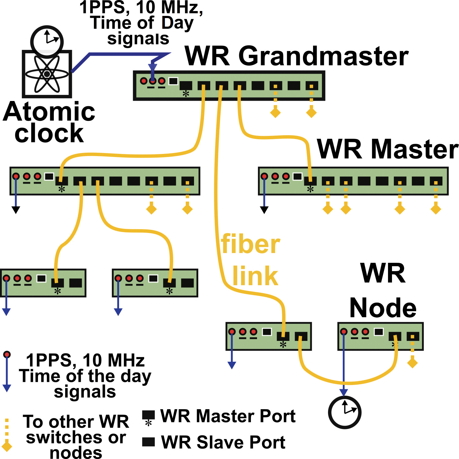
A central atomic clock provides synchronization references to a principal WR master switch dubbed the “grandmaster.” The grandmaster feeds synchronization signals into the network. which is expanded via fiber-connected WR devices: the switches and nodes of the network. These devices are serially linked to each other following a hierarchical master-slave pair configuration.

Accurate synchronization between a master and a slave WR-pair is performed as follows. The pair, which is connected via a bidirectional 1.25 gigabits per second optical Ethernet data link, quasi-continuously measures the round-trip delay of the data signals exchanged between the two devices. From these round-trip measurements, the one-way propagation delay, assumed symmetrical, is derived and compensated by the WR devices through an electronic control loop. To take into account possible asymmetries within a link, a calibration procedure is needed when initially installing the connection between a master and a slave. In practice, within smaller scale networks, the synchronization offset accuracy between devices is at the 100 picosecond-level. A 400-picosecond offset between WR devices has even been demonstrated over a distance of 169 kilometers, and more recently over a distance of 800 kilometers.

Besides the fiber-optic connection with other elements of the WR network, each switch or node can share its time-frequency references to an external device or system. These time-frequency references are available either in the form of IEEE 1588 Precision Time Protocol time stamps (via Ethernet connection), or in the form of electrical 1 pulse per second / 10 MHz synchronization signals (via coaxial cables).

THE CONCEPT

Centimeter- or even decimeter-level positioning accuracy is challenging to achieve using GNSS. In dense multipath environments, such as in urban canyons or indoor locations, the accuracy provided by GNSS is poor compared to the meter-level accuracy achievable in open terrain with the Standard Positioning Service. Moreover, GNSS services are vulnerable to interference, spoofing and jamming, and may be denied in indoor areas. We propose a TNPS based on a WR synchronization infrastructure as a complement to GNSS, providing higher timing and positioning accuracy, which also works in challenging environments.

TNPS can achieve decimeter-level accuracy in challenging environments through the use of wideband radio positioning signals. The attainable ranging precision is inversely proportional to the signal bandwidth. Furthermore, in dense multipath environments such as urban canyons, using wider bandwidth signals allows for finer time resolution. As a consequence, close-in received multipath components (MPCs) can be better resolved, and the LOS component can be more easily discriminated from delayed MPCs. This results in more accurate position solutions.

TNPS DEMONSTRATOR

We performed a demonstration of the concept in Delft, The Netherlands, at The Green Village (TGV), an experimental facility on the campus of the Delft University of Technology. The facility aims to accelerate development and implementation of innovations for a sustainable future (see FIGURE 2).

FIGURE 2. Implementation of the TNPS demonstrator. The time-frequency reference is provided by VSL and forwarded to TU Delft via optical fiber (in yellow) and distributed through the optical WR synchronization infrastructure. Wireless radio transmitters (green squares) connected to the WR network deliver wideband ranging signals to perform terrestrial positioning and navigation.

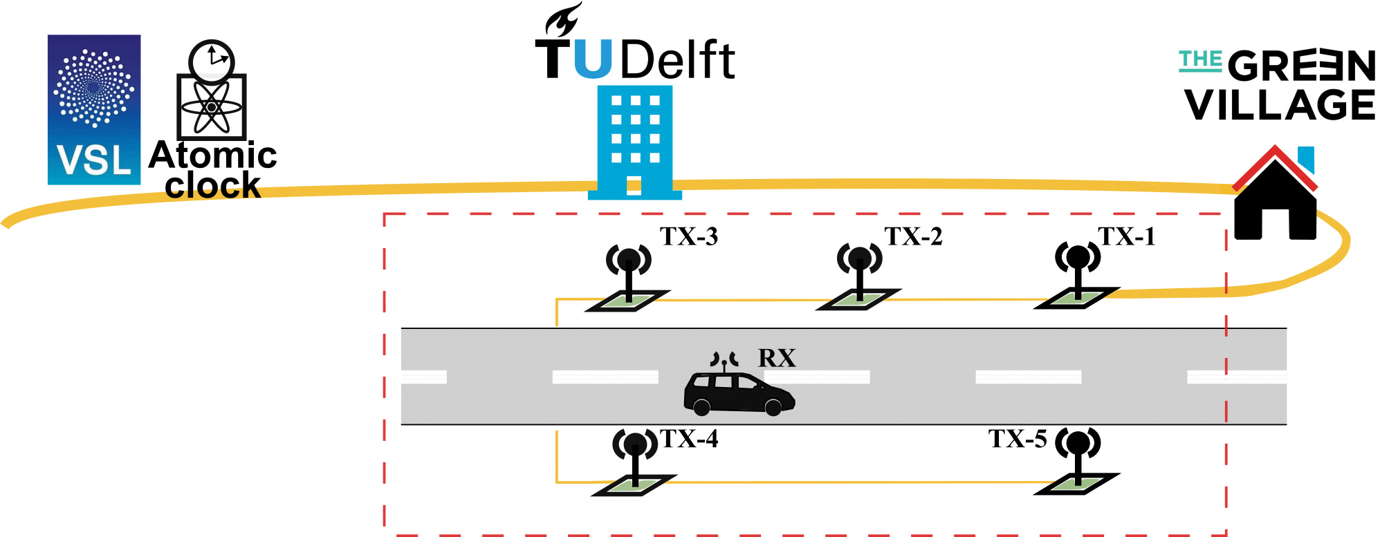
The central synchronization reference of the TNPS demonstrator is the Dutch national timescale version of Coordinated Universal Time UTC(VSL), derived from atomic clocks at the Van Swinden Laboratory (VSL), the Dutch metrology institute. The UTC(VSL) 10 MHz frequency reference and 1 pulse per second time reference are fed to the WR grandmaster switch (WR-SW1). The grandmaster switch is subsequently connected to a distant WR switch (WR-SW2) through a 1,470-nanometer downstream and a 1,490-nanometer upstream 1.25 gigabit per second optical link. WR-SW2, located at one of the TU Delft data centers, synchronizes in turn a WR node (WR-N1) installed at TGV.

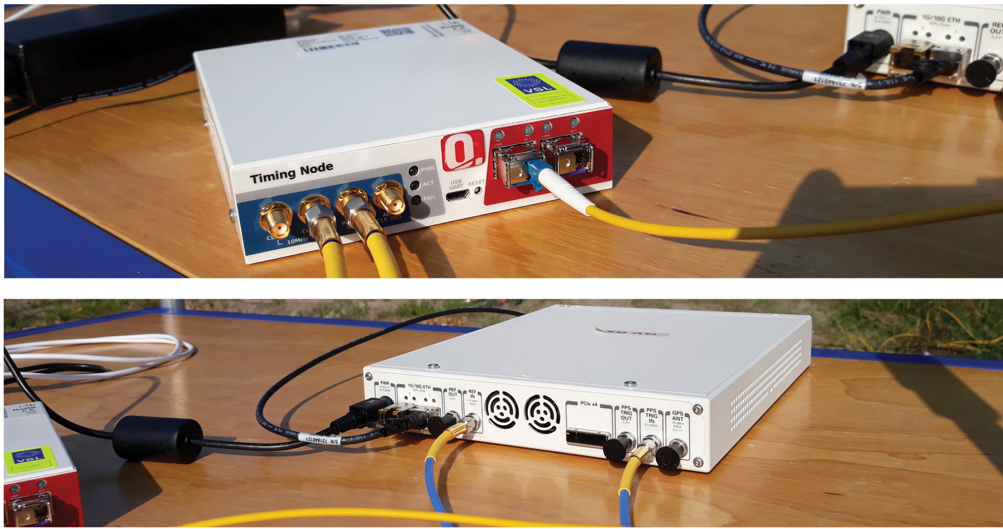
The remaining TNPS nodes at TGV are synchronized through a daisy-chain configuration. The first node (WR-N1) is connected to a second one (WR-N2), which is then connected to a third (WR-N3) and so on. In total, five timing nodes, WR-N1 to WR-N5, are connected to one another, using 50-meter optical fibers. These 5 timing nodes are used for synchronization (see FIGURE 3), and provide 1 pulse per second and 10 MHz electrical signals to five wideband radio transmitting units, uTX-1 to uTX-5, installed along a 50-meter stretch of road at TGV.

FIGURE 3. WR timing node (top) fed by a 1.25 gigabit per second bitstream through an optical fiber (yellow cable to the right) and providing electrical 1 pulse per second and 10 MHz synchronization signals at the outputs (two cables to the left). The bottom image shows an SDR system. The two channels of this device, capable of wideband operation, act here as a wireless transmitter or as a receiver. The transmitters are synchronized to the WR network through the 1 pulse per second and the 10 MHz electrical signals (blue-yellow cables at bottom) provided by the WR timing node.

A transmitting unit is based on a wideband transceiver: a software-defined radio (SDR) system linked to a wideband antenna that can operate from 700 MHz to 6 GHz. The antennas are connected to the SDRs using coaxial cables with a length of 5 meters and mounted on lampposts along the road at a height of about 4 meters. The transmitting units, uTX-1 to uTX-5, are respectively associated with antennas TX-1 to TX-5.

Each of these SDRs is capable of transmitting a wireless signal of up to 160 MHz bandwidth, on one or two of the device transmitter channels. The central frequency of each channel is tunable from 10 MHz to 6 GHz. In the demonstrator, we used a 3.96 GHz carrier frequency. The transmitting units periodically stream 160 MHz wideband quadrature phase-shift keying (QPSK) modulated pseudorandom noise (PRN) ranging signals sampled at 200 MHz. The five transmitters operate according to a time-division-multiplexing (TDM) scheme; uTX-1 to uTX-5 successively transmit the QPSK-modulated sequences as a 27.5-microsecond “burst” before turning idle. Between two successive transmissions, a guard interval of 3 microseconds is inserted during which all transmitting units are in idle state. It takes in total 150 microseconds for the five units to complete a transmission round, after which the units remain idle. The transmission round is then retriggered each millisecond.

At the receiver side (RX), another SDR platform is configured to acquire the QPSK modulated bursts transmitted by the five units uTX-1 to uTX-5. This SDR is actually playing the role of a data acquisition platform, which records and forwards the incoming sampled ranging sequences to the host PC via an Ethernet link. All processing and analysis in the demonstrator is performed offline, rather than in real time, using the collected ranging signals. The sampling rate of the acquisition platform is 200 MHz. A sample consists of a 16-bit in-phase value and a 16-bit quadrature-phase value (4 bytes in memory). In continuous operation, the SDR acquisition throughput would amount to 800 megabytes per second.

A throughput of 800 megabytes per second is difficult to handle for most of the host PCs. The SDR is therefore configured to only forward the relevant part of the data collected. Only the received samples time-aligned with the 150-microsecond transmitting window are periodically transferred to the host PC at a rate of 1 kHz. In practice, the acquisition window is slightly extended to 160 microseconds. Overall, the data throughput between the SDR and the host PC is now reduced to 128 megabytes per second; that is, 10 seconds of acquisition will generate a data file of 1.28 gigabytes.

A Schmidl & Cox synchronization sequence is embedded in the signal transmitted by uTX-1. The SDR field-programmable gate array continuously performs autocorrelation on the incoming samples and uses this sequence to detect the arrival time of the ranging bursts for operation in asynchronous mode. The receiver also can be operated in synchronous mode, that is, synchronized to a timing node.

TEST SETUP

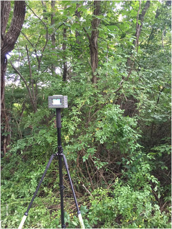
We carried out experiments on a 50-meter-long and 6-meter-wide local road at The Green Village (see FIGURE 4).

FIGURE 4. Test road at The Green Village, with three of the five roadside transmitting antennas (TX-3 to TX-5) as indicated. In the foreground, the receiver antenna is mounted on a trolley.

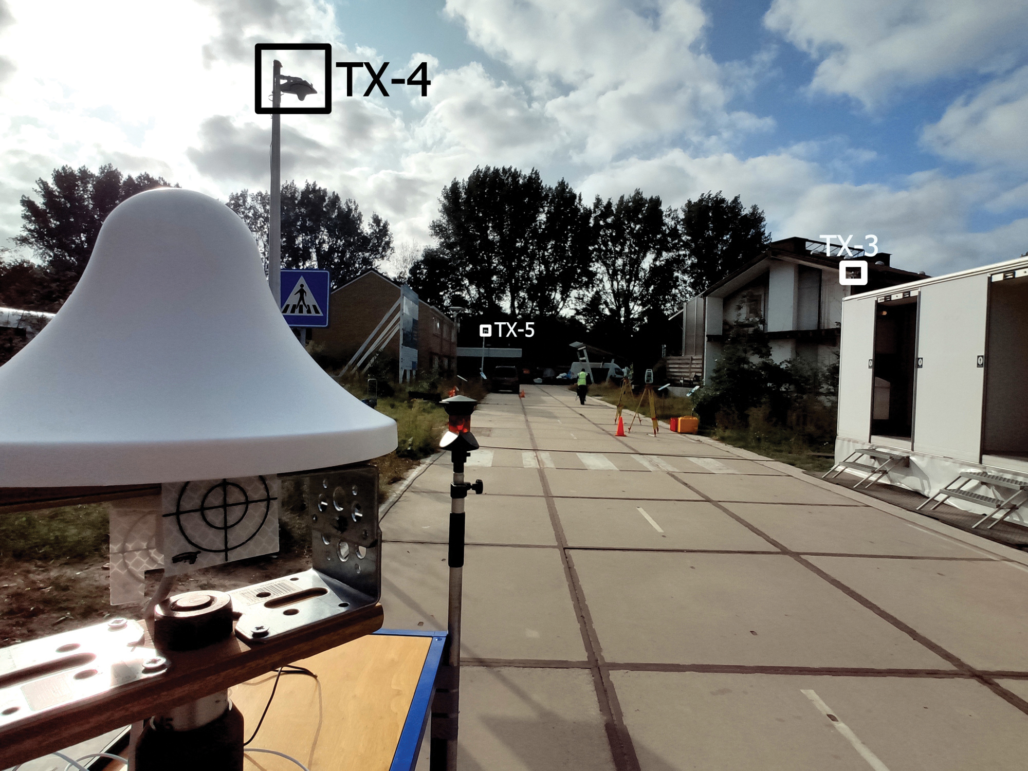
The road is bordered by built-up objects such as brick-wall houses, metal containers and large wooden advertising panels. These generate MPCs, which degrade the radio-positioning performance. The antennas TX-3, TX-4 and TX-5 can be seen mounted on lampposts. In Figure 4, the antennas TX-1 and TX-2 are on the right-hand sidewalk but not visible. The receiving antenna is in front to the left, mounted on a trolley. The RX antenna is identical to the ones used by the transmitters.

The receiver is used to perform a static survey at 50 locations on the road (staying at each point for around 1 minute). As shown in FIGURE 5, the receiver was also used for a kinematic experiment. The RX antenna is mounted on the roof of a car using a wooden beam. The RX antenna is linked via a 3-meter coaxial cable to the receiving SDR placed inside the car and connected to a host PC.

FIGURE 5. Receiver antenna mounted on the roof of a car. Two 360° prisms are used to determine the receiver ground-truth positions at the millimeter level, by means of land surveying total stations (placed on the yellow tripods in the distance).

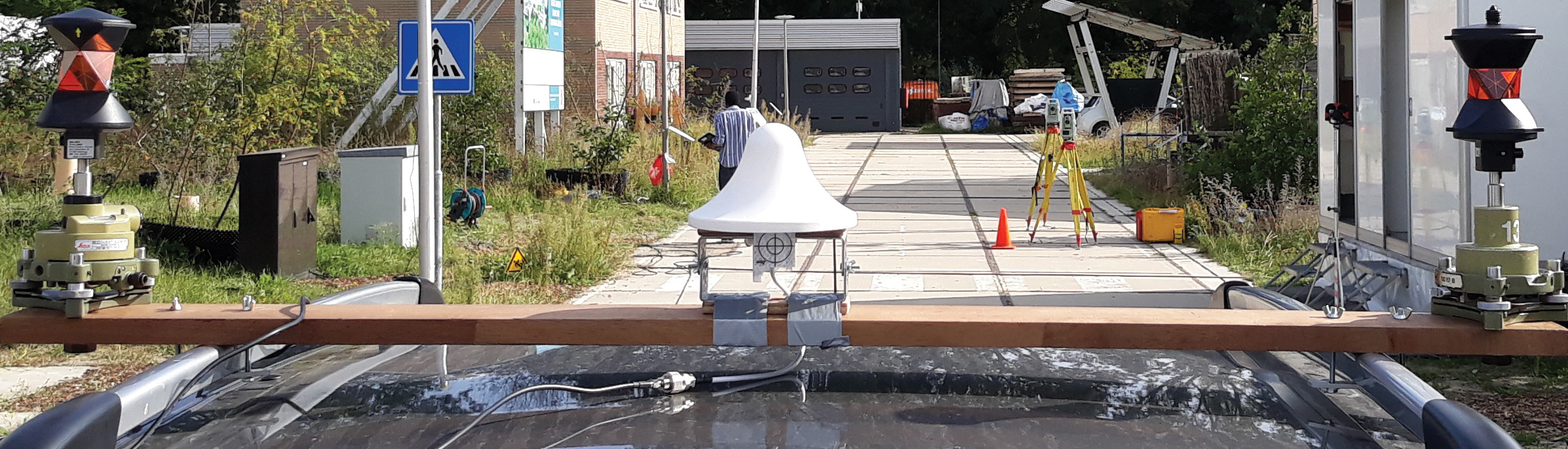
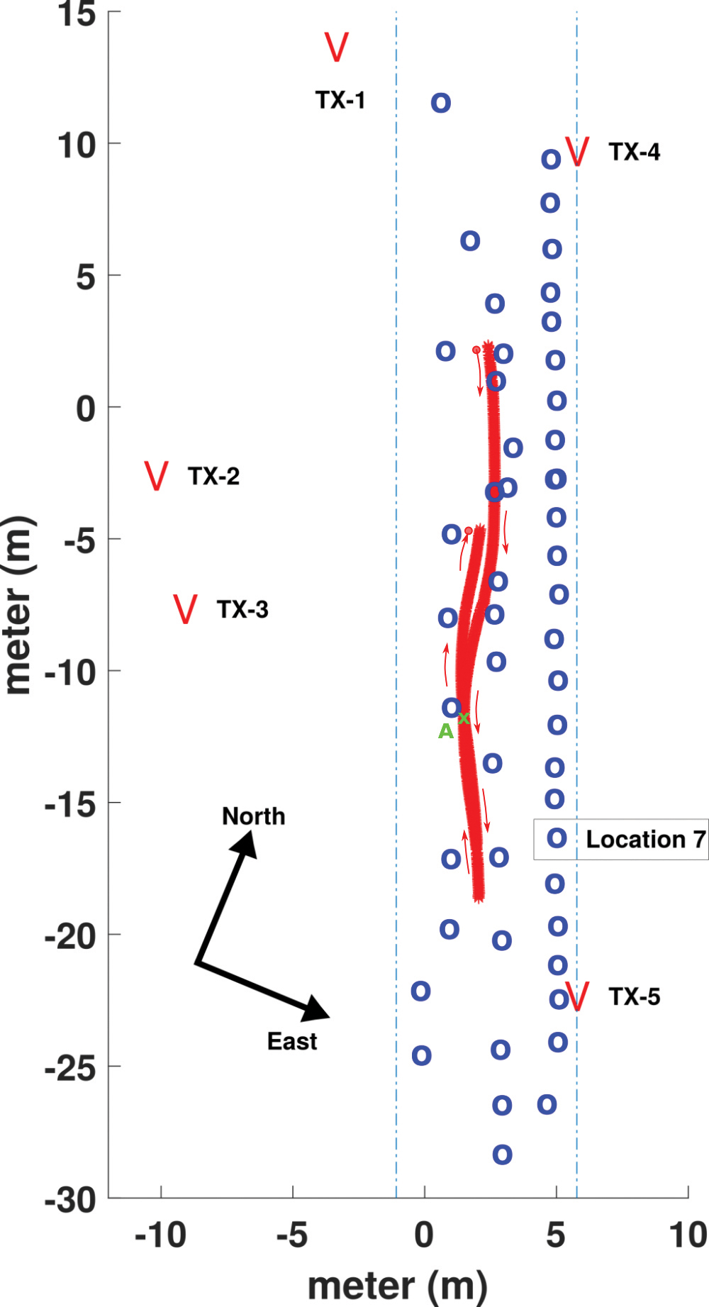
FIGURE 6 presents a map of the road with the static locations (in blue) and the forth-and-back kinematic track (in red). The transmitting antenna positions are indicated at both sides of the road.

FIGURE 6. Setup of the experiment on the local road at TGV. The locations of the transmit antennas, TX-1 to TX-5, are shown. Locations of static surveyed points are in blue, and the track of the kinematic experiment in red, with the RX antenna mounted on the roof of a car.

To establish a local coordinate system, the ground-truth positions of the RX antenna are determined using two land surveying total stations that rely on retro-reflective targets and 360° prisms to measure distances and angles. In Figure 4, a retro-reflective target, placed directly under the RX antenna, is visible, while the two total stations can be seen halfway down the road on the righthand side. In Figure 5, 360° prisms can be seen on both ends of the wooden beam on the roof of the car. The received signals are used to compute position solutions in post-processing, which are compared to the ground-truth values to assess the positioning accuracy. The accuracy of the ground-truth measurements is at the millimeter-level.

EXPERIMENTAL RESULTS

Achieving high positioning accuracy in a built-up area is difficult due to the presence of close-in MPCs, which arrive with very short time delays following the LOS component. FIGURE 7 shows the observed channel impulse responses (CIRs) between TX-1, TX-3, TX-5 and the receiver antenna RX placed at location 7 (see Figure 6). The LOS components can be easily detected as they correspond to the first and highest peak of each curve. However, we can also observe substantial close-in multipath components, which trail the main peaks. CIRs are obtained by division, in the frequency domain of the fast Fourier transform (FFT) of the received ranging sequences using the FFT of the known transmitted sequence. Oversampling by a factor of 100 is applied, as well as removing time delays of the TDM-scheme, such that the observed time delay difference directly represents the differences in ranges.

FIGURE 7. Normalized magnitude of the CIRs observed between the transmit antennas TX-1, TX-3 and TX-5 and the receiver antenna RX, positioned at reference point 7.

FIGURE 8. Time series of the positioning error in the east and north directions during the kinematic experiment.

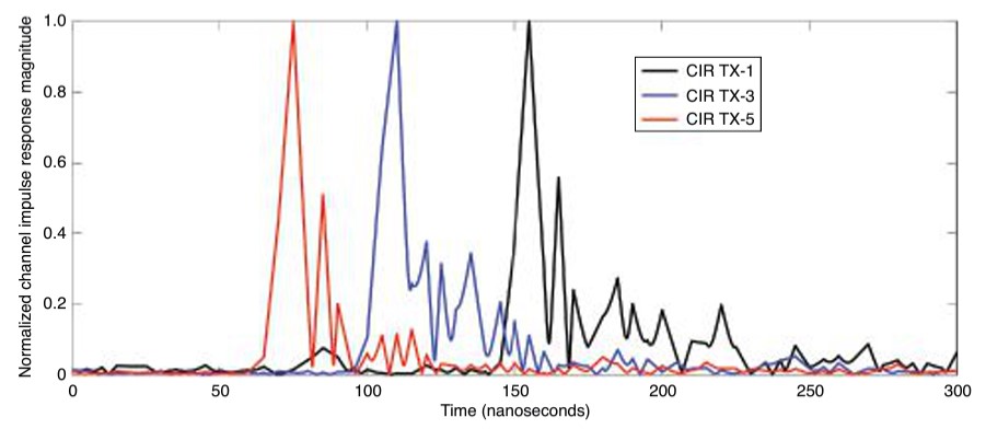
Since the TNPS signal bandwidth is 160 MHz, the time resolution is about 6.25 nanoseconds, which corresponds to about 1.9 meters of propagation distance. A multipath component, which arrives at the RX antenna with a lag larger than 6.25 nanoseconds with respect to the LOS component, is likely to be resolved and will not affect (bias) the ranging result. In this case, using time-of-flight techniques, ranges between TX and RX antennas can be determined, often at decimeter level, by extracting the time-of-arrival of the LOS components. Comparatively, if a 20 megasamples per second rate is used (corresponding to a 20 MHz bandwidth, commonly used in GNSS), the time resolution is 50 nanoseconds. An LOS component and a multipath component arriving at the RX antenna can likely be discriminated if the receiver and the reflector are separated by at least 15 meters. If the arrival time between the two components is less than 50 nanoseconds, then the MPC cannot be resolved and will cause a bias when determining the propagation distance between the TX and RX antenna.

The first and largest peak of each CIR seen in FIGURE 7 represents the LOS component. MPCs can be seen trailing the LOS, typically within the next 50 nanoseconds. The MPCs cause a bias in the estimated range when they cannot be resolved. Using wideband ranging signals allows for better time resolution, and better discrimination between the LOS component and the MPCs.

In the following, we assess the 2D positioning accuracy obtained using the demonstrator. 3D positioning is also possible with the demonstrator; however, since the TX antennas all are installed at similar heights and at a fairly low elevation compared to the RX antenna, we restrict our analysis to 2D positioning for the reason of having a poor geometry for determining the vertical position component. The 2D positioning model uses time difference of arrival (TDOA) pseudoranges allowing the cancellation of the asynchronous receiver clock offset. The frequency offset between the transmitters and the receiver has been estimated to be about 1 kHz, in asynchronous mode. After the TDOA ranges are computed from the experimental data, the 2D positioning problem is solved through Gauss-Newton iteration. Statistics of the static and kinematic 2D experiments are presented in TABLE 1.

TABLE 1. Static and kinematic positioning performance in terms of mean, standard deviation (std) and RMSE of position error, in east and north directions.

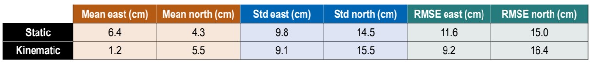
In the table, we present the mean position errors, standard deviations and root-mean-square errors (RMSEs) over the 50 surveyed points for the east and north directions. Mean errors of 6.4 and 4.3 centimeters are obtained for east and north directions, respectively. There is no significant bias in the system. In terms of RMSE, we can see that the positioning accuracy is just above 10 centimeters (11.6 and 15 centimeters respectively for the east and north directions). Overall, even with the presence of MPCs, and thanks to the synchronization accuracy and the wideband radio signals, a decimeter-level accuracy is achieved in static positioning.

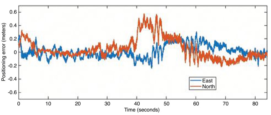
The duration of the kinematic experiment was 84 seconds. Looking at the statistics of the kinematic experiment, the results for the east and north directions show a small bias and RMSE values of 9.2 and 16.4 centimeters respectively. The positioning performance in static and kinematic mode is close, both for the east and north components. In both cases, positioning performance is better in the east direction than in the north direction. This may be explained by better spatial diversity of the antennas towards the east direction. The time series of the position errors for the kinematic experiment is presented in FIGURE 8. Overall, the track error in the eastern direction is within ±2 decimeters (at a 95% confidence level). For the northern direction, a larger deviation is observed in the observation time span from 40 to 50 seconds (forward track), where the error in the north direction is close to 4 decimeters. Such a deviation is likely due to close-in MPCs resulting in a degradation of the accuracy for that part of the track. As a consequence, 82% of the position error in this track lies within ±2 decimeters. Outside this time span, the performance in east and north directions is similar.

CONCLUSIONS

This article presents the concept and results of a demonstration of a TNPS that uses WR to synchronize the transmissions of wideband radio ranging signals to achieve decimeter-level position accuracy in multipath environments, such as in built-up areas. A proof of concept of the TNPS was implemented at TU Delft. The developed prototype system demonstrates a decimeter-level 2D positioning accuracy in an urban road-like configuration bordered by built-up surroundings that cause substantial multipath.

ACKNOWLEDGMENTS

The research described in this article is supported by the Dutch Research Council, Nederlandse Organisatie voor Wetenschappelijk Onderzoek. We thank Lolke Boonstra and Terence Theijn from TU-Delft ICT-FM, as well as Rob Smets of SURF, the collaborative organization for ICT for Dutch education and research for their support and expertise on the optical infrastructure, and Loek Colussi and Frank van Osselen of Agentschap Telecom and René Tamboer and Tim Jonathan of The Green Village for their support in realizing the SuperGPS demonstrator. We also thank project partners Koninklijke PTT Nederland (KPN), Optical Positioning Navigation and Timing (OPNT) and Fugro.

MANUFACTURERS

The WR timing nodes V1.15 are by OPNT. The SDR systems for the transmitters and receiver are National Instruments (Ettus) X310 Universal Software Radio Peripherals. The 3-dBi wide-band antennas CM.02.03 are from Taoglas.

CHERIF DIOUF was a postdoctoral researcher in the Department of Geoscience and Remote Sensing at Delft University of Technology (TU Delft).

HAN DUN was a Ph.D. student in the Department of Geoscience and Remote Sensing at TU Delft.

GERARD JANSSEN is an associate professor in the Circuits and Systems Group of the Microelectronics Department at TU Delft.

ERIK DIERIKX is the principal scientist at Electricity & Time at the national metrology institute VSL in Delft.

JEROEN KOELEMEIJ is an assistant professor in the Department of Physics and Astronomy at the Vrije Universiteit Amsterdam.

CHRISTIAN TIBERIUS is an associate professor in the Department of Geoscience and Remote Sensing at TU Delft.

May 14, 2022
Swift Navigation, SolarCleano: cleaning robots keep solar power running

A SolarCleano F1A robot tackles a tough cleaning challenge on a solar farm in Saudi Arabia. (Photo: SolarCleano)

SolarCleano, based in Garnich, Luxembourg, makes robots that clean large solar panel installations using GNSS receivers and corrections from Swift Navigation. We asked Christophe Timmermans, SolarCleano’s managing director, a few questions about its technology.

How often do solar panels need to be cleaned?

For decades, it was believed that solar panels did not need to be cleaned due to their angle to the ground and rain. Nowadays, however, the cleaning of solar panels is widely accepted as necessary to optimize a plant’s return on investment (ROI).

How much time per sq. meter do your machines take to clean solar panels?

To provide the fastest possible ROI to our customers, we developed a range of robots to best address the needs of various solar plant layouts. A large utility-scale project with high level of soiling losses in a desert environment will need a very fast and reactive cleaning solution such as our SolarBridge B1, which can clean 24/7/365 fully autonomously. The most suitable solution for a farm rooftop in Germany that needs to be cleaned three to four times a year might be our F1 model, which can clean the equivalent of up to two soccer fields a day. It is designed for rooftops, floating panels and mid-size plants up to 50 MW. While the speed of cleaning is a very important variable, the quality of cleaning is often considered as the driver to performance, which is why we propose different types of brushes depending on the soiling types. Plus, the robot speed can be modified according to the soiling level.

Why do robots need GNSS receivers to clean solar panels?

Moving on inclined, wet glass surfaces makes odometry unreliable because robots might occasionally slip. Therefore, GNSS is the most reliable way to continuously monitor their exact position. Our robots also need path planning because they cannot operate randomly like lawn mowers. Safety is obviously a major concern; we need a very high localization accuracy to ensure that robots don’t fall off the panels. Finally, the largest solar plants are developed in dry, remote locations with high irradiation such as the Sahara, Atacama and Australian deserts. GNSS allows us to have very accurate localization even in those remote areas. In addition, this solution can easily be installed on already-existing solar plants with little capital expenditure.

What spatial accuracy requirements do the robots have for this task?

Safety is our absolute priority. Therefore, our robots need an accuracy of less than 3 cm. They also need to be aware, in real time, of changes in their surroundings, such as maintenance teams, animals and uneven ground.

On large solar farms, GNSS receivers always have a clear line of sight to the satellites and do not suffer from multipath. So, what are the key technical challenges?

Our robots have the additional advantage that they do not need to drive very fast. However, we need to manage fleets of robots on the other side of the world in regions difficult to access and with harsh weather conditions, such as very high or low temperatures and the accumulation of dust behind panels due to air vortices. We need to be able to perform remote maintenance and solve any issue from our control center in Luxembourg. These challenges make our robots increasingly robust. With a current fleet of more than 300 robots around the world, we collect lessons every day to ensure a greater reliability for our upcoming generations of robots.

Why did you choose to partner with Swift Navigation?

We share a vision with Swift: “Accessible automated solutions serving sustainable goals.” We also share other important values, such as “iterate quickly” and “focus on what matters.”

March 31, 2022
ESA seeks ideas to augment satnav with imaging sensors, 3D maps

NAVISP includes projects for autonomous and connected driving. (Image: ESA/F. Bagiana)

The European Space Agency (ESA) is issuing a call for ideas to overcome GNSS service gaps in urban canyons by using imaging and 3D mapping technology. A workshop to discuss the call for ideas will be held virtually on July 6.

According to ESA, the growing availability of high-quality image sensors and high-fidelity 3D maps — such as those within smartphone mapping apps — offer a promising way to shrink the performance gap caused by urban canyons and multipath for future mobility applications in terms of ubiquity, reliability and resilience.

NAVISP — ESA’s Navigation Innovation and Support Programme — specifically is seeking prospects for technology demonstrations of mobility tech to support applications such as road, maritime transport and drones. The tech would provide assisted satnav by harnessing image sensors and 3D urban models. The proof-of-concept demonstration projects or national testbeds would facilitate introduction of this technology into commercial products.

Use cases include private or public autonomous transportation in cities, including cars, trams, scooters, bikes, urban ferries, harbors, narrow waterway navigation and future passenger drones.

Reflected satellite navigation signals (multipath) can degrade positioning performance, especially in urban canyons with numerous artificial surfaces. (Image: EUSPA)

The NAVISP project, called a “thematic window,” is titled “Assisted GNSS with Imaging Sensors and 3-D models for Mobility Applications.” The thematic window opened on June 10 and will close on Oct. 31. During its duration, ESA is offering dedicated support to companies interested in participating in the projects and submitting outline proposals.

On July 6, the agency is hosting an online workshop with stakeholders to raise awareness about the initiative and clarify any issues interested companies may have. ESA will present the requirements of the Thematic Window and the application process. The workshop will include presentations from high-level experts covering market perspectives, techniques involved in the use of 3D models and imaging sensors, the state of the art of these technologies and latest advances in visual navigation and artificial intelligence applied to mobility applications.

To register for the July 6 workshop, click here. The workshop agenda is available here.

June 21, 2021
Innovation: Monitoring sea level in the Arctic using GNSS
A Tidal Shift

Traditional tide gauges are in contact with the water surface and as a result are susceptible to measurement error and damage during extreme weather. An alternative approach is the use of GNSS reflectometry. We learn how this innovative use of satellite navigation signals works in this month’s Innovation column.

Innovation Insights with Richard Langley

Seawater level is conventionally monitored by tide gauges that measure the vertical distance of the water surface from a point on the ground. As the tide gauges provide seamless and highly accurate measurements, many countries operate a tide-gauge network to monitor sea-level changes and to assess flood risk. For example, the National Oceanic and Atmospheric Administration (NOAA) operates a permanent observing system, the National Water Level Observation Network (NWLON), with more than 400 gauges throughout the United States.

However, some challenges of tide gauges can be identified. Firstly, tide-gauge measurements require direct contact with the water, which causes limitations in installing and maintaining the equipment. The equipment requiring direct sensing is highly vulnerable to coastal hazards, such as coastal flooding and tsunamis, resulting in potential measurement errors or even equipment destruction during severe natural events.

Furthermore, tide gauges require maintenance on a regular basis, which is expensive because it requires the use of divers. This greatly limits the operation of tide gauges, especially in extreme environments such as in the Arctic. Alaska, for example, has significant gaps in its available spatially-varying tidal information. However, in the Arctic, it is also very important to constantly and closely monitor the long- and short-term variation of water levels because this area has a significant impact on global climate and ecosystems. Consequently, more support is needed for sea-level monitoring and coastal mapping in this region.

GNSS can serve as an alternative approach for water-level monitoring. GNSS satellites continuously transmit radio signals and ground-based, space-based, and airborne receivers access the signals regardless of weather conditions. Some of the received signals are reflected from obstacles or surfaces near the antenna, a phenomenon referred to as multipath (see FIGURE 1).

FIGURE 1. Schematic drawing of the GNSS-based tide gauge. (Image: Authors)

Multipath tends to be regarded as one of the major error sources for GNSS positioning where it causes unexpected phase delays when compared to the direct signal. Consequently, various procedures have been developed to mitigate the multipath effect. However, the GNSS signals reflected from the Earth’s surface contain information about the geophysical properties of the reflecting surface. The use of these signals is known as GNSS reflectometry (GNSS-R). GNSS-R allows us to monitor the temporal variation of water levels by calculating phase delays of GNSS signals reflected from the water surface. A GNSS-R-based tide gauge does not require direct contact with the water because it measures the water levels based on a remote-sensing technique. Thus, a GNSS-R-based tide gauge can be effectively applied to water-level monitoring.

However, several challenges exist in processing GNSS signals observed at high latitudes compared to mid-latitudes. Not only do we have to contend with extreme weather conditions and limited infrastructure availability, but also with problematic satellite geometry and ionospheric effects on the GNSS signals. To overcome these limitations in the use of GNSS-R in the Arctic, we introduce enhanced algorithms to improve the temporal and spatial resolutions of GNSS-R sea-level measurements.

Our approach includes an enhanced spectrum analysis based on multi-frequency signals and statistical reliability verification. Moreover, we include the signals transmitted by the Galileo constellation in addition to GPS to improve the quantity and the quality of GNSS observations in the Arctic. We have tested the proposed method with an experiment in Alaska and validated the results with nearby tide gauges. The experimental results clearly show the feasibility of employing GNSS-R-based tide gauges in the Arctic.

GNSS-R-BASED WATER-LEVEL MONITORING

Martin-Neria first introduced a method of monitoring sea level using the GNSS-R technique in 1993. Thereafter, many studies have been conducted to apply GNSS-R to water level estimation. Anderson proposed a method to estimate sea level using the interference pattern caused by the direct and reflected GNSS signals, which relies on the fact that the spacing between peaks in the interference pattern is almost entirely dependent on the height of the antenna above the reflecting surface.

The phase difference in the GNSS receiver between the direct and the reflected satellite signals varies while the geometry of a GNSS satellite changes (see Figure 1), generating the interference pattern. The interference pattern is particularly noticeable in signal-to-noise ratio (SNR) data. The reflected signals contribute to the SNR data in the form of oscillations, while the smoothly rising overall arc mostly depends on the signal strength and the antenna gain pattern.

The reflected signals can be isolated from the SNR data by removing the main trend — for example, by polynomial fitting — indicative of the direct signal. The frequency of the remaining dSNR oscillations is constant with respect to the sine of the elevation angle, assuming that the water level does not change during the satellite arc and the reflection surface is horizontal. Consequently, the frequency of the oscillation is linearly proportional to the height of the antenna above the reflecting surface.

The frequency can be derived from the dSNR data by spectral analysis. Among a number of spectral-analysis methods, the Lomb-Scargle periodogram (LSP) is commonly applied since it allows for processing of unevenly sampled data.

Determining the frequency of the oscillations. The antenna height above the water surface is directly calculated from the frequency of the oscillations derived from LSP processing. However, it is difficult to determine the dominant frequency because of the roughness of the water surface, especially in extreme environments such as Arctic regions with high currents and strong winds. In addition, the observed SNR data is easily affected by obstacles near the GNSS antenna. Therefore, it is difficult to distinguish the spectral peak of the signal reflected from the water surface from other additional reflected signals, especially when additional and unexpected reflections occur near the sea surface.

To minimize the erroneous determination of the frequency of the oscillations using dSNR, we can take advantage of the multiple frequencies of modern GNSS signals. In our study, we processed signals from both the GPS and Galileo constellations, with GPS transmitting three carrier signals (L1, L2 and L5) and Galileo transmitting five carrier signals (E1, E5a, E5b, E5ab and E6).

By comparing the spectrum peaks from the multiple signals on different frequencies, one can analyze the dominant peaks across the different frequencies on the same raypath. This algorithm is based on the fact that the multiple frequency signals should detect consistent sea-level heights because they are transmitted along the same raypath during the same period. One of the biggest advantages of this approach is that no additional data or equipment is required to accurately determine the frequency of oscillations of the GNSS signals reflected from the water surface.

Statistical Testing of Retrieved Sea Levels. Reflected signals are not necessarily all from the sea surface. To remove erroneous solutions, we conducted a statistical test. Data including measurement errors and/or some noise can be approximated to the model by the least squares method that determines the model parameters by minimizing the sum of squared residuals. However, this method yields an incorrect result when many outliers deviating from the normal distribution are included in the data set.

This problem can be overcome by applying RANdom SAmple Consensus (RANSAC). RANSAC stochastically estimates the model parameters maximizing consensus, that is, the parameter supported by the largest number of sample data through an iterative process. However, the RANSAC results can act differently each time for the same input data because it is essentially a statistical estimation method using random samples. Therefore, we perform RANSAC with rough constraints primarily to remove outliers significantly out of normal range, then the remaining noise in the data can be excluded by performing secondary fitting using tightly constrained least squares. For the least squares procedure, a series was applied for the fitting model, which represents various motions of the sea surface such as ocean tide loading, as a sum of trigonometric functions.

SEA-LEVEL MONITORING IN ST. MICHAEL

The Plate Boundary Observatory (PBO) network operated by UNAVCO (formerly the University NAVSTAR Consortium) is primarily designed to monitor long-term tectonic and volcanic deformation. However, it can also be used for GNSS-R applications. A new PBO station, AT01, was installed in May 26, 2018, in St. Michael, Alaska, which is designed to be suitable as a GNSS-R-based tide gauge with a clear and wide-open view toward the sea covering from 0° to 230° in azimuth (see FIGURE 2). The equipment at this site consists of a Trimble choke-ring geodetic antenna and a Septentrio PolaRx5 receiver that can receive not only GPS signals but also those of Galileo, with data recorded every 15 seconds.

FIGURE 2. The surrounding area of AT01 in St. Michael, Alaska: south view. (Photo: Authors)

We have used this station to assess our technique using one month of SNR data from June 2018. It should be emphasized that not only GPS but also Galileo signals were processed, and the Center for Orbit Determination in Europe’s Multi-GNSS Experiment final orbit and satellite clock products were used to minimize the satellite orbit error. Additionally, NOAA tide gauge stations (9468132 and 9468333) were used for comparison and verification of the water levels measured from the GNSS-R-based tide gauge (see FIGURE 3).

FIGURE 3. Locations of AT01 and two NOAA tide-gauge stations (9468132 in St. Michael and 9468333 in Unalakleet). The red box represents the zoomed area at the bottom right. (Image: Authors)

The 9468132 tide gauge in St. Michael is the nearest tide gauge at approximately 1.5 kilometers from AT01. However, since it is not operational, NOAA only provides water-level predictions (just high and low tides) based on the harmonic constituents, not the actual measurements. On the other hand, the 9468333 tide gauge in Unalakleet is approximately 74 kilometers away from AT01. This makes it difficult to use the tide gauge as ground truth, but it does provide the actual sea-level measurements including any abnormal daily variations during the observation period. Therefore, we used the water-level predictions and measurements from both stations to validate the GNSS-R-based water-level measurements at AT01.

Determination of Water Level. The GPS and Galileo SNR data were independently analyzed using our in-house software package (written in MATLAB) using the following procedures.

As a preprocessing step, each SNR data series was examined to filter out the signals reflected from other surfaces surrounding the antenna and to isolate the signals that were reflected by the sea surface. Since AT01 PBO station was installed to investigate the feasibility of its use as a GNSS-R-based tide gauge, the most effective azimuth and elevation ranges were given, which are 0° to 230° and 10° to 25°, respectively.

The azimuth and elevation angle ranges were applied, which effectively removed reflected signals from surfaces other than the sea surface. After identifying the SNR data affected by the reflection from the sea surface, the processing windows were dynamically determined by the continuous path and direction (ascending and descending) of the satellites, and the height of the sea surface was estimated using only a portion of the satellite arc contained within each processing window.

For example, FIGURE 4 shows the processing windows determined for the GPS satellite PRN 1 on June 1, 2018. The red dots in the figure show the parts of the satellite arcs affected by multipath from the sea surface. The data was divided into three processing windows due to the arc discontinuities and satellite path directions. It should be noted that only the processing windows with a data span of 30 minutes or longer were used for water level estimation. This minimum data span duration of 30 minutes was empirically determined by observing the probability of failure of the water -level calculation for shorter spans.

FIGURE 4. An example of the processing window determination for GPS satellite PRN 1 on June 1, 2018. (Image: Authors)

To isolate multipath effects from the SNR observation, we removed the trend in the SNR by a second-order polynomial fitting using only the portion of a satellite arc contained within each window. FIGURE 5 (b) shows the detrended SNR (dSNR) from FIGURE 5 (a), and the impact of the multipath is clearly identified in the form of the oscillation. As discussed earlier, the oscillation frequency is related to the antenna height above the sea surface. Accordingly, the dSNR data was analyzed through an LSP. As shown in FIGURE 5 (c), multiple peaks are founded from the LSP results of each dSNR series, and it is not easy to distinguish the frequency of the reflected signal from the sea level among these peaks.

Since multiple frequency signals from the same satellite must detect the same sea-level height, the final dominant peak was determined by checking the consistency of the resulting heights from each dominant peak among the multi-frequency signals. After that, the dominant frequency was converted to the antenna height above the reflection surface, which was then subtracted from the orthometric height of the antenna (the height above the geoid or, approximately, the height above mean sea level [MSL]) to refer the height of the instantaneous sea surface to MSL.

FIGURE 5. SNR data-analysis procedures with PRN 1 GPS on June 1, 2018: (a) The SNR data affected by the reflection from the sea surface, (b) detrended SNR data through a second-order polynomial, and (c) LSP results and dominant peaks of each frequency. (Image: Authors)

After analyzing all SNR data observed during one day, we carried out the reliability test of the retrieved sea levels to reject erroneous sea-level solutions.

RESULTS AND VALIDATION

The water-level changes from the GNSS-R-based tide gauge at St. Michael were compared to the independently predicted and measured sea levels from the neighboring St. Michael and Unalakleet tide gauges during June 1–30, 2018. Although the tide gauges are considered reliable ground truth, our experimental study must take into account the physical distance between the sites (about 1.5 and 74 kilometers from AT01, respectively) as well as the difference coming from the model versus the actual measurement.

In addition, a vertical offset between the data time series of the GNSS-R-based tide gauge and the standard tide gauges should be considered due to their different datums. Whereas the GNSS-R-derived sea level refers to a geodetic datum — namely the U.S. National Spatial Reference System (NAVD 88) — a standard tide gauge is highly localized with reference to a tidal datum such as local mean sea level. Generally, the difference between the geodetic and tidal datums is provided by NOAA, which allows us to convert between two vertical datums.

However, the vertical datum in Alaska has significant gaps in the spatially varying tidal information because of the difficulties of operating tide gauges there so that accurate information for datum conversion cannot be obtained. Therefore, the averages of the vertical differences were calculated (–6.44 centimeters for the St. Michael tide gauge and 9.54 centimeters for the Unalakleet tide gauge), which were then applied to each of the time series to make the comparisons. In fact, such a problem implies another advantage of a GNSS-R-derived tide gauge: it already returns a water-level height based on the terrestrial datum so that the datum of the land and the ocean can be consistently retained.

FIGURE 6 shows the sea level derived from the GNSS-based tide gauge measurements using GPS (red dots), Galileo (blue dots), the predicted sea level from the St. Michael tide gauge (green dots and lines) and measured sea level from the Unalakleet tide gauge (blue line).

FIGURE 6. Time series of sea level derived by GNSS-R-based tide gauge (AT01) in St. Michael, Alaska, during a month (red and blue dots for GPS and Galileo satellites, respectively; yellow dashed lines for the smoothed time series from two hours’ moving average filter) together with sea-level measurements from the Unalakleet tide gauge (blue solid line) and sea-level predictions from the St. Michael tide gauge (green dots for high- and low-tide predictions and green dashed line for interpolated predictions). (image: Authors)

The overall results show good agreement with the tide predictions at the nearby St. Michael tide-gauge station. It should be noted that the St. Michael tide gauge only provides high- and low-tide predictions so these were interpolated. However, some tidal characteristics not represented in the published predictions were also confirmed. In particular, as shown in the red-shaded segments of the time series marked (a) and (b) in Figure 6, larger and lower amplitudes than the tide predictions for the St. Michael tide gauge were identified on June 3 and 16, respectively.

These inconsistencies can be explained by the comparison with actual sea-level measurements at the Unalakleet tide gauge (solid blue line in Figure 6), which show very similar sea-level changes compared to those of the GNSS-R-based tide gauge. In addition, the overall larger amplitudes in the time series from the Unalakleet tide gauge can be explained by considering the fact that the amplitudes of the water levels vary along the coastline in Alaska and the Unalakleet tide gauge is approximately 74 kilometers from AT01.

To quantitatively investigate the agreement between the GNSS-R-based tide gauge and the standard tide gauges, we computed correlation coefficients. To ensure simultaneous data, the standard tide-gauge measurements and predictions were interpolated to the time tags of the GNSS-R-based time series. The correlation coefficients are 0.87 and 0.81 with the St. Michael and Unalakleet tide gauges, respectively.

The statistical analysis of the comparison result is summarized in TABLE 1. The mean and maximum values were computed using the absolute sea-level differences. From the results, it could be established that the GNSS-R-derived sea level shows better agreement with actual sea-level measurements at the Unalakleet tide gauge even though it is approximately 74 kilometers away from AT01.

Table 1 Statistical analysis of the sea-level differences between the GNSS-R-based tide gauge (AT01) and the standard tide gauges (Unalakleet and St. Michael).

Spectral analysis was additionally conducted to validate the sea levels from the GNSS-R-based tide gauge. Because the St. Michael tide gauge does not provide actual measurements (only predictions), only the Unalakleet tide gauge was used in the spectral comparison. A fast Fourier transform (FFT) was applied to convert the time series of the sea levels to the frequency domain.

The GNSS-R-based tide gauge showed good agreement with the Unalakleet tide gauge overall. In addition, from the corresponding spectral analysis results, we were able to find meaningful harmonic constituents, M2, K1 and O1. The harmonic constituents estimated from the sea-surface measurements of the GNSS-R-based tide gauge have amplitudes most similar to the published harmonic constituents of the nearest St. Michael tide gauge, although the difference in amplitudes of the three harmonic constituents averages 12.3 centimeters.

In fact, the Unalakleet tide gauge also does not exactly match the amplitude of the estimated harmonic constituents and the published harmonic constituents. But by summarizing the corresponding results, we can conclude that the harmonic constituents estimated from the GNSS-R-based tide gauge are reliable.

As mentioned earlier, in our study, we estimated the water-level change by using GPS and Galileo satellite signals to overcome the degradation of GNSS performance due to the satellite geometry in the Arctic. The smoothed time series, calculated from a moving-average filter of two-hour intervals, is shown in Figure 6 (yellow dashed lines). The time series of sea level derived by the GNSS-R-based tide gauge during the whole month were used as ground truth for evaluating the accuracy.

This was done because the Unalakleet tide gauge is approximately 74 kilometers away from AT01 and the St. Michael tide gauge does not provide actual measurements, making it difficult to use as ground truth. As a result, the sea levels determined using the Galileo and GPS signals showed very similar accuracy with an average difference of 0.11 meters. Therefore, even if Galileo is additionally used, the estimated final water levels were at a similar level of accuracy.

However, the number of water-level observations dramatically increased (approximately doubled) when GPS and Galileo signals were both involved, even though the number of Galileo satellites is fewer than the number of GPS satellites. This is because Galileo transmits on five frequencies while GPS transmits on just three, so we can achieve more robust solutions by including Galileo.

We investigated how adding Galileo satellites changes the temporal resolution of the final sea-level measurements. At this time, several sea-level measurements pointing to the same epoch (such as sea levels from several frequency observations of the same satellite arc) were considered as one measurement for the time interval computation.

Overall, sea-level measurements using only Galileo satellites show lower temporal resolution compared to GPS satellites alone, with a mean time interval of 48.97 minutes because Galileo is not fully operational yet and fewer satellites are available. However, combining GPS and Galileo satellites to the sea-level analysis significantly increased the time resolution.

When only GPS satellites were used, the maximum time interval between two water-level measurements was greater than 3 hours, while the maximum time interval was shortened to about 1.5 hours when Galileo satellites were included in the water-level measurement.

However, even if both GPS and Galileo satellites were used, the average time interval was still 14.1 minutes, which is considerably longer than the time resolution of the standard tide gauge of 6 minutes. The lower time resolution of a GNSS-R-based tide gauge is explained by the limited ranges (azimuth and elevation angle ranges of 0° to 230° and 10° to 25°, respectively) toward the ocean at station AT01. It means the time resolution can be improved by securing a wider view of the ocean from the GNSS-R-based tide gauge.

SUMMARY AND CONCLUSION

The purpose of our study was to evaluate and verify the feasibility of using GNSS-R for sea-level monitoring in the Arctic. We used data from a GNSS station in St. Michael, Alaska, and applied an advanced algorithm that accurately determines sea levels through the comparisons of results from multiple GNSS signals along with an effective filtering procedure. Our results were validated through comparisons with measurements and predictions from nearby standard tide gauges.

From the corresponding analysis, we could confirm that the GNSS-R technique overcomes the limitations of standard tide gauges in the Arctic and successfully estimated the sea-level change in St. Michael, Alaska. The results from this study show many promising applications for a GNSS-R-based tide gauge in the Arctic, such as tsunami and flood monitoring and tidal datum determination.

In future studies, additional research should be conducted on how well the GNSS-R-based tide gauge can operate in extreme conditions such as low temperatures, wind gusts, storms, and snow. And, for further improvement of the temporal resolution of the technique, all active GNSS constellations including GPS, GLONASS, Galileo, and BeiDou should be included — that will certainly improve the temporal resolution and also potentially improve the accuracy and reliability. It would be also worth studying the spatial variations of sea-level changes by investigating the specular reflection points of GNSS multipath signals.

ACKNOWLEDGMENTS

This article is based on the paper “Monitoring Sea Level Change in the Arctic Using GNSS-Reflectometry” presented at ION ITM 2019, the 2019 International Technical Meeting of The Institute of Navigation, Reston, Virginia, Jan. 28–31, 2019.

SU-KYUNG KIM is a graduate research assistant at Oregon State University in Corvallis, Oregon. She received her M.Sc. in geoinformation engineering from Sejong University in Seoul, South Korea, in 2013. Her research interests are focused on sea-level change monitoring and crustal deformation studies using GNSS.

JIHYE PARK is an assistant professor of geomatics at Oregon State University. She holds a Ph.D. in geodetic science and surveying from The Ohio State University in Columbus, Ohio. Her research interests include GNSS positioning and navigation, GNSS reflectometry, ionospheric and tropospheric monitoring for natural hazards and artificial events, and other geospatial-related topics.

FURTHER READING
- Authors’ Conference Paper
“Monitoring Sea Level Change in the Arctic Using GNSS-Reflectometry” by S.-K. Kim and J. Park in Proceedings of ION ITM 2019, the 2019 International Technical Meeting of The Institute of Navigation, Reston, Virginia, Jan. 28–31, 2019.
- Pioneering Work by Manuel Martin-Neira
“The PARIS Concept: An Experimental Demonstration of Sea Surface Altimetry Using GPS Reflected Signals” by M. Martín-Neira, M. Caparrini, J. Font-Rossello, S. Lannelongue and C.S. Vallmitjana in IEEE Transactions on Geoscience and Remote Sensing, Vol. 39, No. 1, 2001, pp. 142–150, doi: 10.1109/36.898676.

“A Passive Reflectometry and Interferometry System (PARIS): Application to Ocean Altimetry” by M. Martín-Neira in ESA Journal, Vol. 17, No. 4, 1993, pp. 331–355.
- Using GNSS Reflectometry to Monitor Water Level
Local Sea Level Observations Using Reflected GNSS Signals by J.S. Löfgren, Ph.D. dissertation, Chalmers University of Technology, 2014.

“Coastal Sea Level Measurements Using a Single Geodetic GPS Receiver” by K.M. Larson, J.S. Löfgren and R. Haas in Advances in Space Research, Vol. 51, No. 8, 2013, pp. 1301–1310, doi: 10.1016/j.asr.2012.04.017.

“Monitoring Coastal Sea Level Using Reflected GNSS Signals” by J.S. Löfgren, R. Haas and J.M. Johansson in Advances in Space Research, Vol. 47, No. 2, 2011, pp. 213–220, doi: 10.1016/j.asr.2010.08.015.

“Three Months of Local Sea Level Derived from Reflected GNSS Signals” by J.S. Löfgren, R. Haas, H.-G. Scherneck and M.S. Bos in Radio Science, Vol. 46, No. 6, 2011, RS0C05, doi:10.1029/2011RS004693.

“Determination of Water Level and Tides Using Interferometric Observations of GPS Signals” by K.D. Anderson in Journal of Atmospheric and Oceanic Technology, Vol. 17, No. 8, 2000, pp. 1118-1127, doi: 10.1175/1520-0426(2000)017<1118:DOWLAT>2.0.CO;2.
- Earlier Innovation Columns Dealing with GNSS Refectometry
“How Deep Is That White Stuff? Using GPS Multipath for Snow-Depth Estimation” by F.G. Nievinski and K.M. Larson in GPS World, Vol. 25, No. 9, September 2014, pp 38–50.

“Friendly Reflections: Monitoring Water Level with GNSS” by A. Egido and M. Caparrini in GPS World, Vol. 21, No. 9, September 2010, pp 50–56.

“It’s Not All Bad: Understanding and Using GNSS Multipath” by A. Bilich and K.M. Larson in GPS World, Vol. 20, No. 10, October 2009, pp. 50–56.
- Tides and Water Level
Tides, Surges and Mean Sea-Level by D. Pugh, published originally by J. Wiley & Sons, Chichester, U.K., 1987, reprinted with corrections in 1996 and subsequently issued in e-print form by NERC Open Research Archive.
- Random Sample Consensus
“Random Sample Consensus: A Paradigm for Model Fitting with Applications to Image Analysis and Automated Cartography” by M.A. Fischler and R.C. Bolles in Communications of the ACM, Vol. 24, No. 6, 1981, pp. 381–395, 10.1145/358669.358692.
- Vertical Datums
“Vertical Datum Transformation: Integrating America’s Elevation Data.”
- NOAA Tides and Currents
Local water levels, tide and current predictions, and other oceanographic and meteorological conditions are available on this NOAA website.
October 21, 2019
Spirent Sim3D provides realistic multipath simulation

3D modeling solution creates true-to-life synthetic environments for more accurate testing.

Spirent Communications plc has launched an innovative multipath simulation solution, Spirent Sim3D. The 3D modeling solution enables the testing of realistic multipath and obscuration effects on GNSS signals in a true-to-life synthetic environment.

Sim3D is suitable for use by automotive, chipset, handset and receiver manufacturers, as well as in aerospace, military, mining and precision agricultural applications.

Spirent will demonstrate Sim3D at ION GNSS+ 2019 in Miami, Florida, Sept. 16-20.

Studying multipath. Historically, researchers and developers of GNSS receivers have had to rely on statistical models and time-consuming field testing to study the effects of multipath on GNSS signals.

With Sim3D, the industry can now gain a greater understanding of the impact of multipath and obscuration in a broad range of real-life situations. It offers the level of control and traceability needed for developers to improve their customers’ experience in the most challenging environments.

A satellite signal reflecting off surfaces, such as a building, a high-sided vehicle, a tree, or even the ground, alters the pseudorange, causing the signal to arrive at the receiver slightly later than line-of-sight signals.

Without proper mitigation, this can cause a receiver to output an inaccurate position.

“Obscuration and multipath effects are one of the major obstacles faced by engineers trying to achieve accurate GNSS positioning solutions,” said Spirent Managing Director of Positioning Martin Foulger. “The accelerating development of connected autonomous vehicles and other precision applications means the need to test for higher precision positioning, navigation and timing in a variety of environments is growing rapidly. Sim3D is an important and timely development.”

Image: Spirent

Simulation of 3D environments. The unique system has been developed in partnership with OKTAL Synthetic Environment. It offers the ability to simulate multipath effects in a range of lifelike geo-typical environments, using different models to recreate locations such as urban highway, an inner city or a forest. Geo-specific models of real locations can also be commissioned.

During simulation with Sim3D, the GNSS signals interact with fully customizable 3D environments to simulate real-life applications in operation, like a vehicle on a highway, or a wearable device on a pedestrian.

This gives a level of detail, control and realism in testing not previously available. Such realistic multipath and obscuration simulation will add greater credibility to GNSS testing and assure that developed solutions are optimized and tested for their intended environments.

“As vehicles become increasingly autonomous, it’s vital to get a more detailed understanding of the effects of obscuration and multipath on a vehicle’s ability to generate an accurate GNSS-based position” explained Foulger. “Statistical models cannot sufficiently achieve this.

“Sim3D’s ability to realistically simulate different environments provides this greater accuracy and brings a host of benefits to researchers and developers of autonomous vehicle systems,” Foulger said. “It will help to guide critical design decisions like where to place the GNSS antenna on the vehicle, what GNSS receiver to use and when to hand over to other position sensors as GNSS signals degrade.”

August 29, 2019
New GPS receiver uses multipath for better time synchronization

A new receiver for GPS and other GNSS improves time-synchronization accuracy in areas with severe reception conditions, such as among buildings and in mountainous areas.

The receiver was developed by Nippon Telegraph and Telephone Corporation (NTT) and Furuno Electric Co. Ltd.

Furuno plans to begin sales of the new GF-88 series time synchronization GNSS receivers in April 2019, and to deploy it widely in fields such as 4G/5G mobile base stations, financial trading, power grids and data centers.

The GF-88’s new algorithm makes use of multipath signals, those reflected or diffracted from buildings and other structures, which previously inhibited accuracy of time synchronization.

By integrating a new satellite signal selection algorithm developed by NTT into Furuno’s time synchronization GNSS receiver, in addition to signals from satellites in line-of-sight locations, multipath signals can be used to reduce time error, the companies said.

In a real multipath reception test environment, time error was reduced to approximately one fifth of earlier values.

The remarkable result promises to enable time synchronization accuracy close to that obtained in open-sky reception environments with no obstructions, even in environments previously considered poor and unsuitable for accurate time synchronization, such as among buildings or in mountainous areas.

The companies will exhibit the results at Tsukuba Forum 2018 Oct. 25-26, and at ITSF 2018, in Bucharest, Romania, Nov. 5-8.

More information is available here.

Satellite selection algorithm. (Image: NTT/Furuno)

GNSS receiver prototype performance test results, (Image: NTT/Furuno)

November 1, 2018
Simulating multipath in real time for receiver evaluation
By Tommaso Panicciari, Mohamed Ali Soliman and Grégory Moura
All images provided by the authors

A real-time system combining a simulator and a GNSS propagation model reproduces an authentic multipath environment. The propagation model relies on a 3D-model reconstruction of the urban environment, which generates a multipath signature strictly dependent on the location of the receiver’s antenna. This yields important results for a moving vehicle, which may be affected by very different multipath conditions depending on trajectory and location.

Positioning and navigation can be degraded in urban environments by multipath, and the error can increase considerably if not properly compensated. In situations where the line-of-sight (LOS) is obscured by surrounded buildings, the receiver may still be able to navigate by using the non-line-of-sight (NLOS) signal, which originates from single or multiple reflections/diffractions of the GNSS signal.

The use of 3D models has been one of the preferred solutions to recreate the multipath environment as seen by a GNSS device. This solution brings the capability to generate a multipath signature that is representative of the position of the antenna in a specific time and space. However, this solution comes with a certain degree of complexity. In fact, an accurate 3D model is required to simulate the obscuration of the GNSS signal, and a good propagation model is needed to generate phenomena like reflection and diffraction.

Figure 1. Example of propagated signal simulation. (Image: Tommaso Panicciari, Mohamed Ali Soliman and Grégory Moura))\

3D models have become more accurate and widely available and are mainly used to predict the satellite availability in specific locations, for example in evaluating the signal availability in urban canyon, and for both reflection and diffraction. Other uses of 3D models are as an aiding tool to assist navigation, sometimes together with an INS solution.

In this article, we present a novel real-time system capable of simulating realistic multipath in different environments. The system can simulate multiple GNSS constellations and is comprised of a GNSS simulator interfaced to a propagation model. The system can create a whole range of signals, effects, error models and trajectories in a real-time closed loop. The propagation model controls the simulation of multipath from the interaction of the GNSS signal with the 3D scene and objects. This article describes a novel real-time system for the simulation of realistic multipath in different environments and compares simulated and field-test data. The comparison is based on signal availability, horizontal error, carrier-to-noise (C/N₀), pseudorange and Doppler residuals.

RAY-TRACING WITH 3D MODELING

The model simulates the propagation of GNSS signals in constrained environments, considering obscurations and multipath. It uses a proprietary ray-tracing kernel (based on bounding volume hierarchy techniques using processing unit [GPU] resources) coupled with geometrical optics and uniform theory of diffraction to compute the interaction between the signal and the local environment. The computation uses as main input a synthetic environment (that is, geometrical and physical modeling of a real or realistic environment) to assess the impact of obscurations related to signal availability issues and multipath (the cause of fading effects and performance problems).

The objective of ray-tracing is to find all the possible paths from the observer to the source of the signal considering a limited number of interactions per emitted rays. A ray-tracer (or ray-tracing algorithm) uses a primary grid to cast primary rays. Then, it iteratively computes the possible interactions between these rays and the virtual scene (often defined using triangles). If those interactions exist (if they comply with the law of physics) and if the number of interactions to reach the emitter is below the maximum number of interactions set by the user, then a ray (or multipath) is created. This is a deterministic method that can be used to calculate the obscuration due to the local environment (and therefore detect the signal availability) and the geometrical characteristic of the computed path. Combined with physics modeling, path attributes such as received power, delay, Doppler, and phase are also provided.

The main characteristics of ray-tracing techniques to model GNSS propagation are:
- All the signals arriving at the receiver can be model-based on the virtual environment.
- As it is a deterministic method, the more realistic the environment modeling, the more compliant with reality the results. Moreover, the simulation results are repeatable.
- The specular multipath can be displayed in 3D, and the attributes (for example, receiver power, phase, polarization, Doppler, geometry of the ray) are known. For example, this is relevant when the effect and signature of the environment on the propagation signal need to be studied and understood.
Nonetheless, ray-tracing techniques must account for three major difficulties:

They are time-consuming algorithms. Indeed, depending on the complexity of the scene (defined in terms of the number of triangles), a combinatorial problem to find the possible multipaths reaching the receiver makes the ray-tracer very resource-demanding. That is the reason why the most difficult task to achieve during the coding of a real-time ray-tracing algorithm is to develop acceleration techniques to quicken the computation process. Several solutions exist to either improve the intersection determination (for instance, based on spatial hierarchies such as bounding volume hierarchy [BVH] techniques), or to decrease the number of cast rays (often based on adaptive sampling techniques), or even to replace rays with beams or cones. Moreover, it is possible today to use the resources of graphic boards to accelerate the computation. Indeed, as ray-tracing can be coded by a large number of primary functions that can be treated simultaneously, it can be easily ported into GPU.

Their accuracy depends on the resolution of the primary grid. Details and therefore rays may be missed if the 3D scene is made of small details. This issue is called aliasing. Aliasing artefacts are raised for instance in parts of the scene with abrupt changes (such as edges) or in complex areas with lots of constituent objects. Solutions (or antialiasing techniques) exist to overcome this issue such as adaptive or stochastic samplings.

When it is combined with geometrical optics, these algorithms only compute the specular rays. Even if some techniques exist to model the scattering signals, only physical optics can render the global signal with high fidelity.

MULTIPATH SIMULATION SYSTEM

The proposed system can model two of the main propagation issues encountered in urban environments, such as obscuration (which leads to limitations in signal availability) and multipath (which generates interference that causes fading of the signal and positioning errors). To model realistically such a complex phenomenon, the system uses a GPU ray-tracing algorithm combined with geometrical optics and uniform theory of diffractions. The ray-tracing algorithm relies on 3D-model reconstructions of the urban environment. The computed obscuration and multipath effects are then used to generate signal corrections (in terms of power, delay and Doppler variation) to be used in the GNSS simulator, which generates the carrier, code and navigation messages for different GNSS constellations into a single RF output. Some of the advantages of this system is its ability to run in real time, and to visually show all the reflections/diffractions of the GNSS signals that cause multipath interference.

Figure 2 shows the diagram of the system set up in conductive mode. The system includes a SE-NAV PC controller, simulator software suite controller, GNSS simulator and device under test (DUT). A different mode is also available called over the air (OTA). This mode uses an anechoic chamber and a set of antennas distributed uniformly to generate the RF signal including the multipath. The DUT can then be placed at the center of the chamber and will be able to receive LOS and NLOS signals from different angles of arrival.

Figure 2. System diagram that shows propagation simulator controller (top), the GNSS simulator (bottom) and the device under test connected to the RF output of the simulator. (Image: Tommaso Panicciari, Mohamed Ali Soliman and Grégory Moura)

The GNSS simulator software suite is used to generate and control the generation of the satellite signals (including multipath) at RF, whilst the propagation simulator is used to calculate the propagation information (delay, Doppler and attenuation) of the reflected signals through a 3D urban model. The propagation software is interfaced with GNSS simulator software by means of a package of remote-control facilities that greatly enhances the flexibility of the propagation simulator. Those commands can be sent and received through the transmission control protocol/use datagram protocol (TCP/UDP) with different data streaming rates (10 Hz was used for this article).

It is also important to point out that the propagation simulator computes all the possible multipath signal generated by the 3D model given the position of the satellites and receiver. However, the physical limitation of the number of channels in the simulator causes the rejection of some rays. This rejection or filtering process can be done according to power (used in this article) or delay.

EXPERIMENT SET-UP

A set of different field-test campaigns where carried out in August 2016. Each campaign aimed to evaluate the ability of the system to assess the performances of a GNSS receiver using simulated signals in urban environments. Figure 3 shows the trajectory (blue line) used for the experiment in an urban environment — San Jose, California — with a static (a) and dynamic (b) scenario.

Figure 3. A set of three measurement campaigns where carried out during Aug. 9–10, 2016: a) urban environment with static antenna; b) urban environment with dynamic antenna. (Image: Tommaso Panicciari, Mohamed Ali Soliman and Grégory Moura)

Figure 4 shows the 3D scene used to replicate the San Jose urban environment. The buildings in close proximity of the antenna (green area in Figure 4b) contain details like material, 3D facade and windows. In contrast, the buildings far from the antenna were only corrected for height, and the material was modeled as concrete only.

Figure 4. The San Jose model contained most of the details around the receiver antenna (b), with only height corrected for buildings far from the antenna (c). (Image: Tommaso Panicciari, Mohamed Ali Soliman and Grégory Moura)

An exception was made for one building in San Jose because its complex architecture was believed to contribute to more reflected rays than would a more simplistic box (concrete) model (Figure 5).

Figure 5. Improvement (right) in one San Jose building because its complex architecture was believed to generate more reflections than the more simplistic box model (left). (Image: Tommaso Panicciari, Mohamed Ali Soliman and Grégory Moura)

EXPERIMENT RESULTS

A direct comparison of C/N₀ power, pseudorange residual, and Doppler residual was performed between the field test and simulation.

San Jose Static Results. Figure 6 shows the results obtained from the San Jose static scenario for satellites PRN02 and PRN06: C/N₀ ratio, pseudorange residual and Doppler residual for field test (blue line) and simulation (red line). Although the simulation sometimes creates deeper fading than in the field test, a first comparison indicates a good correlation of simulated data with field-test data.

Figure 6. Carrier-to-noise ratio (top), pseudorange residual (middle) and Doppler residual (bottom) for PRN 02 (left column) and PRN 06 (right column). (Image: Tommaso Panicciari, Mohamed Ali Soliman and Grégory Moura)

The signature of the multipath caused by this urban environment is visibly captured in the simulation. More interestingly, the pseudorange residuals and, to a lesser extent, Doppler residuals also indicate that the model is replicating the dynamics of the multipath environment in close correlation with the field test.

Figure 7 shows the C/N₀ obtained from the field data (blue), and simulated data (red) with only obscuration (a) and with obscuration and multipath (b) for the static scenario.

It can be noticed that the receiver can still track PRN02 without the LOS, therefore, relying on just the NLOS signal. This can be clearly seen in Figure 7a where a sudden drop in power is associated to an obscuration of the same satellite (based on our 3D urban model).

Figure 7b shows the C/N₀ obtained from the simulation (red line) when both obscuration and multipath were enabled. In this case the receiver could track the satellite even in the case of only NLOS as in the field test.

Figure 7. Carrier-to-noise ratio for satellite PRN02 with only obscuration (a) and with multipath (b). (Image: Tommaso Panicciari, Mohamed Ali Soliman and Grégory Moura)

The positioning error for the San Jose static scenario is shown in Figure 8a. The simulation and field-test data have a comparable error. The error is relatively big at the beginning of the simulation and decreases after time 20.6. At the time 22.3, a moderate increase in the positioning error is visible in the field data until the end of the test. The simulation also shows a similar trend in this last part of the test, but tends to generate a higher positioning error.

The satellite availability is shown in Figure 8b for both simulated (red) and field test (blue). The availability of the satellites generated with simulated data is in close relationship with the field data. However, some satellites could not be tracked in the simulation.

Figure 8. a) positioning error for field-test (blue) and simulation (red); b) satellite availability for field data (blue) and simulation (red). (Image: Tommaso Panicciari, Mohamed Ali Soliman and Grégory Moura)

The importance of the accuracy of the 3D scene is evident in this example. In fact, we noticed that one of the buildings that was simulated as a simple concrete box was more complex in the real environment. Therefore, we applied some modifications to scene, as in Figure 9.

Figure 9. 3D scene improvement. (Image: Tommaso Panicciari, Mohamed Ali Soliman and Grégory Moura)

After those changes, a general improvement in the results was visible, but most importantly, the missing satellites could finally be tracked by the receiver (Figure 10).

Figure 10. Satellite availability for field data (blue) and simulation after scene improvement. (Image: Tommaso Panicciari, Mohamed Ali Soliman and Grégory Moura)

SAN JOSE DYNAMIC TEST RESULTS

Similar results were obtained with the dynamic test in San Jose. Figure 11 shows the results obtained for satellites PRN12 and PRN24. The walking trajectory included two points where the antenna was stopped because of a traffic light. Those points correspond to a relatively flat C/N₀ that can be clearly seen in the field test and simulation data for both PRNs. When, instead, the antenna was moving, a higher variation in the C/N₀ is noticeable in both simulation and field test.

Figure 11. Carrier-to-noise ratio (top), pseudorange residual (middle), and doppler residual (bottom) for PRN 12 (left column) and PRN 24 (right column). (Image: Tommaso Panicciari, Mohamed Ali Soliman and Grégory Moura)

Figure 12a illustrates the positioning error obtained from simulated (red) and field test (blue). The first part of the simulation produced an error smaller than the one obtained from field data. However, from the time 19.48, a good agreement can be seen. The satellite availability is also shown in Figure 12b. This last result was obtained with the improved model described in Figure 9.

Figure 12. (a) Positioning error for field-test (blue) and simulation (red); (b) satellite availability for field data (blue) and simulation (red) after scene improvement. (Image: Tommaso Panicciari, Mohamed Ali Soliman and Grégory Moura)

CONCLUSIONS AND FUTURE WORK

A new real-time system for multipath simulation is designed to generate realistic multipath that depends on time, position and type of urban environment. The 3D scene is used to calculate the multipath (reflection and diffraction) caused by the buildings and objects around the antenna.

Some first results demonstrated that realistic multipath can be generated by simulating reflections and diffractions even with a simple 3D model. However, the inclusion of finer details in the model can improve the simulation and make it even closer to reality.

As always, simulation interest is a tradeoff between reliability in all conditions and efforts to adapt (that is, to specify) a generic and simple model. The added value of our model consists in its simplicity and its good compliance with field data.

Ray-tracing techniques coupled with geometrical optics and uniform theory of diffraction are efficient and simple methods to simulate the propagation of GNSS signals in complex urban environments. Their efficacy is demonstrated by a good agreement between simulation and field measurements. Some discrepancies still exist and are due to the limitations of such a model:
- The accuracy of the model is never perfect and, as ray-tracing is a deterministic method, the returned results strongly depend on the quality of the input data used to generate the model.
- Geometrical optics is a simple (but efficient) method. Only specular rays are modeled, thus the system won’t be able to generate all the signals coming from other phenomena such as scattering. Another limitation is given by the hardware. In fact, the number of simulated multipath depends on the number of available channels in the simulator.
- The simulation parameters try to mimic the field conditions. However, the simulated trajectory is approximated, and other factors like pedestrian motion, vegetation (isolated trees or forest) and traffic may contribute to reduce some of the discrepancies that can be observed between simulation and field
All of these limitations can explain the differences between simulated and measured data. Currently, the impact of vegetation (forest and/or isolated trees) models, pedestrian motion and traffic on the multipath signal can also be simulated and their performances are under evaluation.

ACKNOWLEDGMENTS

We thank Colin Ford and Ajay Vemuru from Spirent Communications and Antoine Boudet, Yann Dupuy, Arnold Duquesne and Paul Pitot from OKTAL Synthetic Environment.

MANUFACTURERS

The system described in this article consists of a Spirent GNSS simulator equipped with a SimGEN software suite and the SE-NAV simulator developed by OKTAL Synthetic Environment. SE-NAV is interfaced with SimGEN via the SimREMOTE protocol, a real-time control and motion API.

Tommaso Panicciari obtained a Ph.D. in telecommunications from the University of Bath (UK). He is a software/project engineer at Spirent Communications where his main activity focuses on spoofing and multipath simulation.

Mohamed Ali Soliman is completing a master’s degree in telecommunications with business at University College London. He is a product manager at Spirent Communications, managing multiple products including the multipath simulation offering.

Grégory Moura graduated from the French Institute of Aeronautics and Space with an M.S. in cosmology from Université de Toulouse. He manages the GNSS activities of the French company OKTAL Synthetic Environment.
March 16, 2018
Innovation: Position estimation using non-line-of-sight GPS signals

Reflected Blessings

A technique developed by researchers at the University of Illinois at Urbana-Champaign distinguishes a reflected non-line-of-sight (NLOS) signal of a particular satellite from the LOS signal and characterizes the NLOS signal as coming from a virtual mirror-image satellite in the direction of the signal reflection point. By using information on the position and orientation of the reflector, the NLOS signal can be treated as an additional LOS signal.

By Yuting Ng and Grace Xingxin Gao

INNOVATION INSIGHTS with Richard Langley

THIS ARTICLE IS ABOUT VIRTUAL SATELLITES. No, we don’t mean physical objects that are almost satellites. That’s the common everyday meaning of the word virtual. We mean it in the sense used in computing to describe something that is not physically present but made to appear so by software (and perhaps aided by hardware). The word was first used in this sense by computer scientists in the 1950s in the term virtual memory to describe a memory management technique. It is now widely used in computing, most commonly as virtual reality. But what is a virtual satellite then?

As we all know, GPS satellite signals are quite weak. The antenna of a standard GPS receiver needs to have a clear line-of-sight (LOS) view to the satellites for successful signal tracking and position determination. Buildings and other structures will block signals coming from certain directions. In built-up areas, this can result in fewer LOS signals than the minimum of four needed for unaided positioning. Even with four or more LOS signals, the receiver-satellite geometry may be poor resulting in a large dilution of precision and poor positioning accuracy as a result. It is true that augmentations such as wheel sensors and inertial measurement units coupled with dead reckoning may permit an acceptable level of positioning accuracy for some kinematic applications, but the accuracy will degrade over time if satellite blockage continues unabated. And yes, multi-GNSS can help in these situations with receivers availing themselves of additional LOS signals from the GLONASS, Galileo, and BeiDou systems and in Japan, QZSS. But Galileo, BeiDou and QZSS are still in development with a variable number of satellites available at a given location during the day. Is there anything else that can be done to improve the availability of GPS signals?

In fact, there are often more GPS signals arriving at a receiver’s antenna than just the LOS signals. These are non-line-of-sight (NLOS) signals that bounce off nearby structures before arriving at the antenna. We call the phenomenon multipath and, as we have discussed before in this column, multipath typically reduces positioning performance when the NLOS signals from a particular satellite combine with the LOS signal to distort a receiver’s standard correlator outputs thereby biasing pseudorange and carrier-phase measurements. Various techniques have been developed to reject multipath signals at the antenna or in the receiver while others have been developed to lessen the effect of these signals and so minimize their impact on position solutions. On the other hand, non-positioning GPS applications have been developed to use reflections from the Earth’s surface to measure snow depth, ground moisture content, and ocean-surface roughness. But could we somehow use multipath signals to improve positioning applications rather than degrade them?

In this month’s column, we look at a technique developed by researchers at the University of Illinois at Urbana-Champaign that distinguishes a reflected NLOS signal of a particular satellite from the LOS signal and characterizes the NLOS signal as coming from a virtual mirror-image satellite in the direction of the signal reflection point. By using information on the position and orientation of the reflector, the NLOS signal can be treated as an additional LOS signal, albeit from a ghost satellite. The authors have demonstrated that the technique works well in practice and in one difficult positioning environment, obtained an improvement in horizontal position accuracy of 40 meters — a reflected blessing indeed.

Building obstructions and reflections present serious challenges to GPS receivers operating in urban environments. In such environments, buildings may obstruct GPS signals, leading to reduced GPS signal availability. In addition, buildings may reflect GPS signals, resulting in reception of non-line-of-sight (NLOS) signals. NLOS GPS signals are delayed versions of the line-of-sight (LOS) signals. As such, they lead to pseudorange errors, resulting in positioning errors. Conventional approaches treat NLOS GPS signals as unwanted interference to be rejected or mitigated.

Conventional approaches reject NLOS GPS signals at multiple stages of GPS signal processing. Antenna-based approaches include the use of right-hand-circularly-polarized (RHCP) antennas and controlled reception pattern antennas (CRPA). Correlator-based approaches include the use of the narrow correlator, the double-delta correlator, the multipath estimating delay lock loop (MEDLL) and the vision correlator by various receiver manufacturers. In addition, receiver autonomous integrity monitoring (RAIM) approaches reject pseudoranges with inconsistent positioning residuals.

Besides rejecting NLOS GPS signals, conventional approaches also make use of robust filtering and joint signal tracking techniques to mitigate the effects of these signals. Robust filtering techniques include the use of Bayesian filters such as Kalman filters and particle filters. Joint signal tracking techniques include vector tracking and direct position estimation (DPE). A list of existing approaches addressing NLOS GPS signals is provided in TABLE 1.

TABLE 1. Approaches for rejecting and mitigating NLOS GPS signals.

In contrast to conventional approaches that reject or mitigate the effects of NLOS GPS signals, we propose transforming NLOS GPS signals from being unwanted interference to becoming additional useful navigation signals. In addition, we provide a navigation solution under reduced GPS signal availability.

RELATED WORK

In our approach to using NLOS GPS signals, we make use of DPE and 3D map-aided positioning. The following sections provide an overview of these techniques.

Direct Position Estimation. DPE is an unconventional joint signal tracking and navigation technique that directly estimates the GPS receiver’s navigation parameters from the GPS raw signal. It does so by directly comparing the expected signal reception of multiple potential navigation candidates against the actual received signal. The navigation solution is then estimated as the navigation candidate with the highest overall correlation between the expected and the actual received signal. This overall correlation is an accumulation of signal correlations across all available satellites, with replica signal parameters aligned to the candidate navigation parameters. In this manner, DPE jointly uses signal correlations from all available satellites to produce a robust navigation solution.

3D Map-Aided Positioning Techniques. State-of-the-art approaches use available 3D maps to predict NLOS signal reception. Apart from rejecting and/or mitigating the effects of NLOS pseudoranges, state-of-the-art approaches leverage the benefits of NLOS pseudoranges, constructively using the affected pseudorange measurements through special treatment of NLOS paths during trilateration. Using 3D building models, they model NLOS paths as LOS paths from satellites to virtual receivers located at receiver mirror-image positions. However, these approaches are limited by the issue of reduced signal availability due to multipath fading in addition to building obstruction. Under reduced signal availability, the navigation solution obtained via trilateration is degraded. With further reduction in signal availability — the number of available pseudorange measurements reduced to fewer than four — conventional calculation of the GPS navigation solution via trilateration with four unknowns is not possible.

In contrast to state-of-the-art approaches addressing NLOS signal reception at the GPS pseudorange measurement level, we directly address and constructively use NLOS signals at the GPS signal level via DPE using NLOS signals.

OUR APPROACH: DPE USING NLOS SIGNALS

We first model NLOS signals as LOS signals to virtual satellites at satellite mirror-image positions, as shown in FIGURE 1. This approach is similar to using virtual transmitters for multipath-assisted wireless indoor positioning. We calculate these satellite mirror-image positions and velocities using knowledge of building reflection surfaces estimated from available 3D maps.

FIGURE 1. NLOS signal transformed from being (top) an unwanted interference to becoming (bottom) an additional LOS signal to a virtual satellite at the satellite mirror-image position.

We then integrate these NLOS signals into GPS positioning via DPE. We modify the expected signal reception used in DPE to include NLOS signal information, as shown in FIGURE 2. Our approach deeply integrates this information and accurately describes the actual received signal.

FIGURE 2. Overall correlation in DPE, with the NLOS signal treated as an additional LOS signal to a virtual satellite at the satellite mirror-image position.

In addition, our approach provides a navigation solution under reduced signal availability. FIGURE 3 shows a block diagram of our approach.

FIGURE 3. Block diagram of DPE using NLOS signals and involving calculation of satellite position, velocity and time (PVT) and batch correlation using a fast Fourier transform (FFT).

IMPLEMENTATION AND EXPERIMENT RESULTS

We implemented DPE using NLOS signals with commercial front-end components and our software platform, PyGNSS. We conducted an experiment in front of the 53 meters by 40 meters wind tunnel located at NASA’s Ames Research Center, Mountain View, California (see FIGURE 4).

FIGURE 4. Experiment setup in front of the 53 meters by 40 meters wind tunnel located at NASA’s Ames Research Center, Mountain View, California. (a) data collection equipment; (b) wide-angle photograph of the wind tunnel’s air-intake port.

The material of the vertical surface of the wind tunnel’s air-intake port is a metal wire mesh with a grid spacing of 1.8 centimeters by 1.8 centimeters, as shown in FIGURE 5. This grid spacing is approximately one tenth of the carrier wavelength of the GPS L1 signal; the mesh wire radius is much less than the grid spacing. Thus, the vertical surface of the air-intake port acts as a reflector of GPS L1 signals.

FIGURE 5. Metal wire mesh on the vertical surface of the wind tunnel’s air-intake port. (Left) close-up photograph showing the grid spacing of 1.8 centimeters by 1.8 centimeters; (right) photograph from another perspective showing wire mesh covering the entire vertical surface of the air-intake port.

We estimated the normal vector and a point on the wind tunnel’s reflection surface using a geo-referenced 3D point cloud available on line through the National Oceanic and Atmospheric Administration’s (NOAA’s) Data Access Viewer tool. We refined the estimate using iterative closest point map-matching with a lidar scan (FIGURE 6).

FIGURE 6. Building reflection surface estimated from NOAA Data Access Viewer (DAV) point cloud, refined using map-matching with a lidar scan.

We then determined possible LOS and NLOS paths from satellite elevation-azimuth plots. Plotted in FIGURE 7 are the satellite positions, the satellite mirror-image positions and the building reflection surface. An NLOS path to a satellite exists if the corresponding LOS path to the satellite mirror-image intersects the building reflection surface. In our experiment, LOS paths exist to satellite PRNs 5, 7, 27 and 28 and an NLOS path exists to satellite PRN 5. Thus, both LOS and NLOS signals from satellite PRN 5 are present. This is verified by examining the amplitude of the in-phase prompt correlations over time. Only the in-phase prompt correlations of satellite PRN 5 exhibit a sinusoidal behavior characteristic of having both LOS and NLOS signals, as shown in FIGURE 8.

FIGURE 7. Elevation-azimuth plot with satellites highlighted using green boxes and satellite mirror-images highlighted using red boxes. The 3D point cloud of the wind tunnel’s air-intake port is plotted using grey dots. The path to the mirror-image of satellite PRN 5 passes through the surface of the wind tunnel. Thus, an NLOS path to satellite PRN 5 exists. In addition, LOS paths exist to satellite PRNs 5, 7, 27 and 28.

FIGURE 8. Only the in-phase prompt correlation of satellite PRN 5 exhibits a sinusoidal behavior characteristic of having both LOS and NLOS signal components.

We then performed DPE, including the signal correlation contribution from the NLOS path to satellite PRN 5, where the NLOS path is represented as a LOS path to the satellite mirror-image. The overall correlation result, including the signal correlation from the NLOS path to satellite PRN 5, is shown in FIGURE 9. The color of the position markers, plotted using Google Maps, represents the overall correlation amplitude. Red indicates a high overall correlation amplitude and blue indicates a low overall correlation amplitude. The navigation solution is directly estimated as a correlation-weighted mean of the navigation candidates.

FIGURE 9. Normalized overall correlation with contributions from all satellites, including the satellite mirror-image of PRN 5.

The result, as compared to that estimated using pseudoranges from scalar tracking followed by trilateration, is shown in FIGURE 10. DPE using NLOS GPS signals demonstrated improved horizontal positioning accuracy by 40 meters.

FIGURE 10. DPE using NLOS GPS signals demonstrates improved horizontal positioning accuracy by 40 meters. This is in comparison to the navigation result obtained using pseudoranges estimated from conventional scalar tracking followed by trilateration.

CONCLUSION

In summary, we proposed DPE using NLOS signals to mitigate the issues of NLOS GPS signal reception and reduced GPS signal availability in urban navigation. We modeled NLOS signals as LOS signals to virtual satellites at satellite mirror-image positions. In this manner, NLOS signals are transformed from being unwanted interference to becoming additional useful navigation signals. We then created expected signal receptions to include NLOS GPS signal information at multiple potential navigation candidates and use DPE for positioning. Finally, we experimentally demonstrated a reduction in horizontal positioning error by 40 meters. This is in comparison to the navigation result obtained using pseudoranges estimated from conventional scalar tracking followed by trilateration.

ACKNOWLEDGMENTS

The authors thank the Safe Autonomous Flight Environment (SAFE50) and the Unmanned Aircraft System Traffic Management teams at NASA’s Ames Research Center, where the lead author was hosted for the summer of 2016, for their equipment support. The authors also thank Akshay Shetty for collecting and map-matching the lidar scan to the geo-referenced 3D point cloud.

This article is based on the paper “Direct Position Estimation Utilizing Non-Line-of-Sight (NLOS) GPS Signals” presented at ION GNSS+ 2016, the 29th International Technical Meeting of the Satellite Division of The Institute of Navigation, held Sept. 12–16, 2016, in Portland, Oregon.

YUTING NG received her B.S. degree in electrical engineering and her M.S. degree in aerospace engineering from the University of Illinois at Urbana-Champaign (UIUC) in 2014 and 2016, respectively. Her research interests are advanced signal processing, satellite navigation systems and radar.

GRACE XINGXIN GAO is an assistant professor in the Aerospace Engineering Department at UIUC. She obtained her Ph.D. degree in electrical engineering from the GPS Laboratory at Stanford University in 2008. Before joining UIUC in 2012, she was a research associate at Stanford University.

FURTHER READING

• Authors’ Conference Paper

“Direct Position Estimation Utilizing Non-Line-of-Sight (NLOS) GPS Signals” by Y. Ng and G.X. Gao in Proceedings of ION GNSS+ 2016, the 29th International Technical Meeting of the Satellite Division of The Institute of Navigation, Portland, Oregon, Sept. 12–16, 2016, pp. 1279–1284.

• Non-Line-of-Sight Signals

“GNSS Solutions: Multipath vs. NLOS Signals: How Does Non-Line-of-Sight Reception Differ from Multipath Interference” by M. Petovello with P. Groves in Inside GNSS, Vol. 8, No. 6, Nov./Dec. 2013, pp. 40–42.

• Direct Position Estimation

“Mitigating Jamming and Meaconing Attacks Using Direct GPS Positioning” by Y. Ng and G.X. Gao in Proceedings of IEEE/ION PLANS 2016, the Position, Location, and Navigation Symposium, Savannah, Georgia, April 11–14, 2016, pp. 1021–1026, doi: 10.1109/PLANS.2016.7479804.

“Evaluation of GNSS Direct Position Estimation in Realistic Multipath Channels” by P. Closas, C. Fernández-Prades, J. Fernández-Rubio, M. Wis, G. Vecchione, F. Zanier, J.A. Garcia-Molina and M. Crisci in Proceedings of ION GNSS+ 2015, the 28th International Technical Meeting of the Satellite Division of The Institute of Navigation, Tampa, Florida, Sept. 14–18, 2015, pp. 3693–3701.

“Collective Detection: Enhancing GNSS Receiver Sensitivity by Combining Signals from Multiple Satellites” by P. Axelrad, J. Donna, M. Mitchell and S. Mohiuddin in GPS World, Vol. 21, No. 1, Jan. 2010, pp. 58–64.

“On the Maximum Likelihood Estimation of Position” by P. Closas, C. Fernández-Prades and J. Fernández-Rubio in Proceedings of ION GNSS 2006, the 19th International Technical Meeting of the Satellite Division of The Institute of Navigation, Fort Worth, Texas, Sept. 26–29, 2006, pp. 1800–1810.

• PyGNSS

“Python GNSS Receiver: An Object-Oriented Software Platform Suitable for Multiple Receivers” by E. Wycoff, Y. Ng and G.X. Gao in GPS World, Vol. 26, No. 2, Feb. 2015, pp. 52–57.

• 3D Maps for Multipath Detection

“NLOS Correction/Exclusion for GNSS Measurement Using RAIM and City Building Models” by L.-T. Hsu, Y. Gu and S. Kamijo in Sensors, Vol. 15, No. 7, 2015, pp. 17329–17349, doi: 10.3390/s150717329.

“GPS Multipath Detection and Rectification Using 3D Maps” by S. Miura, S. Hisaka and S. Kamijo in Proceedings of ITSC 2013, the 16th International IEEE Conference on Intelligent Transportation Systems, The Hague, The Netherlands, Oct. 6–9, 2013, pp. 1528–1534, doi: 10.1109/ITSC.2013.6728447.

“Urban Multipath Detection and Mitigation with Dynamic 3D Maps for Reliable Land Vehicle Localization” by M. Obst, S. Bauer and G. Wanielik in Proceedings of IEEE/ION PLANS 2012, the Position, Location, and Navigation Symposium, Myrtle Beach, South Carolina, April 23–26, 2012, pp. 685–691, doi: 10.1109/PLANS.2012.6236944.

• Virtual Transmitters

“Simultaneous Localization and Mapping in Multipath Environments” by C. Gentner, B. Ma, M. Ulmschneider, T. Jost and A. Dammann in Proceedings of IEEE/ION PLANS 2016, the Position, Location, and Navigation Symposium, Savannah, Georgia, April 11–14, 2016, pp. 807–815, doi: 10.1109/PLANS.2016.7479776.

March 15, 2017
Interference mitigated with CRP and dual-polarized antennas: Free webinar

Two new topic areas and presentations have been added to this Thursday’s free webinar on Signal Interference: Detection and Mitigation.

The speakers will explore anti-jamming protection with controlled radiation pattern antennas (CRPAs) and with dual-polarized antennas. The latter topic is also the cover story for the February issue, which demonstrated a significant improvement in positioning accuracy and robustness against interference with a dual-polarization approach: a gain in terms of C/N₀, particularly for low-elevation angle satellites and valuable in urban environments.

Headshot: Kirk Burnell

Kirk Burnell from NovAtel joins the Feb. 2 panel to present “How to deliver assured positioning, navigation and timing in GNSS-compromised environments.”

He will look at applications that stress the importance of high-reliability PNT. Compromised GNSS signals due to unintentional interference is of great concern, but intentional interference due to jamming is much more insidious. Anti-jamming protection via controlled reception pattern antenna (CRPA) technology is now available to a wide range of users. A brief explanation of the technology will be followed by a few use-cases where CRPAs have been deployed in a variety of applications.

Burnell, Core Cards Product Manager for NovAtel, has worked at the company since 2015. With an education in survey engineering, Kirk has been working with precision GNSS system designers and integrators in both support and product management capacities for more than 20 years.

Headshot: Matteo Sgammini

Matteo Sgammini of the German Aerospace Center (DLR) will talk about work with dual-polarized antennas: the principles of operation of such an antenna array and how one performed in real-world jamming and non-jamming scenarios. This ION GNSS+ 2016 presentation became the cover story for GPS World’s February issue.

Innovation editor Richard Langley writes in his introduction to the February column, “All GNSS satellites transmit RHCP [right-hand circularly polarized] signals and therefore most GNSS receiving antennas are designed for such signals. However, a funny thing can happen to a satellite signal on the way to a receiving antenna. If the signal bounces off a nearby structure or the ground or the sea surface, its polarization is modified and it will become LHCP [left-hand circularly polarized] or a combination of the two polarizations.

“A primarily LHCP antenna can capture a significant portion of the energy in such a RHCP signal and could provide a strong response to a reflected signal when the line-of-sight signal is missing or very weak. So, there could be a benefit in having a dual-polarized antenna to improve positioning capability in marginal situations. Furthermore, jamming signals can be of arbitrary polarization and a dual-polarized antenna array with beamforming capability could better separate and mitigate such interference.”

February cover story. Photo: GNSS

Researchers at the DLR equipped a GNSS receiver with a diversely polarized antenna array to combine signal processing in the spatial and in the polarization domain. Tests show a significant improvement in receiver robustness against interference compared with the general single-polarization case.

The carrier-to-noise-density ratios of the line-of-sight components are improved since the receiver can use the power present on the left-hand circularly polarized channels, particularly for satellites with low elevation. Interference mitigation improves due to the possibility of filtering in the polarization domain and the additional number of available degrees of freedom.

Sgammini received a Masters degree in electrical engineering from the University of Perugia, Italy and now works at the Institute of Communications and Navigation, DLR. He is currently pursuing a Ph.D. in electrical engineering with research interests in interference mitigation techniques for GNSS. His research activity includes adaptive filtering, array signal processing and estimation theory for GNSS.

Sign up for this Thursday’s free webinar here.

Webinar Summary:

As the number of GNSS signals being tracked increases, so does the potential for interference to dismiss the performance gains of using those additional signals.

To maximize performance and efficiency, prepared PNT users need their equipment to be able to detect when interference is present and mitigate it.

Developers, integrators and users need mitigation tools to protect and preserve GNSS measurement quality, maintaining high-quality multi-frequency multi-constellation positioning performance, even in challenging RF environments. This is essential particularly on the integration journey, especially during prototyping and when encountering unforeseen interference events in field testing, in order to produce fully successful integrated products.

The one-hour webinar also will include a follow-up Q&A session with the speakers. Burnell and Sgammini join Patrick Casiano of NovAtel and Rick Hamilton of CGSIC on the speaker panel. Casiano will present an Interference Toolkit that measures RF spectrum levels and allows the user to apply mitigation tools to protect and preserve GNSS measurement quality. Hamilton will explain the proliferation of jammers, aspects of illegal use, coordinated government response to interference events, and regulations to prohibit manufacture, import, export, sale and use of jammers.

January 30, 2017
Innovation: Correlator beamforming for low-cost multipath mitigation
GNSS Pest Control

A new solution for GNSS multipath employs a multi-element antenna with RF signal switching and a single front end to reduce complexity, power consumption and cost. Correlator beamforming, initially used in the 2.4 GHz frequency band where it has proven effective at mitigating multipath in heavy industrial environments, has been successfully adapted for GNSS use.

INNOVATION INSIGHTS with Richard Langley

WHICH IS MORE IMPORTANT for GNSS equipment: the antenna or the receiver? Of course, answering this question is a mug’s game as both are vitally important and one is useless without the other. It is true that the development of sensitive receivers has permitted the use of inexpensive linearly polarized wire or chip antennas in consumer electronics such as mobile phones. But demanding applications such as geodetic surveying, timing and machine control require a “proper” right-hand-circularly-polarized antenna.

However, regardless of the application — whether low accuracy or high — the antenna must be omnidirectional. So GNSS antennas typically have a broad gain pattern allowing reception of signals arriving at any azimuth and elevation angle. Many simple antennas, such as a microstrip patch on a small ground plane, may even have significant sensitivity to signals arriving from below, that is, ground-bounce multipath. The multipath signals, whether coming from the ground or nearby structures, once passed to the receiver, interfere with the direct line-of-sight signals and can be a real pest, degrading the pseudorange and carrier-phase measurements and limiting the resulting position, velocity and timing accuracy of the equipment.

Advanced correlator techniques and clever broad-pattern antenna designs can mitigate some forms of multipath. The multipath-estimating delay-lock loop is an example of the former, while the choke-ring antenna and the novel antenna design discussed in this column a few months ago are examples of the latter. Ideally, a GNSS antenna should only receive line-of-sight signals from the satellites (except for some scientific applications like snow-depth monitoring or water-level measurement or when some line-of-sight signals are blocked such as in concrete canyons and a reflected signal is better than nothing). That could be arranged by using a narrow beam antenna such as a small parabolic dish. In fact, such an antenna was used by the Jet Propulsion Laboratory for one of the first codeless GPS receivers. Called SERIES, for Satellite Emission Range Inferred Earth Surveying, it used a 1.5-meter-diameter dish antenna mounted on a trailer. It would cycle through the visible satellites, repointing the dish and spending several minutes on each satellite to determine the antenna’s position. Additionally, by using a pair of terminals and taking data over an hour or so, the baseline between the terminals could be determined to a few centimeters.

SERIES was an outgrowth of JPL’s work in very long baseline interferometry. In interferometry, a very narrow antenna beam is synthesized by combining the measurements made by the two (or more) antennas and receivers. The beam width is proportional to the wavelength of the received signals and inversely proportional to the baseline length. While VLBI observations of quasars and other esoteric celestial objects have provided some of our best knowledge of plate tectonics and the Earth’s rotation and establish the link between the terrestrial and celestial reference frames, interferometry using slewing dishes was not a practical approach for GPS positioning, and JPL moved to more conventional antennas for its SERIES receivers. JPL’s use of interferometry for GPS positioning (also pioneered by the Massachusetts Institute of Technology with its Macrometer receiver) led to the common carrier-phase double-differencing technique widely used today for high accuracy GNSS positioning.

But the concept of a narrow antenna beam for GNSS signal reception would be practical if the beam could be rapidly directed in sequence towards each of the visible satellites. This could be done with a pair of adjacent antenna elements by adjusting (under software control) the relative phase of the signals provided by each element. A more efficient approach would be to use multiple elements. Such beamforming antennas have actually been constructed and are commercially available. Not only do these antennas provide enhanced multipath rejection, they can be configured to produce a null in the combined gain pattern in the direction of an interference source — an important antenna characteristic for military applications.

As you might expect, these beamforming antennas and their associated electronics are large and heavy and consume a fair bit of power and so are not well-suited for general purpose positioning. However, a novel approach to beamforming without these shortcomings, and which was commercially developed for use in the 2.4-GHz band, has been adapted for GNSS use. In this month’s column, a team of researchers at the U.S Air Force Institute of Technology discuss how they implemented the approach, termed correlator beamforming, and tested it with live GPS signals with excellent results.

Multipath is the single largest naturally occurring un-modeled error source that affects high-accuracy and differential GNSS applications. Even though decades of research and development on advanced multipath mitigating antennas and correlator-gating techniques have contributed significantly to reducing the effects of this error source, short delay, higher elevation-angle and carrier multipath continue to be a problem. It is well known that antenna array-based beamforming is particularly effective against these types of multipath. However, traditional antenna array and related beamforming processing technology is large, heavy, power-hungry and costly in many applications.

A new alternative solution called correlator beamforming employs simple radio-frequency (RF) signal switching and a single front end to reduce complexity, power consumption and cost. This technology is privately patented and is already commercially available in devices that run in the 2.4 GHz industrial, scientific and medical (ISM) frequency band. These systems have been leveraged into heavy industrial environments where precision position, navigation and time (PNT) is critically important to drive operations, especially for a large number of vehicle and fleet automation systems under development. These new unmanned aerial vehicle (UAV), machine automation and fleet management systems must have a level of continuous reliability, which cannot be guaranteed by satellite-based systems in difficult, high-multipath environments such as mines, ports, warehouses and urban canyons. Correlator beamforming has been shown to be effective at mitigating multipath for these non-GNSS terrestrial and challenging indoor applications.

Intrigued by the technology’s demonstrated accuracy in multipath-plagued environments, the Air Force Institute of Technology’s (AFIT’s) Autonomy and Navigation Technology (ANT) Center initiated a collaborative research and development agreement (CRADA) with Locata Corporation to investigate the feasibility of applying the correlator beamforming techniques to standard GNSS. The AFIT results show that a GPS receiver employing correlator beamforming technology is nearly as effective as a traditional beamforming receiver at rejecting multipath.

BACKGROUND

Often considered the bane of precision navigation for indoor or urban applications using RF signals, multipath continues to be one of the major error sources of GNSS. The presence of reflected signals in these environments often degrades the accuracy and reliability of such PNT systems, a problem that GPS engineers have struggled with since GPS signals were first broadcast. Fortunately, the industry has been able to implement multipath mitigation approaches, albeit with varying levels of success and technical tradeoffs. Nevertheless, there is a clear understanding today that future autonomous, mobile and personal applications require a level of accuracy and reliability that demand better multipath mitigation solutions.

There are two prevalent techniques, apart from modern GNSS signal structures that have anti-multipath features by design, that are used to mitigate multipath: antenna gain pattern shaping and receiver correlator gating. The first technique limits the effect of ground multipath by reducing antenna gain at low elevation angles. This comes at the expense of reducing the number of satellites available for a position solution, which results in increased dilution of precision. Antenna gain shaping provides no defense against multipath from higher elevation angles, such as that experienced in urban environments.

The second common approach uses correlator gating, which exploits the generally valid assumption that the direct signal always precedes a reflected one. Hence, correlators used for code tracking are gated such that timing information is extracted from as close to the underlying direct signal’s phase transitions as possible. This technique comes at the expense of reduced code-tracking sensitivity and robustness. The need for wide front-end bandwidth to differentiate the direct signal from multipath generally increases the overall power consumption of the receiver. Hence, the use of advanced gated correlator techniques becomes less attractive for portable and consumer-level applications. Moreover, the achievable short-delay code multipath performance of correlator gating is limited by theoretical lower bounds.

Other techniques used to mitigate multipath involve directive antennas and spatial diversity. Highly directive antennas such as parabolic dishes have limited utility except in high-fidelity per-satellite signal monitoring applications. And spatial diversity techniques based on antenna motion such as the use of rotating antennas are practical only for stationary or low-user-dynamics applications.

One powerful multipath mitigation technology commonly used today is called the controlled reception pattern antenna (CRPA), which employs a large multi-element antenna array. Although developed primarily as an anti-jam system for critical military GNSS applications, these complex antennas, and the associated electronics packages required to produce beamforming, provide both code and carrier multipath rejection when individual beams are formed towards satellites. This lessens the impact of multipath signals coming from other directions. FIGURE 1 illustrates a typical architecture for a traditional beamforming CRPA system.

FIGURE 1. Traditional beamforming receiver architecture. (Image: Authors)

For each satellite tracking channel, the digitized sample streams from individual antenna elements are time shifted and summed such that the desired signal powers received by each element coherently add. Ideally, this results in an N² increase in signal power for N elements. Consequently, the uncorrelated noise powers from each sample stream also add to yield an N-fold increase in noise power.

The net result is an N-fold increase in signal-to-noise-density ratio (S/N₀). In the spatial domain, this time shifting and summation process to maximize received signal power corresponds to forming a beam in the direction of arrival of a particular signal. Any time-correlated signals incident on the CRPA from other directions will generally combine incoherently as they pass through this beamforming process. These other signals may include other GNSS signals, interference (both narrow and wideband) and multipath. The digital delays — and the amplitudes of the streams — can be adjusted such that these unwanted signals can be made to cancel according to a given optimization criterion. This describes the essence of forming one or more nulls in particular directions.

Adopting traditional beamforming technology for high- or medium-volume applications remains elusive primarily due to the costs and complexities associated with needing an individual RF front end for each antenna element. The greatly increased power consumption associated with having to process multiple streams of data, along with the size and weight of the complex electronics required to process the antenna’s received signals, are significant issues for portable or consumer-level applications.

Unlike conventional or traditional beamforming technology, the new correlator beamforming approach combines RF signals received by any number of individual antenna elements into a single switched-RF signal. This time-multiplexed signal is then downconverted and digitized by a single RF front-end. The correlator beamforming design should offer manufacturing cost savings because the resulting data stream is processed using a single correlator channel per beam. This reduces the complexity when compared to the traditional beamforming methodology. The architectural differences between a standard single-antenna setup, a traditional beamforming CRPA system, and correlator beamforming are shown in figure 1 and FIGURE 2.

FIGURE 2. Correlator beamforming receiver architecture. (Image: Authors)

CORRELATOR BEAMFORMING

The correlator beamforming technique performs antenna array signal processing to form beams as part of a receiver’s correlation process. The complete explanation of this technology can quickly get complex, even for the seasoned RF engineer. To describe this process more simply, we will assume noiseless signals and no multipath (except as noted), as well as equal noise figures for all front-end processing chains. To further simplify our explanation, modulation on the carrier and switching losses will be ignored.

FIGURE 3 illustrates traditional beamforming processing as applied to a four-element CRPA. The four sinusoids shown depict the baseband sampled signal carriers received by each element from a satellite at a particular azimuth and elevation angle with respect to the center element. Note that the phases of the signals for Elements 1 through 3 prior to the phase shifters are different from the reference Element 0. The reasons for these phase differences are twofold: (1) slightly different signal propagation distances from the satellite to each element’s phase center as a function of array geometry and orientation, and (2) differences in the electrical path lengths from each element’s phase center to the front-end analog-to-digital converter (ADC). The latter effects are a combination of angle-of-arrival (AoA) dependent and independent inter-channel biases and comprise what is normally referred to as the antenna manifold.

FIGURE 3. Simplified illustration of traditional beamforming for four sample streams. (Image: Authors)

Note the unequal amplitudes of the received signals. This is intended to represent differences in the gain patterns of each individual antenna element as well as minor gain differences in the signal processing chains (amplifiers, filters, mixers, transmission lines and ADCs). In general, for beamforming applications (as opposed to null-forming) it is not necessary to compensate for these. Amplitude compensation at the sample level significantly increases the signal processing burden. Furthermore, in the context of this article, one or two bits of sample amplitude quantization is adequate for multipath rejection as long as no significant interference is expected.

As shown in Figure 3, phase shifts are applied such that all signals are phase aligned to the reference element. The coherent sample streams can then be summed to maximize received signal power. In the spatial domain, this corresponds to steering a beam in the direction of the desired signal. This visual interpretation arises from the fact that the specific set of phase shifts that aligns the signals coherently only applies to signals arriving from this desired signal’s direction.

Under the conditions described above, if a multipath signal arrives from a different direction than that which is intended, the phase of the multipath signals in the four elements will not be coherent, so the multipath signal will not experience the same N² power gain as the direct signal. This is the fundamental reason that such a system rejects multipath signals — by steering the beam, the effective gain of the direct signal is higher than the effective gain of the multipath signals.

Even though not shown in Figure 3, it should be clear that the coherently combined sample stream undergoes typical GNSS receiver baseband processing (that is, correlation with a locally-generated replica, carrier/code tracking and the computation of range measurements). The pre-detection integration interval applicable to the tracking channel is illustrated in the figure. By parallelizing this beamforming process, multiple beams can be formed simultaneously for each tracking channel, as shown in Figure 1.

Next, consider 1/N duty cycling applied to the tracking channel described above, where N is the number of antenna elements. This can be implemented as sample gating, as illustrated in FIGURE 4. It should be clear that this duty cycling negates the N-fold S/N₀ advantage of traditional beamforming. In other words, in the absence of multipath, the carrier-to-noise-density ratio (C/N₀) measured by the duty-cycled tracking channel that has formed a beam towards the received signal will equal the mean C/N₀ values measured by N single-element tracking channels, each connected to the individual sample streams. However, it should be clear that the spatial gain pattern of the CRPA (specific to the set of phase shifts applied to the elements) is unaffected by the duty cycling process. This means that such a system would have the same multipath rejection properties of the non-duty cycled case, because the multipath is still attenuated relative to the direct signal.

FIGURE 4. Illustration of traditional beamforming with 25 percent duty-cycling.(Image: Authors)

Consider now the case where each phase-aligned sample stream is sequentially selected for 1/N of the integration interval, as illustrated in FIGURE 5. This is essentially identical to an N-to-1 switch connected to the input of the tracking channel. Clearly, since no coherent combination of sample streams is taking place, C/N₀ measured by this tracking channel will equal the mean C/N₀ values of the individual sample streams — the same as that for 1/N duty cycling as depicted in Figure 4.

FIGURE 5. Illustration of 1/N duty-cycling replaced by N-to-1switching. (Image: Authors)

Consider only a GNSS signal’s carrier signal buried within the (uncorrelated) thermal noise. For the relatively short duration of an integration interval, the carrier signals within the phase-aligned sample streams can be assumed to be time invariant (that is, each given cycle is the same as the ones before and after it). Therefore, whether all N sample streams are summed over a 1/N integration interval (duty cycling) or integrating 1/N of each sample stream over the entire integration interval, the processing gain remains the same. Under the assumption of time invariance, the beam gain also remains unchanged. Therefore, it can be said that these two processes are equal. It is stressed that this equality holds true only for time-invariant signals. For example, the multipath rejection ability discussed previously is retained for N-to-1 switching. However, there is no rejection capability for non-time-invariant signals such as broadband noise.

Rather than performing phase alignment prior to N-to-1 switching, it could be built into the switching process itself. This is conceptually illustrated in FIGURE 6. It is clear that phase shifting can be applied to either the incoming sample stream or the local replica to yield the same result. Hence, the phase rotations illustrated in Figure 6 can also be implemented by adding appropriate phase offsets to the phase accumulation register of the tracking channel’s carrier numerically controlled oscillator (NCO). This is also known as phase bumping the carrier NCO (illustrated in FIGURE 2). The two compelling advantages of NCO phase bumping over phase rotating the switched sample stream are: 1) the resolution of a phase offset that can be applied to the carrier NCO is 1/2^K cycles, where K represents the number of bits comprising the NCO phase register. Typically, K can range between 20 and 64 bits resulting in extremely fine phase bumping granularity; 2) the switched sample stream becomes the common input to many correlator channels, each capable of forming beams independently as part of its correlation processing, as shown in Figure 2.

FIGURE 6. Illustration of N-to-1 switching with phase shifts applied at switch-state transitions. (Image: Authors)

Finally, the N-to-1 switching thus far described in the context of switching baseband sampled streams can be moved upstream to switch RF signals from the antenna elements instead. The switched-RF signal can then be downconverted and sampled using only a single RF front end. This results in an elegant and cost-effective beamforming architecture — albeit minus the N-fold S/N₀ advantage of traditional beamforming and the ability to reject broadband noise.

EXPERIMENT SETUP

To evaluate the performance of correlator beamforming as fairly as possible compared to traditional beamforming and single-element processing, AFIT set up its data collection such that all three approaches could be implemented in a software receiver. Additionally, a seven-element Naval Air Systems Command GPS Antenna System 1 (GAS-1) antenna was used for this experiment. The antenna was mounted on a 51-inch (130-centimeter) diameter rolled-edge ground plane provided to the ANT Center by the MITRE Corporation. FIGURE 7 shows the antenna installation.

FIGURE 7. GAS-1 CRPA with 51-inch-diameter rolled-edge ground plane installed on the roof of the ANT Center. (Image: Authors)

The GAS-1 CRPA is comprised of passive elements. Therefore, to ensure a low system noise figure, low-noise amplifiers (LNAs) were introduced before the attenuation of the long low-loss cables that send the received signals to the ANT Center lab. A two-pole dielectric filter centered at L1 with an approximate 3-dB bandwidth of 20 MHz was used in front of each LNA. This was done to prevent any strong out-of-band signals from potentially saturating the LNAs. Consequently, the noise figure of each feed was directly affected by the insertion loss of the filter. However, the overall system noise figure was estimated to be less than 2.5 dB. FIGURE 8 shows the installation of filters and LNAs underneath the CRPA.

FIGURE 8. Underside of passive-element GAS-1 CRPA showing filters and LNAs used to ensure low system noise figure while driving long low-loss cables to the ANT Center. (Photo: Authors)

Each individual feed from the CRPA was connected to an Ohio University Transform-Domain Instrumentation GNSS Receiver (TRIGR) front-end module. These modules contain an RF monitor output port — essentially an active splitter output after the first stage of amplification within the module. Each monitor output was connected to the input ports of an 8-to-1 RF switch (Port 8 is terminated). This digitally controlled switch is an evaluation board for the Analog Devices HMC321 device with RF shielding material applied. The RF switch output was connected to an eighth TRIGR front-end module. All eight TRIGR modules were fed the same (1575.42 minus 70.0) MHz local oscillator (LO) signal that was used for downconversion to a 70-MHz intermediate frequency (IF). The IF outputs were connected to an eight-channel ADC. The LO and 56.32-MHz sampling clock phase-locked oscillators were referenced to a 10-MHz low phase-noise rubidium oscillator. FIGURE 9 shows the front-end hardware.

FIGURE 9. TRIGR front-end configuration. Eight front-end modules are used to downconvert and sample signals from the seven individual antenna elements and the switched-RF signal. (Image: Authors)

The low-voltage differential signaling output interface of the ADC was connected to a field-programmable gate array (FPGA). The design within the FPGA de-serializes the 12-bit samples from the ADC, reduces bit depth, and packs them into a 32-bit aligned datastream. For this experiment, a bit depth of 2 bits/sample was selected. This reduced the formatted stream data rate to approximately 113 megabytes per second. This data stream was continuously written to an array of hard disks. For this experiment, a 72-hour-long continuous data set was collected (approximately 29 terabytes).

The eight ADC sample streams packed into the formatted data stream described above was arranged in chunks, where the length of each chunk was 1 millisecond. The digital logic that generated these 1-millisecond intervals also generated the control signals for the RF switch. A delay compensation scheme was also implemented such that the switched samples from each of the seven elements were aligned to better than 1 sample (~18 nanoseconds) within a chunk.

The formatted data stream written to file contained eight sampled data streams. Streams 1 through 7 corresponded to the continuous signals from the individual CRPA elements. Stream 8 contained the time-multiplexed signals from Streams 1 through 7. With this data, software receiver processing can be performed to evaluate all three receiver architectures as fairly as possible.

However, it is important to note that for a final implementation of such a system, only the switched signal is required, which greatly reduces the hardware requirements from those used for this experiment.

Software receiver processing was performed for many tens of data hours to obtain the results presented in this article. To ensure reasonable runtimes, an efficient multi-threaded software correlation engine was used. This engine employs many of the same signal processing optimizations used in commercial GNSS receivers (such as fixed-point arithmetic). Furthermore, only algorithms realizable in real time were used. Therefore, it should be emphasized that the algorithms and results presented in this article are fully realizable in a real-time GNSS receiver.

ANTENNA ARRAY MANIFOLD MEASUREMENT

To form a beam to a specific AoA, the challenging task of estimating the array manifold must be performed first. Since the research reported here is focused on assessing multipath rejection performance and not general-purpose beamforming per se, a much simpler approach was used to estimate the required relative phase offsets.

Assuming no multipath, if a particular satellite signal is phase tracked on the reference element, then by definition the tracking channel’s phase-locked loop (PLL) is phase aligning its replica carrier to that of the received signal’s underlying carrier. Now, if the code and carrier replicas from this reference channel are used to correlate incoming signals from the other elements, then those channels are code and frequency locked (but not phase locked due to the net effect of geometry and the array manifold). Phase angles derived from these correlator outputs correspond to the rotation angles needed to phase align the other sample streams to the reference stream (as shown in Figure 3). This procedure is illustrated in FIGURE 10 for the switched-RF case.

FIGURE 10. Illustration of procedure used to obtain phases relative to the reference element as a function of satellite PRN and time. (Image: Authors)

As shown, the 50-Hz databit sign is estimated in the reference channel and used to perform data wipe-off for all channels such that the coherent integration interval can be extended to 1 second. Extending integration time reduces thermal noise and fast-fading multipath. However, effects of multipath are still present in these 1-Hz phase estimates. Much of this is removed by fitting a third-order polynomial to the data. FIGURE 11 shows a representative plot of the 1-Hz phase measurements and the fitted polynomials. From these polynomials, phase offsets are computed and applied at a 1-Hz rate for beamforming.

FIGURE 11. Estimated phase offsets for Streams 2 through 7 with respect to center reference element with third-order curve fits. (Image: Authors)

RESULTS

Several hours of sampled data were processed for all satellites in view. Standard receiver outputs such as pseudorange, carrier phase and C/N₀ from all three software receivers (single element, traditional beamforming and correlator beamforming) were recorded, from which multipath mitigation performance results could be derived.

All three software receiver implementations used the same signal tracking parameters at the final measurement-producing state. These steady-state parameters are as follows:
- Carrier loop pre-detection integration time: 20 milliseconds
- PLL order: 3
- PLL noise bandwidth: 18 Hz
- Correlator spacing: 0.1 C/A-code chip
- Code discriminator type: Normalized coherent early-minus-late
- DLL update rate: 10 Hz (performs data wipe-off, as shown in Figure 1)
- DLL noise bandwidth: 1 Hz
- DLL order: 1
- Carrier aiding of code: Enabled
- C/N₀algorithm: narrowband power over wideband power ratio (NBP/WBP)
FIGURE 12 shows representative C/N₀measurements for satellite PRN06.

FIGURE 12. C/N₀ measurements over time for PRN06. (Image: Authors)

TABLE 1 lists the C/N₀ standard deviations for all satellites after de-trending using a second-order curve fit.

TABLE 1. De-trended C/N₀ standard deviations in dB-Hz. (Table data: Authors)

For all results obtained, C/N₀varies significantly for the single-element receiver. This variation is consistent with multipath fading. As expected, multipath fading is nearly absent for the traditional beamforming receiver. This clearly shows how beamforming rejects multipath from off-beam directions. As expected, the 10log₁₀(7) ≈ 8.45 dB gain advantage of traditional beamforming over correlator beamforming is clearly apparent. Furthermore, C/N₀ of correlator beamforming remains close to that of the center element. However, the most striking result is the multipath rejection performance of correlator beamforming, as evidenced by the C/N₀ standard deviations.

FIGURE 13 shows representative results for satellite PRN06 for the other characteristic indicator of multipath: code-minus-carrier (CmC) divergence.

FIGURE 13. De-trended code-minus-carrier for PRN06. (Image: Authors)

The de-trended CmC standard deviations for all satellites are summarized in TABLE 2. Note that de-trending is used to remove the code-carrier divergence due to the ionosphere.

TABLE 2. De-trended CmC standard deviations in meters. (Image: Authors)

As shown in Table 2, in terms of CmC divergence, on average, multipath error is reduced by a factor of five for traditional beamforming and almost a factor of four for correlator beamforming.

Finally, the effect of multipath rejection in the position domain was evaluated. FIGURE 14 shows a horizontal error scatter plot for the three receiver implementations while FIGURE 15 shows the time series of the individual position components.

FIGURE 14. Horizontal position error scatter plot for the three receiver implementations. (Image: Autohors)

FIGURE 15. 3-D position error as a function of time (same color key as Figure 14). (Image: Authors)

TABLE 3 lists the root-mean-square (RMS) position errors and percent error reduction compared to the single-element case. On average, traditional beamforming reduces RMS position error by 80 percent compared to a single-element antenna. For correlator beamforming, the average reduction is nearly as good, an impressive 70 percent, but achieved without any of the complexities associated with needing an individual RF front-end for each antenna element. Moreover, the simplified architecture of a correlator beamforming GNSS receiver translates directly into decreased power consumption and reduced size, weight and cost of the resulting antenna electronics unit. Each attribute is highly desirable, especially for portable and personal mobile applications.

TABLE 3. 3D RMS position error and percent error reduction with respect to single-element antenna. (Image: Authors)

CONCLUSIONS

The CRADA effort between AFIT and Locata Corporation took Locata’s commercially successful, 2.4-GHz systems and proceeded to investigate the feasibility of applying this new correlator beamforming technology to GNSS receivers. The CRADA focused on demonstrating an easily modified GNSS receiver to potentially deliver a low-cost solution for mitigating multipath — specifically targeting short delay and carrier multipath. The results presented here show that the multipath rejection performance nearly equals that of a traditional beamforming GNSS receiver. Considering the simpler architecture of a correlator beamforming GNSS receiver, applications that can significantly benefit from this technology include stationary GNSS monitoring installations such as those used in satellite-based and ground-based augmentation systems and GNSS receivers for autonomous vehicles and UAVs in high multipath areas such as urban canyons.

The application of more rigorous calibration techniques will likely improve correlator beamforming performance in a GNSS receiver even further. Moreover, combining this technique with more advanced gated-correlator approaches such as the double-delta correlator could improve multipath mitigation performance further still. The credible advantages that correlator beamforming affords GNSS receivers in terms of size, weight, power and cost and full beamforming-level multipath mitigation performance is worthy of additional investigation and technology development, especially for emerging applications such as autonomous vehicles and UAVs that have a requirement to operate frequently in severe multipath environments such as cities.

DISCLAIMERS

The views expressed in this article are those of the authors and do not reflect the official policy or position of the United States Air Force, Department of Defense, or the United States Government.

ACKNOWLEDGMENTS

This article is based, in part, on the paper “Correlator Beamforming for Multipath Mitigation at Relatively Low Cost: Initial Performance Results” presented at ION GNSS+ 2016, the 29th International Technical Meeting of the Satellite Division of The Institute of Navigation, held Sept. 12–16, 2016, in Portland, Oregon.

The authors thank all those who helped and supported the work presented in this article. Specifically, we thank Lt. Col. Phillip Corbell Ph.D. (AFIT professor) for his review and valuable feedback of the correlator beamforming section of this article. We also thank Rick Patton (ANT Center coordinator) for supporting equipment installation and data-collection efforts. The authors would also like to acknowledge and thank Locata Corporation for the excellent support and assistance provided throughout all CRADA activities.

Correlator Beamforming is a trademark of Locata Corporation.

SANJEEV GUNAWARDENA is a research assistant professor of electrical engineering with the Autonomy and Navigation Technology (ANT) Center at the Air Force Institute of Technology (AFIT), Wright-Patterson AFB, Ohio. His research interests include RF design, digital systems design, high-performance computing, software-defined radio (SDR) and all aspects of GNSS receivers and associated signal processing.

JOHN RAQUET is a professor of electrical engineering and the director of the ANT Center at AFIT. He has been involved in navigation-related research for more than 25 years.

MARK CARROLL is a research engineer with AFIT’s ANT Center. He received his B.S. and M.S. in computer engineering from Miami University, Oxford, Ohio, in 2012 and 2014, respectively. His current research includes multi-GNSS algorithms, SDRs and other GNSS-related research and development in support of the Air Force Research Laboratory.

FURTHER READING

• Authors’ Conference Paper

“Correlator Beamforming for Multipath Mitigation at Relatively Low Cost: Initial Performance Results” by S. Gunawardena, J. Raquet and M. Carroll in Proceedings of ION GNSS+ 2016, the 29th International Technical Meeting of the Satellite Division of The Institute of Navigation, Portland, Oregon, Sept. 12–16, 2016, pp. 353–363.

• Preliminary Research on GPS Correlator Beamforming

GPS Multipath Reduction with Correlator Beamforming by J.M. Barhorst, M.S. thesis, Air Force Institute of Technology, Wright-Patterson Air Force Base, Ohio, March 2014.

• 2.4 GHz Locata Beamforming Technology

“Locata Correlator-Based Beam Forming Antenna Technology for Precise Indoor Positioning and Attitude” by J. LaMance and D. Small in Proceedings of ION GNSS 2011, the 24th International Technical Meeting of the Satellite Division of The Institute of Navigation, Portland, Oregon, Sept. 19–23, 2011, pp. 2436–2445. Explanatory video available online: https://vimeo.com/73668645

• Multipath Mitigation

“Under Cover: Synthetic-Aperture GNSS Signal Processing” by T. Pany, N. Falk, B. Riedl, C. Stöber, J.O. Winkel and F.-J. Schimpl in GPS World, Vol. 24, No. 9, Sept. 2013, pp. 42–50.

“Multipath Mitigation: How Good Can It Get with the New Signals?” by L.R. Weill in GPS World, Vol. 14, No. 6, June 2003, pp. 106–113. Available on line:

• Beamforming Antennas

“Null-Steering Antennas: Assessing the Performance of Multi-Antenna Interference-Rejection Techniques” by J.T. Curran, M. Bavaro and J. Fortuny-Guasch in GPS World, Vol. 27, No. 2, Feb. 2016, pp. 62–68.

“Anti-Jam Protection by Antenna: Conception, Realization, Evaluation of a Seven-Element GNSS CRPA” by F. Leveau, S. Boucher, E. Goron and H. Lattard in GPS World, Vol. 24, No. 2, Feb. 2013, pp. 30–33.

“Getting Control: Off-the-Shelf Antennas for Controlled-Reception-Pattern Antenna Arrays” by Y.-H. Chen, S. Lo, D.M. Akos, D.S. De Lorenzo and P. Enge in GPS World, Vol. 24, No. 2, Feb. 2013, pp. 68–73.

“Jamming Protection of GPS Receivers, Part II: Antenna Enhancements” by S. Rounds in GPS World, Vol. 15, No. 2, Feb. 2004, pp 38–45.

• Antenna Principles

“Selecting the Right GNSS Antenna” in GPS World, Vol. 27, No. 2, Feb. 2016, pp. 52–53. Available online (in PDF file of “2016 Antenna Survey”).

GPS/GNSS Antennas by B. Rama Rao, W. Kunysz, R. Fante and K. McDonald, published by
Artech House, Boston, Massachusetts, 2013.

“GNSS Antennas: An Introduction to Bandwidth, Gain Pattern, Polarization, and All That” by G.J.K. Moernaut and D. Orban in GPS World, Vol. 20, No. 2, Feb. 2009, pp. 42–48.

“A Primer on GPS Antennas” by R.B. Langley in GPS World, Vol. 9, No. 7, July 1998, pp. 50–54.

• GNSS Software Receivers

“A Universal Software Receiver Toolbox for Education and Research” by S. Gunawardena in Inside GNSS, Vol. 9, No. 4, July/Aug. 2014, pp. 58–67.

“Wideband Transform-Domain GPS Instrumentation Receiver for Signal Quality and Anomalous Event Monitoring” by S. Gunawardena, A. Soloviev and F. van Graas in Navigation, the Journal of The Institute of Navigation, Vol. 54, No. 4, Winter 2007–2008, pp. 317–331, doi: 10.1002/j.2161-4296.2007.tb00412.x
January 13, 2017
UK startup Focal Point offers smartphone positioning technologies

U.K.-startup Focal Point Positioning has unveiled two new positioning technologies. S-GPS and D-Tail represent step changes in consumer GPS processing and smartphone indoor positioning, the company said.

S-GPS is a new signal processing, sensor fusion and machine learning scheme that dramatically improves the accuracy and availability of satellite-based positioning signals, the company said. The patent-pending S-GPS technology provides increased sensitivity and multipath mitigation capabilities that allow modern smartphones to maintain accurate GPS fixes deep indoors and in complex urban environments.

The improvements have the capability to address challenging navigation problems such as locating emergency mobile phone calls, navigating autonomous vehicles through dense urban environments, and improving consumer interaction with location-based services (LBS).

D-Tail is a human motion modeling system that can accurately track users in three dimensions using the inertial sensors in their smartphone or wearable devices. The result is a precise trace of the user’s motion, better than the detail and accuracy provided by dead-reckoning and Wi-Fi fingerprinting techniques. D-Tail is designed to improve the performance and accuracy of activity tracking apps and LBS analytics.

The company is starting to engage with chipset manufacturers to deploy the technologies in smartphones, according to founder and CEO Ramsey Faragher.

December 19, 2016
Collecting Points in Difficult Environments with the JAVAD TRIUMPH-LS

By Matt Johnson

Fundamental in the determination of GNSS solutions is resolving the correct number of full cycles of the carrier signal (so-called fixing ambiguities) in order to resolve the ambiguity differences between the base and the rover. Distances measured from GNSS receivers contain errors caused by inaccuracies in the satellite and receiver clocks, the satellite orbits, and by the ionosphere and troposphere. When a base station is used, these errors are nearly identical to both the rover and base station receivers when the baseline distance is short. By removing these common errors through RTK processing, centimeter-level accurate vectors can be calculated between the base station and the rover.

Multipath, the reflection of GNSS signals from nearby objects and structures, creates its own indirect measurements from the satellites to the GNSS receiver and is the most critical source of inaccuracy in precision GNSS applications. The worst case is when the receiver doesn’t see the direct signal at all, such as when satellite is behind a building but is still receiving the signal reflected off of the nearby structure. Such indirect signals are usually strong, unhelpful and misleading.

A TRIUMPH-LS collecting a point under tree canopy.

The other aspect impacting the veracity of a fixed solution is when there are weak GNSS signals. Frequently, weak signals are due to their penetration directly through tree canopy. While the TRIUMPH-LS can’t move the obstacles that are creating multipath out of the way, its sophisticated engineering is designed to handle even the weakest signals like no other system with its RTK Verification System (patent pending).

When located in difficult environments and under tree canopy, all GNSS receivers are prone to give bad fixed solutions that may appear to be acceptable if they are not verified. Existing methods to verify GNSS solutions include “dumping” the receiver, turning it upside down to cause the RTK engines to reset, and re-observing the point at a later time.

The TRIUMPH-LS automates these processes with its built-in software features of Verify and Validate. Verify automatically resets the RTK engines after every fixed epoch is collected in the first step of its process. Epochs are sorted by distance and placed into groups during the first step. Once a group has built up a set level of confidence, the RTK engines are allowed to collect the remaining epochs without resetting. If epochs fall too far away from the best selected group from the first step, they are rejected and the RTK engines are reset.

Validation is the final step of the process. With this feature enabled, the RTK engines will reset one final time at the end of the observation and collect 10 additional epochs. Allowing sufficient time between the first step and the final validation step will guarantee a bad solution is not allowed to be accepted. From extensive testing of these features in the worst of multipath environments, a bad solution has yet to be accepted when the Verify and Validate features are used and 120 epochs are collected.

After using a TRIUMPH-LS system, many land surveyors who have used other GNSS receivers in the past without preforming any type of verification are starting to realize that they may have accepted many bad fixed solutions over the years. If you are not using a receiver like the TRIUMPH-LS that has the ability to automatically reset the RTK engines and verify the results, it is essential that you manually “dump” the receiver or re-observe the point at a later time so that you don’t make this same mistake.

More information about the TRIUMPH-LS is available at www.javad.com/jgnss.

August 12, 2015