Tag: navigation solution

  • Innovation: A multi-sensor navigation system for outdoors and indoors

    Innovation: A multi-sensor navigation system for outdoors and indoors

    Getting the Best in Both Worlds

    By Karsten Mueller, Jamal Atman, Nikolai Kronenwett and Gert F. Trommer

    Innovation Insights with Richard Langley
    Innovation Insights with Richard Langley

    IT DOESN’T WORK EVERYWHERE. GPS, that is. Unlike many radio broadcasts and the transmissions from nearby cell-phone towers, the signals from GPS satellites are too weak to be reliably received indoors. They don’t make it into tunnels either. And even outdoors, the signals can be blocked by tall buildings and mountains. This is why the Japanese developed the Quasi-Zenith Satellite System — to provide supplementary signals when an insufficient number of GPS signals are available in the concrete canyons of Tokyo and other high-density cities. Even if a GPS signal can be received, it might be contaminated with multipath interference resulting in a degraded position solution.

    While GPS signals can be piped indoors from an antenna on the top of a building and reradiated, a GPS receiver will give its position as that of the rooftop antenna and not where it is in the building. While this might be useful for establishing the approximate whereabouts of the receiver when it’s on a bus in an underground terminal, for example, and allows the receiver to continue to receive up-to-date navigation messages providing a quick time-to-first-fix when it leaves the terminal, it’s far from satisfactory as a general indoor navigation solution.

    While there are some improvements in signal reception in degraded environments with modernized signals from GPS and the other GNSS constellations, in many instances where we don’t have an unobstructed line-of-sight view of the satellites, GPS alone won’t cut it. Thankfully, other navigation sensors can be used to supplement or replace GNSS when the going gets tough for GPS alone. These include, among others, inertial measurement units, digital compasses, barometric pressure sensors, cameras and laser rangefinders.

    But, even with these, is one better than another in all situations, or do they each have benefits and drawbacks just like GNSS? Would a system composed of multiple sensors be best? Such considerations are important if trying to develop a navigation system that can work well in most any environment both outdoors and indoors and transition gracefully when moving from one type of environment to another. This is the problem that confronted a team of researchers from Germany’s Karlsruhe Institute of Technology when designing a navigation system to allow a micro aerial vehicle to operate continuously and autonomously in almost any environment. In this issue’s “Innovation” column, we learn how they went about it and how well the system worked.


    Today, micro aerial vehicles (MAVs) are widely used in outdoor environments. The navigation solution of commercially available products typically relies on the availability and accuracy of GNSS. To expand the field of application of MAVs to autonomous operation in indoor environments, an accurate navigation solution is necessary. Possible scenarios include the support of rescue forces, surveillance tasks and inspection missions. Different algorithms using camera or laser rangefinder measurements for indoor navigation can provide accurate results.

    However, application of these algorithms is typically limited to indoor scenarios and will not provide accurate results in outdoor environments. Another drawback of these approaches is that absolute positioning is not achieved. Hence, we sought a navigation system for outdoor and indoor environments that combines the beneficial properties of outdoor and indoor navigation systems. Such a navigation system should provide an accurate navigation solution both outdoors and indoors, as well as during transition phases from outdoor to indoor and vice versa.

    THE PROBLEM

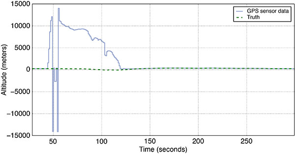
    Several challenges arise when combining multiple sensors in a single navigation system due to specific sensor characteristics. While an accurate navigation solution is obtained by an inertial navigation system with GNSS aiding in open-sky environments, urban canyons and indoor environments degrade the quality of GNSS signals or lead to GNSS outages such that no accurate navigation solution is available.

    On the other hand, laser rangefinder measurements allow for the generation of accurate relative measurements indoors. However, due to the limited range of the laser rangefinder, no or only a few measurements are available outdoors away from buildings. Obviously, it is best to exploit the complementary characteristics of both sensors. To avoid losing information, hard switching between two different navigation systems is undesirable. Hence, two main challenges arise:

    • Accurate time synchronization is necessary when processing measurements from different sensors.
    • A method has to be developed for the decision on whether a measurement should be processed or rejected.

    Moreover, for aerial vehicles, two more requirements must be met:

    • Estimation of the 3D position and attitude instead of only the 2D position and heading as provided by 2D simultaneous localization and mapping (SLAM) approaches.
    • Estimation of the vehicle’s velocity and inertial measurement unit (IMU) biases.

    Our goal was to develop a navigation system that provides an accurate navigation solution for large-scale environments. The navigation system needed to provide a frequent navigation solution at the update rate of the IMU with very short delays. The framework needed to seamlessly integrate GNSS and other sensors such as a laser rangefinder or cameras. Additionally, the approach could not be limited to a specific sensor setup except for a mandatory GPS receiver, necessary for absolute positioning.

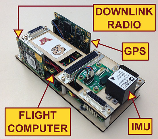
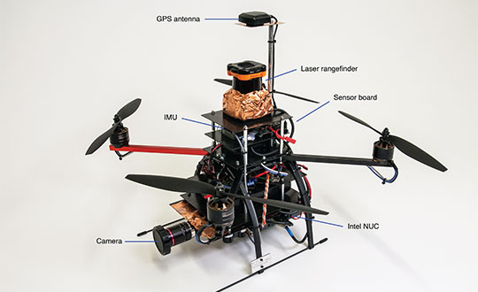
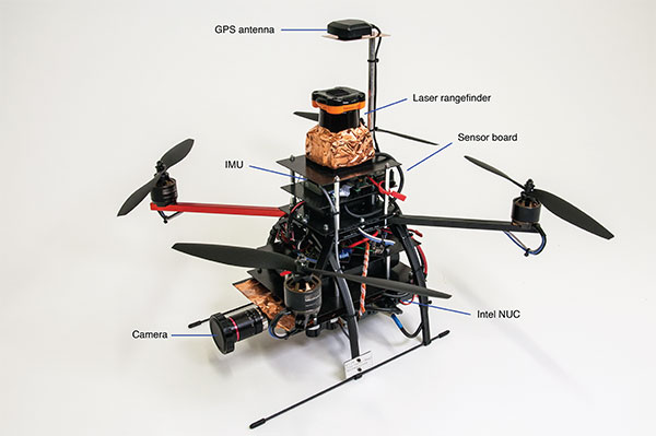
    The results presented in the literature often do not include large-scale, realistic environments. Some investigators only consider short indoor sequences, while others ignore challenging GNSS conditions. In contrast, the focus of our approach is on rejecting outlier measurements in transition zones such as urban-canyon environments occurring between outdoor open sky and indoor environments. The choice of the navigation system architecture depends on the requirements of a specific platform. In the case of a quadrotor helicopter (see FIGURE 1), a high update rate is necessary for vehicle guidance and control. Therefore, we chose a Kalman-filter-based approach because it has the advantage over pure SLAM approaches when providing a navigation solution at a high update rate is required.

    FIGURE 1. Components of the quadrotor helicopter. (Photo: K. Mueller, J. Atman, N. Kronenwett & G.F. Trommer)
    FIGURE 1. Components of the quadrotor helicopter. (Photo: K. Mueller, J. Atman, N. Kronenwett & G.F. Trommer)

    SYSTEM OVERVIEW

    We attached several sensors and two processing platforms to the quadrotor helicopter used in our work. A microcontroller sensor board reads the sensor values from the IMU, digital compass, air pressure sensor and a GPS-only GNSS module. Timestamps are generated for each sensor data type so that accurate synchronization is provided even when delays occur, such as when processing the sensor data. The IMU is mounted close to the center of the vehicle. The air pressure sensor is directly attached to the sensor board, while the three-axis digital compass is attached to the quadrotor’s landing skid to avoid interfering magnetic fields from power electronics. The GPS receiver provides pseudorange and Doppler measurements at a rate of 10 Hz. Moreover, ephemeris data for each satellite and Klobuchar ionospheric parameters are recorded to correct the measurements. Each second, a time pulse is generated by the receiver to precisely determine the time when GPS measurements were taken. Additionally, the time pulse is used to estimate the drift of the real-time clock (RTC) on the sensor board and, therefore, to provide more accurate timestamps.

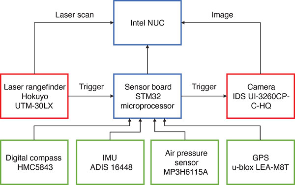
    A two-dimensional laser rangefinder is mounted on top of the helicopter. Distance and angular information of objects within a scan angle of 270° is provided by this sensor. The maximum range is 30 meters. Time synchronization is achieved through a pulse registered by the microcontroller sensor board before every scan. The body of the laser rangefinder is shielded using copper foil to reduce interference with signals received by the GPS antenna. A trigger signal is sent to the camera mounted at the front of the helicopter to provide time synchronization. However, the camera was not used for the results presented in this article. An overview of the sensor setup and time synchronization is depicted in FIGURE 2.

    The camera and laser rangefinder data is sent via USB to a powerful computing platform attached to the bottom carbon-fiber sheet. Time synchronization information and additional sensor data is sent from the microcontroller sensor board to the computer for processing the sensor data and calculating the navigation solution.

    FIGURE 2. Block diagram showing signal flows among system hardware components. (Photo: K. Mueller, J. Atman, N. Kronenwett & G.F. Trommer)
    FIGURE 2. Block diagram showing signal flows among system hardware components. (Photo: K. Mueller, J. Atman, N. Kronenwett & G.F. Trommer)

    NAVIGATION SYSTEM

    The navigation system presented in this article was developed to provide a navigation solution in both outdoor and indoor environments. Therefore, processing GPS position and velocity estimations must be possible, as well as handling of relative position and heading angle changes resulting from the laser rangefinder scans. Challenges arise due to the different time delays as illustrated in FIGURE 3. IMU measurements are available at a high frequency. Messages with the trigger timestamps are sent from the sensor board to the computer to provide information about when a GPS or laser measurement was taken.

    FIGURE 3 Time sequencing of measurements and calculations. (Photo: K. Mueller, J. Atman, N. Kronenwett & G.F. Trommer)
    FIGURE 3 Time sequencing of measurements and calculations. (Photo: K. Mueller, J. Atman, N. Kronenwett & G.F. Trommer)

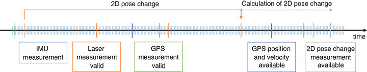
    The corresponding measurements are available with significant delays. Since GPS pseudorange and Doppler measurements are not immediately available and processing requires additional time, the typical delay between the point in time when the measurement was taken by the receiver and the time when the estimated position and velocity are available to the navigation filter is between 70 and 90 milliseconds. Even longer delays occur when processing laser rangefinder data. After processing the laser scans, the horizontal position changes and yaw angle changes (in this article, denoted as two-dimensional pose change measurements) are available for analysis. However, these changes are relative to a point in time in the past. Moreover, due to the processing, additional delay occurs and synchronization with the correct laser rangefinder trigger signal is required. The requirement to process measurements with a temporal overlap causes additional complexity, such as having several GPS measurements that are taken in the time period covered by a pose change measurement.

    Error-State Kalman Filter with Stochastic Cloning. An error-state Kalman filter with 16 states estimates the vehicle’s 3D position, 3D velocity, attitude, accelerometer and gyroscope biases, and the bias for the barometric altimeter. The prediction step of the filter consists of integrating the specific force and angular rate measurements of the IMU. Measurements of the air pressure sensor and the digital compass have negligible delays, so these measurements are processed in the Kalman filter update step without compensating for delays. As we mentioned, the assumption of insignificant delays does not hold for GPS measurements and pose change measurements. Thus, we implemented stochastic cloning to overcome errors that would be introduced by delays. The idea of stochastic cloning is to augment the state vector and covariance matrix by copies of the state and covariance estimates at a specific point in time. As the augmented covariance matrix contains cross-correlation terms between the state at a previous time instance and the current state, processing of delayed measurements corrects the current state and covariance estimations.

    Processing GPS Measurements. The first step when processing GPS measurements is to clone the current filter state. As outlined in the section “System Overview,” the time pulse generated by the receiver is used to determine the time when a measurement is taken. Once the pseudorange measurements are available, corrections are calculated. A weighted least-squares estimation is used to calculate position and velocity. The weight for each pseudorange measurement is the inverse of the estimated variance, which is calculated depending on the carrier-to-noise-density ratio. Weights for Doppler measurements are calculated similarly.

    To reduce the errors introduced by satellite signals of low quality, a minimum carrier-to-noise-density ratio of 33 dB-Hz and a minimum elevation angle of 15° are required for the satellite signals. In addition to position and velocity, valuable information is drawn from the estimation: The variance of the calculated position is chosen to be proportional to the weighted root mean square value of the residuals and the position dilution of precision (PDOP). The velocity variance is calculated similarly. In case only four satellites are used, the variance is only proportional to the PDOP as no residuals are available. The position and velocity estimates are processed by the Kalman filter using these estimated variances. Moreover, before the filter update step is executed, the Mahalanobis distance for each measurement is calculated and outliers removed.

    Additionally, measurements are not processed if their variance is above a threshold. This typically occurs in the vicinity of buildings as non-line-of-sight signals are tracked by the receiver and, therefore, processing these measurements is not desired.

    Laser Rangefinder Processing. As described in the previous section, stochastic cloning is used to treat delayed pose change measurements. To process a measurement, two cloned states are necessary.

    A pose change measurement consists of a relative translation and a rotation, both given in coordinates of the body-stabilized frame, which is identical to the body frame but compensated for roll and pitch angles. Hence, the x and y axes of the body-stabilized frame are parallel to the ground. Several methods could be used for generating pose-change measurements, such as camera-based approaches, laser rangefinder approaches or hybrid approaches. In our work, Cartographer, a laser SLAM approach, is used to obtain horizontal position and yaw angle changes. However, the SLAM module could be easily replaced by other laser SLAM approaches.

    As laser SLAM approaches build an incremental map, the laser’s pose is given with respect to the map frame. Therefore, the translational and rotational components of the pose-change measurement must be transformed from the map frame to the body-stabilized frame before being processed by the Kalman filter. Different options are possible when choosing the first point in time for a relative measurement (the second point in time is determined by the most recent laser measurement).

    We decided to use a keyframe-based aiding technique. A keyframe is defined and the filter state is cloned accordingly. After the processing of a laser measurement by the SLAM algorithm, pose estimations given in map coordinates are transformed to pose change measurements relative to this keyframe. The keyframe is changed depending on the filter status information as outlined in the section “Using the Filter Status Information” of this article. Additionally, the keyframe is changed if the difference between consecutive pose estimations exceeds a threshold. This indicates an erroneous pose estimation by the SLAM module as only small pose changes are expected due to the high update rate of laser scans and the limited velocity of the vehicle. As a result, the influence of errors in the SLAM module on the navigation solution provided by the Kalman filter is reduced.

    FILTER STATUS

    Above, we described how relative and absolute delayed measurements are processed in an error-state Kalman filter. However, simply processing all available measurements will not lead to the best performance of the filter. For example, the laser SLAM algorithm might not provide accurate and reliable results in open-sky environments free from human-made structures, as mainly vegetation is detected by the laser rangefinder.

    To derive a metric for the decision on the necessity of integrating additional relative measurements, we provide a classification scheme based on GPS measurements. The advantage of using only GPS measurements for the filter status determination is the versatility of the approach: A GPS module will be available on almost every platform. The laser rangefinder, however, could be replaced by a camera without modifications in the classification scheme.

    Clearly, processing GPS in indoor environments is not an option as no measurements are available. On the contrary, in outdoor open-sky environments, a sensor setup comprising GPS, IMU, digital compass and air pressure sensor results in an accurate navigation solution. Therefore, the interaction of different sensors in transition phases and urban-canyon environments is the most critical part for an accurate navigation solution in large-scale environments. The following paragraphs introduce the classification of single GPS position measurements and the determination of filter status based on the GPS classification.

    Classification of Single GPS Position Measurements. The first step for the filter status determination is the classification of single GPS position measurements. The categories for a measurement are very good, good, medium and poor. Two parameters are used for the classification: the number of satellites used for the position calculation and the estimated variance. For a very good measurement, at least six satellites are required; for a good measurement, at least five satellites are necessary. Moreover, thresholds for the estimated position variance are applied. As the variance is proportional to the PDOP and the root mean square of the weighted residuals, this means that a very good or good position measurement must offer a good satellite constellation and small residuals.

    Filter Status Determination. The classification of GPS position measurements is used to calculate a filter status. First, a sum over a time interval of one second is computed. The number of positions classified as very good are multiplied by a factor of four, good positions count twice, and the number of medium positions added without a multiplicative factor. In our setup, 10 position measurements are available in one second. The final filter status is determined using two thresholds. If the sum is at least 20, the filter status is “Good GPS.” This means that five measurements classified as being very good or all 10 measurements classified as being good would be sufficient for this status.

    The “Medium GPS” status is achieved with a sum between 10 and 20. If no valid GPS measurements have been available over the last five seconds, an additional indoor flag is set, and it is assumed that the vehicle is now indoors. As soon as GPS position measurements become available again, the filter status is re-calculated. The parameters for the filter status are determined empirically and provide robust results for a large variety of scenarios. However, minor changes of the parameter set to classify single measurements might be necessary in case a different GNSS hardware setup is used.

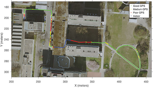
    The resulting filter status for an example trajectory is shown in FIGURE 4. As expected, GPS is good in the western part of the trajectory, and the status quickly deteriorates to poor GPS between the high-rise buildings. Just before entering the building, the status changes to “Indoor.” After leaving the building and moving north, the filter status changes mainly between good and medium GPS as signals are blocked due to buildings or mitigated due to foliage. The end of the trajectory in the eastern part offers better GPS conditions since the surrounding buildings are smaller and the status changes to “Good GPS.”

    FIGURE 4. The filter status changes from “Good GPS” to “Poor GPS” in the vicinity of high buildings and provides important information on how accurately the filter is aided by processing GPS measurements. (Photo: K. Mueller, J. Atman, N. Kronenwett & G.F. Trommer)
    FIGURE 4. The filter status changes from “Good GPS” to “Poor GPS” in the vicinity of high buildings and provides important information on how accurately the filter is aided by processing GPS measurements. (Photo: K. Mueller, J. Atman, N. Kronenwett & G.F. Trommer)

    Using the Filter Status Information. The filter status provides valuable information when combining GPS and relative measurements. As outlined in previous sections, the filter status “Good GPS” occurs in open-sky environments where processing of additional relative measurements does not improve the navigation solution. Since the laser SLAM solution might be corrupted in areas without a sufficient number of human-made structures, relative measurements are not processed while the filter status is “Good GPS.” Additionally, the keyframe is changed in short time intervals during this status. The reasoning behind this decision is that it is desired to have a good estimation of the absolute position and orientation with a low uncertainty at the time a keyframe is chosen.

    During a period with “Good GPS” conditions, position estimation typically becomes gradually better. For the same reason, it is best to retain a keyframe for a long time when the filter status is “Poor GPS” or “Indoor.” In these scenarios the laser SLAM algorithm provides accurate results as the environment mostly consists of human-made structures. A drawback inside buildings is that the Earth’s magnetic field might become distorted, for example close to elevators. Hence, magnetometer measurements are not processed when the “Indoor” flag is set. If the status “Medium GPS” is set, GPS and relative measurements should be weighted equally. The keyframe is retained until a predefined maximum age is reached or inconsistencies in the SLAM solution are detected.

    In contrast to the “Poor GPS” case, the integration of relative measurements is more pessimistic, and the variance is chosen in the range of the typical GPS accuracy. This takes into account that a very accurate laser SLAM solution is not assured. However, the processing of relative measurements improves position accuracy and avoids the growth of filter state covariance, which is beneficial for rejecting faulty measurements. Independent of the filter status, GPS measurements fulfilling the Mahalanobis distance threshold criterion are processed.

    RESULTS

    The results of three trajectories recorded at the campus of the Karlsruhe Institute of Technology are presented in this section. All trajectories cover outdoor environments with good GPS signal reception as well as urban-canyon and indoor sections. Since flying these challenging trajectories was not possible due to legal reasons and due to small doors that had to be passed through, the quadrotor helicopter was manually carried.

    The first trajectory shown in FIGURE 5 starts in an open-sky environment. At position 1, the footpath goes between two 40-meter buildings. Hence, GPS satellite signals are blocked and non-line-of-sight signals are tracked by the receiver that increasingly deteriorate GPS positon and velocity accuracy. The indoor section starts at position 2. After 30 seconds of indoor navigation, the trajectory continues north on the sidewalk. On this section, numbered 4 in Figure 5, a six-story building on the left side and a nearby building on the right side cause medium to poor GPS conditions as was shown in Figure 4. Despite the difficult conditions, the trajectory follows the footpath correctly. Of course, as no GPS correction service or satellite-based augmentation system is used, sub-meter level accuracy is not achieved. At position 2, the trajectory passes along stairs.

    FIGURE 5. Trajectory 1 featuring two high buildings of 42-meter height between positions 1 and 2 in the center of the image. After an indoor section the building is left at position 3. The total time of the trajectory is 394 seconds. (Photo: K. Mueller, J. Atman, N. Kronenwett & G.F. Trommer)
    FIGURE 5. Trajectory 1 featuring two high buildings of 42-meter height between positions 1 and 2 in the center of the image. After an indoor section the building is left at position 3. The total time of the trajectory is 394 seconds. (Photo: K. Mueller, J. Atman, N. Kronenwett & G.F. Trommer)

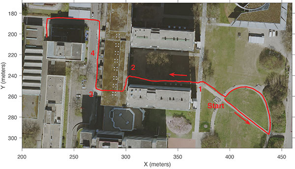
    Therefore, accuracy in the north direction is very good. In the east direction, however, the error is larger as the trajectory should be farther east within the building. This error remains throughout the indoor section until position 3, as no GPS position measurement is processed to correct for the error. After leaving the building, the error in the east direction becomes smaller by processing accurate GPS position measurements. After heading north on the sidewalk, the error is within the expected accuracy bounds specified by the GPS position accuracy. The smoothness of the trajectory after leaving the building shows that the rejection of GPS position outliers leads to a consistent navigation solution.

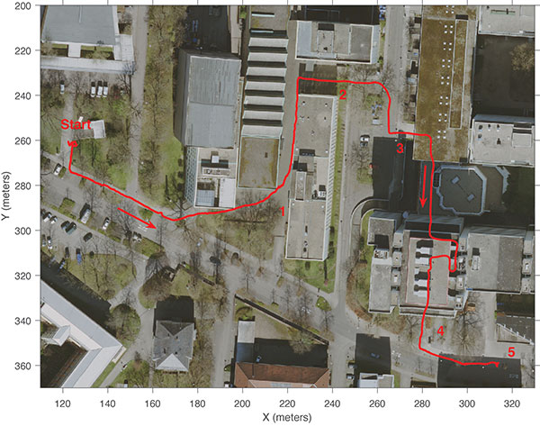
    The second trajectory is the longest of the three trajectories, covering 400 meters in 9 minutes. The first difficult section is denoted by position 1 in FIGURE 6, when the vehicle moves between two buildings. The walls of the right building are covered by metal plates. It looks like the trajectory is very close to the edge of the right building. However, this effect is from the perspective view of the building in the georeferenced image. We passed below a canopy at position 2 and entered a building at position 3. An accurate position solution is available during the long indoor section with multiple turns. The total time spent indoors was 112 seconds. GPS position measurements becoming available after leaving the building at position 4 improve the accuracy of the navigation solution. However, due to the high accuracy of the position estimation before leaving the building, only small filter innovations occur. The trajectory ends on the sidewalk near the building identified as number 5.

    FIGURE 6. Trajectory 2 with a total duration of 9 minutes. An accurate position estimation is obtained during the segment with poor GPS signal reception between positions 1 and 2 and during the indoor section between positions 3 and 4. (Photo: K. Mueller, J. Atman, N. Kronenwett & G.F. Trommer)
    FIGURE 6. Trajectory 2 with a total duration of 9 minutes. An accurate position estimation is obtained during the segment with poor GPS signal reception between positions 1 and 2 and during the indoor section between positions 3 and 4. (Photo: K. Mueller, J. Atman, N. Kronenwett & G.F. Trommer)

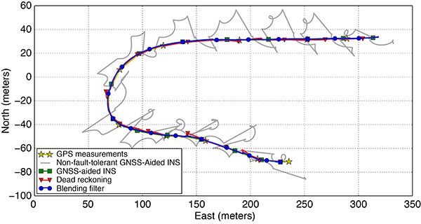
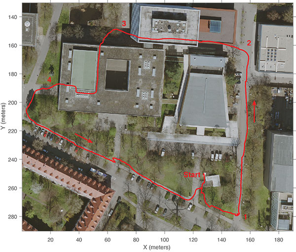
    Trajectory three, shown in FIGURE 7, is the most challenging, with position errors exceeding those of the previous two trajectories. Already at the start of the trajectory, only six GPS satellites can be used for calculating position and velocity estimates. It is several meters until an accurate position estimate is available at position 1. Between positions 2 and 3, a section with buildings up to 56 meters tall results in no accurate GPS position fixes being available for more than 30 seconds. In this section, the computed trajectory clearly is several meters too far north. Additionally, at position 2 the heading change is smaller than 90 degrees, which results in additional drift. Before entering the building at position 3, GPS position measurements become available and the position is corrected, reducing the error in the north. After 57 seconds indoors, we exited the building at position 4. The position solution is still too far north, but is corrected by additional measurements so that good accuracy is achieved when walking on the sidewalk. The trajectory ends at its start position.

    FIGURE 7. Trajectory 3. Poor GPS conditions due to a building of 56-meter height near the north part of the trajectory cause position errors. At position 3 accurate GPS measurements are available and correct the position such that an accurate navigation solution is obtained during the indoor part part of the trajectory. (Photo: K. Mueller, J. Atman, N. Kronenwett & G.F. Trommer)
    FIGURE 7. Trajectory 3. Poor GPS conditions due to a building of 56-meter height near the north part of the trajectory cause position errors. At position 3 accurate GPS measurements are available and correct the position such that an accurate navigation solution is obtained during the indoor part part of the trajectory. (Photo: K. Mueller, J. Atman, N. Kronenwett & G.F. Trommer)

    CONCLUSION

    The navigation system presented in this article fuses GPS measurements and relative pose change measurements to provide an accurate navigation solution in both outdoor and indoor scenarios. We show that position errors are small even for challenging scenarios with high buildings and poor GPS signal reception. Currently, the accuracy in outdoor environments is limited by GPS accuracy. Further improvements are expected by including additional GNSS such as GLONASS or Galileo to obtain better satellite geometry, especially in urban-canyon scenarios.

    MANUFACTURERS

    We used a u-blox LEA-M8T GPS receiver, an Analog Devices ADIS 16448 IMU, a Freescale (now, NXP Semiconductors) MP3H6115A air pressure sensor, a Honeywell HMC5843 digital compass, an Hokuyo UTM-30LX laser rangefinder, an IDS UI-3260CP-C-HQ camera, and an Intel Next Unit of Computing (NUC) platform. We constructed the quadrotor helicopter ourselves. The motors, motor controllers and landing skid are from MikroKopter, while the carbon fiber sheets and the sensor board PCB are our own design. We used a Pixhawk 4 flight controller from Pixhawk.

    ACKNOWLEDGMENTS

    The authors acknowledge financial support from the Federal Ministry of Transport and Digital Infrastructure of Germany in the framework of mFUND. We also thank the City of Karlsruhe for providing the georeferenced orthophotos. The datasets used for the results presented in this article are available on our project website. This article is based on the paper “A Multi-Sensor Navigation System for Outdoor and Indoor Environments” presented at ION ITM 2020, the 2020 International Technical Meeting of The Institute of Navigation, San Diego, California, Jan. 21–25, 2020.


    KARSTEN MUELLER received an M.Sc. from the Karlsruhe Institute of Technology (KIT), Germany, in 2015, after which he started research as a Ph.D. candidate in KIT’s Institute of Systems Optimization.

    JAMAL ATMAN received an M.Sc. in electrical engineering and information technology from KIT in 2015. He is a research engineer in KIT’s Institute of Systems Optimization.

    NIKOLAI KRONENWETT received an M.Sc. degree in electrical engineering and information technology from KIT in 2015. He is a Ph.D. candidate in KIT’s Institute of Systems Optimization.

    GERT F. TROMMER received Dipl.-Ing. and Dr.-Ing. degrees in electrical engineering from the Technical University of Munich, Germany. He is a professor in KIT’s Institute of Systems Optimization.

    FURTHER READING

    • Authors’ Conference Paper

    “A Multi-Sensor Navigation System for Outdoor and Indoor Environments” by K. Mueller, J. Atman, N. Kronenwett and G.F. Trommer in Proceedings of ITM 2020, the 2020 International Technical Meeting of The Institute of Navigation, San Diego, California, Jan. 21–24, 2020, pp. 612–625. https://doi.org/10.33012/2020.17165.

    • Camera and Laser Rangefinder Navigation

    Navigation Aiding by a Hybrid Laser-Camera Motion Estimator for Micro Aerial Vehicles” by J. Atman, M. Popp, J. Ruppelt and G.F. Trommer in Sensors, Vol. 16, No. 9, 2016. https://doi.org/10.3390/s16091516.

    Vision-Based State Estimation and Trajectory Control Towards High-Speed Flight with a Quadrotor” by S. Shen, Y. Mulgaonkar, N. Michael and V. Kumar in Proceedings of Robotics: Science and Systems IX, Berlin, Germany, June 24–28, 2013. https://doi.org/10.15607/RSS.2013.IX.032.

    “Laser Range Finder Aided Indoor Navigation for a Micro Aerial Vehicle” by P. Crocoll, J. Seibold, M. Popp and G.F. Trommer in European Journal of Navigation, Vol. 11, No. 1, pp. 4–14, 2013.

    • Keyframe-Based Navigation

    “Relative Navigation: A Keyframe-Based Approach for Observable GPS-Degraded Navigation” by D.O. Wheeler, D.P. Koch, J.S. Jackson, T.W. McLain and R.W. Beard in IEEE Control Systems Magazine, Vol. 38, No. 4, 2018, pp. 30–48. https://doi.org/10.1109/MCS.2018.2830079.

    • Integrated Navigation

    “3D Multi-Copter Navigation and Mapping Using GPS, Inertial, and LiDAR” by E.T. Dill and M. Uijt de Haag in NAVIGATION: Journal of The Institute of Navigation, Vol. 63, No. 2, Summer 2016, pp. 205–220. https://doi.org/10.1002/navi.134.

    INS/GPS/LiDAR Integrated Navigation System for Urban and Indoor Environments Using Hybrid Scan Matching Algorithm” by Y. Gao, S. Liu, M.M. Atia and A. Noureldin in Sensors, Vol. 15, No. 9, 2015, pp. 23286–23302. https://doi.org/10.3390/s150923286.

    Toward a Unified PNT — Part 1; Complexity and Context: Key Challenges of Multisensor Positioning” by P.D. Groves, L. Wang, D. Walter, H. Martin and K. Voutsis in GPS World, Vol. 25, No. 10, October 2014, pp. 18, 27–34, 49.

    Toward a Unified PNT — Part 2; Ambiguity and Environmental Data: Two Further Key Challenges of Multisensor Positioning” by P.D. Groves, L. Wang, D. Walter and Z. Jiang in GPS World, Vol. 25, No. 11, November 2014, pp. 18, 27-35.

    Principles of GNSS, Inertial, and Multisensor Integrated Navigation Systems, 2nd edition, by P.D. Groves. Published by Artech House, Boston, Massachusetts, 2013.

    • Stochastic Cloning

    “Stochastic Cloning: A Generalized Framework for Processing Relative State Measurements” by S.I. Roumeliotis and J. W. Burdick in Proceedings of 2002 IEEE International Conference on Robotics and Automation, Washington, DC, May 11–15, 2002, pp. 1788–1795. https://doi.org/10.1109/ROBOT.2002.1014801.

  • Robotic Research provides navigation system for GPS-denied areas

    Robotic Research provides navigation system for GPS-denied areas

    Photo: Robotic Research
    Photo: Robotic Research

    Robotic Research will showcase its RR-N-140 navigation system at Booth #407 at AUVSI Xponential 2019, which takes place April 29-May 2 in Chicago.

    The system provides accurate, absolute and relative 3D (six-degrees-of-freedom, or 6 DOF) localization information for ground vehicles of all sizes.

    The device delivers exceptional localization performance in GPS‐denied or compromised areas. It is designed specifically for use on unmanned ground vehicles and is heavily customizable to incorporate a wide variety of sensor inputs into the navigation solution.

    Robotic Research develops and deploys autonomous vehicle innovations for both commercial and government customers.

    Features of the RR-N-140 include:

    • Accurate, real-time navigation/localization solution for wheeled or tracked ground vehicles
    • Adaptable for use on surface vessels
    • Exceptional localization performance in GPS-denied or compromised areas
    • Dual antenna GNSS for zero-speed heading detection and redundancy
    • Rugged IP67 Construction designed to meet shock and vibration environments typical of military vehicles
    • Up to 4X configurable vehicle speed / encoder inputs
    • Configurable GNSS and IMU options allow tailored solutions for all levels of performance
    • Customizable to directly interface with and process a variety of sensor inputs (e.g. LADAR, Stereo and Monocular Cameras, Ultra-Wideband Ranging Radios)
    • Easy integration with the Robotic Research Warfighter Localization family of systems (WarLoc)
    • Web interface for user-level diagnostics and configuration
    • Ethernet, CANbus, and RS-232 Serial Data Interfaces
    • Independent Ethernet ports for separation of navigation solution and sensor processing data
    • Robust Built-in-test (BIT) error reporting during runtime
    • Redundant IMU and GNSS options available for fault-tolerance
    • NTP Server and GPS PPS signals for time synchronization
    • Low SWAP
    • 7.2”L x 6.4” W x 2.9” H
    • 4.0 lbs
    • 22W at 9.5-36 VDC
  • Innovation: Robustness to Faults for a UAV

    Innovation: Robustness to Faults for a UAV

    Integrated Navigation Systems Using Parallel Filtering

    The authors look at the development of a robust navigation system employing a GNSS receiver, accelerometers, gyroscopes, magnetometers, an airspeed device and dead reckoning to supply a blended navigation solution to a flight control system on a small, unmanned aerial vehicle.

    By Trevor Layh and Demoz Gebre-Egziabher

    INNOVATION INSIGHTS by Richard Langley
    INNOVATION INSIGHTS by Richard Langley

    THE NUMBER FOUR has special significance to humankind.  According to Penelope Merritt (a Samuel Beckett scholar) “[f]our has long been a number of completion, stability and predictability, as well as the representation of all earthly things.” And so it is with navigation systems. There are four important requirements of any navigation system: accuracy, availability, continuity, and integrity. To quickly review:

    Accuracy describes how well a measured value agrees with a reference value, typically the true value.

    Availability refers to a navigation system’s ability to provide the required function and performance within the specified coverage area at the start of an intended operation.

    Continuity is the ability of a navigation system to function without interruption during an intended period of operation.

    Integrity refers to the trustworthiness of a navigation system. A system might be available at the start of an operation, and we might predict its continuity at an advertised accuracy during the operation. But what if something unexpectedly goes wrong? If some system anomaly results in unacceptable navigation accuracy, the system should detect this and declare that it can no longer be used for navigation at the expected accuracy level. GPS, for example, has built into it various checks and balances to ensure a fairly high level of integrity. The same may be said of other global navigation satellite systems. Satellite performance is continuously monitored and a satellite is set unhealthy when an anomaly is detected. Some receivers have built-in receiver autonomous integrity monitoring to detect and isolate problematic satellite signals and navigation support systems (such as the Wide Area Augmentation System) independently monitor the health of satellite signals and supply a timely warning in the case of anomalous signal behavior.

    However, an aircraft, vessel, vehicle or some other platform still needs to be able to navigate if an independent primary navigation system becomes unavailable. This requires a back-up system of some kind and may take the form of an inertial navigation system, another radionavigation system such as eLoran, celestial navigation or just dead reckoning. Ideally, the platform’s navigation system should have multiple integrated sensors so that it continues to operate seamlessly even in the event of a sensor failure. We would call such a system robust. While we often use this word to describe a person with a strong healthy constitution, we can apply it to systems to refer to their ability to tolerate perturbations that might affect their functionality. A robust navigation system employs multiple sensors and uses appropriate filtering systems to autonomously detect anomalies, such as a failed sensor, and then to isolate it from the combined navigation solution.

    It is important to catch navigation sensor failures early, ideally instantaneously, to reduce integrity risk as much as possible. This is not a trivial operation, and it requires clever software design and operation.

    In this month’s column, we look at the development of such a robust navigation system employing a GNSS receiver, accelerometers, gyroscopes, magnetometers, an airspeed device and dead reckoning to supply a blended navigation solution to a flight control system on a small, unmanned aerial vehicle.

    While the number four has special significance in religion, science and other aspects of our lives, the number five may be considered equally important — denoting, for example, how many digits we have on our hands and feet. For those mathematically inclined, it is the first safe prime number. And perhaps we should use it to more fully characterize a navigation system, denoting its accuracy, availability, continuity, integrity and robustness.


    “Innovation” is a regular feature that discusses advances in GPS technology and its applications as well as the fundamentals of GPS positioning. The column is coordinated by Richard Langley of the Department of Geodesy and Geomatics Engineering, University of New Brunswick. He welcomes comments and topic ideas. Email him at lang @ unb.ca.


    Multi-sensor navigation systems generate an estimate of a vehicle’s state vector by fusing information from a disparate set of sensors. In many instances the sensors used in these systems provide redundant information. For example, in GNSS receivers, more than four (the minimum number required) satellite measurements are used to generate a position, navigation and time or PNT solution. This redundancy is beneficial because it enhances accuracy. It also enhances integrity or robustness because it allows the detection and possibly the isolation of failed sensors. However, fault detection and isolation schemes do not work instantaneously because once a sensor has failed, it takes some time before this can be detected. This is especially true for failures that are drift-like in nature as opposed to step-like. Drift-like errors grow slowly and, thus, fault detection schemes that monitor filter residuals cannot detect them until they have grown to a point where they are sufficiently large to exceed preset thresholds.

    The time between the onset of a fault and its detection — called the detection time — depends on the fault magnitude and thresholds of the fault detection algorithms. For a given fault magnitude, the length of the detection time represents a compromise between a navigation system’s continuity performance (or false alarm rate) and integrity risk (missed detection probability). The fact that faults cannot be detected instantaneously is an issue particularly for systems that have some form of dead reckoning (such as inertial navigation or velocity-based odometry) integrated with aiding sensors such as GNSS or radars. A failure in the aiding system (for example, a pseudorange fault in GPS) will lead to a corruption of the dead-reckoning solution. Once the GNSS fault has been detected and subsequently removed, the error induced by this failure has already propagated into the dead-reckoning solution. How does one deal with these types of errors? In this article, we discuss a solution to this challenge, which we call parallel filtering.

    Solutions for dealing with the problem exist. For example, one approach that has been used is based on the idea of delayed measurements. In this approach, integration of aiding sensor measurements in the navigation solution is delayed until a period equal to the fault detection time has elapsed. If no faults are detected during this period, then the delayed measurements are extrapolated forward in time and integrated into the navigation solution. Alternately, we can rewind the dead-reckoning solution backwards in time, integrate the delayed measurements and fast-forward the integrated solution up to the current time epoch. While this approach works, it has several shortcomings, of which we will mention just two. First, it requires buffering sensor data. Second, the most current navigation solution is not as accurate as it can be, because it does not incorporate the most recent sensor measurements (that is, the delayed measurements). The parallel filtering approach and fault tolerance we describe in this article deals with both of these shortcomings. Of course, like any other engineering solution, it represents a compromise between competing requirements. We will discuss these compromises and their impacts later in the article. For now, we will concentrate on describing the mechanics of parallel filtering and its performance when implemented in an integrated flight control system used for navigation, guidance and control of small unmanned aerial vehicles or UAVs.

    Parallel Filtering

    To understand parallel filtering, consider the schematic in FIGURE 1, which represents the conventional way in which an integrated navigation system fuses the information from N sensors. All the measurements from the N sensors are integrated in a single sensor-fusion algorithm. In the context of what we are describing here, the algorithm consists of a navigation filter and a fault-detection filter. The sensor-fusion algorithm integrates the measurements from all N sensors and generates a single, optimal estimate of the navigation state vector.

    FIGURE 1. Conventional (centralized) sensor fusion architecture.
    FIGURE 1. Conventional (centralized) sensor fusion architecture.

    In contrast to this, the schematic shown in FIGURE 2 is the parallel filtering approach introduced in this article. In this case, the same N sensors are divided up into M separate sensor clusters.

    FIGURE 2. Parallel filtering architecture.
    FIGURE 2. Parallel filtering architecture.

    The measurements from the sensors in the jth cluster is processed in a sensor-fusion algorithm to generate an estimate of the state vector denoted xj and a covariance matrix Pj. Each pair (xj, Pj) is then sent to a blending filter that generates a single optimal estimate Inn-x and P. The estimate  is a weighted sum of the estimates from the M filters:

    Inn-E1  (1)

    where Bj are blending weights that function as switches, which can be “opened” (set to zero) to isolate a parallel filter momentarily or permanently when a failed sensor is detected. The analogy with a physical switch should not be taken literally, however, because they are not “hard on-off” switches. Instead, they are matrices, which serve to change the emphasis put on a particular parallel filter. The blending weights are calculated so that the estimate Inn-x is an unbiased minimum-variance estimate. In mathematical terms, this means that they minimize the trace of the final covariance P. We will give more detail on how to calculate the weights shortly, but before we do that, let us describe, at a high level, how all of this works.

    Consider that one of the sensors in the Inn-lth cluster fails. TheInn-lth fault detection filter will identify the fault and try to isolate it. If the fault is non-isolable, the Inn-lth fault detection filter will raise an alarm. This can be done in various ways including inflation of the Inn-lth filter covariance Inn-Pl. An increasing covariance matrix Inn-Pl leads to a decreasing value of the corresponding blending weight Inn-Bl . For a non-isolable fault, Inn-Bl  will eventually approach zero, which effectively isolates the Inn-lth cluster from the navigation solution. If the fault was just a momentary glitch, then Inn-x and Inn-xl  are reset. In the simplest case, Inn-xl  can be reset to a weighted sum of remaining M-1 parallel state estimates. This is then blended with all of the other parallel estimates for generating the new Inn-x. This does not require setting aside buffers to store delayed measurements. Neither does it require rewinding the solution back in time when recovering from a faulted sensor scenario.

    Mathematical Formulation

    Providing a detailed derivation of the parallel filter is beyond the scope of this short article. Instead, we will just summarize the steps in the parallel filtering algorithm with the key formulas that are used in determining the blending weights. For simplicity, we will assume that we are working with a system with two parallel filters (M = 2 in Figure 2). How this extends to systems with more parallel filters or complex interlinking between the filters will become apparent later in the article when we present the results from a case study.

    To start, let us define some notation. We assume that the two parallel filters are extended Kalman filters (EKFs) generating estimates of the state vectors x1 and x2. We will denote these estimates Inn-x1 and Inn-x2. The covariances for these estimates are denoted by P1 and P2, respectively. The output of the blending filter is an estimate of the state vector x, which is a subset of x1 and x2. In mathematical terms, this means that we can define two mapping matrices M1 and M2 whose entries are either “1” or “0” and:

    Inn-E2   (2)

    The output of the blending filter Inn-x is, thus, given by:

    Inn-E3. (3)

    The blending weights are computed from:

    Inn-E4  (4)

    Inn-E5  (5)

    where

    Inn-E6  (6)

    Inn-E7 (7)

    Inn-E8. (8)

    The covariance of Inn-x is given by:

    Inn-E9(9)

    where Inn-E9b  and Π is given by:

    Inn-E10(10)

    where P12 is the cross-correlation between the states of parallel filter #1 and #2. We will say more about this shortly. In the meantime, note that in Equation (9), P1 and P2 are the covariances computed by the parallel filters after the measurement update. This computation requires knowledge of K1 and K2, which are the EKF gains for parallel filters. The matrices H1 and H2 are the observation matrices for filters #1 and #2. They relate the measurements y1 and y2 of the two parallel filters to their respective state vectors as follows (refer to Figure 2):

    y= H1x1 + v1   (11)

    y= H2x2 + v2  (12)

    where v1 and v2 are the measurement noises. Thus, the blending filter has to have knowledge of the measurement model and the gains of each parallel filter.

    Finally, note that P12 is zero if the dynamic models (time update equations) for the two parallel filters are completely independent. However, if they share sensors then there will be a correlation and P120. This is the case for the example we present later in this article. In this case, P12 needs to be propagated between measurement updates. This can be done with the covariance time update equation (Lyapunov equation) for the joint state vector

    Inn-joint.

    Note that the architecture depicted in Figure 2 is meant to be a high-level depiction of the idea of parallel filtering. It should not be interpreted as an actual system architecture schematic. This will become apparent in the case study we present later in this article. The system we will consider there consists of three filters of which two are run in series (cascaded so that the output of the first is the input of the second) and each, in turn, is run in parallel with the third filter.

    It is important to note that the proper blending of the various filters’ outputs hinges on an accurate estimate of the individual covariances. This is particularly true when a fault has occurred. An individual filter that has detected a failed sensor must inflate its covariance to reflect its faulted state. How a filter does this is the problem of fault-detection filter design and is beyond the scope of this short article. For the work presented here, we used fault-detection filters, which monitored the EKF measurement residuals to detect sensor faults. When these filters detected a fault, they immediately inflated the faulted sensor’s output noise covariance matrix. We cannot overemphasize, therefore, the importance of having a well-designed fault-detection filter that responds in a timely and accurate manner to sensor faults.

    Case Study: Small UAV Flight Control

    detection/isolation scheme described above, we discuss the results of a blending filter, which was used on the University of Minnesota UAV Laboratory Goldy flight control system (FCS) shown in FIGURE 3. The Goldy FCS is used for navigation, guidance and control of small UAVs. The results presented below were obtained by post-processing flight test data.

    FIGURE 3. Goldy flight control system.
    FIGURE 3. Goldy flight control system.

    The architecture of the parallel filtering scheme used is shown in FIGURE 4. There are three separate filters whose outputs are blended: a GNSS-aided inertial navigation system (INS) filter, an attitude heading reference system (AHRS) filter and an airspeed-based dead-reckoning (DR) filter. Two blending filters are used to fuse the outputs from these three filters. The first blending filter fuses the attitude estimates from a GNSS-aided INS and an AHRS. The second blending filter fuses the position solutions from the GNSS-aided INS and the airspeed-based DR system. The AHRS and the airspeed-based DR filters are a pair of filters, which are cascaded to generate an estimate of the UAV navigation state vector. Thus, in the case of GNSS-denied operations, it can provide a position, velocity and attitude estimate to the flight control system. All of the sensors and software required to run these filters are part of the Goldy FCS. Before we present results of the parallel filter’s performance, we will briefly describe these three systems below.

    FIGURE 4. Goldy parallel filtering architecture. The three-axis magnetometer (Mag.) feeding the attitude heading reference system (AHRS) filter is part of the inertial measurement unit (IMU) device. The device’s accelerometer and gyro outputs feed both the GNSS-INS and AHRS filters. A pitot tube device supplies airspeed measurements to the airspeed-based dead-reckoning (DR) filter.
    FIGURE 4. Goldy parallel filtering architecture. The three-axis magnetometer (Mag.) feeding the attitude heading reference system (AHRS) filter is part of the inertial measurement unit (IMU) device. The device’s accelerometer and gyro outputs feed both the GNSS-INS and AHRS filters. A pitot tube device supplies airspeed measurements to the airspeed-based dead-reckoning (DR) filter.

    The GNSS-aided INS uses a consumer/automotive grade inertial measurement unit (IMU) to generate a position, velocity and attitude solution at a rate of 50 Hz. A 1-Hz measurement update from GPS is used to arrest drift errors inherent in inertial navigation systems, especially those mechanized using low cost consumer/automotive grade sensors. The GPS position updates also allow estimation of the inertial sensor biases. The state vector for this GNSS-aided INS is denoted x1 and consists of the following 15 states: latitude (Λ), longitude (λ), altitude (h), north velocity (Vn), east velocity (Ve), down velocity (Vd), roll angle (φ), pitch angle (θ), yaw angle (ψ), three gyro biases (bp, bq and br) and three accelerometer biases (bax, bay and baz).

    The second and third filters are a pair of estimators connected in series. The AHRS filter generates attitude estimates, which are fed to the airspeed-based DR filter. The AHRS uses the same IMU as the GNSS-aided INS to estimate roll (φ), pitch (θ) and yaw (ψ) attitude states of the vehicle as well as the three gyro biases (bp, bq and br). This AHRS filter’s six-dimensional state vector is denoted x2. The attitude is then used to resolve airspeed measurements from the body frame of the UAV to the north-east-down coordinate frame. After adding an estimate of the local winds to this, a single integration yields a position solution. This is done at a rate of 50 Hz. A periodic 1-Hz update from GPS is used to arrest the inherent DR drift. It also allows estimation of the magnitude of the local winds. The state vector of the airspeed-DR is denoted x3 and consists of the following 11 states: latitude (Λ), longitude (λ), altitude (h), local north wind speed (Wn), local east wind speed (We), yaw angle offset (Δψ), pitch angle offset (Δθ), three airspeed-measurement biases (Ub, Vb and Wb), and altitude offset (Δh).

    In the UAV flight control system, the blended states of interest are position (Λ, λ and h) and attitude (φ, θ and ψ). This implies that four mapping matrices are required for the fusion. First, matrices are needed for the attitude blending using the GNSS-aided INS (M1a) and the AHRS (M2). Then, additional matrices are needed for the position blending using the GNSS-aided INS (M1b) and the airspeed-based DR (M3). The shaping matrices are given by:

    Inn-E13   (13)

    Inn-E14   (14)

    Inn-E15   (15)

    Inn-E16   (16)

    where Ij×k is a j × k identity matrix and Zj×k is a j × k matrix of zeros.

    Filter Performance

    Validation of the parallel filtering scheme was accomplished by post-processing data from a series of flight tests where the Goldy FCS was installed on a UAV flying around a box-shaped trajectory.

    The first set of results was from a case where GPS was available from the moment the FCS is turned on until shortly after takeoff. Thus, GPS was available during initialization, take off roll and initial climb of the UAV. Then, GPS services were interrupted for a three-minute period during flight and restored shortly before the UAV landed. The GPS interruption was simulated by cutting out the 1-Hz measurement updates to the GNSS-aided INS and the AHRS/airspeed-DR system. In the background, however, there was another GNSS-aided INS that had an uninterrupted GPS service throughout the entire flight. This additional GNSS-aided INS solution is referred to as the reference solution and is used as ground-truth for assessing the performance of the parallel filtering scheme. For example, error plots shown below were generated by taking the difference between the various filtering schemes under consideration and this reference solution.

    FIGURE 5 shows the errors in the attitude of all three filters during this flight test. It shows that the blended estimates of heading, pitch and roll tend to oscillate closer to zero error than either of the individual filters themselves. This is reflected in TABLE 1, where it can be noted that the root-mean-square (RMS) error of the blended solution is lower than either the GNSS-aided INS or the AHRS in each of the three attitude solutions.

    FIGURE 5. Attitude errors. The gray vertical lines indicate when GPS availability was interrupted and then restored.
    FIGURE 5. Attitude errors. The gray vertical lines indicate when GPS availability was interrupted and then restored.
    Table 1. RMS orientation errors of different solutions (in degrees).
    Table 1. RMS orientation errors of different solutions (in degrees).

    FIGURE 6 shows the position errors of all three systems and illustrates one of the primary advantages of the proposed architecture. FIGURE 7 and FIGURE 8 show the blending weights matrices B1 and B2 before, during, and after the GPS outage. What is shown in these figures are the diagonal elements of these matrices.

    FIGURE 6. Position errors during a GPS outage.
    FIGURE 6. Position errors during a GPS outage.
    FIGURE 7. Attitude blending weights.
    FIGURE 7. Attitude blending weights.
    FIGURE 8. Position blending weights.
    FIGURE 8. Position blending weights.

    The INS exhibits extreme drift errors after only three minutes of unaided operation. The blending algorithm detects this inaccuracy and places more weight on the slow-drifting AHRS-DR solution, as shown in Figure 8. When GPS services are restored, the GNSS-aided INS error is “reset,” and the position weights are re-established to their pre-outage levels with minimal transient responses.

    We next show data from another flight test where an unplanned but fortuitous fault in the GPS sensor occurred. The cause of this fault has not been definitively determined, but potential reasons for it include loose cabling or outdated firmware. Nevertheless, this fault provided useful flight data for our architecture as no fictitious or simulated data was used. FIGURE 9 shows the GPS altitude measurements during this flight test. At t = 44 seconds a large oscillatory GPS error occurred. Similar errors were present in the GPS measurements of the velocities, latitude and longitude.

    FIGURE 9. GPS sensor errors during a fault.
    FIGURE 9. GPS sensor errors during a fault.

    Thus, all filters were initialized and operated correctly for the first 44 seconds. Between 44 and 132 seconds, the GPS receiver output was in error. This time period corresponds to the taxi, takeoff and initial climb phase of the UAV’s flight. A “reference” GNSS-aided INS, which did not employ the fault detection and isolation scheme that was employed in the parallel filtering system, was running in real time for this flight test. However, the UAV was under manual control (fortunately). As shown by the gray solution in FIGURE 10, the “reference” (non-fault-tolerant) system running in the background diverged and never converged.

    FIGURE 10. Attitude solution during an actual GPS sensor failure.
    FIGURE 10. Attitude solution during an actual GPS sensor failure.

    The dark traces in Figure 10 show the performance of the fault detection and isolation algorithm paired with the parallel filtering scheme described in this article. It is seen to be fault-tolerant and ignores the invalid measurements. Although nearly no aiding was provided until after the GPS sensor converged back to a stable state, the fault tolerant filter provided a much more accurate solution.

    A bird’s eye view of the ground track of the UAV shows a similar trend. This can be seen in the position plot of FIGURE 11, which shows a roughly 60-second segment of the flight.

    FIGURE 11. GPS sensor failure performance: north vs. east.
    FIGURE 11. GPS sensor failure performance: north vs. east.

    This north vs. east plot demonstrates that a non-fault-tolerant GNSS-aided INS provides an unstable position solution similar to the attitude shown in Figure 10. By contrast, the fault-tolerant system described in this article provides a smooth position estimate that ignores the “bad” GPS measurements and tracks the “good” measurements after they convergence back to the truth. Therefore, the safety of the aircraft would not have been in question, and the UAV could have completed multiple segments of fully autonomous waypoint navigation in spite of the faulty sensor measurements provided earlier.

    Summary

    The parallel filtering approach discussed in this article has the potential for providing a systematic way of designing multi-sensor navigation systems, which are robust to sensor faults. Unlike prior approaches, it obviates the need to maintain data buffers to store data, which can be played back in the event of a sensor fault. As noted earlier, like any engineering solution to problems, this one is a comprise between many competing requirements. As such, it has some drawbacks when compared to traditional approaches. We note two of them here as they are the focus of ongoing work. First, the computational overhead associated with this approach can be high especially if a large number of parallel filters are used. Thus, methods for streamlining the computations so that they are not computer-resource intensive will be important.

    The second issue that needs further exploration is the way in which blending weights are computed. A key input to calculating the weights (as well as the “triggers” for the fault detection and isolation algorithm) are the covariances estimated by the various parallel filters. This can be problematic if the covariances used by the parallel filters do not match the true statistics. This can lead to turning off a particular filter when no faults had occurred or, worse, retaining a filter with a failed sensor in the blended solution.

    For more detail about the Goldy FCS, go to www.uav.aem.umn.edu.

    Acknowledgments

    This article is based, in part, on the paper “A Fault-Tolerant, Integrated Navigation System Architecture for UAVs” presented at ION ITM 2015, the 2015 International Technical Meeting of The Institute of Navigation, Dana Point, Calif., January 26–28, 2015. The contents of this article reflect the views of the authors, who are responsible for the facts and the accuracy of the information presented herein. The authors acknowledge the United States Department of Homeland Security for supporting the work reported here through the National Center for Border Security and Immigration under grant number 2008-ST-061-BS0002. However, any opinions, findings, conclusions or recommendations in this article are those of the authors and do not necessarily reflect views of the United States Department of Homeland Security.

    Manufacturers

    The Goldy FCS uses a Hemisphere GNSS Crescent OEM board and an Analog Devices ADIS16405 iSensor MEMS inertial measurement unit.


    Trevor Layh is a M.S. candidate in the Department of Aerospace Engineering and Mechanics at the University of Minnesota in Minneapolis. He obtained his B.S. in mechanical engineering from South Dakota State University, Brookings, S.D., and his research interests include backup navigation systems to GPS-aided inertial navigation systems.

    Demoz Gebre-Egziabher is an associate professor in the Department of Aerospace Engineering and Mechanics at the University of Minnesota. His research focuses on the design of multi-sensor navigation systems. He holds a Ph.D. in aeronautics and astronautics from Stanford University, Stanford, Calif.

    FURTHER READING

    • Authors’ Conference Paper

    “A Fault-Tolerant, Integrated Navigation System Architecture for UAVs” by T. Layh and D. Gebre-Egziabher in Proceedings of ITM 2015, the 2015 International Technical Meeting of The Institute of Navigation, Dana Point, Calif. January 26–28, 2015, pp. 702–712.

    • Attitude Heading Reference System and Airspeed-Based Dead Reckoning Filters

    Correlated-Data Fusion and Cooperative Aiding in GNSS-Stressed or Denied Environments by H. Mokhtarzadeh, Ph.D. dissertation, University of Minnesota UAV Laboratories, 2014.

    “A Recovery System for SUAV Operations in GPS-Denied Environments Using Timing Advance Measurements” by T. Layh, J. Larson, J. Jackson, B. Taylor and D. Gebre-Egziabher in Proceedings of ITM 2015, the 2015 International Technical Meeting of The Institute of Navigation, Dana Point, Calif. January 26–28, 2015, pp. 293–303.

    • UMN UAV Research Lab and Goldy Flight Control System

    Infrastructure” website, University of Minnesota UAV Laboratories, July 2014.

    • Navigation in GPS-Denied Environments

    Impact and Mitigation of GPS-Unavailability on Small UAV Navigation, Guidance and Control by D. Gebre-Egziabher and B. Taylor, Technical Report 2012-2, University of Minnesota, Department of Aerospace Engineering and Mechanics, November 2012. Available through online request.

    • Avionics Reliability

    Introduction to Avionics Systems, 2nd Edition, by R.P.G Collinson. Published by Kluwer Academic Publishers, Boston, Mass., 2003.

    Civil Avionics Systems by I. Moir and A. Seabridge. AIAA Education Series. Published by American Institute of Aeronautics and Astronautics, Reston, Va., 2003.

    • Example of a Fault-Tolerant Avionics System

    “Performance of Honeywell’s Inertial/GPS Hybrid (HIGH) for RNP Operations” by  C. Call, M. Ibis, J. McDonald and K. Vanderwerf in Proceedings of PLANS 2006,  the Institute of Electrical and Electronics Engineers / Institute of Navigation Position, Location and Navigation Symposium, Coronado (San Diego), Calif., April 25–27, 2006, pp. 244–255, doi: 10.1109/PLANS.2006.1650610.

    • GNSS Integrity

    Digging into GPS Integrity: Charting the Evolution of Signal-in-Space Performance by Data Mining 400,000,000 Navigation Messages” by L. Heng, G.X. Gao, T. Walter and P. Enge in GPS World, Vol. 22, No. 11, November 2011, pp. 44–49.

    Integrity for Non-Aviation Users: Moving Away from Specific Risk” by S. Pullen, T. Walter and P. Enge in GPS World, Vol. 22, No. 7, July 2011, pp. 28–36.

    The Integrity of GPS” by R.B. Langley in GPS World, Vol. 10, No. 3, March 1999, pp. 60–63.

    • Multi-Sensor Systems

    Toward a Unified PNT — Part 1: Complexity and Context: Key Challenges of Multisensor Positioning” by P. D. Groves, L. Wang, D. Walter, H. Martin and K. Voutsis in GPS World, Vol. 25, No. 10, October 2014, pp. 18, 27–34, 47–49.

    Toward a Unified PNT — Part 2: Ambiguity and Environmental Data: Two Further Key Challenges of Multisensor Positioning” by P. D. Groves, L. Wang, D. Walter and Z. Jiang in GPS World, Vol. 25, No. 11, November 2014, pp. 18, 27–35.