It’s the beginning of 2022 and the new, modernized NSRS is only about three years away. Hopefully, everyone has been reading NGS’s blueprint documents updated during 2021, and participating in NGS’s webinar series. Together, they provide the latest information about the changes from the existing NSRS to the new NSRS.
My previous columns highlighted many aspects of the new geometric reference frame and geopotential datum. In this month’s column, I will highlight the time-dependent aspect of the modernized NSRS and why it is necessary for the new system.
As I stated before, NOAA’s National Geodetic Survey (NGS) is developing models and tools for users to be able to transform coordinates between the four national terrestrial reference frames and the International Terrestrial Reference Frame, the Geopotential Datum and the North American Vertical Datum of 1988 (NAVD 88), as well as estimate coordinates at epochs different from the survey observation epoch by accounting for movement.
What does NGS mean by estimate coordinates at epochs different from the survey epoch, and why is it necessary to account for movement for the new, modernized NSRS? This column will address these issues.
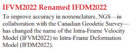
NGS’s January 2022 (Issue 27) edition of NSRS Modernization News announced a paper about the modernized NSRS and a change in name to the Intra-Frame Velocity Model (IFVM). See the box below. Users can sign up for these newsletters here, and can obtain access to previous newsletters here.
The Latest Issue of
|
The new paper was published in October 2021 and is titled “The Mathematical Relation between IFVM2022 as Expressed in ITRF2020 with IFVM2022 as Expressed in the Four Terrestrial Reference Frames of the Modernized NSRS with Dependence on EPP2022.” It can be downloaded here.
The paper describes the mathematical relationship between the Intra-Frame Velocity Model (IFVM2022) and the Euler Pole Parameters (EPP2022).
The NSRS Modernization News announcement states that the IFVM2022 name has been changed to the Intra-Frame Deformation Model (IFDM2022). The latest version of blueprint 1 and the October 2021 (NOS NGS 90) report were published before the name changes, so they refer to IFVM2022 instead of IFDM2022.
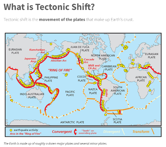
Why is it necessary to account for movement? Coordinates basically change because the Earth’s surface is moving due to the movement of major tectonic plates. See the box below for information about why it is called plate movement or tectonic shift. NGS understands this and is attempting to manage the changing coordinates by providing a time-dependent component.
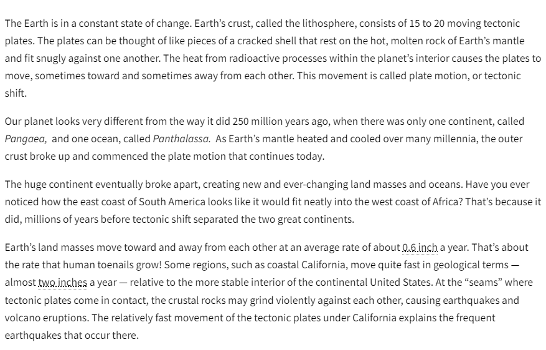
NGS will be defining the following four geometric terrestrial reference frames that are based on the tectonic plates (see map below):
- North American Terrestrial Reference Frame of 2022 (NATRF2022)
- Pacific Terrestrial Reference Frame of 2022 (PATRF2022)
- Caribbean Terrestrial Reference Frame of 2022 (CATRF2022)
- Mariana Terrestrial Reference Frame of 2022 (MATRF2022)
Four Tectonic Plates Part of NGS’s New NSRS
|
As previously stated, NGS is developing models and tools for users to be able to transform coordinates between the four national frames and the International Terrestrial Reference Frame, as well as estimate coordinates at epochs different from the survey observation epoch by accounting for movement. These models are denoted as EPP2022 and IFDM2022.
So, what are EPP2022 and IFDM2022? And what does this mean to surveyors and mappers?
EPP stands for Euler pole parameters (a way of describing a plate’s rotation) and IFDM2022 is a way of computing the drift in coordinates.
Why Euler Pole? See the box titled “Who was Euler?”
Who was Euler?Leonhard Euler was a Swiss who lived in the 1700s. He was one of the greatest mathematicians that ever lived and has been called the greatest mathematician of the 18th century. He founded the studies of graph theory and topology, and made pioneering and influential discoveries in many other branches of mathematics such as infinitesimal calculus. He introduced a lot of modern mathematical terminology and notation, including the notion of a mathematical function. He is also known for his work in mechanics, fluid dynamics, optics, astronomy and music theory. The definition of Euler’s fixed point theorem states that any motion of a rigid body on the surface of a sphere may be represented as a rotation about an appropriately chosen rotation pole, called a Euler pole. This theorem has been used by geologists to understand and describe the motions of tectonic plates. |
NGS’s 2021 revised Blueprint 1, NOAA Technical Report NOS NGS 62, Blueprint for the Modernized NSRS, Part 1: Geometric Coordinates and Terrestrial Reference Frames provides an explanation of Euler poles and “plate-fixed” frames. As stated in the “Who was Euler?” box, the definition of Euler’s fixed-point theorem states that any motion of a rigid body on the surface of a sphere may be represented as a rotation about an appropriately chosen rotation pole, called a Euler pole. The following is stated in the NOS NGS 62 report under “Plate-Fixed Frames and Euler Poles,” section 4:
When considering only the rigid (not deforming) part of a tectonic plate, the horizontal motion of the plate (relative to a global plate-independent reference frame, like the ITRF) can be modeled as a rotation about a geocentric axis passing through a fixed point on Earth’s surface. Although such models must make certain assumptions (such as the rigidity of the plate), the dominant motion of the majority of points on most tectonic plates is the rotation about a fixed point. That point is known as an “Euler pole.”
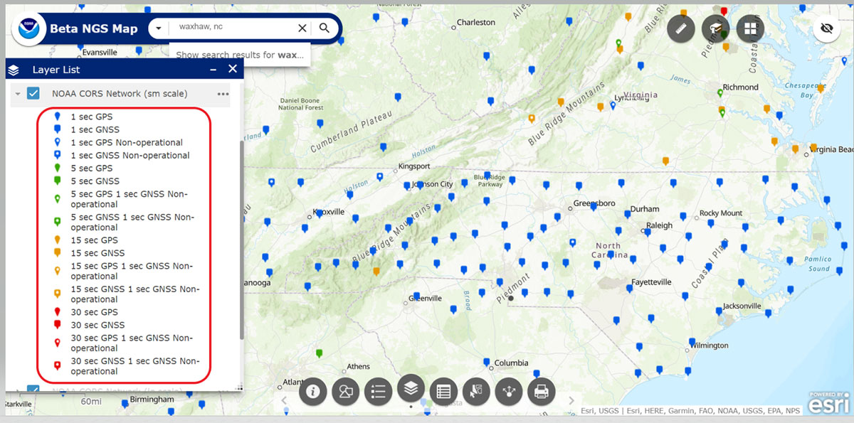
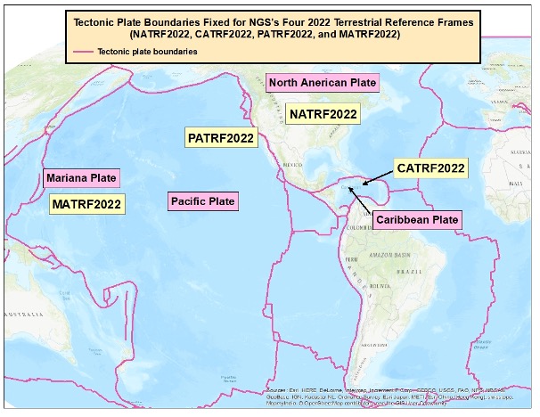
What is important to know is that the determination of a plate’s Euler pole location and the angular velocity with which the plate rotates can be empirically determined using GNSS observations from a CORS network distributed throughout the plate. Figure 1 from the NOS NGS 62 report provides a plot of the North American plate Euler pole and the vectors of the horizontal velocities at select CORS (see the box titled “Figure 1 from NOS NGS 62”).
Figure 1 from NOS NGS 62
Every place on Earth is moving. That includes neighboring marks on the same tectonic plate. What this means is that after the Eulerian motions are removed, the remaining motions left over change the relative differences in coordinates of neighboring marks located on the same tectonic plate. Figures 2 and 3 from the NOS NGS 62 report provide plots of estimates of these remaining velocities (see the boxes titled “Figure 2 from NOS NGS 62” and “Figure 3 from NOS NGS 62.”)
Figure 2 is a plot of the non-Eulerian motions east of 110° west longitudes. As stated in the report, most of the velocities are less than 2 mm/year. The concept is that the EPP2022 and IVDM2022 models will remove the Eulerian and non-Eulerian movement of the marks.
Figure 2 from NOS NGS 62
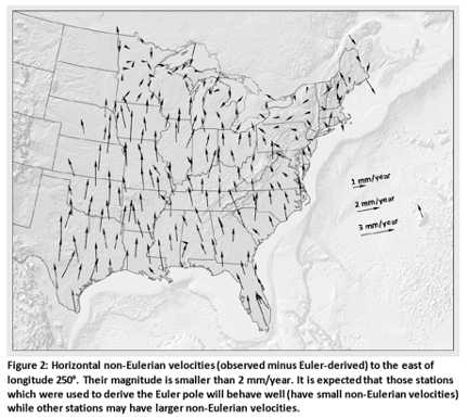
Figure 3 is a plot of non-Eulerian vectors west of 110° west longitude. As indicated in the plot, the large vectors in Western California, Western Oregon and Western Washington show areas of deformation near plate boundaries that don’t appear to be adequately captured just from the North American plate rotation.
Figure 3 from NOS NGS 62
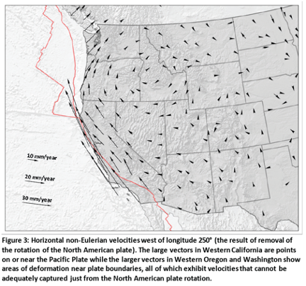
It should be noted that the size of the vectors on Figures 2 and 3 depict a different magnitude of movement. Figure 2 depicts vectors at 1-3 mm/year and Figure 3 depicts movement at 10-30 mm/year.
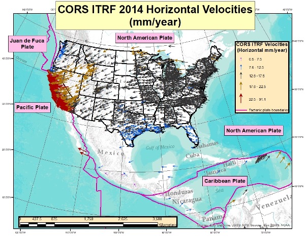
To better visualize the potential size of the movement, I downloaded the CORS ITRF2014 coordinates and velocities from NGS’s website and compiled the results. See the boxes titled “CORS ITRF 2014 Horizontal Velocities” and “Table of ITRF 2014 Horizontal and Upward Velocities of U.S. CORSs.”
CORS ITRF 2014 Horizontal Velocities
Computed Velocities Only (Downloaded Jan. 13, 2022)
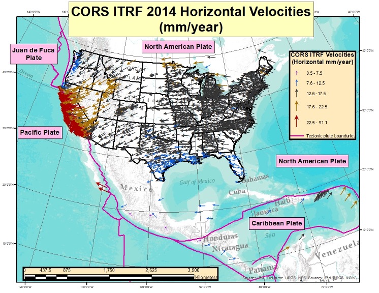
The box titled “CORS ITRF 2014 Horizontal Velocities” provides the horizontal vectors based on NGS’s file downloaded on Jan.13. Only CORSs designated as operational and computed velocities were included in the plot.
I have also created a table that includes a summary of the ITRF rates for CORS labeled as part of the United States. The table includes the following information for each State and Territory of the United States:
- Number of CORS
- Minimum Horizontal Velocity (mm/year)
- Maximum Horizontal Velocity (mm/year)
- Average Horizontal Velocity (mm/year)
- Minimum Upward Velocity (mm/year
- Maximum Upward Velocity (mm/year),
- Average Upward Velocity (mm/year).
See the table below.
Table of ITRF 2014 Horizontal and Upward Velocities of U.S. CORSs
Computed Velocities Only (Downloaded Jan. 13, 2022)
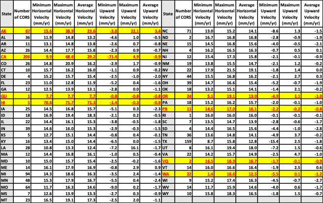
The highlighted territories in the table are not on the North American plate (GU, HI, PR and VQ), and the highlighted states are partly inside or close to the boundary of the North American plate (CA, OR, WA). This is one of the reasons why their minimum and maximum horizontal velocity values are different from most of the other states’ values.
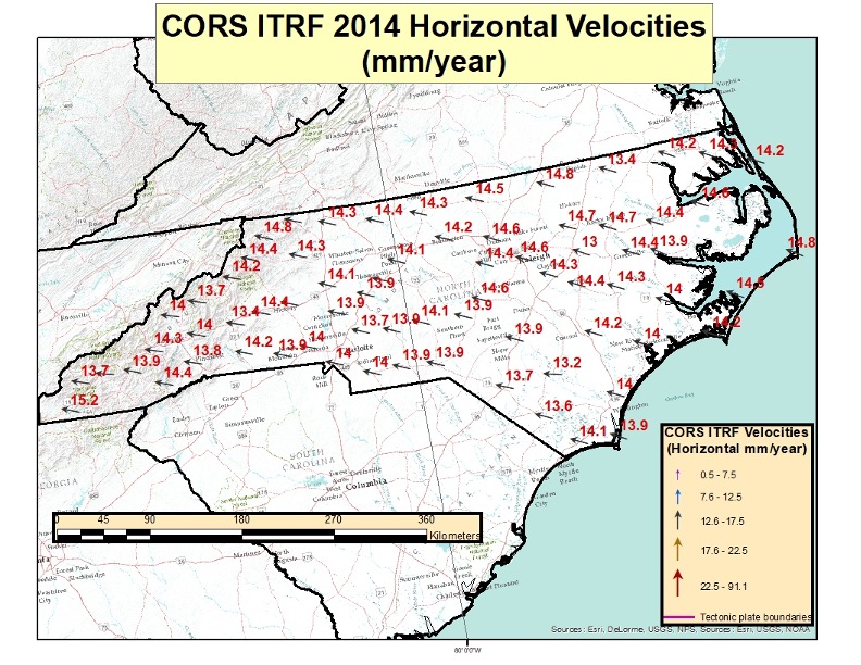
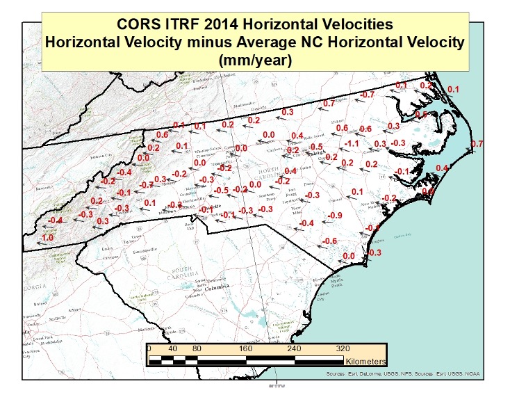
To visualize the relative differences in horizontal velocities between neighboring CORSs, I plotted the ITRF 2014 Horizontal Velocities for CORSs located in North Carolina (see the box titled “CORS ITRF 2014 Horizontal Velocities in North Carolina”). Looking at the figure, it’s obvious that all of the velocities are around 14 mm/year and moving in the same direction.
CORS ITRF 2014 Horizontal Velocities in North Carolina
Computed Velocities Only (Downloaded Jan. 13, 2022)
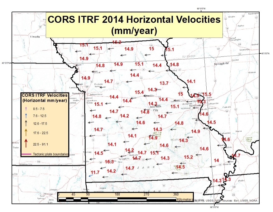
I plotted the horizontal velocities for Missouri to provide an example of the velocities in the central region of the conterminous United States. The magnitude of the velocities is similar to that for North Carolina, but the direction of the vector is slightly different. North Carolina’s average horizontal velocity is 14.1 mm/year and Missouri’s average horizontal velocity is 14.6 mm/year.
CORS ITRF 2014 Horizontal Velocities in Missouri
Computed Velocities Only (Downloaded Jan. 13, 2022)
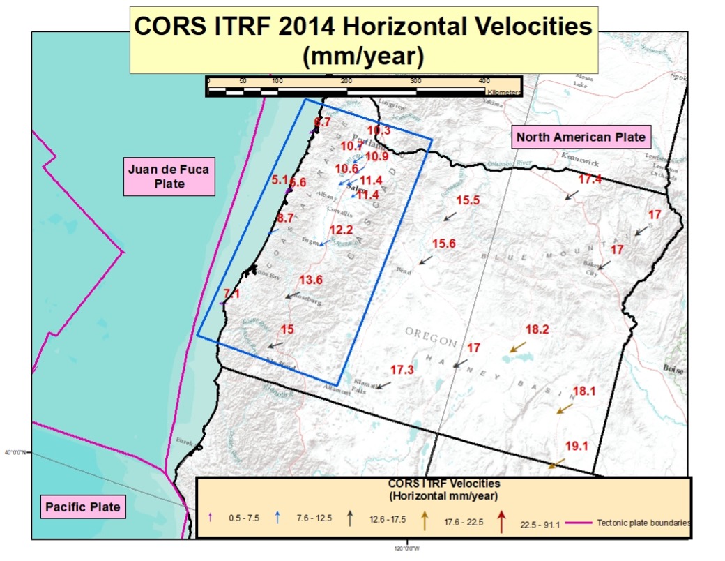
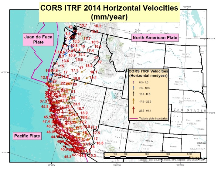
To emphasize the differences along the boundaries of the tectonic plates, I’ve included a plot of the CORS ITRF 2014 horizontal velocities for the State of Oregon and a plot of the states along the West Coast of the United States. See the boxes titled “CORS ITRF 2014 Horizontal Velocities in Oregon” and “CORS ITRF 2014 Horizontal Velocities Along West Coast of CONUS.” As indicated in the plot, there are significant changes in horizontal velocities near the Oregon coast. The values decreased by about 10 mm/year from the inland CORS to the CORS along the coast.
CORS ITRF 2014 Horizontal Velocities in Oregon
Computed Velocities Only (Downloaded Jan. 13, 2022)
The plot of the CORS ITRF 2014 Horizontal Velocities Along West Coast of CONUS clearly indicates the change in magnitude the closer the CORS are to the Pacific and Juan de Fuca plates.
CORS ITRF 2014 Horizontal Velocities Along West Coast of CONUS
Computed Velocities Only (Downloaded Jan. 13, 2022)
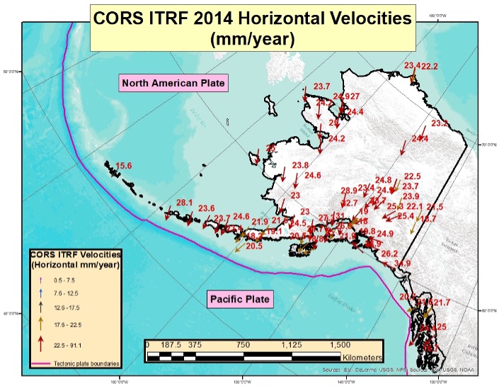
For completeness, I’ve also included a plot of the horizontal velocities for Alaska.
CORS ITRF 2014 Horizontal Velocities in Alaska
Computed Velocities Only (Downloaded Jan. 13, 2022)
To better visualize the horizontal and upward velocities of CORS among states, I plotted the average horizontal and upward velocity value for each state based on that states’ CORS. See the box titled “Average Velocities by State.”
Average Velocities by State
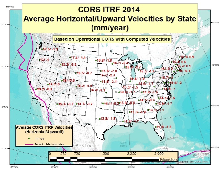
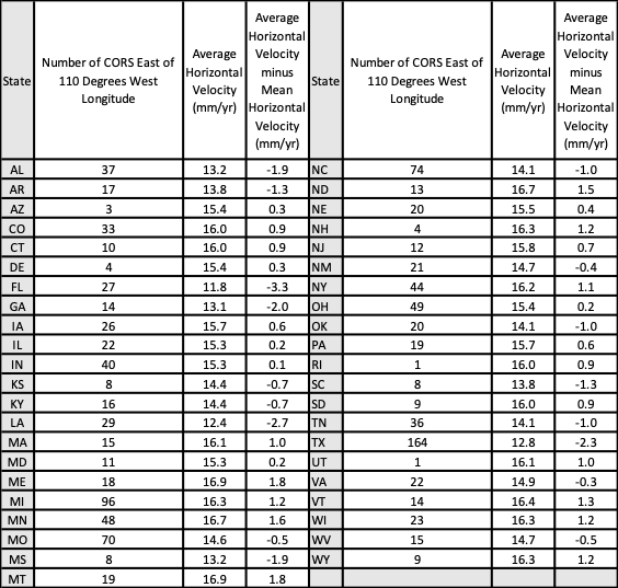
I also computed an average horizontal velocity value based on CONUS CORS east of 110° west longitude (denoted here as a regional horizontal velocity value). [I used the CORSs east of 110° west longitude to be consistent with NGS’s Figure 2 in NOS NGS 62.]
The box below summarizes the average horizontal motion for each state. The table provides:
- The Number of CORS East of 110° West Longitude
- Average Horizontal Velocity (mm/year)
- Average Horizontal Velocity minus Regional Horizontal Velocity (mm/year).
This provides an estimate of the variation of the relative horizontal motion between States.
Table of ITRF 2014 Horizontal Velocities minus Regional Velocity of U.S. CORS East of 110° West Longitude
The box titled “Horizontal Velocities in NC Minus Average Velocity” depicts the resulting horizontal velocities with an average velocity removed (the average velocity was based on NC CORS only) for all CORS in North Carolina. As one can see from the plot, most of the resulting horizontal velocities are less than 1 mm/year, but they are still not zero. Once again, this is only meant to provide an idea of the size of the relative vectors between CORS in North Carolina.
As indicated in the NOS NGS 62 report, these horizontal velocities will be small, but they will not be zero. Hence the reason that NGS needs to provide models and tools for users to be able to transform coordinates between the four national frames (NATRF, PATRF, CATRF and MATRF) and the International Terrestrial Reference Frame (ITRF), as well as to estimate coordinates at epochs different from the survey observation epoch by accounting for movement within the reference frame. Surveyors in California have been dealing with these types of movements for many years now.
Horizontal Velocities in NC Minus Average Velocity
(Downloaded Jan. 13, 2022)
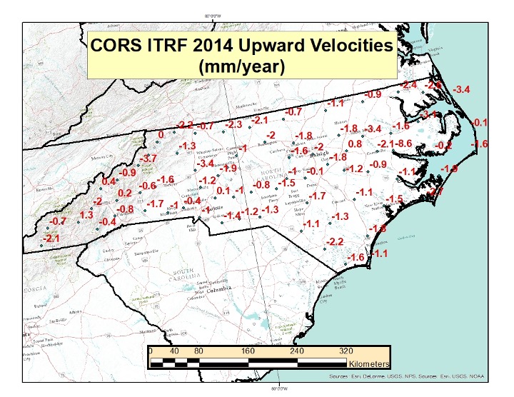
I plotted the ITRF 2014 upward velocity values of the CORS in North Carolina to depict an estimate of the vertical movement of the CORS in North Carolina. See the box below. The vertical velocities values are much less than the horizontal velocities, but they still are not zero. A future column will address the upward velocities based on the ITRF 2014 rates and crustal movement models.
CORS ITRF 2014 Upward Velocities in North Carolina
(Downloaded Jan. 13, 2022)
This column explained why it is important to account for movement of marks everywhere and not just in areas influenced by active crustal movement due to earthquakes such as in Southern California. It provided information about the CORS rates of movement based on NGS’s ITRF2014 coordinates and velocity information. It highlighted NGS’s reports that describe models that will facilitate users transferring coordinates between reference frames and dealing with intra-frame movement between marks based on survey performed at different epochs. This is not just a horizontal positioning issue.
A future column will address estimates of vertical velocities in the new, modernized NSRS.