A “GNSS radial survey” is a surveying technique where a central control mark is established within an area, and vectors are measured from the central control mark to various other marks of interest surrounding the central control mark, essentially creating a “spoke-like” network design.
Plot of OPUS Projects network diagram. Hub is Addicks CORS, all marks are simultaneously observed during the session. (Photo: Dave Zilkoski)
Why not use a GNSS radial survey when establishing geodetic control networks?
Basically, you cannot directly calculate a “relative accuracy” between two marks if no observations are taken between them. That said, a direct measurement such as a GNSS vector allows error propagation between two marks. Therefore, using the “spoke-like” concept, you know the relative accuracy between the central control mark and a single mark at the end of a single spoke. Still, you don’t know the relative accuracy between marks on the different spokes.
Anyone who has used OPUS Projects or seen presentations on OPUS would think, based on the OPUS Project’s HUB processing strategy, that OPUS Projects was performing a radial survey.
When using OPUS Projects, NGS recommends that users select one CORS as a HUB while processing GNSS session data. In the example here, the Addicks CORS (ADKS) was used as the HUB in data processing. So, why is this not considered a radial survey? It may look like a GNSS radial survey but there’s a lot that goes on behind the scenes.
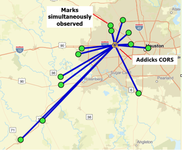
The bottom line is that OPUS Projects is denoted as a simultaneous (session) processor. This means the vector solution is computed from simultaneous processing of all independent vectors with mathematical correlations between all simultaneously observed vectors. OPUS Projects processing includes all independent vectors along with mathematical correlations to provide the relative connection to marks that are simultaneously observed. In the example above, when processed by OPUS Projects, all the marks occupied (indicated by the lines connecting to the Addicks CORS HUB) will have correlations computed between each other. These correlations are included in the data that is used in the least squares adjustments that are performed during the OPUS Projects workflow (NGS uses a file denoted as the gfile to document the correlations.)
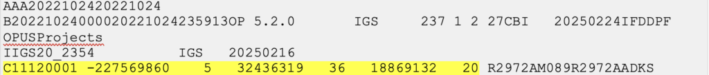
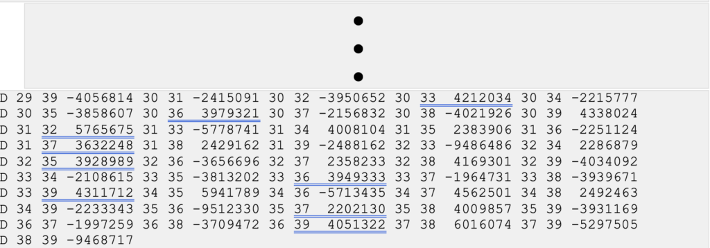
The image below provides a sample of mathematical correlations between marks simultaneously observed during the session. The gfile can be a large file when the survey includes a lot of simultaneously observed marks because there will be correlations between all marks. There were 13 marks simultaneously observed during the sample session, so the “spoke-like” diagram includes imaginary lines between every mark because of the mathematical correlations between these marks.
Excerpt from an output from simultaneous (session) processing. (Gfile contains baseline information with mathematical correlations.)
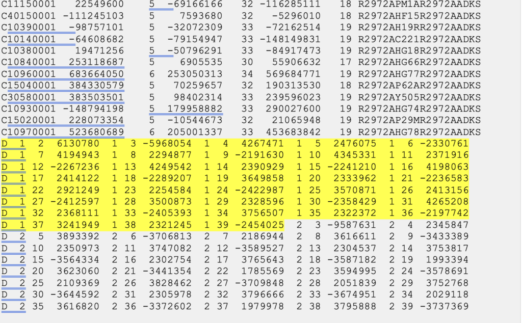
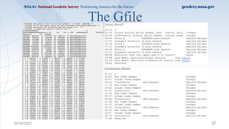
Dan’s presentation included a slide that described the file’s format. The file provides information on the vectors (delta X, delta Y, delta Z and their standard deviations) between the HUB and the individual marks, plus the mathematical correlations between all marks simultaneously observed during the session. I have highlighted a vector’s components and standard deviations and a set of mathematical correlations.
The image below, from Dan’s presentations, describes the format of NGS’s gfile.
Photo: NGS
Some software programs perform what is called sequential (baseline) processing, which involves processing one vector at a time and ignoring the mathematical correlation between baselines observed in the same session. So, what does this mean, and why is it important?
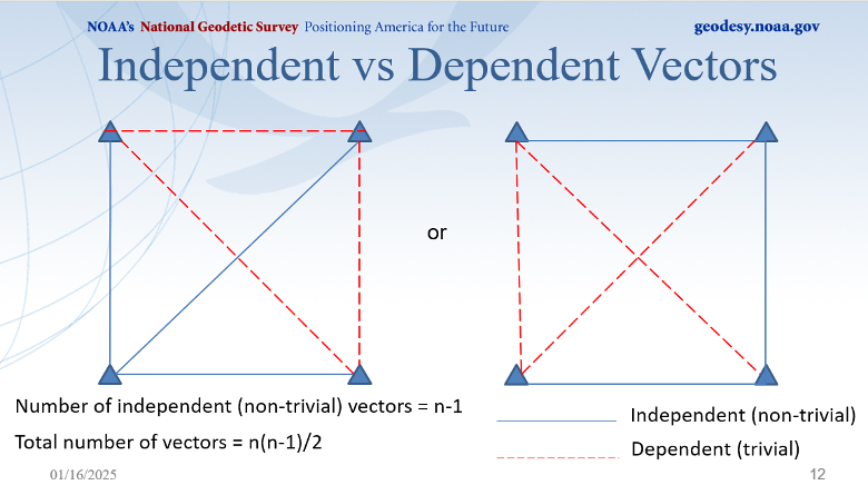
A couple of definitions are necessary to understand the concept. Independent baselines are baselines where no other baseline is a linear combination of another baseline. Linearly dependent (trivial) baselines are baselines that are linear combinations of another baseline. Basically, once you have used a particular set of data to compute a vector, you can’t use the same data to compute a different vector.
Dan did a nice job during his webinar explaining what baselines are considered trivial and what baselines are non-trivial. This is very important because if your software is a sequential (baseline) processor, you must ensure that trivial vectors are not included with the non-trivial vectors. As Dan highlights in his webinar, dependent vectors are not additional observations. But they do offer useful information if treated properly.
Photo: NGS
There was a 1992 study performed by Michael Craymer and Norm Beck, “Session Versus Baseline GPS Processing,” that explained the differences between sequential baseline processing and simultaneous (session) processing, and what the user needed to do to use sequential baseline processing. Basically, when all the trivial vectors are added to the adjustment, they are treated like additional independent observations, resulting in an inflating degree of freedom and overly optimistic error estimates. If all possible vectors are processed, then resulting coordinates may essentially be the same as in simultaneous (session) processing, but statistics will be overly optimistic and misleading. The 1992 paper does state that the two different processing techniques can produce the same results.
“It is shown that using all possible baseline solutions (with the covariance matrix scaled by n/2, where n is the number of simultaneously observing receivers) is mathematically equivalent to session processing with all correlations only under certain conditions. This equivalence is verified empirically using simulated and real data. However, the conditions under which this equivalence holds are difficult to achieve in practice.”
Users who process data using a sequential processor should read the 1992 study by Craymer and Beck to understand the conditions under which the two processes generate the same results.
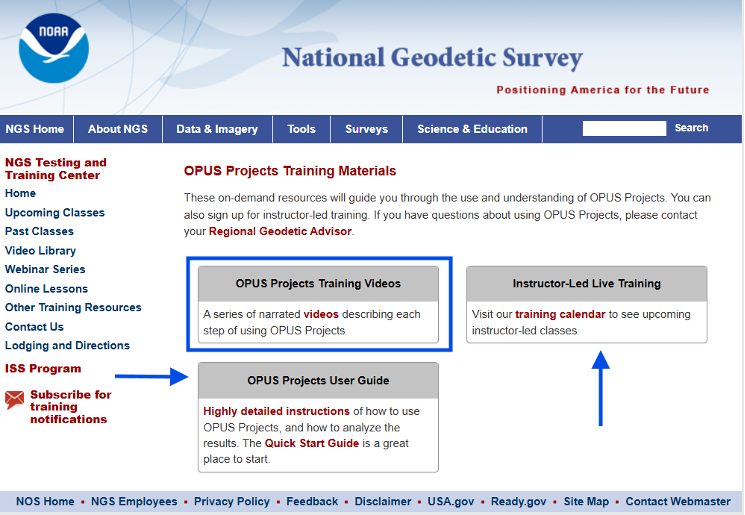
I would encourage all individuals that process GNSS data, regardless of which software you use, to download the NGS OPUS User Forum webinar. NGS also has a website that provides training material on the use of OPUS Projects. The more you know about the software you use, the better you will be prepared to address issues associated with your survey results.
NV5 Geospatial, a large geospatial data company, provides services for airport projects across the United States and U.S. territories — mainly supporting airport planning and engineering firms that must meet FAA survey and mapping requirements for data collection at airports. “We generally are a sub-consultant to them, helping them achieve those survey standards for collecting the data and submitting it to the FAA,” said David Grigg, the company’s Aviation Program Director. Typically, this is around planning projects such as airport layout plans and master plans, but also engineering projects such as runway extensions and runway reconstructions.
As an example, Grigg cited the extension of a runway, which requires new flight procedures to be established. “Two survey missions are required for runway extensions. The primary mission is to establish control for the aerial imagery. Using the imagery, control and design data, we check for obstacles photogrammetrically. That data is sent to the FAA and procedures are developed. After construction is complete, we go back to the airport to survey the changed runway and navigational aids (NAVAIDS) to verify that what was designed was ultimately built.”
Another way in which NV5 Geospatial supports airport clients is by conducting obstruction studies around them for vegetation management. “That’s generally where we pull in the lidar surveys,” said Grigg. The FAA’s standards for relative and absolute positioning accuracy for trees are “rather generous” by surveying standards, he said. “We’re talking two to three feet vertically and twenty feet horizontally. It’s not like a typical mapping job where you’re guaranteeing it to one foot or better horizontally and half foot or better vertically.”
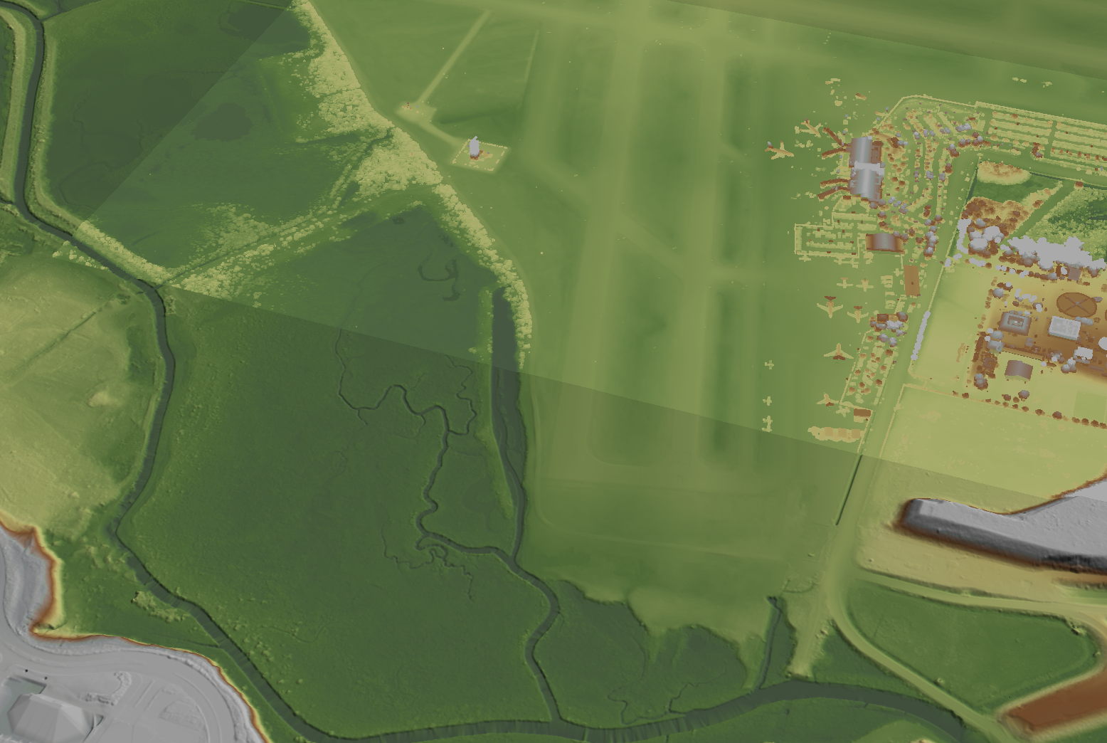
The FAA, he points out, has published guidance on how lidar may be used. “We mostly use aerial photogrammetry to support projects in the FAA’s airports GIS program. When we collect lidar at an airport, we do it to generate contours and to identify individual tree canopies. Our lidar-derived data is most often developed to benefit airports for tree mitigation not for FAA airports GIS survey projects.”
Image: NV5 Geospatial
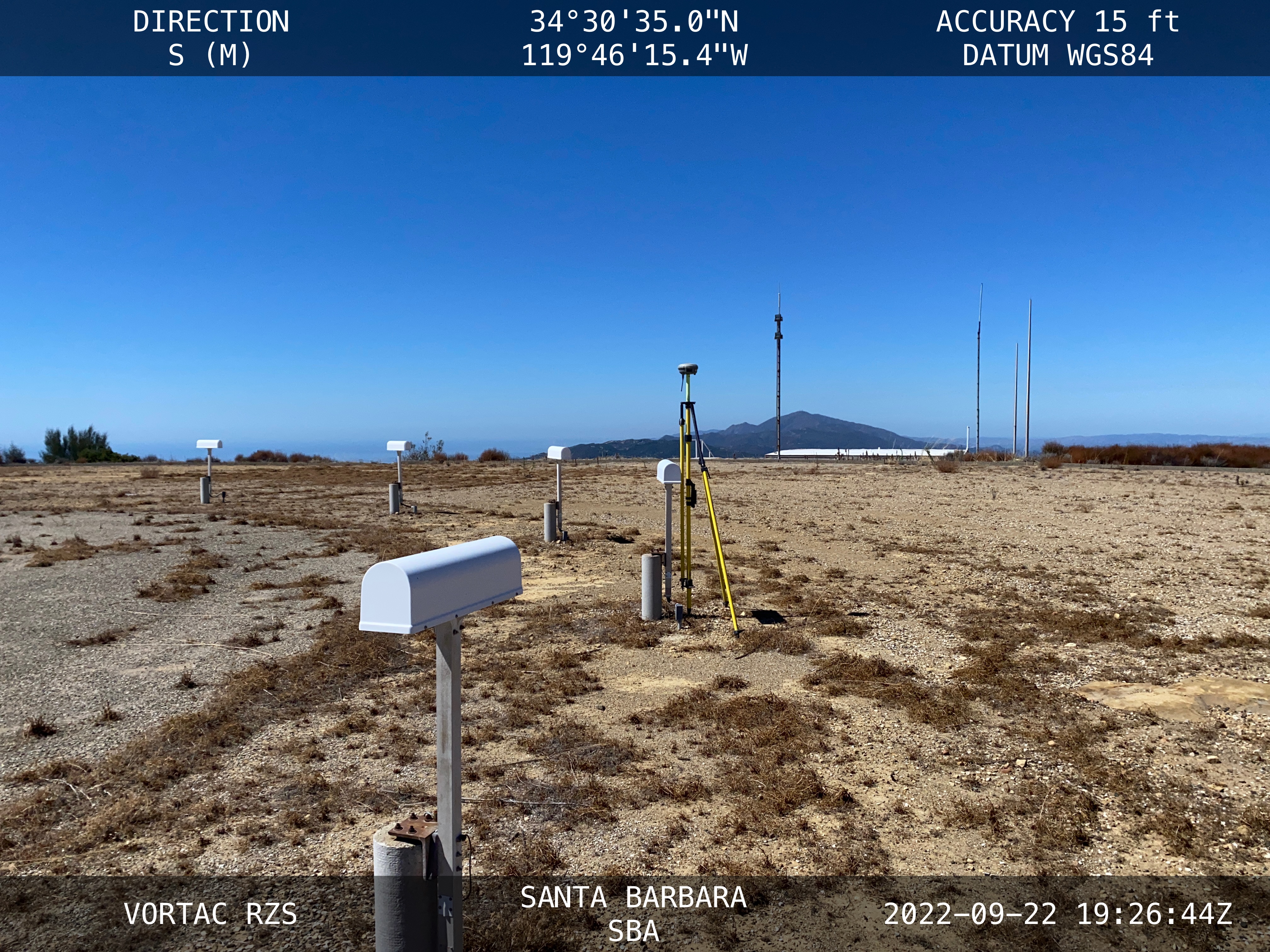
On the other hand, the FAA has strict requirements regarding metadata to document when, where, and how each control point is collected. “At the time of the survey, photographs are taken of the GPS units from different angles and cardinal directions,” Grigg said. “This is visual documentation for NGS that the surveyed point is at the location described. ”
Another challenge for surveyors working at airports is that they are required to pull back for incoming aircraft. “Obviously, you will have some logistical issues at busy airports,” said Grigg. Surveyors are required to have special lights and markings on any vehicles that enter the airport property to ensure ground and air visibility. Aircraft movement also impacts surveyors as they must move away from the runway safety area (RSA) for take-offs and landings. Busier airports are surveyed at night, when air traffic is reduced or runways are closed.
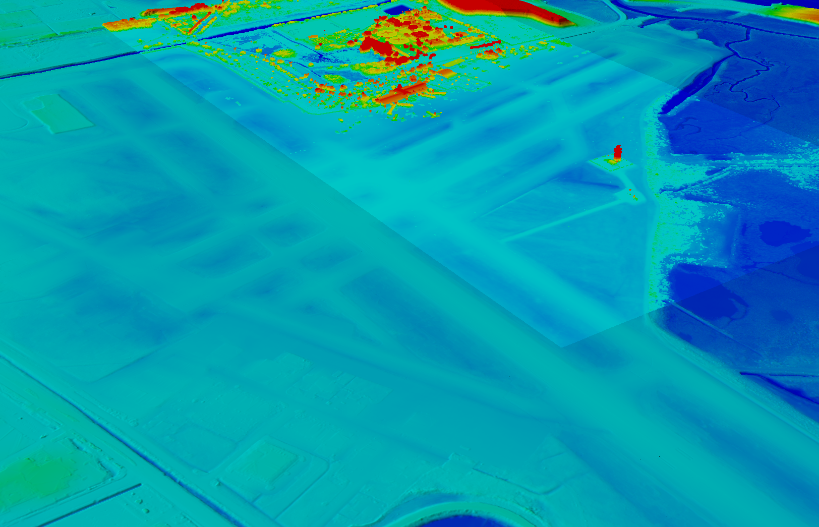
Image: NV5 Geospatial
A typical project for a small airport takes about nine months, while for bigger airports — such as Chicago O’Hare, Dallas-Fort Worth, or Hartsfield-Jackson Atlanta — they can take up to twice as long. “The large hubs update their master plan on a more reoccurring basis, such as every three to five years,” said Doug Fuller, NV5 Geospatial’s Airport Solutions Specialist. “As the airports get smaller, you start stretching out that timeframe.”
Airport survey requirements
[The following was written by NV5 Geospatial and only lightly edited by GPS World.]
Airports have surveys conducted for many different reasons. However, all survey types require the collection, classification and reporting of accurate data about the project. The methodology selected to gather the information is up to the professional surveyor’s judgment. Some features require observation through ground field methods, while others lend themselves to collection via remote sensing technologies.
All surveys start with a search for existing airport control, which are called Primary Airport Control Points (PACS) and Secondary Airport Control Points (SACS). These are points on the airport that have been adjusted by the National Geodetic Survey (NGS). This ensures that the survey is done on the National Spatial Reference System (NSRS).
A typical survey includes surveying the runway, the end points, any displaced thresholds, and a profile along the centerline of the runway. If the centerline marker is not in the correct location or if it is not there at all, the surveyor will make the necessary measurements to establish the proper location and set a new marker. Next the surveyor must locate all NAVAIDS and survey them at the proper location as described in FAA Advisory Circular 150/5300-18B.
After the NAVAIDS are located, the photo control survey will be done. This still requires the PACS and SACS to be the points of origin of the survey. The base requirement as described in FAA Advisory Circular 150/5300-16C is to survey ten photo control points and five check points. The check points are sent to NGS’s Online Positioning User Service (OPUS). This is used to check that the survey was done on the NSRS and that the compilation meets FAA standards.
The standards the surveyor must meet vary depending on the equipment type or photo control point. Examples of the accuracy requirements for the NAVAIDS are as follows:
Point
Horizontal
Vertical
Distance measuring equipment
+/- 1 ft
+/- 1 ft
Glideslope
+/- 1 ft
+/- 0.25 ft
Inner marker
+/- 10 ft
+/- 20 ft
Localizer
+/- 1 ft
+/- 0.25 ft
Runway end point
+/- 1 f ft
+/- 0.25 ft
Runway profile points
+/- 1 f ft
+/- 0.25 ft
Photo control
+/- 1 ft
+/- 1 ft
PACS and SACS
X
Y
Z
Ellip.
Inverse from PACS to SACS
surveyed relative to published
0.09 ft
0.09 ft
0.15 ft
0.13 ft
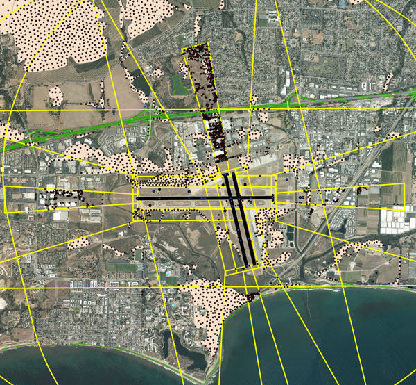
When surveying on airport property, the largest challenge is always accessing the runway safety area to locate the runway ends and profiles. At small airports Surveyors must work when the runway is not busy; at airports with FAA control towers when the runway is closed. Frequently this is done overnight. Other challenges include access to the FAA NAVAIDS. Some of them must be turned off to be surveyed and others require survey points on which it is not possible to set an instrument. When we are not able to occupy a point, we collect it by surveying multiple equidistant locations around the NAVAID and averaging them.
Image: NV5 Geospatial
NV5 Geospatial surveyors use a combination of real-time (R/T) and post-processing techniques. We also use OPUS with the PACS and SACS and the five check points. Once the PACS and SACS have been determined to be stable, the proper coordinates are applied to them and the R/T points are adjusted using Trimble Business Center (TBC). NV5 Geospatial uses Trimble TRM-R8s and we recently added TRM-R12i receivers to our equipment. We use ground control points to orient the photography and to calibrate the lidar.
February’s column focused on potential errors in orthometric heights using a digital barcode leveling system with multi-piece leveling rods. As stated in the column, businesses need to make decisions based on expenses and ultimately on the profit margin; but making a business decision that results in a bad technical outcome is never the right decision. This newsletter column is going to highlight a new feature in the National Geodetic Survey (NGS) Beta OPUS Projects 5.1 routine permitting the use of RTN vectors to support the development of the 2022 Transformation model.
On Jan. 12, NGS held a webinar titled “Using RTN Data in OPUS Projects 5 for GPSonBM.” Users can download the video and PowerPoint slides here.
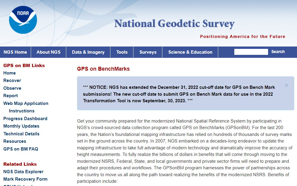
I’ve been highlighting NGS’s GPS on Bench Mark program that supports the 2022 Transformation Tool in my columns since 2018. NGS delayed the completion date for the new modernized NSRS until 2025, so they have extended the cut-off date for submitting GPS on Bench Mark data for use in the 2022 Transformation Tool until Sept. 30.
NGS GPS on BenchMarks Program (Image: NGS website)
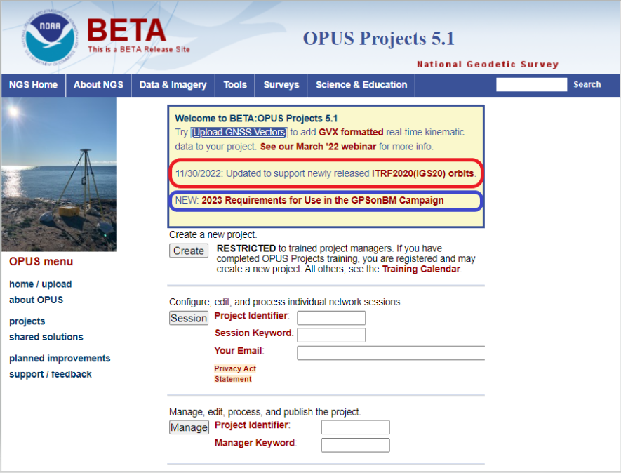
NGS has been developing tools that facilitate submitting data to the NGS GPS on BM campaign such as OPUS Share. The latest tool is the OPUS Project 5.1 routine that allows the use of RTN vectors. OPUS Projects 5.1 is a beta product, but NGS is now allowing users to use the routine to submit data for the GPS on BM campaign. My October 2021 column highlighted NGS’s Beta OPUS Projects 5.1.
The 2023 requirements for using OPUS Projects in the GPS on BM program (Image: NGS website)
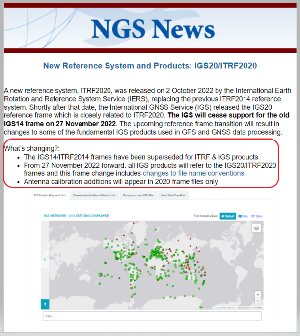
I’d like to note that OPUS has been updated to support the newly released ITRF2020 (IGS20) orbits. My October 2022column discussed the latest International Terrestrial Reference Frame of 2020 (ITRF2020) released by the International Earth Rotation and Reference System Service (IERS). A previous NGS news bulletin provided a statement about the new reference system and products.
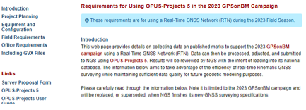
Clicking on the link titled “NEW: 2023 Requirements for Use in the GPSonBM Campaign” on the OPUS Projects 5.1 webpage provides the requirements for using OPUS Projects 5.1 and Real-Time Network (RTN) data to support the 2022 Transformation Tool; that is the 2023 GPS on BM campaign. There are five sections in the writeup: Introduction, Project Planning, Equipment and Configuration, Field Requirements and Office Requirements. The Introduction section states that the requirements are limited to the GPS on BM Campaign and will be replaced, or superseded, when NGS finishes its new GNSS surveying specifications.
Introduction Section from Requirement Write Up (Image: NGS website)
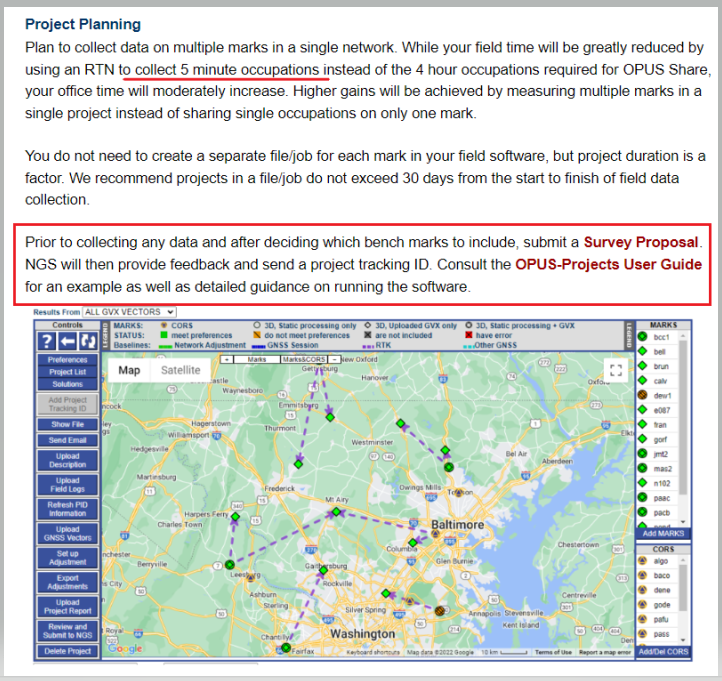
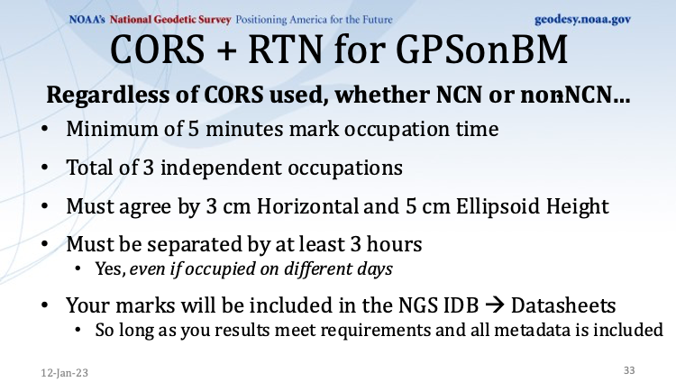
The project planning section of the announcement states that RTN vectors of 5-minute occupations can be used instead of the 4-hour occupations required for OPUS Share.
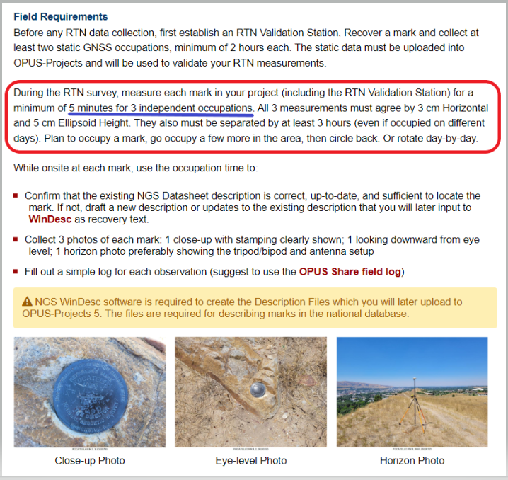
However, the Field Requirement section states that the mark must be occupied three different times.
“During the RTN survey, measure each mark in your project (including the RTN Validation Station) for a minimum of 5 minutes for three independent occupations. All three measurements must agree by 3 cm horizontal and 5 cm ellipsoid height. They also must be separated by at least 3 hours (even if occupied on different days). Plan to occupy a mark, go occupy a few more in the area, then circle back. Or rotate day-by-day,” the section states.
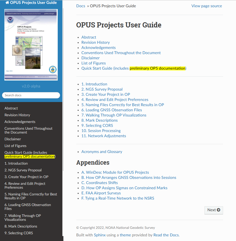
As stated in the section on office requirements for using OPUS-Projects 5 in the 2023 GPS on BM Campaign writeup,“The OPUS-Projects User Guide provides instructions on how to run the software and submit a project to NGS. The User Guide states to follow the steps in the order listed below, and it explains steps 1 – 7 and 9 – 11 in detail. For step 8 and when including GVX data in OPUS-Projects 5, refer to those portions of the User Guide’s Quick Start which are highlighted in yellow. NGS is working on fully updating the User Guide to include more details; for now, use the Quick Start Guide for assistance with GVX.”
I recently used OPUS Projects to analyze some GNSS results using Harris-Galveston Subsidence District CORS and PAMS GNSS data. I want to emphasize that it may seem like a lot of work the first time you use the routine, but NGS makes it fairly simple to complete each task. The manual is very complete and does a good job of describing every step. The manual can be downloaded here. In my experience, the most time-consuming task is creating the descriptions. There are several items that must be correctly entered because the answer to some entries affect the answers to other entries. That said, NGS supports a description entry software called WinDesc that facilitates entering the appropriate information. The OPUS Projects User Guide provides an appendix that describes using the WinDesc module to enter description metadata.
For marks that are in the NGS database, known as the NGS Integrated Data Base (NGSIDB), WinDesc will import information from NGSIDB, thereby decreasing the number of entries users need to address. In other words, if the mark has a PID then it should be in the NGSIDB. If you are occupying a mark that is part of NGS GPS on Bench Marks website then it probably has a PID and a description in NGSIDB.
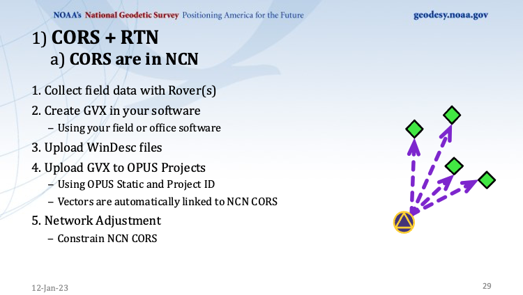
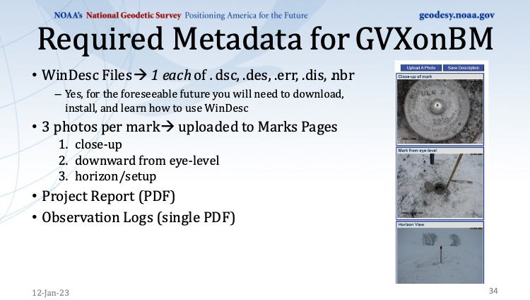
I’ve included three slides from the Jan. 12 webinar that summarize the basic requirements.
This slide is a depiction of how a CORS station must be connected to the RTN vectors. (Image: NGS website)
This slide provides the occupation and precision requirements. (Image: NGS website)
This slide provides a list of the required metadata for the project. (Image: NGS website)
As for the requirement of at least three independent RTN occupations on different times, in my opinion at least one occupation should be on a different day. My October 2021 column addressed a study that reported on using RTN solutions to estimate accurate horizontal and vertical coordinates.
The report stated, “When differenced with coordinates from a static GNSS survey campaign, the horizontal and vertical RMSE of the NRTK-derived coordinates was 2.3 cm horizontally and 4.5 cm vertically at 95% confidence. Repetitive NRTK vectors on each baseline differed between ± 2.4 cm horizontally and ± 3.4 cm vertically at 95% confidence.”
The report also stated, “Adjustment of hybrid survey networks with four repeat NRTK vectors per bench mark produced network accuracies at 95% confidence for the adjusted coordinates at all bench marks less than 1 cm horizontally and 2 cm vertically (ellipsoid height).”
The requirements are limited to the GPS on BM Campaign and will be replaced, or superseded, when NGS finishes its new GNSS surveying specifications.
(Image: Screenshot of Accuracy of GNSS Observation from Tree Real-Time Networks in Maryland, USA)
The paper by Gillins, et. al was presented at the 2019 FIG Working Week held in Hanoi, Vietnam, on April 22–26, 2019. The International Federation of Surveyors (FIG), involves a wide range of professional fields within the international surveying community; this includes surveying, cadastre, valuation, mapping, geodesy, hydrography, and geospatial and provides an international forum for discussion and development to promote professional practice and standards. FIG meetings are held all over the world. I’d like to highlight that the 2023 FIG Working Week is going to be held in Orlando, Florida, on May 28 – June 1, 2023.
NGS will be presenting a full-day worth of content on NSRS Modernization during the FIG Working Week 2023. For the first time in more than 20 years, this annual FIG gathering will take place in the United States, hosted by the National Society of Professional Surveyors (NSPS).
I’ve participated in several FIG meetings. I’ve learned a lot from presentations as well as holding hallway meetings with experts from the international surveying and mapping community. All geospatial users should plan on attending this event. I have provided information about the FIG commissions in my August 2021 newsletter. I would encourage everyone to visit the FIG website and review the information about the 2023 FIG Working Week. The a list of the FIG Commissions can be found here. More information can be obtained on each commission by clicking on its title.
Future columns will highlight the FIG Working Week as the agenda is developed. I would encourage everyone to check NGS’s Website for updates on Beta products and new surveying specifications. Geospatial users should also subscribe to NGS’s News Services at the following here. Check out the NGS News Services site for what’s available.
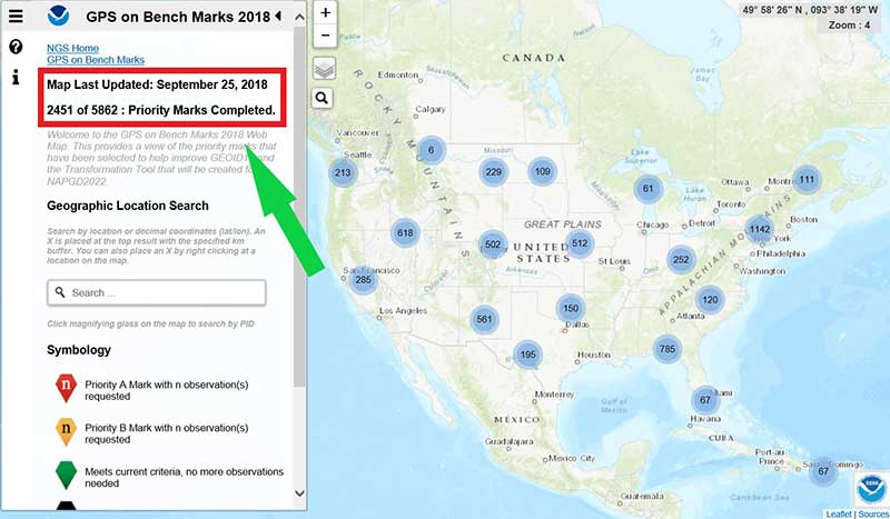
The number of GPS on Bench Mark (BM) stations highlighted as complete on the National Geodetic Survey (NGS) GPS tracking page as of Sept. 25 represents 43 percent of the total number of stations that need to be observed (2451 of 5862 Priority Marks Completed).
These new GPS on BMs observations will be helpful in identifying invalid GPS on BM stations that may have been used in the next hybrid geoid model.
Now that the 2018 GPS on BM program has officially ended for data included in the hybrid model GEOID18, NGS’ GPS on Bench Mark Program will soon be expanded to include other regions and will focus on data to improve NGS datum transformation tools.
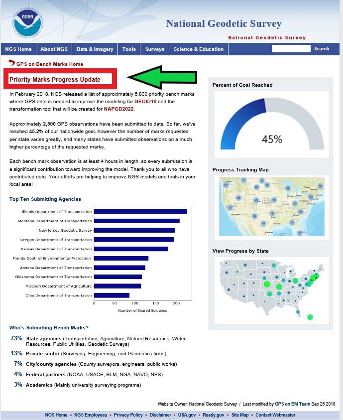
NGS has aided users that are submitting data using OPUS through their GPS on BM website service. Previous columns have highlighted the website. This column will highlight a new feature on the NGS GPS on BMs webpage that displays the progress of priority marks and its associated statistics. This webpage can be accessed through a link on the GPS on BMs Program main webpage — (see highlighted section in box tilted “GPS on BM Project Webpage”). The new webpage provides statistics by state as well as which agencies are submitting the most GPS on BMs data (see the box titled “NGS Webpage of Priority Marks Progress Update”).
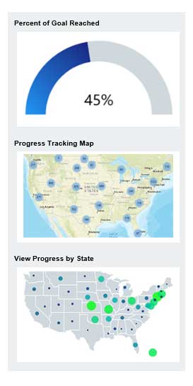
The right side of the webpage provides the percent of the goal reached, a link to the progress tracking map, and a link to progress by state (see box below). The first thing to notice that it provides a current percent of goal reached to date. In this example, the GPS on BM program is at 45 percent complete.
Right Side of Priority Marks Progress Update Webpage
Clicking on the “Progress Tracking Map” picture will bring up the latest map update (see box below). As depicted in the box, as of Sept.25, 2,451 of 5,862 priority marks have been completed. The “Progress Tracking Map” provides information based on the last time the map was updated, and the “Percent of Goal Reached” is based on the most current OPUS Shared solutions submitted. NGS is working toward generating the map and solutions in near real time.
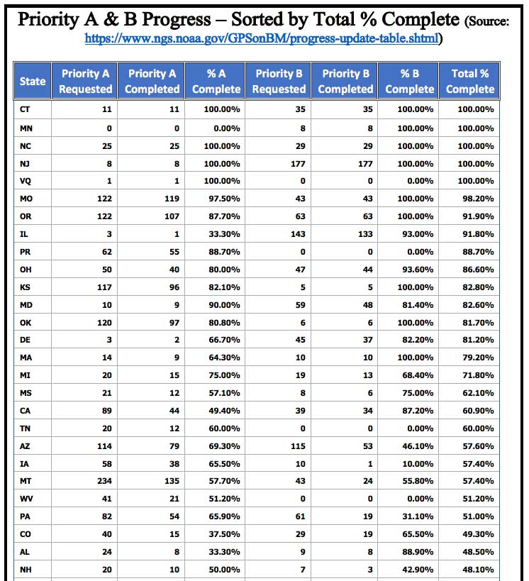
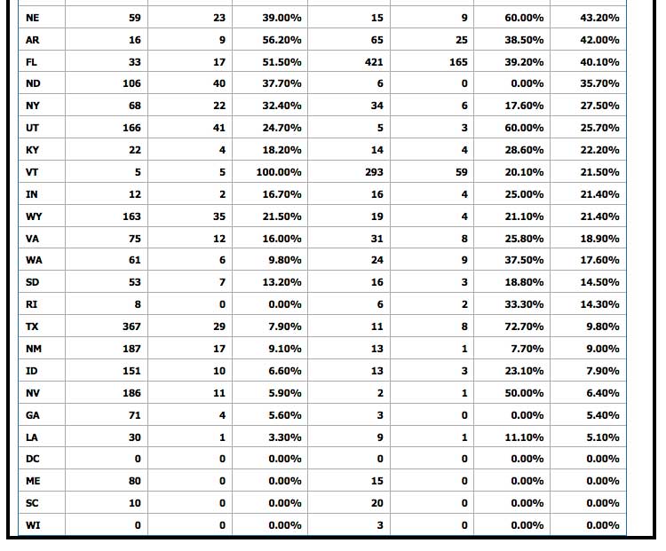
Clicking on the “View Progress by State” picture will bring up a table of progress of priority marks by state (see box titled “View by State Webpage”). As depicted in the box, the following statistics are provided for every state:
Source: National Oceanic and Atmospheric Administration
Source: National Oceanic and Atmospheric Administration
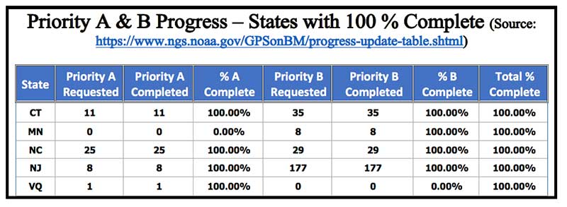
The following states have officially completed 100 percent of their priority A and B stations: Connecticut, Minnesota, North Carolina, New Jersey and U.S. Virgin Islands. Congratulations to these states (see the box titled “Priority A & B Progress – states with 100 percent complete”).
Priority A & B Progress — States with 100 percent complete
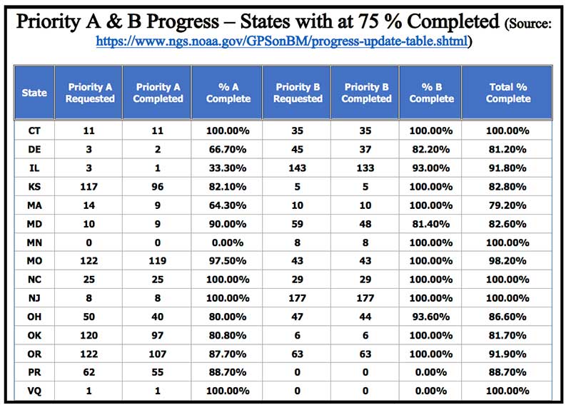
It should also be noted that there are 15 states that have completed at least 75 percent of their priority A and B stations (see box below). This is a tremendous amount of work, and everyone should be commended for participating in the GPS on BM program.
Priority A & B Progress – States with at 75 percent Completed
Source: National Oceanic and Atmospheric Administration
The left side of the webpage provides information on the top submitting agencies. As indicated in the box below, the Illinois Department of Transportation (DOT) and Montana DOT are the two top leaders in submitting GPS on BMs data. They have submitted well over 200 OPUS Shared solutions. The New Jersey and Oregon DOTs are close behind, providing about 200 OPUS Shared solutions.
Left Side of Priority Marks Progress Update Webpage
Source: National Oceanic and Atmospheric Administration
It’s not surprising to see that state agencies have provided the most submissions to the GPS on BM project (73 percent). It’s very encouraging to see that the private sector has provided 13 percent. Having an accurate and reliable hybrid geoid model will assist surveyors in performing their jobs as well as improve their efficiency in performing geodetic surveys requiring heights.
This column provided an update and status report on stations observed in support of the 2018 GPS on BMs program, and highlighting a new NGS GPS on BMs webpage that displays the progress of priority marks and its associated statistics. The number of GPS on Bench Mark stations completed as of Oct. 1 represents 45 percent of the total number of stations that need to be observed.
As I have explained in previous columns, there were many stations with invalid heights that could be used in the next hybrid geoid model unless more bench marks with valid NAVD 88 heights were observed with GNSS.
Many stations with potential invalid published orthometric heights have been identified by the GPS on BM program. This information will be very useful to the surveying and mapping community as well as to NGS.
NGS’ official date for accepted data for inclusion in the next hybrid geoid model, GEOID18, was Sept. 21. However, any OPUS Shared observations submitted before the final version of GEOID18 has a possibility of being included in the model. Even if it’s not included in the hybrid model, it will be very useful for evaluating the reliability of the model.
After the hybrid geoid model, GEOID18, is published, NGS’ GPS on Bench Mark Program will expand to include other regions and will focus on data to improve NGS datum transformation tools. I encourage everyone to continue supporting the GPS on BMs program — not only for improving the development of the 2022 transformation tool, but to assist in identifying bench marks in your local area that have invalid published orthometric heights due to movement.
Once NGS publishes the next hybrid geoid model, GEOID18, OPUS results will probably provide an estimate of the NAVD 88 orthometric height computed using GEOID18 similar to what it does now using GEOID12B.
In my opinion, the results of GEOID18 will be better than GEOID12B in most areas of the United States and should be helpful in identifying stations that have moved since they were last leveled. Submitting your results to OPUS Shared will provide a way for others to analyze the results to determine whether a station has an issue that requires attention.
My last two columns (NGS 2018 GPS on BMs program in support of NAPGD2022 — Part 6 and NGS 2018 GPS on BMs program in support of NAPGD2022 — Part 7) described the National Geodetic Survey’s (NGS) GPS on BMs 2018 interactive web map, and provided an update and status report on stations observed in support of the 2018 GPS on BMs Program. This column will provide another update and status report on stations observed in support of the 2018 GPS on BMs program and provide an example of how the OPUS-shared results filled in a void area in West Virginia that will benefit the development of the hybrid geoid model GEOID18. The column will also provide an example of how OPUS Shared results identified a reset station that has an invalid NAVD 88 height, and the importance of having a least two OPUS Shared results to ensure the reliability of the OPUS solutions.
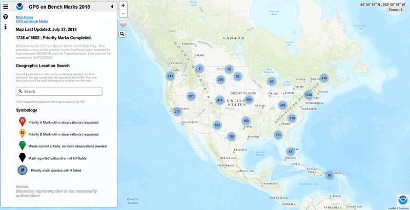
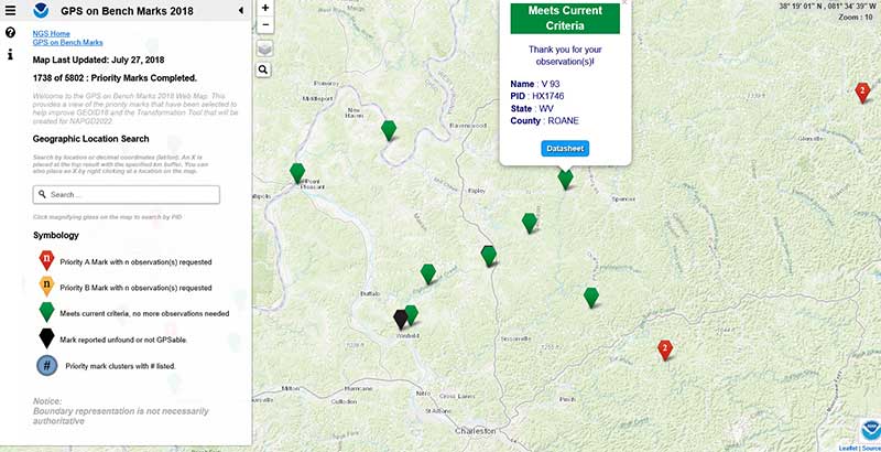
As mentioned in the last column, the GPS on BMs 2018 web page contains a link to a web map where users can determine which bench marks NGS would like users to occupy before the August 31, 2018, deadline. The box titled “2018 Web Map” depicts the map update as of July 27, 2018 (1738 priority marks completed). My last column reported that as of May 29, 2018, there were 1067 priority marks considered completed. During the past two months, 671 more priority stations have been reported completed. This is progress but this still only represents about 30 percent of the priority marks. Hopefully, this will increase dramatically during the month of August. Remember, the cut-off date for data to be included in the creation of the hybrid geoid model GEOID18 is August 31, 2018.
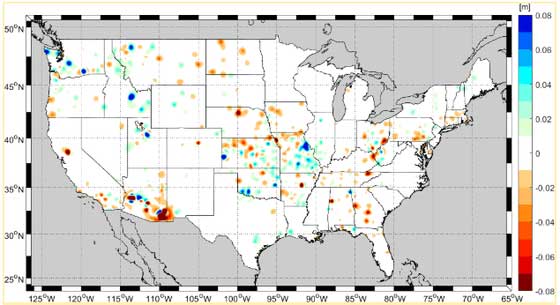
NGS periodically provides an update on the GPS on Bench Marks Program. On July 3, 2018, NGS sent an email to everyone that shared GPS data on NGS bench marks via OPUS or registered for NGS’ February 2018 webinar about GPS on Bench Marks. The email provided an update on the GPS on Bench Marks Program (see box titled “July 3, 2018, NGS Email on GPS on BMs Update”). The map provided in the update indicated that some of the new observations may generate changes between +/- 8 cm.
July 3, 2018, NGS Email on GPS on BMs Update
(Source: Email from National Ocean Service, NOAA; [email protected] to Dave Zilkoski)
Update: GPS on Bench Marks
Over 1,420 marks completed, and two months left to improve GEOID18 accuracy in your area!
Image: National Geodetic SurveyYour observations are making a difference! The color ramp in the map above reflects accuracy improvements in a hybrid geoid model from your recently submitted GPS observations. The improvements will be realized when NGS releases GEOID18.
In case you missed it
In early 2018, NGS released a list of priority bench marks where GPS data is needed to improve GEOID18, NGS’ last planned hybrid geoid model before The North American Vertical Datum of 1988 (NAVD 88) is replaced by the North American-Pacific Datum of 2022 (NAPGD2022). Data to support GEOID18 will be accepted until the end of August 2018. After that, GPS on Bench Marks (GPS on BM) efforts will expand to include other regions and will focus on data to improve future transformation tools.
How can I help?
Following the guidance provided on the NGS GPS on BM website, you can help by collecting static GPS data on adjusted NAVD 88 bench marks and submitting the data to NGS via OPUS Share. To improve efficiency and reduce unnecessary redundancy, we have created a GPS on Bench Marks 2018 web map to help contributors know where we have the data we need and where we still need GPS observations.
Thank you to our contributors
Over 1,700 observations have been submitted to date, completing the required observations for over 1,420 marks from our prioritized list. Each observation requires at least 4 hours of data collection with a survey grade GPS receiver, plus additional time for planning, travel, and data submission, so each one is a significant contribution. Visit the GPS on BM website for updates on our biggest data contributors and each state’s progress toward the goals.
Why are you receiving this email?
• You shared GPS data on NGS bench marks via OPUS, or
• You registered for our February 2018 webinar about GPS on Bench Marks.
We anticipate sending quarterly updates about these and related efforts. If you’d like to opt-out, click the “Manage Subscriptions” at the bottom of this email.
NOAA’s National Geodetic Survey
geodesy.noaa.gov
NGS is tentatively planning another webinar on the GPS on Bench Marks program for August 9, 2018 (2 pm to 3 pm eastern time). NGS will provide an update on the GPS on Bench Mark program and probably will highlight potential improvements between the current hybrid geoid model GEOID12B and the latest prototype version of the future hybrid geoid model GEOID18. I would encourage everyone to sign up for the NGS webinar series.
Source: Plot Generated Using ArcGIS
Users can subscribe to any or all of NGS four public subscription lists — news, webinar, training, and GPS on Bench Marks — by visiting the NGS subscription services web page and submitting their email address for the type(s) of notices they want to receive. (https://www.ngs.noaa.gov/INFO/subscribe.shtml)
As indicated in the figure provided in NGS’ July 3rd update on the GPS on Bench Marks program email, there are many areas of the country that have already benefitted from users participating in NGS’ GPS on BMs program. This column will highlight an area near Charleston, West Virginia, were users have been very active in providing OPUS Shared results. The box titled “GPS on Bench Marks near Charleston, West Virginia” depicts the marks that meet NGS’ criteria and will be involved in the development of the hybrid geoid model GEOID18. As you can see from the plot, there are several new stations that will be used in the development of the model which will help to improve the reliability of the product.
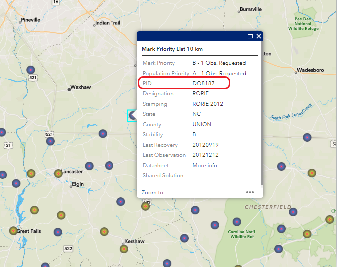
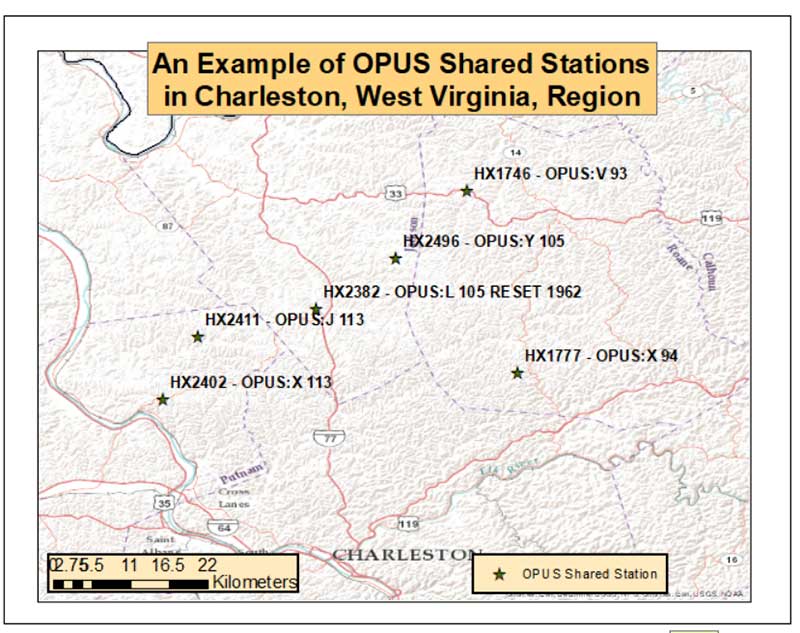
The box titled “An Example of OPUS Shared Stations in Charleston, West Virginia, Region” provides the stations’ PID and OPUS designation. The six OPUS Shared stations cover approximately a 50 km square area. Most of the stations are only 10 km apart. These stations will definitely help to improve the reliability of the hybrid GEOID18 model.
An Example of OPUS Shared Stations in Charleston, West Virginia, region
(Source: Plot Generated Using ArcGIS)
Source: Plot Generated Using ArcGIS
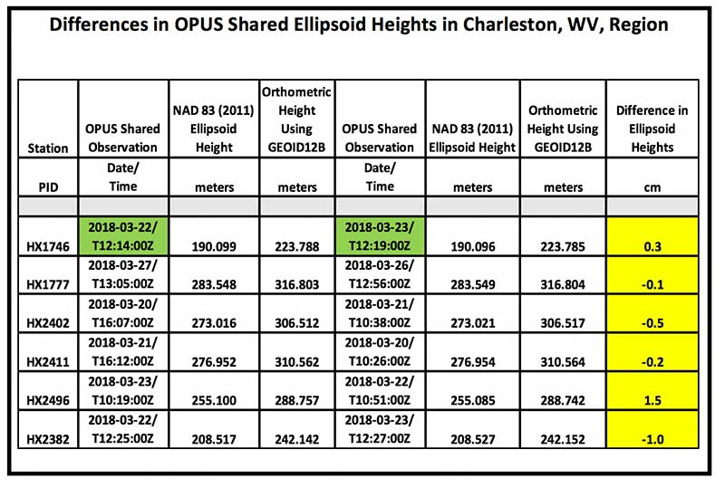
When using OPUS Shared results, users should always check to see if a station has been observed more than once. The box tilted “Differences in OPUS Shared Ellipsoid Heights in Charleston, WV, Region” lists the pairs of OPUS observations for the stations depicted in the previous plot. The column labeled “Difference in Ellipsoid Heights” provides the differences in ellipsoid heights based on the two different OPUS Shared results. All differences are less than 1.5 cm and most are less than 1.0 cm. This is indicating good repeatability to the cm level but this may not be indicating accuracy. These stations were observed one day apart but observed at about the same time of the day. They could have the same systematic errors effecting the results such as multipathing and satellite geometry. When performing the second OPUS Shared observation, users should select a different time of day to improve the chances of detecting, reducing, and/or eliminating the effects of remaining systematic errors.
Differences in OPUS Shared Ellipsoid Heights in Charleston, West Virginia, region
Source: National Geodetic Survey
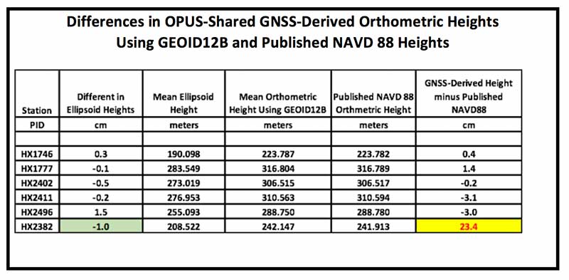
The box titled “Differences in OPUS-Shared GNSS-Derived Orthometric Heights Using GEOID12B and Published NAVD 88 Heights” provides the differences between the GNSS-derived orthometric heights using GEOID12B and the published NAVD 88 values. This table indicates that there is a large difference (23.4 cm) for station HX2382 (L105 Reset 1962). Since the two ellipsoid heights only differ by 1.0 cm, this is an indication that the station probably moved since it was Reset or the reset observations were performed incorrectly. Either way, this station should not be used in the development of the hybrid model or used by anyone for geodetic control.
Differences in OPUS-Shared GNSS-Derived Orthometric Heights using GEOID12B and Published NAVD 88 Heights
Source: National Geodetic Survey
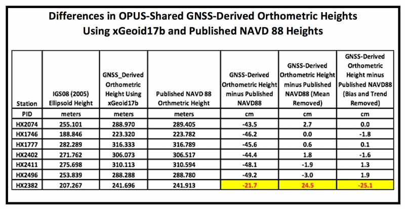
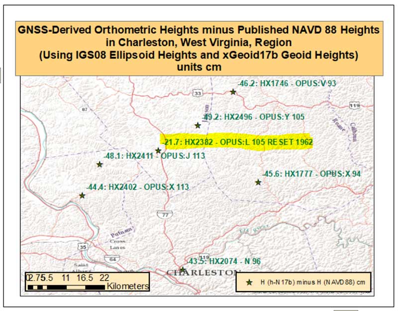
Since GEOID12B is a hybrid geoid model that was designed to be consistent with NAVD 88 values, I always compute differences between GNSS-derived orthometric heights using the experimental geoid model and published NAVD 88 height values. I described this process in my October 2015 column (http://stage.globalpositioningnews.com/establishing-orthometric-heights-using-gnss-part-3/). The box titled “Differences in OPUS-Shared GNSS-Derived Orthometric Heights Using xGeoid17b and Published NAVD 88 Heights” provides the differences between the GNSS-derived orthometric heights estimated using IGS08 (2005) ellipsoid heights with the xGeoid17b geoid model and published NAVD 88 heights. The values in the column labeled “GNSS-Derived Orthometric Height minus Published NAVD 88” represent an approximate difference between NAPGD2022 and NAVD 88. The box titled “OPUS-Shared GNSS-Derived Orthometric Heights Using xGeoid17b minus Published NAVD 88 Heights” provides a plot that depicts these differences.
Differences in OPUS-Shared GNSS-Derived Orthometric Heights Using xGeoid17b and Published NAVD 88 Heights
Source: National Geodetic Survey
OPUS-Shared GNSS-Derived Orthometric Heights Using xGeoid17b minus Published NAVD 88 Heights
(Source: Plot Generated Using ArcGIS)
Source: Plot Generated Using ArcGIS
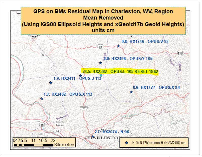
Once again, it should be noted that PID HX2382 value is much different from the other values. To look for outliers, a mean difference was removed from the results. The box titled “OPUS-Shared GNSS-Derived Orthometric Heights Using xGeoid17b minus Published NAVD 88 Heights with a Mean Value Removed” makes it easier to see that station HX2382 is an outlier. The station is approximately 25 cm different from its neighboring stations that are only 10 km away. As previously mentioned, this station apparently moved since being Reset in 1962 or the reset observations were performed incorrectly. Identifying stations that have moved since the last time they have been leveled is one of the benefits of participating in the GPS on BMS program.
OPUS-Shared GNSS-Derived Orthometric Heights Using xGeoid17b minus Published NAVD 88 Heights with a Mean Value Removed
(Source: Plot Generated Using ArcGIS)
Source: Plot Generated Using ArcGIS
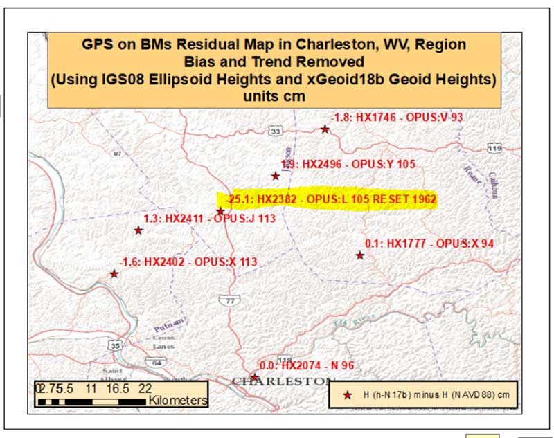
For completeness, both a bias and trend were removed from the differences since IGS08 (2005) GNSS-derived orthometric heights and NAVD 88 heights indicate that there’s an apparent long-wavelength trend between the two sets of values. The box titled “OPUS-Shared GNSS-Derived Orthometric Heights Using xGeoid17b minus Published NAVD 88 Heights with Bias and Trend Removed” depict the differences with a bias and trend removed. As in the other figures, PID HX2382 clearly indicates that it is an outlier relative to its neighbors. This station would be rejected by the geoid team when creating the next hybrid geoid model.
It should be noted that except for the Reset station, all of the differences are less than 2 cm. Although, some relative differences between closely-spaced stations approach 4 cm. For example, the differences between stations HX1746 and HX2496 is -3.7 cm (-1.8 cm – 1.9 cm). The differences in ellipsoid heights from the OPUS Shared solutions are all less than 1.5 cm, even the differences between ellipsoid heights for station HX2382 is only 1 cm. This is an indication that the reset station, HX2382, does not have a valid NAVD 88 published height and should not be used as control. Surveyors that adhere to the FGCS specifications and procedures would realize that this station did not have a valid NAVD 88 height and would not use the published NAVD 88 as control in their project. For example, surveyors performing a leveling project would perform a 2- or 3- mark leveling tie and the results would indicate that the station had moved since it was last leveled.
OPUS-Shared GNSS-Derived Orthometric Heights Using xGeoid17b minus Published NAVD 88 Heights with Bias and Trend Removed
(Source: Plot Generated Using ArcGIS)
Source: Plot Generated Using ArcGIS
This type of validation procedure should also apply for OPUS users. If a user obtains one OPUS solution and proceeds to perform a survey from that station, the user does not know whether the OPUS height value is reliable or accurate. One solution does not provide any indication of reliability.
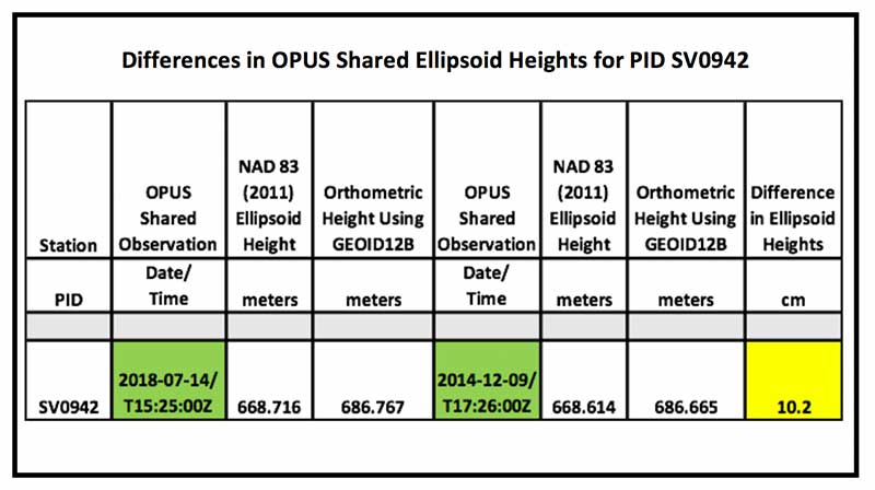
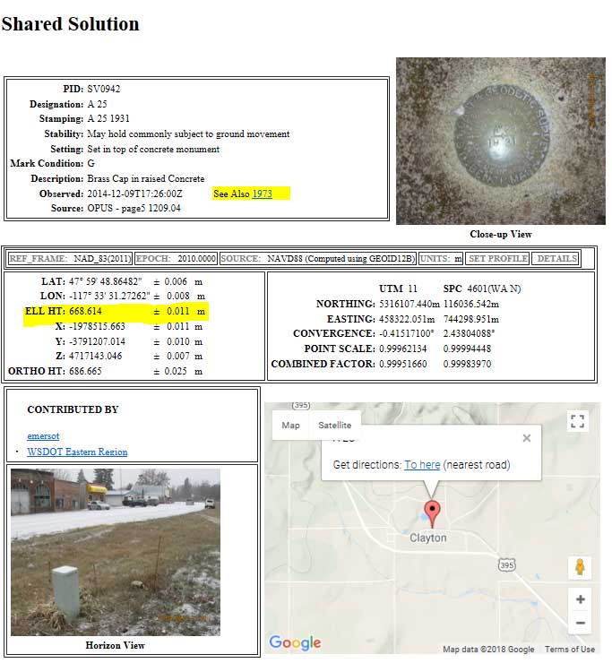
The OPUS Shared station PID SV0942 (A 25) is an example of two OPUS Shared results generating ellipsoid height values that differ by 10 cm. (See yellow highlighted section in the box titled “Differences in OPUS Shared Ellipsoid Heights for PID SV0942.”) This large difference is significant when you performing a survey where you need heights to better than 3 cm (0.1 foot). This is one reason that NGS requires two OPUS Shared solution for every mark used in the development of the hybrid geoid model.
Differences in OPUS Shared Ellipsoid Heights for PID SV0942
Source: National Geodetic Survey
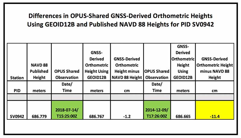
In the OPUS Shared solutions of PID SV0942, the latest OPUS Shared GNSS-derived orthometric heights (2018-07-14) agrees to about a cm with the published NAVD 88 height, while the 2014 Opus Shared GNSS-derived orthometric height is -11.4 cm different from the published NAVD 88 value. (See yellow highlighted section in box titled “Differences in OPUS-Shared GNSS-Derived Orthometric Heights Using GEOID12B and Published NAVD 88 Heights for PID SV0942.”)
Differences in OPUS-Shared GNSS-Derived Orthometric Heights Using GEOID12B and Published NAVD 88 Heights for PID SV0942
Source: National Geodetic Survey
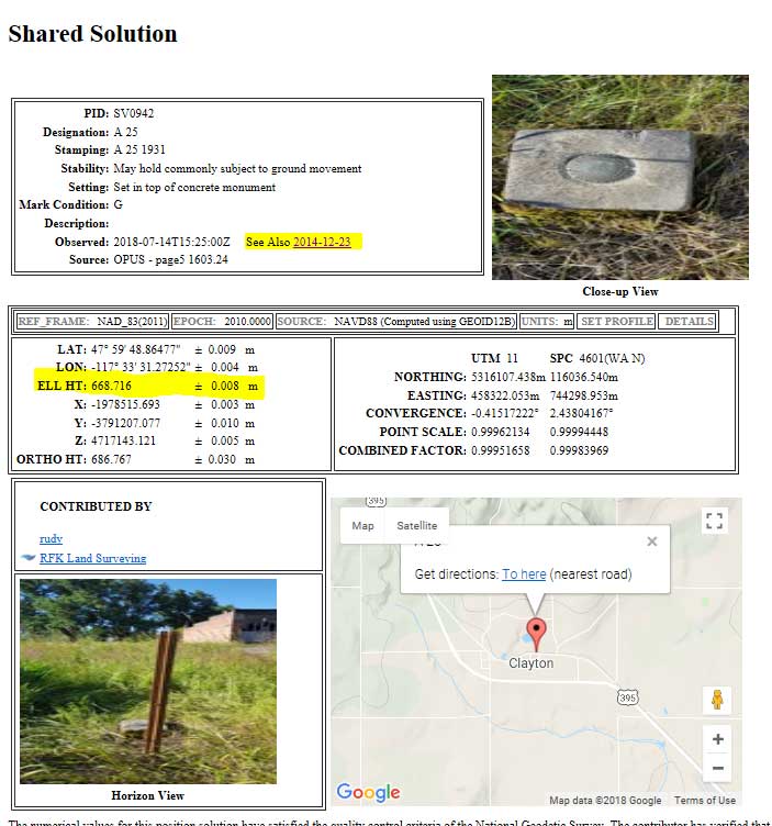
It should be noted that the error estimates provided in the Opus Shared output indicate the ellipsoid heights are good to about +/- 1 cm. (See highlighted section in box titled “Two OPUS Shared Solution for PID SV0942.”) Saying that, the two NAD 83 (2011) ellipsoid heights disagree with each other by 10.2 cm. I like a quote that is attributed to Mark Twain – “It ain’t what you don’t know that gets you into trouble. It’s what you know for sure that just ain’t so.” (Obtained from http://lukefostvedt.com/famous-quotes-about-statistics/). I’m not suggesting that Opus Shared solutions results are incorrect. I’m attempting to provide an example of why users need to repeat all observations and to demonstrate how error estimates can be misleading.
“It ain’t what you don’t know that gets you into trouble.It’s what you know for sure that just ain’t so.”
The number of GPS on Bench Mark stations completed as of July 27, 2018, represents about 30 percent of the total number of stations that need to be observed. As I have explained in previous columns, there are many invalid GPS on BMs stations that may be used in the next hybrid geoid model unless more bench marks with valid NAVD 88 heights are observed with GNSS. NGS will accept data for inclusion in the next hybrid geoid model, GEOID18, until the end of August 2018. After that, NGS’ GPS-on-Bench-Mark Program will expand to include other regions and will focus on data to improve NGS datum transformation tools. This column provided an update and status report on stations observed in support of the 2018 GPS on BMs program, provided an example of how the OPUS Shared results can be used to identify a station that may have moved since it was last leveled, and the importance of repeating OPUS observations. I would encourage users to register for NGS’ next webinar on the GPS on Bench Mark Program scheduled for Thursday, Aug. 9th to hear the latest status of the program.
My last column described the National Geodetic Survey’s (NGS) GPS on Bench Marks (BM) 2018 interactive web map, and provided an update and status report on stations observed in support of the 2018 GPS on BMs Program. It mentioned that all new data received by the cut-off date of Aug. 31 will be analyzed by NGS and, if appropriate, the results will be included in the next hybrid geoid model. This is a great opportunity to provide data that will help to improve the hybrid geoid model in your region. This column will provide an update and status report on stations observed in support of the 2018 GPS on BMs program and provide an example of how OPUS-shared results identified a station that may have moved since it was last leveled.
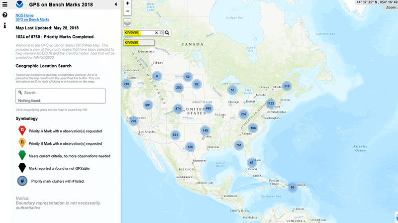
As mentioned in the last column, the GPS on BMs 2018 web page contains a link to a web map where users can determine which bench marks NGS would like users to occupy before the August 31, 2018, deadline. The web map also provides a list of the stations observed to date to ensure users are not wasting their time observing stations that already have enough repeat observations. NGS is updating the map weekly to reduce users occupying stations that already have enough redundant observations. The box titled “2018 Web Map” depicts the map update of May 25, 2018. The web map has a search feature so if the user knew a station’s PID, they could locate the station on the map. The box titled “An Example of Using the Web Map Search Feature” depicts the search feature using PID AW0690 (see highlighted section in the box).
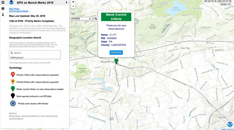
The box titled “Map After Searching for PID KW0690” depicts the map after searching for PID KW0690. As indicated by the symbol, the station meets the current criteria. That is, it has two GNSS-derived ellipsoid heights that agree within NGS’ criteria for use in evaluating and generating the next hybrid geoid model.
Map After Searching for PID KW0690
Click to enlarge.
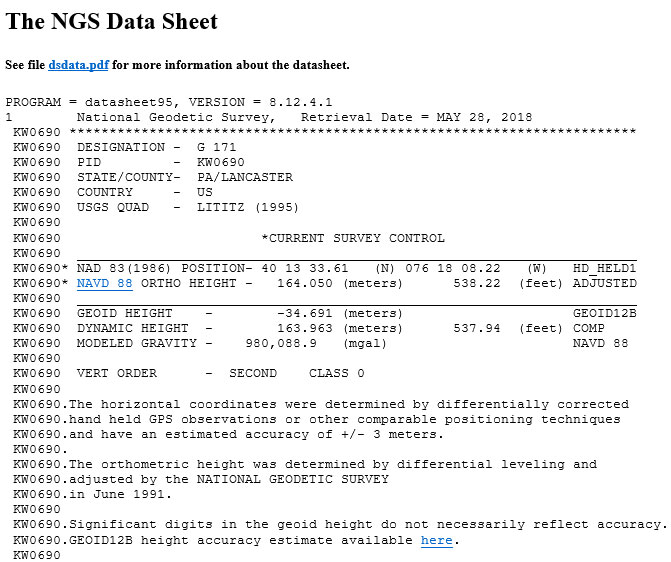
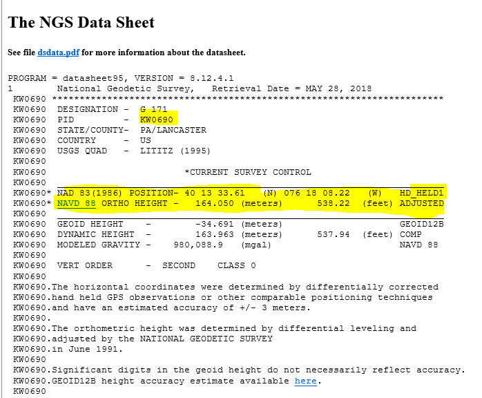
The user can continue to check on the link labeled “Datasheet” to obtain the latest data sheet for the station (see the box titled “NGS Data Sheet for KW0690”).
NGS Data Sheet for KW0690
Click to enlarge.
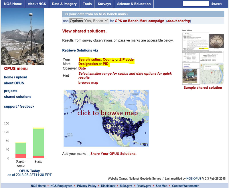
Next, let’s look at the OPUS shared results for the station (KW0690 – G 171). OPUS shared solutions can be found at this website. (see box tilted “OPUS Shared Solutions Web Page”).
OPUS Shared Solutions Web Page
Click to enlarge.
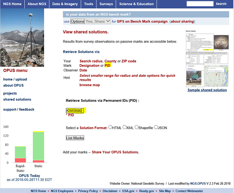
The user can search for a particular OPUS shared solution by checking on the PID option (see highlighted section on the box titled “Web Page After Clicking on PID Option.”
Web Page After Clicking on PID Option
Click to enlarge.
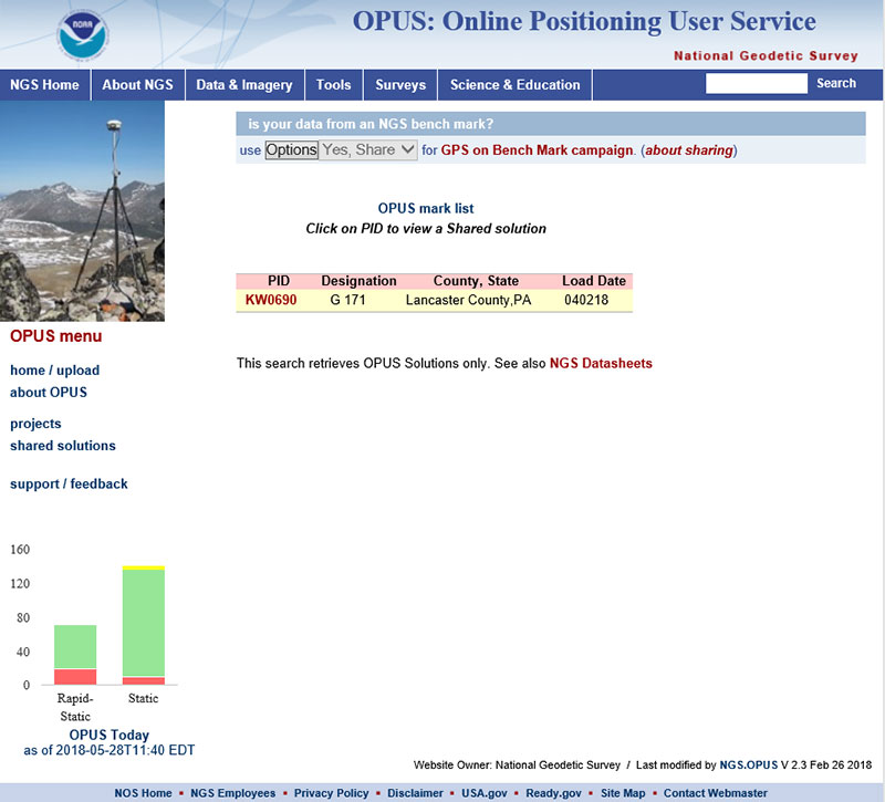
The box titled “An Example of Selecting an OPUS Shared Solution for a PID” depicts the output after clicking on the button labeled “List Marks.”
An Example of Selecting an OPUS Shared Solution for a PID
Click to enlarge.
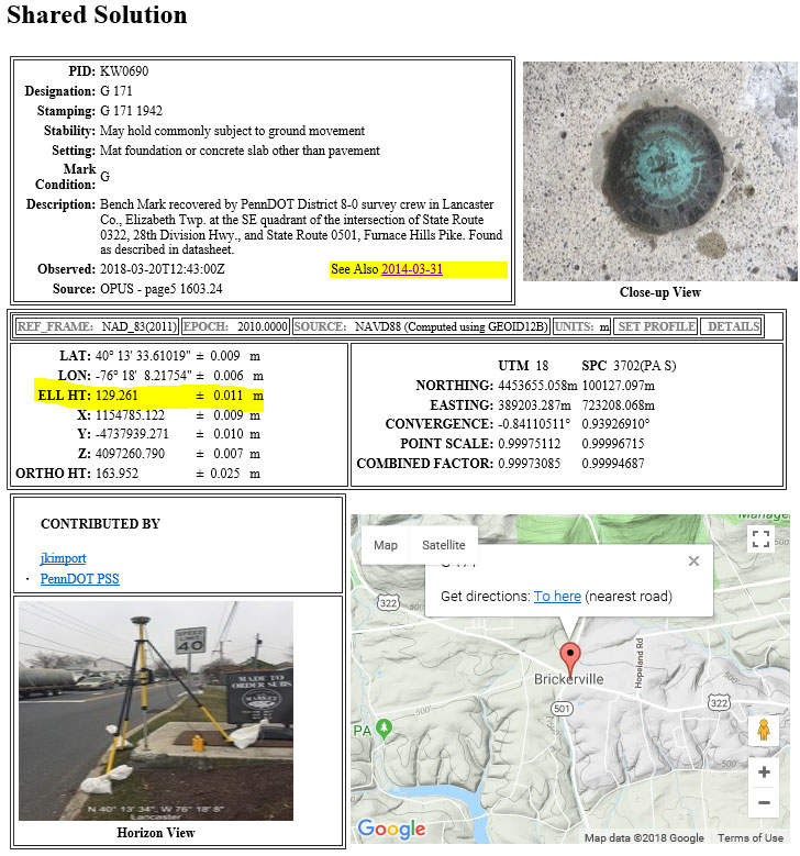
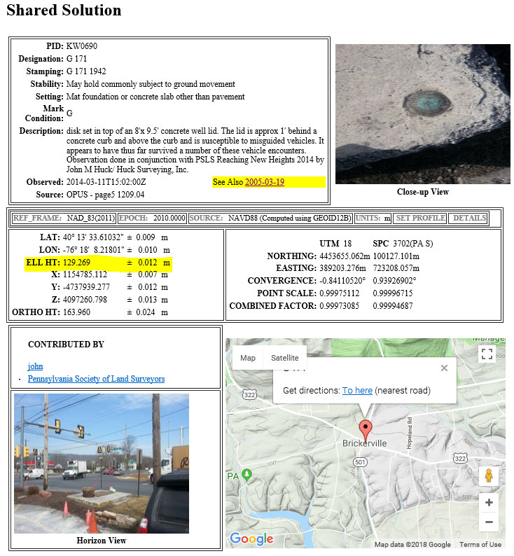
The box titled “The OPUS Shared Solution for KW0690 (2018-03-20)” provides the OPUS Shared solution for station KW0690 performed on March 20, 2018. The output provides the NAD 83 (2011) 2010.0 coordinates with error estimates.
The OPUS Shared Solution for KW0690 (2018-03-20)
Click to enlarge.
When there is more than one observation, the output file provides a link to the other observations. In this case, there was another shared solution on March 31, 2014 (see box titled “The OPUS Shared Solution for KW0690 (2014-03-31).”) The two solutions indicate the ellipsoid heights agree to 8 mm (129.269 m – 129.261 m). This is an indication that the station is a valid candidate to be considered for the development of the hybrid geoid model.
The OPUS Shared Solution for KW0690 (2014-03-31)
Click to enlarge.
The second OPUS Shared solution also indicates that there is a third observation (2005-03-19). Clicking on that link provides the NGS data sheet (see box titled “Excerpt from NGS Data Sheet for KW0690”).
Excerpt from NGS Data Sheet for KW0690
Click to enlarge.
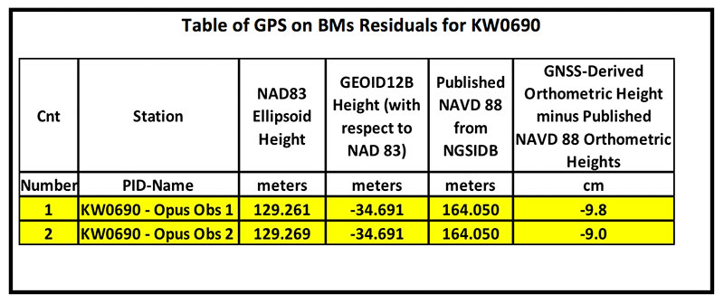
It should be noted that this station doesn’t have a published NAD 83 (2011) coordinate. The OPUS shared solutions provide the NAD 83 (2011) ellipsoid height and the NGS data sheet provides the published NAVD 88 orthometric height. Comparing the GNSS-derived orthometric height using the OPUS shared ellipsoid heights and GEOID12B indicate the station is inconsistent with published NAVD 88 orthometric height. The box titled “Table of GPS on BMs Residuals for KW0690” provides the GPS on BMs residuals based on using the latest hybrid geoid model GEOID12B. It was noted that the two ellipsoid heights agree to within 8 mm but the GNSS-derived orthometric heights using GEOID12B indicate that the two stations disagree with the published NAVD 88 height by almost 10 cm. This may be an indication that the station may have moved since the last time it was leveled. The question that needs to be addressed is should this station be used in the development of the next hybrid geoid model. In my mind, there are basically two school of thought on this topic. One, users that have used this individual station as control would like the hybrid geoid model to provide a GNSS-derived orthometric heights consistent with the published height of this station. If a surveyor followed the appropriate precise leveling procedures to check the validity of the station, that is, performed at least a two-mark leveling tie to ensure that the monument did not move, then they would want the model to be consistent with the published value. Two, if the station moved since it was last leveled, the hybrid geoid model would not provide the most accurate NAVD 88 height.
Table of GPS on BMs Residuals for KW0690
Click to enlarge.
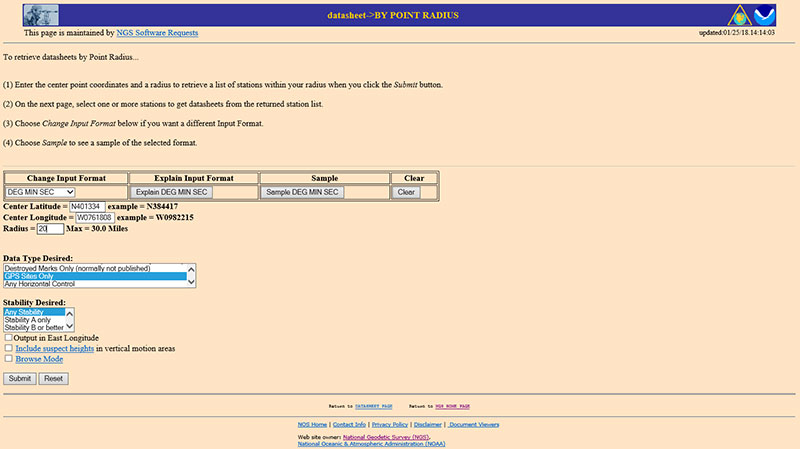
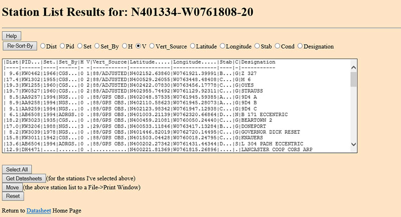
The next step is to analyze the GNSS-derived orthometric height using the latest experimental geoid model. Evaluating GPS on BMs stations nearby station KW0690 will help in determining if the station KW0690 has moved since the last time it was leveled. One way that users can determine stations nearby is to use NGS data sheet retrieval program using the option to retrieve stations by point radius. See box titled “Using NGS Data Sheet Point Radius Retrieval Option for KW0690.” The user enters a latitude and longitude value and a radius search in miles.
Using NGS Data Sheet Point Radius Retrieval Option for KW0690
Click to enlarge.
In this case, I entered the latitude and longitude of station KW0690, a radius of 20 miles (approximately 30 kilometers) and selected the option “GPS Stations Only.” The box titled “Output of NGS Data Sheet Point Radius Retrieval Option for KW0690” provides the output of the search. I sorted the stations by vertical control (“V”)
Output of NGS Data Sheet Point Radius Retrieval Option for KW0690
Click to enlarge.
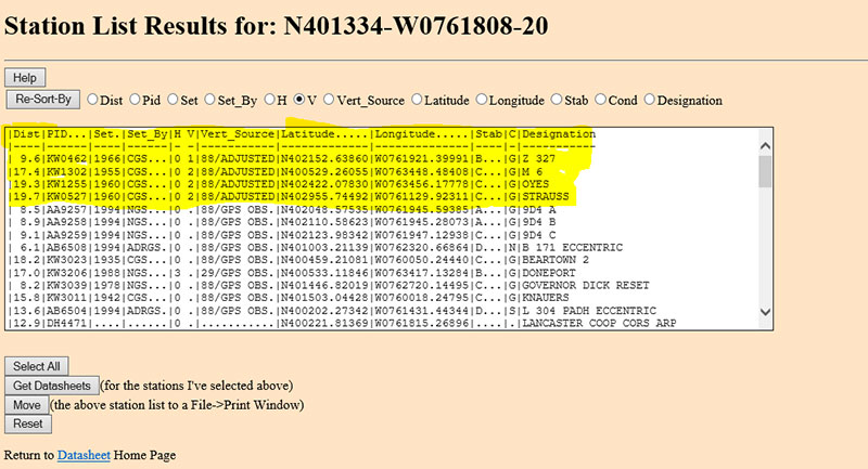
The four bench marks that also have GNSS-derived heights are highlighted in yellow in the box titled “Select the Bench Marks Based on NGS Data Sheet Point Radius Retrieval.” They are all within 20 miles (approximately 30 km) of the station KW0690. By analyzing the GPS on BMs residuals of these nearby stations we can determine if station KW0690 is consistent with its neighbors.
Select the Bench Marks Based on NGS Data Sheet Point Radius Retrieval
Click to enlarge.
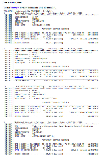
I retrieved the data sheets so I could get their published coordinates for the xGeoid17 web tool. See box titled “Excerpts from Data Sheets Based on NGS Data Sheet Point Radius Retrieval” for the data sheets.
Excerpts from Data Sheets Based on NGS Data Sheet Point Radius Retrieval
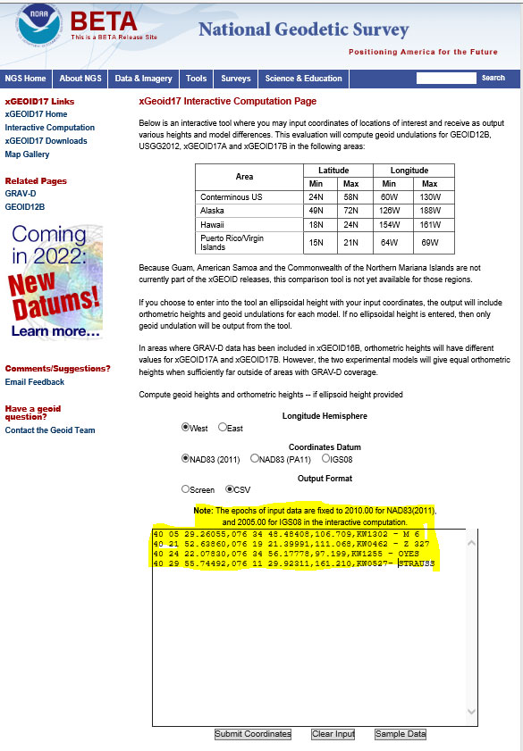
Once you have the stations that are located near the station you’re interested in you can proceed to the xGeoid17 website to obtain the latest information based on the scientific geoid model. I described this procedure in a previous column. See box titled “Using the xGeoid17 Web tool for Stations Nearby KW0690” for an example of the input to the tool.
Using the xGeoid17 Web tool for Stations Nearby KW0690
Click to enlarge.
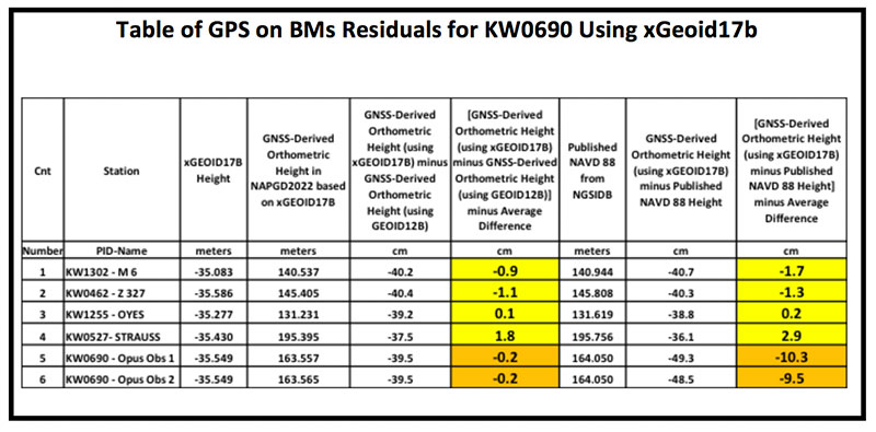
The table titled “Table of GPS on BMs Residuals for KW0690 Using xGeoid17b” provides a summary of the results from the xGeoid17 web page. The procedure used to compute the GPS on BMs residuals has been described in a previous column.
Table of GPS on BMs Residuals for KW0690 Using xGeoid17b
Click to enlarge.
Looking at the column labeled “[GNSS-Derived Orthometric Height (using xGEOID17B) minus Published NAVD 88 Height] minus Average Difference” indicate that the large difference that we noticed using GEOID12B at station KW0690 is also seen using the latest experimental geoid model xGeoid17b. Once again, this is an indication that the station may have moved since it was last leveled.
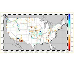
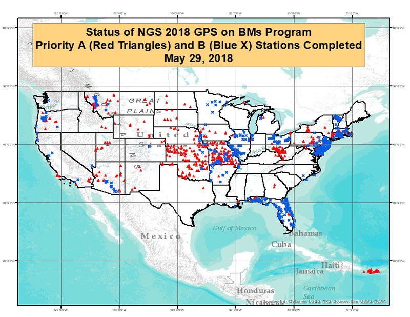
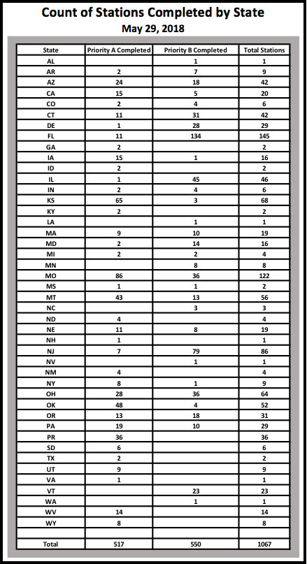
As of May 29, 2018, 1067 of the 5760 priority marks were completed. The box title “Status of NGS 2018 GPS on BMs Program as of May 29, 2018“ is a plot the stations that are labeled as completed and the box titled “Count of Stations Completed by State “ provides the number of stations completed by state. The red triangles are priority A stations completed and the blue “X” are priority B stations labeled as completed.
Status of NGS 2018 GPS on BMs Program as of May 29, 2018
Click to enlarge.
Count of Stations Completed by State May 29, 2018
The number of stations completed as of May 29, 2018, represents about 18.5 percent of the total number of stations that need to be observed. August 31, 2018, is only two months away. According to my latest search of the NGS website (June 3, 2018), 1098 stations are considered done. Hopefully, the number of completed stations will significantly increase during the next last two months. As I have explained in previous columns, there are many invalid GPS on BMs stations that may be used in the next hybrid geoid model unless more bench marks with valid NAVD 88 heights are observed with GNSS. This column provided an update and status report on stations observed in support of the 2018 GPS on BMs program and provided an example of how the OPUS Shared results as identified a station that may have moved since it was last leveled. This is your opportunity to help develop a current, valid hybrid geoid model in your area, and identify NAVD 88 bench marks that have moved since they were last leveled.
The Continuously Operating Reference Station network’s Silver Spring facility will be go offline starting at about 2 p.m. Eastern time Friday, but is expected to be back online by noon Sunday. “Our alternate facility will have full data holdings,” the National Geodetic Survey says on its CORS website.
The shutdown is for a building-wide upgrade. The Online Positioning User Service (OPUS) will be unavailable during the entire shutdown period.
Eric Gakstatter, GPS World’s Survey/GIS editor, has outlined alternatives that surveyors and GIS professionals can use during a shutdown.
I recently was involved in a project outside of the United States. Part of the project involved setting up a couple of RTK base stations. Of course, I wanted the antenna surveyed with reasonable accuracy with respect to ITRF. Even though supporting OPUS outside of the U.S. is out of the scope of the NGS mission (I assume), it works the same outside of the U.S. as it does within the U.S. Ok, somewhat the same.
As you imagine, the network of GPS reference stations outside of the U.S. is not nearly as dense as within the U.S., so you can remove OPUS-RS from the discussion immediately. OPUS-RS only requires a minimum of 15 minutes of data, but there must be three GPS reference stations within 250 km that form a polygon around your occupation point. Obviously, in many parts of the world, you aren’t going to be in a location that meets those specifications. Those requirements can be difficult to meet even in the United States. I recall a project on the West Coast where I had plenty of GPS reference stations within 250 km, but because I was near the Pacific Ocean, I wasn’t within the polygon of three GPS reference stations that OPUS-RS could find.
Back to my ex-U.S. project. With OPUS-RS being out of the consideration, OPUS-S was my choice. What you may not know is that OPUS doesn’t just look at CORS inside the U.S. when post-processing GPS data. It also looks at IGS Stations, which are located all over the world. Granted, I knew the distance to the GPS reference stations would be long, perhaps many hundreds of kilometers to each one, so I planned for long occupation times. This was easy because I was setting up high-quality (choke-ring) permanent antennas on building roofs. I set the GPS receiver to log data overnight at 15-second intervals.
I apologize ahead of time for needing to hide some of the data in order to preserve the privacy of my client, but you can try this same exercise on data you collect, or grab data from an IGS station and chop it into smaller pieces to process.
I logged data for about seven hours. Of course, I had ants in my pants, so I didn’t wait for the rapid orbits (used ultra-rapid), but knew I could reprocess at a later date and use rapid and precise orbits. Here’s what I got:
SOFTWARE: page5 1209.04 master51.pl 072313 START: 2014/01/30 13:49:00
EPHEMERIS: igu17774.eph [ultra-rapid] STOP: 2014/01/30 20:59:30
NAV FILE: brdc0300.14n OBS USED: 3219 / 10519 : 31%
ANT NAME: NONE NONE # FIXED AMB: 39 / 56 : 70%
ARP HEIGHT: 0.0001 OVERALL RMS: 0.015(m)
REF FRAME: IGS08 (EPOCH:2014.0814)
X: xxxxxxx.203(m) 0.396(m)
Y: xxxxxxx.943(m) 0.287(m)
Z: xxxxxxx.554(m) 0.173(m)
LAT: xx xx xx.xxxxx 0.122(m)
E LON: xxx xx xx.xxxxx 0.470(m)
W LON: xx xx xx.xxxxx 0.470(m)
EL HGT: 387.047(m) 0.212(m)
BASE STATIONS USED
PID DISTANCE(m)
xxxxxx 3125832.0
xxxxxx 3743350.2
xxxxxx 3756756.5
Not bad, considering the monster baselines. Yes, that’s 3+ million meters.
I ran the same data set later with better orbits available, as well as more GPS reference data became available.
Wow, the baselines sure improved, and that’s reflected in the solution. That’s because the GPS reference data isn’t immediately accessible from some IGS Stations. In the interest of privacy, I erased the Lat/Lon but kept the elevation. You can see the elevation difference between the two is about 20 cm. I assume it’s an improvement. For confirmation, I decided to run the same dataset through Australia’s AUSPOS online processing service.
X: xxxxxx3.390(m) 0.008(m)
Y: xxxxxx1.676(m) 0.006(m)
Z: xxxxxx9.405(m) 0022(m)
LAT: xxx xx xx.xxxxx
E LON: xxx xx xx.xxxxx
W LON: xxx xx xx.xxxxx
EL HGT: 386.822(m)
The results were comparable to the OPUS solution, differing by 0.7cm in X, 0.08cm in Y and 2.9cm in Z.
AUSPOS used substantially more GPS reference stations (14 total) than OPUS:
STATION, Positional uncertainties (95%) for X, Y, Z (in meters)
Baseline distances ranged from 341 km to 3,700 km.
So, do I believe the OPUS solution or AUSPOS solution? I split the difference at the time. However, I set up the GPS reference stations in such a way that I can access them remotely and log data at any time from my laptop computer, so I’m running a series of eight-hour (or whatever in convenient) occupations and processing them through both services. So yes, OPUS is an international service (shsh, don’t let the bureaucrats and politicians know).
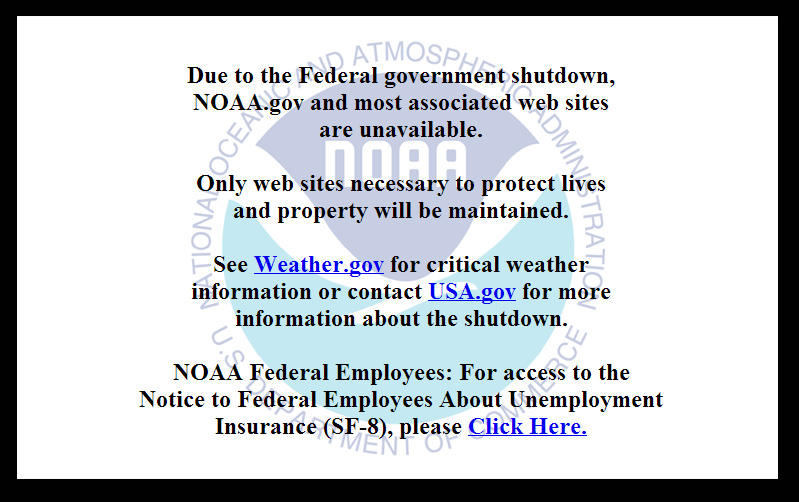
On October 1, 2013, the U.S. federal government shut down and furloughed 800,000 non-essential workers. While services considered essential remained active, those considered non-essential services, like the National Geodetic Survey’s Online Positioning User Service (OPUS), were shutdown. OPUS is a free, online GPS post-processing service. If you try to access www.ngs.noaa.gov, the following screen will be displayed:
Photo: NOAA
For those of you who rely on OPUS for GPS post-processing, now is a great time to try one of the other seven online post-processing services available and not subject to the U.S. federal government. Yes! I wrote seven, and the results from those seven are comparable to OPUS. The other seven, free online GPS post-processing services are:
CSRS-PPP: Canadian Spatial Reference System, Natural Resources Canada
My colleague Mark Silver, creator of the X90-OPUS receiver I wrote about a few months ago, embarked on an effort to run test data through each of the online post-processing services to demonstrate that there are free, online GPS post-processing services available worldwide that produce results comparable to OPUS. The following report is the result of his efforts:
A Comparison of Free GPS Online Post-Processing Services
By Mark Silver
You are probably familiar with the National Geodetic Survey’s OPUS suite of online post processing tools (OPUS-Static, OPUS-Rapid Static and OPUS-Projects.) These services are capable of producing centimeter-level positioning from static GPS observations. What you may not realize is there are at least six viable alternatives to OPUS.
All are free, easy to use, provide world-wide coverage, and generate surprisingly similar results.
Since each uses a unique baseline tool and processing strategies they form an excellent reality check against each other.
IGS orbits and the IGS permanent CORS arrays are used by many of the services, however some use proprietary equipment arrays and orbit products that provide additional redundancy.
How comparable are these services? Which one is the best?
Criteria for Comparing
Comparing results is a difficult proposition:
The true/correct answer for any site is unknown.
What grading scale should be used? Should elevation differences be weighted differently than horizontal differences?
Should the peak-to-peak range or the standard-deviation be prized?
Should comparisons be made on long 24-hour data sets or short 2-hour occupations?
Is a single data set sufficient for a meaningful comparison or are multiple data sets preferable?
Should a service be ‘thrown out’ of consideration because the solutions are substantially different from the mean?
The answer to all of these questions is “it depends.” Your evaluation will depend on your specific application.
For this evaluation, the following rules governed the data set selection:
Choose a site known to be stable with a clean EMI environment.
Use 24-hour observation sets to enable ‘best case’ processing.
Use a sufficiently large data set, 32-consecutive days, to expose trends.
Choose a time period, 90-days in the past, so precise orbits are available to reduce ephemeris effects.
Only consider GPS data.
Use default settings for every option on each processing service.
Scoring
This would not be as interesting without a little competition.
To keep the evaluation simple, the sum of the X, Y and Height range will be the score and the services will be ranked from lowest score to highest score, with the low score being the ‘best.’
Range was chosen as an indicator of the expected maximum error that might be encountered if only a single 24-hour file was observed.
The combined range rewards a processing scheme that best estimates delays, interference, clock errors and other sources of change that occurred during the 32-day trial.
Remember that the every aspect of this ‘competition’ is arbitrary: from the selection of observation sets, to the final scoring system.
The real take-away from this evaluation is not that one service is better, but how close all of the services are to each other.
Two services (JPS’s APPS, magicGNSS) won’t be acceptable to the average user and a third (RTX Centerpoint) may not work for some users based on receiver and antenna support. Details of these problems are presented with the service descriptions below.
The Test Data
SGU1 in St. George, UT USA was chosen as the observation base. The observations consist of 32 consecutive days (May 3, 2013 through June 3, 2013), 24-hour observation files, 30-second interval, GPS only data. The data files were downloaded from the NGS CORS archive.
Each of the 32 files were submitted to each of the processing services and the results have been tabulated for X, Y and Ellipsoid Height. All data is presented in IGS08 current epoch framed coordinates. All data has been projected to UTM Meters for these comparisons.
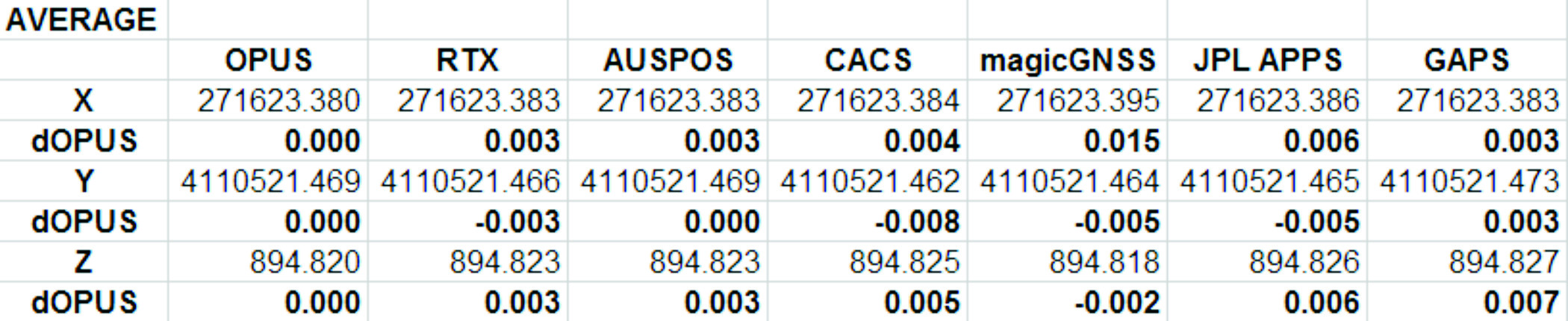
The Average Values
Remember, the real story is how close each of these services produce results to one another. Let’s look at the average positions from each service and the difference from OPUS:
Fig 1: Average Solution Difference from OPUS
As you can see in Figure 1 above, the services were generally within 5mm of OPUS in X, Y and Height.
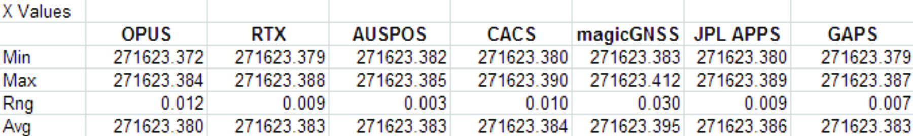
Position Tracking vs. Time
Fig 2: Service Results X vs. Time
Fig 3: Service Results X Range, Average
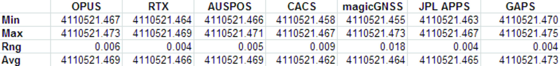
Fig 4: Service Results vs. Time
Fig 5: Service Results Y Range, Average
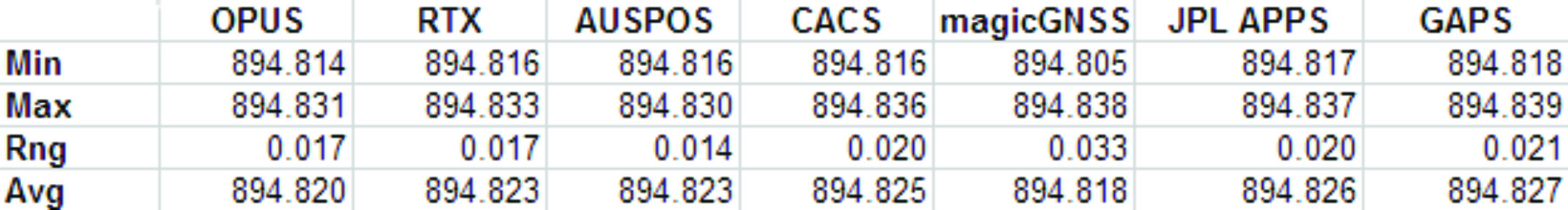
Fig 6: Service Results Z vs. Time
Fig 7: Service Results Z vs. Time
And the Winner Is…
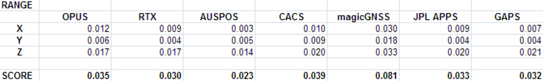
Following are the scores, based on the combination of X, Y and Height range:
Fig 8: The Scores
Score ranking (remember this is just for fun as the services provided remarkably similar results):
AUSPOS
CenterPointRTX
GAPS
APPS
OPUS
CSRS-PPP
magicGNSS
There is a significant issue in the JPL APPS’s reported output positions, which will keep it from being of any use to most users. magicGNSS’s results are significantly different than the other services. User’s should independently evaluate magicGNSS’s suitability for their purpose. SOPAC’s SCOUT could not be evaluated because it patently does not support either the receiver or antenna that was used at the test site.
AUSPOS is a free service from Geoscience Australia. Access is via a simple web interface, the antenna height and type are entered along with a email address for the returned report set. File submission is via FTP or directly from the web interface.
The returned PDF report is the best looking of the reviewed services and includes a Processing Summary showing a map of the CORS sites that were used in the solution. SINEX files are also available.
AUSPOS uses the Bernese GNSS Software for processing baselines, IGS orbits and IGS network stations. Solutions are available for anywhere on the earth.
RINEX files need to be at least 1-hour in length, 6-hour files are recommended. Compact RINEX files are also accepted. Files may be compressed with UNIX, Hatanaka, ZIP, gzip or bzip compression.
Centerpoint RTX Post Processing: Trimble Navigation Limited
CenterPoint RTX Post Processing is a free service offered by Trimble.
It works anywhere in the world and is based on a proprietary Trimble 100+ worldwide CORS network. Accuracy is 2 cm with 1-hour of observation data; 1 cm with 24-hours. Files longer than 24-hours are not accepted.
RTX uses GPS, GLONASS and QZSS tracked SV’s.
The reported output frames include ITRF2008 at current epoch and a user selectable frame like NAD83/2011 2010.0. RTX is one of the few services that will directly export NAD83 framed results.
A single page PDF and a XML result file are returned by RTX. Unfortunately, it is not possible to copy numerical results from the read-only PDF result file to the clipboard.
RTX supports a limited number of receivers (Trimble, Ashtech, Javad, some Leica, some Topcon) and a relatively small subset of IGS modeled antennas. For this test, TEQC was used to stuff the RINEX headers with a comparable Trimble receiver to the actual Ashtech ProFlex 500 receiver that is in use at SGU1. This was all that was required to spoof an accepted device. If the antenna had not been listed, it would have been necessary to spoof the antenna and adjust the height to reflect the difference in L1 phase center offset.
GAPS is an ongoing project at the University of New Brunswick and was developed by the Department of Geodesy and Geomatics Engineering.
File submission is by a web page and GAPS provides a large number of user inputs and potentially allows the highest level of customization of any of the reviewed services:
You may enter a priori coordinates, and a priori constraints
GAPS accepts static or kinematic files
You can set the elevation mask
The Neutral Atmosphere Delay model is selectable
Earth Body Tides and Ocean Tidal Loading can be applied or disabled
GAPS only processes GPS data (no GLONASS.)
Submitted filenames must adhere to the SSSSDDDh.YYt file format. GAPS accepts RINEX and compact RINEX files, they may optionally be gzip, unix compressed or ZIP compressed.
WARNING! APPS only reports the derived position to the nearest decimeter-meter in geographic (lat/lon) coordinates, while reporting ECEF coordinates to a fraction of a millimeter. If you choose to use APPS, you will need to manually convert the ECEF XYZ to geographic coordinates.
JPL’s APPS is based on GIPSY-OASIS (currently version 5). APPS uses NASA’s 70+ Global GPS Network plus densification from other systems (100+ total receivers distributed globally.) Solutions are typically available with 5 seconds delay from observation.
APPS is easy to use, you just specify a file to upload and then click on ‘Upload’ it takes only 15 seconds to get a result after the file upload is complete. You can optionally register for a free account and use email or FTP for bulk uploads.
APPS also has receiver Live Performance Monitoring: (http://www.gdgps.net/monitoring/index.html) which generates a real time graph of three receivers spread through the world.
Before using CSRS-PPP, you will need to register for a free user account.
CSRS has a fantastic desktop application named PPP-Direct that you can just drag and drop files onto. PPP-Direct automatically submits the file and saves all typing, greatly reducing the chance of error.
CSRS-PPP uses both GPS and GLONASS (if available) observables. Ocean Title Loading corrections can be overridden.
CSRS-PPP will accept single frequency files for processing. CSRS will accept RINEX and Compact RINEX, and will decode ZIP, GZIP and unix compression formats.
CSRS-PPP has a fantastic PDF report, a .csv file detailing results epoch by epoch and a great machine readable summary file.
The desktop submission tool, coupled with the great output reports made CSRS-PPP my favorite tool.
magicGNSS accepts emailed files and returns solutions by email. Turnaround time is fast and features a nice PDF report plus SINEX, receiver clock bias files, tropospheric delay, KML trajectory and RINEX CLK clock bias files.
Static and kinematic files with observations from GPS, GLONASS are processed by magicGNSS and the service reportedly Galileo-ready.
magicGNSS uses a subset of IGS stations to provide core coverage.
SCOUT: Scripps Orbit and Permanent Array Center (SOPAC). University of California, San Diego
Scout accepts RINEX and compact RINEX files, compressed (Z, gz, ZIP) submitted from an FTP site or pushed onto a provided FTP server.
Files must be generated on a limited subset of receivers and antennas. While the IGS antenna and receiver files are the basis for acceptable devices, not all IGS-listed devices are on the allowable device list. SCOUT documentation specifically warns against spoofing devices and antennas.
SCOUT uses the GAMIT processing engine.
Because the test data for this article is from a unsupported receiver and the submittal process requires a FTP host server with anonymous access which most users will not bother with, the output from SCOUT was not evaluated.
Conclusion
The similarity of results between all of the services I processed is amazing. That they differ only by millimeters demonstrates the robustness of the algorithms and processes they use.
The difference between AUSPOS, RTX, GAPS, OPUS and CSRS-PPP solutions are negligible. For important positioning projects, it undoubtedly makes sense to use them all.
For locations in the United States, OPUS and RTX return NAD83-2011 framed results. Only OPUS returns derived orthometric heights using GEOID12A. While OPUS has more provenance than the other services, it is easy enough to submit important observations to multiple services as a reality check for important positions.
###
As you read from Mark’s report above, even though OPUS is shut down until the U.S. Congress can resolve its differences, don’t let that stop you from processing your GPS static sessions. However, some level of due diligence on your part is needed as requirements vary for each service. For example, static sessions for the OPUS-RS service can be as short as 15 minutes while other services require two hour GPS static sessions. Furthermore, some services process GPS L1 data while others require both GPS L1 and GPS L2 observations.