Tag: pedestrian

  • Toward a Unified PNT — Part 2

    Toward a Unified PNT — Part 2

    Photo: peeterv/iStock/Getty Images Plus/Getty Images
    Photo: peeterv/iStock/Getty Images Plus/Getty Images

    Ambiguity and Environmental Data: Two Further Key Challenges of Multisensor Positioning

    By Paul D. Groves, Lei Wang, Debbie Walter, and Ziyi Jiang, University College London

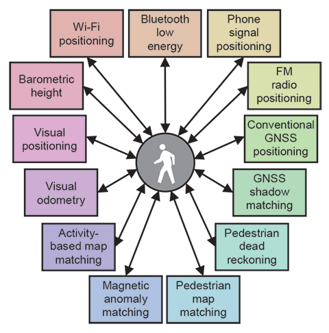
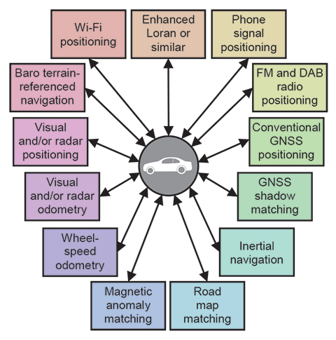
    The coming requirements of greater accuracy and reliability in a range of challenging environments for a multitude of mission-critical applications require a multisensor approach and an over-arching methodology that does not yet exist. Part 1 of this article, in the October issue, examined the two key concepts of complexity and context. In this continuation, we complete our overview with exploration of the requirements of ambiguity and environmental data.

    Ambiguity occurs when measurements can be interpreted in more than one way, leading to different navigation solutions, only one of which is correct. Any navigation technique can potentially produce ambiguous measurements. The likelihood depends on both the positioning method and the context, both environmental and behavioral. Urban and indoor positioning techniques that do not require dedicated infrastructure are particularly vulnerable to ambiguity. Poor handling of ambiguity results in erroneous navigation solutions and the navigation system can become “lost,” whereby it is unable to recover and may even reject correct measurements.

    There are six main causes of ambiguity: feature identification, pattern matching, propagation anomalies, geometry, system reliability, and context ambiguity. Each of these is described in turn below.

    Feature Identification Ambiguity. The proximity, ranging, angular positioning, and Doppler positioning methods all use landmarks for positioning. These may be radio, acoustic, or optical signals, or natural or man-made features of the environment. For reliable positioning, these signals or features must be correctly identified.

    Digital signals intended for positioning incorporate identification codes. However, where a signal is weak and/or interference is high, it may be possible to use the signal for positioning but not decode the identification information. For signals of opportunity — that is, not designed for positioning — the identification codes may be encrypted, while analog signals do not typically have identifiers. These signals must be identified using their frequencies and an approximate user position, in which case there may be multiple candidates. Even where a signal of opportunity is identifiable, the transmission site may change without warning. For example, Wi-Fi access points are sometimes moved and mobile phone networks are periodically refigured. Thus, there is a risk of false landmark identification.

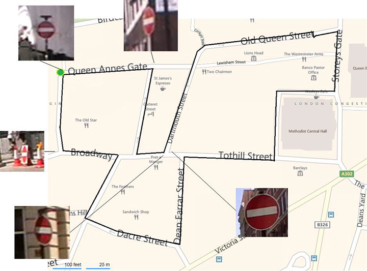
    Environmental features are difficult to identify uniquely. In image-based navigation, man-made features, such as roads, buildings, and signs, are easiest to identify in images due to their line and corner features. However, similar objects are often repeated in relatively close proximity. For example, Figure 18 shows the locations of the five “no entry” signs in a 1,200-meter circuit of Central London streets. Two of the signs are within 20 meters of each other. (Figure numbering continues the sequence beginning in Part 1, October issue.)

    Figure 18. “No entry" signs in a 1,200-meter circuit of Central London. (Background image courtesy of Bing maps | Photo: Paul D. Groves, Lei Wang, Debbie Walter and Ziyi Jiang, University College London)
    Figure 18. “No entry” signs in a 1,200-meter circuit of Central London. (Background image courtesy of Bing maps | Photo: Paul D. Groves, Lei Wang, Debbie Walter and Ziyi Jiang, University College London)

    Pattern-Matching Ambiguity. The pattern-matching positioning method maintains a database of measurable parameters that vary with position. Examples include terrain height, magnetic field variations, Wi-Fi signal strengths, and GNSS signal availability information. Values measured at the current unknown user position are compared with predictions from the database over a series of candidate positions. The position solution is then obtained from the highest scoring candidate(s).

    An inherent characteristic of pattern matching is that there is sometimes a good match between measurements and predictions at more than one candidate position. Figure 19 and Figure 20 show GNSS shadow-matching scoring maps based on smartphone measurements taken at the same location 40 seconds apart. The scores are obtained by comparing GNSS signal-to-noise measurements with signal availability predictions derived from a 3D city model. In Figure 19, maximum scores (shown in dark red) are only obtained in the correct street, whereas in Figure 20, there is also a high-scoring area in the adjacent street, giving two possible position solutions.

    Figure 19. GNSS shadow-matching scoring map – unambiguous case (the cross shows the true position and white areas are indoor locations). (Photo: Paul D. Groves, Lei Wang, Debbie Walter and Ziyi Jiang, University College London)
    Figure 19. GNSS shadow-matching scoring map – unambiguous case (the cross shows the true position and white areas are indoor locations). (Photo: Paul D. Groves, Lei Wang, Debbie Walter and Ziyi Jiang, University College London)
    Figure 20. GNSS shadow-matching scoring map – unambiguous case (the cross shows the true position and white areas are indoor locations). (Photo: Paul D. Groves, Lei Wang, Debbie Walter and Ziyi Jiang, University College London)
    Figure 20. GNSS shadow-matching scoring map – unambiguous case (the cross shows the true position and white areas are indoor locations). (Photo: Paul D. Groves, Lei Wang, Debbie Walter and Ziyi Jiang, University College London)

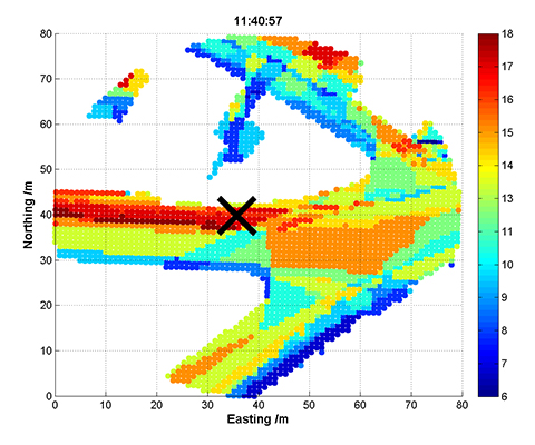
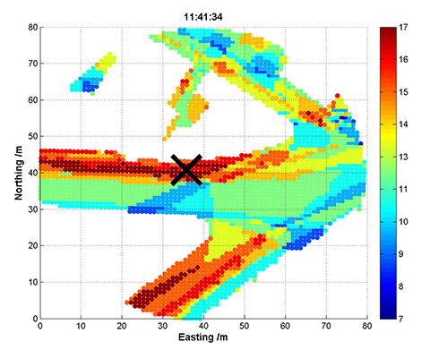
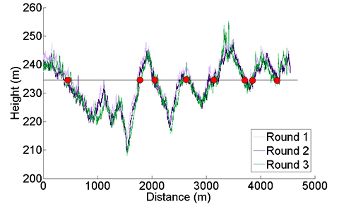
    Figure 21 presents another example, showing the height of a road vehicle derived from a barometric altimeter at three different times. Provided the altimeter is regularly calibrated, it may be used for terrain-referenced navigation (TRN), determining the car’s position along the road by comparing the measured height with a database. However, if only the current height is compared, it will typically match the database at multiple locations within the search area, as the figure shows. The ambiguity can be reduced by comparing a series of measurements from successive epochs, known as a transect, with the database. This approach is applicable to any pattern-matching technique. However, increasing the transect length to reduce the ambiguity also reduces the update rate, and the ambiguity problem can never be eliminated completely.

    Figure 21. Height of a car derived from a barometric altimeter at three different times; readings of around 235 m are highlighted. (Photo: Paul D. Groves, Lei Wang, Debbie Walter and Ziyi Jiang, University College London)
    Figure 21. Height of a car derived from a barometric altimeter at three different times; readings of around 235 m are highlighted. (Photo: Paul D. Groves, Lei Wang, Debbie Walter and Ziyi Jiang, University College London)

    Signal Propagation Anomalies. The ranging, angular positioning, and Doppler positioning methods all make the assumption that the signal propagates from the transmitter (or other landmark) to the user in a straight line at constant speed. Significant position errors can therefore arise when these assumptions are not valid due to phenomena such as non-line-of-sight reception, multipath interference, and severe atmospheric refraction. In challenging environments, such as dense urban areas and indoors, multiple signals are typically affected by propagation anomalies, and it is not always easy to determine which signals are contaminated.

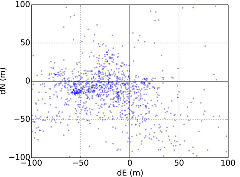
    Where the position solution is overdetermined (that is, more than the minimum number of signals are received), different combinations of signals will produce different position solutions when there are significant propagation anomalies. 

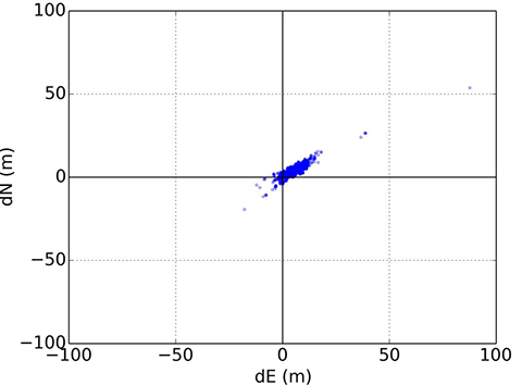
    Figures 22 and 23 illustrate this for conventional GNSS positioning using a Leica Viva geodetic receiver, showing the position errors obtained using different combinations of GPS and GLONASS signals. In Figure 22, the receiver is located on a high rooftop and the majority of position solutions are within 15 meters of the mean, with the remainder easily dismissible as outliers. However, in Figure 23, where the receiver is located in a dense urban location, the candidate position solutions are spread over more than 100 meters, and the correct position solution is not clear. The densest cluster of positions is far from both the centroid and the truth. Therefore, anomalous signal propagation may be treated as an ambiguity problem.

    Figure 22. GNSS position errors using different combinations of signals in a rooftop environment. (Photo: Paul D. Groves, Lei Wang, Debbie Walter and Ziyi Jiang, University College London)
    Figure 22. GNSS position errors using different combinations of signals in a rooftop environment. (Photo: Paul D. Groves, Lei Wang, Debbie Walter and Ziyi Jiang, University College London)
    Figure 23. GNSS position errors using different combinations of signals in a dense urban environment. (Photo: Paul D. Groves, Lei Wang, Debbie Walter and Ziyi Jiang, University College London)
    Figure 23. GNSS position errors using different combinations of signals in a dense urban environment. (Photo: Paul D. Groves, Lei Wang, Debbie Walter and Ziyi Jiang, University College London)

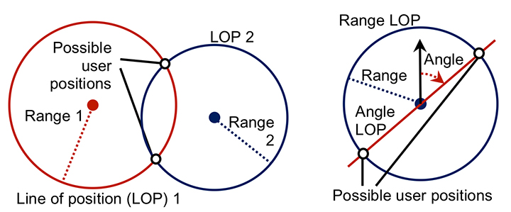
    Geometric Ambiguity. Geometric ambiguity occurs when more than one position solution may be derived from a set of otherwise unambiguous measurements. Figure 24 shows two examples. On the left, two ranging measurements in two dimensions produce circular lines of position that intersect in two places. On the right, a ranging measurement and a direction-finding measurement are made using the same signal. As direction finding has a 180° ambiguity, the lines of position also intersect at two places.

    Figure 24. Geometric ambiguity in two dimensions from two ranging measurements (left), and a ranging and direction-finding measurement (right). (Photo: Paul D. Groves, Lei Wang, Debbie Walter and Ziyi Jiang, University College London)
    Figure 24. Geometric ambiguity in two dimensions from two ranging measurements (left), and a ranging and direction-finding measurement (right). (Photo: Paul D. Groves, Lei Wang, Debbie Walter and Ziyi Jiang, University College London)

    System Reliability. Navigation subsystems can produce incorrect information for a host of different reasons. Some examples include:

    • user equipment hardware and software faults;
    • transmitter hardware and software faults;
    • out-of-date databases used for pattern matching, including TRN, GNSS shadow matching, and map matching;
    • wheel slips in odometry;
    • the effects of passing vehicles and animals on environmental feature visibility, availability and strength of radio signals, and Doppler-based dead reckoning.

    Some of these failure modes are easily detectable through the measurements failing basic range checks or being absent altogether. In other cases, faults may be detected by consistency checks within the subsystem. For example, wheel slip may be detected by comparing measurements from different wheels, while Doppler radar and sonar systems typically incorporate a redundant beam to enable the interruption of a beam by a vehicle or animal to be detected.

    Subsystems can sometimes output incorrect information that is plausible. An ambiguity thus exists where it is uncertain whether or not a measurement may be trusted. An ambiguity also exists where a fault has been detected, but not its source. Thus, some of the information produced by the subsystem must be incorrect, but some of it may be correct.

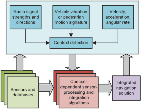
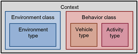
    Context Ambiguity. As discussed in Part 1 of this article (October issue), the optimum way of processing sensor information depends on the context. However, if context information is used, the navigation solution will then depend on the assumed context. For example, if an indoor environment is assumed, indoor radio positioning and map-matching algorithms that are only capable of producing an indoor position solution may be used. Similarly, if an urban environment is assumed, GNSS shadow matching and outdoor map matching may be selected, resulting in an outdoor position solution. Adoption of pedestrian and vehicle motion constraints can also lead to different navigation solutions.

    Context determination is not a completely reliable process. Therefore, to minimize the impact of incorrect context assumptions on the navigation solution, the context should be treated as ambiguous whenever there is significant uncertainty.

    Possible Solutions

    There is no obvious solution to the ambiguity problem. Instead, different approaches to integrating ambiguous information may be adopted depending on the relative priorities of solution availability, reliability, and processing load. The main approaches, illustrated in Figure 25, are discussed below. They all require the subsystems to present the different measurement hypotheses and their associated probabilities to the integration algorithm.

    Figure 25. Methods of handling ambiguous measurements in a navigation integration algorithm. (Photo: Paul D. Groves, Lei Wang, Debbie Walter and Ziyi Jiang, University College London)
    Figure 25. Methods of handling ambiguous measurements in a navigation integration algorithm. (Photo: Paul D. Groves, Lei Wang, Debbie Walter and Ziyi Jiang, University College London)

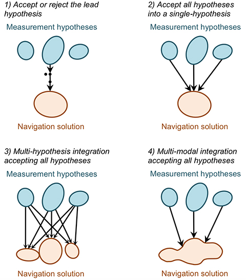
    Accept or reject the lead hypothesis. The simplest way of handling ambiguous information is to maintain a single-hypothesis navigation solution and consider only the most-probable hypothesis from each subsystem. This is then accepted or rejected based on the following criteria:

    • Whether the probability of the highest scoring hypothesis above a certain threshold.
    • Whether the probability of the second-highest scoring hypothesis below a certain threshold.
    • Whether the highest-scoring measurement hypothesis is consistent with the current integrated navigation solution. (Determinable using measurement innovation filtering.)

    Context may be incorporated into this approach by accepting the highest-scoring behavioral and environmental contexts where they meet the above criteria and computing a context-independent navigation solution otherwise.

    This approach is processor-efficient, but high integrity and availability cannot be achieved simultaneously. Low acceptance thresholds provide high reliability by rejecting most erroneous measurements, but low solution availability as many good measurements are also rejected. Conversely, high acceptance thresholds provide availability at the expense of reliability.

    Accept all hypotheses into a single-hypothesis solution. A probabilistic data association filter (PDAF) accepts multiple measurement or context hypotheses, weighting them according to their probabilities, but represents the navigation solution as the mean and covariance of a uni-modal distribution. The measurement update to the state estimation error covariance matrix accounts for the spread in the hypotheses such that the state uncertainties can sometimes increase following a measurement update.

    This approach reconciles the demands of integrity and availability at the price of a moderate increase in processing load. However, the uni-modal navigation solution can sometimes be misleading. For example, if a pattern-matching system determines that the user is equally likely to be in one of two parallel streets, the overall position solution will be midway between those streets.

    Multi-hypothesis integration accepting all hypotheses. Multi-hypothesis integration deals with multiple measurement and context hypotheses by spawning multiple integration filters, one for each hypothesis. Each filter is allocated a probability based not only on the probabilities of the measurements input to it, but also on the consistency of those measurements with the prior estimates of that filter. This consistency-based scoring is essential; otherwise the filter hypothesis that inputs the highest-scoring measurement hypotheses will always dominate, regardless of whether those measurements are consistent across subsystems and successive epochs.

    A fundamental characteristic of multi-hypothesis filtering is that the number of hypotheses grows exponentially from epoch to epoch. This is clearly impractical, so the number of hypotheses is limited by merging the lowest scoring hypotheses into higher scoring neighbors.

    The overall navigation solution is the weighted sum of the constituent filter hypotheses. Each individual filter hypothesis describes a uni-modal distribution. However, the combined navigation solution is multi-modal. Thus, the position probability can be higher in two streets than in the buildings between those streets. This is a clear advantage over the PDAF-based approach, but the processing load is higher.

    Multi-modal integration accepting all hypotheses. A multi-modal filter is not constrained to model the states it estimates in terms of a mean and covariance. This enables it to process multiple measurement and/or context hypotheses and represent the result as a weighted sum of the probability distributions arising from the individual hypotheses. Suitable data-fusion algorithms include the Gaussian mixture filter and the particle filter. A key advantage over multi-hypothesis integration is that measurements may be treated as continuous probability distributions instead of as a set of discrete hypotheses. This enables pattern-matching measurements to be integrated more naturally and offers greater flexibility in handling signal propagation anomalies.

    A Gaussian mixture filter models the probability distribution of the navigation solution as the weighted sum of a series of multi-variate Gaussian distributions. An example is the iterative Gaussian mixture approximation of the posterior (IGMAP) technique, which has been applied to terrain referenced navigation integrated with inertial navigation.

    A particle filter models the probability distribution of the navigation solution using a series of semi-randomly distributed samples, known as particles. Between a thousand and a million particles are typically deployed, with a higher density of particles in higher probability regions of the distribution. Particle filters have been used with a number of different navigation technologies, including TRN, pedestrian map matching, Wi-Fi positioning, and GNSS shadow matching.

    Multi-modal integration algorithms offer the greatest flexibility in reconciling the demands of solution availability and reliability, but also potentially impose the highest processing load.

    Issues to Resolve

    The key challenge in handling ambiguous measurements is determining realistic probabilities for each hypothesis. A probability must also be calculated for the null hypothesis, that is, the hypothesis that every candidate measurement output by the subsystem is wrong. The same applies to ambiguous context.

    A feature identification algorithm must allocate a score to every database feature that it compares with the sensor measurements. In practice, only features within a predefined search area, based on the prior position solution and its uncertainty, will be considered. Features scoring above a certain threshold will be possible matches. Similarly, pattern- matching algorithms allocate a score to each candidate position in the search area according to how well the sensor measurements match the database at that point. For correct handling of ambiguous matches, these scores should be as close as possible to the probabilities of the feature match or candidate position being correct.

    Feature identification and pattern-matching algorithms can also fail to consider the correct feature or candidate position for several reasons. The correct feature or position may be outside the database search area. It may be absent due to the database being out of date. The sensor may also observe or be affected by a temporary feature that is not in the database, such as a vehicle. The null hypothesis probability must account for all of these possibilities. In practice, it will be higher where there is no good match between the measurements and database.

    Signal propagation anomalies affect the error distributions of ranging, angle, and Doppler shift measurements, and the positions and velocities derived from them. These error distributions depend on whether the signals are direct line-of-sight (LOS), non-line-of-sight (NLOS), or multipath- contaminated LOS. However, this is not typically known. Signal strength measurements, environmental context, signal elevation (for GNSS), distance from the transmitter (for terrestrial signals), consistency between different measurements, and 3D city models can all contribute useful information. However, their relationship with the measurement errors is complex, so a semi-empirical approach is needed.

    Moving on to reliability, virtually any subsystem can produce false information. The overall probability will typically be very low and thus only significant for high-integrity applications. However, the failure probability will be higher in certain circumstances, in which case the relevant subsystem should report a higher null probability. For example, in odometry, the probability of a wheel slip depends on host vehicle dynamics. Similarly, a radio signal is more likely to be faulty if it is weaker than normal. Repeated measurements, changes to the update interval, and sudden changes in a sensor output are also indicative of potential faults.

    Geometric ambiguity is easy to quantify as the candidate solutions have equal probability in the absence of additional information.

    As proposed in Part 1, the context determination process should produce multiple context hypotheses, each with an associated probability. Therefore, it is important to ensure that all navigation subsystems that use this context information do so in a probabilistic manner. Thus, where different context hypotheses lead to different values of the measurements output by a navigation subsystem, each measurement hypotheses should be accompanied by a probability derived from the context probabilities.

    A further issue to resolve is the relationship between discrete and continuous ambiguity. Ambiguities in feature identification, solution geometry, failures, and context categorization are discrete and are suited to integration filters that treat them as a set of discrete hypotheses. However, the position solution ambiguity in pattern-matching is continuous, that is, the probability density is a continuous function of position, albeit sampled at discrete grid points. This probability distribution may be input directly to a particle filter. However, if the integration algorithm is a uni-modal filter or a bank of uni-modal filters, the probability distribution must be converted to a set of discrete hypotheses. This can be done by fitting a set of Gaussian distributions to the probability distribution. For signal propagation anomalies, their presence or absence is discrete. However, the resulting measurement error distribution is continuous, so a similar approach is appropriate.

    The same challenging environments that require multiple navigation subsystems to maximize solution availability, accuracy, and reliability can also induce those subsystems to produce ambiguous measurements. Consequently, the modular integration architecture proposed in Part 1 should be capable of handling ambiguous measurements.

    This is discussed further in our IEEE/ION PLANS 2014 paper, “The Four Key Challenges of Advanced Multisensor Navigation and Positioning.”

    Environmental Data

    Position-fixing systems need information about the environment, sometimes known as a “world model,” to operate. Proximity, ranging, and angular positioning all use landmarks that must be identified. For GNSS and other long-range radio systems, identification codes are determined when the system is designed and incorporated in the user equipment. However, this is not practical for shorter range signals, whether opportunistic or designed for positioning, due to the vast numbers of transmitters available worldwide and the fact that many will be installed during the lifetime of the user equipment. The user equipment will also require information on the characteristics of a signal to enable it to use that signal for ranging. A mobile device equipped with a generic radio or transceiver may be required to download software to enable it to use a proprietary indoor positioning system. For environmental feature-matching techniques, the user equipment requires information to enable it to identify each landmark.

    Navigation using landmarks also requires their positions and, for passive ranging, their timing offsets. Signals designed for positioning typically provide this information, but it can take a long time to download (30 seconds for GPS C/A code) and can be difficult to demodulate under poor reception conditions. The positions of opportunistic radio transmitters and environmental features must be determined by other means.

    For positioning using the pattern-matching method, a measurement of radio signal strength or a characteristic of the environment, such as the terrain height or magnetic field, is compared with a database to determine position. Therefore, a database providing values of the measured parameter over a regular grid of positions is required. Map matching requires a map database to indicate where the user can and cannot go. GNSS shadow matching requires a 3D city model to predict signal visibility.

    Finally, as discussed in Part 1 of this article, mapping is required to determine environmental context information from the position solution and to enable location-dependent context connectivity information (for example, the location of train stations) to be used for context determination.

    Possible Solutions

    We discuss in turn the environmental data collection and its distribution to the user equipment.

    Data Collection. Positioning data may be collected either from a systematic survey or by the users. In either case, regular updates will be required. A systematic survey might be conducted by the subsystem supplier, a national mapping agency, or a private third party. The user will need to pay for the data in some way. It could be included in the equipment cost, via a subscription payment, by accepting advertising, or through general taxation (for some national mapping agency data). For mobile devices, such as smartphones, mapping data may be available for some applications, but not others.

    Single-user data collection does not involve user charges, but only provides data for places the user has already visited. A simple approach requires a good position solution to collect mapping data. This can work for applications that normally use GNSS, but require backups for temporary outages. However, it does not work for areas where GNSS reception is poor. Simultaneous localization and mapping (SLAM) techniques can perform mapping without a continuous position solution. However, there are several constraints. First, a good position solution that is independent of the data being mapped is required at some point, usually the start. Second, a navigation system including dead-reckoning technology must be used. Third, locations must be visited repeatedly within a short period of time (to achieve “loop closure”). Finally, only features close to the user can be mapped.

    Cooperative mapping by a group of users solves many of the problems of single-user mapping. It can provide individual users with data for places they have not visited before. Distant landmarks can also be mapped more easily by multiple users, particularly where it is necessary to determine a timing offset as well as the location. However, a method for comparing and combining data from multiple users is required.

    Data Distribution. For data collected by a systematic survey, there are two main data distribution models: pre-loading and streaming. Pre-loading requires sufficient user equipment data storage to cover the area of operation. New data may have to be loaded prior to a change in operating area, and updates will be required. However, a continuous communications link is not needed.

    Streaming requires much less data to be stored by the user and provides up-to-date information, but only where a communications link is available. Although buffering can bridge short outages, navigation data is simply not available for areas without sufficient communications coverage. Continuous streaming can also be expensive. One solution is a cooperative approach using peer-to-peer communications for much of the data distribution. A pair of users traveling in opposite directions along the same route will each have data that is useful to the other. A further possibility is to incorporate local information servers in Wi-Fi access points for exchanging information relevant to the immediate locality. This might be best suited to indoor navigation, where there is an incentive for the building operator to provide the service.

    For data collected by a single user, no data distribution is required other than a back-up. For cooperative data collection by multiple users, a method of data exchange is needed. This can be via a central server, communicating either in real time or whenever the user returns to base. It can also be through peer-to-peer communications or through local information servers, where there is an incentive to provide them.

    Issues to Resolve 

    Standardization is a major part of the data management challenge. A multisensor navigation system will typically incorporate multiple subsystems with data requirements. This might include road or building mapping, radio signal information, terrain height, magnetic anomalies, visual landmarks, and building signal-masking information for GNSS shadow matching. There will be a different standard for each type of data. Furthermore, different subsystem suppliers will often use different standards for the same type of data. This is sometimes done for commercial and/or security reasons, so the data may be encrypted. There may also be technical reasons for different data standards. For example, in image-based navigation, different feature recognition algorithms require different descriptive data.

    Ideally, all navigation data in a multisensor system should be distributed by the same method. This requires agreement of storage and communication protocols that can handle many different data formats, including encrypted proprietary data and future data formats. Open standards for each type of data should also be agreed, noting that consumer cooperative positioning using peer-to-peer communications and/or local information servers is probably only practical with open data formats. Ideally, the standards should be scalable to enable precisions, spatial resolutions, and search areas to be adapted to the available data storage and communications capacity.

    Peer-to-peer data exchange requires a suitable communications link. Bluetooth is the established standard for consumer applications. Classic Bluetooth provides sufficient capacity, but it takes longer to establish a connection than passing pedestrians or vehicles remain within range. Bluetooth low energy can establish a connection quickly, but the data capacity is limited to 100 kbit/s. This is sufficient for some kinds of navigation data, but not others. Professional and military users have more flexibility to select suitable datalinks.

    Finally, establishing local information servers requires both standardization and an incentive for the hosts. Demand would be greater if there were applications beyond navigation and positioning. Possibilities include product information in shops and exhibit information in museums, both of which might be provided more efficiently from a local server than the Internet. For home users to provide local information servers, they would also have to benefit from them, a potential “chicken-and-egg” problem. For military applications, local information servers are a potential security risk and a target for attack.

    Conclusions and Recommendations

    Achieving accurate and reliable navigation in challenging environments without additional infrastructure requires complex multisensor integrated navigation systems. However, implementing them presents four key challenges: complexity, context, ambiguity, and environmental data handling. Each of these problems has been explored and solutions proposed. 

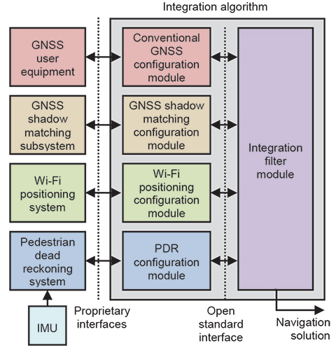
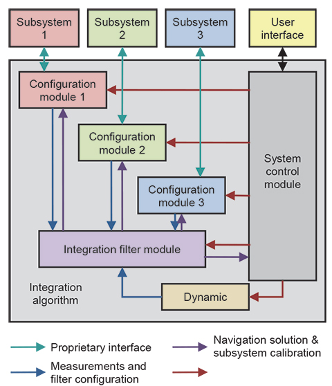
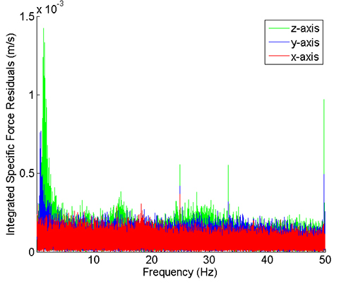
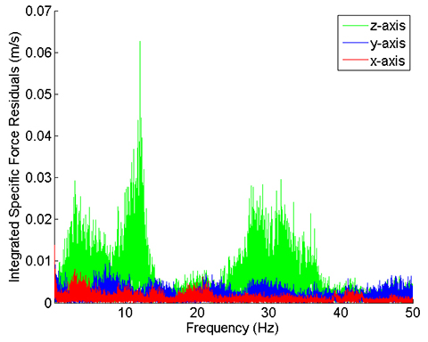
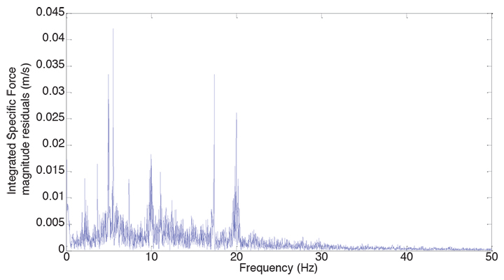
    Conclusions. In Part 1 of this article, a modular integration architecture was proposed to enable multiple subsystems from different organizations to be integrated without the need for whole system expertise or sharing of intellectual property. Furthermore, context-adaptive navigation was proposed to enable a navigation system to respond to changes in the environment and host vehicle (or user) behavior, deploying the most appropriate algorithms. A new probabilistic approach to context determination was proposed and results presented from a number of context detection experiments.

    Here, it has been shown that navigation solution ambiguity can arise from feature identification, pattern matching, propagation anomalies, solution geometry, system reliability issues, and context ambiguity. A number of methods for handling ambiguous measurements in a multisensor navigation system have been reviewed.

    Finally, methods of collecting and distributing data such as locations of radio transmitters and other landmarks, information for identifying signals and landmarks, road or building mapping, terrain height, magnetic anomalies, and building signal-masking information (for GNSS shadow matching) have been discussed.

    Implementing the ideas proposed in this two-part article requires both standardization and further research. Standardization is needed to enable the communication between modules produced by different suppliers of information such as the integrated navigation solution, sensor measurements and characteristics, calibration parameters, performance requirements, context information, mapping, and signal and feature characteristics.

    Further research is needed to support this standardization process, including the identification of a set of fundamental measurement types and their error sources, and the establishment of the best set of context categories for integrated navigation.

    Extensive research into context detection and determination is needed, including the measurements to use, the statistical parameters to derive from those measurements, and a set of context association and connectivity rules.

    An assessment of the different methods for handling ambiguous measurements is needed, comparing accuracy, reliability, solution availability, and processing load. This will enable the community to determine which methods are suited to different applications.

    Finally, there is a need for a practical demonstration of the key concepts proposed in this paper, including modular integration, context adaptivity, ambiguous measurement handling, and collection and distribution of environmental data.


    Paul D. Groves is a lecturer at University College London (UCL), where he leads a program of research into robust positioning and navigation. He is an author of more than 60 technical publications, including the book Principles of GNSS, Inertial and Multi-Sensor Integrated Navigation Systems, now in its second edition. He is a Fellow of the Royal Institute of Navigation and holds a doctorate in physics from the University of Oxford. 

    Lei Wang is a Ph.D. student at UCL. He received a bachelor’s degree in geodesy and geomatics from Wuhan University. He is interested in GNSS-based positioning techniques for urban canyons.

    Debbie Walter is a Ph.D. student at UCL. She is interested in navigation techniques not reliant on GNSS, multi-sensor integration, and robust navigation. She has an MSci from Imperial College London in physics and has worked as an IT software testing manager.

    Ziyi Jiang was a postdoctoral research associate at UCL until 2014, working on urban GNSS and other projects. He holds a bachelor’s degree in engineering from Harbin University and a Ph.D. in rail positioning from UCL. He now works in finance.

    All authors are members of UCL Engineering’s Space Geodesy and Navigation Laboratory (SGNL).

  • Toward a Unified PNT — Part 1

    Toward a Unified PNT — Part 1

    Photo: peeterv/iStock/Getty Images Plus/Getty Images
    Photo: peeterv/iStock/Getty Images Plus/Getty Images

    Complexity and Context: Key Challenges of Multisensor Positioning

    By Paul D. Groves, Lei Wang, Debbie Walter, Henry Martin, and Kimon Voutsis, University College London

    The next generation of navigation and positioning systems must provide greater accuracy and reliability in a range of challenging environments to meet the needs of a variety of mission-critical applications. No single navigation technology is robust enough to meet these requirements on its own, so a multisensor solution is required. Four key challenges must be met: complexity, context, ambiguity, and environmental data handling.

    Although many new navigation and positioning methods have been developed in recent years to address GNSS shortcomings in terms of signal penetration and interference vulnerability, little has been done to bring them together into a robust, reliable, and cost-effective integrated system.

    New positioning techniques investigated over the past 15 years include:Wi-Fi; ultra-wideband; phone signals; television and other signals of opportunity; Bluetooth; lasers, and dead reckoning; pedestrian dead reckoning (PDR) using step detection; pedestrian and activity-based map matching; magnetic anomaly matching; and GNSS shadow matching.

    There have also been improvements to existing technologies: visual navigation, dead-reckoning algorithms, micro-electro-mechanical systems, inertial sensing with cold-atom technology, nuclear magnetic resonance gyros, distance-measuring equipment, Loran, Doppler with Iridium, multiple GNSS constellations, network assistance, and augmentation by commercial pseudolite systems.

    In the next generation, a universal navigation system might be expected to provide position within 3 meters at any location with a very high reliability. No single positioning technology is capable of meeting the most demanding application requirements. Radio signals may or may not be subject to obstruction, attenuation, reflection, jamming, and/or interference. Known environmental features, such as signs, buildings, terrain height variation, and magnetic anomalies, may or may not be available for positioning. The system could be stationary, carried by a pedestrian, or on any type of land, sea, or air vehicle. Furthermore, for many applications, the environment and host behavior are subject to change. A multisensor solution is thus required.

    A robust, reliable, and cost-effective integrated system must meet four key challenges:

    Complexity. How to find the necessary expertise to integrate a diverse range of technologies, how to combine technologies from different organizations that wish to protect their intellectual property, how to incorporate new technologies and methods without having to redesign the whole system, and how to share development effort over a range of different applications.

    Context. How to ensure that the navigation system configuration is optimized for the operating environment and host vehicle (or pedestrian) behavior when both are subject to change.

    Ambiguity. How to handle multiple hypotheses, including measurements of non-unique environmental features, pattern-matching fixes where the measurements match the database at multiple locations, and uncertain signal properties, such as whether reception is direct or non-line-of-sight (NLOS).

    Environmental Data Handling. How to gather, distribute, and store the information needed to identify signals and environmental features and define their points of origin or spatial variation.

    Complexity

    Achieving robust positioning in challenging environments potentially requires a large number of subsystems. For example, Figure 1 shows the possible components of a pedestrian navigation system using sensors found in a typical smartphone. Figure 2 shows possible components of a car navigation system using equipment already common on cars and other suitable low-cost sensors. Some technologies are common to the two platforms, while others differ.

    Figure 1. Potential components of a pedestrian navigation system using smartphone sensors. (Photo: Paul D. Groves, Lei Wang, Debbie Walter, Henry Martin, and Kimon Voutsis, University College London)
    Figure 1. Potential components of a pedestrian navigation system using smartphone sensors. (Photo: Paul D. Groves, Lei Wang, Debbie Walter, Henry Martin, and Kimon Voutsis, University College London)
    Figure 2. Potential components of a car navigation system using commonly available equipment and other low-cost sensors. (Photo: Paul D. Groves, Lei Wang, Debbie Walter, Henry Martin, and Kimon Voutsis, University College London)
    Figure 2. Potential components of a car navigation system using commonly available equipment and other low-cost sensors. (Photo: Paul D. Groves, Lei Wang, Debbie Walter, Henry Martin, and Kimon Voutsis, University College London)

    Any multisensor navigation or positioning system needs integration algorithms to obtain the best overall position solution from the constituent subsystems. These algorithms must not only input and combine measurements from a wide range of subsystems, but also calibrate systematic errors in those subsystems. Designing the integration algorithms therefore requires expertise in all of the subsystems, which can be difficult to establish in a single organization. The more subsystems there are, the more of a problem this is.

    The expert knowledge problem is compounded by the fact that different modules in an integrated navigation system are often supplied by different organizations, who may be reluctant to share necessary design information if this is considered to be intellectual property that must be protected. In a typical smartphone, one company supplies the GNSS chip, another supplies the Wi-Fi positioning service, a third organization supplies the mapping, the network operator provides the phone-signal positioning, a fifth company provides the inertial and magnetic sensors, and a sixth company produces the operating system. Because of lack of cooperation between these different organizations, useful information gets lost. For example, GNSS pseudo-range measurements are not normally available to application developers.

    A further issue is reconfigurability. To minimize development costs, manufacturers share algorithms and software across different products, incorporating different subsystems. They also want to minimize the cost of adding new sensors to a product to improve performance. Similarly, researchers want to compare different combinations of subsystems. However, with a conventional system architecture, modifications must be made throughout the integration algorithm each time a subsystem is added, removed, or replaced. The more subsystems there are, the more complex this task becomes.

    For a given application, different subsystems may also be used at different times. For example, a smartphone may use Wi-Fi positioning indoors and GNSS outdoors and may deploy different motion constraints and map matching algorithms, depending on whether the device is carried by a pedestrian or traveling in a car. Different integration algorithms for different configurations are more processor efficient, but also require more development effort. Conversely, an all-subsystem integration algorithm is quicker to develop, but can waste processing resources handling inactive subsystems.

    Modular Integration. The solution to these problems is a modular integration architecture, consisting of a universal integration filter module and a set of configuration modules, one for each subsystem. The integration filter module would be designed by data fusion experts without the need for detailed knowledge of the subsystems. It would accept a number of generic measurement types, such as position fixes and pseudo-ranges, with associated metadata. The configuration modules would be developed by the subsystem suppliers and would convert the subsystem measurements into a format understood by the filter module and supply the metadata. They would also mediate the feedback of information from the integration filter to the subsystems. The metadata comprises the additional information required to integrate the measurements such as

    • the measurement type and any coordinate frame(s) used.
    • a sensor identification number (to distinguish measurements of the same type from different sensors).
    • statistical properties of the random and systematic measurement errors.
    • identification numbers and locations of transmitters and other landmarks.

    A key advantage of this approach is that subsystems may be changed without the need to modify the integration filter. Provided the new subsystem is compatible, all that is needed is the corresponding configuration module.

    Figure 3 shows an example of a modular integration architecture for a combination of conventional GNSS positioning, GNSS shadow matching, Wi-Fi positioning, and PDR. As well as providing measurements and associated statistical data to the integration filter module, the configuration modules feedback relevant information to the subsystems. Shadow matching works by comparing measured and predicted signal availability over a number of candidate positions, so requires a search area to be specified using other positioning technologies. PDR uses information from other sensors, where available, to calibrate the coefficients of its step length estimation model and correct for heading drift. Conventional GNSS positioning can also benefit from position and velocity aiding to support acquisition and tracking of weak signals in indoor and urban environments.

    Figure 3. Modular integration of conventional GNSS, shadow matching, PDR, and Wi-Fi positioning for pedestrian navigation (different colors denote potentially different suppliers). (Photo: Paul D. Groves, Lei Wang, Debbie Walter, Henry Martin, and Kimon Voutsis, University College London)
    Figure 3. Modular integration of conventional GNSS, shadow matching, PDR, and Wi-Fi positioning for pedestrian navigation (different colors denote potentially different suppliers). (Photo: Paul D. Groves, Lei Wang, Debbie Walter, Henry Martin, and Kimon Voutsis, University College London)

    In principle, each subsystem configuration module could simply supply a position fix to the integration filter module with an associated error covariance. However, other forms of measurement generally give better results. For conventional GNSS positioning, the advantages of tightly coupled (range- domain) integration over loosely coupled (position-domain) are well known.

    PDR is a dead-reckoning technique, so measures distance traveled rather than position. Consequently, providing measurements of position displacement and direction can avoid cumulative errors in the measurement stream.

    GNSS shadow matching and some types of Wi-Fi positioning use the pattern-matching positioning method. This scores an array of candidate position solutions according to the match between the measured and predicted signal availability or signal strength. Although the output of these algorithms is in the position domain, a likelihood distribution can provide more information for the integration filter than a simple mean and covariance.

    Other navigation and positioning techniques generate further types of measurement, including velocity, attitude, specific force, angular rate, range rate, and bearings and elevations of features. The types of measurement depend on the positioning method.

    A universal integration filter must operate without prior knowledge of which measurements it must process and which states it must estimate. Consequently, it must reconfigure its measurement vector, state vector, and associated matrices according to the measurements available, using the metadata supplied by the configuration module. This capability is sometimes called “plug and play,” and a number of prototypes have been developed by different research groups.

    The integration filter must be capable of implementing either error-state or total-state integration, depending on the measurements available. In error-state integration, one of the subsystems, such as inertial navigation, provides a reference navigation solution. The integration filter estimates corrections to that solution using the measurements from other subsystems. In total-state integration, the integration filter estimates the position and velocity directly, and an additional configuration module provides information on the host vehicle (or pedestrian) dynamics.

    Modular integration algorithms could form part of a wider modular integrated navigation concept in which subsystem hardware and software is shared across a range of applications.

    Issues to Resolve

    A critical requirement for the successful implementation of modular integration is an open-standard interface for communication between the universal filter and configuration modules. This enables modules produced by different organizations to work together. To realize the full benefits of modular integration, in terms of interoperability and software re-use, there should be a single standard covering the consumer, professional, research, and military user communities and spanning all of the application domains air, sea, land, indoor, underwater, and so forth. A standard developed by one group in isolation is unlikely to meet the needs of the whole navigation and positioning community, while the development of multiple competing standards defeats the main purpose of modular integration.

    This interface should be defined in terms of fundamental measurement types, such as position, velocity, and the ranges, bearings, and elevations of signals and features. However, there are many different coordinate systems that may be used and positioning may be in 2 or 3 dimensions, while ranging measurements may be true ranges or pseudoranges. Ranging and angular positioning measurements may be differenced across transmitters or landmarks, differenced across receivers or sensors, or double differenced across both.

    A universal interface must support every measurement type that requires different processing by the filter module. However, it need not support formats that are easily convertible. Thus, there is no need to support both the north, east, down, and east, north, up conventions. There are two main approaches to defining the fundamental measurement types:

    • A minimal number of very generic measurement types with metadata used to describe how these should be processed by the integration filter.
    • A large number of more specific measurement types for which the processing methodology is already known.

    For each measurement type, an error specification must be defined. For error sources assumed to be white, a standard deviation or power spectral density (PSD) is required. For correlated errors, such as biases, information on the time correlation is required alongside variances and covariance information. The interface standard should include every conceivable error source. Unused errors can simply be zeroed. The filter module should then use the error specification to determine which error sources to model and how.

    Obtaining reliable navigation sensor error specifications can be difficult. Manufacturers often provide only limited information, while performance in the field can be different from that in the laboratory due to vibration and electromagnetic interference. For new positioning techniques, the error behavior may not be fully understood, while complex error behavior can be difficult to measure. Adaptive estimation techniques provide only a partial solution. Even where the error behavior is well known, it can be too complex to practically model within the estimation algorithm. This could represent a fifth challenge.

    For subsystems used as the reference in an error-state integration filter, such as an inertial navigation system (INS), the errors will typically be correlated across the different components of the subsystem navigation solution, for example position, velocity, and attitude. Furthermore, to represent the error behavior within an integration algorithm, it is necessary to model the error properties of the underlying sensors, accelerometers and gyroscopes in the case of inertial navigation. Thus, it is likely that additional compound measurement types for reference system data will be needed.

    For pseudorange measurements, an issue to consider is the synchronization of different transmitter and receiver clocks. Clocks in receivers for different types of signal, such as GNSS and Loran, may or may not be synchronized with each other. Also, the transmitter clocks are typically synchronized in groups. For example, the GPS satellite clocks are synchronized with each other, as are the GLONASS satellite clocks, but GLONASS is not currently synchronized with GPS. For optimal integration of pseudoranges from different sources, this information must be conveyed to the integration filter.

    The interface standard for communication between the filter and configuration modules must also support feedback of information from the integration filter to the subsystems, via the configuration modules. The integrated position, velocity, and attitude solution, with its associated error covariance, is useful for aiding many different subsystems. Therefore, a generic standard for this should be defined. Conversely, the feedback to the subsystems of calibration parameters estimated by the integration algorithm is sensor specific, so should be incorporated in the definitions of the fundamental measurement types.

    The user requirements, such as accuracy, integrity, continuity, solution availability, update rate, and power consumption, can vary greatly between applications. For example, accuracy is important for surveying, integrity for civil aviation, solution availability for many military applications, and power consumption for many consumer applications. This impacts the design of the whole navigation system. Different modules could be used for different applications. However, it is more efficient if the components adapt to different environments. Figure 4 shows how requirements information can be disseminated in a modular integrated navigation system.

    Figure 4. Modular integration architecture incorporating requirements. (Photo: Paul D. Groves, Lei Wang, Debbie Walter, Henry Martin, and Kimon Voutsis, University College London)
    Figure 4. Modular integration architecture incorporating requirements. (Photo: Paul D. Groves, Lei Wang, Debbie Walter, Henry Martin, and Kimon Voutsis, University College London)

    An open-standard interface specification should be able to handle any conceivable navigation and positioning system. However, it is more efficient if the components adapt to different environments. Similarly, there will be differences in the error magnitudes that an integration filter can handle and in its capability to handle non-Gaussian error distributions. Variations in fault detection and integrity monitoring capability can also be expected. Consequently, there must be a capability specification for each filter module and a protocol for handling mismatches between the measurements and the filter module, and a means to certify that a filter module actually has the claimed capabilities. (Further discussion of modular integration may be found in our IEEE/ION PLANS 2014 paper, “The Four Key Challenges of Advanced Multisensor Navigation and Positioning,” and the Journal of Navigation paper, “The Complexity Problem in Future Multisensor Navigation and Positioning Systems: A Modular Solution.”)

    Context

    Context is the environment that a navigation system operates in and the behavior of its host vehicle or user. Examples include a pedestrian walking (behavior) in an urban street (environment), a car driving at highway speeds on an open road, and an airliner flying high above an ocean.

    Context is critical to the operation of a navigation or positioning system. The environment affects the types of signals available. For example, GNSS reception is poor indoors while Wi-Fi is not widely available outside towns and cities. In underwater environments, most radio signals cannot propagate so acoustic signals are used instead. Processing techniques can also be context dependent. For example, in open environments, non-line-of-sight (NLOS) reception of GNSS signals or multipath interference may be detected using consistency checking techniques based on sequential elimination. However, in dense urban areas, more sophisticated algorithms are required and may be enhanced using 3D city models. GNSS shadow matching only works in outdoor urban environments.

    Navigation using environmental feature matching is inherently context-dependent as different types of feature are available in different environments. Suitable algorithms, databases, and sensors must be selected. For example, terrain referenced navigation (TRN) uses radar or laser scanning in the air, sonar or echo sounding at sea, and barometric pressure on land. Map matching requires different approaches for cars, trains, and pedestrians. Similarly, algorithms and databases for image-based navigation depend on the types of feature available, which vary with the environment.

    Behavioral context is also important and can contribute additional information to the navigation solution. For example, cars normally remain on the road, effectively removing one dimension from the position solution. Their wheels also impose constraints on the way they can move, reducing the number of inertial sensors required to measure their motion. Similarly, PDR using step detection depends inherently on the characteristics of human walking. Using PDR for vehicle navigation or vehicle motion constraints for pedestrian navigation will produce errors.

    Host vehicle behavior is also important for tuning the dynamic model within a total-state navigation filter and for detecting faults through discrepancies between measured and expected behavior. Within a GNSS receiver, the behavior can be used to set tracking loop bandwidths and coherent correlator accumulation intervals, and to predict the temporal variation of multipath errors. The antenna placement on a vehicle or person can also affect performance.

    Historically, context was implicit; a navigation system was designed to be used in a particular type of vehicle, handling its associated behavior and environments. However, many navigation systems now need to operate in a variety of different contexts. For example, a smartphone moves between indoor and outdoor environments and can be stationary, on a pedestrian, or in a vehicle. Similarly, a small surveillance drone may operate from above, amongst buildings, or even indoors. At the same time, most of the new positioning techniques developed to enable navigation in challenging environments, are context-dependent. To make use of these techniques in practical applications (as opposed to research demonstrators), it is necessary to know the context.

    Context-Adaptive Navigation

    The solution to the problem of using context-dependent navigation techniques in variable-context applications is context-adaptive navigation. As shown in  Figure 5, the navigation system detects the current environmental and behavioral context and, in real time, reconfigures its algorithms accordingly. For example, different radio positioning signals and techniques may be selected, inertial sensor data may be processed in different ways, different map-matching algorithms may be selected, and the tuning of the integration algorithms may be varied.

    Figure 5. A context-adaptive navigation system. (Photo: Paul D. Groves, Lei Wang, Debbie Walter, Henry Martin, and Kimon Voutsis, University College London)
    Figure 5. A context-adaptive navigation system. (Photo: Paul D. Groves, Lei Wang, Debbie Walter, Henry Martin, and Kimon Voutsis, University College London)

    Previous work on context-adaptive navigation and positioning focused on individual subsystems and concerned either behavioral or environmental context, not both.

    For example, there has been substantial research into classifying pedestrian motion using inertial sensors to enable PDR algorithms using step detection to estimate the distance travelled from the detected motion. The context information may also be used for non-navigation purposes.

    Typically, orientation-independent signals are generated from the accelerometer and gyro outputs. Statistics such as the mean, standard deviation, root mean squared (RMS), inter-quartile range, mean absolute deviation, maximum−minimum, maximum magnitude, number of zero crossings, and number of mean crossings are then determined from a few seconds of data. Frequency-domain statistics may also be used. Finally, a pattern recognition algorithm is used to match these parameters to the stored characteristics of different combinations of activity types and sensor locations.

    Detection of road-induced vibration using accelerometers has been used to determine whether or not a land vehicle is stationary, while a calibrated yaw-axis gyro can be used to determine when a vehicle is travelling in a straight line. Indoor and outdoor environments may be distinguished using GNSS carrier-power-to-noise-density ratio (C/N0 ) measurements. Wi-Fi signals might also be used for environmental context detection.

    Context Detection Experiments

    We have conducted a number of different context-detection experiments using GNSS, Wi-Fi, and accelerometers. Full details are presented in our ION GNSS+ 2013 paper, “Context Detection, Categorization and Connectivity for Advanced Adaptive Integrated Navigation,” and in our PLANS 2014 paper. Here, some highlights from the results are presented.

    GNSS. GNSS data was collected at five locations inside and immediately outside UCL’s Grant Museum of Zoology; these are shown in Figure 6. C/N0 measurement data was collected from all GPS and GLONASS signals received by a Samsung Galaxy S3 Android smartphone. About 60 seconds of data was collected at each site. Figure 7 presents histograms of the C/N0 measurements and Table 1 lists the means and standard deviations.

    Figure 6. Locations for the GNSS indoor/outdoor context detection experiment. (Photo: Paul D. Groves, Lei Wang, Debbie Walter, Henry Martin, and Kimon Voutsis, University College London)
    Figure 6. Locations for the GNSS indoor/outdoor context detection experiment. (Photo: Paul D. Groves, Lei Wang, Debbie Walter, Henry Martin, and Kimon Voutsis, University College London)
    Figure 7. GNSS C/N0 measurement distributions at sites inside and immediately outside UCL’s Grant Museum of Zoology. (Photo: Paul D. Groves, Lei Wang, Debbie Walter, Henry Martin, and Kimon Voutsis, University College London)
    Figure 7. GNSS C/N0 measurement distributions at sites inside and immediately outside UCL’s Grant Museum of Zoology. (Photo: Paul D. Groves, Lei Wang, Debbie Walter, Henry Martin, and Kimon Voutsis, University College London)
    Table 1. Means and standard deviations of GNSS C/N0 measurements inside and outside UCL’s Grant Museum of Zoology. (Photo: Paul D. Groves, Lei Wang, Debbie Walter, Henry Martin, and Kimon Voutsis, University College London)
    Table 1. Means and standard deviations of GNSS C/N0 measurements inside and outside UCL’s Grant Museum of Zoology. (Photo: Paul D. Groves, Lei Wang, Debbie Walter, Henry Martin, and Kimon Voutsis, University College London)

    As expected, the average received C/N0 is lower indoors than outdoors and lower deep indoors than near the entrance. Furthermore, the standard deviation of the C/N0 measurements is larger outdoors than indoors and also larger near the entrance to the building than deep indoors. Thus, both the mean and the standard deviation of the measured C/N0 across all GNSS satellites tracked are useful both for detecting indoor and outdoor contexts and for distinguishing between different types of indoor environment.

    Indoor/Outdoor Detection, Wi-Fi. Tests in and around several UCL buildings have shown no clear relationship between Wi-Fi SNRs and environmental context. However, as the environment changes, there is a rapid change in the Wi-Fi SNRs over a few epochs. For a user moving from inside to outside of a particular building, those signals which originate inside go from strong to weak, while many of those from neighboring buildings become stronger. Consequently, Wi-Fi signals could potentially be used to detect context changes instead of the absolute context. This is useful for improving the overall robustness of context determination.

    To test this, Wi-Fi data was collected using a Samsung Galaxy S3 smartphone along a route with both indoor and outdoor sections and a context-change score calculated from the last six epochs of data at 1-second intervals.

    Context-change score results are presented in Figure 8. The large blue blocks indicate when the user was outside and the smaller blue block shows when the user was in the building’s basement, a very different Wi-Fi environment. As can be seen, there are clear peaks in the “context change” score whenever the user moves between indoor and outdoor contexts.

    However, there are also peaks when the user enters and leaves the basement, so the technique is sensitive to false positives and must be combined with other context detection techniques to be used reliably.

    Figure 8. Context-change score computer from Wi-Fi SNR measurements. (Photo: Paul D. Groves, Lei Wang, Debbie Walter, Henry Martin, and Kimon Voutsis, University College London)
    Figure 8. Context-change score computer from Wi-Fi SNR measurements. (Photo: Paul D. Groves, Lei Wang, Debbie Walter, Henry Martin, and Kimon Voutsis, University College London)

    Behavioral Detection, Accelerometers. The use of accelerometers to detect behavioral context is well established. However, by looking at the vibration spectra, more information can be extracted. For these experiments, specific force data was collected using an Xsens MTi-G IMU/GNSS device, the mean subtracted to remove most of the gravity, and a discrete Fourier transform obtained using the MATLAB function fft. Figures 9 and 10 respectively show the vibration spectra of the specific force magnitude for an IMU on a table and held by a stationary pedestrian. The table spectrum is approximately white, whereas the pedestrian data shows peaks between 6 and 10 Hz.

    Figure 9. IMU spectra on a table. (Photo: Paul D. Groves, Lei Wang, Debbie Walter, Henry Martin, and Kimon Voutsis, University College London)
    Figure 9. IMU spectra on a table. (Photo: Paul D. Groves, Lei Wang, Debbie Walter, Henry Martin, and Kimon Voutsis, University College London)
    Figure 10. IMU spectra, stationary pedestrian. (Photo: Paul D. Groves, Lei Wang, Debbie Walter, Henry Martin, and Kimon Voutsis, University College London)
    Figure 10. IMU spectra, stationary pedestrian. (Photo: Paul D. Groves, Lei Wang, Debbie Walter, Henry Martin, and Kimon Voutsis, University College London)

    Figures 11 and 12 respectively show the vibration spectra of a stationary Vauxhall Insignia car, and a stationary urban electric train. Here, the individual accelerometer spectra are shown. In each case, the x-axis was pointing forward, the y-axis to the right and the z-axis down. The car exhibits a lot of vibration at frequencies above 10 Hz due to its engine, whereas the dominant train vibration peak is around 1.5 Hz, with smaller peaks at 15 Hz, 25 Hz, 33 Hz, and 50 Hz, the mains power frequency. Thus, the two vehicles are very different from each other and also from the pedestrian. Figure 13 then shows the vibration spectrum of the car moving on a high-speed road. As might be expected, there is much more vibration when moving with broad peaks below 15 Hz due to road vibration and above 15 Hz due to engine vibration.

    Figure 11. Specific force frequency spectrum of a stationary car. (Photo: Paul D. Groves, Lei Wang, Debbie Walter, Henry Martin, and Kimon Voutsis, University College London)
    Figure 11. Specific force frequency spectrum of a stationary car. (Photo: Paul D. Groves, Lei Wang, Debbie Walter, Henry Martin, and Kimon Voutsis, University College London)
    Figure 12. Specific force frequency spectrum of a stationary train. (Photo: Paul D. Groves, Lei Wang, Debbie Walter, Henry Martin, and Kimon Voutsis, University College London)
    Figure 12. Specific force frequency spectrum of a stationary train. (Photo: Paul D. Groves, Lei Wang, Debbie Walter, Henry Martin, and Kimon Voutsis, University College London)
    Figure 13. Specific force frequency spectrum of a car traveling on a high- speed road. (Photo: Paul D. Groves, Lei Wang, Debbie Walter, Henry Martin, and Kimon Voutsis, University College London)
    Figure 13. Specific force frequency spectrum of a car traveling on a high- speed road. (Photo: Paul D. Groves, Lei Wang, Debbie Walter, Henry Martin, and Kimon Voutsis, University College London)

    Finally, Figure 14 shows the vibration spectra on an escalator at an underground rail station. The IMU was in the trouser pocket of a pedestrian. Vibration at a range of frequencies below 30 Hz can be seen and it was observed that the resonant frequencies vary between individual escalators.

    Figure 14. Specific force frequency spectrum on an escalator. (Photo: Paul D. Groves, Lei Wang, Debbie Walter, Henry Martin, and Kimon Voutsis, University College London)
    Figure 14. Specific force frequency spectrum on an escalator. (Photo: Paul D. Groves, Lei Wang, Debbie Walter, Henry Martin, and Kimon Voutsis, University College London)

    Issues to Resolve

    Despite the work done with individual sensors, a multisensor integrated navigation system that adapts to both environmental and behavioral context remains at the concept stage. Realizing this in a practical system requires both effective context determination and a set of context categories standardized across the whole navigation and positioning community.

    The first step in the standardization process is to establish a framework suitable for navigation and positioning. Each context category must map to a configuration of the navigation system; otherwise, it serves no purpose. Multiple categories may map to the same configuration as different navigation systems will respond to different context information. In an autonomous context-adaptive navigation system, the context categories must also be distinguishable from each other.

    Figure 15 shows the relationships in a five-attribute framework, comprising environment class, environment type, behavior class, vehicle type, and activity type. The environmental and behavioral contexts are treated separately because they perform fundamentally different roles in navigation. Environmental context concerns the availability of signals and other features that may be used for determining position whereas behavioral context is concerned with motion.

    Figure 15. Proposed attributes of a context category. (Photo: Paul D. Groves, Lei Wang, Debbie Walter, Henry Martin, and Kimon Voutsis, University College London)
    Figure 15. Proposed attributes of a context category. (Photo: Paul D. Groves, Lei Wang, Debbie Walter, Henry Martin, and Kimon Voutsis, University College London)

    Context may be considered at different levels. Sometimes it is sufficient to consider broad classes such as indoor or aircraft. In other cases, more detail is needed, specifying the type of indoor environment or the type of aircraft. Therefore, a two-level categorization framework, comprising class and type is proposed. The behavioral context comprises the vehicle type and the activity undertaken by that vehicle. A common set of classes containing separate vehicle and activity types is thus proposed. For pedestrian navigation, different parts of the body move quite differently, so the sensor location on the body is analogous to the vehicle type.

    The broad classes of environmental and behavioral context are relatively obvious. We therefore propose that the community adopts the classes in Table 2. Standardization at the type level requires further research to determine:

    • which context categories a navigation system needs to distinguish between in order to optimally configure itself;
    • which context categories may be distinguished reliably by context detection and determination algorithms.
    Table 2. Proposed environment and behavior classes. (Photo: Paul D. Groves, Lei Wang, Debbie Walter, Henry Martin, and Kimon Voutsis, University College London)
    Table 2. Proposed environment and behavior classes. (Photo: Paul D. Groves, Lei Wang, Debbie Walter, Henry Martin, and Kimon Voutsis, University College London)

    Effective Context Determination. The reliability of current context detection techniques is typically 90−99%, with some context categories easier to detect than others. For the purposes of controlling a navigation system, this is relatively poor. Furthermore, context detection research projects have typically considered a much smaller range of context categories than a practical context-adaptive navigation system would need. Generally, the more categories there are, the harder it is to distinguish between them.

    To make context determination reliable enough for context- adaptive navigation to be practical, a new approach is needed. Firstly, the context should be detected using as much information as possible, maximizing both the range of sensors used and the number of parameters derived from each sensor.

    Environmental context detection experiments have largely focused on GNSS and Wi-Fi signals. Other types of radio signal; environmental features detected using cameras, laser scanners, radar, or sonar; ambient light; sounds; odors; magnetic anomalies, and air pressure could all be used. Context may also be inferred by comparing the position solution with a map, provided both are sufficiently accurate.

    Behavioral context detection experiments have generally used inertial sensors. As shown earlier, this could be taken further by analyzing different frequency bands and, where possible, separating the forward, transverse, and vertical components. Other motion sensing techniques, such as visual odometry and wheel-speed odometry could be used. Context information, such as vehicle type, can also be determined from the velocity, attitude, and acceleration solutions.

    Considering every combination of environment type, vehicle type (or pedestrian sensor location), and activity type produces potentially tens of thousands of different context categories — too many to practically distinguish using context detection techniques alone. However, the number of context categories that must be considered may be reduced substantially by using association, scope, and connectivity information, making the determination process much more reliable.

    Association is the connection between the different attributes of context. Certain activities are associated with certain vehicle types and certain behaviors are associated with certain environments; an airliner flies, while a train does not, and flying takes place in the air, not at the bottom of the sea. 

    For a particular application, the scope defines each context category to be required, unsupported, or forbidden. This enables forbidden context categories to be eliminated from the context determination process and required categories to be treated as more likely than unsupported categories.

    Connectivity describes the relationship between context categories. If a direct transition between two categories can occur, they are connected. Otherwise, they are not. Thus, stationary vehicle behavior is connected to pedestrian behavior, whereas moving vehicle behavior is not because a vehicle must normally stop to enable a person to get in or out. Context connectivity is directly analogous to the road link connectivity used in map matching and a similar mathematical formulation may be used. In practice, it is best to represent the connectivity as continuously valued transition probabilities rather than in Boolean terms. This facilitates recovery from incorrect context determination and enables rare transitions between context categories to be represented.

    Location-dependent connectivity takes the concept a stage further by considering that many transitions between context categories happen at specific places. For example, people normally board and leave trains at stations and fixed-wing aircraft typically require an airstrip to take off and land. Thus context transition probabilities may be modeled as functions of the position solution, provided the positioning and mapping error distributions are adequately modeled and the probability of transitions occurring at unusual locations is considered.

    Finally, for maximum robustness, the whole context determination process should be probabilistic, not discrete. The system should maintain a list of possible context category hypotheses, each with an associated probability. Multiple context detection algorithms should be used, each based on different sensor information. The detection algorithms should also output multiple context category hypotheses with associated probabilities. The context determination algorithm should then produce a new list of context category hypotheses and their probabilities by combining:

    • the previous list of hypotheses and their probabilities;
    • the hypotheses and probabilities output by the context detection algorithms;
    • context association, scope, and connectivity information.

    Figure 16 illustrates the concept. When there is insufficient information to determine a clear context category, the list of context hypotheses and their probabilities will be output to the navigation algorithms. The handling of ambiguous information in navigation systems is discussed in Part 2.

    Figure 16. Probabilistic context determination. (Photo: Paul D. Groves, Lei Wang, Debbie Walter, Henry Martin, and Kimon Voutsis, University College London)
    Figure 16. Probabilistic context determination. (Photo: Paul D. Groves, Lei Wang, Debbie Walter, Henry Martin, and Kimon Voutsis, University College London)

    Context Adaptivity and Integration

    The practical implementation of a complex multisensor navigation system for a multi-context application requires context-adaptive navigation to be incorporated into a modular multisensor integration architecture as described earlier. To enable different modules to adapt to changes in context, the architecture shown in Figure 4 should be extended to supply context information to the configuration modules, integration filter, and dynamic model from the system control module, alongside the user requirements. The configuration modules can then pass the context information onto the subsystems where necessary. Standardization of context categories and definitions across the navigation and positioning community is essential for this. Distribution of context information is useful even for single-context applications as it enables suppliers to provide modules that are optimized for multiple contexts.

    The modular integration architecture must also support the context detection and determination process, allowing all subsystems to contribute. The configuration modules should therefore provide context detection information to a context determination module, as shown in Figure 17. The scope information should be supplied by the system control module.

    Figure 17. Context-adaptive modular multisensor integration architecture. (Photo: Paul D. Groves, Lei Wang, Debbie Walter, Henry Martin, and Kimon Voutsis, University College London)
    Figure 17. Context-adaptive modular multisensor integration architecture. (Photo: Paul D. Groves, Lei Wang, Debbie Walter, Henry Martin, and Kimon Voutsis, University College London)

    Potential architectures for this are discussed in our PLANS 2014 paper.


    Ambiguity and Environmental Data

    Part 2 of this article, appearing in the November issue, explores the two remaining key challenges and forms conclusions and recommendations.


    Paul Groves is a lecturer at University College London (UCL), where he leads a program of research into robust positioning and navigation. He is an author of more than 50 technical publications, including the book Principles of GNSS, Inertial and Multi-Sensor Integrated Navigation Systems, now in its second edition. He is a Fellow of the Royal Institute of Navigation and holds a doctorate in physics from the University of Oxford.

    Lei Wang is a Ph.D. student at UCL. He received a bachelor’s degree in geodesy and geomatics from Wuhan University. He is interested in GNSS-based positioning techniques for urban canyons.

    Debbie Walter is a Ph.D. student at UCL. She is interested in navigation techniques not reliant on GNSS, multi-sensor integration and robust navigation. She has an MSci from Imperial College London in physics and has worked as an IT software testing manager.

    Henry Martin is a Ph.D. student at UCL. His project is concerned with improving navigation performance from a low-cost MEMS IMU.  He is interested in inertial navigation, IMU error modelling, multi-sensor integration and calibration algorithms. He holds a master of mathematics degree from Trinity College at the University of Oxford and an MSc in advanced mechanical engineering from Cranfield University.

    Kimon Voutsis is a Ph.D. student at UCL. He is interested in pedestrian routing models, human biomechanics, and positioning sensor performance under high accelerations, particularly IMUs and GNSS. He holds an MSc in geographic information science (UCL). His Ph.D. project investigates the effects of pedestrian motion on positioning.

    All authors are members of UCL Engineering’s Space Geodesy and Navigation Laboratory (SGNL).

  • Geotab’s Telematics Connect with Mobileye for Collision Prevention

    Geotab, a telematics engineering company, is announcing its J1939 integration launch with Mobileye’s Advanced Driver Assistance System — the Mobileye 560. In combining these two solutions, businesses with heavy-duty fleets will be able to use advanced warning alerts to reduce the likelihood of vehicle crashes from occurring.

    In addition to the reports provided by Mobileye and Geotab that target unsafe driving practices, the solution also provides lane departure warnings, forward collision warnings, pedestrian and bicyclist warnings, distance keeping (headway) warnings, and speeding alerts. The ultimate goal is to give drivers added visibility and insight in the unexpected moments they need it most.

    Edward Kulperger, VP of Business Development for Geotab, commented on the cooperation by explaining that “fleet management technology has evolved to include proactive and dynamic solutions that incorporate real time data in the vehicle and in a fleet’s operations to predict and alert both safety and efficiency elements of fleets.” Isaac Litman, Mobileye Inc.’s CEO, Mobileye Aftermarket, said, “With Geotab, we have provided businesses with an unbeatable driver monitoring and evaluation system. It is the one of the most effective risk management tools available in the marketplace today.” This enthusiasm was also mirrored by Neil Cawse, Geotab’s CEO, “The ease in which businesses can adopt this technology makes it possible for fleet managers to show real savings that make an impact on the bottom line.”

    According to Mobileye, fleets using this collision avoidance technology typically realize a return on their investment in about 6-8 months. The benefits are abundant: Safe driving habits are significantly improved, costs associated with accidents are reduced or completely avoided, smooth driving patterns are reinforced on a continuous basis, and fuel and maintenance costs are minimized. Geotab and Mobileye are working together to bring the solution to the global market.