Tag: real-time kinematic

  • Data is the crop: GNSS used by surveyors and farmers

    Data is the crop: GNSS used by surveyors and farmers

    As technology continues to march forward, and storage and data evaluation use grows, the surveyor and the farmer will begin to use each other’s skillsets to increase their own productivity. So how do we get there? First, we must establish how each side uses their prospective GPS tools.

    As a child, I spent several summer vacations at my relatives’ farms in central Illinois. My early impression of working on a farm was one of long hours and hard work. Work and chores completed by my family members was very physical with no set hours to look forward to. My uncles didn’t get to set the schedules for rain and sun and had no say in whether or not a piece of equipment would break down.

    What I encountered as a child taught me that there was no technology in farming; it was nothing but hard work. The thought of using something as high-tech as GPS would have made most old-time farmers laugh you right out of the coffee shop.

    My career as a land surveyor has had its share of hard work at times, but it has been the technology that has always fascinated me. When I began as a rodman, the electronic distance meter allowed surveyors to measure distances more than a mile instead of hand taping the entire way, and with much more accuracy. Along the way, I’ve watched computer technology grow, with total stations that incorporate cameras and video and GPS receivers that provide accurate locations instantaneously.

    That brings us to our modern-day crossroads. As surveyors, we are constantly trying to find ways to incorporate our skills into other occupations to increase productivity. We also see the modern farmer moving away from small family operations with only several hundred acres, morphing into farm management corporations with tens of thousands of acres as well as millions of dollars of equipment.

    Efficiency is what they are after, and they are spending significant amounts of money on technology to make it happen. My own curiosity and research has opened my eyes to how far the farming profession has grown, and in many ways surpassed the land surveyor with technology. But I think there is still common ground that needs to be explored, so let’s start at the root of each profession.

    The Farmer and the Surveyor

    As different as the two professions may seem, farming and surveying have one large common link: data. More specifically, the tools, methods and procedures they operate to acquire the data used in their everyday jobs and projects.

    The implementation of GPS equipment and the ability to collect location data has greatly improved the productivity of both professions, but for drastically different reasons. However, as technology continues to march forward, and storage and data evaluation use grows, the surveyor and the farmer will begin to use each other’s skillsets to increase their own usefulness.

    So, how do we get there? First, we must establish how each side uses their respective GPS tools.

    The Land Surveyor

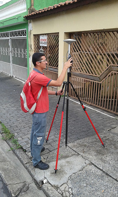
    The land surveyor and his or her staff use GPS daily, with varying degrees of accuracy. Here are a few examples:

    Mapping-Grade GPS Device (>= 3 meters)

    This handheld unit is primarily used for mapping utilities and improvements that don’t require high accuracy. The data and attributes acquired by this unit will be inserted into geographic information system (GIS) databases for inventory, and maintenance logs for future review and upgrade needs. Surveyors use these units for mapping items that require additional attributes and information necessary to improve the overall usefulness of a GIS database.

    Differential GPS (<= 1 meter)

    Differential GPS provides live positional solutions for applications that require more accuracy than mapping-grade GPS, at a reasonable equipment and operational price. These systems are used by aeronautical companies for mapping assistance, logistics companies for asset tracking, and emergency operations for 911 systems. These systems are also used by hydrographic surveyors for use in mapping lake and river bottoms as well as surveyors working in open pit mines, producing existing condition maps and volumetric surveys.

    Survey-Grade GPS

    Surveyors began implementing GPS equipment into their measuring repertoire in the mid 1980s with the introduction of data collection by static methods. This technique allowed for long-distance measurements with good accuracy and precision, but it came at an incredibly expensive cost.

    By the mid 1990s, real-time kinematic (RTK) equipment was introduced, and gave the land surveyor a new gateway into long-distance measurement with shorter occupation time and less cost. Additional enhancements to RTK systems included on-the-fly initialization, increased data-collector capability, and cellular/long-distance radio networks.

    These improvements allowed increased data-collection productivity, including mobile collection on all-terrain and survey vehicles. A topographic survey of a 40-acre parcel that would take several days of walking now is completed in less than 6 hours on an ATV. Boundary retracements of large parcels that used to take weeks of traversing the perimeter can now be done in a few days.

    Many credit GPS technology and functionality for greatly improving land surveying production as well as increasing accuracy and precision of the work.

    The Farmer

    Photo credit: ViaMoi via Foter.com / CC BY-NC-ND
    Photo credit: ViaMoi via Foter.com / CC BY-NC-ND

    Farming has been passed down from generation to generation for hundreds of years. History tells us this has been a hard life for many of these families as manual labor was at the root of the occupation. Livestock and family members were used to pull the necessary implements for planting each year’s crop, with most harvesting being done by hand.

    The Industrial Revolution brought the tractor and planting and harvesting equipment. After World War II, equipment manufacturers retooled their factories to increase the size and capacity of tractors. Even with the reduced manual labor that a farm tractor allowed, it was still a physical burden on the farmer planting crops and driving the miles of rows necessary to plant fields.

    Also, many agricultural areas became more organized, with local farm bureaus and associations being formed to help the farmer. These organizations provided information on how to increase yields in their crops; this data became the basic form of a GIS database for soils and drainage mapping well before digital mapping. These databases provided the initiative for the farmer to analyze planting methods and rates; herbicide, pesticide and fertilizer applications; and to review crop yields for notable increases and deficiencies.

    In the 1980s, yield monitoring equipment became a new tool for the forward-thinking farmer to invest in, analyzing how well his crops were producing. The only negative was the inability to accurately map the location of the various yield rates that would occur in the harvest. The farmer was forced to spend more time reading the yield analyzations in smaller parts of his fields in order to identify where adjustments were needed for increasing the output. Many farmers didn’t see the return on investment for this system, and those who did purchase such a system soon gave up.

    In the early 1990s, Rockwell International debuted the Vision System, a GPS unit using a U.S. Coast Guard correction system paired with a yield monitoring unit to map the location of yield rates during field operations. Trimble, John Deere and others were soon developing their own systems. All of these systems were expensive, delicate and too complex for most farmers to justify installing in their tractors.

    However, new discoveries in GPS technology during the late 1990s brought sweeping changes to this new tool for the farmer. While the term “precision agriculture” had floated around for a while, it wasn’t until the introduction of high-accuracy GPS that the statement reflected correctly on the industry.

    Differential GPS (<= 1 meter)

    John Deere began its pursuit of GPS technology in the early 1990s along with many others, but the company’s decision to continue pursuing this competitive edge is what led to several advancements for the farming industry. Deere’s work with Stanford University and NASA led to the revision of differential corrections for GPS locations to gain additional accuracy for a guidance system for Deere equipment.

    By 1998, John Deere presented a differential GPS system that provided 1-2 meter accuracy to assist farmers with smaller tolerances of precision field planting and harvesting. Innovations such as this led to many more advancements in the farming industry.

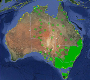
    Real-Time Kinematic (<= 2.5 centimeters)

    Today’s precision farming is more accurate than ever, with RTK networks providing a bulk of the coverage necessary to supply the farmer with corrections. In places where a local correction provider is not available, the farmer has choices of setting up his own base for correction or subscribing to other real-time networks via cellphone coverage. These systems allow for highly accurate mapping and guidance systems so the farmer has more control and information on his field and crops than ever before. Farmers now using GPS control in precise methods have more tools for increasing yields and production, including crop planning, soil sampling, pesticide/herbicide/fertilizer application and harvest analyzation.

    Crop planning used to be strictly in the hands of the farmer who drove his tractor in his field in an effort to follow the lay of the land. Today’s farmer uses topographic maps, aerial photography and mapping software to create planting patterns that make farming more efficient. By maximizing the planting configuration, this is also an opportunity to minimize fuel consumption. Soil sampling and weed mapping are now staples of many farmers’ activities.

    The farmer uses these methods to reduce the number of contaminants within the crop. He can also analyze the field’s health in order to apply the appropriate amount of necessary chemicals. These procedures are now computer controlled to vary the rate of application depending on the location within the field.

    Harvest analyzation has become the biggest source of data collected. Yield monitoring equipment was the first tool introduced into the electronic farming age. Now, coupled with GPS mapping of yield rates and volumes, farmers can accurately predict spot, regional and overall crop production from their fields. This data, along with soil mapping, is reviewed after the harvest and is used to determine a strategic plan for the next year’s planting.

    The biggest improvement, in most farmers’ opinions, is the implementation of steering-guidance systems. Initially produced to be strictly a guide to the driver, systems are now automated into the steering system to follow a predetermined path within a 1-inch tolerance. This frees the driver to monitor planting, spray application and harvesting operations.

    By turning the driving over to an automated system, field row overlap is reduced by up to 30 percent. This decreases double coverage of seed and spray application and it minimizes fuel consumption. This system also allows for less driver fatigue with the ability to work around the clock as needed or conditions dictate. Coupling this steering system with variable rate planters and sprayers, the farmer has a system that allows him to be more effective in managing and monitoring operations.

    Bringing the Two Occupations Together

    Both of these noble professions are using a highly accurate form of measurement and data recording, but we must review further how they can help each other. To do that, we must analyze what each is doing with the technology.

    Surveyors and GPS Use

    Roles of the surveyor are to measure land, provide his professional knowledge regarding parcel boundaries, and collect data for engineering and drainage purposes. A majority of this data is now collected by GPS methods and is in NAD83 state plane coordinates with NAVD88 elevations. This information can be supplemented by county and state GIS data as well. Surveyors also have knowledge of existing monuments by local, state and federal authorities tied to these coordinate systems/datums so all future surveys can be related to each other geographically.

    Farmers and GPS Use

    Farmers who have embraced GPS technology now have the power not only to map and collect data, but to also utilize previous data for crop efficiency. This ability to run a more efficient farming system is happening now for many farmers. The farmer is educated in regard to seed germination, weed and bug prevention, and maximizing crop yields so collecting this data has become a necessary task.

    The Farmer and the Surveyor — Harvesting Data

    The farmer and the surveyor can use their knowledge in many ways for the mutual benefit of increasing crop yields, efficiently working the land, and maximizing production.

    The surveyor’s knowledge of topography and drainage can assist the farmer with shaping of land to minimize water runoff and loss of key nutrients in the soil. This loss is estimated to be an average of two to three tons of soil per acre per year. Installation of drainage tile in addition to grading can be a critical part of minimizing soil loss, and the surveyor can help with this analysis.

    Accurate boundaries allow the farmer to know the limits of his property. The surveyor can provide this information so the farmer can maximize his planting configuration, yet not encroach on the adjacent property. The surveyor can also help with the creation of land-management systems to help farmland owners plan for financial decisions and tax strategies.

    The biggest opportunity for the surveyor is to offer assistance to the farmer who has little or no knowledge of data collection. This geospatial data can be confusing to those not familiar with this information. Farmers who become educated in analyzing and reading crop data can increase production and yields.

    Surveyors have the math skills and background to assist with the management of the data from a location standpoint. This effort will help the farmer know soil conditions, germination, spray application and harvesting to maximize the cost effectiveness of his investment in the land.

    Together, the farmer and the surveyor can create a successful partnership that can increase crop production worldwide. Data is the crop that brings them together, and planted with the right amount of care and nurturing, this data can become more valuable than ever.

  • NovAtel Showcases FlexPak6, FlexPak-S Receivers

    At Unmanned Systems 2015, held May 4-7 in Atlanta, NovAtel’s Peter Soar talks about the company’s FlexPak6 receiver that houses its OEM628 triple-frequency plus L-Band GNSS receiver board. It has a highly configurable interface to ensure precise positioning for UAV (unmanned aerial vehicle) applications. Soar explains that its “sister unit,” the FlexPak-S, contains a real time kinematic (RTK) GPS receiver with an L-3 XFACTOR Selective Availability Anti Spoofing Module (SAASM). The two receivers are both the same size and fit.

  • Latin America Sanitation Company Goes with ProMark

    Photo: Saneamento Basico do Estado de São Paulo (SABESP)Saneamento Basico do Estado de São Paulo (SABESP), a Brazilian water and sewage collection utility owned by São Paulo state and Latin America’s largest water company by market capitalization, has selected Spectra Precision ProMark 120 and 220 GNSS receivers to assist in gathering the geographic location of all SABESP network assets and the location of all customers.

    SABESP provides water to more than 28.7 million customers, or 67 percent of the population of São Paulo state. Water loss due to leakage in the SABESP network is a significant problem. The biggest reason behind water loss is leaks in the network; additional factors include sub-metering, caused by low water pressure; unauthorized consumption; and fraud. 

    Improving water management, recovering lost revenue and improving the quality of the customer experience is a priority for SABESP, Spectra Precision said. To help improve revenue generation and reduce water loss, SABESP developed two projects: LigGeo, to geo-reference the water meter location of approximately 4.8 million SABESP customers; and CadGeo, to geo-reference and register the location of the SABESP water and sewage network infrastructure.

    According to Marcos Almir, sanitation systems analyst for the metropolitan department of development and management of SABESP, the twin projects of LigGeo and CadGeo were motivated by SABESP’s desire to improve productivity and competitiveness. “We created an innovative GIS effort to geo-reference and register SABESP distribution networks and buried assets. Tests showed the technical feasibility of using ProMark GNSS receivers and collectors with NTRIP technology to efficiently and effectively register all SABESP equipment in real time with geo-referenced attributes connected to the technical and commercial enterprise systems to optimize processes and reduce costs.”

    To implement the LigGeo and CadGeo projects, SABESP purchased 50 ProMark 120 and 220 GNSS receivers from Hezolinem Equipamentos Topograficos, Spectra Precision’s Brazil dealer. Both SABESP technicians and outsourced service providers will use the receivers.

    ProMark 120/220 GNSS receivers were chosen for their multiple advantages: They could be purchased as rovers only; they could run LigGeo and CadGeo proprietary software; they are compatible with local third-party networks, including CEGAT, Brazil’s largest private RTK geodetic base network, that delivers RTK network corrections enabling real-time accuracy of less that 20 cm; and they offered direct two-way 3G communication of information with the SABESP central cartographic base raster files.


  • SuperPad GIS App to Receive NTRIP Solution

    SuperPad_NTRIPGIS software provider Supergeo will release an NTRIP solution on SuperPad, its Windows Mobile GIS app, for high-accuracy field data collection and geospatial workflow enhancement.

    SuperPad is a feature-rich mobile GIS application for field-based personnel to collect, edit, display and measure spatial data. The flexible development environment and customized extensions enable users to create a custom platform. SuperPad supports synchronizing data with an enterprise’s server to improve efficiency.

    SuperPad version 3.3 will support an NTRIP solution with RTK technology. Real-time kinematic (RTK) satellite navigation, one of the latest and widely used technologies within the field of differential GNSS, significantly enhances the precision of the positioning data. RTK positioning can raise accuracy to the centimeter-level.

    With the NTRIP solution, SuperPad is not only be capable of handling post-process DGNSS workflow, but also allows users to connect to network RTK service providers with NTRIP protocol, such as a virtual reference station RTK service provider or private station services. Its operations for turning on the module and quick-to-use settings will save surveyors time, while supporting GNSS receivers from makers such as  u-blox, Hemisphere GNSS and NovAtel.

    Progress of the SuperPad NTRIP Extension is also visualized as a condition monitoring informer on the map intuitively. Users looking for high accuracy or precision status with the RTK correction will find more details about the fixing mode and GNSS information presented clearly with the renewed GPS Status pages.

    A free trial of SuperPad can be downloaded here. A webinar about SuperPad is available here.

  • Trimble VRS Now Service Available in Australia, Oregon

    Trimble VRS Now Service Available in Australia, Oregon

    Trimble VRS Now coverage in Australia. Photo: Trimble
    Trimble VRS Now coverage in Australia. Photo: Trimble

    Trimble, together with its distribution partner Ultimate Positioning Group, announced the availability of Trimble VRS Now correction service in Queensland, New South Wales, South Australia, Tasmania and Victoria.

    Trimble is also now offering the Trimble VRS Now correction service in Oregon’s Willamette Valley.

    The commercial subscription service provides surveyors, civil engineers, geospatial professionals and other industry specialists in these areas with instant access to real-time kinematic (RTK) GNSS corrections without the need for a base station.

    Using both GPS and GLONASS constellations, the Trimble service delivers centimeter-level RTK corrections customized for each GNSS receiver’s location anywhere in the network via cellular communications. The Trimble VRS Now service supplies accurate, reliable and easy-to-use GNSS positioning for a variety of applications including surveying, urban planning, urban and rural construction, environmental monitoring, resource and territory management, disaster prevention and relief and scientific research, Trimble said.

    “The addition of VRS Now to Trimble’s current portfolio of corrections technologies and services in Australia highlights our ability to meet any accuracy, delivery, availability and financial consideration across a variety of applications and markets,” said John Sprivulis, business area director of Trimble’s Positioning Services Division in the Asia Pacific. “Trimble is effectively creating a national positioning infrastructure to meet Australia’s future needs.”

    Trimble VRS Now in Australia is a continuation of Trimble’s focus on providing solutions that enable customers to increase productivity by simplifying access to high-precision accuracy around the world. Similar VRS Now services are operating in parts of the U.S. and Europe.

    In addition, the Australian VRS Now service supports the Trimble Pivot Field Mobile App, which provides up-to-the-minute information on the VRS Now system status for users in the region.

    Because OmniSTAR CORS service in the area is being phased out, existing Australian users will be automatically transitioned to the Trimble VRS Now service, which provides easy access to high accuracy and reliable positioning within the network coverage area.

    Service in Australia and Oregon is a continuation of Trimble’s focus on providing solutions that enable customers to increase productivity by simplifying access to high-precision positioning around the world. Similar VRS Now services are operating in Illinois, Indiana, Iowa, Nebraska, Colorado, Florida, Alabama, Mississippi, Texas, and parts of Europe.

  • Leica Releases Viva GNSS Unlimited Series

    Leica Releases Viva GNSS Unlimited Series

    Leica_Viva_GS100-W
    Leica Viva GS100

    The Leica Viva GNSS Unlimited Series, available in August, will allow customers to make a safe investment with future-proof GNSS receivers and smart antennas, Leica Geosystems said in announcing the new series. With a flexible design, the Viva GNSS sensors can be upgraded for maximum performance whenever needed.

    The Leica Viva GNSS range fully supports the Chinese BeiDou navigation system. It can even provide BeiDou-only and GLONASS-only high-precision positioning. The unlimited series includes a future upgrade to a GNSS board with more than 500 channels and will serve users’ needs beyond 2020, the company said. Outages of real-time kinematic (RTK) communication links are bridged for up to 10 minutes with SmartLink to increase centimeter position availability in areas where RTK communications links are unstable.

    Leica Viva GS15
    Leica Viva GS15

    The Leica Viva GNSS Unlimited Series can be upgraded to the full range of GNSS signals. The sensors’ future-proof design is equipped for GNSS modernization, providing users with confidence in their investment. The series embraces the future-proof concept by including an upgrade to a GNSS board with more than 500 channels. To fully guarantee future proof GNSS, board exchanges are inevitable because any likely modifications in GNSS signals require a new GNSS ASIC (Application Specific Integrated Circuit).

    Leica SmartTrack technology guarantees accurate signal tracking, while SmartCheck technology evaluates and verifies RTK measurements to ensure reliable results. Both SmartTrack and SmartCheck technologies have been extended to support the BeiDou GNSS. BeiDou reached full operational regional capability in 2012 and has a total of 14 satellites. Leica Viva GNSS also supports features like BeiDou-only and GLONASS-only positioning to accommodate governmental regulations.

    In addition, Leica Geosystems now offers SmartLink, a correction service delivered via satellite for uninterrupted centimeter positioning in areas where RTK communication links are unstable.

    Leica Viva GS14
    Leica Viva GS14

    All Leica Viva GNSS products exceed the toughest environmental specifications, going beyond industrial standards such as IP68. This ensures flawless performance even in the most challenging environments. Applications for the range include construction and field surveying, mining, seismic work in dense forest, desert or mountains, as well as demanding work in extreme heat at 65°C (149 °F) or at extreme latitudes at -30°C (-22 °F). Premium precision and attention to detail ensure that the Leica Viva GNSS products can be trusted throughout the complete product lifetime.

    Leica Viva offers a complete range of unlimited GNSS and TPS solutions made with Swiss precision, combining the highest accuracy with maximum versatility and optimized data flow. Leica Viva solutions include Active Customer Care (ACC) with an expansive organization of knowledgeable professionals to provide valuable support, training and service whenever needed. Combined with innovative services such as online support in the field with Leica Active Assist and an instant data exchange between field and office with Leica Exchange, Leica Viva enables continuous productivity.


    Webinar on Multi-GNSS OEM

    Thursday, June 5
    10 a.m. PT / 1 p.m. ET / 5 p.m. GMT

    GPS World’s upcoming webinar features an expert panel with informed viewpoints from GNSS high-precision and mass-market manufacturing, signal simulation, and alternative PNT providers. Registration is free.

  • Centimeter-Level RTK Accuracy More and More Available — for Less and Less

    Eric Gakstatter
    Eric Gakstatter

    Last month, I started off 2014 with a bang by listing all the public RTK bases available in the United States, most of them being free. I received a lot of positive feedback and some enlightenment. For example, I didn’t know that in California, there are more than 330 RTK public base stations accessible by anyone for free via the California Real Time Network website at the University of California at San Diego! What a tremendous resource for California surveyors and GISers.

    Remember that RTK will give you 1-2 cm accuracy horizontally and twice that for vertical. If you know that and also know that there are 330 free RTK bases in California, why would anyone use post-processing for high-precision (e.g., sub-foot) GIS data collection? RTK technology used to be reserved for people who could spend tens of thousands of dollars on a GNSS receiver. Not any longer. RTK receivers are available for under $7,000, and you don’t need to invest in a RTK base unit if you’re in range of a public one on my list (or a commercial one not on my list).

    I’m pretty sure it was Charlie Trimble (founder of Trimble Navigation) who said “accuracy is addictive.” It sure is. Once you experience real-time centimeter-level accuracy (RTK) in the field, you won’t be satisfied with anything less, and neither will your GIS.

    I’ll keep updating the List of Public RTK Base Stations in the U.S. as people continue to inform me of ones that aren’t on my list. If you know of one, please email me.

    Keeping on the subject of RTK, 2014 might be the year of inexpensive RTK receivers. Whereas today you can find L1/L2 GNSS RTK receivers (in the U.S.) ranging from US$6,500 to US$25,000, there are rumors that some manufacturers are going to break through the US$6,500 price point.

    This is in line with the prediction I made a few years ago, but for a different reason. In 2010, I wrote that RTK receivers would become very inexpensive due to the new L5 signal being introduced, which would increase competition among GNSS receiver designers. I speculated that with more competition, the selling prices would significantly decline. Well, we are still without a usable L5 signal (although making progress) due to the slow deployment of modernized GPS satellites and the delay in Europe’s Galileo system, but we are still seeing a steady decline in the price of RTK receivers. Why is this?

    Even though there are a limited number of designers of RTK GNSS receivers, an increasing number of companies are buying RTK GNSS boards from these designers and making their own finished RTK GNSS receivers that look and perform very similar to receivers available today, for a fraction of the price. This is especially true in China, where there are several manufacturers buying RTK GNSS receiver boards from Trimble, Novatel, Hemisphere et al, making their own finished products and selling them. They were initially selling to very price-sensitive markets such as Africa, but now you see them setting up distribution in North America.

    This “OEM Syndrome” has put tremendous price pressure on existing brand-name RTK GNSS receivers as the Chinese-equivalent products are priced as little as 25% of the equivalent brand-name products. Of course, this drives the leading brand-name companies crazy. They are forced to either drop their price or otherwise convince buyers that their products are worth a significant premium. During these times of tight capital budgets, it’s increasingly difficult to do the latter. When enough satellites are in orbit broadcasting the L5 signal, you’ll really see this effect gain traction because there will be a lot more RTK GNSS designs to choose from, and the result will be better quality. More competition always results in better product quality and performance.

    The fact is that RTK receivers are moving towards becoming a commodity. As much as your local salesperson would like you to think they are selling a better RTK GNSS receiver, the technology gap between leading-brand designers and others is closing and probably unnoticeable to most of you. The major differences end up being the quality and reliability of the finished product (system design, battery, display, antenna integration, power supply, etc.). Having a great RTK GNSS receiver board inside is useless if the system design is unreliable.

    More Real-time PPP Competition

    For the longest time, it’s only been OmniStar (now owned by Trimble) and Starfire (owned by Deere & Co.) in the L-band high-precision correction game. Then, last year, the International GNSS Service announced its free decimeter real-time PPP service.  The catch is that receiver designers must incorporate IGS firmware to make use of the signal and…it’s only an Internet-based service (no satellite communications).

    In the past couple of months, Hexagon (which owns both Leica and Novatel), made a bid for Veripos. Veripos operates an L-band GNSS correction service for the oil and gas industry. Last year, TerraStar, a subsidiary of Veripos, announced its new decimeter service that is very similar to OmniStar and Starfire. It uses satellite communications for a data link. Altus Positioning Systems incorporated the TerraStar service into its receivers. Hexagon is very close to closing the deal with Veripos and just last week announced a partnership with competitor Topcon Positioning Systems. The result is that Leica and Topcon both will start offering high-precision L-band GNSS correction services with their receivers. If you’re an L-band decimeter user, this is probably good news for you. More competition = higher quality and lower price.

    Thanks, and see you next month.

    Follow me on Twitter at https://twitter.com/GPSGIS_Eric

  • Finally, a list of public RTK base stations in the US

    First of all, let me wish a Happy New Year to all my friends around the world and a prosperous 2014. I’m as excited as I’ve ever been about GNSS technology.

    If I may ask for forgiveness from you if you live outside of the United States, I’d like to start out answering a question I’ve been asked about for several years. The question is:

    Do you have a list of free sources of RTK base station data in the United States?

    What is RTK? In a nutshell, RTK is 1-2cm real-time positioning. Some refer to it as “survey-grade”. Historically, RTK users have been required to setup and maintain their own RTK base station. This is expensive and inconvenient. Many federal, state and local government agencies have setup RTK bases to increase RTK efficiency for their employees. Many of them make the RTK base data available to the public for free or for a nominal cost. If you work in an area that offers one, all you need is internet access in the field and a RTK-capable GPS L1/L2 receiver.

    I’ve tried to keep track of the public RTK bases I know of, so I’ll list them here. If I’ve missed one you know of, please feel free to send me a quick email at [email protected] or list it in the Comments section at the end of this article. Furthermore, if you live outside of the U.S., I’d love to hear from you if you know of a source of free RTK base data.

    Please note that in the following list there are four types of RTK bases:

    1. Trimble VRS (network solution).
    2. Leica Spider (network solution).
    3. Single baseline (eg. Plate Boundary Observatory  and CRTN).
    4. Topcon TopNet (network solution).

    I’ve used an RTK rover on all three of these services. Each of them has several mount points supporting different data formats. I typically use RTCM3 format because it’s an open standard and supported by all services I’ve used. For the Leica Spider network, you’ll be presented a choice of iMAX or MAX. Choose iMAX if you’re not running a Leica rover.

    To use any of the services, you’ll need Internet connectivity. In the past, I’ve accomplished this in a few ways:

    1. SIM card inside a data collector.
    2. MiFi device.
    3. Wi-Fi from a work vehicle.

    You can also use a commercial RTK Bridge or Repeater such as Intuicom or Base-n-ABox. Or you can create your own RTK bridge system with a notebook computer that has internet access.

    No matter how you do it, you’ll need a reliable Internet connection (speed is not important).

    You’ll also need some sort of NTRIP software utility. Several data collector software packages have this built-in. For software like ArcPad, DigiTerra, gvSIG, etc. that don’t have it built-in, there are some freeware utilities on the market that run on Windows and Windows Mobile and Android (for example, SXRTN or Lefebure) that handle the NTRIP tasks in the background.

    If you want to read a detailed article about the process of logging in to an RTK base using NTRIP, I wrote one last year while I was in Colorado. Click here to have a look. I also published another article entitled “Sources of Public Real-Time High-Precision Corrections” that you might be interested in.

    Following is a list of RTK bases in each U.S. state, along with the associated website. Please note that I only list the public (government-operated) services. Also note that while most are free, some of the public operators charge a user fee. At one point or another, I’ve used a fair number of these in various states. Once you’ve used one of each (Trimble, Leica, PBO), the rest are pretty much the same.

    The difference between the Trimble and Leica networks and PBO is that the Trimble and Leica networks provide a network solution that utilizes several RTK base stations in the computation. Distance-dependent errors are reasonably modeled so the user can be farther from individual RTK bases. The PBO RTK bases provide a single baseline (like everyone used to use before RTK networks were invented) so the further you are from the RTK base, the more error is introduced into the solution (roughly 1 cm + 1 ppm).

    Lastly, there are a number of commercial RTK networks in most of the states listed. I’ll save that list for another day. Again, these are just the publicly run RTK bases.

    Alabama – Alabama Department of Transportation. Leica network.

    Alaska – Two PBO RTK bases. One in Fairbanks and one in Palmer. Otherwise, no public service.

    Arizona – Arizona State Cartographer’s Office. Leica network. Plate Boundary Observatory (single baseline).

    Arkansas – No public service.

    California – California Real Time Nework (CRTN) (single baseline).  Plate Boundary Observatory. Single baseline.

    Colorado – Mesa County (Trimble network) and Plate Boundary Observatory (single baseline).

    Connecticut – No public service.

    Delaware – No public service.

    Florida – Florida Department of Transportation. Leica network.

    Georgia – No public service.

    Hawaii – No public service.

    Idaho – Plate Boundary Observatory (single baseline).

    Illinois – No public service.

    Indiana – Indiana Department of Transportation. Leica network.

    Iowa – Iowa Department of Transportation. Leica network.

    Kansas – No public service.

    Kentucky – Kentucky Transportation Cabinet. Trimble network.

    Louisiana – Louisiana State University. Trimble network.

    Maine – Maine Department of Transportation. Trimble network.

    Maryland – No public service.

    Massachusetts – Massachusetts Department of Transportation. Leica network.

    Michigan – Michigan Department of Transportation. Leica network.

    Minnesota – Department of Transportation. Trimble network.

    Mississippi – University of Southern Mississippi. Trimble network.

    Missouri – Missouri Department of Transportation. Trimble network.

    Montana – Plate Boundary Observatory (single baseline).

    Nebraska – No public service.

    Nevada – Washoe County. Trimble network. Las Vegas Valley Water District. Leica network.  Plate Boundary Observatory (single baseline).

    New Hampshire – No public service.

    New Jersey – No public service.

    New Mexico – Plate Boundary Observatory (single baseline).

    New York – New York Department of Transportation. Leica network.

    North Carolina – N.C. Department of Environment and Natural Resources. Trimble network. $500 one-time sign-up fee.

    North Dakota – No public service.

    Ohio – Ohio Department of Transportation. Trimble network.

    Oklahoma – No public service.

    Oregon – Oregon Department of Transportation. Leica network. Plate Boundary Observatory (single baseline).

    Pennsylvania – No public service.

    Rhode Island – No public service.

    South Carolina – South Carolina Geodetic Survey. Public but charges a usage fee. Trimble network.

    South Dakota – No public service.

    Tennessee – Tennessee Department of Transportation. Public but charges a usage fee. Topcon network.

    Texas – Texas Department of Transportation. Public but only available to TxDOT employees and TxDOT contractors. Trimble network.

    Utah – Utah Automated Geographic Reference Center.  Public but charges a usage fee. Trimble network. Plate Boundary Observatory (single baseline).

    Vermont – Vermont Geodetic Survey. Trimble network.

    Virginia – No public service.

    Washington – Washington State Reference Network (Seattle Public Utilities). Trimble network. Public but charges a usage fee. Pierce County (Leica Network). Plate Boundary Observatory (single baseline).

    West Virginia – West Virginia Department of Transportation. Trimble network.

    Wisconsin – Wisconsin Department of Transportation. Trimble network.

    Wyoming – Plate Boundary Observatory (single baseline).

    Thanks, and see you next time.

    Follow me on Twitter at https://twitter.com/GPSGIS_Eric

  • Network RTK for Intelligent Vehicles

    opener

    Accurate, Reliable, Available, Continuous Positioning for Cooperative Driving

    By Scott Stephenson, Xiaolin Meng, Terry Moore, Anthony Baxendale, and Tim Edwards

    Adoption of network real-time kinematic GNSS positioning can lead to major improvements in vehicle localization, although implementation must overcome some real-world challenges. This article assesses the extent of GNSS signal outage in a motorway environment. The average total GNSS outage period and the average time to resolve ambiguity for the network RTK solution can help assess complimentary sensors for a ubiquitous positioning system.

    Real-time vehicle localization is one of three key enabling technologies for the concepts of vehicle-to-vehicle and vehicle-to-infrastructure (V2V and V2I, collectively termed V2X, see opening graphic), a classification of intelligent transport systems (ITS). The further enabling technologies are ad-hoc dynamic networking of agents, and accurate dynamic local traffic maps. Jointly, these require that positioning be accurate, reliable, available, and continuous.

    A natural evolution in road transport, V2X promises to deliver the next major safety breakthrough. The concept moves away from vehicles making individual decisions about road safety, as in advanced driver assistance systems, and towards a cooperative driving approach that shifts the emphasis from collision protection to collision prevention. The U.S. National Highway Traffic Safety Administration  estimates that V2X technology can avoid or minimize up to 80 percent of collisions of unimpaired drivers, and that even a small number of deployed vehicles will provide tangible safety benefits.

    Network RTK GNSS positioning, like V2X applications, requires a communication system; and by its nature V2X has a positioning solution requirement. Thus it is envisioned that network RTK will play an essential role in the implementation of V2X systems. The consensus between car manufacturers and research organizations is that the future of V2X communication lies with Dedicated Short Range Communication (DSRC) devices, and a large pilot study is currently under way. However, in the short term many V2X applications could be achieved using existing technology, such as cellular communication, offering a legacy solution, and initiating early uptake of V2X applications.

    Previous research by the Nottingham Geospatial Institute (NGI) at the University of Nottingham showed that network RTK positioning can provide a high-accuracy positioning solution during real-world trials, but also revealed two areas of concern: the loss of the fixed-integer ambiguity during satellite line-of-sight outages; and the fragility of the data communications service that delivers the real-time correction information. During road tests, a fixed-ambiguity network RTK solution was available for less than 50 percent of the time on United Kingdom (UK) roads.

    Network RTK Vehicle Positioning
    Figure 1  OS Net reference station network in Britain, owned by Ordnance Survey.
    Figure 1. OS Net reference station network in Britain, owned by Ordnance Survey.

    Networks of continuously operating reference stations (CORS) extend across Europe, North America, Australia, and East Asia. Networks vary in size from five or six reference stations for agriculture to systems of hundreds of CORSs providing national or regional service. Figure 1 shows the location of the OS Net CORS run by Ordnance Survey in Great Britain.

    Figure 2 shows the main advantage of network RTK as compared to traditional RTK. The individual reference stations on the left suffer from the spatial decorrelation of errors as distance between reference and rover receivers increases. Adequate vehicle positioning would require individually operating reference stations to be placed approximately 20–30 kilometers apart. However, a CORS network can be used to develop a model of differential corrections, as shown at right, from which a rover receiver can interpret RTK correction information and use this during the computation of its position. The geometry of a CORS network allows two adjacent reference stations to be located up to 80–100 kilometers apart without degrading the accuracy, although in practice most systems tend to locate them closer together than this. This is essentially a reduction from 30 reference stations per 10,000km² for conventional RTK, to 5–10 reference stations for network RTK, delivering high-precision services to virtually unlimited users.

    Figure 2  The improved navigation performance from RTK (left) to network RTK (right).
    Figure 2. The improved navigation performance from RTK (left) to network RTK (right).

    It is expected that the CORS networks will become a critical part of a country’s spatial infrastructure, and countries like the UK are leading the way. This makes network RTK one of the most promising positioning technologies for road vehicles and ITS applications.

    As shown in previous research, network RTK can deliver a vehicle positioning accuracy of better than 5 centimeters, and in real-world tests this level of accuracy had an availability of 41–45 percent, depending on the environment. It was also found that the correction information was available via the GSM network for more than 80 percent of the time. In these same tests, the total time without any GNSS position solution (network RTK, DGNSS, or stand-alone) was up to 16 percent in a motorway environment. Network RTK was able to provide lane-level positioning accuracy, but the sensitivity of the technique to GNSS signal loss and coverage of the communication network had a significant effect on availability. GNSS outages could be caused simply by passing under a road bridge, and the network RTK solution would be lost, although there would continue to be a DGNSS solution for a short period. Finding effective solutions to these current barriers, which prevent wide adoption of network RTK, is a key enabling step for ITS.

    Accuracy Assessment

    In much more controlled tests to assess the accuracy of network RTK on a dynamic vehicle, the network RTK GNSS receiver was compared to an inertial navigation system (INS). This test was carried out using the NGI roof laboratory, which houses a 120-meter rail track running an electric locomotive.

    Both the network RTK receiver and the INS used the same antenna, fed separately through a signal splitter. The network RTK solution was recorded in real time onto an SD card in NMEA GGA format. The INS data was recorded and post-processed in a tightly coupled solution using a continuously operating dual-frequency GNSS receiver base station located inside the rail track circuit. There were no recorded GNSS outages as there is a clear-sky view from the roof laboratory.

    The antenna point was also tracked using a total station, recording observations at 10 Hz stamped with GPS time. Although the accuracy of the tracking mode of the total station is not high enough to assess the accuracy of the network RTK solution (because of time synchronization issues), it ensures that any gross errors in GNSS observations that could affect both the network RTK and INS solutions did not occur.

    The results in Table 1 show that the network RTK solution consistently performs to a high accuracy, giving a low standard deviation from the mean in all directions. Listed are three laps of the rail circuit recorded at different times. There are a small number of epochs that encounter large differences of more than 200 millimeters, such as during laps 2 and 3, although these appear to be very short-term anomalies, possibly caused by dynamic GNSS signal multipath or delays and message loss in the communication system.

    TABLE 1.  Comparison of the tightly coupled (GPS+IMU) solution with the N-RTK solution.
    Table 1. Comparison of the tightly coupled (GPS+IMU) solution with the N-RTK solution.

    The worst absolute accuracy is shown during lap 3, although even in this case, with a mean of 21 millimeters and 99 percent of the observations lying within 15 millimeters, this solution still delivers a solution within 36 millimeters of the ground truth. 50 percent of the network RTK observations are within 1 millimeter of the mean difference between the two solutions, showing remarkable consistency and precision.

    Challenge: Comm Signal Strength

    A fundamental aspect of network RTK is the delivery of reference station data used in the processing of the receiver’s position. Although there are various methods used to deliver this data, the most secure and reliable method involves transmitting raw reference station observations, so that the receiver may perform the calculation of the position with all possible data. This provides the highest integrity. The vulnerability here is not the algorithmic method used to transmit the data, but the communication system, in three ways:

    • There is no connection between reference and rover receivers.
    • There is data loss from the connection.
    • There is an unacceptable delay in the transmission of the data.

    Lack of Coverage. The preferable communication system is to use mobile Internet over the GSM/GPRS cell network, which is already well established. The major network operators claim over 99 percent coverage of the population in the UK, but this does not take into account physical and local conditions such as land and building obstructions, atmospheric conditions, and inter-ference from vegetation and other
    radio signals.

    A 2011 BBC survey in the UK found that when users had a cell-phone data connection it was 3G for 75 percent of the time (2G otherwise), but significant “notspots” include major rail and road networks. An ongoing study by OpenSignalMaps has found that a 3G service is only available 58 percent of the time. A 2011 government report detailed the extent of 2G and 3G services, shown in Figure 3. Areas with poor data communication coverage (below 50 percent) pose a significant problem for network RTK in vehicles.

    Figure 3 2G (left) and 3G (right) coverage by geographic area in the UK: green, >90 percent; yellow, 70–90 percent; blue, 50–70 percent; purple, 25–50 percent; red, <25 percent.
    Figure 3. 2G (left) and 3G (right) coverage by geographic area in the UK: green, >90 percent; yellow, 70–90 percent; blue, 50–70 percent; purple, 25–50 percent; red,

    Data Loss. Continuity tests show that when using GSM/GPRS mobile communications to transfer the network  RTK corrections, the availability was approximately 88 percent, and the connection could be lost after a few hours of continuous use. This can be caused either by SIM cards that use dynamic IP addresses, creating interruptions when renewing the addresses, or where voice data was prioritized on the network. Other research has shown that a typical mobile Internet connection (a combination of wired public Internet and GPRS) suffers from approximately 20 percent data loss.

    Message Delay. A network RTK receiver  imposes a transmission time limit on the correction messages that are used to fix the common integer ambiguity (in this case, the Leica GS10 limit is 10 seconds), although messages younger than 60 seconds can be used to give an accurate DGNSS solution. Messages older than 60 seconds result in the receiver only being able to output a standalone position, by which time the accuracy will decay beyond vehicle positioning requirements. Earlier research found the typical mobile Internet connection suffers from an average delay of 0.85 seconds.

    Challenge: GNSS Outages

    The majority of the transport infrastructure is outside and has a clear view of the sky, particularly away from heavily urbanised areas. However, the receiver gets no warning of impending signal obstruction, so that even momentary obstructions such as an overhead gantry on the motorway can cause significant loss of positioning accuracy, and often causes a receiver to output no solution at all, as shown in Figure 4. Here the vehicle is traveling in a northern direction in lane 1 of the left-hand carriageway and passes underneath a series of bridges at a motorway junction. This causes both GNSS outages and deteriorated positional accuracy, so much so that the vehicle is positioned in the southern carriageway (note that the underlying map image is of unknown accuracy).

    Figure 4  The typical effect of overhead obstructions on vehicle GNSS positioning.
    Figure 4. The typical effect of overhead obstructions on vehicle GNSS positioning.

    GNSS outages can occur in several ways: the obstruction of the GNSS signals can lead to a loss of signal lock; a momentary obstruction or partial obstruction can cause cycle slips to occur (during carrier-phase positioning); if the visible satellites at the rover receiver are not the same as at the reference receiver, then the ambiguity cannot be resolved; there may be intentional or unintentional signal jamming or interference; and if the receiver assessed the integrity or accuracy to be poor then it may not provide a solution.

    NGI test vehicle.
    NGI test vehicle.
    Experiment Set-Up

    The test vehicle was equipped with a GNSS receiver and antenna, receiving real-time corrections using a GSM/GPRS connection. The signal strength was measured simultaneously using the Android application RF Signal Tracker on an Android-based mobile phone.

    The data recorded includes: GNSS raw data, RINEX format; network RTK real time output, NMEA format; GSM signal strength, CSV format. As the experiments were not intended for the analysis of the accuracy of the GNSS receiver, there was no need to utilize the ground truth system onboard the NGI test vehicle.

    RF SIGNAL TRACKER Android application and mobile phone used to record the GSM signal strength (left), and GNSS receiver (right).
    RF SIGNAL TRACKER. Android application and mobile phone used to record the GSM signal strength (left), and GNSS receiver (right).

    Test Environment. Two test scenarios were chosen for the experiments. To assess the GNSS signal outages, the test vehicle was driven along the M1 motorway, a length of approximately 100 kilometers. The M1 is a major road transport artery linking London in the South to Leeds in the North of England, typically with three or four lanes in each direction. This route passes under 214 overhead obstructions (northbound and southbound directions), of known classification (gantry, footbridge, road bridge). This scenario was chosen as the environment is quite rigid, allowing repeatable tests, and it is the area in which future ITS technology is most likely to be adopted first.

    To test the variation of GSM signal strength in real-world conditions, a small circuit was chosen close to the Nottingham Geospatial Institute (shown in Figure 5), which incorporates a variety of environments from open sky to bridge underpasses, and dense tree coverage. Using a repeatable path allows the identification of issues that are attributable to problems with the communications link as opposed to other issues (such as hardware problems and GNSS signal outages), and despite the short distance, the loop also provides a wide range of GSM signal strengths. During the experiments to follow, the data was measured during three consecutive laps of the circuit.

    Experiment Results

    GSM Signal Strength. The variation in color along the NGI test route is an indication of the RSSI (Received Signal Strength Indicator). In this area, the RSSI varies between –50 dBm and –105 dBm, which are the typical maximum and minimum strengths of a cellular network. This is despite the assessment from the network provider that this entire area delivers high-speed Internet and email. Figure 5 also shows the subjective rating and expected performance of the RSSI.

    Figure 5  The GSM signal strength around the NGI circuit in Nottingham, with the subjective RSSI ratings.
    Figure 5. The GSM signal strength around the NGI circuit in Nottingham, with the subjective RSSI ratings.
    Table2
    Table 2. The spread of RSSI observations recorded during the trials around the NGI circuit.

    Table 2 details the RSSI observations measured during the signal strength trials around the NGI circuit. The range of values shows the typical maximum and minimum RSSI values experienced by a cell-phone user (other than no signal being received). The signal strength is recorded every 5 meters, in order to achieve a good geographic spread across the area (as opposed to biasing the results with observations recorded whilst the vehicle is stationary). The RSSI observations do not correspond to a typical Gaussian distribution, suggesting that there are external influences on the strength of the signal and the handover between one cell tower and the next.

    Figure 6 shows an increase in the age of correction (AoC) of the messages following a drop in signal strength (RSSI) to approximately –100 dBm. This is visible from the peaks in the age of correction message to over 8 seconds. The graph shows three laps of the NGI circuit, noticeable by the repeated pattern of signal strength. The increase in the AoC occurs at approximately the same geographic location on each lap ­— an area in the northwest of the circuit that suffers from weak signal strength, as seen in Figure 5. The received signal strength is the sum of the direct and indirect (or reflected) waves, varying with distance between a series of maximum and minimum values. On a moving vehicle, the RSSI will vary with time as it moves between these maximum and minimum values, and is especially complicated in urban areas where there may be no direct waves at all, and waves are propagated by a series of reflections. A moving receiver also suffers from a Doppler shift in the received signal’s frequency.

    figure 6  The effect of GSM RSSI on the age of correction messages.
    Figure 6. The effect of GSM RSSI on the age of correction messages.

    During network RTK positioning, the receiver considers messages older than 10 seconds unusable for a fixed network  RTK solution, although messages younger than 60 seconds can be used to give an accurate DGNSS solution. This scenario has a brief occasion during the loop in which loss of the network RTK solution is attributable to weak GSM signal strength.

    A close inspection of Figure 6 highlights a slight delay between the drop in RSSI to –100 dBm and the increase in the AoC. This delay needs further analysis, but is assumed to relate to the slower update rate of the ionospheric and tropospheric corrections (10 seconds and 60 seconds respectively). There are also periods of increased AoC that are uncorrelated with a drop in RSSI, for which there is no clear explanation, although none of these occasions results in a loss of the fixed ambiguity network RTK solution.

    Eighty cell handovers were recorded during the trials, which is higher than average as this area is liable to carry a large volume of cellular traffic (there is a university, a large hospital, and major roads, as well as general housing and business properties). The cell handovers showed an average improvement of +1.2 dBm from just before the handover until just after. The maximum improvement is +22 dBM, although there are occasions when the RSSI gets worse, the biggest fall in received signal strength being –12 dBM. Figure 7 displays the frequency distribution of the change in RSSI during a cell handover. The resolution of the RSSI measurements is 2 dBm.

    figure 7  Frequency histogram of the RSSI change during a cell handover (2 dBm bins).
    Figure 7. Frequency histogram of the RSSI change during a cell handover (2 dBm bins).

    Cell handovers occur at a range of RSSI, not just low signal strength. This suggests that cell handovers are managed by the network operator in a way that does not disrupt the data connection. There appears to be no correlation between a cell handover and a problem with the correction message delivery.
    Although this part of the experiment was not a test of receiver performance, during the NGI circuit trial 63.1 percent of the receiver observations were network RTK fixed, and 33.0 percent of the observations were DGNSS observations. Therefore, 3.9 percent of the possible epochs had no observations, partly due to passing under bridges. The largest GNSS outage during circuit trials was 4.85 seconds. These values show an improvement over previous research, particularly as this is considered a difficult GNSS positioning environment.

    GNSS Outages. During the GNSS outages tests, the vehicle traveled at a constant speed of 60 mph, mostly in lane 1 of the motorway. Table 3 shows statistical breakdown of the GNSS outages and the resulting reacquisition of the fixed ambiguity in network RTK positioning.

    Table3
    Table 3. Statistical breakdown of GNSS outages caused by overhead objects.

    The longest total GNSS outage caused by an overhead obstruction was 4.65 seconds, when passing under a road bridge. At 60 mph this translates into a distance of almost 130 meters without any GNSS solution, which is much further than the width of the overhead object. Once the GNSS signal is reacquired, there is a short period during which the fixed integer ambiguity is resolved, in order to achieve the centimeter-level accuracy. The longest duration between start of a GNSS outage and reacquisition of the fixed ambiguity for the network  RTK solution is 52.10 seconds, or 1,450 meters. Although during this period, a DGNSS solution is available as soon as the satellites are reacquired.

    Discussion

    Nationwide adoption of cellular Internet services by cell phone users has provided a useful communication system for positioning systems. But network providers do not guarantee the type of communication service demanded by advanced ITS and V2X applications. The quality of service is too easily disrupted by passing into an area with weak signal strength, or when many users congest the bandwidth.

    Future generations of cell networks, such as 4G, will significantly increase the available bandwidth and increase download speeds, but there is an unknown increase in the demand on the system from non-critical cell-phone users. The issues in the existing system can be minimized slightly through improvements at the user end, such as using stronger gain antennae or accessing multiple networks with different SIM registrations. The nature of cell networks also leads to a decrease in signal strength occurring prior to the cell handover, which can cause delays in the message delivery, so the management of this process could be improved. Future testing of the GSM network can be carried out at the new innovITS ADVANCE test facility at MIRA in the UK, where the private network can be controlled and manipulated as desired.

    An alternative communication method, that has the same wide area coverage of a cell network, is satellite communication. In tests, observation of static positions showed 98 percent of messages were received correctly at a latency of less than 10s. This compares with the High-Speed Download Packet Access (HSDPA) cell network figures of 99.8 percent and 1.2s. When in a kinematic mode, the satellite communications fared less well. Testing three separate satellite communication systems, problems were encountered with reacquisition, long latency, and static initialization. At best, 70 percent of correct messages were received, with a latency of 4.2s, although often over 20s.

    Digital Audio Broadcasting (DAB) is capable of being used as a future communication method for network  RTK positioning. Compared to traditional VHF and UHF radio communication, it uses the frequency more efficiently and is more robust to degradation.

    The design of the GNSS receiver used in testing is aimed at delivering a very reliable and highly accurate solution. It was not intended for use on vehicles and in dynamic environments. The receiver deals well with multipath, rejecting low-strength GNSS signals, allowing the resolution of the integer ambiguity. However, this means that in city environments it may provide fewer solutions than a modern smartphone, albeit with a much higher accuracy when it does. Recent research shows it is possible to increase the speed of ambiguity resolution, and customize integrity controls, making the resolution process close to instantaneous in certain circumstances.

    Conclusions

    As cellular communications networks evolve in the UK and other countries, the performance of the network  RTK receiver also improves. We found that once the RSSI drops to approximately –100dBm, the correction messages suffer from either message loss or message delay that causes the receiver to underperform. The performance of the communication link during a cell tower handover has shown that there is no deterioration in the performance linked to the handover, although cell tower handovers generally occur at the limits of a cell tower’s coverage, and hence at low signal strengths.

    The resolution of the fixed integer ambiguity is crucial for the high-accuracy solution available with a network RTK receiver. The resolution is relatively fast, typically within two minutes from a cold start, or fewer than 20 seconds from a hot start. During tests on the M1 motorway, passing under an overhead obstruction caused a maximum total GNSS outage of 4.65 seconds, and a maximum time until the ambiguity was resolved of 52.10 seconds. On average, the GNSS outage was 1.14 seconds with an average re-fix time of 13.13 seconds. Until the ambiguity is resolved, the receiver can continue with a DGNSS solution delivering lane-level accuracy.

    Manufacturers

    NGI’s inertial nav system is an Applanix POS/RS, which consists of a NovAtel OEM4 dual-frequency GPS receiver combined with a navigation-grade Honeywell consumer IMU. The network RTK position was provided by a Leica GS10 receiver and Leica SmartNet correction service over the Vodafone network. Both receivers used a Leica AS10 antenna.


    Scott Stephenson is a Ph.D. student at the Nottingham Geospatial Institute within the University of Nottingham.

    Xiaolin Meng is associate professor, theme leader for positioning and navigation technologies, and MSc course director for GNSST and PNT at the Nottingham Geospatial Institute of the University of Nottingham. 

    Terry Moore is director of the Nottingham Geospatial Institute (NGI) at the University of Nottingham, where he is the professor of satellite navigation and also an associate dean within the Faculty of Engineering.

    Anthony Baxendale is head of Advanced Technologies & Research at MIRA Ltd.

    Tim Edwards is the lead engineer of the Intelligent Transportation Systems (ITS) research group at MIRA Ltd

  • Leadership Awards 2012: Real-Time Kinematic in Your Palm

    Technology to Be Cheap and Pervasive by 2020


    Editor’s Note: This article reproduces the acceptance speeches given by the winners of GPS World’s 2012 Leadership Awards, at the Leadership Dinner in Nashville in September. The Leadership Dinner was sponsored by Lockheed Martin and Deimos Space.


    Remarks by Todd Humphreys, Radionavigation Laboratory (director), University of Texas at Austin (assistant professor), winner in the Signals category. He is the leader of several seminal studies on spoofing and jamming, and he testified this summer before Congress on the subject.


    It’s a genuine honor to receive this award. I’d like to thank Alan Cameron and all the contributors to GPS World. GPS World plays an essential role in building our GNSS community and keeping it together, providing GNSS news, instruction, and, indispensably, gossip!

    I’d also like to thank my students at the University of Texas Radionavigation Lab. Much of the credit for this award goes to them.

    The futurist Ray Kurzweil spoke at a conference I attended back in 2001. Maybe some of you have heard of Ray. He’s regarded variously as a prophet, or a crackpot. He’s taking hundreds of vitamins every day to keep himself alive until the singularity arrives, at which point he’ll download himself onto a robot and live forever, or at least he’ll have his head cryogenically frozen so that he can be downloaded and live forever later on.

    In that 2001 talk, Ray made some bold predictions. One, in particular, I remember well. “Within the decade,” Ray assured us, “we’ll all be wearing special contact lenses that give us a permanant Internet feed directly to our eyeballs.”

    Nonsense, I thought, and indeed it was nonsense. Here we are in 2012 and no such contact lenses exist, nevermind their being in widespread use.

    I resolved back then that if I were ever called on to peer into the future and tell what I see, as Alan has asked me to do tonight, I’d be more modest about it.

    So tonight I’m going to make a modest prediction, and only one of them. I predict that by the GPS World dinner in 2020, carrier-phase differential GNSS, or, if you prefer an adjective for what should be a noun, Real-Time Kinematic, will be cheap and pervasive. We’ll have it on our cell phones and our tablets. There will be app families devoted to decimeter- and centimeter-level accuracy. The consequences will be fantastic. And this will be enormously disruptive to the current precision navigation industry. This will be the commoditization of centimeter-level GNSS.

    Now you may very well object to this prediction. You might point out that integer ambiguities will be difficult to resolve in the face of the near-field effects around and poor placement of the GNSS antenna in handheld units. You might also argue that the increased power requirements of carrier-phase techniques will be a dealbreaker for mobile devices. That’s all fine. I agree that those are hard problems. My students and I are looking into them, trying to overcome them.

    But please don’t make as one of your objections the one that I’ve heard so many times: “Why would anyone ever want centimeter-accurate positioning in their cell phone?” Because I’ll object that your objection lacks imagination.

    To see one example of what could be done with commoditized centimeter-accurate GNSS, I invite you all to a presentation by my students Daniel Shepard, Ken Pesyna, and Jahshan Bhatti tomorrow in the F5 Session (Millimeter-accurate Augmented Reality Enabled by Carrier-Phase Differential GPS). They’ll show off a crude box that we’ve built, through which, if you peer, you can see a sandcastle that’s not really there. And you can walk around the sandcastle and see it from all sides with centimeter accuracy.

    Imagine when this technology is in our tablets! Or, better yet, when it’s in our glasses — or, I suppose, our contact lenses. Not that I’m making any predictions about contact lenses.

    [Ed. For a short video demonstration of the RTK-enabled augmented reality box built by Todd Humphreys’ students, visit this site.]

  • Real-Time Extended GNSS Positioning: A New Generation of Centimeter-Accurate Networks

    A new method brings together advantages of real-time kinematic (RTK) and precise point positioning (PPP) in a technique that does not require local reference stations, while still providing the the high productivity and accuracy of RTK systems with the extended coverage area of solutions based on global satellite corrections. The real-time centimeter-level accuracy without reference-station infrastructure is suitable for many market segments — and is applicable to multi-GNSS constellations.


    By Rodrigo Leandro, Herbert Landau, Markus Nitschke, Markus Glocker, Stephan Seeger, Xiaoming Chen, Alois Deking, Mohamed Ben Tahar, Feipeng Zhang, Kendall Ferguson, Ralf Stolz, Nick Talbot, Gang Lu, Timo Allison, Markus Brandl, Victor Gomez, Wei Cao, and Adrian Kipka

    Real-Time eXtended (RTX) positioning is a technology produced by combining a variety of innovative techniques, which together provide users with centimeter-level real-time position accuracy anywhere on or near the Earth’s surface. This new technique is based on the generation and delivery of precise satellite corrections (that is, orbit, clocks, and others) on a global scale, either through a satellite link or the Internet. The innovative aspects of the new solution can be divided into different categories, which directly relate to the areas that have previously limited the provision of global high-accuracy positioning:

    • Integer-level ambiguities derivation;
    • Real-time, high-accuracy satellite corrections generation;
    • Data transmission optimization;
    • Positioning technology.

    Because of various new aspects of the technique, RTX differs from both differential RTK and precise point positioning as currently understood by the general GNSS community.

    System Overview

    RTX technology is used to provide centimeter-level GNSS positioning through the CenterPoint RTX service. Figure 1 shows the general infrastructure of the system.


    Data from monitoring stations distributed around the globe are collected and transmitted via the Internet to operation centers at different locations. The complete operation centers (enclosed by the red dashed square) are redundant in order to assure the very high (~100 percent) availability of the system. In case it is needed, the correction stream source might change between operation centers and/or processing servers within centers. These operational changes are handled in a deterministic way by all parts of the system including the user receiver. Inside the operation centers, redundant communication servers relay the network observation data to the data processing servers, which host the network processors that produce precise orbit, clock, and observation biases valid for any place on the globe.

    After being generated, the precise satellite data are compressed in messages compliant with the CMRx format, specially developed for compact transmission of satellite information. The messages are finally routed to either a satellite uplink station or made available for Internet connection access by the users.

    The CenterPoint RTX tracking network currently consists of around 100 stations, distributed across the globe, as shown in Figure 2. The CenterPoint RTX service is currently offered in North and South America, via satellite link, as indicated in Figure 3. Today the CenterPoint RTX service has been made available globally for all those with Internet access.

    Photo: Rodrigo Leandro, Herbert Landau, Markus Nitschke, Markus Glocker, Stephan Seeger, Xiaoming Chen, Alois Deking, Mohamed Ben Tahar, Feipeng Zhang, Kendall Ferguson, Ralf Stolz, Nick Talbot, Gang Lu, Timo Allison, Markus Brandl, Victor Gomez, Wei Cao, and Adrian Kipka
    FIGURE 2. CenterPoint RTX tracking network distribution. (Click to enlarge.)
    Photo: Rodrigo Leandro, Herbert Landau, Markus Nitschke, Markus Glocker, Stephan Seeger, Xiaoming Chen, Alois Deking, Mohamed Ben Tahar, Feipeng Zhang, Kendall Ferguson, Ralf Stolz, Nick Talbot, Gang Lu, Timo Allison, Markus Brandl, Victor Gomez, Wei Cao, and Adrian Kipka
    FIGURE 3. CenterPoint RTX L-band satellite service coverage in the Western hemisphere.

    Limiting Factors

    To understand the limiting factors associated with global high-accuracy positioning, it is helpful to consider the simplified basic GNSS observation equations for carrier-phase and code measurements:

    Φi=ρ+c(dT−dt)+T−Ii+λi Ni,
    +Ai−ai+λi(WΦ−wΦ)+BΦ,i−bΦ,i+MΦ,i+nΦ,i
    and
    Pi=ρ+c(dT−dt)+T+Ii,
    +Ai−ai+BP,i−bP,i+MP,i+nP,i

    where:

    Φi    is the carrier-phase measurement for frequency i in meters;
    ρ    is the geometric distance between the antennas of the receiver and satellite in meters;
    c    is the speed of light constant in meters per second;
    dT    is the receiver clock error in seconds;
    dt    is the satellite clock error in meters per second;
    T    is the slant neutral atmosphere delay in meters;
    Ii    is the ionospheric delay for frequency i in meters;
    λi    is the carrier-phase wavelength for frequency i in meters;
    Ni    is the integer carrier-phase ambiguity for frequency i in cycles;
    Ai    is the combined receiver antenna offset and directional variation correction for frequency i in meters;
    ai    is the combined satellite antenna offset and directional variation correction for frequency i in meters;
    WΦ    is the receiver antenna phase wind-up effect, in cycles;
    wΦ    is the satellite antenna phase wind-up effect, in cycles;
    BΦ,i    is the carrier-phase receiver bias for frequency i in meters;
    bΦ,i    is the carrier-phase satellite bias for frequency i in meters;
    MΦ,i    is the carrier-phase multipath for frequency i in meters;
    nΦ,i    is the carrier-phase observation noise and other un-modeled effects for frequency i in meters;
    Pi    is the pseudorange measurement for frequency i in meters;
    BP,i    is the pseudorange receiver bias for frequency i in meters;
    bP,i    is the pseudorange satellite bias for frequency i in meters;
    MP,i    is the pseudorange multipath for frequency i in meters;
    nP,i    is the pseudorange observation noise and other un-modeled effects for frequency i in meters.

    The feasibility of high-accuracy absolute positioning relies on the assumption that phase and code measurements on the different frequencies or on specific observation combinations are modeled quite reliably. This ultimately means that the parameters (or certain combination of them) of the two equations given are known very precisely, that is, with an accuracy of better than a few centimeters.

    Having a global system where every component of the un-differenced GNSS observational model is well known requires advanced understanding and modeling of the involved GNSS-related effects. This is a general achievement of the RTX system.

    (An extensive section here, encompassing satellite orbits and clocks, receiver clock error, antenna phase center odeling, phase wind-up effects, neutral atmosphere delay, and ionospheric delay, appears in the online version of this article, at env-gpsworld-integration.kinsta.cloud/rtx.)

    Real-Time Network Processing

    As previously stated, the RTX system works based on precise satellite information generated at processing centers and broadcast to users. The precise information employed by the systems comprises satellite orbits, satellite clocks, satellite biases, and other auxiliary information.

    The requirements for the satellite orbits to be used in the global RTX system can be summarized as accuracy, continuity, robustness, and reliability. The satellite positions have to be accurate for obvious reasons, including the fact that orbit errors have direct impact on rover-position determination quality. Furthermore, because the RTX network process algorithms use ambiguity resolution, the reliability of the ambiguity determination is highly affected by the satellite orbits quality due to the distances between reference stations in the tracking network. The continuity requirement is put in place to avoid the need of handling observation modeling inconsistency over time for both network and rover processing.

    For the same reason, the overall system employs techniques to properly handle switches between redundant orbit-processing servers without degradation of position quality. As one would expect, network processors have to be, in general, robust against the eventuality of poor data entering the system for various reasons. The RTX network processors employ a variety of quality-control techniques to ensure that only data with the highest expected quality is used for the computation of end products.

    Finally, reliability is a very important factor for real-time orbit processing. At the current stage, the RTX real-time orbit processors are able to run for several months with virtually zero intervention from operators, while handling events such as satellites going through unhealthy periods and satellite maneuvers (during unhealthy period or not).

    There are at least two strong reasons for justifying the need of implementing and running an RTX proprietary orbit processing server. The first one is simply the need of reliably meeting the above-mentioned requirements. The second one is that from an operational perspective, the RTX system is conceived in such a way that it does not rely on any external source of information to run at its full accuracy capability. Figure 4 shows the achieved orbit errors provided by IGS ultra-rapid products during two weeks of March 2011, where IGS rapid orbit products are used as truth. The ultra-rapid orbits are evaluated using the initial portion of the predicted arc, thus making use of the most reliable part of the predicted arcs as the products become available in real-time. In that case, neither accuracy nor continuity requirements for RTX processing are completely met.

    Photo: Rodrigo Leandro, Herbert Landau, Markus Nitschke, Markus Glocker, Stephan Seeger, Xiaoming Chen, Alois Deking, Mohamed Ben Tahar, Feipeng Zhang, Kendall Ferguson, Ralf Stolz, Nick Talbot, Gang Lu, Timo Allison, Markus Brandl, Victor Gomez, Wei Cao, and Adrian Kipka
    FIGURE 4. IGS ultra-rapid orbit errors, as compared to IGS rapid orbit products.

    Orbit Estimation. The orbit estimation in the CenterPoint RTX system is based on a combination of a UD-factorized Kalman filter estimating satellite position, satellite velocity, troposphere states, integer ambiguities, solar radiation pressure parameters, harmonic coefficients, and Earth-orientation parameters. The prediction step in the filter uses a numerical integration of the equations of motion in connection with a dynamic force modeling. Forces considered in the approach are: the Earth’s gravity field, lunar and solar direct tides, solar radiation pressure, solid earth tides, ocean tides, and general relativity.

    In RTX orbit processing carrier phase integer ambiguities are resolved in real-time. Also, the satellite orbit states are truly estimated in real-time and continuously adapted over time to better represent the current reality. This means that the satellite positions that are evaluated by the user have prediction times of no more than a few minutes since the last orbit processing filtering update, providing negligible loss of accuracy. Figure 5 shows the orbit errors obtained from the RTX orbit processor. Similarly to the previous figure, IGS rapid orbit products are used as reference. The time span is also the same as in the previous figure. The RTX real-time orbit components have a typical overall accuracy of around 2.5 centimeters (cm), and a 3D error accuracy of around 4 cm, considering IGS rapid products as truth.

    Photo: Rodrigo Leandro, Herbert Landau, Markus Nitschke, Markus Glocker, Stephan Seeger, Xiaoming Chen, Alois Deking, Mohamed Ben Tahar, Feipeng Zhang, Kendall Ferguson, Ralf Stolz, Nick Talbot, Gang Lu, Timo Allison, Markus Brandl, Victor Gomez, Wei Cao, and Adrian Kipka
    FIGURE 5. RTX real-time orbit errors, as compared to IGS rapid orbit products.

    Clock Estimation. Satellite clock estimation forms an essential part of the RTX system. It plays a fundamental role on positioning performance due to a number of reasons. Satellite clocks map directly into line-of-sight observation modeling, yielding into a one-to-one error impact from clocks into GNSS observables modeling. Due to the same strong relationship, it is of fundamental importance that clocks are generated in a way to facilitate ambiguity resolution within the positioning engine. The processing speed of a clock processor is also of critical importance, due to the fact that any delay in computing satellite clocks is directly translated into correction latencies when computing real-time positions on the rover side. For that matter, one should keep in mind that regardless how late satellite corrections get to the GNSS receiver in the field, positions have to be provided to the user as soon as the rover GNSS measurements are available. Therefore latencies typically introduce errors into the final real-time position. In this article, we define real-time positioning as the computation of positions at the time when the rover observables are available, regardless of the latency of the correction stream. This is a necessary concept in order to support dynamic rover GNSS positioning.

    The RTX clock network processor was designed around the requirements discussed earlier. It computes clocks that are compatible with ambiguity resolution on the user receiver. As a matter of fact, the clock network processor itself employs ambiguity resolution for the generation of the RTX clocks. The processor architecture is based on an innovative design that allows processing data of several hundreds of reference stations, including all necessary steps such as data quality control, ambiguity resolution, and the final clock generation, within a fraction of second. The processing time of this kind of real-time network processor has to be minimized as much as possible in order to allow the processor to operate at 1 Hz, and to minimize the final correction latency at the rover end. Note that the final latency of the correction stream is a composition of three basic components: the time for the network data to arrive at the network processing server; the network processing time; and the correction transmission time to reach the final user. Figure 6 shows the typical total correction latency for the RTX system, when corrections are broadcast through a satellite link.

    Photo: Rodrigo Leandro, Herbert Landau, Markus Nitschke, Markus Glocker, Stephan Seeger, Xiaoming Chen, Alois Deking, Mohamed Ben Tahar, Feipeng Zhang, Kendall Ferguson, Ralf Stolz, Nick Talbot, Gang Lu, Timo Allison, Markus Brandl, Victor Gomez, Wei Cao, and Adrian Kipka
    FIGURE 6. Typical RTX correction stream latency. The dashed green line represents the latency at 50 percent (3.7 s), and the dashed red line represents the latency at 99 percent (5.6 s).

    Unlike satellite orbits, satellite clock solutions are more difficult to compare directly. This is because different clock solutions might have offsets between each other, as well as behave differently due to differences in their GNSS reference time realization process as well as in their observation modeling approaches. That said, one way of verifying the quality of satellite clocks is to quantify how well it can be used to model actual receiver observation data. This can be in general achieved by applying satellite orbit and clock correction onto GNSS data and verifying the remaining residuals. Other quantities such as receiver coordinates have to hold their correct values for the residuals to be meaningful. In this case, the combined satellite orbit and clock error are assessed, and not just the satellite clock alone. For our purposes this is perfectly fine, since this is the way orbits and clocks are employed in rover positioning as well. Figures 7 and 8 show typical combined satellite orbit and clock errors at line-of-sight for different satellites. Figure 7 shows the ionospheric-free phase modeling error for GPS satellites, while Figure 8 is for GLONASS. Note that observations of a reference satellite (highest elevation at the time of observation) were reduced from the others. This was done in order to remove the receiver clock errors from the residuals. For both GPS and GLONASS cases, the observation modeling error after using RTX orbit and clock corrections is on average at the 1 cm level, with values typically less than 2 cm. The GPS satellite with outlying behavior in the plot below was setting at that time, and the increased amplitude of the residuals is mostly due to receiver observation errors such as multipath.

    Photo: Rodrigo Leandro, Herbert Landau, Markus Nitschke, Markus Glocker, Stephan Seeger, Xiaoming Chen, Alois Deking, Mohamed Ben Tahar, Feipeng Zhang, Kendall Ferguson, Ralf Stolz, Nick Talbot, Gang Lu, Timo Allison, Markus Brandl, Victor Gomez, Wei Cao, and Adrian Kipka
    FIGURE 7. RTX clock quality (GPS) by means of corrected ionospheric-free phase measurements.
    Photo: Rodrigo Leandro, Herbert Landau, Markus Nitschke, Markus Glocker, Stephan Seeger, Xiaoming Chen, Alois Deking, Mohamed Ben Tahar, Feipeng Zhang, Kendall Ferguson, Ralf Stolz, Nick Talbot, Gang Lu, Timo Allison, Markus Brandl, Victor Gomez, Wei Cao, and Adrian Kipka
    FIGURE 8. RTX clock quality (GLONASS) by means of corrected ionospheric-free phase measurements.


    Communication and Positioning

    Once all satellite information is available, it must be compressed in a message that can be broadcast to the user in the field. The transmission of global corrections can be done in different ways, such as via Internet, in case the user has access to it, or using a satellite link. In the latter it is customary that corrections sufficient to cover the transmission satellite footprint are broadcast, rather than corrections complete enough to cover the globe. Firstly, because it is expected that users operating inside the satellite footprint will use the corrections only for that region, and secondly because bandwidth restrictions usually play a role in message design for satellite-based communication. The bandwidth restrictions not only enforce maximum bandwidth utilization below a certain limit, but also require that the utilization over time is homogeneous to ensure optimal usage of the satellite channel.

    Furthermore, satellite signals are typically susceptible to frequent message-packet losses depending on the user environment, such as when a receiver is running under canopy. To mitigate packet losses, the message must be built in such a way as to allow the rover to continue operations with minimum loss of availability. In that case not only the message design has to foresee this type of situation, but also the message decoding, usage, and positioning algorithms have to be optimized to most favorably couple with the received messages. All these factors have been taken into account in RTX system communication design. A new message format was created to carry information on satellite orbits, clocks, observation biases, and other auxiliary information. The new RTX CMRx satellite messages deliver 1-millimeter resolution for satellite orbits and clocks.

    The RTX positioning engine inherits several technological aspects from Trimble’s pre-existing RTK engine. This aspect makes the RTX positioning mode, and traditional RTK positioning modes (for example, single base, virtual reference station) easy to co-exist. Among other things, the new engine has been thoroughly tested and optimized for challenging tracking environments. In these scenarios the engine is presented with observation data collected with a high level of multipath and low signal-to-noise ratio, often producing cycle slips and gaps in the data. As previously mentioned, at the same time the correction stream also suffers packet losses and the correction data might not be completely available during certain masking conditions.

    Positioning Performance. The RTX engine delivers typical final accuracies at 1–2 cm level for horizontal positioning, and 2–4 cm for vertical, 1-sigma. The final convergence of the system is achieved in 10 to 45 minutes after receiver startup. The time to converge might depend on several aspects, including satellite geometry and multipath conditions.

    To overcome the increased convergence time as compared to traditional RTK systems, a number of features have been implemented as part of the RTX positioning engine, two of which are worthy of mention here. The Fast Restart feature allows users to power up or place the receiver at a known location and immediately obtain a converged solution. This is also applicable when users have not moved their equipment since the last RTX solution. This feature is quite valuable in agriculture applications, where the user typically does not move the tractor between RTX-steered field work activities, thus avoiding in the majority of cases the need to wait through a new convergence period before starting work, one or more days after the last system usage.

    The second feature is also related to avoiding system re-convergence. The Bridging feature, an outage recovery capability, enables the RTX positioning engine to immediately recover from a complete constellation outage with loss-of-lock during any dynamic activity. This prevents the system from entering a new convergence phase in case the receiver loses track of up to all satellites in view, coupled with outages of up to a couple of minutes, such as when running behind a tree line, or under a bridge.

    Accuracy

    Horizontal position error obtained in real time in a receiver acquiring the RTX correction data through the satellite link in North America is shown in Figure 9. The receiver was running continuously for several days, and was located in Ames, Iowa. As displayed, the horizontal RMS was 1.4 cm, with a 95 percent horizontal error of 2.4 cm. These are typical values for satellite-based RTX horizontal performance.

    Photo: Rodrigo Leandro, Herbert Landau, Markus Nitschke, Markus Glocker, Stephan Seeger, Xiaoming Chen, Alois Deking, Mohamed Ben Tahar, Feipeng Zhang, Kendall Ferguson, Ralf Stolz, Nick Talbot, Gang Lu, Timo Allison, Markus Brandl, Victor Gomez, Wei Cao, and Adrian Kipka
    FIGURE 9. RTX real-time horizontal positioning performance. Results obtained from a receiver operating in Ames, Iowa.

    Figure 10 shows the vertical performance for the same receiver and time period: the vertical RMS was 2.8 cm, with 95 percent vertical error of 4.4 cm.

    Time to Achieve Convergence. Convergence is directly connected to the level of productivity that can be achieved for actual field applications. In the following example a continuously powered RTX receiver was used to show an assessment of the RTX (re-)convergence capability. The receiver’s tracking of all satellites was disabled every hour by an antenna switch. Each outage lasted three minutes, during which times no GNSS satellites were tracked.

    Photo: Rodrigo Leandro, Herbert Landau, Markus Nitschke, Markus Glocker, Stephan Seeger, Xiaoming Chen, Alois Deking, Mohamed Ben Tahar, Feipeng Zhang, Kendall Ferguson, Ralf Stolz, Nick Talbot, Gang Lu, Timo Allison, Markus Brandl, Victor Gomez, Wei Cao, and Adrian Kipka
    FIGURE 10. RTX real-time vertical positioning performance.Results obtained from a receiver operating in AMES, Iowa, US.

    This procedure was repeated hourly for several days in order to gather enough performance runs to derive meaningful statistics. Figure 11 shows the resulting performance of this assessment. The standard cold-start re-convergence performance is indicated with blue lines, where the solid lines represent 90-percent performance and the dashed line represents 68-percent performance.

    Photo: Rodrigo Leandro, Herbert Landau, Markus Nitschke, Markus Glocker, Stephan Seeger, Xiaoming Chen, Alois Deking, Mohamed Ben Tahar, Feipeng Zhang, Kendall Ferguson, Ralf Stolz, Nick Talbot, Gang Lu, Timo Allison, Markus Brandl, Victor Gomez, Wei Cao, and Adrian Kipka
    FIGURE 11. RTX re-convergence performance results.

    As the figure shows, the RTX system converged to better than 5 cm horizontal error after 20 and 25 minutes for 68 percent and 90 percent of the runs, respectively. Convergence time is correlated with a number of aspects, including satellite geometry and multipath environment. Because of these variations, the claimed RTX convergence time is between 10 and 45 minutes for full accuracy achievement.

    The red lines in Figure 11 indicate performance obtained with a second receiver, connected to the same antenna, and thus subject to the exactly same GNSS signal outages. This second receiver had the Bridging functionality enabled, and thus is expected to bridge the outages and phase cycle slips without resetting the positioning solution. The red lines confirm that the desired behavior is achieved. To better visualize what happens over time in this case, Figure 12 shows a few hours of the real-time results obtained with the receiver running with the Bridging functionality activated.

    Photo: Rodrigo Leandro, Herbert Landau, Markus Nitschke, Markus Glocker, Stephan Seeger, Xiaoming Chen, Alois Deking, Mohamed Ben Tahar, Feipeng Zhang, Kendall Ferguson, Ralf Stolz, Nick Talbot, Gang Lu, Timo Allison, Markus Brandl, Victor Gomez, Wei Cao, and Adrian Kipka
    FIGURE 12. RTX outage recovery real-time performance.

    Figure 13 gives an example of Internet protocol (IP)-based RTX performance. This is a single run where the system converged to better than 5 cm (horizontal) in approximately 15 minutes. Figure 14 shows how the L1 ambiguities of individual satellites in view during that time converged.

    Photo: Rodrigo Leandro, Herbert Landau, Markus Nitschke, Markus Glocker, Stephan Seeger, Xiaoming Chen, Alois Deking, Mohamed Ben Tahar, Feipeng Zhang, Kendall Ferguson, Ralf Stolz, Nick Talbot, Gang Lu, Timo Allison, Markus Brandl, Victor Gomez, Wei Cao, and Adrian Kipka
    FIGURE 13. RTX IP-based run example.
    Photo: Rodrigo Leandro, Herbert Landau, Markus Nitschke, Markus Glocker, Stephan Seeger, Xiaoming Chen, Alois Deking, Mohamed Ben Tahar, Feipeng Zhang, Kendall Ferguson, Ralf Stolz, Nick Talbot, Gang Lu, Timo Allison, Markus Brandl, Victor Gomez, Wei Cao, and Adrian Kipka
    FIGURE 14. Example of ambiguities convergence during an RTX IP-based run.

    In these two plots, positioning convergence is, as expected, highly correlated with the ambiguities convergence to their final integer values in cycles. Note that satellites that come in after the overall solution is converged (for example, in light blue) achieve their final ambiguity values much quicker than during the position convergence phase, also as expected. The proprietary algorithms used for ambiguity resolution and validation in RTX allow the ambiguities to reliably converge to their integer values. Arbitrary integer number of cycles have been removed from the original ambiguity values to allow better simultaneous visualization of the ambiguities for several satellites.

    Optimizing the RTX system to work under different scenarios was necessary because the multipath and signal availability levels are reasonably different between running an antenna with a reference station setup and the actual user environment, where the data tracking conditions impose additional challenges on making high-accuracy positioning effective on a global basis, in a productive manner. Therefore, an extensive field test campaign was conducted during the pre-release phase of the RTX system. The next example shows RTX in-field performance for an precision agriculture application in Illinois. The setup is typical for agricultural use, with the antenna and receiver mounted on a tractor that ran for about 103 minutes. Figure 15 shows theactual track of the tractor; RTX corrections were received via satellite link.

    Photo: Rodrigo Leandro, Herbert Landau, Markus Nitschke, Markus Glocker, Stephan Seeger, Xiaoming Chen, Alois Deking, Mohamed Ben Tahar, Feipeng Zhang, Kendall Ferguson, Ralf Stolz, Nick Talbot, Gang Lu, Timo Allison, Markus Brandl, Victor Gomez, Wei Cao, and Adrian Kipka
    FIGURE 15. RTX tractor field test track in Illinois.

    The horizontal positioning performance for that field test can be seen Figure 16. The overall 2D RMS was 2.3 cm and the 95 percent horizontal error was 4.2 cm. Note that this position difference plot is between the RTX solution and a short-range single baseline (SBL) RTK solution providing truth. Therefore the numbers and plot actually show a combination of errors between the global RTX solution and the SBL solution to the local reference station.

    Photo: Rodrigo Leandro, Herbert Landau, Markus Nitschke, Markus Glocker, Stephan Seeger, Xiaoming Chen, Alois Deking, Mohamed Ben Tahar, Feipeng Zhang, Kendall Ferguson, Ralf Stolz, Nick Talbot, Gang Lu, Timo Allison, Markus Brandl, Victor Gomez, Wei Cao, and Adrian Kipka
    FIGURE 16. Horizontal positioning results for a real-time RTX tractor field test in Illinois.

    Nevertheless the error magnitudes achieved lie within the same range as in the previous assessments shown here.

    Summary

    RTX positioning brings together the advantages of positioning techniques that do not require local reference stations while providing the productivity of RTK positioning. Its deployment introduces innovations in GNSS network processing, as well as advancements in the rover global positioning algorithms.

    RTX employs ambiguity resolution on a global scale for both network and rover processing, including GPS and GLONASS satellites in the solution. The delivery of this new technology is achieved through the CenterPoint RTX positioning service, capable of providing world-wide real-time centimeter-level accuracy without the direct use of a reference station infrastructure.

    A longer version of this article was presented at the 2011 ION-GNSS conference in Portland, Oregon.


    Rodrigo Leandro, Herbert Landau, Markus Nitschke, Markus Glocker, Stephan Seeger, Xiaoming Chen, Alois Deking, Mohamed Ben Tahar, Feipeng Zhang, Kendall Ferguson, Ralf Stolz, Nick Talbot, Gang Lu, Timo Allison, Markus Brandl, Victor Gomez, Wei Cao, and Adrian Kipka are members of the Trimble Engineering Team in Höhenkirchen, German

  • The Kinematic GPS Challenge: First Gravity Comparison Results

    By Theresa Diehl

    The National Geodetic Survey (NGS) has issued a “Kinematic GPS Challenge” to the community in support of NGS’ airborne gravity data collection program, called Gravity for the Redefinition of the American Vertical Datum (GRAV-D). The “Challenge” is meant to provide a unique benchmarking opportunity for the kinematic GPS community by making available two flights of data from GRAV-D’s airborne program for their processing. By comparing the gravity products that are derived from a wide variety of kinematic GPS processing products, a unique quality assessment is possible.

    GRAV-D has made available two flights over three data lines (one line was flown twice) from the Louisiana 2008 survey. For more information on the announcement of the Challenge and descriptions of the data provided, see Gerald Mader’s blog on November 29, 2011. The GRAV-D program routinely operates at long-baselines (up to 600 km), high altitudes (20,000 to 35,000 ft), and high speeds (up to 280 knots), a challenging data set from a GPS perspective. As of December 2011, ten groups of kinematic GPS processors have provided a total of sixteen position solutions for each flight. At two data lines per flight, this yielded 64 total position solutions. Only a portion of the December 2011 data is discussed here, but all test results will soon be available on when the Challenge website is completed.

    Why use the application of airborne gravity to investigate the quality of kinematic GPS processing solutions? Because the gravity measurement itself is an acceleration, which is being recorded with a sensor on a moving platform, inside a moving aircraft, in a rotating reference frame (the Earth). The gravity results are completely reliant on our ability to calculate the motion of the aircraft— position, velocity, and acceleration. These values are used in several corrections that must be applied to the raw gravimeter measurement in order to recover a gravity value (Table 1). The corrections in Table 1 are simplified to assume that the GPS antenna and gravimeter sensor are co-located horizontally and offset vertically by a constant, known distance.


    Table 1. GPS-Derived Values that are used in the Calculation of Free-Air Gravity Disturbances

    All Challenge solutions are presented anonymously here, with f## designations. For each flight of data, the software that made the f01 solution is the same as for f16, f02 the same as f17, and so on.

    Test #1: Are the solutions precise and accurate?

    The first Challenge test compares each free-air gravity result versus the unweighted average of all the results, here called the ensemble average solution (Figure 1). This comparison highlights any GPS solutions whose gravity result is significantly different from the others, and will group together solutions that are similar to each other (precise). Precision is easy to test this way, but in order to tell which gravity results are accurate calculations of the gravity field, a “truth” solution is necessary. So, the Challenge data are also plotted alongside data from a global gravity model (EGM08) that is reliable, though not perfect, in this area.

    Figure 1 shows two of the four data lines processed for the Challenge; these two data lines are actually the same planned data line, which was reflown (F15 L206, flight 15 Line 206) due to poor quality on the first pass (F06 L106, flight 6 Line 106). The 5-10 mGal amplitude spikes of medium frequency along L106 are due to turbulence experienced by the aircraft, turbulence that the GPS and gravity processing could not remove from the gravity signal.


    Figure 1.


    Figure 2.

    Data from Flight 6, Line 106 (F06 L106, top) and Flight 15, Line 206 (F15, L206, bottom) for all Challenge solutions (anonymously labeled with f## designators). Figures 1 and 2. Comparison of Challenge free-air gravity disturbances (FAD) to the ensemble average gravity disturbance (dotted black line) and comparison to a reliable global gravity model, EGM08 (dotted red line).


    Figure 3.


    Figure 4.

    Figures 3 and 4. Difference between the individual Challenge gravity disturbances and the ensemble average. The thin black lines mark the 2-standard deviation levels for the differences. For F15 L206, one solution (f23) was removed from the difference plot and statistics because it was an outlier. For both lines, the ensemble’s difference with EGM08 is not plotted because it is too large to fit easily on the plot.


    The results of test #1 are surprising in several ways:

    • The data using the PPP technique (precise point positioning, which uses no base station data) and the data using the differential technique (which uses base stations) produce equivalent gravity data results, where any differences between the methods are virtually indistinguishable.
    • There was one outlier solution (f23) that was removed from the difference plots and is still under investigation. Also, on F15 L206, solution f28 had an unusually large difference from the average though it performed predictably on the other lines. Of the remaining solutions, four solutions stand out as the most different from all the others: f03/f18, f04/f19, f05/f20, and f07/f22.
    • The solutions on the difference plots (right panels) cluster closely together, with 2-standard deviation values shown as thin horizontal lines on the plots. The Challenge solutions meet the precision requirements for the GRAV-D program: +/- 1 mGal for 2-standard deviations.
    • However, the large differences between the Challenge gravity solutions and the EGM08 “truth” gravity (left panels) mean that none of the solutions come close to meeting the GRAV-D accuracy requirement, which is the more important criterion for this exercise.

    Test #2: Does adding inertial measurements to the position solution improve results?

    NGS operates an inertial measurement unit (IMU) on the aircraft for all survey flights. The IMU records the aircraft’s orientation (pitch, roll, yaw, and heading). Including the orientation information in the calculation of the position solution should yield a better position solution than GPS-only calculations, but it was not expected to be significantly better. Figure 2 shows the NGS best loosely-coupled GPS/IMU free-air gravity result versus the Challenge GPS-only results and Table 2 shows the related statistics.


    Figure 5.


    Figure 6.

    Figures 5 and 6. F06 L105. (Figure 5) Comparison of Challenge FAD gravity solutions (ensemble=black dotted line) with EGM08 (red dotted line); (Figure 6) comparison of Challenge gravity solutions (all GPS-only; ensemble=black dotted line) with NGS’ coupled GPS/IMU gravity solution (red dotted line).


    Table 2. Statistics for Comparison of GPS-only Challenge Ensemble Gravity and NGS GPS/IMU Gravity.


    For all data lines, the GPS/IMU solution matches the EGM08 “truth” gravity solution more closely than any of the Challenge GPS-only solutions. In fact, the more motion that is experienced by the aircraft, the more that adding IMU information improves the solution. One conclusion from this test is that IMU data coupled with GPS data is a requirement, not optional, in order to obtain the best free-air gravity solutions.

    Additional Testing and Future Research

    Other testing has already been completed on the Challenge data and the results will be available on the Challenge website soon. Important results are:

    • Two Challenge participants’ solutions perform better than the rest, two perform worse, and one is a low quality outlier. The reasons for these differences are still under investigation.
    • A very small magnitude sawtooth pattern in the latitude-based gravity correction (normal gravity correction) is the result of a periodic clock reset for the Trimble GPS unit in the aircraft. This clock reset is uncorrected in the majority of Challenge solutions. The clock reset causes an instantaneous small change in apparent position, which results in a 1-2 mGal magnitude unreal spike in the gravity tilt correction at each epoch with a clock reset.
    • There are significant differences, as noted by Gerry Mader, in the ellipsoidal heights of the Challenge solutions and the differences result in unusual patterns and magnitude differences in the free-air gravity correction.

    In order to further explore these Challenge results, IMU data will be released to the GPS Challenge participants in the spring of 2012 and GPS/IMU coupled solutions solicited in return. Additionally, basic information about the Challenge participants’ software and calculation methodologies will be collected and will form the basis of the benchmarking study.

    We will still accept new Challenge participants through the end of February, when we will close participation in order to complete final analyses. Please contact Theresa Diehl and visit the Challenge website for data if you’re interested in participating.