Tag: Richard Langley

  • Celebrating Richard Langley as he contributes final column to GPS World

    Celebrating Richard Langley as he contributes final column to GPS World

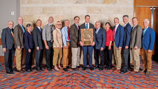
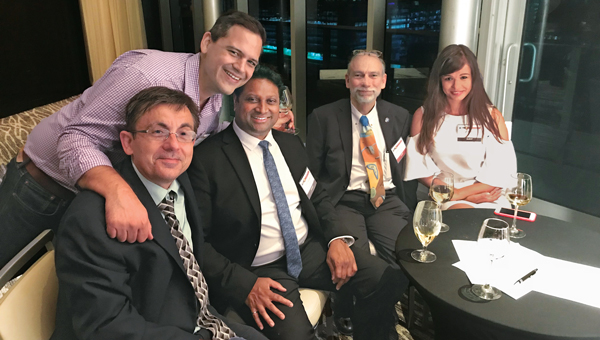
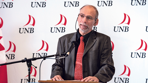
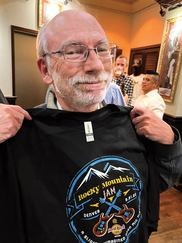
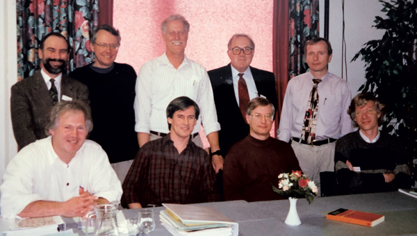
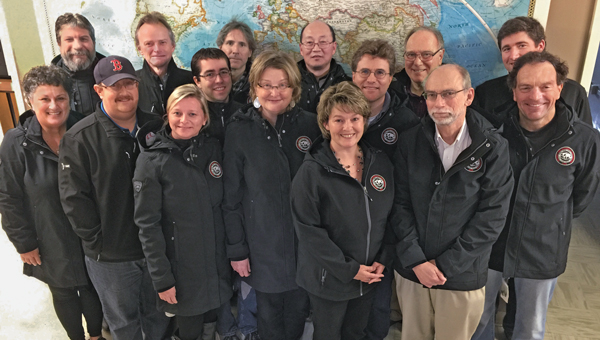
    The November 2024 issue of GPS World features Professor Richard Langley’s 300th and final “Innovation” column. His first one appeared in the January/February 1990 issue, the magazine’s very first. In celebration of Richard’s decades-long contribution to GPS / GNSS / PNT, we are publishing a selection of testimonials and photos (below) from some of his colleagues and friends, gathered by his former students Sunil Bisnath and Attila Komjathy.


    Recollection from 1990, Trinidad – University of the West Indies

    It was 1990, late into a — thankfully warm — night in Trinidad. I still remember that moment vividly — the sense of anticipation mixed with skepticism. A small group of us, undergraduates from the Land Surveying Department at the University of the West Indies, were standing outside in the middle of the night. We were waiting, eyes fixed on the sky, holding our breath for signals that were promised to come — signals that the foreign professor, Richard Langley, assured us would soon appear and change our lives forever. Back then, GPS satellites were in scarce supply. Only a few were up there, and getting a signal was not guaranteed. Richard’s confidence, however, was unwavering. He was convinced that this technology — this new way of understanding our position in the world — would revolutionize everything we knew about land surveying and navigation. That year was my last in Trinidad. I left with memories of those nights under the stars, waiting for those elusive signals that did eventually come. Over time, I’ve met Richard at numerous Institute of Navigation events, and like the GNSS constellations, we have continued to grow and evolve yet remain united by our passion for a technology that continues to grow beyond our wildest expectations. – Professor Allison Kealy, FRIN, GAICD Director, Innovative Planet Research Institute Professor, Civil Engineering Swinburne University of Technology


    I was introduced to Richard more than 15 years ago. I learned quickly that he is not only a man of renown earned by his overarching knowledge on almost all aspects of satellite navigation, but also a man of action. Not surprisingly and probably well known, he was one of the first researchers investigating and improving the Precise Point Positing (PPP) technique. It is less well known that he was also an early adopter of the PPPPP concept. When asked what the abbreviation stands for, Richard would answer with a twinkle in his eye: “Proper preparation prevents poor performance!” I had the honor of seeing Richard in action during a joint measurement campaign where we applied both concepts. We wanted to collect observations of the new Galileo test satellites GIOVE-A and -B to use them for precise positioning. It happened that they had favorable visibility during the ION GNSS conference in Savannah, Georgia, in September 2009. So, we mounted a bunch of equipment onto Richard’s rental car and off we went through the streets, after carefully making sure that the GIOVE satellite were actually visibile and reference product generation back home in Munich, Germany, and New Brunswick, Canada, was properly working. Richard was steering the automobile in rapid turns on the parking lot to get some serious phase wind-up effect going. I was so concentrated on the data logging that I did not even feel the urge to throw up. The measurement collection went well and the data ended up being used for a joint publication the following year, potentially one of the first papers jointly using GPS and GIOVE. PPP using the PPPPP rule — there you go! – André Hauschild, Ph.D., Researcher German Aerospace Center (DLR)


    I first knew of Richard Langley through his Innovation column in GPS World. It was largely through this column that I acquired my basic knowledge of GPS. The columns were always so clear and so well written. It was a time of rapid change — the Internet, rapid data transfer between sites, and many, many other challenges. I received a grant to fund the Westford Water Vapor Campaign, and along with Arthur Niell of Haystack Observatory, we set out borrowing as many receivers, radiometers, and radiosondes as we could. Thus began my first “international” phone call to Richard Langley (the University of New Brunswick is, of course, in a foreign country) asking him to borrow receivers. Richard, perhaps because he did his postdoc here at MIT, and spent many hours out at Haystack, was more than amenable. He not only lent us three receivers but also a foreign visitor, Pieter Toor from Delft, and Virgilio Mendes, one of his graduate students. From them I learned immeasurably about the troposphere and water vapor distribution. The Westford Water Vapor Experiment was an important series of measurements, that helped us realize the potential of GPS before it was fully recognized by the community. Later, I was invited to join Jack Klobuchar and the Canadian equivalent of the FAA to fly to the University of New Brunswick, where I met Attila Komjathy for the first time. Later I also came to know Sunil Bisnath. Richard Langley trained a remarkable set of students, many (if not most) of whom have gone on to stellar careers. – Anthea J. Coster, Ph.D., Assistant Director; Principal Research Scientist MIT Haystack Observatory


    Professor Richard Langley is truly one of the masters of the GNSS community. He has been the mainstay of knowledge, scholarly activity, and mentoring to scholars and students for decades. His friendly demeanor and wiliness to help out wherever he can, makes him a pleasure to talk to and collaborate with. I look forward to seeing Richard at ION technical conferences with that big smile on his face and observing his love for and devotion to the art and science of navigation. – Professor Chris G. Bartone, Ohio University


    Richard and I are of the same “vintage” (date/time: referring to the period when we ramped up our work and study activity) and “terroir” (space/environment: referring to discipline background, circumstances and opportunities). We were both educated as surveyors, we both became academics, and we both mastered the arcane applied science field of geodesy. Geodesy in the 1970-1980s was undergoing a revolution driven by advances of the Space Age, reflected in the increasing use of Earth-orbiting satellites for precise positioning, mapping, gravity field determination, sea surface mapping, and much more. Richard and I are of the generation of geodesists in the 1980s that recognized — before any other engineering or science discipline — that GPS was going to change our world in profound ways. We pioneered its use for geodetic surveying (at the sub-cm accuracy level) even before GPS was declared “fully operational” in the mid-1990s. We had more than a decade head-start in understanding the principles of differential GPS, of carrier phase-based static positioning, and of the system itself. It is a head-start that continues to this day. We developed the first university GPS courses, wrote the first textbooks, educated the first generation of GPS scientists, developed the first measurement processing software, and helped revolutionize the practice of navigation. Although GNSS is considered the most important geoscientific technology that we use today, precise GNSS-enabled positioning has impacted so many other professional, scientific and social applications. With the founding of GPS World’s “Innovation” column, Richard launched an amazing educational and industry outreach service. Those articles tracked the advances in GPS/GNSS technology and applications. While there are still some of our geodesy generation making contributions to their discipline, Richard has continued to promote GNSS for 35 years in a unique way, through his careful curation of “Innovation” column articles. They remain a joy to read. Richard, keep up this great service to the positioning, navigation and timing (PNT) community. – Professor Chris Rizos, President International Union of Geodesy & Geophysics (IUGG) School of Civil & Environmental Engineering UNSW Sydney Australia


    I have had the pleasure of knowing Richard since the mid 1980s, when we were part of the team that produced the first and highly successful book on GPS, namely the Guide to GPS Positioning. We have interacted regularly ever since. I have always appreciated reading Richard’s papers for their clarity, thoroughness and novel content. His Innovation column in GPS World for 35 years is now a GPS classic that post-graduate students and experts alike learn from and enjoy reading. Richard has deservedly received major awards for his numerous and outstanding work. Richard, I hope that we will continue to benefit from your contributions for years to come. – Professor Gérard Lachapelle, University of Calgary


    Despite being a highly respected leader in the field of PNT, Richard remains a humble human being. He sets a high standard for his work and is generous with his time to catch even the smallest errors in research papers. It has been a great pleasure to get to know him and to have the opportunity to work with and learn from him. He is an inspiration and a role model for me. – Professor Jade Morton, Ph.D., Helen and Hubert Croft Professor Ann and H.J. Smead Aerospace Engineering Sciences Department University of Colorado Boulder


    I have had the privilege of knowing Prof. Richard Langley for my entire career in PNT and have always been greatly impressed with his wealth of knowledge and research on high-precision applications of GPS. I first met him in the late 1980s at meetings of the Civil GPS Service Interface Committee (CGSIC) and the early Institute of Navigation conferences on GPS in Colorado Springs. When I joined the navigation team at the U.S. Department of Transportation as a young engineer in 1988, we all had copies of The Guide to GPS Positioning, that Prof. Langley co-authored with David Wells and that we greatly utilized! Since that time, I have enjoyed interfacing with Prof. Langley at ION conferences and serving with him on the ION Council. I have learned so much from his research, including his development of the UNB-RTK system and the study of atmospheric effects for the FAA Wide Area Augmentation System (WAAS), as well as the very informative articles he has published in GPS World! – Karen Van Dyke, Director, Positioning, Navigation, and Timing U.S. Department of Transportation


    The 35-year anniversary of Richard’s Innovation column in GPS World seems amazing, also recalling the recent 30-years celebration of the International GNSS Service (IGS), which to many of us seemed like an eternity. This is not surprising, however: from the Guide to GPS Positioning, co-authored by Richard (my first GPS handbook when I started learning about GPS in November 1989 at ICC, Barcelona); to the knowledge, motivation and empathy we have always enjoyed when meeting Richard in so many different workshops (ION, Beacon Satellite…) and collaborative works (e.g., IERS Conventions…). For him, this is normal. CONGRATULATIONS. – Professor Manuel Hernandez-Pajares, UPC-IonSAT, IEEC-CTE Head of the UPC-IonSAT Research Group, IGS Associate Analysis Center Department of Mathematics, Universitat Politècnica de Catalunya, Barcelona, Spain


    Professor Langley has been a vital contributor to the Institute of Navigation (ION) for four decades, serving in various volunteer and leadership capacities. In his most recent role, Richard has served as the Editor-in-Chief of NAVIGATION, The Journal of the Institute of Navigation, our esteemed peer-reviewed technical publication. Since taking on this role in 2020, he has expertly led a team of associate editors, guiding NAVIGATION through a transformative period as it transitioned from a traditional print publication to a fully open-access journal. Under his leadership, the journal has seen a remarkable increase in its impact factor, most recently rising to 3.1. Beyond his editorial work, his most important contribution lies in his mentorship. He has profoundly influenced the next generation of GNSS experts, nurturing countless graduate students through ION’s programs and initiatives while fostering their professional development. His dedication to education and commitment to innovation has enriched our community. We deeply value our ongoing collaboration with Richard. His unwavering commitment, expertise, and passion for GNSS and ION have made him an integral part of our organization. It is a privilege to work alongside such a dedicated professional. – Lisa Beaty, Executive Director Institute of Navigation


    Like many others, I look back to a long friendship with Richard, who’s always been a mentor and model for me. His sharp mind, paired with a distinct sense of very British humor makes each meeting with him a source of inspiration and memorable experience. From gentle spelling and grammar corrections in manuscripts to advice and leadership in GNSS-related projects, he always offers a helping hand, contributes in-depth knowledge and one or another personal anecdote. From him, I learned the “six P” rule: proper planning and preparation prevents poor performance. This unforgettable saying not only reflects the rigor Richard applies to his work, it also provided me a guideline that I’m now passing on to my own students. – Oliver Montenbruck, Ph.D. Head, GNSS Technology and Navigation Group German Aerospace Center (DLR)


    I would like to say, as someone who is not his direct advisee, I’ve always appreciated his avuncular spirit, mentorship, and encouraging guidance over the years. I join you in toasting to him and his successes in growing and connecting the navigation community over his many years of service, in addition to all his technical achievements and innovations. Cheers to Richard! – Professor Seebany Datta-Barua Illinois Institute of Technology


    Richard has been a highly respected leader in the GNSS community for more than 30 years, making his mark as a creative innovator, a mentor for generations of future leaders and contributors to the advancement of GNSS, and as an insightful and patient teacher. The well-worn copy of his Guide to GPS Positioning on my bookshelf has helped me and countless students quickly pick up the basics, while his cheerfully engaging series of “Innovation” columns in GPS World explored every feature, misconception, novel application, mystery, and intricacy of GNSS. And, he literally put Fredericton on the map for the GNSS community. – Penina Axelrad, Distinguished Professor University of Colorado


    When I became GPS World’s managing editor, in 2000, my exposure to GPS was limited to a few journal articles I had read as a graduate student in international security at MIT in the mid-1990s. Much of my education on the subject during the steep learning curve that followed came from Richard’s “Innovation” column. Also, as his liaison to the magazine, I was responsible for entering his many, meticulous edits to each column, which, at the time, he sent me by fax. Nearly a quarter century later, Innovation is still my favorite section in the magazine. I will miss it greatly.” – Matteo Luccio, Editor-in-Chief, GPS World


    Good memories of my collaborations with Richard span a long time to almost the operational beginnings of GPS. Examples range from our collaboration on the Handbook for GNSS to our shared lecturing at the “GPS for Geodesy” school, in Delft, 1996. I always experienced with admiration Richard’s encyclopedic knowledge and excellent lecturing and writing skills. The only one thing that I would have wished for is that Richard would have turned his excellent Innovation columns in GPS World into a book. That would have been a bestseller for sure. – Professor Peter Teunissen Delft University of Technology


    I first met Richard in 1982 while a postdoc at MIT about the time that he joined the faculty at the University of New Brunswick, after his postdoc in the same MIT department. After research in VLBI and SLR, he was one of the early pioneers in the development of GPS for precise positioning applications, with contributions in several areas, such as signal multipath and tropospheric refraction. We both taught at the International School of GPS for Geodesy in Delft, first in 1995, and contributed to the resulting monograph, GPS for Geodesy. I have a vivid memory of drinking beer with him in a bar in Delft after a long day at the school. – Professor Yehuda Bock Scripps Institute of Oceanography


    I first met Richard shortly after joining MIT as a Ph.D. student in 1979. He was a postdoctoral fellow for two years with MIT’s Department of Earth and Planetary Sciences, carrying out research in geodetic applications of lunar laser ranging and very long baseline interferometry after completing his Ph.D. at York University, Toronto. His research at MIT led to the discovery of a 50-day oscillation in atmospheric angular momentum and length of day determined from lunar laser ranging data. This work was published in 1981 in Nature. Richard has been publishing impactful papers on important topics since very early in his career. His contributions to GPS World’s “Innovation” column have followed that trend. – Professor Thomas Herring Massachusetts Institute of Technology


    I did not have tons of personal contact with Richard, but the contact I did have showed me that he was a man of very high standards, and it’s clear that his dedication to the field is enormous. The combination of high standards and selfless dedication is what moves us forward. He also attracted and produced a cadre of highly talented and successful researchers that continue to have an enormous impact on the field. These are great things! – Anthony J. Mannucci, Ph.D. Deputy Manager, Tracking System and Applications Section Jet Propulsion Laboratory


    Years ago when assembling material for my advanced GNSS signal processing course here at the University of Texas, I found that for several topics Richard’s “Innovation” column had just the discussion and analysis I was looking for my students to learn. His writing is unfailingly engaging and lucid! What a gift to the community his “Innovation” column has been! Richard is an amateur radio enthusiast. Many of the insights on radio in his columns are backed up by his practical experience with long-distance ham radio communications. He’s connected with people from continents away from his home base in New Brunswick. – Professor Todd E. Humphreys, Ashley H. Priddy Centennial Professorship in Engineering Dept. of Aerospace Engineering and Engineering Mechanics The University of Texas at Austin


    I first met Richard Langley in 1989 at what was my first ION Satellite Division meeting. It was a young-looking crowd, but we both could pass for young men then. I also met another young man by the name of Glen Gibbons who was circulating among the attendees to gauge interest in a trade magazine devoted to GPS that he was thinking of launching. GPS World played an important role in my career as a GPS engineer, particularly for its “Innovation” column, edited by Richard. His early columns (such as “Why is the GPS Signal So Complex?”) are classics of cogent writing and served as an inspiration to me when I tried my hand at writing about GPS. His skills as an editor, and his generosity to help a friend avoid embarrassing himself, proved even more helpful to me. My debt to Richard has grown over the years, and so has my admiration and affection for him. – Professor Pratap Misra, Professor of the Practice of Mechanical Engineering Tufts University


    When I googled “Richard Langley,” just for fun, I got multiple returns — among them “professional football player,” “state politician,” “actor,” “model maker” and I thought for a while that those are Richard’s other personalities that I didn’t know about. Well, a slight refinement of my search “Richard Langley, geodesy” got me what I was looking for — pages and pages on the accomplishments of the Richard Langley as one of the first scientists who recognized the great potential of GPS as a scientific and civilian tool and an everyday commodity, research publications that all GPS “insider wannabees” have read and memorized, and articles documenting his commitment to GPS World, especially its “Innovation” column — which has long been one of my favorite reads. I congratulate Richard on the 35th anniversary of this outstanding column! – Professor Dorota Grejner-Brzezinska, Vice-Chancellor for Research at University of Wisconsin-Madison


    Richard and I first met when I spent a post-doc year at the University of New Brunswick in 1983/84. The nucleus of the Bernese GPS software emerged from this visit. Richard and I became friends and stayed in contact after this visit. We met last time in Bern at the 2024 IGS Symposium commemorating 30 years of the International GNSS Service. What I admire most about Richard is his scientific breath and his at times artistic use of the English language — he announced his visit to Bern with the words “I will be there if I don’t ‘keel over’ between now and then.” – Professor Gerhard Beutler University of Bern


  • Innovation Insights: What is carrier phase?

    Innovation Insights: What is carrier phase?

    Innovation Insights with Richard Langley
    Innovation Insights with Richard Langley

    WHAT IS CARRIER PHASE? The obvious answer is: the phase of the carrier. But this is not helpful if you don’t know what a carrier is. A carrier is basically a harmonic electromagnetic wave — a pure continuous sinusoidal wave with a single constant frequency and amplitude.

    Such a wave has limited uses. However, if we modulate or change the characteristics of the wave in some way, then the wave can carry information. Changing the amplitude by using a voice or music audio signal is amplitude modulation as used for AM radio.

    Instead, one could modulate a carrier by changing its instantaneous frequency, which is frequency modulation or FM and is used for high-fidelity broadcasting. Yet another way to modulate a carrier is to change the instantaneous phase of the carrier, and that is how GNSS works.

    GNSS carriers are phase-modulated by pseudorandom noise (PRN) codes and navigation messages. A GNSS receiver uses the PRN codes to produce the pseudorange observable with a precision in the tens of decimeter range. This is the most common observable for GNSS positioning.

    But by stripping away the modulation of the received GNSS signals, the receiver can measure the phase of the underlying carrier. Changes in carrier phase over time reflect the change in the (pseudo)range but are about two orders of magnitude more precise.

    One problem with carrier-phase measurements is that they have an initial cycle ambiguity that must be resolved, preferentially fixed to the correct integer value, before they can be used for positioning, but this can be achieved without too much difficulty. While fixing the ambiguity of carrier-phase measurements might be considered a nuisance in GNSS positioning, it can help detect spoofing of GNSS signals where some other techniques might fall short.

    In this “Innovation” column, we look at how carrier-phase measurements combined with those from an inertial measurement unit can guard against a deliberate attack on an automated ground vehicle — something that cannot be discounted in our world these days.

    Read the full “Innovation” column: GNSS Spoofing Detection: Guard against automated ground vehicle attacks.

  • Innovation: Software-defined radios for GNSS

    Innovation: Software-defined radios for GNSS

    A Step-by-Step Exposition of an Educational Resource

    Innovation Insights with Richard Langley
    Innovation Insights with Richard Langley

    THE RADIO. It’s been around for more than 100 years. Pioneering work by Guglielmo Marconi and others in the1890s and 1900s resulted in practical wireless telegraphy devices that permitted point-to-point communications with ships at sea and between stations on land hundreds and thousands of kilometers apart and even between stations on different continents. The first radio broadcasts (point-to-multipoint) were time signal transmissions and weather broadcasts. Experimental audio transmissions took place in the early 1900s, and by 1920 or so, radio stations were established in many countries for broadcasting speech and music to the general public.

    The first radio receivers were simple crystal sets. It wasn’t until the mid-1920s that tube radios became commercially available. Eventually, tubes were replaced by transistors, and transistors by integrated circuits. The introduction of microprocessors resulted in digital receivers, with the conversion of the received analog radio signals into audio being carried out digitally for the most part.
    One of the latest advances in radio technology is the software-defined radio or SDR. An SDR typically consists of two components: a piece of hardware, called a radio frequency (RF) front end, and a piece of software run on a general-purpose computer. The job of the front end is to convert a portion of the radio spectrum received by its antenna to a digital data stream processed by the software. The software decodes the data to produce the desired result. Since the software does most of the “heavy lifting” in processing a radio signal, it is often called the SDR itself. And by the way, there are SDR transmitters, too.

    It should come as no surprise that SDR technology has come to the GNSS field. In fact, in 2007, the seminal text on GNSS SDRs, A Software-Defined GPS and Galileo Receiver: A Single-Frequency Approach, was published along with the sale of an inexpensive RF front-end in a thumb-drive-sized package that allowed graduate students and others to experiment with a GNSS SDR themselves. And we have covered GNSS SDR developments in this column from time to time, most recently in January 2018 (“The Continued Evolution of the GNSS Software-Defined Radio: Getting Better All the Time”).

    In this month’s column, researchers from the lab that helped produce the SDRs documented in the 2007 book (which is still in print) discuss their development and testing of additional freely available SDR codebases covering all four GNSS (GPS, Galileo, BeiDou and GLONASS). They provide an excellent resource for learning how GNSS receivers actually work.


    By Joan Bernabeu, Nicolas Gault, Yafeng Li and Dennis M. Akos

    With the publication of the book A Software-Defined GPS and Galileo Receiver: A Single-Frequency Approach by Kai Borre, Dennis Akos and their fellow authors, an open-source GNSS software-defined radio (SDR) receiver developed using Mathwork’s Matlab language was made available, together with sample data sets that facilitated the testing process for all interested readers. The first SDR implementation focused on processing the GPS L1 C/A-code legacy signal and served as a starting point for students and researchers in the Radio Frequency (RF) and Satellite Navigation Laboratory at the University of Colorado Boulder, where later activities aimed to improve the software code and add new features as new GNSS signals emerged. As a result, the initial codebase evolved into a complete collection of SDRs capable of processing all GNSS signals from every satellite constellation, with BeiDou’s B1I, B1C, B3I and B2a signals the latest additions. The most recent efforts were dedicated to collecting all SDR codebases, putting them in a common format, and testing them to give an account of their performance. This article describes our efforts, placing special emphasis on explaining the test framework designed to test each SDR, as well as on reporting the adjustments made and the results obtained. GPS test cases have been taken as examples to show how some SDRs were assessed when issues were found in the results they provided.

    OPEN-SOURCE GNSS SDR COLLECTION

    The whole SDR collection has been developed in Mathwork’s Matlab programming language. To run the code and perform tests, users simply require an active Matlab license and the software available on their computer. Once these requirements are met, the user can choose to download any of the available codebases and the corresponding data set to start experimenting. 

    We recommend using version control software to keep track of changes made to the original version of the code. Users should consult the Borre et al. text for further details on running the codebases.

    A total of 12 SDR codebases are aimed at processing each of the GNSS signals (see TABLE 1). All code files for each SDR are organized in the same subdirectories, and most of them have the same filenames. 

    Table 1. All GNSS signals that can be processed by the SDR collection, organized by their corresponding satellite systems.
    Table 1. All GNSS signals that can be processed by the SDR collection, organized by their corresponding satellite systems.

    All SDRs are set to work with a default configuration. They are all run using an init.m script, which collects user settings (input data file path, sampling frequency and so on) from the initSettings.m configuration script. Given this, the first file that users may want to modify is initSettings.m, to define the run settings for a given test. Most of the SDRs operate in an identical way, however some include particular features oriented at exploiting certain characteristics of the corresponding GNSS signal. The GPS L2C SDR, for example, gives the user the option of whether to process the pilot component of the signal.

    The test samples available in the public directory were obtained in accordance with the characteristics depicted in TABLE 2 for every signal. The first two columns from the left show all the signals the SDR collection can process and the central carrier frequency at which they are transmitted. The third column gives the bandwidth selected in the recording process for every signal. This value must match the sampling frequency defined in the initSettings.m file for each SDR. Only three frequency bandwidths can be used to record GNSS data, so as to make the configuration structure more homogeneous across different SDRs. They were selected to ensure similar characteristics for each signal in terms of performance, encompassing most of the signal power for each modulation, but also keeping the recorded GNSS data files within a reasonable size.

    Table 2. Summary of the tested GNSS signals’ center frequencies and the selected bandwidth (BW) for their processing. The common IF for all signals is 20 MHz.
    Table 2. Summary of the tested GNSS signals’ center frequencies and the selected bandwidth (BW) for their processing. The common IF for all signals is 20 MHz.

    All the signals were mixed to a common intermediate frequency (IF) of 20 MHz in the recording process. Both the frequency bandwidth and the IF are fundamental to obtain the expected results from each SDR codebase. These are set in the settings file. The default configuration was validated in the testing campaign explained in later sections, and should only be modified to meet the user’s specific needs, being aware that some SDR performance characteristics may also be affected.

    BASIC GNSS SDR STRUCTURE

    While the general SDR receiver structure is similar across all codebases, each comes with adjustments and/or additions to adapt the code to the format of a specific signal. The general codebase structure can be summarized in four major modules:

    • signal acquisition
    • tracking stage
    • navigation data decoding
    • position, velocity and time (PVT) computation.

    An important remark is that the SDR collection developed is designed to process files of limited duration. The code is designed to use enough data to provide a successful initial acquisition, and then use a single set of satellites for the remaining execution. In other words, there is no extra logic oriented at acquiring or reacquiring satellites after the first acquisition is achieved.

    Signal Acquisition. The design of the acquisition scheme depends on the characteristics of the signal the SDR is aiming to process. There are numerous GNSS signal configurations for each constellation that follow different strategies concerning spreading codes, navigation data and secondary codes, which must be accounted for in the acquisition codebase.

    All codebases follow a fast Fourier transform (FFT) accelerated serial search-acquisition approach to obtain estimates of the signal’s carrier frequency and code delay, where a number of signal replicas are generated iteratively, separated by a defined frequency interval in the frequency domain. All the frequency offsets are arranged in what are known as frequency bins. This frequency separation will be referred to as the frequency step. The latter is inversely proportional to the integration time and tells the maximum error allowed in the carrier frequency estimate, which is half the frequency step. Both the frequency step and the coherent integration time are parameters that have a strong effect in acquisition results, as will be seen below.

    Each local replica is correlated with the input signal to obtain a code-phase estimate. The length of this correlation is the so-called coherent integration time. The maximum correlation measurement from all frequency bins is then divided by the second maximum found. This ratio is called the peak metric and is used in all SDRs to give a measure of the magnitude difference between the maximum obtained and the remaining correlation results. If the peak metric is not high enough, this implies that the maximum is close to other cross-correlation products and so could not correspond to the result obtained after correlating both input and local replica signals with the right code-phase alignment. When the peak metric surpasses the threshold defined in initSettings.m, the satellite is considered to be acquired. 

    It is worth noting that in all SDR implementations the local replica is constructed by concatenating a whole primary code and a block of zeros of the same length. This prevents navigation bit transitions from affecting the correlation results. For example, GPS L2C-CM SDR’s acquisition correlates 40 milliseconds of data with 20 milliseconds of pseudorandom noise (PRN) spreading code followed by 20 milliseconds of zeros (the zero padding technique). 

    Tracking Stage. The tracking stage is oriented at refining and keeping track of the code and carrier estimates provided by the acquisition stage as well as demodulating the navigation data. This is achieved using feedback loops organized in channels, which are typically referred to as tracking channels. There will be as many tracking channels as the number of satellites acquired. Each tracking channel makes adjustments to the corresponding local signal replica for the given satellite, so that it resembles the real received signal as much as possible. When the replica is sufficiently accurate, the tracking loop locks onto the signal, removes the carrier and spreading code components, and starts registering data bit transitions. The task of every tracking channel is to account for signal variations so that they can keep locked on the signal for as long as the satellite is available for use.

    Tracking channels implement two feedback loops, the delay lock loop (DLL) and the Costas phase lock loop (PLL). The former is focused on the signals’ code phase while the latter on the carrier phase. These modules depend on two major parameters that determine the properties of the loop filter: the damping ratio and the noise bandwidth. On the one side, the damping ratio controls how fast the filter reaches the settling stage. On the other side, the noise bandwidth informs the amount of noise allowed in the filter.

    While all SDRs follow similar tracking loop schemes, some signals, such as GPS L2C, need some adjustments to the parameters mentioned above so that they provide the expected results, as we point out later. Tracking results are stored in a Matlab .mat file, but also can be assessed in the plot the tracking stage generates after it finishes processing all the channels.

    FIGURES 1a and 1b show an example of two different tracking results plots, each of which include seven figures. These show the in-phase/quadrature (I/Q prompts), the navigation data bits decoded, the changes in the raw/filtered Costas loop and DLL discriminators, and the early-prompt-late metrics. Note that the plots in Figure 1a suggest the navigation data bits were demodulated successfully. In contrast, in Figure 1b, data bits cannot be distinguished because the tracking stage failed to demodulate the navigation message.

    Figure 1. (a) shows the plot generated for a successful tracking channel. In contrast, (b) illustrates the results obtained when the tracking loop in question did not lock appropriately to the signal and therefore was not able to demodulate navigation data. (Image: Authors)
    Figure 1. (a) shows the plot generated for a successful tracking channel. In contrast, (b) illustrates the results obtained when the tracking loop in question did not lock appropriately to the signal and therefore was not able to demodulate navigation data. (Image: Authors)

    Navigation Data Decoding. This stage extracts the navigation data required by the SDR codebase to compute PVT estimates from the results delivered by the tracking stage. The latter outputs I/Q prompt samples representing data bits, containing the encoded navigation data. The navigation data format for each signal can be found in the interface control document issued by each satellite constellation operator.

    The general process that each SDR implements to demodulate navigation data from I/Q samples is summarized as follows:

    1. detect a preamble within data bits
    2. arrange the bit sequence in the corresponding structures, such as frames
    3. remove secondary code if present
    4. de-interleave and decode
    5. check if the bit stream has errors
    6. extract navigation parameters

    Once navigation parameters are extracted, they are stored and later used by the functions involved in the PVT computation stage.

    PVT Computation. The PVT stage takes the decoded navigation data, computes satellite positions, and solves the geometry problem, whose solution is the receiver’s location.

    As with all the other stages, all SDRs follow the same approach, and use the least-squares method to solve for a position estimate once all the data is available. Position estimates are delivered in both Earth-centered Earth-fixed and east-north-up coordinates.

    Similarly to the tracking stage, the PVT computation stage returns a plot showing some PVT statistics to help the user get an idea of the PVT performance of the test conducted. FIGURES 2a and 2b show an example of two positioning plots obtained for two different data files. 

    Figure 2. (a) shows the plot of a priori, good statistics for the navigation solution; (b) shows a navigation plot for a file that presented a problem affecting the PVT solution. (Image: Authors)
    Figure 2. (a) shows the plot of a priori, good statistics for the navigation solution; (b) shows a navigation plot for a file that presented a problem affecting the PVT solution. (Image: Authors)

    EXPERIMENTAL SET-UP AND TESTING

    In this section, we present the equipment we used in our tests (see FIGURE 3) and detail the process we followed to collect GNSS data, as well as the testing framework designed to exercise the SDR collection. 

    Figure 3: The antenna was connected to the RF port of the USRP. The USRP sampled the analog data delivered by the antenna using the TCXO as the reference oscillator. The resulting sampled data was stored in a Linux-based computer. (Image: Authors)
    Figure 3: The antenna was connected to the RF port of the USRP. The USRP sampled the analog data delivered by the antenna using the TCXO as the reference oscillator. The resulting sampled data was stored in a Linux-based computer.
    (Image: Authors)

    RF Antenna. The device used to sense the RF GNSS signals was a Trimble Zephyr2 antenna, which has enhanced capabilities for multipath minimization as well as low-elevation-angle satellite tracking properties. 

    The antenna was installed on the rooftop of the Ann and H.J. Smead Department of Aerospace Engineering Sciences building at the University of Colorado Boulder.

    USRP and TCXO Devices. An Ettus Universal Software Radio Peripheral (USRP) B200 hardware SDR connected to an IQD temperature-compensated crystal oscillator (TCXO) was used to collect digital samples from GNSS analogue signals sensed by the antenna.

    The B200 device was controlled by means of the USRP hardware driver (UHD) through a computer running a Linux operating system. UHD is a software application programming interface (API) that enables the development of code to manage USRP settings and operation. 

    PC Setup. The PC setup consisted of a Linux computer  with all the required drivers and program dependencies, as well as with Mathworks’ Matlab software installed. Matlab was used to program and automate the data recording process.

    Recording Process. The equipment described in previous subsections was used to record data suitable for each SDR codebase. The process to obtain signal data for all 12 codebases was reduced to eight stages by selecting an adequate frequency bandwidth, as some signals share the same central carrier frequency (see Table 2).

    For each stage, a total of 100 files with 61 seconds of I/Q GNSS data were recorded over a 24-hour time period. The I/Q samples recorded by the USRP were formatted as 8 bit sine carriers. All the data sets recorded are available together with a description file based on the Institute of Navigation’s metadata standard for GNSS.

    TESTING FRAMEWORK

    The workflow we followed to test every codebase from the collection is outlined in the following steps:

    1. Record data samples. A set of one hundred files were recorded with 61 seconds of GNSS data.
    2. Debug the SDR with the selected files. A debugging stage preceded every test case to ensure the codebase performed well enough, or else to make the required adjustments.
    3. Run the SDR for one hundred trials. A total of one hundred tests, one per file, were performed for all SDRs.
    4. Log metrics and present results. The results from all SDR stages (acquisition, tracking and data demodulation) were stored for each file. Also, each iteration returned a message that summarized the execution results.

    All of the messages returned for every file corresponded to one of the cases summarized as follows:

    1. Codebase issue. Message type returned when the codebase failed because of a coding issue.
    2. No navigation solution. The codebase was not able to deliver a navigation solution either due to a malfunction of the codebase or due to a lack of satellite availability. Navigation solutions are only available when both the tracking channel and the navigation data demodulation stages are successful for more than three satellites.
    3. Navigation solution with accuracy worse than 30 meters. A position solution fix more than 30 meters (in three dimensions) from the known antenna location was considered a non-accurate estimate.
    4. Navigation solution with accuracy under 30 meters. When the 3D positioning error was < 30 meters, the navigation solution for the position was considered accurate.

    All codebases passed a debugging stage before being tried with the whole set of available data. This was done to ensure that they performed as expected, and were able to achieve the required performance in terms of the metrics mentioned above in this section. An example of this debugging stage will be explained in further detail below. We take the GPS L2C codebase as an example of how all implementations were assessed in an attempt to improve their initial performance and make them more robust to code errors. See our proceedings paper for further details of our test cases.

    GPS L2C Test Case. The problem observed for GPS L2C was that some satellites acquired with a high acquisition metric were failing the tracking stage. The result was that no navigation data was demodulated from them. An in-depth study was required to find out the adjustments needed in the codebase that would help to solve this issue.

    The GPS L2C signal encompasses two signal components called civil moderate (CM) and civil long (CL). The CM component is formed by a spreading code that modulates a navigation message. The CL component is a pilot (data-less) signal modulated with a longer spreading code allowing for longer coherent and non-coherent integration times, yielding better sensitivity. 

    For CM signal acquisition, the 20 millisecond code length limits the coherent integration time to 20 milliseconds, due to the overlaid navigation message. This integration time defines the minimum frequency resolution required to obtain the expected correlation results. The CL component is used in the SDR to accumulate consecutive correlation results non-coherently, contributing to the receiver’s sensitivity by allowing it to operate with higher acquisition metrics in general.

    The initial configuration for this SDR codebase is represented in TABLE 3a.

    Table 3. Configurations for GPS L2C test case.
    Table 3. Configurations for GPS L2C test case.

    With this configuration, a total of 10 satellites were acquired. However, it was observed that for some satellites acquired with high peak metrics, it was not possible to demodulate their navigation data, and thus they were not considered for the navigation solution in later stages. This situation was abnormal, as typically this behavior is more characteristic of weaker signals whose bit transitions are too noisy to be decoded. This problem suggested that either the code-phase or the carrier frequency estimates (or both) were not accurate enough for each tracking channel to generate a proper replica to lock onto the input signal.

    The first step taken to address this matter was to inspect the SDR’s acquisition stage for a file presenting the mentioned problems. For instance, taking a closer look at the carrier and code-phase 3D representation for those satellites acquired with a high acquisition metric that were not successfully tracked afterwards. After doing so, some satellites were identified with the irregular characteristics described above, as for example the PRN 10 satellite. PRN 10 is taken as a reference throughout this subsection.

    The metric analyzed for PRN 10 was the matrix built by the acquisition’s serial search process. This matrix contains the correlation results obtained for each frequency bin. The width of each frequency bin is determined by the frequency step size defined in the configuration file. In this way, the smaller the frequency step, the more frequency bins that the corresponding matrix contains. This implies a better frequency resolution. 

    With this in mind, the frequency resolution was progressively increased by decreasing the frequency step size. Extra logic had to be added to the acquisition algorithm to implement this feature. It was found that when using a step size of 6.5 Hz, the tracking stage was then able to lock and demodulate navigation bits from PRN 10 effectively. This was the most significant determining factor to overcome the issue in question for the majority of the satellites available. However, other smaller adjustments also improved tracking results in general. These are depicted in TABLE 3b.

    CODE AVAILABILITY

    All the resources concerning the SDR collection are publicly available at the portal hosted by University of Colorado Boulder. Through this portal, all the GNSS codebases along with the data sets for testing can be acquired, as well as access to the discussion forum.

    CONCLUSION

    The first version of the SDR collection was made available after the seminal text by Borre et al. was published and consisted of a GPS L1C/A SDR and multiple data sets. From then on, this project kept evolving by adding more SDRs as new GNSS signals emerged across different satellite constellations.

    Our most recent work was to collect all the SDR codebases, arrange them in a common format, and test each implementation to assert their robustness and extract statistics concerning their performance.

    Future work will be dedicated to adding more features aiming at refining the PVT estimates delivered by each SDR.

    More progress is expected to be made soon, with additional improvements made in the GNSS laboratory. In addition, there is plenty of room for contributions from other researchers who want to support and collaborate with this open-source initiative. Our portal provides a convenient way to manage these contributions.

    ACKNOWLEDGMENTS

    We thank the many individuals who collaborated in the development of the open-source GNSS SDR collection. 

    This article is based on the paper “A Collection of SDRs for Global Navigation Satellite Systems (GNSS)” presented at ION ITM 2022, the 2022 International Technical Meeting of the Institute of Navigation, Jan. 25–27, 2022. 


    JOAN BERNABEU is a Ph.D. student at the Institut Supérieur de l’Aéronautique et de l’Espace, Toulouse, France. He also works as a satellite navigation engineer for GMV, Spain.

    NICOLAS GAULT is a Ph.D student at École Nationale d’Aviation Civile, Toulouse, France. He was a visiting scholar in the Department of Aerospace Engineering Sciences at the University of Colorado (CU) Boulder in 2020-2021.

    YAFENG LI is an associate professor in the School of Automation at the Beijing Information Science and Technology University, China. He was a visiting researcher with the Department of Aerospace Engineering Sciences, CU Boulder in 2017–18.

    DENNIS M. AKOS is a faculty member in the Department of Aerospace Engineering Sciences at CU Boulder.

  • GPS plays role in black hole image

    Headshot: Tracy Cozzens
    Tracy Cozzens

    On April 10, the world looked in awe at the first image of a black hole. The image was captured by a world-spanning network of radio telescopes that together, using Orolia atomic-clock technology, create the Event Horizon Telescope.

    It zeroed in on the supermassive monster — 6.5 billion times the mass of the sun — in Galaxy M87 to create the image.

    As Innovation Editor Richard Langley explains, the technique used to capture the image — very long baseline interferometry (VLBI) — relies on GPS. (VLBI was the topic of Langley’s Ph.D. thesis.)

    VLBI links two or more radio telescopes that can be many kilometers apart, or even on different continents. VLBI is used in both geodesy and astronomy. There is also a practical GPS link to the Event Horizon Telescope. From the second of six simultaneously published open-access papers on the result: “All timing is locked to a 10-MHz [hydrogen] maser reference and synchronized with a pulse-per-second (PPS) Global Positioning System (GPS) signal…”

    “[T]he long-term drift of the maser [is] compared to GPS, measured by differencing [and plotting] the 1 PPS ticks from the maser and local GPS receiver. The vertical width of the trace is due to variable ionospheric and tropospheric delays of the GPS signal, while the long-term trend represents the frequency error of the maser. The drift measured from this plot, and its effects on the fringe visibility, are removed during VLBI correlation.”

    Image: Event Horizon Telescope Collaboration
    Image: Event Horizon Telescope Collaboration

    From the third paper: “In order to reconstruct the brightness distribution of an observed source, VLBI requires cross-correlation between the individual signals recorded independently at each station, brought to a common time reference using local atomic clocks paired with the Global Positioning System (GPS) for coarse synchronization.”

    Read more about the image and GPS.

  • Happy Pi Day

    Happy Pi Day

    In honor of 3.14.2019, here is what GPS World’s Innovation column editor Richard Langley wrote about π in an article (“A Sideways Look at How the Global Positioning System Works“) nine years ago.


    3.1415926…. π. Every nerd’s favorite number. It is the ratio of a circle’s circumference to its diameter in conventional or Euclidean space. We use it, for example, to convert angles measured in radians to degrees (π radians = 180 degrees). π is an irrational number, which means that its value cannot be expressed exactly as a fraction m/n, where m and n are integers. Consequently, its decimal representation never ends or repeats. But we sometimes use an easily remembered fraction, such as 22/7, to get an approximate value. In this case, 3.14. But, if we compute more digits with this fraction, we get 3.1428571…, clearly an incorrect result. A better way to remember π to eight digits is to count the number of letters in each word of the mnemonic “May I have a large container of coffee?”

    In computations related to GPS, how many digits of π should be used? It depends. If you are developing your own algorithms and software for modeling GPS observations or determining precise orbits for the satellites, you’ll likely need π to 16 digits for double-precision floating-point calculations. But it would be a mistake to use π to this precision in computing the position of a satellite from the broadcast ephemeris. The GPS interface specification document, IS-GPS-200, specifies a 14-digit value for π (3.1415926535898) in the satellite coordinate computation. Use fewer or more digits, and the resulting satellite coordinates will not be as accurate.


    Full article here.

    Thank you, Dr. Langley.

  • Mining the magic “More” menu — again

    In April 2016, I introduced readers to useful features of our newly redesigned website at GPS World. This month, I want to again remind readers of all that we offer — features that may not be apparent if you just visit the homepage to read the news.

    In our redesign, we endeavored to make the website even easier to use. Part of that effort consolidated some of our most popular features under the More dropdown menu. The little word appears at the far right of the menu row under our logo. Within it is a world of data and information to explore.

    For those seeking current and historical data on the satellites in the various GNSS constellations, we have a full Almanac, which we update at least twice a year for the print magazine.

    If you want to stay on top of Upcoming GNSS Satellites Launches, we provide a handy table that is updated frequently by the one and only Richard Langley, our GNSS guru. Richard updates the table frequently — whenever new launch dates are announced.

    Richard also oversees the numerous and informative Innovation columns, all of which are available under the Innovation tab — right there under More.

    Our most current issue can be accessed through the words Digital Edition at the bottom of the page. Or, again under More, go to Magazine Archive for a full collection of every digital issue that reaches back a decade to 2005.

    Other great resources under More are our annual Receiver Survey and Antenna Survey. Both of these products are time intensive to produce, pulling together data and specs from almost 100 companies in an effort to provide a full picture of the products available and their capabilities.

    Similarly, the Buyers Guide link will take you to a special section on our website, allowing you to search manufacturers by product category and subcategory. Major updates of the Buyers Guide appear in print in June, but the online Buyers Guide is updated by companies year-round.

    If your company isn’t in our Buyers Guide, click on the “Add My Listing” link in the top right corner of the Buyers Guide page. It’s free!

  • Innovation: Orbit determination of LEO satellites with real-time corrections

    Innovation: Orbit determination of LEO satellites with real-time corrections

    Precision on Board

    INNOVATION INSIGHTS with Richard Langley
    INNOVATION INSIGHTS with Richard Langley

    SATELLITES. I have been fascinated by them ever since I was a child. My interest in satellites and space in general led me on my career path, which began with an undergraduate degree in physics at the University of Waterloo. Although it was an applied physics program and I did work terms at Atomic Energy of Canada, I was more interested in astronomy than nuclear physics and took all the astronomy courses I could. That, in turn, led me to pursue a Ph.D. in experimental space science doing research in the application of very long baseline (radio) interferometry (VLBI) to geodesy. As a postdoctoral fellow at MIT, I worked on ranging data from the U.S. and Soviet laser reflectors placed on the surface of Earth’s natural satellite — the moon.

    I continued my interest in VLBI and lunar laser ranging for a while after I arrived at the University of New Brunswick in 1981 but I quickly got involved with satellite Doppler positioning and that was when I heard my first satellite signals through the speaker of a Canadian Marconi CMA-722B Doppler receiver. At that time, Doppler positioning was being quickly supplanted by GPS and so my interest naturally migrated to the new system. GPS and the other global navigation satellite systems have been a consuming interest ever since.

    That interest includes helping to develop techniques for precision positioning and navigation — ones that minimize as much as possible the effect of various sources of error that plague GPS measurements. One such technique is precise point positioning or PPP, which uses primarily precise carrier-phase measurements along with an accurate model of those measurements to obtain position accuracies down to the centimeter level.

    Although often carried out with recorded data, PPP with real-time GPS orbit and clock correction streams has become an established technique for land, air and sea applications. However, the use of real-time corrections for precise positioning of satellites has not been attempted yet although a number of low-Earth-orbit (LEO) satellite missions could benefit from such a capability. Future satellites with altimeter and radio-occultation payloads may require real-time precise-orbit determination to enable onboard processing of science data for forecasting or now-casting of meteorology data, open-loop instrument operation of radar payloads, or quick-look onboard science data generation. Precise real-time orbit information could also be used for maintaining the formations of closely-spaced satellite constellations.

    In this month’s column, our authors discuss the results of realistic simulations they have carried out to precisely position a LEO satellite using a source of real-time GPS corrections actually transmitted by a network of geostationary satellites. Even accounting for data outages, 3D positioning accuracies better than a decimeter have been obtained. Precision on board? Not right now but likely coming real soon.


    Precise point positioning (PPP) with real-time orbit and clock correction streams has become an established technique over the past decade. Several free as well as commercial sources of precise correction streams are available through the internet or via a satellite link to geostationary satellites.

    Many applications exist for land, air and sea applications, but use of real-time corrections for precise positioning has not extended into orbit yet, although a number of low Earth orbit (LEO) satellite missions have a demand for precise orbit determination (POD). Mission requirements often allow for a relatively high latency for the availability of the precise orbit products, thus ground-based, near-real-time processing is sufficient. However, future satellites with altimeter and radio-occultation payloads may require real-time POD to enable onboard processing of science data for short-term forecasting or now-casting of meteorology data, open-loop instrument operations of radar payloads, or quick-look onboard science data generation. Also, precise real-time orbit information may be used for constellation maintenance of satellite formations. Despite early technology readiness demonstrations by the Jet Propulsion Laboratory carried out one decade ago to transmit real-time corrections via geostationary relay satellites to LEO spacecraft, this technique has so far not been implemented and used in a space mission.

    POD accuracy of a few decimeters or less with real-time corrections has been demonstrated repeatedly by various groups. For these studies, it was assumed that the required real-time precise orbit and clock products are continuously available on board the LEO satellite. Even though a network of several distributed geostationary Earth orbit (GEO) relay satellites may achieve seamless coverage in the equatorial region, gaps at high latitude close to the North and South Poles may occur. The extent of these gaps depends on the gain pattern of the transmitting antenna of the GEO relay satellite. Likewise, the availability of corrections depends on the LEO orbit characteristics, the gain pattern and mounting of the receiving antenna and the attitude profile of the LEO satellite. Most Earth observation and altimeter missions are launched into polar orbits to achieve global coverage. Up-to-date real-time corrections may therefore not be available for POD processing over the polar regions, which are typically also affected by reduced GNSS satellite visibility. As a result, the positioning performance will be degraded during this part of the orbit.

    To study the effects of interrupted availability of precise correction data, we simulated real-time POD using real flight data of the Swarm-C satellite, a representative LEO satellite orbiting Earth at an altitude of about 440 kilometers in a polar orbit with approximately 87° inclination. The satellite was launched into orbit in Nov. 2013 and is part of a three-satellite constellation of identical spacecraft with the mission objective to study Earth’s magnetic field and the electric field in the atmosphere (see FIGURE 1). The orbital period is 93 minutes. The satellite is equipped with a dual-frequency GPS receiver and two zenith-pointing POD antennas. The receiver provides dual-frequency GPS observations of up to eight satellites simultaneously. For the analysis, we selected a test data period of Feb. 1–15, 2016.

    FIGURE 1. Close-up view of the Swarm-C satellite with Swarm-A and -B in the background (artist’s impression). The satellites’ booms point in the anti-flight direction. Two GPS antennas are located on the top side of each satellite’s structure (Credit: ESA-AOES-Medialab).
    FIGURE 1. Close-up view of the Swarm-C satellite with Swarm-A and -B in the background (artist’s impression). The satellites’ booms point in the anti-flight direction. Two GPS antennas are located on the top side of each satellite’s structure (Credit: ESA-AOES-Medialab).

    We processed the GPS observations using a high-performance navigation filter together with precise real-time orbit and clock corrections provided by Fugro, a Dutch multi-national company that provides a multi-GNSS real-time PPP service tailored for maritime applications. The complete processing emulates real-time onboard POD and only uses information available up to the current epoch being processed. This information includes GNSS observations and ephemerides as well as satellite attitude information and predicted Earth orientation parameters.

    We assessed POD accuracy by comparing the results of the real-time POD filter to a reference orbit, which was generated with a least-squares reduced-dynamics POD and precise post-processed GPS orbit and clock products. Correction data gaps over the polar regions were realistically simulated. During such gaps, an onboard POD filter cannot use the most recent corrections and may have to use outdated orbit and clock correction information for several minutes. We investigated the impact of outages of different durations on the positioning accuracy.

    REAL-TIME ORBIT AND CLOCK PRODUCT

    Fugro’s G4 reference station network consists of 45 geodetic receivers distributed worldwide, which deliver real-time multi-constellation GNSS observations and ephemerides to the processing centers located in Norway and Germany. Precise orbit and clocks are then computed in real time for all constellations and broadcast to the users via seven L-band geostationary satellites. GNSS orbits are computed using a batch process with hourly updates, and clocks are estimated at a 1-Hz rate in real time. G4 supports GPS, GLONASS and BeiDou. Galileo corrections will be made available to customers as soon as Galileo enters initial operational capability. The broadcast coverage ensures that the majority of users can receive corrections simultaneously through two independent satellite beams, thus ensuring redundancy and increased availability for critical operations at sea (see FIGURE 2).

    FIGURE 2. Fugro’s G4 global GNSS station network for real-time orbit and clock generation. Colored dots at the equator show the positions of the geostationary relay satellites. Colored circles indicate the GEO access areas.
    FIGURE 2. Fugro’s G4 global GNSS station network for real-time orbit and clock generation. Colored dots at the equator show the positions of the geostationary relay satellites. Colored circles indicate the GEO access areas.

    Additionally, uncalibrated phase delays (UPDs) for GPS are also estimated and broadcast in real time, which allows integer carrier-phase ambiguity resolution for PPP users requiring higher levels of accuracy. Typical real-time GPS orbit accuracy is 3–4 centimeters root-mean-square (rms) when compared with International GNSS Service final products. GPS clock accuracy is generally better than 0.1 nanoseconds (standard deviation). The accuracy of these products guarantees that end-user position accuracy is a few centimeters in real time. One of the objectives of our study is to determine whether the same level of accuracy can be achieved for real-time LEO POD.

    ONBOARD NAVIGATION FOR LEO POD

    The precise real-time orbit- and clock-products are used in a Kalman-filter-based real-time navigation algorithm, which has been developed for use in onboard navigation systems for LEO satellites. The algorithm is capable of processing single- or dual-frequency measurements and can be used with pseudoranges only or with both pseudorange and carrier-phase measurements. In the configuration used for this study, the filter processes dual-frequency pseudorange and carrier-phase GPS observations. The state vector comprises 12 + n states: satellite position and velocity vectors, receiver time offset, scaling coefficients for atmospheric drag and solar radiation pressure, empirical accelerations in radial-, along- and cross-track directions, and n carrier-phase ambiguities, one for each satellite tracked. The prediction model of the satellite’s trajectory considers accelerations due to Earth’s gravity field, luni-solar perturbations, drag, solar-radiation pressure, thrust and empirical accelerations.

    Although the data is processed post facto in this study, the algorithm emulates a true real-time process by only using past and current observations in the data cleaning and quality control. Furthermore, the limited resources of a satellite onboard processor are taken into account by using only a reduced gravity field model of 70 × 70 terms and fixed Earth-orientation parameters. When processing dual-frequency pseudorange and carrier-phase measurements, typical 3D rms positioning errors are about 50 centimeters with GPS broadcast ephemerides and approximately 10 centimeters with precise orbit and clock products. The algorithm has flight heritage through the use in the Phoenix eXtended Navigation System (XNS) on board the PROBA2 PRoject for OnBoard Autonomy satellite.

    The results of the real-time navigation algorithm were compared against reference orbit solutions generated with a precise reduced-dynamics POD, which is based on a least-squares fit using the final orbit products of the Center for Orbit Determination in Europe (CODE). Independent validation through satellite-laser-ranging measurements suggests an accuracy of the reference solution of a few centimeters.

    POD WITH CORRECTIONS

    For the precise real-time POD analysis, the navigation filter uses orbit and clock corrections together with GPS broadcast data. To assess the best possible real-time POD performance, the GPS observations from Swarm-C are processed with continuously available corrections. To take into account the latency in the clock correction generation process, the corrections are processed in the filter with an assumed delay of 10 seconds. The results for the 3D orbit errors are shown in FIGURE 3.

    FIGURE 3. 3D orbit errors of the real-time navigation filter with continuous precise orbit and clock corrections based on Fugro’s products. The errors are plotted over argument of latitude u, where the northern-most point on the orbit corresponds to u = +90° and the southern-most point is u = −90°. 3D rms orbit errors are 6.8 centimeters.
    FIGURE 3. 3D orbit errors of the real-time navigation filter with continuous precise orbit and clock corrections based on Fugro’s products. The errors are plotted over argument of latitude u, where the northern-most point on the orbit corresponds to u = +90° and the southern-most point is u = −90°. 3D rms orbit errors are 6.8 centimeters.

    The position errors of the two weeks of data are plotted vs. argument of latitude u, which is the sum of a satellite’s true anomaly and argument of perigee. As a result, the equator crossings of the satellite correspond to u = 0° and u = 180°. As the satellite proceeds along its orbit, it moves from left to right through the plot. The northern-most point on the orbit is reached at u = +90°, the southern-most point is u = −90°. The results show that a 3D rms LEO orbit accuracy of 6.8 centimeters can be achieved with the Fugro real-time orbits and clocks.

    In addition, orbit and clock corrections are also generated based on the precise final orbits and clocks from CODE, which are used for the generation of the reference orbit solution. These corrections are also processed in the real-time navigation filter with the same settings as Fugro’s product. Comparison to the reference solution yields 3D rms orbit errors of 6.0 centimeters. This result demonstrates that the use of the real-time orbits and clocks only leads to a small degradation in the orbit accuracy compared to the use of post-processed GPS products.

    EFFECTS OF CORRECTION DATA GAPS

    The analysis in the previous section has shown that the use of real-time corrections enables high orbit accuracy when the corrections are continuously available. However, in an on-orbit scenario, the demodulator, which keeps track of GEO satellites and delivers corrections to the navigation filter, may not be able to track them continuously for various reasons. Even though dedicated GEO satellite networks for space-borne applications, like NASA’s Tracking and Data Relay Satellite System (TDRSS) or the European Data Relay Satellite (EDRS) system, potentially offer a seamless service volume for LEO users anywhere on the globe, this may not be feasible with a GEO network originally intended for ground-based users. These satellites typically have a more focused beam, which potentially hinders reliable data transmission in polar regions. This situation is depicted in FIGURE 4, which shows the approximate access areas of the GEO satellite network used to transmit Fugro’s corrections. It also depicts the ground track of two orbital revolutions of the Swarm-C satellite, which leaves the access areas at latitudes beyond approximately 80° N/S.

    FIGURE 4. Coverage area of the GEO satellite network for orbit- and clock-correction dissemination (colored circles) and Swarm-C satellite ground track (black). Dotted lines indicate the assumed coverage area limits at 66° N/S and 75° N/S.
    FIGURE 4. Coverage area of the GEO satellite network for orbit- and clock-correction dissemination (colored circles) and Swarm-C satellite ground track (black). Dotted lines indicate the assumed coverage area limits at 66° N/S and 75° N/S.

    Even if the beamwidth of a GEO satellite’s antenna allows for a continuous link at high latitudes, the receiving satellite demodulator on board the LEO spacecraft will have to switch signal reception to another GEO satellite when the tracked satellite drops out of the field of view. These switches typically happen in polar regions. The acquisition of the new GEO signal is not a trivial task, as it is done under unfavorable conditions at the edge of the service area and requires, for example, correct prediction of the expected Doppler shift due to relative motion the GEO and LEO satellites. Thus, interruptions in the correction data streams are likely to occur and the extent of these interruptions depends on how the switching mechanism is implemented in the demodulator and how fast the acquisition of the new GEO satellite’s signal takes place.

    It is worth mentioning in this context that GEO signal reception depends not only on the transmitting antenna gain pattern, but also on the gain pattern of the receiving antenna on the LEO satellite, the antenna placement on the satellite structure as well as its attitude profile. Experience has shown that satellite design constraints may prevent the antenna from being placed in the most favorable position. Operational constraints can force the satellite not to be oriented in the preferred way for GNSS and GEO signal reception. Instead, priority must often be given to the optimal orientation of body-fixed solar panels for maximum power generation or the pointing of payload sensors, such as optical instruments, to certain target directions.

    To study the impact of correction data outage on the LEO POD, we defined reduced-coverage areas. The first scenario limits the reception of correction data beyond latitudes of 66° N/S. In the case of Swarm-C at approximately 440-kilometers altitude, the outage intervals over the North and South Poles extend to 13 minutes at maximum. In the second case, the corrections are received up to 75° N/S, which corresponds to a maximum outage of 8 minutes, twice per orbit. The smaller coverage area serves as a worst-case scenario, whereas the larger service area is more representative of the expected on-orbit performance.

    Prediction of Orbit- and Clock-Corrections. When up-to-date corrections are no longer available due to an outage in the GEO satellite link, the last received set of corrections must be extrapolated. Up to a certain prediction interval, this method still provides more precise orbit and clock information than the broadcast ephemerides and thus yields better positioning results. The prediction of orbit and clock information is therefore crucial to bridge correction outages and still maintain a precise positioning solution. The following analysis assesses the errors introduced by only extrapolating the orbit and clock corrections. In addition to these errors, the modeling of the observations is also affected by the absolute errors in the real-time orbit and clock product.

    The satellite clock offsets are estimated based on predicted orbits. Therefore, the radial, along-track and cross-track components of the orbit corrections can be computed so that prediction errors over a predefined time interval are minimized. Taking advantage of this, the prediction errors are typically less than 1 centimeter even for extrapolation times of 12 minutes and therefore have negligible effect on the POD.

    In the case of the satellite clock offset, corrections are only available up to the present epoch. Thus, the extrapolation is done based on a fit through the past hour of data.

    The results for the rms clock extrapolation errors over interpolation intervals of 0–15 minutes are displayed in FIGURE 5.

    FIGURE 5. Clock extrapolation errors (rms) for different GPS block types for a linear clock extrapolation polynomial fitted through one hour of data. The results reflect the GPS constellation on Feb. 1, 2016. The largest errors are obtained for the two Block-IIF satellites SVN 38 (PRN 08) and SVN 65 (PRN 24) operated on cesium clocks (light-blue diamonds) and the rubidium clock of Block IIR-A satellite SVN 45 (PRN 21) (red diamonds).
    FIGURE 5. Clock extrapolation errors (rms) for different GPS block types for a linear clock extrapolation polynomial fitted through one hour of data. The results reflect the GPS constellation on Feb. 1, 2016. The largest errors are obtained for the two Block-IIF satellites SVN 38 (PRN 08) and SVN 65 (PRN 24) operated on cesium clocks (light-blue diamonds) and the rubidium clock of Block IIR-A satellite SVN 45 (PRN 21) (red diamonds).

    The errors have been computed for clock data of Feb. 1, 2016, for each GPS satellite independently and are color-coded depending on the satellite type. It becomes obvious that the newest generation of Block IIF satellites with their rubidium atomic clocks yield the smallest extrapolation errors. After 15 minutes, the most stable clock has an rms error of approximately 0.10 nanoseconds and the least stable Block IIF rubidium clock does not exceed extrapolation errors of 0.15 nanoseconds. It is interesting to note that two Block IIF satellites are operated on cesium atomic clocks, which are significantly less stable than the rubidium ones. Their maximum rms clock extrapolation error (plotted in light blue) amounts to approximately 0.45 nanoseconds and 0.60 nanoseconds at the longest time interval of 15 minutes. The satellites of the GPS Block IIR (both the earlier IIR-As and the later IIR-Bs, which have a different transmitting antenna panel) and the IIR-M generations are equipped with less stable atomic clocks, which exhibit extrapolation errors of 0.15–0.25 nanoseconds. The Block IIR-A satellite SVN 45 plotted in red exhibits a clearly reduced stability, possibly an indication of degraded performance of its operational rubidium clock. The clock extrapolation error amounts to 0.40 nanoseconds at 15 minutes.

    POD with Real-Time Correction Data Gaps. For the simulation of GEO-link outages in the real-time POD, the navigation filter starts extrapolating the orbit and clock corrections when the LEO satellite exceeds the latitude threshold. The 3D rms orbit errors are shown in FIGURE 6.

    FIGURE 6. 3D orbit errors of real-time navigation filter results plotted over argument of latitude u, where the northern-most and southern-most point on the orbit correspond to u = +90° and u = −90°, respectively. Corrections are available between 66° S and 66° N (Figure 6a) and 75° S and 75° N (Figure 6b). The orange color indicates outage periods of the GEO-link when extrapolated corrections are used. 3D rms errors are 8.5 centimeters (Figure 6a) and 7.5 centimeters (Figure 6b).
    FIGURE 6. 3D orbit errors of real-time navigation filter results plotted over argument of latitude u, where the northern-most and southern-most point on the orbit correspond to u = +90° and u = −90°, respectively. Corrections are available between 66° S and 66° N (Figure 6a) and 75° S and 75° N (Figure 6b). The orange color indicates outage periods of the GEO-link when extrapolated corrections are used. 3D rms errors are 8.5 centimeters (Figure 6a) and 7.5 centimeters (Figure 6b).
    FIGURE 6. 3D orbit errors of real-time navigation filter results plotted over argument of latitude u, where the northern-most and southern-most point on the orbit correspond to u = +90° and u = −90°, respectively. Corrections are available between 66° S and 66° N (Figure 6a) and 75° S and 75° N (Figure 6b). The orange color indicates outage periods of the GEO-link when extrapolated corrections are used. 3D rms errors are 8.5 centimeters (Figure 6a) and 7.5 centimeters (Figure 6b).
    FIGURE 6. 3D orbit errors of real-time navigation filter results plotted over argument of latitude u, where the northern-most and southern-most point on the orbit correspond to u = +90° and u = −90°, respectively. Corrections are available between 66° S and 66° N (Figure 6a) and 75° S and 75° N (Figure 6b). The orange color indicates outage periods of the GEO-link when extrapolated corrections are used. 3D rms errors are 8.5 centimeters (Figure 6a) and 7.5 centimeters (Figure 6b).

    The top plot depicts the conservative threshold of 66° N/S and the bottom plot refers to the threshold of 75° N/S. The orange color marks the time periods during which the corrections are extrapolated. It becomes obvious that the position solution degrades for increasing extrapolation intervals. In the case of the conservative latitude threshold, the maximum 3D position error is 38 centimeters and the rms error is 8.5 centimeters. For the latitude threshold of 75° N/S, the maximum error reduces to 33 centimeters and the rms to 7.5 centimeters. The plot also shows that the largest orbit errors typically do not appear at the end of the extrapolation interval, but shortly afterwards. The reason for this effect is that the systematic extrapolation errors in the clock corrections cause the filter state to diverge. When up-to-date corrections become available again, the filter requires a certain time to recover and converge back.

    The degradation of the orbit accuracy is not only affected by the errors due to the clock extrapolation alone; the reduced GPS satellite visibility and unfavorable geometry over the North and South Poles also has an impact on the orbit determination performance. The resulting higher dilution of precision or DOP further amplifies the errors in the modeling of the GPS clock offset. Also, with only eight tracking channels available, the onboard receiver cannot track all visible satellites, leading to reduced measurement redundancy. Additional degradation of orbit accuracy is also caused when observations of GPS satellites are rejected in the data screening process due to the errors introduced by the extrapolation of corrections. Nevertheless, even for the conservative latitude thresholds for orbit and clock corrections, a 3D rms POD accuracy of less than 10 centimeters can be achieved with sufficient margin. This is an important result, since sub-decimeter POD accuracy is a key mission requirement for many space missions, such as radio occultation satellites.

    To assess the effects of the absolute orbit and clock errors in the real-time orbit and clock product on the POD, we repeated the same processing procedure with corrections generated based on the CODE final products. In this case, the POD with the conservative latitude threshold of 66° N/S yields 7.2 centimeter 3D rms orbit errors, and the threshold of 75° N/S leads to 3D rms errors of 6.5 centimeters. These results confirm that the use of the real-time product leads to only a small degradation of the POD performance. The results for the orbit determination with continuous and limited availability of corrections are summarized in TABLE 1. In addition, a real-time POD with uncorrected broadcast ephemerides (BCEs) yields an accuracy of 36.4 centimeters.

    Table 1. Overview of 3D rms orbit errors (in centimeters) for real-time POD based on different orbit and clock products and different latitude limits for the availability of precise corrections. The age of data (AoD) indicates the extrapolation interval of the corrections.
    Table 1. Overview of 3D rms orbit errors (in centimeters) for real-time POD based on different orbit and clock products and different latitude limits for the availability of precise corrections. The age of data (AoD) indicates the extrapolation interval of the corrections.

    SUMMARY AND CONCLUSIONS

    Onboard orbit determination simulations for the Swarm-C satellite with real-world flight data and precise real-time orbit and clock products from Fugro have achieved sub-decimeter 3D rms orbit errors. When the GPS orbit and clock corrections are continuously available, 6.8 centimeters 3D rms can be achieved. With conservative assumptions for correction data gaps at latitudes beyond 66° N/S, the 3D rms errors are still just 8.5 centimeters. This result fulfills the accuracy requirements of, for example, radio occultation missions with sufficient margin. This is an important result, as it allows us to shift the POD process from the ground into the spacecraft for future missions and thus provide a precise orbit solution without delay, with possible implications for onboard processing of science data, now-casting of meteorology data, or open-loop instrument operation of radar payloads.

    Even though a small degradation of the POD accuracy is noticeable in the case of correction data gaps, the dissemination of precise orbit and clock corrections for LEO users is a competitive approach to a global centimeter-level augmentation service using high-rate data channels in the navigation signal itself. This service is presently only offered by the Quasi-Zenith Satellite System (QZSS) on the Michibiki L-band Experiment (LEX) signal and is limited to regional users.

    The extrapolation error of the GPS satellite clock corrections has been identified as the main contributor to the error budget. The introduction of additional precise atomic clocks into the GPS constellation in the course of the GPS Block III deployment or the use of the Galileo satellites with their ultra-stable passive hydrogen masers in a multi-GNSS POD promise further improvements. Also, the use of Fugro’s uncalibrated phase delays to fix integer ambiguities in the POD would also lead to improved orbit results.

    Having demonstrated the overall fitness of the concept, the development of an onboard real-time POD demonstrator will be the next step. This hardware unit requires a space-enabled dual-frequency GNSS receiver with a geodetic choke-ring antenna, an onboard processing unit for the navigation filter, and a demodulator unit with a suitable antenna, to receive and demodulate the corrections and provide them for the use in the POD.

    ACKNOWLEDGMENTS

    This article is based on the paper “Precise Onboard Orbit Determination for LEO Satellites with Real-Time Orbit and Clock Corrections” presented at ION GNSS+ 2016, the 29th International Technical Meeting of the Satellite Division of The Institute of Navigation, held Sept. 12–16, 2016, in Portland, Oregon.

    The European Space Agency is acknowledged for the provision of Swarm-C GPS measurements. The Center for Orbit Determination in Europe is acknowledged for providing their precise GPS orbit and 5-second high-rate clock products for the POD reference solution.


    ANDRÉ HAUSCHILD is a member of the scientific staff of the GNSS Technology and Navigation Group at DLR’s German Space Operations Center (GSOC), Oberpfaffenhofen, near Munich.

    JAVIER TEGEDOR works as a GNSS scientist for Fugro Satellite Positioning AS in Oslo, Norway, focusing on the enhancement of Fugro’s high-accuracy positioning services and solutions.

    OLIVER MONTENBRUCK is head of the GNSS Technology and Navigation Group at DLR/GSOC.

    HANS VISSER works for Fugro-Intersite BV in the Netherlands monitoring the Fugro network.

    MARKUS MARKGRAF is a senior research engineer in the GNSS Technology and Navigation Group at DLR/GSOC.


    FURTHER READING

    • Authors’ Conference Paper

    “Precise Onboard Orbit Determination for LEO Satellites with Real-Time Orbit and Clock Corrections” by A. Hauschild, J. Tegedor, O. Montenbruck, H. Visser and M. Markgraf in Proceedings of ION GNSS+ 2016, the 29th International Technical Meeting of the Satellite Division of The Institute of Navigation, Portland, Oregon, Sept. 12–16, 2016, pp. 3715–3723.

    • Satellite Orbit Determination

    A New Chapter in Precise Orbit Determination” by T.P. Yunck in GPS World, Vol. 3, No. 9, October 1992, pp. 56–61.

    • Earlier Work in On-Orbit High-Accuracy Positioning

    “Real-time Clock Estimation for Precise Orbit Determination of LEO-Satellites” by A. Hauschild and O. Montenbruck in Proceedings of ION GNSS 2008, the 21st International Technical Meeting of the Satellite Division of The Institute of Navigation, Savannah, Georgia, Sept. 16–19, 2008, pp. 581–589.

    “Autonomous and Precise Navigation of the PROBA-2 Spacecraft” by O. Montenbruck, M. Markgraf, J. Naudet, S. Santandrea, K. Gantois and P. Vuilleumier in Proceedings of AIAA/AAS Astrodynamics Specialist Conference and Exhibit, Honolulu, Hawaii, Aug. 18–21, 2008, paper AIAA 2008-7086, doi: 10.2514/6.2008-7086.

    “Extremely Accurate On-Orbit Position Accuracy Using NASA’s Tracking and Data Relay Satellite System (TDRSS)” by M. Toral, F. Stocklin, Y. Bar-Server, L. Young, and J. Rush in Proceedings of the 24th AIAA International Communications Satellite Systems Conference, San Diego, California, June 11–14, 2006, doi: 10.2514/6.2006-5312.

    “Toward Decimeter-Level Real-Time Orbit Determination: A Demonstration Using the SAC-C and CHAMP Spacecraft” by A. Reichert, T. Meehan and T. Munson in Proceedings of ION GPS 2002, the 15th International Technical Meeting of the Satellite Division of The Institute of Navigation, Portland, Oregon, Sept. 24–27, 2002, pp. 1996–2003.

    • Real-Time Precise Orbit Determination

    “Integer Ambiguity Resolution on Undifferenced GPS Phase Measurements and Its Application to PPP and Satellite Precise Orbit Determination” by D. Laurichesse, F. Mercier, J.-P. Berthias, P. Broca and L. Cerri in Navigation, Journal of The Institute of Navigation, Vol. 56, No.2, Summer 2009, pp. 135–149.

    • Swarm Constellation GPS Receiver

    “Precise Science Orbits for the Swarm Satellite Constellation” by J. van den IJssel, J. Encarnação, E. Doornbos and P. Visser in Advances in Space Research, Vol. 56, No. 6, September 2015, pp. 1042–1055, doi: 10.1016/j.asr.2015.06.002.

    • High-Performance Navigation Filter

    “Precision Real-time Navigation of LEO Satellites Using Global Positioning System Measurements” by O. Montenbruck and P. Ramos-Bosch in GPS Solutions, Vol. 12, No. 3, 2008, pp. 187–198, doi: 10.1007/s10291-007-0080-x.

    • Kalman-Filter-Based Real-Time Navigation Algorithm

    “(Near-)real-time Orbit Determination for GNSS Radio Occultation Processing” by O. Montenbruck, A. Hauschild, Y. Andres, A. von Engeln and C. Marquardt in GPS Solutions, Vol. 17, No. 2, April 2013, pp. 199–209, doi: 10.1007/s10291-012-0271-y.

    • Fugro Precise Real-Time Orbit and Clock Corrections

    “The New G4 Service: Multi-Constellation Precise Point Positioning Including GPS, GLONASS, Galileo and BeiDou” by J. Tegedor, D. Lapucha, O. Ørpen, E. Vigen, T. Melgård and R. Strandli in Proceedings of ION GNSS+ 2015, the 28th International Technical Meeting of the Satellite Division of The Institute of Navigation, Tampa, Florida, Sept. 14–18, 2015, pp. 1089–1095.

  • Innovation: Evolutionary and revolutionary

    Innovation: Evolutionary and revolutionary

    The development and performance of the VeraPhase GNSS antenna

    By Julien Hautcoeur, Ronald H. Johnston and Gyles Panther

    INNOVATION INSIGHTS with Richard Langley
    INNOVATION INSIGHTS with Richard Langley

    ANTENNAS MATTER. Often overlooked by the casual user of a GNSS receiver, its antenna is a critical component of the system. In the case of consumer equipment such as handheld receivers, satellite navigation units and embedded devices inside smartphones, cameras and fitness monitors, the antenna might not even be visible. Nevertheless, a GNSS antenna must be carefully designed and constructed to maximize the transfer of the electromagnetic energy of the weak GNSS signals into an electrical current that can be fed to the receiver. Typically, this means that the antenna has to be designed for reception of the right-hand circularly polarized signals transmitted by the satellites on their particular frequency or frequencies. Some mass-produced embedded devices might use less efficient linearly polarized antennas coupled with a high-sensitivity receiver simply to shave a few cents off the cost of the units or to fit them into a limited volume. But the pros and cons of such antennas is a discussion for another time.

    A GNSS antenna must also be omnidirectional, being able to receive signals arriving from any azimuth and elevation angle with acceptable gain in the hemisphere above the antenna while rejecting those signals arriving from below the antenna that, in most cases, are undesirable reflections off the ground and which have a large left-hand circularly polarized component. Reflected signals from the ground or other surfaces combine with the line-of-sight signals from the satellites resulting in multipath interference, which contaminates pseudorange and carrier-phase measurements. The first line of defense against multipath is a multipath-resistant antenna. Signals from non-GNSS transmitters on nearby frequencies should also be rejected so as not to cause interference to the receiver or overload its front end.

    An important characteristic for precision GNSS applications is stable electrical phase centers—the locations in three-dimensional space to which GNSS measurements are referenced. Ideally, they would be perfectly fixed with respect to the antenna housing but, in reality, they will vary with the direction of the arriving GNSS signals. The variation, however, should be small, repeatable and calibrated with the calibration values available for data-processing software.

    It was about 40 years ago when the first GPS receiving antennas were developed and there have been many significant advances in antenna design and fabrication since then. You might be tempted to think that there is nothing new in the research and development of GNSS antennas. You would be wrong.

    In this month’s column, we take a look at a revolutionary design of a multi-frequency multi-GNSS antenna. Our authors discuss how the antenna evolved from a research project in academia to a commercial product about to enter the market. And, like a number of GNSS advances, it’s Canadian, eh?


    The use of GNSS technology has permeated many aspects of life today. With each advancement in the technology, new applications become possible as a result of lowered costs, smaller size, greater capabilities, and higher precision and accuracy. In particular, advances in antenna technology can provide greater capabilities to GNSS receiving equipment.

    In this article, we report on the research and commercial development of a high-performance GNSS antenna that can cover all of the GNSS frequency bands, that has high purity circularly polarized radiation, high phase-center stability and high radiation efficiency. Early numerical simulations showed that the turnstile/cup antenna was a good starting point for this research. For GNSS applications, this antenna type required much further research to extend the impedance bandwidth, to reduce cross-polarization and to reduce backward radiation. Many thousands of electromagnetic (EM) computer simulations and optimizations of various circular waveguide (or cup) structures led to a high-performance circularly polarized antenna.

    This antenna has excellent axial ratios in all theta and phi directions, low backward radiation, excellent phase-center stability and a compact design. Intermediate and final antenna designs were extensively tested in the anechoic chamber of the Schulich School of Engineering at the University of Calgary. Our company subsequently signed a license agreement with the University of Calgary’s University Technologies International Inc. and undertook further development of the antenna for commercial production. In this article, we present measured results for the resulting commercial antenna known as the Tallysman VeraPhase VP6000 antenna.

    Early Circularly Polarized Antennas. One of the first circularly polarized antenna designs (1948) can be attributed to Sichak and Milazzo (see Further Reading), who introduced the turnstile or crossed-dipole circular polarization (CP) antenna. The crossed dipoles must have current flows that are 90 degrees out of phase with each other. This phase difference can be achieved feeding the two dipoles 90 degrees out of phase by a phase-shifting signal splitter or by changing the impedance of each of the dipoles. The turnstile antenna produces highly pure CP only in the two directions normal to the two dipoles. If the dipoles are normal to each other and lie in the horizontal plane, they can radiate right-hand circular polarization (RHCP) upwards while left-hand circular polarization (LHCP) is radiated downwards. At the horizon, they will radiate only a linear horizontally polarized wave. For GNSS applications, this is a serious limitation. By 1973, it was known that a horizontal dipole placed near the open face of a “cup” or shorted waveguide would radiate a linear horizontally polarized wave sideways and a vertically polarized wave in its direction of alignment. These properties were utilized by Epis (see Further Reading) to build a broadband CP antenna.

    RESEARCH OBJECTIVE

    The university research project began with the objective of developing a high-precision GNSS antenna that would cover all of the frequency bands being considered by the various national GNSS satellite systems, whether launched or under development. It was decided at the onset of the research that computer simulation and optimization methods would be an important part of the research endeavor. Many antenna structures were evaluated using EM simulation tools. Various structures were constructed in software and then simulated. Early simulations indicated that the crossed dipole placed in a cup offered the best possibility for producing a high-performance GNSS antenna. To obtain the best RHCP with minimal LHCP, it became necessary to place the dipoles somewhat within the cup. Nevertheless, the impedance bandwidth of this configuration is insufficient to handle the upper and lower GNSS frequency bands at the same time.

    Extending the Antenna Bandwidth. The first structure that was used to handle both the L1 and L2 GNSS bands was a second set of dipoles connected in parallel to the first set. This arrangement provided an adequate match to frequencies close to the L1 band (1575 MHz) and the L2 band (1227 MHz) but it gave a rapidly changing reflection coefficient close to and below the L1 band. The two dipole sets were fed by an appropriate surface-mount 90-degree hybrid coupler designed for the required broad frequency band. The dipoles are fed by microstrip via “grounded legs” that are built on printed circuit board (PCB) technology. Good performance was achieved with this structure, but further improvements in the performance were actively sought. The two dipoles connected directly together cause a deep notch in the radiated signal at a frequency close to and below the L1 band. This was considered to be undesirable. It was decided to use a coupled resonant radiating structure tuned to L1 while the main dipoles would be tuned to L2 (see FIGURE 1).

    FIGURE 1. An extended bandwidth GNSS antenna. The lower and connected dipoles are tuned to L2 and the upper coupled shorted dipoles are tuned to L1. Current flow in the circular waveguide of the GNSS antenna is shown. Strong circumferential currents flow at the top of the waveguide. Red indicates large currents and the arrows show the directions of the current flow.
    FIGURE 1. An extended bandwidth GNSS antenna. The lower and connected dipoles are tuned to L2 and the upper coupled shorted dipoles are tuned to L1. Current flow in the circular waveguide of the GNSS antenna is shown. Strong circumferential currents flow at the top of the waveguide. Red indicates large currents and the arrows show the directions of the current flow. (Image: Julien Hautcoeur, Ronald H. Johnston and Gyles Panther)

    It is well known that resonant circuits can be broadbanded by choosing the correct coupling between them. This was tried in software and found to give an excellent wideband response.

    Circumferential Current Reduction. Through many EM simulations of the antenna structure, it was found that the LHCP could be suppressed substantially by making the aperture of the cup serrated. The EM wave simulation package allows the user to look at the currents in the structure. The results are shown in FIGURE 2.

    FIGURE 2. An antenna with a tapered base and a sawtooth aperture, which reduces circumferential current flow.
    FIGURE 2. An antenna with a tapered base and a sawtooth aperture, which reduces circumferential current flow. (Image: Julien Hautcoeur, Ronald H. Johnston and Gyles Panther)

    The strong circumferential currents (horizontal linear currents) produce radiation with linear horizontal polarization. It is important to reduce the size of these currents to minimize the linearly polarized radiation. The horizontal currents flowing in the top of the waveguide wall are effective in setting up horizontal polarization (HP) radiation in the direction of the horizon. For high-quality CP radiation, the horizontal radiation must be matched by vertical radiation (with a 90-degree phase shift), but the waveguide wall does not permit the required vertical current to flow to produce the vertical polarization (VP) radiation component. Clearly, a serrated waveguide aperture reduces the circumferential current flow. It was also found, through many simulations, that the unwanted polarization components can be reduced by tapering the cup towards the bottom end (see Figure 2).

    The sawtooth aperture antenna was chosen for further development. The fed dipoles are constructed using PCB technology and are given shapes that vary from the wire dipole case. The radiating resonator is also constructed using PCB material and is given a different shape from the pure straight-wire case. The software antenna was constructed and tested and found to have good performance with regard to low cross polarization in all directions, low backward radiation and high radiation efficiency.

    Further Waveguide Development. It was decided that another way of achieving vertical currents and horizontal currents that would be balanced in magnitude and have a 90-degree phase difference might be obtained by constructing the waveguide walls from a combination of thin conductors connected in a grid. The grid consists of a combination of vertical and horizontal conductors. Simulations with EM software showed the antenna is exceptionally efficient when it uses wires. The wire grid waveguide model of the GNSS antenna was simulated with many, many topological variations. Each variation was optimized for low back (nadir) radiation and high-purity RHCP in all directions. The results were unexpected. The best results were obtained when only one circumferential wire conductor is used and, furthermore, the vertical wire conductors are not connected to the circumferential conductor nor to the base of the antenna. This structure was simulated and optimized many times to derive the best possible topological configuration and component dimensions for a GNSS antenna. A PCB model of the GNSS antenna was then numerically constructed, simulated and optimized as a more practical construction technology for the antenna (see FIGURE 3).

    FIGURE 3. The conducting plate waveguide model of the GNSS antenna. The blue plates are conducting sheets and the yellow plates are the dielectric of the PCB.
    FIGURE 3. The conducting plate waveguide model of the GNSS antenna. The blue plates are conducting sheets and the yellow plates are the dielectric of the PCB. (Image: Julien Hautcoeur, Ronald H. Johnston and Gyles Panther)

    Note that the vertical strip conductors do not contact the conducting antenna base. Also note the serrated antenna base, as seen on the inside of the antenna. This design feature reduces excessive circumferential current flow in the base of the antenna. The antenna was tested in the University of Calgary anechoic chamber and in the high-quality Simon Fraser University anechoic chamber (a Satimo SG64), and it was found to have well-suppressed LHCP radiation, very low back radiation and very stable phase centers.

    The unique topology of this last antenna provides suppression of the expected downward LHCP radiation that most CP antennas exhibit. Radiation tends to “spill over” from the aperture and travel downwards. Downward radiation also emerges from the gap between the antenna base and the vertical conductors. These two sources of downward radiation are largely out of phase and tend to cancel each other out. This reduced downward LHCP radiation largely removes the need for a choke ring to block the reflections from the ground. This in turn means that the antenna can be compact and light.

    ANTENNA DEVELOPMENT

    Tallysman's VeraPhase 6000 high-precision GNSS antenna.
    FIGURE 4.  Tallysman’s VeraPhase 6000 high-precision GNSS antenna. (Photo: Tallysman)

    We undertook the project of converting the research prototype antenna described above into a commercially viable product. The research prototype antenna was modified to achieve optimized gain at lower GNSS frequencies, high mechanical robustness, adaptation for efficient manufacturability and for use of different materials. This antenna is known as the VeraPhase VP6000 antenna and is shown in FIGURE 4.

    The topology of the antenna follows that of the research prototype with dimensional adjustments so as to function correctly with the new materials and circuitry being used. It is light and compact with a diameter of 157 millimeters, a height of 137 millimeters and a weight of less than 670 grams.

    VeraPhase Measurements. Anechoic chamber tests were conducted at the Satimo facility in Kennesaw, Georgia, to determine the gain pattern, axial ratio, phase-center offset and variation in multipath-free conditions. Data were collected from 1160 MHz to 1610 MHz to cover all the GNSS frequencies.

    Antenna Gain, Efficiency and Roll-off. The chamber measurements show that the VP6000 exhibits a gain at zenith from 4.9 dBic at 1164 MHz to 7.05 dBic at 1610 MHz (see FIGURE 5). This high gain in combination with a wideband pre-filtered low-noise amplifier (LNA) with a noise figure of 2 dB provides for high carrier-to-noise density (C/N0) ratios for all GNSS frequencies. Furthermore, the VP6000 exhibits gain at the horizon from –4.4 dBic at 1164 MHz to –6.8 dBic at 1610 MHz (see Figure 5).

    FIGURE 5. RHCP gain of the VP6000 at zenith and the horizon at all GNSS frequencies.
    FIGURE 5. RHCP gain of the VP6000 at zenith and the horizon at all GNSS frequencies. (Image: Julien Hautcoeur, Ronald H. Johnston and Gyles Panther)

    Thus, the gain roll-off from zenith to horizon is between 10.1 dB and 13.6 dB, providing for good tracking at low elevation angles. The radiation efficiency of the VP6000 is 70 percent to 80 percent, corresponding to an inherent (“hidden”) loss of just 1 dB to 1.5 dB, which includes all feedline, matching circuit and 90-degree hybrid coupler losses. In contrast, spiral antennas usually exhibit an inherent efficiency loss of close to 4 dB in the lower GNSS frequencies. Thus, with a high performance LNA, high values of gain translate into higher C/N0 ratios.

    FIGURE 6. Normalized radiation patterns of the VP6000 on 60 phi cuts of the GPS frequency bands.
    FIGURE 6. Normalized radiation patterns of the VP6000 on 60 phi cuts of the GPS frequency bands. (Image: Julien Hautcoeur, Ronald H. Johnston and Gyles Panther)

    Radiation Patterns. The radiation pattern of an idealized antenna would have pure CP and constant high gain from zenith down to the horizon and then roll off rapidly for elevation angles below the horizon. In a realizable antenna, the gain should be close to constant over all azimuths for each elevation angle, with strong cross-polarization rejection over that frequency range. The phase-center offset should be stable with minimal phase-center variation. In the upper hemisphere, the greater the difference between the RHCP and LHCP antenna gain, the greater the resistance of the antenna to cross-polarized signals, usually associated with odd order reflections, and hence improved multipath signal rejection. The measured radiation patterns at GPS frequencies are shown in FIGURE 6.

    The radiation patterns are normalized to enable direct comparison of the patterns and show the RHCP and LHCP gains on 60 azimuth cuts three degrees apart. The radiation patterns show excellent suppression of the LHCP signals in the upper hemisphere. Similar results were found for all the other GNSS frequencies. The difference between the RHCP gain and the LHCP gain at zenith ensures an excellent discrimination ranging from 31 dB to 53 dB. Also, for the other elevation angles the LHCP signals usually stay 25 dB below the maximum RHCP gain and even 30 dB from 1200 MHz to 1580 MHz. The antenna shows a constant amplitude response to signals coming at a constant elevation angle regardless of the azimuth or bearing angle. This illustrates the excellent multipath mitigation characteristics of the VP6000 at every elevation angle and every GNSS frequency.

    Down-Up Ratio. When a direct satellite signal is reflected from the ground, the reflected signal polarization tends to convert, at least partially, from RHCP to LHCP for most soil types. If the terrain underneath the antenna is homogeneous, then the ground surface acts as a mirror, thus providing a reflected signal coming from below the horizon at the negative of the angle of the direct signal above the horizon. Depending on the angle, in part, the field of the inverted and reflected wave adds to the direct wave, which is undesirable. This is the reason, when characterizing the multipath reflection capabilities of an antenna, it is common to use a down-up ratio between antenna gain for LHCP signals for a given angle below the horizon as that for the RHCP signals at the same angle above the horizon. The down-up ratios at L2 and L1 are –25 dB at zenith and they stay under –20 dB for the upper hemisphere, which is usually not the case for standard GNSS antennas. Similar results have been measured over the whole range of GNSS frequencies and confirm the excellent multipath rejection capabilities of the VP6000.

    Axial Ratio. The axial ratio (AR) is a measure of an antenna’s ability to reject the cross-polarized portion of a composite signal with both RHCP and LHCP components. Physically, this is an elliptical wave, typically being the combination of the direct and reflected signals from the satellite. The lower the ratio of the major axis to the minor axis of the polarization ellipse, the better the multipath rejection capability of the antenna. To meet operational standards for a multi-band antenna, the axial ratio should meet these requirements at the following elevation angles:

    • 45–90 degrees: not to exceed 3 dB
    • 15–45 degrees: not to exceed 6 dB
    • 5–15 degrees: not to exceed 8 dB.

    The worst AR ratio values of the VP6000 at different elevation angles have been plotted in FIGURE 7. The graph shows an AR of less than 0.5 dB at zenith for all GNSS frequencies, and the ARs stay low at all elevation angles down to the horizon. A maximum value of 1.5 dB has been measured for elevation angles above 30 degrees, increasing to just 2 dB at the horizon (0 degree elevation angle) for the worst case azimuth. This performance contributes to the excellent multipath rejection capability of the VP6000.

    FIGURE 7. Worst case of axial ratios of the VP6000 at different elevation angles: 90 degrees (zenith), 30 degrees, 10 degrees and 0 degrees (horizon).
    FIGURE 7. Worst case of axial ratios of the VP6000 at different elevation angles: 90 degrees (zenith), 30 degrees, 10 degrees and 0 degrees (horizon). (Image: Julien Hautcoeur, Ronald H. Johnston and Gyles Panther)

    Phase-Center Offset / Phase-Center Variation and Absolute Calibration. For use as a measurement instrument, the antenna must have a precise origin, equivalent to a tape measure zero mark. Thus, it is important that the phase of the waves received by the antenna “appear” to arrive at a single point that is independent of the elevation angle and azimuth of the incoming wave. This point is known as the phase center of the antenna, which should remain fixed for all operational frequencies and for all azimuth and elevation angles of incoming waves, otherwise dimensional measurement is compromised.

    In an ideal GNSS antenna, the phase center would correspond exactly with the physical center of the antenna housing. In practice, it varies with the changing azimuth and elevation angle of the satellite signal. The difference between the electrical phase center and an accessible location amenable to measurement on the antenna is described by the phase-center offset (PCO) and phase-center variation (PCV) parameters and their values are determined through antenna calibration.

    These corrections are only effective if the predicted phase-center movement is repeatable for all antennas of the same model. The PCO is calculated for each measured elevation angle by considering the signal phase output for all phi (azimuth) values at a specific theta (elevation) angle, and mathematical removal of the normal phase-windup effect in this type of antenna.

    A Fourier analysis is then conducted on this resulting data. The fundamental output gives the variation of the horizontal position of the antenna as it is rotated about the z axis. The apparent position normally varies somewhat as the antenna is viewed from various theta angles. The PCV measurement of the VP6000 showed the variation of the phase center in the horizontal plane for elevation angles of 18 to 90 degrees in 3-degree steps at different frequencies. The variations for the different GNSS signals are typically less than 1 millimeter from the x and y axes. Repeatability of the PCO and PCV over several VP6000 antennas has been measured and is also less than 0.5 millimeters.

    Five copies of the antenna were sent for absolute calibration by Geo++ in Germany where the VP6000 has been calibrated at GPS L1/L2 and GLONASS G1/G2 signal frequencies. The PCV for the upper hemisphere of the VP6000 at L1 and L2 are plotted in FIGURES 8 and 9. These results confirm a ±1-millimeter PCV at L1 and a ±1-millimeter PCV at L2. Also the standard deviation of the PCV over the five measured antennas stayed under 0.2 millimeters, which represents excellent repeatability. The same results have been observed at G1 and G2.

    FIGURE 8. Phase-center variation at L1. The same results have been observed at G1.
    FIGURE 8. Phase-center variation at L1. The same results have been observed at G1. (Image: Julien Hautcoeur, Ronald H. Johnston and Gyles Panther)
    FIGURE 9. Phase-center variation at L2. The same results have been observed at G2.
    FIGURE 9. Phase-center variation at L2. The same results have been observed at G2. (Image: Julien Hautcoeur, Ronald H. Johnston and Gyles Panther)

    LNA and Optional Circuitry. The best achievable C/N0 for signals with marginal power flux density is limited by the efficiency of each antenna element, the gain and the overall receiver noise figure. This can be quantified by a ratio parameter, usually referred to as G/T, where G is the antenna gain (in a specific direction) and T is the effective noise temperature of the receiver — usually dominated by the noise figure of the input LNA.

    In the VP6000 LNA, the received signal is split into the lower GNSS frequencies (from 1160 MHz to 1300 MHz) and the higher GNSS frequencies (from 1525 MHz to 1610 MHz) in a diplexer connected directly to the antenna terminals and then pre-filtered in each band. This is where the high gain and high efficiency of the basic VP6000 antenna element provides a starting advantage, since the losses introduced by the diplexer and filters are offset by the higher antenna gain, thereby preserving the all-important G/T ratio.

    That being said, GNSS receivers must accommodate a crowded RF spectrum, and there are a number of high-level, potentially interfering signals that can saturate and desensitize GNSS receivers. These include, for example, the Industrial, Scientific and Medical (ISM) band signals and mobile phone signals, particularly Long-Term Evolution (LTE) signals in the newer 700-MHz band, which are a hazard because of the potential for harmonic generation in the GNSS LNA. Other potentially interfering signals include Globalstar (1610 MHz to 1618.25 MHz) and Iridium (1616 MHz to 1626 MHz) because they are high-power uplink signals and particularly close in frequency to GLONASS signals. The VP6000 LNA is a compromise between ultimate sensitivity and ultimate interference rejection.

    A first defensive measure in the VP6000 LNA is the addition of multi-element bandpass filters at the antenna element terminals (ahead of the LNA). These have a typical insertion loss of 1 dB because of their tight passband and steep rejection characteristics. Sadly, there is no free lunch, and the LNA noise figure is increased approximately by the additional filter-insertion loss.

    The second defensive measure in the VP6000 LNA is the use of an LNA with high linearity, which is achieved without any significant increase in LNA power consumption, by use of LNA chips that employ negative feedback to provide well-controlled impedance and gain over a very wide bandwidth with considerably improved linearity.

    Bear in mind that while an installation might initially be determined to have an uncluttered environment, subsequent introduction of new services may change this, so interference defenses are prudent even in a clean environment. A potentially undesirable side effect of tight pre-filters is the possible dispersion that can result from variable group delay across the filter passband. Thus it is important to include these criteria in selection of suitable pre-filters. The filters in the VP6000 LNA give rise to a maximum variation of 2 nanoseconds in group delay over the lower GNSS frequencies (from 1160 MHz to 1300 MHz) and 2.5 nanoseconds over the higher GNSS frequencies (from 1525 MHz to 1610 MHz). Also, the difference in group delay between the lower GNSS frequencies and the higher GNSS frequencies stays less than 5 nanoseconds.

    The VP6000 series antennas are available with either a 35-dB gain LNA or with a 50-dB gain LNA for installations with long coaxial cable runs. The VP6000 is internally regulated to allow a supply voltage from 2.7 volts to 26 volts.

    An interesting feature of the VP6000 is that the physical housing includes a secondary shielded PCB that is available for integration of custom circuits or systems within the antenna. This allows the addition of L1/L2 receivers for real-time kinematic operation, for example. A pre-filtered, 15-dB pre-amp version of the LNA is also available to provide RF input for OEM systems embedded within the antenna housing.

    The VP6000 is available with a variety of connectors and with a conical radome to shed ice and snow and to deter birds for reference antenna installations. A precise and robust monument mount is also available.

    CONCLUSION

    In this article, we have described a research program that developed a series of CP antennas, which have increasingly improved performances directed towards GNSS applications. The resulting research CP prototype antenna has a very low cross-polarization, very low back radiation, very high phase-center stability and a compact structure. We have converted the research prototype into a commercially viable GNSS antenna with the superior electrical properties of the research prototype while building into the antenna the required physical ruggedness and manufacturability required of the commercial antenna.

    With emerging satellite systems on the horizon, a new high-performance antenna is needed to encompass all GNSS signals. Our new antenna has sufficient bandwidth to receive all existing and currently planned GNSS signals, while providing high performance standards. Testing of the antenna has shown that the new innovative design (crossed driven dipoles associated with a coupled radiating element combined with a high performance LNA) has good performance, especially with respect to axial ratios, cross-polarization discrimination and phase-center variation.

    These improvements make the antenna an ideal candidate for low-elevation-angle tracking. The reception of the proposed new signals along with additional low-elevation-angle satellites will bring new levels of positional accuracy to reference networks, and benefits to the end users of the data. With its compact size and light weight, the antenna has been designed and built for durability and will stand the test of time, even in the harshest of environments.

    ACKNOWLEDGMENT

    This article is based, in part, on the paper “The Evolutionary Development and Performance of the VeraPhase GNSS Antenna” presented at the 2016 International Technical Meeting of The Institute of Navigation held in Monterey, California, Jan. 25–28, 2016.


    JULIEN HAUTCOEUR graduated in electronics systems engineering and industrial informatics from the Ecole Polytechnique de l’Université de Nantes, Nantes, France, and received a master’s degree in radio communications systems and electronics in 2007 and a Ph.D. degree in signal processing and telecommunications from the Institute of Electronics and Telecommunications of Université de Rennes 1, Rennes, France, in 2011. From 2011 to 2013, he obtained postdoctoral training with the Université du Québec en Outaouais, Gatineau, Canada. In 2014, he joined Tallysman Wireless Inc. in Ottawa, Canada, as an antenna and RF engineer.

    RONALD H. JOHNSTON received a B.Sc. from the University of Alberta, Edmonton, Canada, in 1961 and the Ph.D. and D.I.C. from the University of London and Imperial College (both in London, U.K.) respectively, in 1967. In 1970, he joined the University of Calgary, Canada, and has held assistant to full professor positions and was the head of the Department of Electrical and Computer Engineering from 1997 to 2002. He became professor emeritus in the Schulich School of Engineering in 2006.

    GYLES PANTHER is a technology industry veteran with more than 40 years of engineering, corporate management and entrepreneurial experience. He spent the first 20 years of his career in the semiconductor industry, first with Plessey in the U.K., then in Canada with Microsystems International. Panther co-founded and acted as engineering vice president and chief technology officer (CTO) for Siltronics, followed by SilCom and SiGem. In 2002, he founded startup Wi-Sys Communications, acting as president and CTO. He is now president and CTO of Tallysman Wireless, his fourth successful start-up, which was founded in 2009. Panther holds an honours degree in applied physics from City University, London, U.K.


    FURTHER READING

    • Authors’ Conference Paper

    “The Evolutionary Development and Performance of the VeraPhase GNSS Antenna” by J. Hautcoeur, R.H. Johnston and G. Panther in Proceedings of ITM 2016, the 2016 International Technical Meeting of The Institute of Navigation, Monterey, California, Jan. 25–28, 2016, pp. 771–783.

    • Early Circularly Polarized Antenna Designs

    Broadband Cup-Dipole and Cup-Turnstile Antennas” by J.J. Epis, United States Patent No. 3,740,754, June 19, 1973.

    “Antennas for Circular Polarizations” by W. Sichak and S. Milazzo in Proceedings of the Institute of Radio Engineers, Vol. 36, No. 8, Aug. 1948, pp. 997–1001, doi: 10.1109/JRPROC.1948.231947.

    • Antenna Modeling

    Electromagnetic Modeling of Composite Metallic and Dielectric Structures by B.M. Kolundzija and A.R. Djordjevi, published by Artech House, Norwood, Massachusetts, 2002.

    WIPL-D: Electromagnetic Modeling of Composite Metallic and Dielectric Structures – Software and User’s Manual by B.M. Kolundzija, J.S. Ognjanovic and T.K. Sarkar, published by Artech House, Norwood, Massachusetts, 2000.

    • Measurement of Phase Center and Other Antenna Characteristics

    “Determining the Three-Dimensional Phase Center of an Antenna” by Y. Chen and R.G.Vaughan in Proceedings of the XXXIth General Assembly and Scientific Symposium of the International Union of Radio Science (URSI), Beijing, Aug. 16–23, 2014, doi: 10.1109/URSIGASS.2014.6929023.

    Calibrating Antenna Phase Centers: A Tale of Two Methods” by B. Akrour, R. Santerre and A. Geiger in GPS World, Vol. 16, No. 2, Feb. 2005, pp. 49–53.

    Characterizing the Behavior of Geodetic GPS Antennas” by B.R. Schupler and T.A. Clark in GPS World, Vol. 12, No. 2, Feb. 2001, pp. 48–55.

    • The Basics of GNSS Antennas

    GNSS Antennas: An Introduction to Bandwidth, Gain Pattern, Polarization, and All That” by G.J.K. Moernaut and D. Orban in GPS World, Vol. 20, No. 2, Feb. 2009, pp. 42–48.

    A Primer on GPS Antennas” by R.B. Langley in GPS World, Vol. 9, No. 7, July 1998, pp. 73–77.

  • Innovation: Enhanced Loran

    Innovation: Enhanced Loran

    A Wide-Area Multi-Application PNT Resiliency Solution

    By Stephen Bartlett, Gerard Offermans and Charles Schue

    INNOVATION INSIGHTS with Richard Langley
    INNOVATION INSIGHTS with Richard Langley

    WHERE HAVE ALL THE SYSTEMS GONE, long time passing?

    Radionavigation systems, that is (and apologies to Pete Seeger). If we look at the 1990 Federal Radionavigation Plan (FRP), published by the U.S. Departments of Transportation and Defense, as I did in this column in March 1992, we see that there were 10 radionavigation systems in use by different user segments: Loran-C, Omega, very high frequency (VHF) Omnidirectional Range/Distance Measuring Equipment, Tactical Air Navigation, the Instrument Landing System, the Microwave Landing System, Transit, aviation radiobeacons, marine radiobeacons and GPS.

    The latest FRP, issued in 2014, includes only seven or six and a half when you consider that marine radiobeacons were mostly phased out in the intervening years. Systems were shut down because with the advent of GPS, they were considered to be redundant. While there were attendant cost savings, the closure of the various systems has resulted in a dangerous virtual sole dependence on GPS for navigation without any backup.

    Transit, was the first to go. It consisted of a constellation of six or seven active satellites in circular, polar orbits at altitudes of roughly 1,100 kilometers. The satellites transmitted signals on 150 and 400 MHz, and receivers measured the integrated Doppler frequency shift of the received signals. Transit was terminated at the end of 1996.

    Transit was followed by the Omega hyperbolic navigation system. Omega consisted of eight stations around the globe transmitting time-shared carrier-wave signals on four frequencies between 10.2 and 13.6 kHz. The Omega system was closed down in September 1997.

    The marine radiobeacons have been mostly shut down in recent years, although aeronautical beacons continue to operate. Radiobeacons are nondirectional transmitters that operate in the low- and medium-frequency bands. Some marine radiobeacons became Differential GPS stations and subsequently part of the Nationwide DGPS network. That network is being scaled back to provide only coastal and Great Lakes coverage.

    And that brings us to Loran-C. Like Omega, it was also a hyperbolic navigation system. A receiver measured the difference in times of arrival of pulses transmitted at 100 kHz by a chain of three to five synchronized stations separated by hundreds of kilometers. At one time, the operation of Loran-C was the responsibility of the U.S. Coast Guard. Together with a number of host nations, the Coast Guard operated 17 chains of stations around the world, including one jointly operated with Russia. These stations provided coverage of the coastal areas of North America and the U.S. interior, northern Europe, the Mediterranean Sea, the Far East and the Hawaiian Islands. Additionally, several other countries operated Loran-C stations. Although moves were already underway to update the Loran technology, the Obama administration decided to terminate Loran-C in the U.S., considering it to be an unnecessary antiquated system. The Coast Guard terminated the transmission of all U.S. Loran-C signals in February 2010 and began dismantling stations.

    So, is there no longer a viable non-GNSS alternative or backup system for GPS navigation? While there are other possibilities for time transfer, one of GPS’s other applications, there is no widely available substitute navigation system. Currently. However, as we will see in this month’s column, a new version of Loran — Enhanced Loran or eLoran — has been developed and is being tested on the U.S. east coast. Not your father’s Loran, eLoran seems to be the perfect solution for PNT resiliency.


    Telecommunications, energy, finance and transportation are just four among the many critical infrastructure / key resource sectors that have come to rely solely on GPS for positioning, navigation and timing (PNT). In fact, the U.S. Department of Homeland Security (DHS) has determined that 11 of the 16 critical infrastructure sectors in the U.S. are critically dependent on GPS for timing. While we can start to imagine what a day without GPS might be like, we’d really rather not — it would be somewhat depressing and really quite dangerous. We would rather imagine a day when there is a wide-area complementary solution available that protects and augments GPS. In this article, we will delve into such a solution: Enhanced Loran, or eLoran for short. We will explain how it works, debunk some myths, speculate on how it could be used in the U.S. (and abroad), highlight the state of current technology and discuss the state of the possible. We will also summarize the state of eLoran in the world and where things might go from here.

    What Is eLoran?

    eLoran is the latest in the longstanding and proven series of low-frequency, LOng-RAnge Navigation (LORAN) systems, one that takes full advantage of 21st-century technology. It meets the accuracy, availability, integrity and continuity performance requirements for maritime harbor entrance and approach maneuvers, aviation non-precision instrument approaches, land-mobile vehicle navigation and location-based services. It’s a precise source of time (phase) and frequency. Additionally, eLoran provides user bearing (azimuth) and has built-in integrity. In full disclosure, however, eLoran is only a 2D positioning solution unless integrated with a simple altimeter.

    eLoran is a low-frequency radionavigation system that operates in the frequency band of 90 to 110 kHz. eLoran is built on internationally standardized Loran-C, and provides a high-power PNT service for use by all modes of transport and in other applications. eLoran is an independent dissimilar complement to GNSS. It allows GNSS users to retain the safety, security and economic benefits of GNSS even when their satellite services are disrupted.

    eLoran uses pulsed signals at a center frequency of 100 kHz. The pulses are designed to allow receivers to distinguish between the groundwave and skywave components in the received composite signal. This way, the eLoran signals can be used over very long ranges without fading or uncertainty in the time-of-arrival (TOA) measurement related to skywaves.

    Although eLoran is based upon Loran-C, it has key differences:

    • All transmissions are synchronized to UTC (like GPS)
    • Time-of-transmission control
    • The ability to use differential corrections (similar to DGPS)
    • Receivers use “all-in-view” signals
    • Includes one or more Loran data channels that provide: Low-rate data messaging, added integrity, differential corrections (dLoran and/or DGPS) and other communications including navigation messages.

    An eLoran receiver measures the TOA of the eLoran signal:

    TOA = TOR – TOT = PF + SF + ASF + ∆Rx

    where TOR is time of reception, TOT is time of transmission, PF is the primary factor (propagation delay through air), SF is the secondary factor (propagation delay over sea), ASF is the additional secondary factor (propagation delay over terrain) and ∆Rx is the delay due to receiver electronics and cables.

    The primary and secondary factors are well-defined delays and can be calculated as a function of distance. The additional secondary factor delay is mostly unknown at the time of installation. Fortunately, the ASFs remain very stable over time. Any fine changes in ASF over time may be compensated for by one or more differential eLoran reference station sites providing corrections over the Loran data channel.

    When eLoran is used for positioning, a minimum of three eLoran transmitting sites are needed to calculate a two-dimensional position fix and time. Time (phase) and frequency can be derived from a single transmitting site as well. With three sites, timing can be derived while a receiver is in motion. An integrated eLoran/GPS receiver can take advantage of combinations of eLoran and GPS transmissions to develop a PNT solution. Any additional measurements provide a means to improve the solution’s accuracy (using weighted least squares) or to protect the solution’s integrity (by receiver-autonomous integrity monitoring).

    To achieve the highest accuracy levels, the user receiver corrects its TOA measurements with the published ASF values for the area and differential eLoran corrections received through the Loran data channel. ASF maps for specific geographic areas are distributed to users in a receiver-independent data format that is currently being standardized by the Radio Technical Committee for Maritime Services’ (RTCM’s) Special Committee (SC) 127 on eLoran. The ASF map data would be published by the service provider responsible for aids to navigation.

    As described before, the measured ASF values remain stable over long periods of time. Any small changes in the published ASFs due to changes in propagation path characteristics or transmitter-related delays will be compensated for by differential corrections. For this, a differential eLoran reference station site is deployed within 20 to 30 miles (32 to 48 kilometers) of the area of interest. The reference station compares its measured ASFs against the published values and broadcasts corrections to the users through the Loran data channel. Figure 1 shows the principle of differential eLoran positioning in a maritime environment and is representative of its use in other modalities as well.

    Figure 1. Overview of a representative eLoran system.
    Figure 1. Overview of a representative eLoran system.

    eLoran meets the application requirements shown in Table 1. While unaided, Loran-C does not meet the requirements for a multi-modal, redundant PNT system, specifically the position accuracy requirement. The U.S. first developed eLoran to reduce the positioning error and to enable the system to meet modal performance requirements.

    Table 1. eLoran system performance requirements.
    Table 1. eLoran system performance requirements.

    eLoran Applications

    We are staunch advocates of GPS and believe it should be fully funded, kept technically advanced, protected, toughened and augmented. When GPS is available and trustworthy, it should be used. However, no technology is failsafe, and prudent users should not rely on a sole source for their PNT needs. GPS has been called “a single point of failure” for much of the U.S. economy and critical infrastructure. Applications and requirements vary widely from wireless network communications of ± 1.5 microseconds, to maritime harbor entrance and approach requirements of ± 20 meters, to phasor measurement unit requirements in the electric power grid of ± 500 nanoseconds.

    It is important to recognize the challenge of providing assured PNT while also taking advantage of the efficiencies gained by implementing a common solution across all sectors, industries and users. Point solutions can provide complementary PNT for specific individual or modal needs, and any resilient PNT ecosystem includes multiple levels of redundancy.

    Some key application areas in which eLoran can provide complementary PNT are telecommunications, energy, finance and transportation. We believe these will be some of the first sectors to adopt and exploit eLoran as a component of their critical infrastructure protection and possibly as a co-primary PNT solution alongside GPS.

    Telecommunications Sector. A March 2014 letter from the Alliance for Telecommunications Industry Solutions (ATIS) to the National Security Telecommunications Advisory Committee contained an attached document, Recommended Updates to Telecom Vulnerability to Loss of GPS Signals Documentation, that outlined three areas of concern that ATIS has identified relating to the exposure of commercial communications systems to a loss of the GPS signal. Included in the documentation was the statement: “With the Loran systems decommissioned, GPS is currently the only technology that can meet synchronization requirements for E911 as there is no other widely available access to UTC time of day in the United States.” eLoran’s Loran data channel provides the UTC time-of-day information that the telecommunications industry seeks, as well as providing complementary timing (phase) and/or frequency solutions that would mitigate ATIS’s concerns about: (1) the size of the area and duration effects of a GPS outage, (2) the effects of spoofing, (3) the inability of oven-controlled crystal oscillators (OCXOs) to maintain phase alignment for 24 hours at 1.5 microseconds, and (4) the phase performance of OCXOs in varying temperature environments.

    The European Telecommunications Standards Institute Primary Reference Clock mask is one tool used by the telecommunications industry to determine the quality of timing signals in telecommunication applications. Figure 2 shows that eLoran is able to meet maximum time interval error (a measurement of wander or time stability) requirements, often outperforming GPS. Testing was performed independently in a cooperative effort between the United Kingdom National Physical Laboratory and Chronos Technology Ltd., UrsaNav’s reseller in England.

    Figure 2. Maximum time interval error plot of eLoran and GPS.
    Figure 2. Maximum time interval error plot of eLoran and GPS.

    Energy Sector. At present, GPS is the only time source for phasor measurement unit (PMU) (also known as synchrophasor) and frequency data recorder (FDR) sensors used to collect data that measures the state of an electrical system and manages power quality. PMUs/FDRs are a necessary component of the movement to a smart-grid approach to improve energy efficiency on the electrical grid and in businesses and homes. PMUs and FDRs cease to work if the GPS signal is lost or unstable. In 2013, UrsaNav began working with the University of Tennessee at Knoxville (UTK) to demonstrate the capability of eLoran, alongside GPS, to provide the necessary timing accuracy for UTK’s high-precision FDRs to collect synchrophasor data from the U.S. power grid. The required accuracy of the timing reference source is ± 500 nanoseconds, needed by each device performing synchrophasor measurements.

    The laboratory setup in Bedford, Mass., used side-by-side FDRs: one using a GPS receiver and one using an eLoran receiver. Other than replacing the GPS receiver with an eLoran receiver in one of the FDRs, no other changes were made. The eLoran signals were being transmitted from a former U.S. Coast Guard (USCG) Loran Support Unit in Wildwood, N.J., more than 300 miles (483 kilometers) from our Bedford laboratory.

    “Raw” eLoran was used for the test, that is, with no differential corrections nor continuous receiver antenna calibration. Figure 3 shows the resultant frequency and phase angle comparisons between GPS and eLoran. Green is eLoran; black is GPS. Frequency comparisons are on the left, top and bottom. Phase angle comparisons are on the right, top and bottom. The bottom left graph is a blow-up of the area encircled in red in the top left graph. The bottom right graph is a blow-up of the area encircled in red in the top right graph. In both cases, eLoran performs on par with GPS.

    Figure 3. Frequency data recorder outputs from GPS and eLoran.
    Figure 3. Frequency data recorder outputs from GPS and eLoran.

    Financial Sector. A European Securities and Markets Authority (ESMA) report, dated May 22, 2014, indicates that the majority of trading venues are already coordinated with GPS time, and further states that the deployment of these systems might be costly and technically challenging. ESMA’s view is that each trading venue and market participant should rely on an atomic clock to issue timestamps. An eLoran timing alternative would be less costly, less technically challenging, and, when used in concert with other solutions (such as GPS, atomic clocks or Network Time Protocol / Precision Time Protocol) would also provide trusted time. eLoran would provide absolute time over very wide areas, thereby allowing dispersed markets and users to take advantage of this synchronized time solution. Additionally, eLoran can often provide time indoors, using a magnetic field (H-field) antenna, thereby precluding the permits and expense required for a rooftop antenna installation. ESMA has asked for industry comment on its proposed requirement to synchronize clocks to the microsecond level, and invited industry responses to its preliminary view that business clocks be accurate at least up to the microsecond level.

    Transportation Sector – Aviation. PNT use in air traffic management is illustrative. In accord with U.S. Federal Aviation Administration (FAA) planning, a principal surveillance source in the U.S. national air space (NAS) by 2020 will be Automatic Dependent Surveillance-Broadcast (ADS-B), where the required positional accuracy of aircraft relies on GPS position. Moreover, the independent validation and backup of GPS-derived positions relies on accurate time-of-arrival measurements at a network of 650 radio stations in the NAS that currently use GPS-disciplined clocks with accuracy down to 30 nanoseconds. These radio stations are critical infrastructure of the Surveillance and Broadcast Services (SBS) system, which provides ADS-B surveillance to FAA air traffic management (ATM).

    The FAA recognizes the need for a backup to surveillance and navigation in the event of local, regional and wide-scale GPS outages, and is examining both near-term and long-term strategies for continuity of operations during those outages. Because of the long lead times for ATM technology insertion, near-term mitigation strategies out to at least 10 years are constrained by existing ATM ground infrastructure and current avionics capabilities. Long-term solutions are not so constrained, and may be based on new signals in space, new ground infrastructure and new avionics capabilities.

    Surveillance. Beginning in 2020, ADS-B will be a principal surveillance technology. In recognition of the need for a backup if GPS fails, the FAA is planning to maintain a mix of beacon-interrogation radar and wide-area multilateration (WAM) in the near term. The long-term strategy is still very much in the evolutionary stage.

    Navigation. Near-term strategies involve a mix of approaches based upon existing infrastructure and the current capability of avionics. A leading approach, referred to as DME/DME/IRU, uses two-way ranging to multiple Distance Measuring Equipment (DME) facilities augmented by the avionics inertial reference unit (IRU). This approach is practical and applicable more to air carrier aircraft than regional jets or general aviation. Other approaches rely to some extent on the use of very high frequency Omni-Directional Range (VOR) facilities. As with surveillance, the long-term strategy is very much evolutionary.

    It is instructive to note that near-term solutions rely on existing radar, DME and VOR infrastructure because it is in place and is compatible with existing avionics. In the long-term view, new technologies with less costly infrastructure are likely to be more cost-effective, especially if they provide benefits beyond ATM applications. eLoran is such a technology.

    Transportation Sector – Maritime. There is an increasing awareness in the maritime world that no single system can provide PNT resiliently under all circumstances. At this moment, GPS (with augmentations) is used on most commercial vessels, and in many cases integrated into systems we did not expect would need or use GPS-derived position or time. Even though the introduction of GLONASS, Galileo, BeiDou and other GNSS systems will provide some resilience, the underlying (satellite) technology remains the same, only providing relatively weak signals from space at mostly the same or close-by frequencies for compatibility and inter-operability.

    The International Maritime Organization (IMO) recognizes the need for multiple PNT systems on board maritime vessels. The organization developed the e-Navigation concept to increase maritime safety and security via means of electronic navigation, which calls for at least two independent dissimilar sources of positioning and time in a navigation system to make it robust and fail safe. As a follow on, IMO’s Navigation, Communications and Search and Rescue Committee is considering performance standards for multi-system shipborne navigation receivers, which includes placeholders for satellite, augmentation and terrestrial systems.

    The most viable terrestrial system providing PNT services that meet IMO’s requirements is eLoran. With three eLoran transmitters in good geometry, eLoran can provide sub-10 meter (95 percent probability level) horizontal positioning accuracy and UTC synchronization within 50 nanoseconds, sufficient to be the co-primary PNT solution with GNSS. The General Lighthouse Authorities of the United Kingdom and Ireland (GLAs) have installed UrsaNav’s differential eLoran reference stations to provide the world’s first initial operational capability (IOC) eLoran system.

    Together with Loran transmitters in England, France, Germany, Norway and Denmark, the differential eLoran reference stations provide better than 10-meter positioning accuracy at seven ports and port approaches along the English and Scottish east coast. IOC was achieved at the end of 2014, with full operational capability planned for 2018. Other nations have either begun, or are exploring, similar projects.

    Figure 4 shows the accuracy of an eLoran position at the differential reference station on the Humber River in England. Figure 5 shows the position accuracy while on board a vessel transiting outbound on the river from Humber to the North Sea.

    Figure 4. Zero-baseline accuracy at Humber reference station.
    Figure 4. Zero-baseline accuracy at Humber reference station.
    Figure 5. Onboard, en route accuracy on the Humber River.
    Figure 5. Onboard, en route accuracy on the Humber River.

    Current State of eLoran Technology

    eLoran technology has been available since the mid-1990s and is still available today. In fact, the state-of-the-art of eLoran continues to advance along with other 21st-century technology. eLoran system technology can be broken down into a few simple components: transmitting site, control and monitor site, differential reference station site and user equipment.

    Modern transmitting site equipment consists of a high-power, modular, fully redundant, hot-swappable and software configurable transmitter, and sophisticated timing and control equipment. Standard transmitter configurations are available in power ranges from 125 kilowatts to 1.5 megawatts. The timing and control equipment includes a variety of external timing inputs to a remote time scale, and a local time scale consisting of three ensembled cesium-based primary reference standards. The local time scale is not directly coupled to the remote time scale. Having a robust local time scale while still monitoring many types of external time sources provides a unique ability to provide proof-of-position and proof-of-time. Modern eLoran transmitting site equipment is smaller, lighter, requires less input power, and generates significantly less waste heat than previously used Loran-C equipment.

    The core technology at a differential eLoran reference station site consists of three differential eLoran reference station or integrity monitors (RSIMs) configurable as reference station (RS) or integrity monitor (IM) or hot standby (RS or IM). The site includes electric field (E-field) antennas for each of the three RSIMs.

    Modern eLoran receivers are really software-defined radios, and are backward compatible with Loran-C and forward compatible, through firmware or software changes. ASF tables are included in the receivers, and can be updated via the Loran data channel. eLoran receivers can be standalone or integrated with GNSS, inertial navigation systems, chip-scale atomic clocks, barometric altimeters, sensors for signals-of-opportunity, and so on. Basically, any technology that can be integrated with GPS can also be integrated with eLoran.

    Figure 6 shows a resilient PNT receiver that includes GPS, DGPS, eLoran and a dual-band (100/300 kHz) E-field antenna. The left-hand antenna, shown installed on the P&O Ferries’ Pride of Hull, is the resilient PNT antenna. The right-hand antenna is a standard GPS antenna.

    Figure 6. Resilient PNT receiver and dual-band antenna.
    Figure 6. Resilient PNT receiver and dual-band antenna.

    World View of eLoran

    Nine nations are operating Loran-C or eLoran stations, including Russia and China. It is our understanding that the Republic of Korea, India and the Kingdom of Saudi Arabia are pursuing the installation of eLoran technology or upgrading their Loran-C technology to eLoran.

    The modernization and upgrade of the U.S. Loran-C system to eLoran was a congressionally mandated program jointly executed by the FAA and USCG from 1997 to 2009, and funded at $160 million. During this time, eLoran was successfully tested and demonstrated in all modes: aviation, maritime, land-mobile, location-based, and timing and frequency. Further, eLoran has been successfully in operation in the U.K. for several years. Every national and international government, industry and academic report has concluded that GNSS is vulnerable and that eLoran is the best complementary solution to help negate those vulnerabilities.

    The U.S. terminated its Loran-C service, and thereby its nascent eLoran program, in 2010. Canada followed suit and terminated its Loran-C service as well. Shortly thereafter, DHS/USCG began dismantling or demolishing the modernized infrastructure. However, in December 2014, Congress directed that DHS/USCG preserve the existing, unused U.S. Loran-C infrastructure, unless the Secretary of Homeland Security certifies it is not needed for a system to complement GPS.

    In March 2015, U.S. House of Representatives Resolution (H.R.) 1678, a bill that would require establishment of a strong, difficult-to-disrupt terrestrial system to complement GPS, and to serve as another source of PNT when GPS isn’t available, was referred to the Committee on Armed Services. The bill seeks to amend the language that provided for the establishment and management of GPS in Title 10, the section of law that deals with the armed services. We understand that other members of Congress have expressed interest and will be co-sponsoring the bipartisan bill. H.R. 1678 was introduced by Congressman John Garamendi (Democrat, Calif.) with Congressman Duncan Hunter (Republican, Calif.), Congressman Frank LoBiondo (Republican, N.J.) and Congressman Peter DeFazio (Democrat, Ore.) as the initial co-sponsors. In August, the bill was referred to the Subcommittee on Strategic Forces.

    Additionally, in May 2015, the DHS and USCG entered into a cooperative research and development agreement with UrsaNav and Exelis (now part of Harris Corp.) to research, evaluate and document at least one alternative to GPS as a means of providing PNT information in the form of eLoran.

    It is our understanding that the U.S. Congress is still considerably concerned about the lack of a complementary PNT solution to safeguard U.S. critical infrastructure and key resource sectors, and to protect our economy in the event of a GPS outage. Congress continues to press the administration for a resolution, in the form of a continental U.S. eLoran system, before our nation is placed at further risk.

    Acknowledgments

    The authors wish to acknowledge the assistance of Dr. Ron Bruno, Harris Corp., and Dr. Paul Williams and Chris Hargreaves, GLAs.

    Manufacturers

    UrsaNav provided the eLoran receiver and Symmetricom, now Microsemi, provided the GPS receiver for the timing tests shown in Figure 2.


    STEVE BARTLETT is vice president of operations at UrsaNav, Inc., North Billerica, Mass.

    GERARD OFFERMANS is senior research scientist at UrsaNav engaged in various R&D project work and product development.

    CHARLES SCHUE is co-owner and president of UrsaNav.


    FURTHER READING

    • eLoran

    “Can eLoran Deliver Resilient PNT?” by N. Ward, C. Hargreaves, P. Williams and M. Bransby in Proceedings of The Institute of Navigation 2015 Pacific PNT Meeting, Honolulu, Hawaii, April 20–23, 2015, pp. 1051–1054.

    “eLoran Initial Operational Capability in the United Kingdom – First Results” by G. Offermans, E. Johannessen, S. Bartlett, C. Schue, A. Grebnev, M. Bransby, P. Williams and C. Hargreaves in Proceedings of the 2015 International Technical Meeting of The Institute of Navigation, Dana Point, Calif., January 26–28, 2015, pp. 27–39.

    “Implementing a Wide Area High Accuracy UTC Service via eLoran” by G. Offermans, E. Johannessen and C. Schue in Proceedings of the 46th Annual Precise Time and Time Interval Systems and Applications Meeting, Boston, Mass., December 2014, pp. 124–133.

    • Loran-C

    GPS + LORAN-C: Performance Analysis of an Integrated Tracking System” by J. Carroll in GPS World, Vol. 17, No. 7, July 2006, pp. 40–47.

    • Alliance for Telecommunications Industry Solutions

    Letter to National Security Telecommunications Advisory Committee dated March 11, 2014, with attached document, Recommended Updates to Telecom Vulnerability to Loss of GPS Signals Documentation.

    • European Telecommunications Standards Institute

    Transmission and Multiplexing (TM); Generic Requirements for Synchronization Networks, EN 300 462-1-1, European Telecommunications Standards Institute, Sophia Antipolis, France, 1998.

    • European Securities and Markets Authority

    MiFID/MIFIR Discussion Paper, ESMA/2014/548, European Securities and Markets Authority, Paris, France, May 22, 2014.

    • U.S. Legislation

    H.R. 1678: National Positioning, Navigation, and Timing Resilience and Security Act of 2015, House of Representatives bill in the United States. Congress, Washington, D.C.

    • Federal Radionavigation Plan

    2014 Federal Radionavigation Plan (F, DOT-VNTSC-OST-R-15-01, U.S. Department of Defense, Department of Homeland Security and Department of Transportation, Washington, D.C., available from the National Technical Information Service, Springfield, Virginia, 2015.

    The Federal Radionavigation Plan” by R.B. Langley in GPS World, Vol. 3, No. 3, March 1992, pp. 50–53.

    1990 Federal Radionavigation Plan, DOT-VNTSC-RSPA-90-3 and DOD-4650.4, U.S. Department of Transportation and U.S. Department of Defense, Washington, D.C., available from the National Technical Information Service, Springfield, Virginia, 1990.

  • Innovation: Faster, Higher, Stronger

    Innovation: Faster, Higher, Stronger

    Proposed GNSS Navigation Messages for Improved Performance

    By Wentao Zhang and Yang Gao

    INNOVATION INSIGHTS by Richard Langley
    INNOVATION INSIGHTS by Richard Langley

    TIME-TO-FIRST-FIX, commonly known by the initialism TTFF, is the elapsed time between the powering on or starting up of a GNSS receiver and when it successfully computes either a two-dimensional (height constrained) or three-dimensional position fix and sets its clock to the correct time. A three-dimensional fix requires simultaneous receiver measurements on the signals from a minimum of four satellites along with the satellites’ positions (ephemerides) and the offsets between the individual satellite clocks and the GNSS system time.

    TTFF depends crucially on the availability and timeliness of the satellite ephemerides and clock information when a receiver starts up and, accordingly, there are three types of start-up with correspondingly different TTFF.

    A cold start (sometimes also called a factory start) occurs when the receiver has no knowledge of its current position, time or the positions of the satellites and their clock offsets. The receiver must do a blind search of the sky trying different possible Doppler frequency shifts and pseudorange delays for all the satellites in the constellation. Once satellites are found and tracked, the ephemerides and clock information must be collected. This is repeated in each satellite’s navigation message every 30 seconds. In addition, the information on the offset between GNSS system time and UTC must be collected along with the ionospheric delay correction parameters and the almanac (an approximate ephemeris for all active satellites in the constellation) to be used for faster subsequent signal acquisition. This data is only transmitted once in the 12.5-minute-long navigation message. Therefore, the TTFF for a cold start can take up to 12.5 minutes and even longer especially if the GNSS signals are hard to acquire such as in obstructed environments.

    A warm start, or what we might call normal operation, occurs when the receiver has some a priori information on its position, the time and the approximate locations of the satellites. Typically, this means knowing the receiver position to within a few hundred kilometers, time to within 10 minutes or so, and a reasonably fresh almanac. Armed with that information, a receiver knows which satellites should be visible to it and can quickly acquire and track satellite signals and obtain the satellite ephemeris and clock information. Since that information is repeated every 30 seconds, TTFF for a warm start can be 30 seconds or less.

    A hot start occurs when a receiver is powered on after being off and stationary for a short interval and it therefore has a very good estimate of its position and the current time and valid satellite ephemeris and clock data. TTFF for a hot start, therefore, is typically only a few seconds. This mode of receiver operation would also apply to scenarios where all signals are temporarily lost in road or rail tunnels or where a number of signals are momentarily blocked by obstructions causing a break in position fixing.

    Fast first fixes were traditionally only possible when a receiver had a clear view of the sky and could readily acquire the navigation messages. Pseudorange measurements can be made, however, even if satellite signals are somewhat attenuated in strength to the point that navigation messages cannot be acquired. Position fixing in this case would be possible if the receiver could obtain the navigation information from elsewhere. Over the past decade or so, assisted GNSS techniques have been developed to provide frequently refreshed navigation information over cellular telephone networks, for example. But would there be a way to achieve fast first fixes autonomously without reliance on these assisted techniques? Not with the signals presently being transmitted by either the mature or nascent constellations, it seems, but in this month’s column, we look at proposed changes to the way navigation messages are formulated that could result in a future satellite navigation system providing faster fixes effectively giving receivers higher sensitivity and stronger performance.


    “Innovation” is a regular feature that discusses advances in GPS technology and its applications as well as the fundamentals of GPS positioning. The column is coordinated by Richard Langley of the Department of Geodesy and Geomatics Engineering, University of New Brunswick. He welcomes comments and topic ideas. Email him at lang @ unb.ca.


    Despite some differences in their structures, different GNSS broadcast navigation (NAV) messages usually consist of two parts: immediate (primarily ephemeris) and non-immediate (primarily almanac) data. The immediate data is repeated at a much shorter interval than the non-immediate data, and expires much sooner than the non-immediate data. Taking GPS as an example, the civilian navigation (CNAV) messages consist of five subframes with each lasting six seconds, as depicted in FIGURE 1. The first three subframes provide the ephemeris, with the content repeated every 30 seconds and updated every two hours, while the last two subframes provide the almanac for each satellite in 25 pages, with the content updated nominally every six days (according to the GPS Interface Specifications document), but updates are actually daily.

    FIGURE 1. Frame structure of GPS CNAV messages.
    FIGURE 1. Frame structure of GPS CNAV messages.

    Depending on the accuracy of receiver time and the availability of previously collected ephemerides (the immediate data) when powered on, GNSS user equipment (UE) might experience cold, warm or hot starts, among which the warm start is the most common case. In the widely accepted definition for warm start, no valid ephemeris is available, but the receiver time is roughly known at startup.

    As depicted in FIGURE 2, the position fix sequence by a standalone GNSS UE normally consists of signal acquisition, tracking, bit synchronization, frame synchronization, ephemeris downloading, measurements taking and position computation. In performing a regular warm start, signal acquisition usually takes only a few hundred milliseconds for a GPS device in open-sky environments. However, under weak signal conditions, signal acquisition might take much longer (say a few tens of seconds). Once the signal is acquired, the tracking loop is activated, and immediately after the signal is pulled in the process of data-bit synchronization is started. This process takes a few hundred milliseconds to several seconds depending on signal strength and algorithm efficiency. In a stable tracking status, the navigation bits are collected sequentially one by one. Collecting a complete copy of a GPS ephemeris takes about 18 seconds in open-sky environments but may take minutes or even forever in weak signal environments due to an increased bit error rate (BER). As soon as the ephemeris downloading from three to four satellites is completed and the measurements are made, the user position fix usually can be obtained immediately. Therefore, in weak signal environments, the obstacles to fast time-to-first-fix (TTFF) are primarily signal acquisition and ephemeris downloading, and in open-sky environments the obstacle mainly lies in the time needed for ephemeris downloading.

    FIGURE 2. Typical sequence of position fix process in standalone GPS user equipment (Msr=measurements).
    FIGURE 2. Typical sequence of position fix process in standalone GPS user equipment (Msr=measurements).

    For a GNSS UE in an open-sky environment on the Earth’s surface, the minimum received signal level for GPS L1 is around -130 dBm according to the interface specifications. For other GNSS signals, the nominal received signal levels are approximately the same.

    However, in some extreme cases, such as urban canyon, foliage and indoor environments, the signals finally arriving at a receiver’s antenna could be heavily attenuated by 30 dB or even more. Working under such conditions requires GNSS UE to have high-sensitivity capability.

    When the GNSS signal strength drops to a certain level, it causes immediate difficulties in the GNSS receiver tracking loop and for ephemeris downloading. Firstly, the parameters of the tracking loop, designed for normal signal strengths, are no longer optimum for either obtaining enough gain for signal detection or for maintaining signal tracking. Secondly, BER increases with decreasing signal strength. When the signal carrier-to-noise-density ratio drops below 27 dB-Hz, even if signal tracking is maintained, the increased BER would make it difficult for successful decoding of NAV messages.

    Sensitivity improvements for a GNSS receiver can involve contributions from the antenna, the RF front end and baseband signal processing. In the signal processing, to obtain adequate processing gain in signal-to-noise ratio for signal detection, combined coherent and non-coherent integrations are needed. An approximate relationship for calculating such processing gain is given in Equation (1). Considering that non-coherent integration is subject to squaring loss, for a fixed total integration period (TI), increasing the coherent period (Tc) is more efficient for achieving higher processing gain. However, without knowing the navigation bits, the coherent integration is limited within a 1-bit period or 20 milliseconds for GPS signals.

    Eq-3  (1)

    To improve sensitivity to -160 dBm, coherent integration over multiple bits is desired. Therefore, valid navigation bits as well as the bit boundaries are needed for data wipe-off. For this purpose, previously collected navigation bits can be directly used if they are still valid or fresh navigation messages from different sources, including ephemeris and almanac, can be used to recover the navigation bits.

    GNSS Assistance Technologies

    The existing efforts for improving TTFF and sensitivity for GNSS UE include developing assistance systems and implementing new algorithms for UE. The concept of AGPS goes back to the late 1990s when lots of patents were filed and then granted in early 2000s. Seeing the challenges of TTFF and sensitivity for standalone GPS devices, the general idea from the patents is to provide assistance information to GNSS UE, such as time, rough location, a list of visible satellites, the Doppler shift of each satellite, ephemerides and so on, in a way to speed up each stage in the process of a position fix (Figure 2). With a series of AGPS specifications embodied in the 3GPP and Open Mobile Alliance standards since 2001, AGPS-enabled products have become quite popular in the GNSS marketplace.

    The assistance data definitely brings enhanced performance in TTFF and sensitivity for GNSS UE, but it is a challenge when network connectivity is not available. A technology often referred to as ephemeris extension (EE) was introduced by Global Locate and SiRF, which enables fast TTFF and high sensitivity for GNSS UE even without network connectivity. According to the descriptions of the long-term orbit used by Broadcom and InstantFix used by CSR, both are based on orbit determination theory and provide alternative ephemerides with a validity period extending to a few days, rather than two hours for the regular GPS ephemerides. As of today, a variety of EE products are available from many companies and research institutes, and EE has become a standard feature for GNSS products in the market place.

    Limitations of Existing GNSS Assistance Technologies

    In spite of the benefits to TTFF and improved sensitivity, the assisted GNSS (AGNSS) and EE technologies have obvious limitations, as detailed in TABLE 1. Building and maintaining the AGNSS infrastructure require significant efforts and continuous cost. Any AGNSS-capable UE, unlike standalone GNSS UE, are tied to good signals from the subscriber cellular phone networks to get assistance data on time, which substantially limit their areas of operation. The EE technologies consist of server-based and client-based modes. Client-based EE is good for standalone UE, but the accuracy is subject to the validity of the embedded Earth orientation parameters (EOPs), and the quantity and quality of the local data collection. Server-based EE is able to provide better accuracy, but it also needs support from the global infrastructure for data collection and is subject to network connectivity. Table 1 clearly indicates that AGNSS and EE can only be beneficial under certain prerequisite conditions, such as with network connectivity and data availability. In other words, even with the above-described technologies, fast TTFF and high sensitivity may still not be obtainable when those prerequisite conditions are not met, which is not uncommon in practical use.

    TABLE 1. Comparison of assisted GNSS (AGNSS) and extended ephemeris in improving time-to-fist-fix (TTFF) and sensitivity.
    TABLE 1. Comparison of assisted GNSS (AGNSS) and extended ephemeris in improving time-to-fist-fix (TTFF) and sensitivity.

    Suggested New GNSS NAV Messages

    The fundamental cause of the problem related to TTFF and sensitivity, in our view, lies in the congenital weakness of the design of the existing GNSS NAV messages. Taking GPS as an example, the contents of GPS subframes 1–3 are updated every two hours, although the ephemeris is valid for up to four hours. It is challenging for standalone GPS UE working in weak signal environments to catch up with such frequent ephemeris updates. Working properly during the past two hours does not mean that the UE can work properly in the next two hours if ephemerides are not downloaded in time. The NAV messages received two hours ago cannot be used for data aiding in the subsequent two hours to improve tracking sensitivity. For startups under normal signal conditions, the UE, if missing the start of subframe 1, have to wait 30 seconds to get to the next subframe 1 to download a complete copy of the ephemeris. Successful startups four hours ago also do not help much to reduce the TTFF in the subsequent startups, as time is needed again for ephemeris downloading.

    For other GNSSs, some specifications of their NAV messages are listed in TABLE 3. According to these specification, the downloading of Galileo ephemerides takes at least 30 seconds, and if the start of the first ephemeris page is missed, it will take at least 50 seconds to get a complete copy. So, from this perspective, the Galileo TTFF for standalone devices is expected to be longer than that for GPS. As to BeiDou, given the high degree of similarity between BeiDou D1 and GPS CNAV messages, it is expected that for standalone BeiDou UE, TTFF is also similar to standalone GPS UE. For GLONASS, the downloading takes just about10 seconds, and it will take about 30 seconds to get a complete copy of the ephemeris if the start of the first ephemeris string is missed. Therefore, in this regard, the GLONASS TTFF for standalone devices is expected to be the fastest among the GNSSs. It is worth noting that the GLONASS ephemeris, unlike that of other GNSSs, comprises Cartesian coordinates, velocity components and solar/lunar gravitational accelerations at the reference time, with the content valid over about 0.5 hours. Upon receiving the ephemeris, the UE is to calculate the satellite orbit by numerically integrating the motion equations that include the second zonal geopotential coefficients through a fourth-order Runge-Kutta method. Since the designed NAV messages for GPS, GLONASS, BeiDou and Galileo are all valid for only short periods (see Table 3), they are all subject to the aforementioned limitations.

    TABLE 3. Comparison of the NAV messages for GPS/GLO/BD(D1)/GAL(F/NAV)/New GNSS.
    TABLE 3. Comparison of the NAV messages for GPS/GLO/BD(D1)/GAL(F/NAV)/New GNSS.

    The common weaknesses in the NAV messages of GPS, GLONASS, BeiDou and Galileo described above can be overcome and fast TTFF and high sensitivity can be facilitated through the design of new NAV messages, when the following guidelines are followed:

    • Update interval, as short as possible
    • Repeat interval, as high as possible
    • Length of ephemeris content, as short as possible
    • Ephemeris life expectancy, as long as possible

    Let’s take a closer look at the GPS CNAV messages in terms of the above four guidelines. In the GPS CNAV messages, the primary content includes:

    • Satellite clock
    • Satellite ephemeris
    • Ionosphere information
    • UTC parameters
    • Almanac

    Two types of atomic clocks, rubidium and cesium, with stabilities of 10-12 to 10-13 are used on the GPS satellites. Given such stabilities, it is possible to have the clock parameters updated at an interval much longer than two hours, without introducing significant errors in the pseudorange observations. For the Keplerian parameters in the GPS ephemerides, they are derived from the fitting of four-hour orbit curves. The orbit, represented by the Keplerian parameters plus perturbation corrections, gives the overall best fitting of the whole orbit segment. If fitting over a longer orbit curve, it would be harder for the fitted orbit to agree well with each small portion of the original orbit. A set of Keplerian orbital parameters can be a good approximation of a short orbit segment (say four hours), but can hardly be the case over a long period (say 24 hours). Frequent updating of the ephemeris content is therefore indispensable in order to guarantee the orbit accuracy using this approach. As a result, there is not much room for extending the ephemeris update interval or equivalently to lower the update frequency.

    GPS CNAV messages include ionosphere information using the Klobuchar model, UTC parameters for relating GPS Time to UTC, and the almanac providing the rough orbits for all GPS satellites in service. According to the GPS Interface Specifications, all these messages will be updated at least once every six days, but they are typically updated on a daily basis.

    Based on the above analysis, it can be concluded that, in GPS CNAV messages, the only part that changes frequently is the ephemeris (primarily the Keplerian parameters). To facilitate fast TTFF and high sensitivity, we should reduce the update frequency of the GPS CNAV message. For that, the key is to find a way to minimize the update frequency of the ephemerides.

    Taking a close look at the satellite orbit may help us find a hint. For a satellite in space, given the initial conditions (position, r, velocity, r-dot, and so on) in Equation (2) at time t, the succeeding orbit, r(t), can be obtained by integrating the accelerations, r-twodots, in Equation (3), as illustrated in Equation (4).

    Eq-2  (2)

    Eq-3  (3)

    Eq-4  (4)

    To ensure the accuracy of the derived orbit, r(t), the forces exerted on the satellites that result in the acceleration, r-twodots(t), should be well modeled. The forces are both gravitational and non-gravitational.

    Standard gravitational force models embedded in UE can be independently used for years without introducing significant accuracy loss. As to the force of solar radiation, it is related to the reflectivity and attitude of the solar panels of the satellite, which can also be well modeled by some slow-varying and satellite-dependent parameters. If a set of such solar radiation parameter(s) along with some satellite initial conditions (position and velocity) can be provided with a certain period (say one day), the satellite orbit can be derived in the UE through some embedded force models.

    By now, we have found what we are looking for — namely, the solar radiation parameter(s) together with the satellite initial condition at a reference time, which can be the ideal content for our new ephemeris that can deliver a long orbit even if updated at a low frequency.

    Consider that, at any epoch, the satellite position and velocity expressed in Cartesian form (rr-twodots) can also be identically expressed in Keplerian form through the set of standard elements as is currently done with GPS.

    The initial condition expressed in Keplerian form may give a better idea of what the orbit looks like and may have advantages for message encoding and sanity checks when it is adopted as the ephemeris content.

    The above fundamental analysis leads us to propose the new GNSS NAV messages provided in TABLE 2, which comply with the previously mentioned guidelines and therefore should be able to inherently facilitate fast TTFF and provide UE with high sensitivity.

    Note that the EOP data in the above table, used for relating coordinates in an Earth-centered Earth-fixed (ECEF) frame and those in an Earth-centered inertial (ECI) frame, are slowly varying parameters. The update interval for each part of the new NAV messages in Table 2 is one day, but for the almanac part, the update interval can be possibly extended to a few days similar to that currently used for GPS. In the ephemeris part, the proposed messages contain the six basic Keplerian elements and one solar radiation parameter for a selected reference time (t0). Once the ephemeris is downloaded, the six Keplerian elements can be immediately transformed to Cartesian position, r(t0), and velocity, r-dot(t0), in the ECEF frame, and further converted to the initial condition in the ECI frame to derive the entire orbit through Equation (4).

    TABLE 2. Proposed content of new GNSS navigation messages.
    TABLE 2. Proposed content of new GNSS navigation messages.

    Compared to the current GPS ephemeris, Table 2 contains many fewer parameters, so it is possible to have the new GNSS ephemeris and clock data packed in only two subframes, assuming that the data rate, word structure and subframe length are the same as for GPS CNAV messages. For the remaining parts listed in Table 2, they can be packed into multiple pages of 2 subframes in a similar way as the pages of subframes 4 and 5 in GPS CNAV messages. Therefore, we have the frame structure of the proposed new GNSS NAV messages as depicted in FIGURE 3. Considering that the contents of the first two subframes play a primary role in TTFF, the pages of subframes 3 and 4 are not further discussed here.

    FIGURE 3. Frame structure of the new GNSS NAV messages.
    FIGURE 3. Frame structure of the new GNSS NAV messages.

    Advantages of the New NAV Messages

    The content of the new NAV messages have been proposed in the last section, but the detailed format design is beyond the scope of this article. In TABLE 3, a comparison of the new NAV messages to the current GPS, GLONASS (GLO), BeiDou (BD) and Galileo (GAL) messages is presented. For the convenience of comparisons, the same data rate (50 bits per second [bps]) and the same length of subframe (6 seconds) as for the GPS CNAV messages have been used for the new GNSS NAV messages.

    Compared to other GNSS NAV messages, the new NAV messages have a smaller size, but the contained ephemeris has a longer life and, as a whole, the new NAV messages just need to be updated once every 24 hours. To help understand the advantages of the new NAV messages, we have made several comparisons.

    Standalone UE, New GNSS vs. GPS. For any new GNSS that deploys the new NAV messages, the UE just need to download the ephemeris from the satellites once in a whole day, whereas current GPS UE need to do it 12 times. In each downloading, it takes about 18 seconds for current GPS UE compared to about 12 seconds for the new GNSS UE. So there is no doubt that, from the TTFF perspective, the new NAV messages have incomparable advantages over the current GPS ones. Once a complete copy of the new NAV messages is downloaded, it can be used for data aiding in tracking loops for the rest of the whole day, even without network connections in weak signal environments. However, for current standalone GPS UE, they have to be in a strong signal environment to acquire fresh NAV messages every two hours. Otherwise there could be no position fix available in the next two hours due to the stale NAV bits and expired ephemerides. So, from a sensitivity point of view, a GNSS with the new NAV messages (referred to as new GNSS below) will also have incomparable advantages over GPS.

    Assisted UE, New GNSS vs. GPS. There are three purposes for assistance information for mobile devices: 1) to expedite signal acquisition; 2) to save time in ephemeris downloading; and 3) to have navigation bits for data aiding in the tracking loops. For assisted GPS UE and assisted GNSS UE with the new NAV messages, there is not much difference in the first aspect, as the assistance data, such as a satellite vehicle list, Doppler frequency, code phase, location and time, are common to both. For the second and third purposes, the assistance data sent from the assisting network to the UE are only needed once per day using the new NAV messages because they are updated only once per day. For assisted GPS UE, the assistance data are needed once every 2 hours, which means that GPS UE need frequent network connectivity and more network bandwidth for data transportation. In addition, as the size of a GPS frame is larger than the frame of the proposed new NAV messages, the time delay in transporting the assistance data will be longer in a GPS assistance network.

    New GNSS, Standalone vs. Assisted. When the new GNSS NAV messages are deployed, as the messages are only needed to be downloaded once a day, the assisted UE mostly show advantage in sensitivity and the required time for signal acquisition. Since signal acquisition is difficult only when the signal becomes weaker than a certain level, the performance of standalone and assisted new GNSS UE is expected to be comparable under normal signal conditions. Under weak signal conditions, as long as the NAV messages are received once a day, the performance in tracking sensitivities for both standalone and assisted UE is also expected to be comparable.

    Feasibility Considerations

    Since the proposed update interval for the new NAV messages is 24 hours, a period much longer than that currently used by all constellations, some immediate concerns may arise, such as:

    • Is the orbit/clock derived from the ephemeris good enough for 24 hours?
    • Is the calculation load for deriving satellite orbits affordable for a UE?

    The advancement in orbit determination and EE technologies can help relieve the worry on the first concern. For the JPL predicted orbit and clock states, it is claimed that the user range error (URE) of around one meter for one day and URE of less than 10 meters for seven-day predictions can be obtained.

    For a future GNSS that deploys the proposed new NAV messages, an orbital determination center (ODC) on the ground should be able to provide orbit predictions better than or at least comparable to those already obtained. Every 24 hours, as the intermediate results of the orbit predictions are obtained in the ODC, the new ephemeris data can be extracted and packed as one part of the new NAV messages. Once uploaded to the satellites and broadcast to GNSS UE on the ground, they can be used in deriving satellite orbits. The accuracies of the orbits/clock finally derived by GNSS UE will be subject to the accuracy of ephemeris, clock coefficients, EOPs and force models embedded in UE.

    The EOP data, describing the irregularities of the Earth’s rotation, are needed for coordinate transformations between ECEF and ECI, so the up-to-date EOP data carried in the new NAV messages ensures no accuracy loss in such transformations. For the force models embedded in GNSS UE, accuracy is not a problem as long as they are the same as that used by the ODC.

    As to the satellite clock, it is desired that, even if the clock coefficients are updated once per day, the accuracy of the predicted clock is still sufficient for navigation. For the current spaceborne clocks on GPS satellites, they are primarily rubidium atomic clocks with stability not better than about 10-13. The advancement of atomic clock technologies is fast, especially in recent years, and the era of rubidium, cesium and hydrogen maser clocks is evolving to ytterbium and even optical atomic clocks. As of today, atomic clocks as stable as 10-18 have been operated in laboratory settings. A project called the Space Optical Clock aims to put a lattice optical clock with a stability of 10-16 on the International Space Station by 2020. So it is foreseeable that new GNSSs should be able to deploy atomic clocks with stability several orders better than those currently deployed. At the stability of 10-16, the clock will only introduce millimeter-level errors in ranging in a 24-hour period. With such a stable satellite clock, there should be no accuracy concerns with clock data being updated once per day.

    Once the broadcast ephemeris is received by a UE, numerical integration can be started to derive the satellite orbit. During the numerical integration, the calculation load is primarily dependent on the following factors: 1) the length of numerical integration; 2) the numerical integration step size; 3) the order of the integrator; and 4) the complexity of local force models. Regarding the run-time necessary for orbital numerical integration on an embedded system, some published results indicate that a three-day prediction (numerical integration) takes only around 0.6 seconds on a 600-MHz processor with floating point unit. So a 12-hour integration would take only about 0.1 seconds on the same platform. As of 2014, for the popular high-end smartphones on the market, the speed of embedded processors ranges from 1.2 to 2.5 GHz with dual- or quad-cores. Considering the drastically growing computation power of mobile processors and the potential of further algorithm optimizations in orbital integration, the calculation load of numerical integration for a 12-hour interval is not at all an issue on a mobile device today, much less in the future.

    The GPS system designers four decades ago might not have realized that GPS would become so popular in the 21st century. Fast TTFF and high sensitivity have become standard requirements. The growing power of the application processors has also been beyond the imagination of people 40 years ago. So in their design, fast TTFF and high sensitivity might not have been given too much attention. The GPS modernization program is an attempt to meet the growing expectation on the system performance in the applications for today and the near future. In view of this, there is no reason not to give special considerations to inherently support fast TTFF and high-sensitivity applications when investigating and designing a new GNSS. Certainly, such efforts can be found both in recently launched GPS (Block IIF) and Galileo satellites, such as the pilot channels, but navigation under weak signal conditions for future standalone GPS and Galileo devices is still susceptible to the frequent change of NAV messages (see Table 3).

    Conclusions

    In this article, we have analyzed the benefits and limitations of the existing technologies (AGNSS and EE) widely adopted to improve TTFF and sensitivity performance, and pointed out the weakness in current GNSSs. Instead of seeking solutions in the user terminal, this article proposes to deploy new NAV messages on future GNSSs, with the contents updated once a day, to inherently facilitate fast TTFF and high sensitivity in the standalone GNSS UE. A future GNSS that uses such new NAV messages will have significant advantages for both standalone and assisted UE.

    Acknowledgment

    This article is based, in part, on the paper “New GNSS Navigation Messages for Inherent Fast TTFF and High Sensitivity” presented at the 2015 Pacific PNT Meeting of The Institute of Navigation, held in Honolulu, Hawaii, April 20–23, 2015.


    WENTAO ZHANG is a Ph.D. student in the Department of Geomatics Engineering at the University of Calgary. His research interest lies in different location technologies, and he is focusing his research on potential new GNSS navigation messages in an attempt to inherently improve time-to-first-fix and receiver sensitivity.

    YANG GAO is a professor in the Department of Geomatics Engineering at the University of Calgary. His research expertise includes both theoretical aspects and practical applications of satellite-based positioning and navigation systems. His research focuses on high-precision GNSS positioning and multi-sensor integrated navigation systems.

    FURTHER READING

    • Authors’ Conference Paper

    “New GNSS Navigation Messages for Inherent Fast TTFF and High Sensitivity” by W. Zhang and Y. Gao in Proceedings of The Institute of Navigation 2015 Pacific PNT Meeting, Honolulu, Hawaii, April 20–23, 2015, pp. 131–141.

    • Assisted GNSS

    A-GPS: Assisted GPS, GNSS, and SBAS by F. van Diggelen, published by Artech House, Boston and London, 2009.

    First AGPS–Now BGPS: Instantaneous Precise Positioning Anywhere” by I. Petrovski, H. Hojo and T. Tsujii in GPS World, Vol. 19, No. 11, Nov. 2008, pp. 42–48.

    “Assistance When There’s No Assistance — Long-Term Orbit Technology for Cell Phones, PDAs” by D. Lundgren and F. van Diggelen in GPS World, Vol. 16, No. 10, Oct. 2005, pp. 32–36.

    Assisted GPS: Using Cellular Telephone Networks for GPS Anywhere” by R. Bryant in GPS World, Vol. 16, No. 5, May 2005, pp. 40–45.

    Assisted GPS: A Low-Infrastructure Approach” by J. LaMance, J. DeSalas and J. Järvinen in GPS World, Vo. 13, No. 3, March 2002, pp. 46–51.

    • Satellite Orbits

    Satellite Orbits: Models, Methods and Applications by O. Montenbruck and E. Gill, published by Springer-Verlag, Berlin and Heidelberg, 2000.

    The Orbits of GPS Satellites” by R.B. Langley in GPS World, Vol. 2, No. 3, March 1991, pp. 50–53.

    • Predicted Orbits and Clocks

    Predicted GNSS Ephemeris, Rx Networks Inc., Vancouver, Canada.

    Multiple GNSS Assistance Services for u-blox GNSS Receivers: User Guide, UBX-13004360 – R02, u-blox AG, Thalwil, Switzerland, March 2015.

    Predicted Orbit & Clock States,” Global Differential GPS System, Jet Propulsion Laboratory, Pasadena, Calif., Nov. 14, 2013.

    “SiRF InstantFix II Technology” by W. Zhang, V. Venkatasubramanian, H. Liu, M. Phatak and S. Han in Proceedings of ION GNSS 2008, the 21st International Technical Meeting of the Satellite Division of The Institute of Navigation, Savannah, Ga., Sept. 16–19, 2008, pp. 1840–1847.

    Long Term Orbits (LTO™), Technical Brief, Broadcom Corp., Irvine, Calif., 2007.

    • Assisted GNSS Standards

    Enabler Release Definition for Secure User Plane Location (SUPL), Candidate Version 3.0, OMA-ERELD-SUPL-V3_0-20140916-C, Open Mobile Alliance Ltd., San Diego, Calif., September 2014.

    GNSS Test Standards for Cellular Location: Multi-Constellations Working in a Dense Urban Future” by P. Anderson, E. Anyaegbu and R. Catmur in GPS World, Vol. 24, No. 5, May 2013, pp. 27–37.

    Universal Mobile Telecommunications System (UMTS); LTE; Universal Terrestrial Radio Access (UTRA) and Evolved UTRA (E-UTRA) and Evolved Packet Core (EPC); User Equipment (UE) conformance specification for UE positioning; Part 1: Conformance test specification (3GPP TS 37.571-1 version 9.0.0 Release 9), European Telecommunications Standards Institute, Sophia Antipolis, France, 2012.

    • GNSS Interface Control Documents

    BeiDou Navigation Satellite System Signal in Space Interface Control Document, Open Service Signal, Version 2.0, China Satellite Navigation Office, Dec. 2013.

    Navstar GPS Space Segment / Navigation User Interfaces, Interface Specification, IS-GPS-200 Revision H, Global Positioning Systems Directorate, Systems Engineering and Integration, Los Angles, Calif., Sept. 2013.

    European GNSS (Galileo) Open Service Signal in Space Interface Control Document, Ref : OS SIS ICD, Issue 1.1, European Union, September 2010.

    GLONASS Interface Control Document, Navigation Radiosignal in Bands L1, L2, Edition 5.1, Russian Institute of Space Device Engineering, Moscow, 2008.

  • Innovation: Where Are We?

    Innovation: Where Are We?

    Positioning in Challenging Environments Using Ultra-Wideband Sensor Networks

    By Zoltan Koppanyi, Charles K. Toth and Dorota A. Grejner-Brzezinska

    INNOVATION INSIGHTS by Richard Langley
    INNOVATION INSIGHTS by Richard Langley

    QUICK. WHO WAS THE FIRST TO PREDICT THE EXISTENCE OF RADIO WAVES? If you answered James Clerk Maxwell, you are right. (If you didn’t and have an electrical engineering or physics degree, it’s back to school for you.) In the mid-1800s, Maxwell developed the theory of electric and magnetic forces, which is embodied in the group of four equations named after him. This year marks the 150th anniversary of the publication of Maxwell’s paper “A Dynamical Theory of the Electromagnetic Field” in the Philosophical Transactions of the Royal Society of London.

    Interestingly, Maxwell used 20 equations to describe his theory but Oliver Heaviside managed to boil them down to the four we are familiar with today. Maxwell’s theory predicted the existence of radiating electromagnetic waves and that these waves could exist at any wavelength. Maxwell had speculated that light must be a form of electromagnetic radiation. In his 1865 paper, he said “This velocity [of the waves] is so nearly that of light, that it seems we have strong reason to conclude that light itself (including radiant heat, and other radiations if any) is an electromagnetic disturbance in the form of waves propagated through the electromagnetic field according to electromagnetic laws.”

    That electromagnetic waves with much longer wavelengths than those of light must be possible was conclusively demonstrated by Heinrich Hertz who, between 1886 and 1889, built various apparatuses for transmitting and receiving electromagnetic waves with wavelengths of around 5 meters (60 MHz). These waves were, in fact, radio waves. Hertz’s experiments conclusively proved the existence of electromagnetic waves traveling at the speed of light. He also famously said “I do not think that the wireless waves I have discovered will have any practical application.” How quickly he was proven wrong.

    Beginning in 1894, Guglielmo Marconi demonstrated wireless communication over increasingly longer distances, culminating in his bridging the Atlantic Ocean in 1901 or 1902. And, as they say, the rest is history. Radio waves are used for data, voice and image one-way (broadcasting) and two-way communications; for remote control of systems and devices; for radar (including imaging); and for positioning, navigation and time transfer. And signals can be produced over a wide range of frequencies from below 10 kHz to above 100 GHz.

    Conventional radio transmissions use a variety of modulation techniques but most involve varying the amplitude, frequency and/or phase of a sinusoidal carrier wave. But in the late 1960s, it was shown that one could generate a signal as a sequence of very short pulses, which results in the signal energy being spread over a large part of the radio spectrum. Initially called pulse radio, the technique has become known as impulse radio ultra-wideband or just ultra-wideband (UWB) for short and by the 1990s a variety of practical transmission and reception technologies had been developed.

    The use of large transmission bandwidths offers a number of benefits, including accurate ranging and that application in particular is being actively developed for positioning and navigation in environments that are challenging to GNSS such as indoors and built-up areas. In this month’s column, we take a look at the work being carried out in this area by a team of researchers at The Ohio State University.


    “Innovation” is a regular feature that discusses advances in GPS technology and its applications as well as the fundamentals of GPS positioning. The column is coordinated by Richard Langley of the Department of Geodesy and Geomatics Engineering, University of New Brunswick. He welcomes comments and topic ideas. Email him at lang @ unb.ca.


    GNSS technology provides position, navigation and timing (PNT) information with high accuracy and global coverage where line-of-sight between the satellites and receivers is assured. This condition, however, is typically not satisfied indoors or in confined environments. Emerging safety, military, location-based and personal navigation applications increasingly require consistent accuracy and availability, comparable to that of GNSS but in indoor environments.

    Most of the existing indoor positioning systems use narrowband radio frequency signals for location estimation, such as Wi-Fi, or telecommunication-based positioning (including GSM and UMTS mobile telephone networks). All these technologies require dedicated infrastructure, and the narrowband RF systems are subject to jamming and multipath, as well as loss of signal strength while propagating through walls. In contrast, using ultra-wideband (UWB) signals can, to some extent, remediate those problems by offering better resistance against interference and multipath, and they feature better signal penetration capability. Due to these properties, the use of UWB has the potential to support a broad range of applications, such as radar, through-wall imagery, robust communication with high frequency, and resistance to jamming. Furthermore the impulse radio UWB (IR-UWB), the subject of this article, can be an efficient standalone technology or a component of positioning systems designed for multipath-challenged, confined or indoor environments, where GNSS signals are compromised.

    IR-UWB positioning can be useful in typical emergency response applications such as fires in large buildings, dismounted soldiers in combat situations, and emergency evacuations. In such circumstances, the positioning/navigation systems must determine not only the exact position of any individual firefighter or soldier to facilitate their team-based mission, but also navigate them back to safety. Under these scenarios, a temporary ad hoc network has to be quickly deployed, as the existing infrastructure is usually non-functional, damaged or destroyed at that point. The UWB-based systems may easily satisfy these criteria: (1) nodes placed in the target area can rapidly establish the network geometry even if line-of-sight between nodes is not available, (2) the communication capability allows for sharing measurements, and (3) the node positions may be calculated based on these measured ranges in a centralized or distributed way. Once the node coordinates have been determined, the tracking of the moving units can start. Obviously, the resistance against jamming makes this solution attractive for military applications.

    Ad Hoc Network Formation for Emergency Response

    • Quick deployment
    • Sufficient positioning accuracy
    • Robustness against interference (jamming)
    • Signal penetration through solid structures

    Generally, positioning systems, both local and global, require an infrastructure, which defines the implementation of a coordinate frame. For example, the national reference frames and their realizations support conventional land surveying, or the satellite and the GPS tracking subsystems, as well as the beacons in Wi-Fi systems. UWB positioning also follows the same logic; the network infrastructure defines a local coordinate system and allows for range measurements between the network nodes and the tracked unit(s).

    Ad Hoc Sensor Network: Ad hoc networks are temporary, and thus, the node coordinates are not expected to be known or measured a priori; consequently, they are calculated based on measuring the ranges between the units in the initial phase, and can be updated subsequently if the network configuration changes.

    Anchored Networks: The network nodes’ coordinates are known. If only local coordinates are known, then to connect to a global coordinate frame, at least one node’s global coordinates and a direction vector must be known to anchor and orient the network.

    Anchor-Free Networks: No node coordinates are known, thus the localization problem is underdetermined. Nevertheless, the problem is still solvable, if it is extended with additional constraints.

    Tracking: Once a network is established, static/moving objects can be positioned in the network coordinate system.


    Ultra-Wideband Ranging

    At the beginning of the 21st century, the Federal Communications Commission (FCC) introduced new regulations that enabled several commercial applications and initiated research on UWB application to PNT. The current FCC rules for pulse-based positioning or localization implementations require the applied bandwidth be between 3.1 and 10.6 GHz and the bandwidth to be higher than 500 MHz or the fractional bandwidth to be more than 0.2.

    The typical IR-UWB ranging system consists of multiple transceiver units, including the transmitter and the receiver components. The transmitter emits a very short pulse (high bandwidth) with low energy, and the receiver detects the signal after it travels through the air, interacting with the environment. After reaching objects, the emitted pulse is backscattered as several signals, which likely reach the receiver at different times. In contrast, conventional RF signals are longer in duration, thus the backscattered waves overlap each other at the receiver, forming a complex waveform, and may not be distinguishable individually. Due to the shortness of the UWB signals, measurable peaks are nicely separated, representing different signal paths.

    The wave shape of the impulse response of the transmission medium highly depends on the environment complexity due to multipath. Detections in the received wave are determined by a peak-detecting algorithm. Note that the travel time is generally determined from the first detection, as it is assumed to be from the shortest path, although other peak detection algorithms also exist.

    In the experiments discussed in this article, a commercial UWB radio system was used. This sensor’s bandwidth is between 3.1 and 5.3 GHz, with a 4.3-GHz center frequency. Three methods are available to obtain ranges: (1) coarse range estimation, based on the received signal strength with dynamic recalibration; (2) precision range measurement (PRM), which uses the two-way time-of-flight technique; and (3) the filtered range estimates (FRE) method that refines the PRM solution using Kalman filtering. In our investigations, PRM data were used in static situations, when both the unit to be positioned and the reference units were static (such as when determining network node coordinates), and FRE was logged in kinematic scenarios.

    Localization in a UWB Network

    Commercial UWB products usually provide capabilities for all three applications: communication, ranging and radar imaging. In positioning applications, identical units are used for both the rovers — that is, the units to be localized — and the static nodes of the network. The general terminology, however, is that the rover unit with unknown position is called the receiver, and units deployed at known locations are called transmitters. We will also use the terms rover and stations. The positions are typically defined in a local coordinate system. The usual ranging methods used in RF technologies, including signal strength and fingerprinting, time of arrival, angle of arrival, and time difference of arrival, are also applicable to UWB systems. TABLE 1 lists the ranging methods and typical performance levels; the achievable accuracies are based on external references. Note that the accuracy depends on the sensor hardware and network configuration, applied bandwidth, signal-to-noise ratio, peak detection algorithm, experiment circumstances, formation and the environment complexity.

    TABLE 1. Typical accuracy of the different UWB localization techniques. Note that the results depend on the hardware, antenna, applied bandwidth, experiment circumstances and geometric configuration; * denotes indoor environment with area coverage of a few times 10 × 10 meters, with line-of-sight conditions, and ** refers to the maximum error in the outdoor test area of about 100 × 100 meters).
    TABLE 1. Typical accuracy of the different UWB localization techniques. Note that the results depend on the hardware, antenna, applied bandwidth, experiment circumstances and geometric configuration; * denotes indoor environment with area coverage of a few times 10 × 10 meters, with line-of-sight conditions, and ** refers to the maximum error in the outdoor test area of about 100 × 100 meters).

    Signal Strength. The received signal strength (RSS) requires modeling of the signal loss, which is a challenging problem since signals at different frequencies interact with the environment in different ways, and thus the resulting accuracy is generally inadequate for most applications. The fingerprinting approach is also applied to UWB positioning; the signal-strength vector received from the transmitters identifies a location by the best match, where the vector-location pairs are measured in a calibration/training phase and stored in a database.

    Time of Flight. The time-of-flight method requires the synchronization of the clocks of the UWB units, which is difficult, in particular, in the low-cost systems. Therefore, most UWB systems are based on the two-way time-of-flight method, which eliminates the unknown clock delay between the sensors, although it also has its own challenges. The range between two units is obtained by measuring the time difference of the transmitted and received pulses plus knowing the fixed response time of the responding unit.

    Computing Position in a Network. Once the ranges are known in a network environment, the position is determined by circular lateration. The principle for the 2D case with three stations is shown in FIGURE 1. Note that each range determines a circle around the known stations (stations 1, 2 and 3 in the figure), thus, if the stations’ coordinates are known, the unknown position can be calculated as the intersection of these circles. The problem is treated as a system of non-linear equations; note that the lateration requires at least three or four nodes in an adequate spatial distribution for 2D and 3D positioning, respectively. The measured ranges, characterized by the error terms usually modeled with a normal distribution, are depicted by the dotted parallel circles around the solid “perfect” range in Figure 1. Note that this is an optimization problem, which can be solved with direct numerical approximation, such as gradient methods, or by solving the respective linear system after linearizing the problem with close initial position values.

    FIGURE 1. Circular lateration.
    FIGURE 1. Circular lateration.

    Time Difference and Angle of Arrival. The time difference of arrival (TDoA) approach is useful when the time synchronization is not established. The unknown time delays are eliminated by subtracting the travel times between the rover and the stations, and the response time of the responding unit must be known. The location estimation is similar to the time of arrival case, but rather than the intersection of the circles, hyperbolic function curves representing constant TDoA values are used to determine the rover position. Also, if errors are present in the measurements, the position calculation becomes an optimization problem instead of finding the root of an equation. The TDoA can be combined with the angle of arrival (AoA). This method assumes that the set of UWB antennas are arranged in an array, and the angle can be calculated as the time difference of the first and the last detection from different antennas of the array.

    Calibration

    The ranges obtained by UWB sensors could be further improved by calibration — for example, by estimating antenna and hardware delays. In our outdoor tests, the joint calibration model (see Two Calibration Models box) was used, and coefficients of various model functions were estimated. During these tests, the UWB units were placed at the corners of a 15  × 15 meter area (see FIGURE 2).

    FIGURE 2. Outdoor test configuration.
    FIGURE 2. Outdoor test configuration.

    At two diagonal corners, two UWB units with a 1.5-meter vertical separation were installed on poles, while at the two other corners only one unit was used. These six units formed the nodes or the stations of the network. In all cases, a GPS antenna was fixed to the top of the poles to provide reference data. A pushcart with two UWB units, a logging laptop computer, a GPS antenna and a receiver formed the rover system. The reference solution was obtained by using the GPS measurements, with the accuracy around 1 centimeter after kinematic post-processing using precise satellite orbit and clock data. During calibration, the pushcart was collecting stationary data at points 1 to 12, marked on a 5 × 5 meter grid, as shown in Figure 2.

    Two Calibration Models

    1. Individual sensor calibration is the approach where the sensor delays are determined separately, for example, Inno-Cal-E1, where Inno-Cal-E2 is the measured range between stations A and B, Inno-Cal-E3and Inno-Cal-E4 are the calibration functions, and Inno-Cal-E5 is the corrected range.
    2. Joint calibration model is the approach where the calibration function does not provide the offset per station, but rather gives the relative offset between the two stations, where Inno-Cal-E6.

    The calibration model as a function of the measured distance can be constant, linear or a higher-order polynomial.


    After acquiring range data between the rover and network stations, three types of joint calibration functions were investigated: constant, linear and polynomial models. The coefficients of these functions were estimated from the measured ranges and GPS-provided reference positions at all grid points. The estimated functions with respect to the six network nodes are shown in FIGURE 3. Our hypothesis was that the accuracy is assumed to depend on the rover-station distance, and thus, the detected discrepancies between the rover and reference points are expected to be higher if the distance is larger. The results indicate that a constant correction (that is, an antenna delay) is generally sufficient, indicating that the calibration may be applicable to similar installations. In some cases, a linear trend (a distance dependency) may be recognized due to slight data changes, but the observed regression lines are either increasing or decreasing, which clearly rejects the distance-dependency hypothesis. The linear and second-order polynomial functions likely model only local effects. The corrections provided by these functions depend on the environment, and consequently, are valid only in that configuration and where they were observed.

    FIGURE 3. Calibration models.
    FIGURE 3. Calibration models.

    Error surfaces, derived as the approximation of a second-order surface from the residuals at the grid points between the receiver and the six station units, show that the discrepancies can be as large as 0.5 meter. Calibrated results using the constant model show that all the discrepancies are less than 10 centimeters with an empirical standard deviation of 3.6 centimeters. This suggests that, at least, the constant-model-based calibration is needed.

    Tracking Outdoors and Indoors

    If the coordinates of the network nodes and the calibration parameters are known, the location of the moving rover can be calculated with circular lateration. The experiment described in this section is based on the same field test as presented earlier. For assessing the outdoor tracking performance, a random trajectory of the pushcart inside and outside of the rectangle defined by nodes was acquired (see FIGURE 4). The reference trajectory was obtained by GPS and the UWB trajectory was calculated with circular lateration.

    FIGURE 4. Trajectory solutions.
    FIGURE 4. Trajectory solutions.

    TABLE 2 presents a statistical comparison of the coordinate component differences between the GPS reference and the UWB trajectory based on calibrated ranges. The mean of the X and Y coordinate differences are around 0 centimeters, and their standard deviations are 9.7 and 13.2 centimeters, respectively, with the largest differences being less than half a meter in both coordinate components. Note that the vertical coordinates have large errors due to the small vertical angle, which translates to weak geometric conditions for error propagation.

    TABLE 2. Statistical results for the coordinate components.
    TABLE 2. Statistical results for the coordinate components.

    Indoor UWB positioning is more challenging than outdoor, as propagation through walls modifies the RF signals resulting in attenuations and delays. Furthermore, the geometric error propagation conditions (that is, the shape of the network) may also reduce the quality of positioning. In the indoor tests, a personal navigation system demonstration prototype built in our lab (shown in FIGURE 5) was used as a rover. During the tests, the person was moving at a normal pace, and the rover unit recorded the ranges from the reference stations. Concerning the network, two point types are defined: (1) network nodes depicted by a double circle in the figure, which are used in the tracking phase; and (2) reference points marked by a single circle, which support the validation of the positioning results.

    FIGURE 5. Indoor test configuration.
    FIGURE 5. Indoor test configuration.

    Since no reference solution was available during the indoor testing, the calibration method’s consistency was evaluated based on the relative or internal accuracy metric, which is the a posteriori reference standard deviation error:

    Inno-Eq1

    where v is the vector of residual errors and r=dim(ATA) – rank(ATAis the degrees of freedom of the network with A being the design matrix describing the geometry of the network. The m0 values are shown in FIGURE 6. This parameter describes the statistical difference of the measurements from the assumed model (circular lateration). The average m0 is 7.6 centimeters without calibration, and higher if any of the outdoor calibration models are used.

    FIGURE 6. The indoor test results showing values of m0 at the epochs.
    FIGURE 6. The indoor test results showing values of m0 at the epochs.

    To estimate the absolute or external accuracy without a reference trajectory, points 1002 and 1004 were used as checkpoints with known coordinates. Obviously, these points were not part of the network. The UWB rover unit was placed at these points, and data were acquired in a static mode. The coordinates were continuously calculated after measuring at least three ranges. TABLE 3 presents the statistical results. Note that the average is not 0, thus the result is biased, indicating that the signal penetration and/or multipath effects are present in this complex indoor environment. Also, note that no calibration was performed, as no indoor calibration results were available, and using the outdoor calibration models only decreased the positioning accuracy. In addition, the standard deviations indicate the average m0 is consistent with the external error for point 1002, while this hypothesis is rejected for point 1004.

    TABLE 3. Differences between the UWB position estimations and the correct coordinates at points 1002 and 1004.
    TABLE 3. Differences between the UWB position estimations and the correct coordinates at points 1002 and 1004.

    Taking a closer look at the results of point 1004, the ambiguity problem of the circular lateration can be observed. The random measurement error can be large enough to cover two possible intersections in circular lateration, thus the estimator may oscillate between two solutions. Two main causes for this ambiguity are a weak network configuration and the large ranging errors (see FIGURE 7).

    FIGURE 7. Ambiguity of lateration.
    FIGURE 7. Ambiguity of lateration.

    Ad Hoc UWB Sensor Network

    We have also carried out tests on an indoor ad hoc sensor network using different coordinate estimation methods. Indoor distance measurements typically do not follow a normal or Gaussian error distribution but rather a Gaussian mixture distribution, which demands the use of a robust estimation method. Our results showed that the maximum likelihood estimation technique performs better than conventional least squares for this type of network.

    Conclusion

    Ultra-wideband technology is an effective positioning method for short-range applications with decimeter-level accuracy. The coverage area can be extended with increasing network size. The technology can be used independently or as a component of an integrated positioning/navigation system. GPS-compromised outdoor situations and indoor applications can be supported by UWB in permanent and ad hoc network configurations. While UWB technology is relatively less affected by environmental conditions, signal propagation through objects or other non-line-of-sight conditions can reduce the reliability and accuracy.

    Acknowledgments

    This article is based, in part, on the paper “Performance Analysis of UWB Technology for Indoor Positioning,” presented at the 2014 International Technical Meeting of The Institute of Navigation, held in San Diego, Calif., Jan. 27–29, 2014.

    Manufacturer

    The experiments discussed in the article used a Time Domain Corp. PulsON 300 UWB radio system.


    ZOLTAN KOPPANYI received his B.Sc. degree in civil engineering in 2010 and his M.Sc. in land surveying and GIS in 2012, both from Budapest University of Technology and Economics (BME), Hungary. He also received a B.Sc. in computer science from the Eötvös Loránd University, Budapest, in 2011. He is a Ph.D. student at BME and was a visiting scholar at the Ohio State University (OSU), Columbus, in 2013. His research area is human mobility pattern analysis and indoor navigation.

    CHARLES K. TOTH is a research professor in the Department of Civil, Environmental and Geodetic Engineering at OSU. He received an M.Sc. in electrical engineering and a Ph.D. in electrical engineering and geo-information sciences from the Technical University of Budapest, Hungary. His research expertise covers broad areas of 2D/3D signal processing; spatial information systems; high-resolution imaging; surface extraction, modeling, integrating and calibrating of multi-sensor systems; multi-sensor geospatial data acquisition systems, and mobile mapping technology.

    DOROTA A. GREJNER-BRZEZINSKA is a professor in geodetic science, and director of the Satellite Positioning and Inertial Navigation (SPIN) Laboratory at OSU. Her research interests cover GPS/GNSS algorithms, GPS/inertial and other sensor integration for navigation in GPS-challenged environments, sensors and algorithms for indoor and personal navigation, and Kalman and non-linear filtering.


    Further Reading

    Authors’ Conference Paper

    Performance Analysis of UWB Technology for Indoor Positioning” by Z. Koppanyi, C.K. Toth, D.A. Grejner-Brzezinska, and G. Jozkow in Proceedings of ITM 2014, the 2014 International Technical Meeting of The Institute of Navigation, San Diego, Calif. January 27–29, 2014, pp. 154–165.

    U.S. Regulations on Ultra-Wideband

    “Ultra-Wideband Operation” in Code of Federal Regulations, Title 47, Chapter I, Subchapter A, Part 15, U.S. National Archives and Records Administration, Washington, D.C., October 1, 2014. Available online.

    Introduction to Ultra-Wideband

    “History and Applications of UWB” by M.Z. Win, D. Dardari, A.F. Molisch, W. Wiesbeck, and J. Zhang in Proceedings of the Institute of Electrical and Electronics Engineers, Vol. 97, No. 2, February 2009, pp. 198–204, doi: 10.1109/JROC.2008.2008762.

    Ultra-Wideband and GPS: Can They Co-exist” by D. Akos, M. Luo, S. Pullen, and P. Enge in GPS World, Vol. 12, No. 9, September 2001, pp. 59–70.

    Ultra-Wideband Signal Peak Detection and Ranging

    Ultra-Wideband Ranging for Low-Complexity Indoor Positioning Applications by G. Bellusci, Ph.D. dissertation, Delft University of Technology, Delft, The Netherlands, 2011.

    “Ultra-Wideband Range Estimation: Theoretical Limits and Practical Algorithms” by I. Guvenc, S. Gezici, and Z. Sahinoglu in Proceedings of ICUWB2008, the 2008 Institute of Electrical and Electronics Engineers International Conference on Ultra-Wideband, Hannover, Germany, September 10–12, 2008, Vol. 3, pp. 93–96, doi: 10.1109/ICUWB.2008.4653424. 

    Received Signal Strength Fingerprinting

    “Increased Ranging Capacity Using Ultrawideband Direct-Path Pulse Signal Strength with Dynamic Recalibration” by B. Dewberry and W. Beeler in Proceedings of PLANS 2012, the Institute of Electrical and Electronics Engineers / Institute of Navigation 2012 Position, Location and Navigation Symposium, Myrtle Beach, S.C., April 23–26, 2010, pp. 1013–1017, doi: 10.1109/PLANS.2012.6236843.

    “Indoor Ultra-Wideband Location Fingerprinting” by H. Kröll and C. Steiner in Proceedings of IPIN 2010, the 2010 International Conference on Indoor Positioning and Indoor Navigation, Zurich, September 15–17, 2010, pp. 1–5, doi: 10.1109/IPIN.2010.5648087.

    Ultra-Wideband Time-of-Arrival and Angle-of-Arrival“Ultra-Wideband Time-of-Arrival and Angle-of-Arrival Estimation Using Transformation Between Frequency and Time Domain Signals” by N. Iwakiri and T. Kobayashi in Journal of Communications, Vol. 3, No. 1, January 2008, pp. 12–19, 10.4304/jcm.3.1.12-19.

    Maxwell’s Equations

    The Long Road to Maxwell’s Equations” by J.C. Rautio in IEEE Spectrum, Vol. 51, No. 12, December 2014, North American edition, pp. 36–40 and 54–56, doi: 10.1109/mspec.2014.6964925.

    A Student’s Guide to Maxwell’s Equations by D. Fleisch, Cambridge University Press, Cambridge, U.K., 2008.

  • Langley’s Ionosphere Research Focus of CBC Report

    Langley’s Ionosphere Research Focus of CBC Report

    Richard Langley describes the ionosphere study to CBC News reporter Shawn Fowler.
    Richard Langley describes the ionosphere study to CBC News reporter Shane Fowler. (Screen capture from CBC News video)

    CBC News interviewed GPS World Innovation Editor Richard Langley about his ionosphere interference research project with NASA, reported on earlier this week.

    Langley, a professor at the University of New Brunswick, is working with the Jet Propulsion Laboratory in California to better understand how the ionosphere is disturbed by a variety of phenomena including solar outbursts and other natural hazards such as tsunamis. They are using the signals from GPS satellites to probe the ionosphere with the signals being picked up by receivers both on the ground and in low-Earth-orbiting satellites. The research could help find ways to mitigate ionospheric interference to GPS signals themselves as well as to other types of radio communications.

    “GPS satellites are much higher than the ionosphere,” Langley told CBC News reporter Shane Fowler. “So the signals from the satellites have to come down through the ionosphere to receivers on or near the Earth’s surface. And as they come down through the ionosphere they get a little distorted. When you see auroras in the sky, that’s when you can tell the ionosphere is a bit disturbed. The average consumer may not notice these variances, but high-precision applications, like for scientific applications, we actually always see the effect of the ionosphere.”

    Screen capture from CBC news video.
    Screen capture from CBC news video.

    The research could also help develop early-detection systems for tsunamis. “The energy from that water displacement actually propagates up all the way into the atmosphere, all the way to the ionosphere,” Langley told CBC. “It basically moves around the electrons up there and GPS signals coming down from the satellites, through the ionosphere, pick up those small variations. It has the potential to save a lot of lives.”

    Solar flares can also affect GPS signals. The Carrington Event, a solar storm in 1859, knocked out some of Earth’s telegraph systems. “The effect on the Earth’s magnetic field was so strong that currents were set up,” Langley told the CBC. “Those currents were so strong that telegraphs could run without batteries. There was enough current from this disturbance that it could run the telegraphs. And in some cases there was too much and rumour has it started small fires. Luckily we haven’t had one of those again; it seems to be a one-in-100-year, or a one-in-a-200-year, event.”