During preparation of playback scenarios for the upcoming leap-second event taking place in June, engineers at Racelogic identified a potential pitfall for GNSS engineers. The difficulty arises from the fact that BeiDou uses a different “day number” for the date to apply the leap second, compared with GPS and Galileo. GPS and Galileo use 1-7 as week day numbers, and BeiDou uses 0-6.
If this fact has been missed during development, then the result is that the leap second may be implemented a day early on GNSS engines that are tracking the BeiDou constellation, said Mark Sampson, product manager for Racelogic.
“We tested four different Beidou enabled receivers, from four leading GNSS companies, and none of them appeared to handle the Beidou leap second correctly. This included an engine which originates from China!” Sampson said. “We have since been in contact with two of these companies, who have confirmed that their hardware does have a bug in the leap-second code due to the numbering of the days.”
The error presents itself when the receiver is running on the BeiDou constellation alone, and when the date is June 29 of this year. In some cases, the BeiDou leap second will be adjusted from 2 to 3 seconds from midnight on June 29, which should in fact occur on midnight of June 30. This will result in an error for the reported UTC time of 1 second for the period of this day. In other cases, the leap second was not implemented at all when running on BeiDou alone.
“We have also checked the output of a BeiDou signal generator from a different simulator company, and this too uses the 1-7 range for the BeiDou leap-second date instead of the correct 0-6 range,” Sampson said. “This may explain why a number of commercial receivers appear to have been caught out by this issue.”
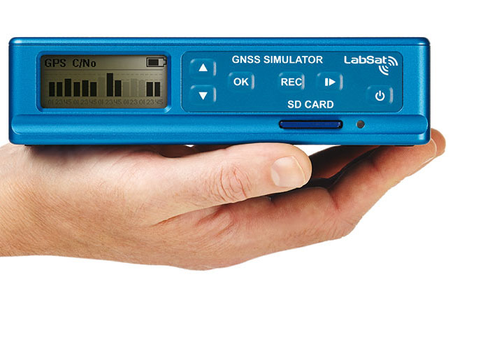
Racelogic LabSat3 simulator.
In order to help companies test for this problem, Racelogic has generated simulated RF data for June 29 and 30, starting 15 minutes before midnight. “We have two sets of files. One set contains BeiDou only signals and the other contains a combination of BeiDou and GPS signals,” Sampson said. “Note that on some of the receivers we have tested, when GPS is being tracked as well, the GPS leap-second message overrides the one coming from BeiDou and applies the leap second correctly.”
The scenarios are compatible with Racelogic’s LabSat3 triple constellation simulator, which is available on a free 15-day loan or can be purchased from Racelogic.
The German Galileo test and development infrastructure GATE has been recertified to serve as a Galileo open‐air test laboratory, for receiver integrity testing (RAIM) for safety‐of‐life (SoL) applications, and for Galileo SIS ICD conformance of signal characteristics and signal quality.
The GATE facility, in Berchtesgaden, is operated by IFEN GmbH. Certification was conducted by TÜV SÜD, an international service corporation focusing on consulting, testing, certification and training.
GATE consists of eight transmitting stations that emit Galileo signals in the GATE test area in Berchtesgaden, as well as two monitoring stations that receive and process these signals.
For application tests, it is essential for GATE to provide constant Galileo specifications for tests, including position accuracy, signal spectrum and navigation data. This is necessary for both test types: tests with the eight “GATE satellites” only and tests with simultaneously usage of the already-existing Galileo satellites in orbit.
The compliance to the specification was verified by the company NavCert GmbH from Braunschweig, Germany, in a recertification of the GATE test bed. Compared to a full certification, taking place every three years, a recertification only verifies the compliance to the specification by the use of random inspections though tests in GATE.
The recertification also includes an audit of the operation processes of the operating company IFEN GmbH. Here, the implementation and adherence to process procedures for GATE operation were verified. This includes questions such as whether a sufficiently technical skilled team is available for operating GATE, if the performed application tests are documented in a reproducible way, and how the GATE team handles non‐conformances to the specification and improvements to the system.
With finalization of the recertification work, the GATE certificate was extended by TÜV SÜD to January 2016. Because of this, GATE customers can rely on the independent verification of the GATE test and development environment for upcoming testing activities, IFEN said.
As an add‐on, customers of IFEN’s NavX‐NCS GNSS simulator benefit from the recertification by obtaining a confirmation from an independent organization (TÜV Süd), reassuring the functionality of GPS and Galileo signal characteristics and signal quality as per SIS ICD, IFEN said.
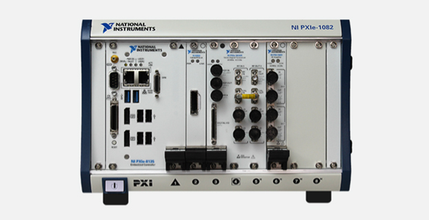
M3 Systems is now offering the StellaNGC multi-constellation GNSS simulator based on the National Instruments (NI) vector signal transceiver.
The simulator is designed for the testing of satellite navigation receivers for GPS, GLONASS, Galileo, and EGNOS/WAAS. It is designed to improve performance, scalability, and versatility, and reduce cost over existing navigation test solutions.
GNSS is the predominant technology today for navigation and outdoor positioning. However, given the weakness of GNSS signals, receiver performance is often affected by interference from the local environment and propagation channel conditions. Understanding the effects of this interference is of particular importance not only for existing GNSS signals but also for future signals that will appear with the deployment of new constellations such as Galileo.
To properly characterize receiver performance under varying conditions, the StellaGNC multi-constellation GNSS simulator provides signal generation, signal recording and replay, interference generation, signal and data processing, and complete analysis tools. The StellaNGC simulator is based on the NI vector signal transceiver in PXI for improved performance and full simulation capabilities. For record and playback only, a scaled-down version is also available based on the NI USRP (Universal Software Radio Peripheral). Both options were developed with NI LabVIEW and benefit from the performance and flexibility of the NI RF platform.
The simulator provides a scalable solution that allows easy signal additions through software upgrades, multi-frequency, processing extensions with the addition of FPGAs with NI FlexRIO, and an HDD extension for storage increase. Because the simulator is based on the open PXI standard, the hardware investment can also be extended to other applications, such as simulation, record and playback, or payload simulation.
TerraStar GNSS, a supplier of precision positioning services for land and near-shore applications, has established a base at Nottingham University’s GNSS Research and Applications Centre of Excellence (GRACE). GRACE operates operates under the auspices of its Institute of Engineering Surveying & Space Geodesy (IESSG).
TerraStar GNSS maintains and controls a worldwide network of more than 80 GPS and GLONASS DGNSS reference stations and associated control centers on behalf of a diverse range of users. Under the collaborative venture, TerraStar GNSS will contribute and have access to GRACE’s support facilities. These include customized incubation units, project offices, state-of-the-art test equipment, secure research and development laboratories, and dedicated training suites.
Expected projects include joint research and development of new GNSS-type solutions, in addition to provision of support for continued commercial exploitation of academic research endeavors. Also available will be mutual access to general geospatial expertise consistent with TerraStar GNSS’ present capability of providing year-round meter and decimeter-levels of precision for both land and aerial survey applications using software and a series of advanced purpose-designed integrated receivers.
Headed by General Manager Gary Wilcock, TerraStar GNSS’s new base facilities are at Office A03, The Nottingham Geospatial Building, University of Nottingham Innovation Park, Triumph Road, Nottingham NG7 2TU, UK.
The Galileo Test and Development Environment (GATE) in Berchtesgaden, Germany, officially opened on February 4. The system operator, IFEN GmbH of Poing, Germany, jointly with the German Federal Minister of Transport, Building and Urban Development, announced the opening for use by commercial and organizational entities seeking to test equipment with the coming Galileo signals. GATE was developed on behalf of the German Aerospace Center (DLR) with funding by the German Federal Ministry of Economics and Technology.
The test area extends across a valley of approximately 65 square kilometers, south-east of Munich, where antennae atop surrounding peaks broadcast the various Galileo signals. Technical details and specifications of the test environment are at www.gate-testbed.com.
GATE has completed its signal upgrade phase according to the latest version of the European Space Agency’s Galileo Signal-In-Space (SIS) Interface Control Document (ICD) and the European GNSS Agency’s Public Galileo Open Service (OS) ICD. The GATE infrastructure is capable of transmitting the Galileo OS, the Galileo Safety-of-Life (SoL) Service (functional), the Galileo Commercial Service (CS), and a Galileo Public Regulated Service (PRS) dummy signal.
The GATE system upgrade has been further extended to also support user integrity testing. GATE can simulating simple alarm-triggering events on the system/satellite level, supporting GPS and GATE/Galileo dual-constellation receiver-autonomous integrity monitoring (RAIM), individual user integrity test scenarios, and tests of receivers with different RAIM functionalities.
The next step will be certification of the GATE test infrastructure as an officially accredited open-air test infrastructure to perform the necessary tests needed for the process to certify Galileo SoL equipment.
Günter Heinrichs, head of customer applications and business development for IfEN GmbH, described the goals and capabilities of GATE in a 2007 GPS World article. He gave an update on developments in a 2009 video interview. A recent simulation of emergency response scenarios using the Galileo signal is described at Galileo to the Rescue.
By Axel van den Berg, Tom Willems, Graham Pye, and Wim de Wilde, Septentrio Satellite Navigation, Richard Morgan-Owen, Juan de Mateo, Simone Scarafia, and Martin Hollreiser, European Space Agency
A fully stand-alone, multi-frequency, multi-constellation receiver unit, the TUR-N can autonomously generate measurements, determine its position, and compute the Galileo safety-of-life integrity.
Development of a reference Galileo Test User Receiver (TUR) for the verification of the Galileo in-orbit validation (IOV) constellation, and as a demonstrator for multi-constellation applications, has culminated in the availability of the first units for experimentation and testing. The TUR-N covers a wide range of receiver configurations to demonstrate the future Galileo-only and GPS/Galileo combined services:
Galileo single- and dual-frequency Open Services (OS)
Galileo single- and dual-frequency safety-of-life services (SoL), including the full Galileo navigation warning algorithms
Galileo Commercial Service (CS), including tracking and decoding of the encrypted E6BC signal
GPS/SBAS/Galileo single- and dual- frequency multi-constellation positioning
Galileo single- and dual-frequency differential positioning.
Galileo triple-frequency RTK.
In parallel, a similar test user receiver is specifically developed to cover the Public Regulated service (TUR-P). Without the PRS components and firmware installed, the TUR-N is completely unclassified.
Main Receiver Unit
The TUR-N receiver is a fully stand-alone, multi-frequency, multi-constellation receiver unit. It can autonomously generate measurements, determine its position, and compute Galileo safety-of-life integrity, which is output in real time and/or stored internally in a compact proprietary binary data format.
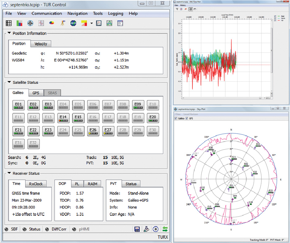
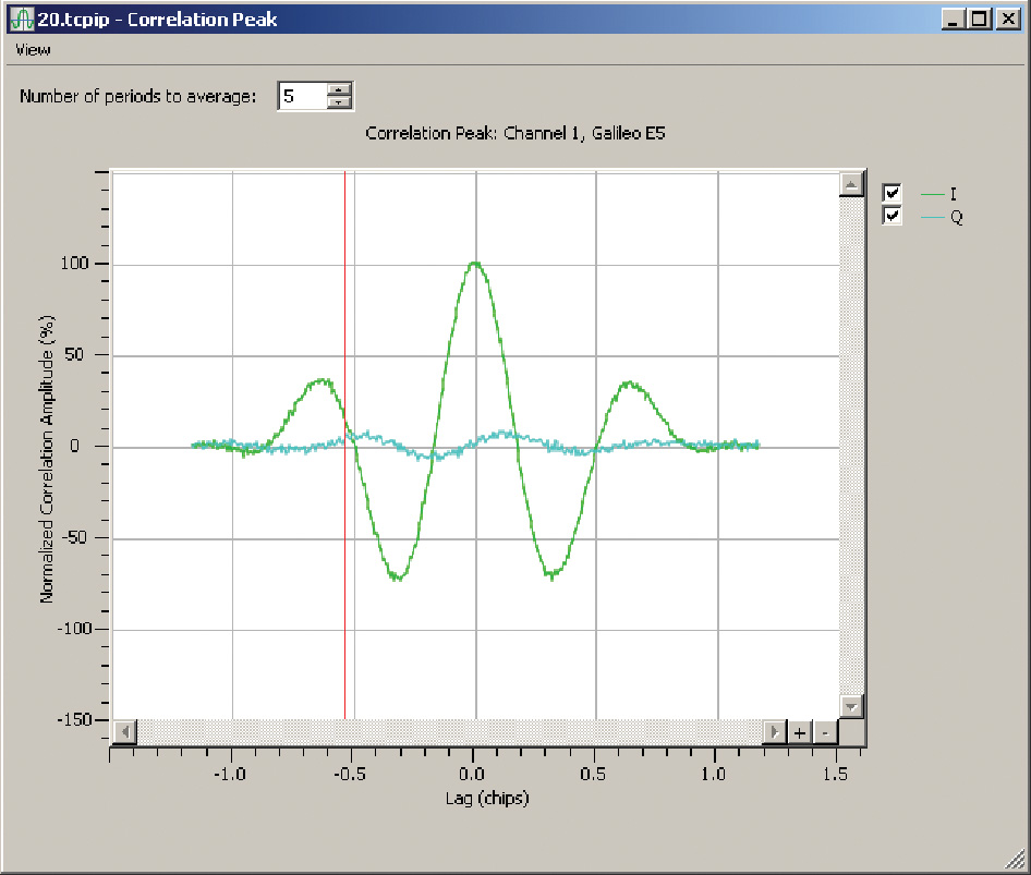
The receiver configuration is fully flexible via a command line interface or using the dedicated graphical user interface (GUI) for monitoring and control. With the MCA GUI it is also possible to monitor the receiver operation (see Figure 1), to present various real-time visualizations of tracking, PVT and integrity performances, and off-line analysis and reprocessing functionalities. Figure 2 gives an example of the correlation peak plot for an E5 AltBOC signal.
FIGURE 1. TUR-N control screen.FIGURE 2. E5 AltBOC correlation peak.
A predefined set of configurations that map onto the different configurations as prescribed by the Test User Segment Requirements (TUSREQ) document is provided by the receiver.
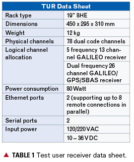
The unit can be included within a local network to provide remote access for control, monitoring, and/or logging, and supports up to eight parallel TCP/IP connections; or, a direct connection can be made via one of the serial ports.
Receiver Architecture
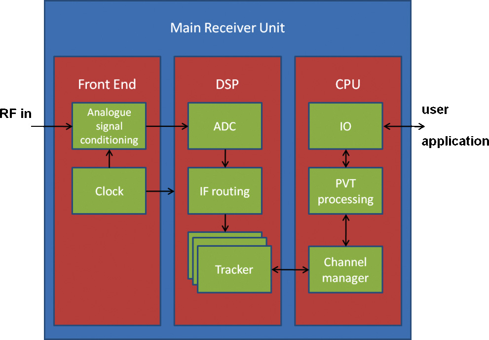
The main receiver unit consists of three separate boards housed in a standard compact PCI 19-inch rack. See Figure 3 for a high-level architectural overview.
FIGURE 3. Receiver architecture.
A dedicated analog front-end board has been developed to meet the stringent interference requirements. This board contains five RF chains for the L1, E6, E5a/L5, E5b, and E5 signals. Via a switch the E5 signal is either passed through separate filter paths for E5a and E5b or via one wide-band filter for the full E5 signal. The front-end board supports two internal frequency references (OCXO or TCXO) for digital signal processing (DSP).
The DSP board hosts three tracker boards derived from a commercial dual-frequency product family. These boards contain two tracking cores, each with a dedicated fast-acquisition unit (FAU), 13 generic dual-code channels, and a 13-channel hardware Viterbi decoder. One tracking core interacts with an AES unit to decrypt the E6 Commercial Service carrier; it has a throughput of 149 Mbps.
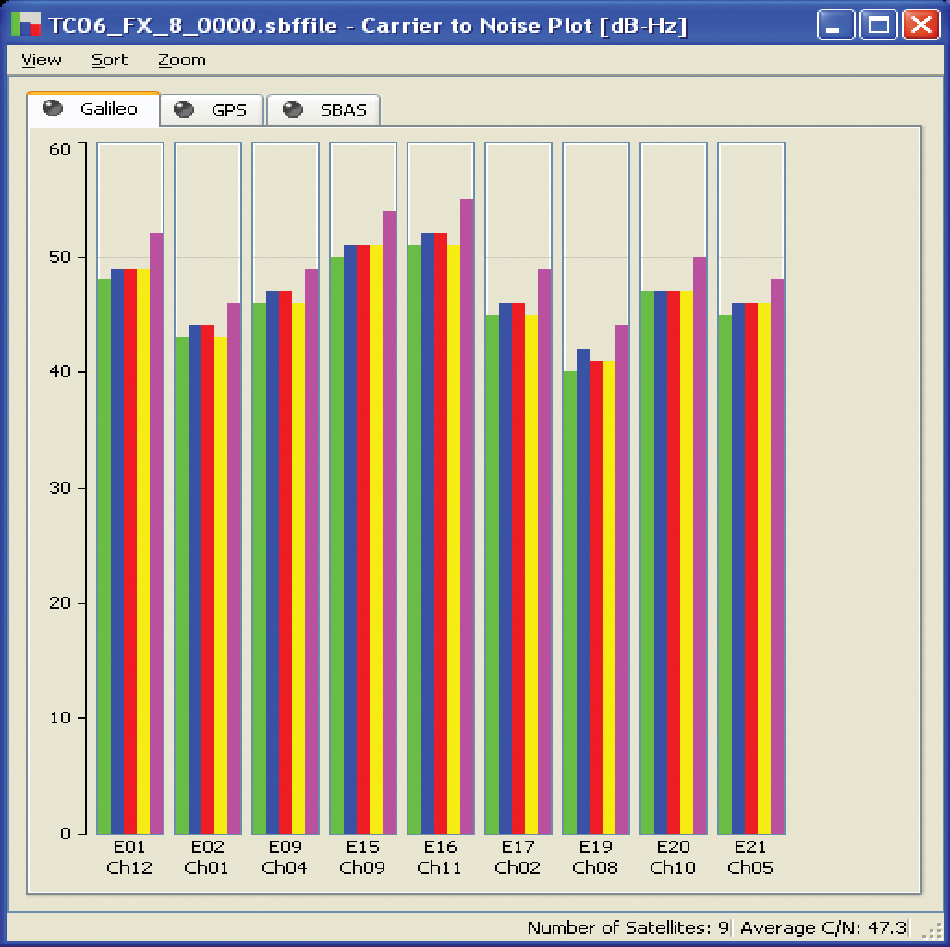
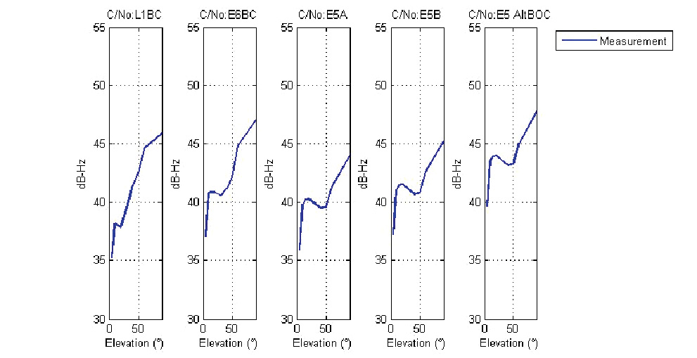
Each FAU combines a matched filter with a fast Fourier transform (FFT) and can verify up to 8 million code-frequency hypotheses per second. Each of the six tracker cores can be connected with one of the three or four incoming IF streams. To simplify operational use of the receiver, two channel-mapping files have been defined to configure the receiver either for a 5-frequency 13-channel Galileo receiver, or for a dual-frequency 26-channel Galileo/GPS/SBAS receiver. Figure 4 shows all five Galileo signal types being tracked for nine visible satellites at the same time.
FIGURE 4. C/N0 plot with nine satellites and all five Galileo signal types: L1BC (green), E6BC (blue), E5a (red), E5b (yellow), and E5 Altboc (purple).
The receiver is controlled using a COTS CPU board that also hosts the main positioning and integrity algorithms. The processing power and available memory of this CPU board is significantly higher than what is normally available in commercial receivers. Consequently there is no problem in supporting the large Nequick model used for single-frequency ionosphere correction, and achieving the 10-Hz update rate and low latency requirements when running the computationally intensive Galileo integrity algorithms. For commercial receivers that are normally optimized for size and power consumption, these might prove more challenging.
The TUR project included development of three types of Galileo antennas:
a triple-band (L1, E6, E5) high-end antenna for fixed base station applications including a choke ring;
a triple-band (L1, E6, E5) reference antenna for rover applications;
a dual-band (L1, E5b) aeronautic antenna for SOL applications
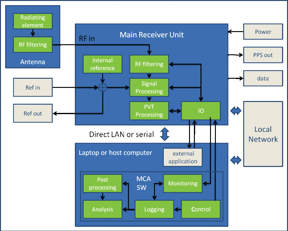
Figure 5 shows an overview of the main interfaces and functional blocks of the receiver, together with its antenna and a host computer to run the MCA software either remotely or locally connected.
FIGURE 5. TUR-N with antenna and host computer.
Receiver Verification
Currently, the TUR-N is undergoing an extensive testing program. In order to fully qualify the receiver to act as a reference for the validation of the Galileo system, some challenges have to be overcome. The first challenge that is encountered is that the performance verification baseline is mainly defined in terms of global system performance. The translation of these global requirements derived from the Galileo system requirements (such as global availability, accuracy, integrity and continuity, time-to-first/precise-fix) into testable parameters for a receiver (for example, signal acquisition time, C/N0 versus elevation, and so on) is not trivial. System performances must be fulfilled in the worst user location (WUL), defined in terms of dynamics, interference, and multipath environment geometry, and SV-user geometry over the Galileo global service area.
A second challenge is the fact that in the absence of an operational Galileo constellation, all validation tests need to be done in a completely simulated environment. First, it is difficult to assess exactly the level of reality that is necessary for the various models of the navigation data quality, the satellite behaviour, the atmospheric propagation effects, and the local environmental effects. But the main challenge is that not only the receiver that is being verified, also the simulator and its configuration are an integral part of the verification. It is thus an early experience of two independent implementations of the Galileo signal-in-space ICD being tested together. At the beginning of the campaign, there was no previously demonstrated or accepted test reference.
Only the combined efforts of the various receiver developments benchmarked against the same simulators together with pre-launch compatibility tests with the actual satellite payload and finally IOV and FOC field test campaigns will ultimately validate the complete system, including the Galileo ground and space segments together with a limited set of predefined user segment configurations. (Previously some confidence was gained with GIOVE-A/B experimental satellites and a breadboard adapted version of TUR-N). The TUR-N was the first IOV-compatible receiver to be tested successfully for RF compatibility with the Galileo engineering model satellite payload.
Key Performances
Receiver requirements, including performance, are defined in the TUSREQ document.
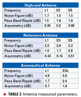
Antenna and Interference. A key TUSREQ requirement focuses on receiver robustness against interference. It has proven quite a challenge to meet the prescribed interference mask for all user configurations and antenna types while keeping many other design parameters such as gain, noise figure, and physical size in balance. For properly testing against the out-of-band interference requirements, it also proved necessary to carefully filter out increased noise levels created by the interference signal generator.
Table 2 gives an overview of the measured values for the most relevant Antenna Front End (AFE) parameters for the three antenna types. Note: Asymmetry in the AFE is defined as the variation of the gain around the centre frequency in the passband. This specification is necessary to preserve the correlation peak shape, mainly of the PRS signals.
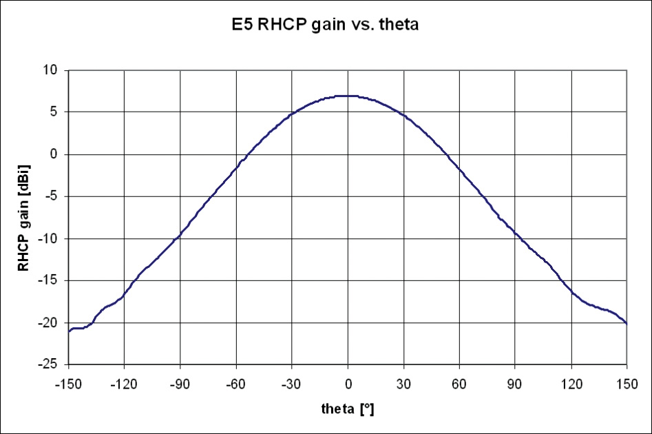
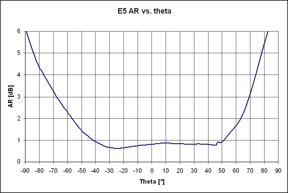
The gain for all antenna front ends and frequencies is around 32 dB. Figures 6 and 7 give an example of the measured E5 RHCP radiating element gain and axial ratio against theta (the angle of incidence with respect to zenith) for the high-end antenna-radiating element. Thus, elevation from horizontal is 90-theta.
UERE Performance. As part of the test campaign, TUR performance has been measured for user equivalent range error (UERE) components due to thermal noise and multipath.
TUSREQ specifies the error budget as a function of elevation, defined in tables at the following elevations: 5, 10, 15, 20, 30, 40, 50, 60, 90 degrees. The elevation dependence of tracking noise is immediately linked to the antenna gain pattern; the antenna-radiating element gain profiles were measured on the actual hardware and loaded to the Radio Frequency Constellation Simulator (RFCS), one file per frequency and per antenna scenario. The RFCS signal was passed through the real antenna RF front end to the TUR. As a result, through the configuration of RFCS, real environmental conditions (in terms of C/N0) were emulated in factory.
The thermal noise component of the UERE budget was measured without multipath being applied, and interference was allowed for by reducing the C/N0 by 3 dB from nominal. Separately, the multipath noise contribution was determined based on TUSREQ environments, using RFCS to simulate the multipath (the multipath model configuration was adapted to RFCS simulator multipath modeling capabilities in compliance with TUSREQ). To account for the fact that multipath is mostly experienced on the lower elevation satellites, results are provided with scaling factors applied for elevation (“weighted”), and without scaling factors (“unweighted”). In addition, following TUSREQ requirements, a carrier smoothing filter was applied with 10 seconds convergence time.
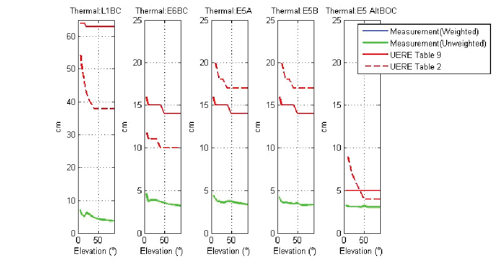
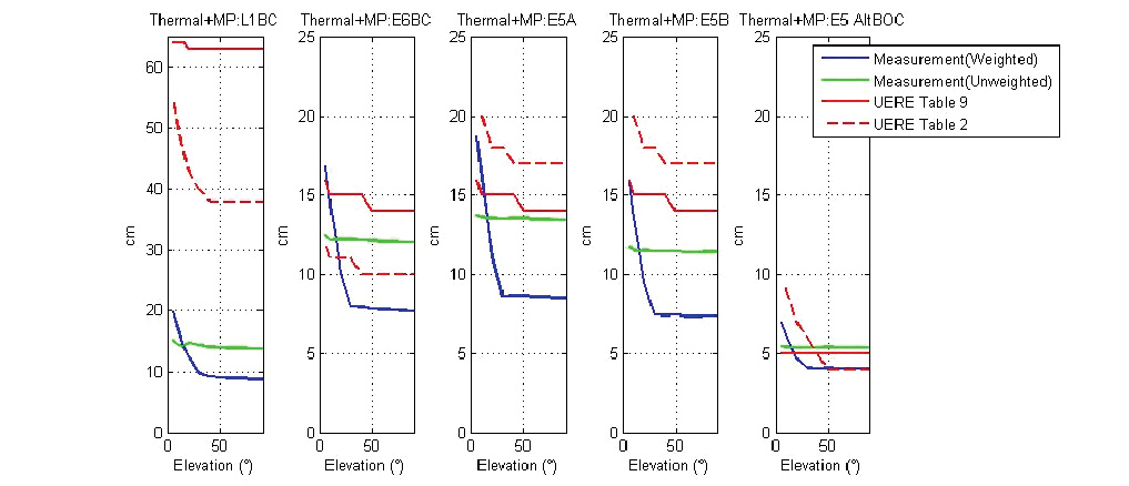
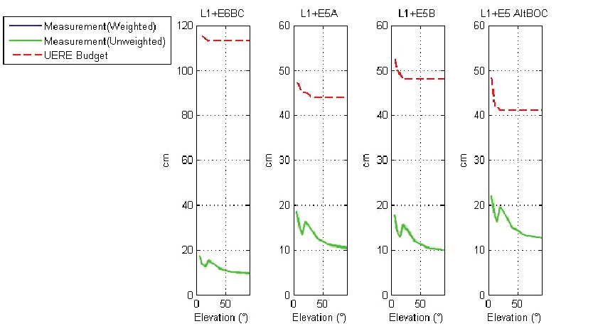
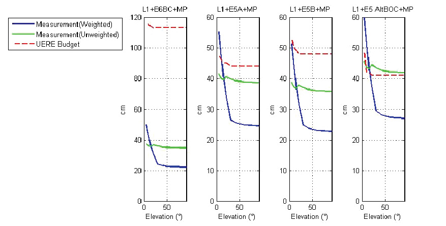
Figure 8 shows the C/N0 profile from the reference antenna with nominal power reduced by 3 dB. Figure 9 shows single-carrier thermal noise performance without multipath, whereas Figure 10 shows thermal noise with multipath. Each of these figures includes performance for five different carriers: L1BC, E6BC, E5a, E5b, and E5 AltBOC, and the whole set is repeated for dual-frequency combinations (Figure 11 and Figure 12).
FIGURE 8. Reference antenna, power nominal-3 dB, C/N0 profile.FIGURE 9. Reference antenna, power nominal-3 dB, thermal noise only, single frequency.FIGURE 10. Reference antenna, power nominal-3 dB, thermal noise with multipath, single frequency.FIGURE 11. Reference antenna, power nominal-3 dB, thermal noise only, dual frequency.FIGURE 12. Reference antenna, power nominal-3 dB, thermal noise with multipath, dual frequency.
The plots show that the thermal noise component requirements are easily met, whereas there is some limited non-compliance on noise+multipath (with weighted multipath) at low elevations. The tracking noise UERE requirements on E6BC are lower than for E5a, due to assumption of larger bandwidth at E6BC (40MHz versus 20MHz). Figures 9 and 10 refer to UERE tables 2 and 9 of TUSREQ. The relevant UERE requirement for this article is TUSREQ table 2 (satellite-only configuration). TUSREQ table 9 is for a differential configuration that is not relevant here.
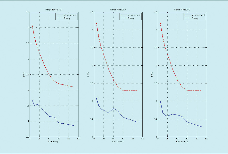
UERRE Performance. The complete single-frequency range-rate error budget as specified in TUSREQ was measured with the RFCS, using a model of the reference antenna. The result in Figure 13 shows compliance.
FIGURE 13. UERRE measurements.FIGURE 14. L1 GPS CA versus E5 AltBOC position accuracy (early test result).
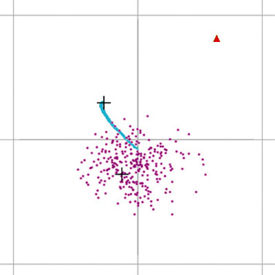
Position Accuracy. One of the objectives of the TUR-N is to demonstrate position accuracy. In Figure 14 an example horizontal scatter plot of a few minutes of data shows a clear distinction between the performances of two different single-frequency PVT solutions: GPS L1CA in purple and E5AltBOC in blue. The red marker is the true position, and the grid lines are separated at 0.5 meters. The picture clearly shows how the new E5AltBOC signal produces a much smoother position solution than the well-known GPS L1CA code. However, these early results are from constellation simulator tests without the full TUSREQ worst-case conditions applied.
FIGURE 14. L1 GPS CA versus E5 AltBOC position accuracy (early test result).
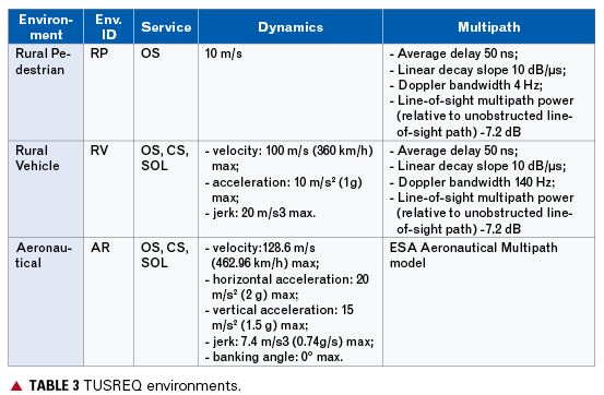
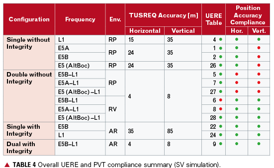
The defined TUSREQ user environments, the basis for all relevant simulations and tests, are detailed in Table 3. In particular, the rural pedestrian multipath environment appears to be very stringent and a performance driver.
This was already identified at an early stage during simulations of the total expected UERE and position accuracy performance compliance with regard to TUSREQ, summarized in Table 4, and is now confirmed with the initial verification tests in Figure 10. UERE (simulated) total includes all other expected errors (ionosphere, troposphere, ODTS/BGD error, and so on) in addition to the thermal noise and multipath, whereas the previous UERE plots were only for selected UERE components. The PVT performance in the table is based on service volume (SV) simulations.
The non-compliances on position accuracy that were predicted by simulations are mainly in the rural pedestrian environment. According to the early simulations:
E5a and E5b were expected to have 43-meter vertical accuracy (instead of 35-meter required).
L1/E5a and L1/E5b dual-frequency configurations were expected to have 5-meter horizontal, 12-meter vertical accuracy (4 and 8 required).
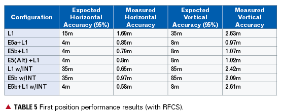
These predictions appear pessimistic related to the first position accuracy results shown in Table 5. On single frequency, the error is dominated by ionospheric delay uncertainty. These results are based on measurements using the RFCS and modeling the user environment; however, the simulation of a real receiver cannot be directly compared to service-volume simulation results, as a good balance between realism and worst-case conditions needs to be found. Further optimization is needed on the RFCS scenarios and on position accuracy pass/fail criteria to account for DOP variations and the inability to simulate worst environmental conditions continuously.
Further confirmations on Galileo UERE and position accuracy performances are expected after the site verifications (with RFCS) are completed, and following IOV and FOC field-test campaigns.
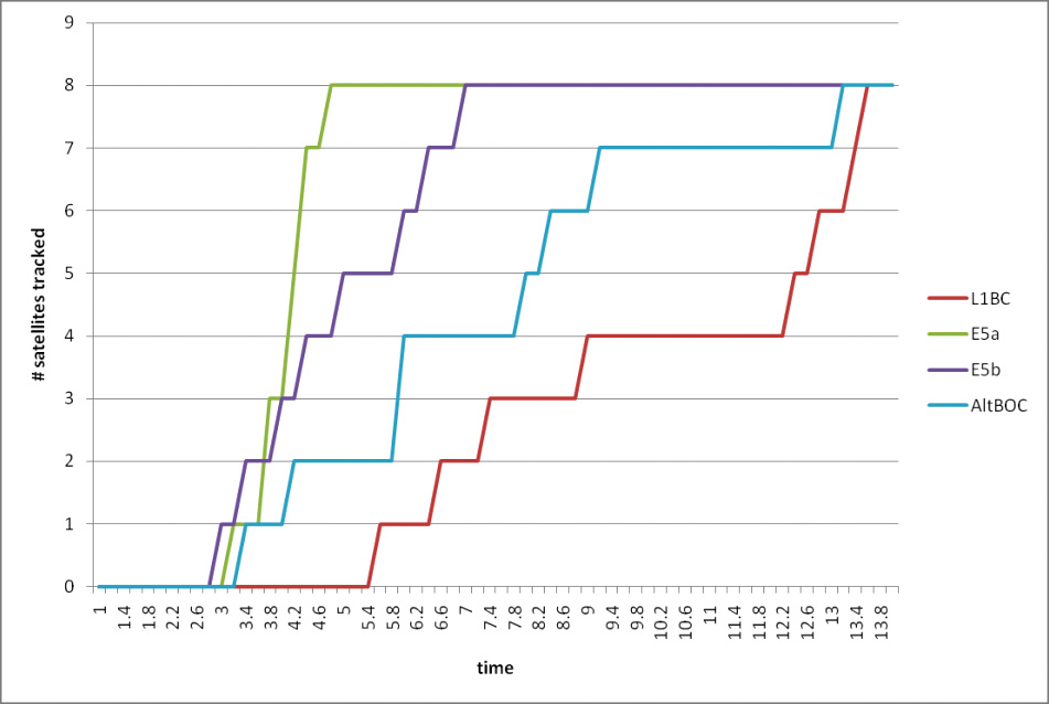
Acquisition. Figure 15 gives an example of different signal-acquisition times that can be achieved with the TUR-N after the receiver boot process has been completed. Normally, E5 frequencies lock within 3 seconds, and four satellites are locked within 10 seconds for all frequencies. This is based on an unaided (or free) search using a FAU in single-frequency configurations, in initial development test without full TUSREQ constraints.
FIGURE 15. Unaided acquisition performance.
When a signal is only temporarily lost due to masking, and the acquisition process is still aided (as opposed to free search), the re-acquisition time is about 1 second, depending on the signal strength and dynamics of the receiver. When the PVT solution is lost, the aiding process will time out and return to free search to be robust also for sudden user dynamics.
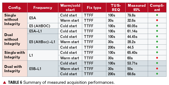
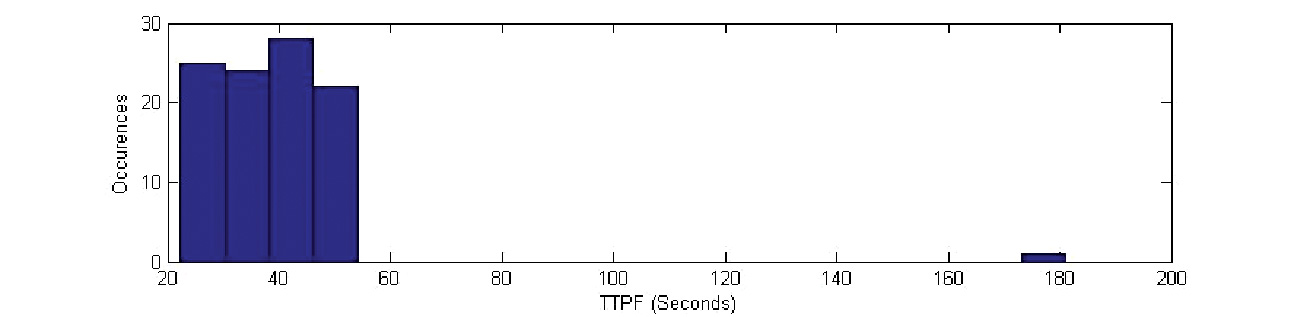
More complete and detailed time-to-first-fix (TTFF) and time-to-precise-fix (TTPF), following TUSREQ definitions, have also been measured.
In cold start the receiver has no prior knowledge of its position or the navigation data, whereas in warm start it already has a valid ephemeris in memory (more details on start conditions are available in TUSREQ). Table 6 shows that the acquisition performances measured are all compliant to TUSREQ except for warm start in E5a single frequency and in the integrity configurations. However, when the navigation/integrity message recovery time is taken off the measurement (as now agreed for updated TUSREQ due to message limitations), these performances also become compliant.
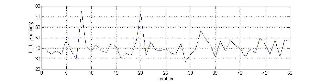
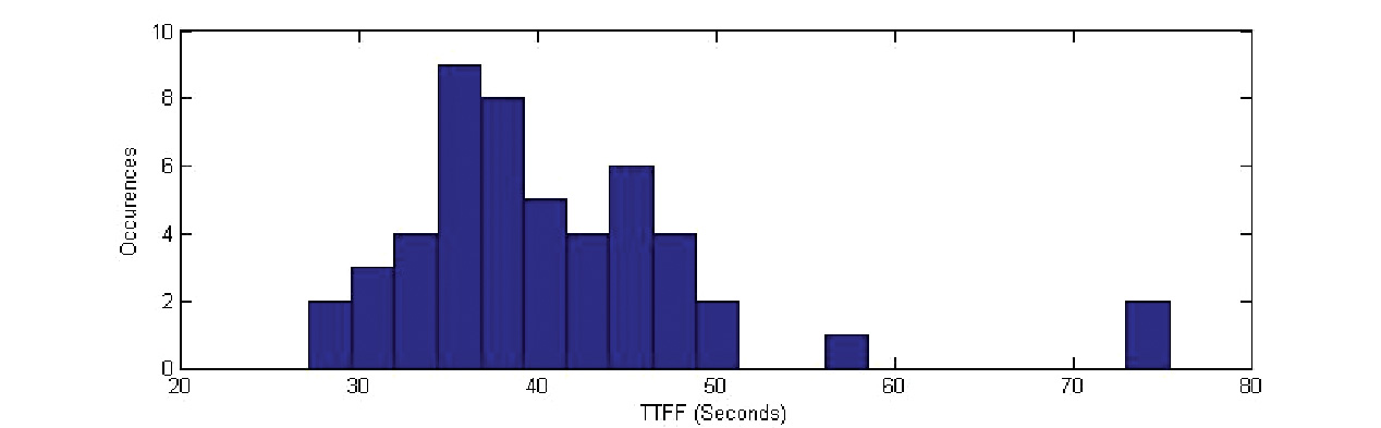
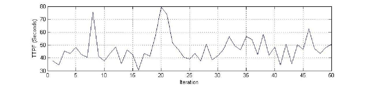
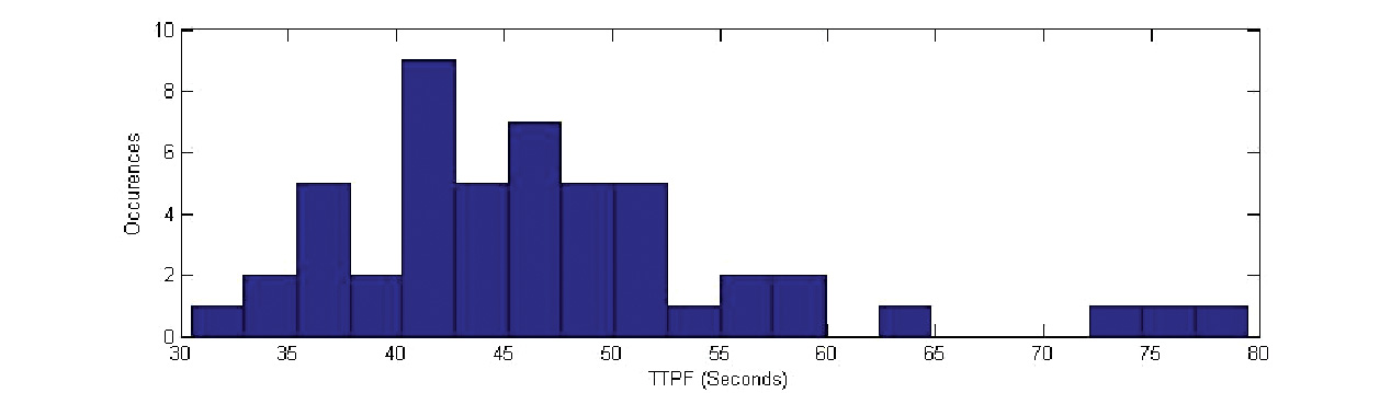
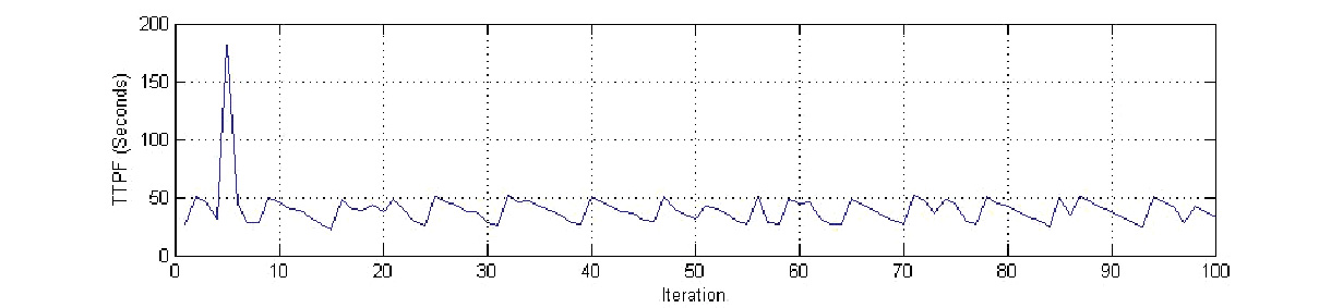
Specific examples of statistics gathered are shown in figures 16–21, these examples being for dual-frequency (E5b+L1) with integrity configuration. The outliers, being infrequent results with high acquisition times, are still compliant with the maximum TTFF/TTPF requirements, but are anyway under further investigation.
FIGURE 16. TTFF cold-start performance, dual frequency with integrity E5b+L1.FIGURE 17. TTFF cold-start distribution, dual frequency with integrity E5b+L1.FIGURE 18. TTPF cold-start performance, dual frequency with integrity E5b+L1.FIGURE 19. TTPF cold-start distribution, dual frequency with integrity E5b+L1.FIGURE 20. TTFF warm-start performance, dual frequency with integrity E5b+L1.FIGURE 21. TTFF warm-start distribution, dual frequency with integrity E5b+L1,
Integrity Algorithms. The Galileo SoL service is based on a fairly complex processing algorithm that determines not only the probability of hazardous misleading information (PHMI) based on the current set of satellites used in the PVT computation (HPCA), but also takes into consideration the PHMI that is achieved when one of the satellites used in the current epoch of the PVT computation is unexpectedly lost within the following 15 seconds. PHMI is computed according to alarm limits that are configurable for different application/service levels. These integrity algorithms have been closely integrated into the PVT processing routines, due to commonality between most processing steps.
Current test results of the navigation warning algorithm (NWA) indicate that less than 10 milliseconds of processing time is required for a full cycle of the integrity algorithms (HPCA+CSPA) on the TUR-N internal CPU board. Latency of the availability of the integrity alert information in the output of the receiver after it was transmitted by the satellite has been determined to be below 400 milliseconds. At a worst-case data output rate of 10 Hz this can only be measured in multiples of 100 millisecond periods. The total includes 100 milliseconds of travel time of the signal in space and an estimated 250 milliseconds of internal latency for data-handling steps as demodulation, authentication, and internal communication to make the data available to the integrity processing.
Conclusions
The TUR-N is a fully flexible receiver that can verify many aspects of the Galileo system, or as a demonstrator for Galileo/GPS/SBAS combined operation. It has a similar user interface to commercial receivers and the flexibility to accommodate Galileo system requirements evolutions as foreseen in the FOC phase without major design changes.
The receiver performance is in general compliant with the requirements. For the important safety-of-life configuration, major performance requirements are satisfied in terms of acquisition time and position accuracy.
The receiver prototype is currently operational and undergoing its final verification and qualification, following early confirmations of compatibility with the RFCS and with the Galileo satellite payload.
AURORA BOREALIS seen from Churchill, Manitoba, Canada. Ionospheric scintillation research can benefit from this new method. (Photo: Aiden Morrison)Photo: Canadian Armed Forces
By Aiden Morrison, University of Calgary
Two broad user groups will find important consequences in this article:
Time synchronization and test equipment manufacturers, whose GPS-disciplined oscillators have excellent long-term performance but short- to medium-term behavior limited by the quality, and therefore cost, of the integrated quartz device. This article portends a family of devices delivering oven-controlled crystal oscillator (OCXO) performance down to the 10-millisecond level, with an oscillator costing pennies, rather than tens or hundreds of dollars. Applications include ionospheric scintillation research (above).
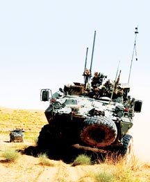
High-performance receiver manufacturers who design products for high-dynamic or high-vibration environments (see cover) where the contribution of phase noise from the local oscillator to velocity error cannot be ignored. In these areas, the strategy outlined here would produce equipment that can perform to higher specifications with the same or a lower-cost oscillator.
The trade-off requires two tracking channels per satellite signal, but this should not pose a problem. At ION GNSS 2009, manufacturers showed receivers with 226 tracking channels. There are currently only 75 live signals in the sky, including all of GPSL1/L2/L5 and GLONASS L1/L2. — Gérard Lachapelle
If the channel data within a GNSS receiver is handled in an effective manner, it is possible to form meaningful estimates of the local-oscillator phase deviations on timescales of 10 milliseconds (ms) or less. Moreover, if certain criteria are met, these estimates will be available with related uncertainties similar to the deviations produced by a typical oven-controlled crystal oscillator (OCXO). The processing delay required to form this estimate is limited to between 10 and 20 ms. In short, it becomes possible in near-real-time to remove the majority of the phase noise of a local oscillator that possesses short-term instability worse than an OCXO, using standalone GNSS. This represents both a new method to accurately determine the Allan deviation of a local oscillator at time scales previously impractical to assess using a conventional GNSS receiver, and the potential for the reduction in observable Doppler uncertainty at the output of the receiver, as well as ionospheric scintillation detection not reliant on an expensive local OCXO.
Concept. Inside a typical GNSS receiver, the estimate of the error in the local oscillator is formed as a component of the navigation solution, which is in turn based on the output of each satellite-tracking channel propagating its estimate of carrier and code measurements to a common future point. While this method of ensuring simultaneous measurements is necessary, it regrettably limits the resolution with which the noise of the local oscillator can be quantified, due to the scaling of non-simultaneous samples of local oscillator noise through the measurement propagation process. To bypass these shortcomings requires a method of coherently gathering information about the phase change in the local oscillator across all available satellite signals: to use the same samples simultaneously for all satellites in view to estimate the center-point phase error common across the visible constellation.
To explain how this is feasible, we must first understand the limitations imposed by the conventional receiver architecture, with respect to accurately estimating short-term oscillator behavior, and subsequently to determine the potential pitfalls of the proposed modifications, including processing delays needed for bit wipe-off, expected observation noise, and user dynamics effects.
Typical Receiver Shortfalls
In a typical receiver, while information about local time offset and local oscillator frequency bias may be recovered, information about phase noise in the local oscillator is distorted and discarded, as a consequence of scaling non-simultaneous observations to a common epoch.
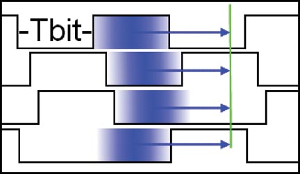
As shown in FIGURE 1, coherent summation intervals in a receiver are used to approximate values of the phase error, including oscillator phase, measured at the non-simultaneous interval centrers in each channel, which are then propagated to a common navigation solution epoch. Each channel will intrinsically contain a partially overlapping midpoint estimate of oscillator noise over the coherent summation interval that will then be scaled by the process of extrapolation. As these estimates are scaled and partially overlapping, they do not make optimal use of the information known about the effects of the local oscillator, and form a poor basis for estimating the contributions of this device to the uncertainty in the channel measurements. As shown in Figure 1, the phase error measured in each channel will be distorted by an over unity scaling factor.
FIGURE 1. Propagation and scaling of phase estimates within a typical receiver.
Depending on implementation decisions made by the designers of a given GNSS system, the average value of the propagation interval relative to the bit period will have different expected values. Assuming the destination epoch is the immediate end of the furthest advanced (most delayed) satellite bitstream, and that integration is carried out over full bit periods, the minimum propagation interval for this satellite would be ½-bit period.
For the average satellite however, the propagation delay would be this ½-bit period plus the mean skew between the furthest satellite and the bitstreams of other space vehicles. Ignoring further skew effects due to the clock errors within the satellites, which are typically limited well below the ms level, the skew between highest and lowest elevation GPS satellites for a user on the surface of earth would be approximately 10 ms. The average value of this skew due to ranging change over orbit, assuming an even distribution of satellites in the sky at different elevation angles, would therefore be 5 ms.
Combining the minimum value of the skew interval with the minimum propagation interval of the most delayed satellite yields a total average propagation interval of 15 ms. In turn, this gives a typical scaling factor of 1.75, used from this point forward when referring to the effects of scaling this quantity.
Proposed Implementation
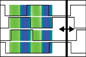
Overcoming limitations of a typical receiver requires recording the approximate bit-timing and history of each tracked satellite as well as a short segment of past samples. This retained data guarantees that the bit-period boundaries of the satellites will not pose an obstacle to forming common N-ms coherent periods between all visible satellites, over which simultaneous integration may proceed by wiping off bit transitions. Using this approach as shown in FIGURE 2, all available constellation signal power is used to estimate a single parameter, namely the epoch-to-epoch phase change in the local oscillator.
FIGURE 2. Common intervals over which to accurately estimate local oscillator phase changes.
Having viewed the existence of these common periods, it becomes evident that it is conceptually possible to form time-synchronized estimates of the phase contribution of the common system oscillator alternately across one N-ms time slice, then the next, in turn forming an unb
roken time series of estimates of the phase change of the system oscillator. Forming the difference between the adjacent discriminator outputs will provide the following information:
The ΔEps (change in the noise term in the local loop)
The ΔOsc (change in the phase of the local oscillator, the parameter of interest)
The ΔDyn (change in the untracked/residual of real and apparent dynamics of the local loop/estimator)
Noticing that term 1 may be considered entirely independent across independent PRNs (GPS, Galileo, Compass) or frequency channels (GLONASS), and that the value of term 3 over a 10-ms period is expected to be small over these short intervals, it becomes obvious that term 2 can be recovered from the available information. To determine the weighting for each satellite channel, the variance of the output of the discriminator is needed.
Performance Determination
To allow the realistic weighting of discriminator output deltas, it becomes desirable to estimate at very short time intervals the variance of the output of the phase discriminator. In the case of a 2-quadrant arctangent discriminator, this means one wishes to quantify the variance
Letting Q/I 5 Z, recall that if Y 5 aX then
Applying this to the variance of the input to the arctangent discriminator in terms of the in phase and quadrature accumulators, this would give
Rather than proceed with a direct evaluation from this point onward to determine the expression for the variance at the output of the discriminator, it is convenient to recognize that simpler alternatives exist since
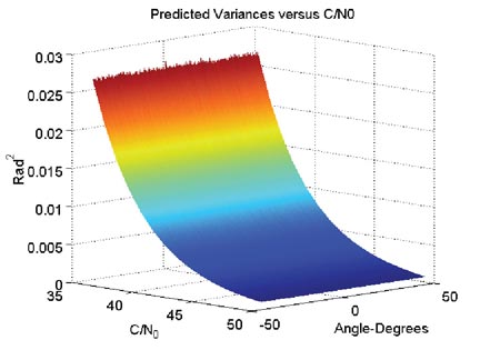
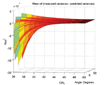
The implication is that since the slope of the arctangent transfer function is very nearly equal to 1 in the central, typical operating region, and universally less than 1 outside of this region, it is easy to recognize that the variance at the output of the arctangent discriminator is universally less than that at the input, and can be pessimistically quantified as the variance of the input, or σ2(Z). This assumption has been verified by simulation, its result shown in FIGURE 3, where the response has been shown after taking into account the effect of operating at a point anywhere in the range ±45 degrees. While the consequence of the simplification of the variance expression is an exaggeration of discriminator output variance, FIGURE 4 shows output variance is well bounded by the estimate, and within a small margin of error for strong signals.
FIGURE 3. Predicted variances at the output of the ATAN2 discriminator versus C/N0.FIGURE 4. Difference between actual and predicted variance at output of discriminator.
The gap between real and predicted output variance may also be narrowed in cases where Q>I by using a type of discriminator which interchanges Q and I in this case and adds an appropriate angular offset to the output as
Proceeding in this vein, the next required parameter is the normalized variance of the in-phase and quadrature arms.
The carrier amplitude A can be roughly approximated as
Resulting in a carrier power C
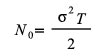
Further, the noise power is given as
Expressing bandwidth B as the inverse of the coherent integration time, and rearranging now gives noise density N0 as
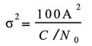
Combining this expression, and the one previously given for the carrier power C results in the following expression for the carrier to noise density ratio:
This latest expression can be rearranged to find the desired variance term. Assuming the 10-ms coherent integration time discussed earlier is used, this yields
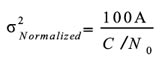
Normalizing for the carrier amplitude gives the normalized variance in terms of radians squared:
In any situation where the carrier is sufficiently strong to be tracked, it is likely that the carrier power term employed above can be gathered from the immediate I and Q values, ignoring the contribution of the noise term to its magnitude.
Oscillator Phase Effect. Determining the expected magnitude of the local oscillator phase deviation requires only three steps, assuming that certain criteria can be met. The first requirement is that the averaging times in question must be short relative to the duration, at which processes other than white phase and flicker phase modulation begin to dominate the noise characteristics of the oscillator. Typically the crossover point between the dominance of these processes and others is above 1 s in averaging interval length, when quartz oscillators are concerned. Since this article discusses a specific implementation interval of 10 ms within systems expected to be using quartz oscillators, it is reasonable to assume that this constraint will be met.
The second requirement is that the Allan deviation of the given system oscillator must be known for at least one averaging interval within the region of interest. Since the Allan deviation follows a linear slope of -1 with respect to averaging interval on a log-log scale within the white-phase noise region, this single value will allow an accurate prediction of the Allan deviation at any other point on the interval and, in turn, of the phase uncertainty at the 10 ms averaging interval level.
Letting σΔ(τ) represent the Allan deviation at a specific averaging interval, recall that this quantity is the midpoint average of the standard deviation of fractional frequency error over the averaging interval τ. Scaling this quantity by a frequency of interest results in the standard deviation of the absolute frequency error on the averaging interval:
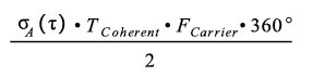
By integrating this average difference in frequency deviations over the coherent period of interest, one obtains a measure of the standard deviation in degrees, of a signal generated by this reference:
Note that the averaging interval τ must be identical to the coherent integration time.
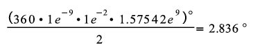
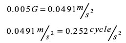
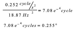
Turning to a practical example, if the oscillator in question has a 1 s Allan Deviation of 1 part per hundred billion (1 in 1011), a stability value between that of an OCXO and microcomputer compensated crystal oscillator (MCXO) standard, and shown to be somewhat pessimistic, this would scale linearly to be 1e-9 at a 10-ms averaging interval, under the previous assumption that the oscillator uncertainty is dominated by the white phase-noise term at these intervals. Also, for illustration purposes, if one assumes the carrier of interest to be the nominal GPS L1 carrier, the uncertainty in the local carrier replica due to the local oscillator over a 10-ms coherent integration time becomes
When stated in a more readily digested format, this represents roughly 15 centimeter/second in the line-of-sight velocity uncertainty. In an operating receiver, two additional factors modify this effect. The first is the previously discussed scaling effect that will tend to exaggerate this effect by a typical factor of 1.75, as previously discussed. The second factor is that this noise contribution is filtered by the bandwidth-limiting effects of the local loop filter, producing a modification to the noise affecting velocity estimates, as well as reduced information about the behaviour of the local oscillator.
Impact of Apparent Dynamics. When considering the error sources within the system, it is important to realize which individual sources of error will contribute to estimation errors, and which will not. One area of potential concern would appear to be the errors in the satellite ephemerides, encompassing both the satellite-orbit trajectory misrepresentation and the satellite clock error. While the errors in the satellite ephemerides are of concern for point positioning, they are not of consequence to this application, as the apparent error introduced by a deviation of the true orbit from that expressed in the broadcast orbital parameters does not affect the tracking of that satellite at the loop level.
Additionally, while the satellite clock will add uncertainty to the epoch-to-epoch phase change within each channel independently, the magnitude of this change is minimal relative to the contribution of uncertainty due to the variance at the output of the discriminator guaranteed by the low carrier-to-noise density ratio of a received GNSS signal. Since this contribution is uncorrelated between satellites and relatively small compared to other noise contributions affecting these measurements, even when compared to the soon-to-be-discontinued Uragan GLONASS satellites that had generally less stable onboard clocks, it is likely safe to ignore. When compared to the more stable oscillators aboard GPS or GLONASS-M satellites, it is a reasonable assumption that this will be a dismissible contribution to received signal-phase uncertainty change.
While atmospheric effects present an obstacle which will directly affect the epoch-to-epoch output of the discriminators, it is believed that under conditions that do not include the effects of ionospheric scintillation the majority of the contribution of apparent dynamics due to atmospheric changes will have a power spectral density (PSD) heavily concentrated below a fraction of 1 Hz. The consequence of this concentration is that the tracking loops will remove the vast majority of this contribution, and that the difference operator that will be applied between adjacent phase measurements, as in the case of dynamics, will nullify the majority of the remaining influence.
Impact of Real Dynamics. Real dynamics present constraints on performance, as do any tracking loop transients. For example, a low-bandwidth loop-tracking dynamics will have long-lasting transients of a magnitude significant relative to levels of local oscillator noise. For this reason it is necessary to adopt a strategy of using the epoch-to-epoch change in the discriminator as the figure of interest, as opposed to the absolute error-value output at each epoch. This can reasonably be expected to remove the vast majority of the effects of dynamics of the user on the solution.
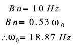
To validate this assumption under typical conditions calls for a short verification example. Assuming the use of a second-order phase-locked loop (PLL) for carrier tracking, with a 10-Hz loop bandwidth the effects of dynamics on the loop are given by these equations:
Letting Bn be 10 Hz, one can write
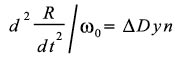
Recall that the dynamic tracking error in a second-order tracking loop is given by
Given the choices above, this would result in a constant offset of 0.00281 cycles, or 1.011 degrees of constant tracking error due to dynamics, following from the relation between line-of-sight acceleration and loop bandwidth to tracking error. Since this constant bias will be eliminated by the difference operator discussed earlier, it is necessary to examine higher order dynamics.
Further, if one used a coherent integration interval of 10 ms as assumed earlier, and let the dynamics of interest be a jerk of 1 g/s, this results in a midpoint average of 0.005 g on this interval:
Substituting this result into equation 16 produces the associated change in dynamic error over the integration interval, which is in this case:
This value will be kept in mind when evaluating capabilities of the estimation approach to determine when it will be of consequence. As the estimation process will be run after a short delay, an existing estimate of platform dynamics could form the basis of a smoothing strategy to reduce this dynamic contribution further.
Estimated Capabilities
In the absence of the influence of any unmodeled effects, the expected performance of this method is dependent on only the number of satellite observables and their respective C/N0 ratios. Across each of these scenarios we assume for simplicity’s sake that each satellite in view is received at a common C/N0 ratio and over a common integration period of 10 ms.
If the assumption of minimal dynamic influences is met, the situation at hand becomes one in which multiple measures of a single quantity are present, each containing independent (due to CDMA or FDMA channel separation) noise influences with a nearly zero mean. When one can express the available data form:
x[n] = R + w[n]
where x[n] is the nth channel discriminator delta which includes the desired measure of the local oscillator delta (R), as well as w[n], a strong, nearly white-noise component, there are multiple approaches for the estimation of R.
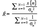
The straightforward solution to estimate R in this case is to use the predicted variances of each measure to serve as an inverse weighting to the contribution of each individual term, followed by normalization by the total variance, as expressed by
Now, since it is desired to bound the uncertainty of the estimate of R, the variance of this quantity should also be noted. This uncertainty can be determined as
To determine the performance of the estimation method for a given constellation configuration, with specific power levels and available carrier signals, it is necessary to utilize the predicted variances plotted in Figure 3 as inputs to equations 20 and 21. To provide numerical examples of the performance of this method, three scenarios span the expected range of performance.
Scenario 1 is intended to be char-acteristic of that visible to a single-freq-uency GPS user under slight attenuation. It is assumed that 12 single-frequency satellites are visible at a common C/N0 of 36 dB-Hz, yielding from the simulation curves a value for each channel of 0.0265 rad2. When substituted into equation 24, this predicts an estimation uncertainty of
This is a level of estimation uncertainty similar to that assumed to be intrinsic to the local oscillator in the previous section. The result implies that with this minimally powerful set of satellites, it becomes possible to quantify the behavior of the local oscillator with a level of uncertainty commensurate with the actual uncertainty in the oscillator over the 10 ms averaging interval.
Consequentially, this indicates that the Allan deviation of this system oscillator could be wholly evaluated under these conditions at any interval of 10 ms or longer. Further, if the system oscillator were in fact the less stable MCXO from the resource above, this estimate uncertainty would be significantly lower than the actual uncertainty intrinsic to the oscillator, providing an opportunity to “clean” the velocity measurements.
Scenario 2 is intended to be characteristic of a near future multi-constellation single-frequency receiver. It is assumed that eight satellites from three constellations are visible on a single frequency each, with a common C/N0 of 42 dB-Hz, yielding a value for each channel of 6.4e-3 rad2, leading to an estimation uncertainty of
Scenario 3 is intended to serve as an optimistic scenario involving a future multi-frequency, multi-constellation receiver. It is assumed that nine future satellites are available from each of three constellations, each with four independent carriers, all received at 45 dB-Hz, yielding a value for each channel of 3.2e-3 rad2, leading to an estimation uncertainty of
Application to Observations
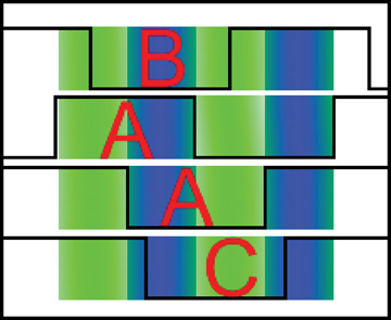
The theoretical benefit of subtracting these phase changes from the measurements of an individual loop prior to propagating that measurement to the common position solution epoch ranges from moderate to very high depending on the satellite timing skew relative to the solution point. The most beneficial scenario is total elimination of oscillator noise effects (within the uncertainty of the estimate), which is experienced in the special case (Case A, FIGURE 5), where the bit period of a given satellite falls entirely over two of the 10-ms subsections. The uncertainty would increase to 2x the level of uncertainty in the estimate in the special case (Case B) where the satellite bit period straddles one full 10-ms period and two 5-ms halves of adjacent periods, and would lie somewhere between 1 and 2 times the level of uncertainty for the general case where three subintervals are covered, yet the bit period is not centered (Case C).
FIGURE 5. Special cases of oscillator estimate versus bit-period alignment.
While the application to observations of the predicted oscillator phase changes between integration intervals does not appear immediately useful for high-end receiver users with the exception of those in high-vibration or scintillation-detection applications, it could be applied to consumer-grade receivers to facilitate the use of inexpensive system clocks while providing observables with error levels as low as those provided by much more expensive receivers incorporating ovenized frequency references.
Further Points
While the chosen coherent integration period may be lengthened to increase the certainty of the measurement from a noise averaging perspective, this modification risks degrading the usefulness of said measurement due to dynamics sensitivities. Additionally, as the coherent integration time is increased, the granularity with which the pre-propagation oscillator contribution may be removed from an individual loop will be reduced. While this may be useful in cases of very low dynamics where the system is intended to estimate phase errors in a local oscillator with high certainty, it would be of little use if one desires to provide low-noise observables at the output.
For this reason, it is recommended that increases in coherent integration time be approached with caution, and extra thought be given to use of dynamics estimation techniques such as smoothing, via use of the subsequent n-ms segment in the formation of the estimate of dynamics for the “current” segment. This carries the penalty of increased processing latency, but could greatly reduce dynamics effects by enabling their more reliable excision from the desired phase-delta measurements.
Acknowledgments
The author thanks his supervisors, Gerard Lachapelle and Elizabeth Cannon, and the Natural Sciences and Engineering Research Council of Canada, the Alberta Informatics Circle of Research Excellence, the Canadian Northern Studies Trust, the Association of Canadian Universities for Northern Studies, and Environment Canada for financial and logistical support.
AIDEN MORRISON is a Ph.D. candidate in the Position, Location, and Navigation (PLAN) Group, Department of Geomatics Engineering, Schulich School of Engineering at the University of Calgary, where he has developed a software-defined GPS/GLONASS receiver for his research.