GNSS researchers presented hundreds of papers at the 2023 Institute of Navigation (ION) GNSS+ conference, which took place Sept. 11-15, 2023, in Denver, Colorado, and virtually.
The following four papers focused on ways to combat GNSS jamming and spoofing. The papers are available at bit.ly/3UMAS13.
GPS World will be attending this year’s ION conference in Baltimore, Maryland on Sept. 16-20.
Photo: flashfilm / The Image Bank / Getty Images
Fault free integrity of urban driverless vehicles
For positioning in urban environments, systems can be integrated with an inertial navigation system (INS) to help provide continuous navigation through GNSS signal outages. Besides GNSS, another approach for positioning in urban environments is feature-matching. For example, light detection and ranging (lidar) can measure distances and angles for environmental features, such as local landmarks, which can then be associated with known feature locations stored in an onboard database.
This paper investigates how GNSS and INS, when augmented by lidar ranging from local landmarks, can offer safe navigation through a real-world urban environment under fault-free assumptions to achieve 100% availability of fault-free integrity, with requirements corresponding to maximum standard deviations between 0.05 m and
0.1 m in both lateral and longitudinal directions. The team determined which system elements and parameters are the most critical to urban navigation performance, including individual INS noise parameter specifications, average vehicle speed, kinematic constraints, landmark density, integrity requirements and the effects of velocity updates.
The team simulated GNSS availability along a 9 km urban transect in downtown Chicago. They considered multi-sensor integrated navigation architectures consisting of INS, ZUPT, GNSS, lidar, WSSs, and NHL and HL kinematic constraints to improve navigation availability. The simulation involved developed measurement models and a tightly coupled INS/multi-sensor integration scheme using an extended Kalman filter (EKF).
The results revealed that the accelerometer and gyroscope random walks contribute to the total position error considerably more than the accelerometer and gyroscope drift for the driverless vehicle application, especially when the vehicle is moving at low speeds. Intentional vehicle stops with ZUPT inputs mitigate the error propagation but increase drive time. Velocity updates from WSSs can partially calibrate along-track position errors but do not completely reset the INS drifting position errors. Position reference updates are required to handle the concentrated succession of GNSS-denied conditions in the Chicago transect.
Kana Nagai, Matthew Spenko, Ron Henderson and Boris Pervan;“Fault-free integrity of urban driverless vehicle navigation with multi-sensor integration: A case study in downtown Chicago.”
3D vision-aided GNSS
In this work, researchers aim to solve the major problem of GNSS/RTK positioning for autonomous systems through a deep exploration of the relationship between GNSS satellite measurements and visual landmarks in urban canyons. A 3D vision-aided method was proposed to improve GNSS real-time kinematic (RTK) positioning. The effectiveness was verified through several challenging data sets collected in urban canyons of Hong Kong using low-cost automobile-level GNSS receivers together with an automobile visual/inertial sensor suite.
To mitigate the impact of reflected non-line-of-sight (NLOS) reception, a sky-pointing camera with a deep neural network was employed to exclude these measurements. However, NLOS exclusion results in distorted satellite geometry. To fill this gap, complementarity between the low-lying visual landmarks and the high-elevation satellite measurements was explored to improve the geometric constraints. Specifically, inertial measurement units (IMUs), visual landmarks captured by a forward-looking camera, and healthy GNSS measurements were tightly integrated to estimate the GNSS-RTK float solution. The integer ambiguities and the fixed GNSS-RTK solution were then resolved. The effectiveness of the proposed method was verified using several data sets collected in urban canyons in Hong Kong.
The research indicated that GNSS-RTK promises potential solutions that may provide accurate, cost-effective, and drift-free positioning services for autonomous systems with specific navigation requirements. Unfortunately, the performance of the GNSS-RTK is significantly challenged in urban canyons due to the poor quality of GNSS measurements and satellite geometric distributions caused by signal blockage and reflections from surrounding buildings.
Weisong Wen, Xiwei Bai, and Li-Ta Hsu; “3D vision aided GNSS real-time kinematic positioning for autonomous systems in urban canyons.”
Low-cost inertial aids for GNSS
The rise of connected and automated vehicles has created a need for robust globally referenced positioning with increasing accuracy. Carrier-phase differential GNSS (CDGNSS) — a real-time variant for mobile platforms commonly known as real-time kinematic (RTK) GNSS — is a centimeter-accurate positioning technique that differences a receiver’s GNSS observables with those from a nearby fixed reference station to eliminate most sources of measurement error.
In this paper, researchers expand the navigation filter component of the CDGNSS system by tightly coupling with an inertial sensor and with vehicle dynamics constraints, and by incorporating measurements from multiple vehicle-mounted GNSS antennas. It also develops a novel robust estimation technique to mitigate the effects of multipath and allow for graceful recovery from incorrect integer fixes.
The estimator was evaluated using the publicly available TEX-CUP urban positioning data set, yielding a 96.6% and 97.5% integer fix availability, and a 12 cm and 10 cm overall (fix and float) 95th-percentile horizontal positioning error with a consumer-grade and industrial-grade inertial sensor, respectively, over more than two hours of driving in the urban core of Austin, Texas.
A performance sensitivity analysis showed that the false-fix detection and recovery scheme is key to achieving an acceptably low false integer fixing rate of 0.3% and 0.4%, respectively. Having a second vehicle-mounted GNSS antenna significantly increased integer-fix availability, decreased false-fix rate, and improved both root-mean-square and 95th-percentile positioning performance as compared to a single-baseline CDGNSS configuration.
James E. Yoder and Todd E. Humphreys; “Low-cost inertial aiding for deep-urban tightly coupled multi-antenna precise GNSS.”
Benchmarking urban navigation algorithms
In this work, to facilitate the research and development of reliable and precise positioning methods using multiple sensors in urban canyons, the research team built a multisensory dataset, UrbanNav, collected in diverse, challenging urban scenarios in Hong Kong. The dataset provided multi-sensor data, including data from multi-frequency GNSS receivers, an IMU, multiple light detection and ranging (lidar) units and cameras.
Meanwhile, the ground truth of the positioning — with centimeter-level accuracy — is postprocessed by commercial software from NovAtel using an integrated GNSS real-time kinematic and fiber optics gyroscope inertial system.
Detailed presentations are provided for sensor systems, spatial and temporal calibration, data formats, and scenario descriptions. Also, the benchmark performance of several existing positioning methods is included as a baseline.
Based on the evaluations, the team concluded that GNSS can provide satisfactory results in a middle-class urban canyon if an appropriate receiver and algorithms are applied. Both visual and lidar odometry are satisfactory in deep urban canyons, whereas tunnels are still a major challenge. Multisensory integration with the aid of an IMU is a promising solution for achieving seamless positioning in cities.
Li-Ta Hsu, Feng Huang, Hoi-Fung Ng, Guohao Zhang, Yihan Zhong, Xiwei Bai, and Weisong Wen; “Hong Kong UrbanNav: An open-source multisensory dataset for benchmarking urban navigation algorithms.”
By Xavier Leblan and Giuseppe Rotondo, GUIDE-GNSS, Toulouse, France Miguel Ortiz, Université Gustave Eiffel, Nantes, France and Christelle Dulery,CNES (French Space Agency), Toulouse, France
Geolocation errors, degraded signal and environmental masking
In a perfect world, the positions calculated by trilateration using the signals transmitted by GNSS satellites would always be accurate to within a few centimeters. Unfortunately, in addition to the intrinsic quality of the receivers, many factors alter the measurements made by a GNSS receiver and degrade the final geolocation data.
To begin with, the GNSS system itself suffers from multiple imperfections including so-called “global” errors. For this reason, the satellite navigation system is complemented with the broadcasting of assistance messages to increase the performance of receivers compatible with SBAS systems, such as EGNOS for the European continent.
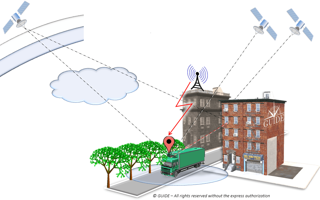
In addition, for terrestrial applications, the satellite signals are affected by several phenomena caused by the immediate surroundings of the receiving antenna. These are the so-called “local” errors, such as terrain, bridges, infrastructures, vegetation and interference of any type. Depending on the areas covered, the trajectories calculated by the terminals deviate more or less from that actually taken by the vehicle (antenna), i.e. the “reference trajectory,” also called “ground truth.”
Figure 1. Sources of error in urban geolocation. (Image: GNSS-GUIDE)
Sources of error in urban geolocation include:
Global errors
Orbits and clocks
Satellite geometries
Ionosphere, troposphere
Local errors
Obstruction, attenuation
Multipath and diffraction
Interference, jamming, spoofing
Terminal errors
Receiving chain
Algorithms and services
Navigation sensors
Classification of position errors
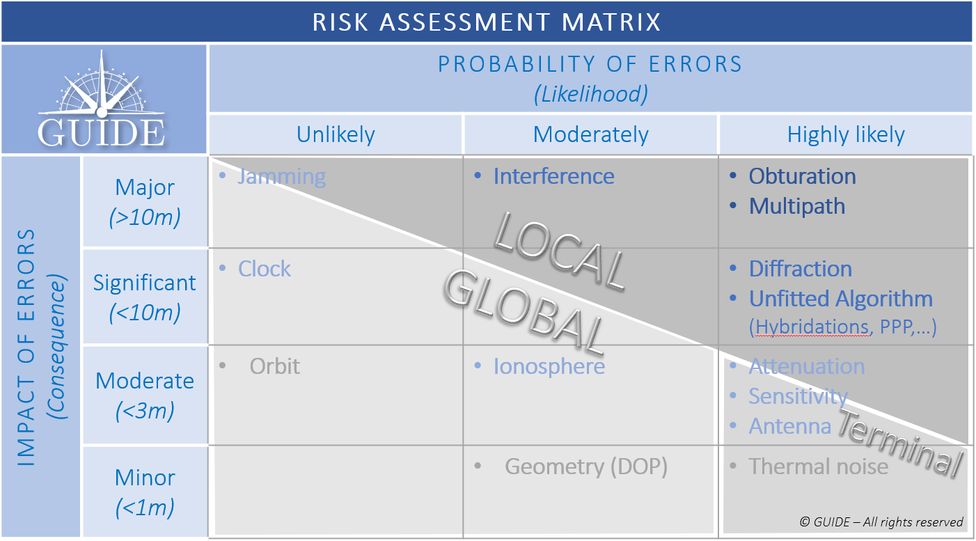
To study those phenomena having the greatest impact and likely to be the most frequent, the different types of errors are displayed as a risk matrix. As the “global” errors can be considered to be handled by the regional SBAS system, the pre-eminence of the so-called “local” errors should be addressed.
Figure 2. GNSS Risk Matrix. (Image: Authors)
Description of the main sources of local errors
To observe the effects of local phenomena on the propagation of signals, a dozen identical receivers — with the same configuration and sharing the same antenna — were mounted on a vehicle and driven through urban and peri-urban areas.
We focus on four particularly impacting phenomena to visualize the trajectories calculated by the receivers.
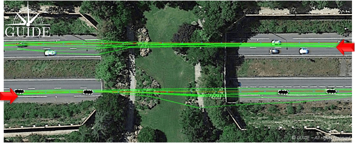
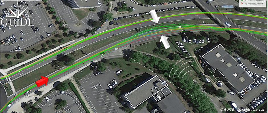
Positioning errors due to bridges
In the picture, below, the test vehicle passes under a bridge in both directions. In both cases, the trajectories diverge under the bridge and converge further on. Here it is easy to understand the shortcomings of results based on a single pass, in other words based on a single measurement.
Figure 3. Effect of alteration of GNSS signals on receivers passing under a bridge. (Image: Auhors)
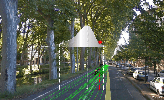
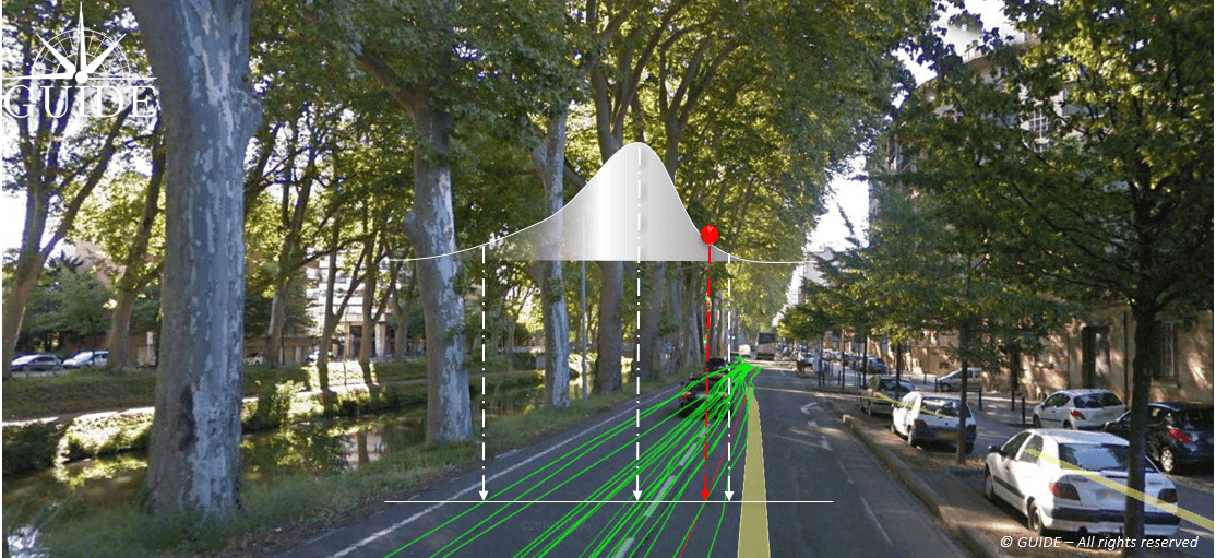
Positioning errors due to vegetation
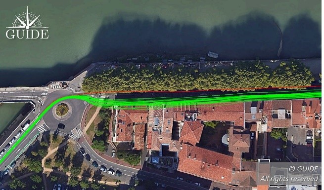
In the image below, the test vehicle is on an avenue lined by trees whose branches and canopy cover the road. The foliage attenuates and, more importantly, diffracts the radio waves arriving from the satellites, thus degrading signal reception. This results in dispersed trajectories. Each receiver provides a different measurement. Note that due to the proximity of buildings, the center of the position distribution, in the presence of multipath, deviates slightly from the reference trajectory.
Figure 4. Effect of diffraction of GNSS signals on receivers passing under tree canopies. (Image: Authors)
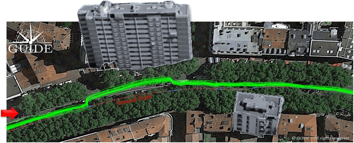
Positioning errors due to buildings
In the composite image (in order to show the main building) below, all the receiver trajectories are deviated towards the building alongside the avenue. The situation highlights the consequences of a phenomenon called “multipath.” When a receiver captures reflected waves, the signal propagation time — used to calculate the pseudoranges — is increased and the accuracy of the end position is degraded. This effect is well known and easily observable during static measurements.
Figure 5. Effects of GNSS signal propagation on receivers near a building. (Image: Authors)
Positioning errors due to interferences
In the image below, the on-board receivers have been disturbed by “transitory” interference. On the outward journey, twenty minutes earlier, no problem had been detected for the trajectories on the other side of the expressway.
On the return journey, this unidentified interference degrades the accuracy of the receivers with a visible dispersion of the trajectories. In other situations, intentional or unintentional interference could completely block out the GNSS band preventing any position measurement.
In this case, the source of the interference seems to come from the bottom right, guided by the two parallel buildings.
Figure 6. Effect of unidentified temporary interference on signals for GNSS receiver. (Image: Authors)
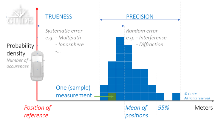
Trueness and precision of position measurements
Receivers of the same batch behave differently depending on the environment. For a predominantly multipath situation, they all converge to the same wrong position. On the other hand, when the propagation phenomena become more complex with multiple diffractions, such as reception under foliage, each receiver produces a position with a different error. For complex environments, we have a combination of these two behaviors.
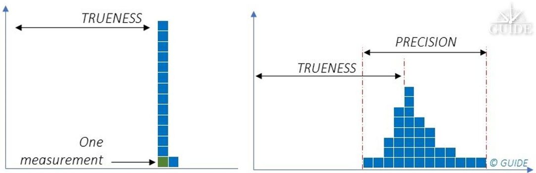
The first behavior is deterministic. Metrology uses the term measurement “trueness,” which stands for “closeness of agreement between the average of an infinite number of replicated measured values and a reference value.”
The second behavior is non-deterministic. In this case, metrology uses the term measurement “precision,” which stands for “closeness of agreement between indications or measured values obtained by replicated measurements on the same or similar objects under specified conditions.”
Terrestrial applications often offer a varied mix of environments where “trueness” and “precision” errors accumulate. It is essential to consider both components in order to characterize and study GNSS receiver performance.
Statistic distribution of the different positioning errors:
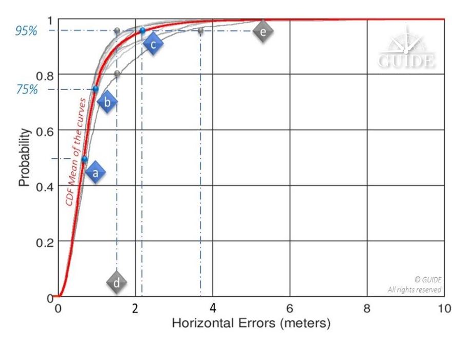
Figure 7. Combination of deterministic and non-deterministic errors. (Image: Authors)Figure 8. A single position measurement at a point has two unknowns: The weight of deterministic (trueness) errors compared to those that are not (precision). (Image: Authors)Figure 9. Statistical distributions of errors for a trajectory (scenario), that is the percentage of all errors (probability) lying beneath a given accuracy level. (Image: Authors)
Above, 95% of the positions calculated during a replay have an accuracy better than 1.5m; this same value is only reached with ~80% of the positions calculated during another replay — see vertical line [d]. The horizontal line [e] illustrates the spread of the horizontal position by considering 95% of the positions of two replays: for one the displayed accuracy is ~ 1.5m and for the other it is degraded to 3.5 m. This curve will always point to the same reference points [a], [b] and [c] recommended by the standard EN16803-1 and corresponds to the percentage of measurements respectively less than 50%, 75% and 95%.
By way of example, the evaluation of a single receiver on board a vehicle travelling in an urban environment does not allow separation of these two components. Indeed, signal degradation determines the degree of dispersion of the “random” component of the measurements. Thus, in certain environments, each additional receiver will produce a different result. However, the analyses of a single onsite campaign relies on just one single sample (single trajectory of the terminal under test), where a panel of measurements is essential. In fact, the available statistics prove insufficient to characterize a receiver, even at the cost of doing long runs.
Figure 10. Visualization of the combined deterministic and non-deterministic errors. (Image: Authors)
Live testing is therefore rather intended for final integration.
On the other hand, a constellation generator will synthesize ideal signals derived from mathematical models, and, in any case, not representative of the real environment. The measurements will then only be deterministic, that is, subject to “systematic” errors. Repeated simulations on the same receiver will always produce the same measurements. Nevertheless, this type of test bench offers many advantages for simulating unobservable situations in the real world.
Disparities in analysis possibilities on position errors based on:
Figure 11. Typical results for repeated measurements obtained, respectively from left to right, with synthetic signals and real-world signals. (Image: Authors)
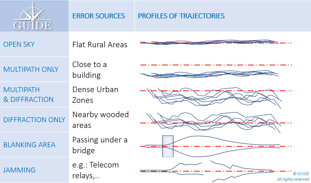
In summary, the main error profiles are described below.
Each situation combines both trueness and precision errors. This latter component requires several runs in the same configuration to determine the potential measurement spread.
Figure 12. Position error profiles (measured trajectories/DUT) depending on the environment. (Image: Authors)
What is GNSS metrology?
As a first approach, characterization of GNSS performance would require many receivers on the same test vehicle. This method is certainly useful in the experimental stage, especially to understand the impact of propagation phenomena on positioning errors. However, it has major disadvantages, both from a logistics point of view and because of the basic metrological requirements.
To obtain reliable and useful measurements, from an operational point of view, the tests must be “representative” of the areas to be covered and “reproducible” to check the results and make valid comparisons, for example, between two receivers, two firmwares, two settings, two antennas and even two hybridizations.
Under these conditions, replay techniques, often referred to as “record and replay,” meet the expected requirements. For the record, this metrology method consists in digitizing the GNSS signals received by the antenna on board the definition vehicle, taking care to collect all the data associated with the tests (VIDEO, INS, DMI, NRTK, …), above all, the ground truth. Thus, at the end of the campaign the GNSS signals and other data are synchronized and restored on a replay bench consisting of an “SDR replayer.”
Replaying the same scenario on a receiver makes it possible to reproduce the recording conditions identically. Each pass generates new measurements, equivalent to using an additional unit, virtually onboard. Compiling the results thus highlights the non-deterministic errors, that is, those which by their random nature emerge from the others.
Test laboratories such as GNSS GUIDE design and market test data that can be replayed directly on the main simulation instruments capable of operating in two modes: simulation and replay. The replay configurations are generally much more affordable than the larger, structurally more complex constellation generators. In addition, the implementation of replay sessions is simple, fast and requires no special training.
In addition to scenarios made on request, the available libraries already cover a multitude of cases, previously inaccessible for an isolated user. They open up the possibility of testing terminals in different latitudes with varied terrain and neighborhoods composed of typical architectures.
Conclusion
The French Space Agency (CNES) has financed several R & D contracts for the development and validation of this replay technique (record and replay). It is already recommended by CEN / CENELEC through the series of EN16803 standards to characterize and classify the performance of GNSS terminals. This methodology complies with the basic principles of metrology.
The test conditions are reproducible and representative of operational conditions. The measurements are repeatable and allow separating the systematic errors (trueness) from the random errors (precision). Measurement uncertainties are also accurately established.
During an on-site measurement campaign, the statistical distributions of two identical receivers on board the same vehicle lead to different results. Thus, no characterization can be established at this stage.
With a replay bench, after several iterations of the same scenario, the average values of the measurements on a CDF tend toward a curve characterizing the performance for that scenario.
Instrumentation dedicated to replay operations is less complex and less expensive. Statistical models of simulations are replaced by scenarios of GNSS signals previously digitized in the field or on constellation generators. Thus, whether they come from a real or synthetic environment, these GNSS signals are easily restored, while drastically reducing the preparation and execution times. The economic benefits of this test technique are now evident and are favoring its adoption by the transportation industries.
References
Niels Joubert, Tyler G.R. Reid, and Fergus Noble (2020), Developments in Modern GNSS and Its Impact on Autonomous Vehicle Architectures
Andrej Tern and Anton Kos (2018), Positioning Performance Assessment of Geodetic, Automotive, and Smartphone GNSS Receivers in Standardized Road Scenarios
Ni Zhu, Juliette Marais, David Betaille, Marion Berbineau (2018), GNSS Position Integrity in Urban Environments
C. Rouch, B. Bonhoure, F.X. Marmet, T. Chapuis, H. Secretan, V. Bienfait, X. Leblan (2016), Measurement campaigns and PVT experiments with new Galileo satellites
B. Calvet, L. Montoya, P. Grandjean, X. Leblan (2015), The GUIDE High-Precision test facility (GNSS laboratory)
G. Duchâteau, X. Leblan, Y. Capelle, W. Vigneau and F. Peyret (2014), Certification of Road User Charging: Approach, standardization and role of laboratories
Tall buildings block GNSS signals, making satellite navigation in urban canyons very challenging. (Photo: RoschetzkyIstockPhoto/iStock/Getty Images Plus/Getty Images)
GPS positioning for navigation and mapping is challenging in urban environments, where GPS signals often are blocked by tall buildings. The following three papers — to be presented at the Institute of Navigation (ION) GNSS+ conference Sept. 19–23, 2022 — explore ways to solve that problem. The full papers will be available at www.ion.org/publications/browse.cfm following the conference.
ALGORITHMS FOR URBAN MAPPING
In this work, the authors use an urban environment model incorporating visibility predictions and remote-sensing techniques, which they tested in a sensor-equipped vehicle in Denver. They use an interacting multiple model (IMM) filter that uses extended Kalman filters to build and verify a map of the signal environment in an urban-canyon setting. The techniques will give ground-vehicle operations the ability to plan for blocked and delayed signals for global path planning.
Zeller, Emma; Strandjord, Kirsten, University of Minnesota; and Wang, Pai, Shanghai Jiao Tong University; “Algorithms for Mapping the Urban Signal Environment for Navigation of Ground Vehicle Operations.”
ADDING VISUAL TO GNSS/INS
GNSS real-time kinematic (GNSS-RTK) positioning is a key technology for surveying and mapping applications. To extend the capability of GNSS in difficult environments, a tight coupling between GNSS-RTK and an inertial navigation system (INS) can greatly improve the results. If the time spent in a GNSS outage is too long or if the kinematic of the survey is too weak, the GNSS/INS solution can be compromised with high navigation errors, ultimately making it impossible to align the heading angle at initialization.
This paper presents an innovative solution to overcome GNSS/INS limitations, minimizing system complexity by using a tightly coupled GNSS/INS solution with a monocular visual inertial SLAM system. This solution is capable of initialization in a few seconds and is very reliable in the long term. This vision/INS/GNSS coupling increases the overall RTK fix rate and broadens the availability of high-precision navigation solutions under challenging conditions.
Bénet, Pierre; Saussay, Brice; Saidani, Mourad; and Guinamard, Alexis; SBG Systems; “Tightly Coupled Inertial Visual GNSS Solution: Application to LIDAR Mapping in Harsh and Denied GNSS Conditions.”
USING 3D BUILDING MODELS
To solve the urban-navigation challenge, the authors propose using a 3D building model to assist GNSS positioning. This type of algorithm is named the 3D building model aided GNSS (3DMA GNSS). It can predict measurement errors and the visibility of the satellites, as line-of-sight or non-line-of-sight. The solution is then derived from the likelihood of the observed and predicted measurements over candidate locations.
The authors propose an innovative method for evaluating the reliability of building models based on the awareness of sky visibility in a specific geographic context. Sky visibility estimation is improved with use of a support vector machine regression and considering low-Earth-orbit (LEO) constellations. The real-time sky visibility could present the update of the surrounding buildings, whereas the predicted sky visibility based on the existing building models remains unchanged. Making use of this inconsistency, the authors could identify areas with the updated building. Additionally, the impacts of the building update monitoring on the 3DMA GNSS are evaluated in an urban canyon.
Xu, Hao-Sheng and Hsu, Li-Ta; Department of Aeronautical and Aviation Engineering, The Hong Kong Polytechnic University; “Urban Buildings Update Monitoring Based on Sky Visibility Estimation using GNSS and LEO.”
How Inertial Systems and GNSS Availability Will Help
Innovation Insights with Richard Langley
ARE WE THERE YET? This was a familiar refrain from the backseats of parents’ cars when traveling to a holiday destination or to grandparents when I was growing up. We didn’t have videos on a display attached to the seats in front of us or (who could imagine?) our own personal communication device on which we could call up games, movies or social media channels.
But I’m not talking about that complaint from our childhoods. I’m asking if we have arrived at the era of the self-driving car. The answer is yes and no. It all depends on what you mean by “self-driving.” We reviewed some of the technologies needed for self-driving or autonomous vehicles in this column in June 2019. And we indicated in the introduction to that column that vehicle autonomy has several levels. SAE International, formerly known as the Society of Automotive Engineers, has defined six levels of autonomy that can be briefly described as Level 0 – no automation; Level 1 – hands on/shared control; Level 2 – hands off; Level 3 – eyes off; Level 4 – mind off; and Level 5 – steering wheel optional.
Already, Level 1 automation is widely available in modern cars with adaptive cruise control, parking assistance, lane-keeping assistance and automatic emergency braking among the features being offered. Level 2 automation, where the automated system takes full control of the vehicle’s acceleration, braking and steering, is available in some production models, although the “hands-off” designation is not to be taken literally — most motor vehicle laws require drivers to keep their hands on the steering wheel. Between Level 2 and Level 3, we have conditional automation — the car can drive itself, but the driver must stay alert and be prepared to take over immediately. Level 3 is high automation, where a computer fully drives the car at certain times on certain routes such as a highway; while the driver can perform other tasks such as reading a book, they must be prepared to take over operation of the vehicle within a few seconds if alerted by the automated system. While test campaigns are still ongoing, some jurisdictions permit Level 3 operation by ordinary drivers on some roads, and customers will soon be able to buy vehicles with this level of automation. Widespread use of Level 4 and Level 5 automation is further off (some would say quite a way off) and remains in development. But famously, last year, Toyota operated Level 4 self-driving shuttle vehicles around the Tokyo 2020 Olympic Village.
A lot more work needs to be done before we will have arrived at the era of the fully self-driving car that will be able to travel on any road, anywhere in the world, all year around, in all weather conditions. In particular, self-driving cars in urban environments (as opposed to highway driving) can be problematic. The required multi-sensor automated systems will include GNSS, but buildings block and reflect GNSS signals, reducing system availability and accuracy. In “Innovation” this month, researchers from the Illinois Institute of Technology report on how inertial navigation systems coupled with wheel-speed sensors and vehicle dynamic constraints can help.
By Kana Nagai, Matthew Spenko, Ron Henderson and Boris Pervan
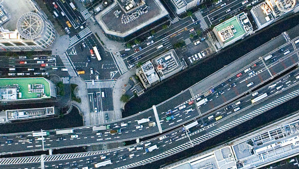
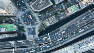
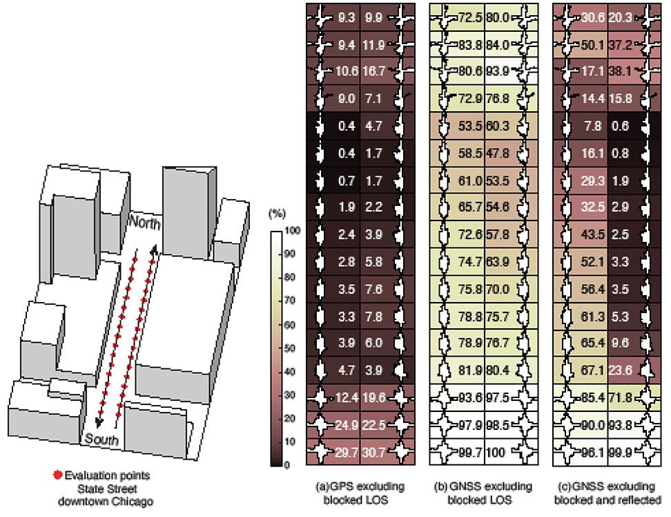
GNSS provides navigation services globally, but satellite visibility in urban areas is limited by high-rise buildings. This creates a mixture of GNSS available and denied environments (see FIGURE 1) — users do not generally know where the system can maintain sufficient levels of accuracy and integrity for a particular application. To begin to address the issue for self-driving cars, we evaluated GNSS-only availability in downtown Chicago.
FIGURE 1 . The figure depicts three types of potential GNSS signal reception: direct LOS signals and blocked LOS signals (left) and reflected LOS signals (right). (Image: Authors)
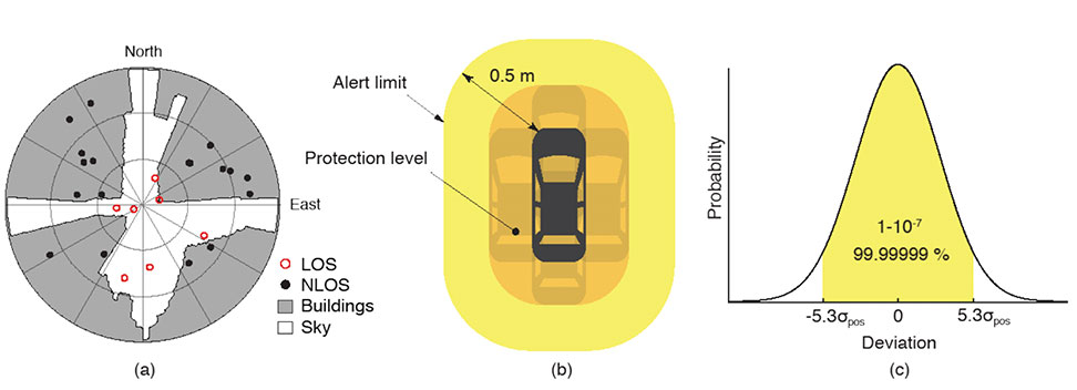
GNSS signal prediction in urban environments has been conducted in previous work. For example, the concept of “shadow matching” was developed to identify GNSS signal blockages in urban canyons. Overlaying sky plots on a hemispherical sky view can be used to distinguish between line-of-sight (LOS) and non-line-of-sight (NLOS) signals (see FIGURE 2a). Reflected rays can be predicted using Householder transformations to reveal potential multipath conditions. Satellites producing blocked or reflected (NLOS) signals should be excluded to maintain integrity.
FIGURE 2. (a) A hemispherical sky view in an urban environment. (b) Illustration of a protection level and an alert limit. To ensure integrity, the protection level must not exceed an alert limit. (c) The allowable probability of exceedance is assumed to be 10−7 in this work. (Image: Authors)
When the number of visible satellites is greater than three, GNSS can resolve vehicle position. However, even in cases where enough satellites are visible, the satellite geometries are generally weak because the dilution of precision (DOP) is adversely affected by the buildings partially blocking the sky. Horizontal positioning error must be bounded by a protection level computed by the vehicle. Then, for navigation to be deemed available, the protection level must not exceed a required alert limit (see FIGURE 2b). The maximum allowed probability of exceedance (see FIGURE 2c) and the alert limit can together be used to determine the maximum allowable position error standard deviation.
Even if the protection level is far below the alert limit in an open-sky environment, it will frequently exceed the alert limit once the vehicle enters a city. GNSS alone is generally not able to maintain availability, so integration with other sensors is needed. Tightly coupling inertial navigation systems (INS) with GNSS using the extended Kalman filter (EKF) provides better estimation in urban environments. The EKF algorithm also enables integration of wheel-speed sensors and vehicle dynamic constraints. These integrated navigation systems will improve availability, but it is still unclear how long such a system can be expected to maintain fault-free integrity in a congested city.
Focusing on the problem of self-driving cars in urban environments, we evaluate protection levels of navigation with practical integrated sensors: GNSS, INS, a wheel-speed sensor (WSS) and vehicle dynamic constraints (VDC). The goal is to develop the means by which we can determine locations where external ranging sources (such as lidar) are needed to maintain continuous navigation with fault-free integrity.
GNSS-ONLY AVAILABILITY
For GNSS availability evaluation, we assume an integrity requirement that the probability of exceeding a 0.5-meter alert limit must be lower than 10−7. The 0.5-meter alert limit therefore corresponds to approximately five times the position standard deviation, so the maximum allowable position error standard deviation is then approximately 0.1 meters. Accuracy at this level clearly requires differential GNSS carrier-phase measurements. We assume a nominal GNSS double difference (DD) carrier ranging error standard deviation of approximately 0.02 meters, and that carrier cycle ambiguities can be readily resolved in an open-sky environment prior to initiation of vehicle motion.
Given the assumptions made of the maximum allowable position error standard deviation and the GNSS ranging error standard deviation, the maximum allowable horizontal dilution of precision (HDOP) is about 5.
FIGURE 3 shows GPS and GNSS availability — the fraction of time the HDOP requirement is met over 24 hours — along a section of State Street in downtown Chicago. The availability results using GPS only and excluding only blocked LOS signals ranged from 0% to 9% along the block and 9% to 30% at the intersections (see FIGURE 3a). Using four full GNSS constellations (GPS, Galileo, GLONASS and BeiDou), availability ranged from 48% to 82% along the block and 72% to 100% at the intersections (see FIGURE 3b).
FIGURE 3. The percentage of GPS or GNSS availability in 3D-mapped downtown Chicago. We exclude satellites producing blocked LOS signals or both blocked and reflected LOS (NLOS) signals from the measurements. Each column expresses a lane of southbound or northbound travel. The availability is the percentage of total time when HDOP meets the self-driving car integrity requirements in 24 hours. (Image: Authors)
When we also excluded satellites producing reflected LOS signals that reach the vehicle, the availability dropped significantly at every point (see FIGURE 3c). We assert that FIGURE 3c expresses the reality of GNSS availability because building-reflected multipath signals degrade positioning accuracy and would affect integrity negatively. It’s obvious from these results that GNSS alone is insufficient to meet the autonomous driving requirements in an urban environment, and multi-sensor integrated navigation systems are needed to augment poor GNSS signal availability.
MULTI-SENSOR INTEGRATION
We begin by considering tightly coupled INS/GNSS integration using an EKF, and then integrate a realistic sensor suite including WSS and vehicle dynamic constraints that enforce resistance to lateral sliding and vertical movement. If it is known from another source that the vehicle is not moving (for example, it is in the parking gear), a static mode constraint (SMC) can also be applied.
INS/GNSS Integration. Tightly coupled INS/GNSS integration with an EKF uses the INS measurement to predict vehicle motion. The continuous process model uses a state vector having the position in the navigation frame, the velocity, the attitude, bias errors and cycle ambiguities, with the input vector having accelerometer-specific force measurement in the body frame and gyro-rotation-rate measurements. A white-noise vector drives the inertial measurement unit (IMU) states.
The GPS/GNSS measurement model includes the measurement vector having carrier and code phases, and the observation matrix containing LOS vectors and the vector of white receiver thermal noise.
INS/GNSS/WSS/VDC Integration. For the vehicle in motion, we developed a model consisting of a WSS measurement in the along-track direction, a non-holonomic constraint resisting lateral sliding, and a holonomic constraint on vertical movement (see FIGURE 4).
The INS/GNSS/WSS/VDC integration using the EKF consists of the process model and the measurement models.
INS/GNSS/SMC Integration. The static mode constraint provides zero-velocity measurements to the EKF measurement update to mitigate position error propagation. We use SMC only when it is known that the vehicle is not moving; for example, when the vehicle is in the parking gear.
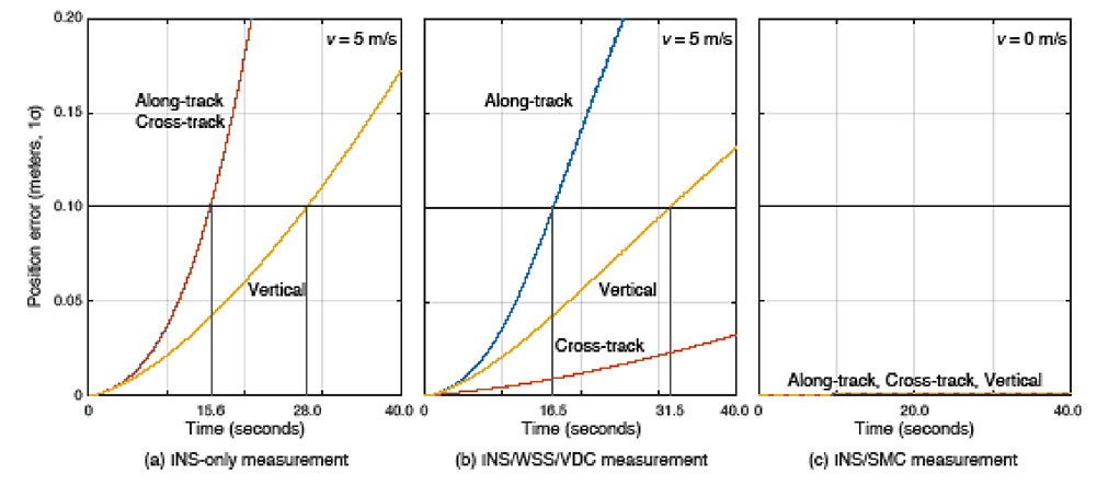
Error Propagation Analysis. We tested the time from perfect initialization to when position error exceeds 0.1 meters in GNSS-denied environments. FIGURE 5 shows the error growth in the along-track (x), the cross-track (y) and the vertical (z). The error specifications for a STIM300 tactical-grade IMU are used in this analysis. The standard deviation of the WSS measurement noise is assumed to be 0.05 meters per second, and the standard deviation of the movement constraint violations is 0.001 meters per second. The vehicle is moving at 5 meters per second except when we test the SMC.
FIGURE 5. The vehicle position error growth vs. time in the along-track (x), cross-track (y) and vertical (z) directions. Each graph represents the navigation system introduced in the multi-sensor integration section. The vehicle is moving at 5 meters per second (a and b) or 0 meters per second (c). (Image: Authors)
The INS can coast 15.6 seconds before the position error standard deviation exceeds 0.1 meters in both the along-track and the cross-track directions (see FIGURE 5a). The INS/WSS/VDC can coast 16.5 seconds in the along-track direction, and significantly more than 40 seconds (the simulation duration) in the cross-track direction (see FIGURE 5b). In static mode, INS/SMC estimate errors do not grow with time in any direction, as expected (see FIGURE 5c). In GNSS-denied environments, the non-holonomic constraint suppresses the cross-track position error, but the WSS measurement hardly affects the along-track position error. The SMC works perfectly, but the usage is limited to when the vehicle is known to be stationary.
SIMULATION SCENARIO
We imagine a future driverless-car mission scenario in which multi-sensor navigation systems are practicable. To minimize congestion in a city, autonomous vehicles will be held outside the urban core when not in use. In the clear open-sky environment, a vehicle in a parking lot completes GNSS initialization using the INS/GNSS/SMC system. Once requested for action, the vehicle departs for the city from the parking lot, and the motion of the vehicle improves alignment by the INS/GNSS system. Safe navigation can be ensured using the system to provide continuity under overpasses and bridges in the open-sky environment. Upon entering the urban core, navigation becomes more dependent on the INS/WSS/VDC system.
A reasonable numerical target for differential GNSS initialized position error is 0.02 meters, and for the INS alignment yaw angle error 0.1 degrees.
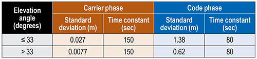
Local GNSS multipath errors from nearby vehicles will vary with the satellite elevation angle. Prior experimental results show that lower elevation-angle satellite signals (below 33 degrees) are much more likely to be impacted by multipath than higher ones (see TABLE 1).
TABLE 1. The nominal GNSS multipath error values in the simulation.
INITIALIZATION AND ALIGNMENT
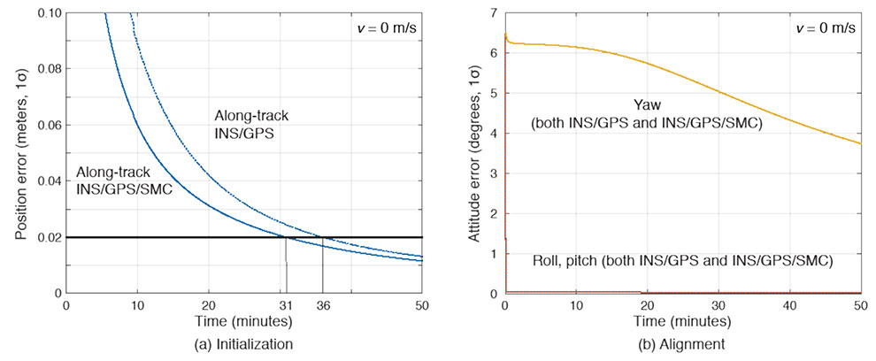
Initialization takes place in a parking lot with a clear sky view. A vehicle is in the parking gear, enabling SMC to be applied. FIGURE 6a shows a typical example: with INS/GPS/SMC, system initialization takes about 31 minutes, and with INS/GPS, about 36 minutes. Therefore, SMC does speed up GPS initialization, although the improvement is modest.
The yaw angle is not aligned during the initialization, but roll and pitch are immediately aligned (see FIGURE 6b). Earth’s gravity affects roll and pitch angle alignment but not yaw angle.
FIGURE 6. (a) Comparisons of initialization time between INS/GPS and INS/GPS/SMC in an open-sky environment. The INS/GPS/SMC system initializes rapidly. (b) Transitions of roll, pitch, yaw alignment during the initialization. Yaw angle alignment cannot be performed when the vehicle is stationary. (Image: Authors)
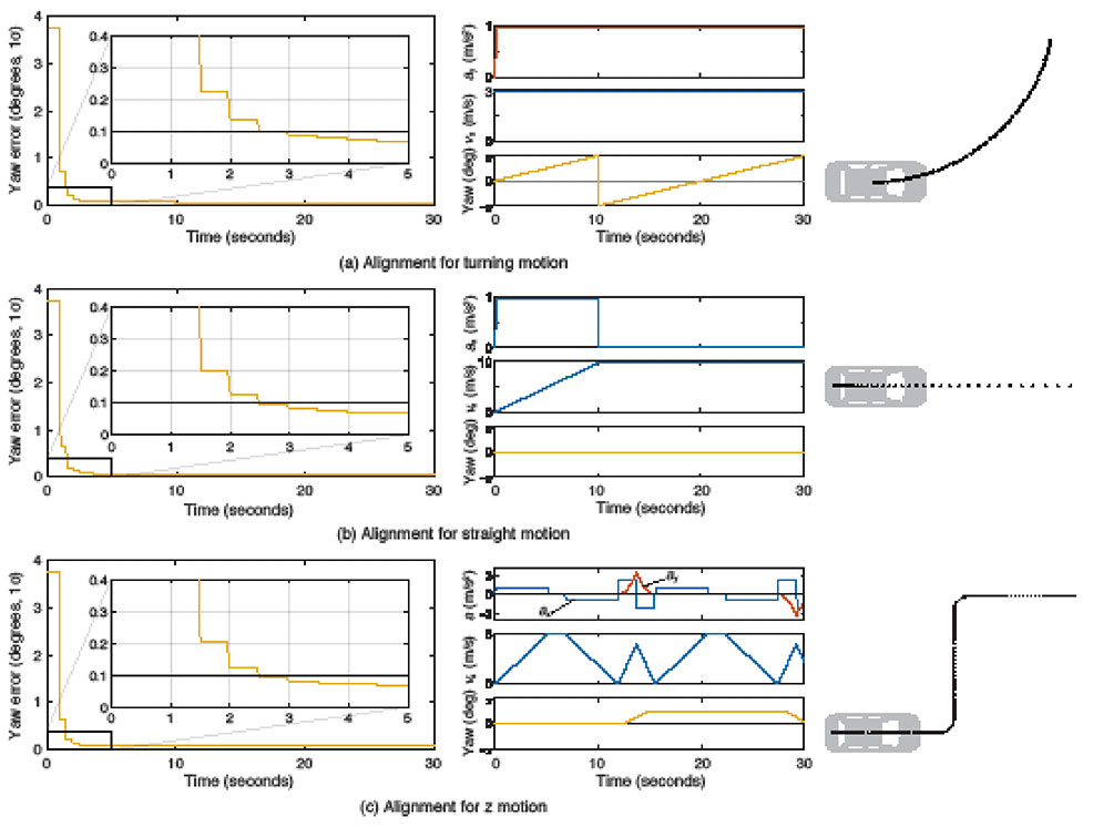
Yaw angle alignment cannot be performed when the vehicle is stationary or moving with constant velocity. Accelerated motion, either straight or turning, is required. FIGURE 7 shows the behavior of the yaw angle error standard deviation using the INS/GPS system when centripetal (see FIGURE 7a) or tangential (see FIGURE 7b) acceleration is applied. The yaw angle can be aligned in a couple of seconds for either type of acceleration. To represent typical initial motions of self-driving cars, we model a parking-lot departure via a “Z”-shaped path. In this scenario, the yaw alignment error reaches 0.1 degrees within a couple of seconds (see FIGURE 7c).
FIGURE 7. The behavior of yaw angle error when centripetal (a) or tangential (b) acceleration is applied; (c) shows the behavior while following a z-shaped path. The yaw angle can be aligned in a couple of seconds in each case. (Image: Author)
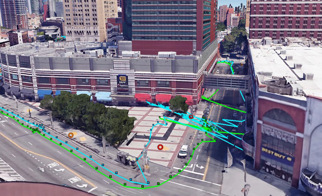
EVALUATION IN URBAN ENVIRONMENTS
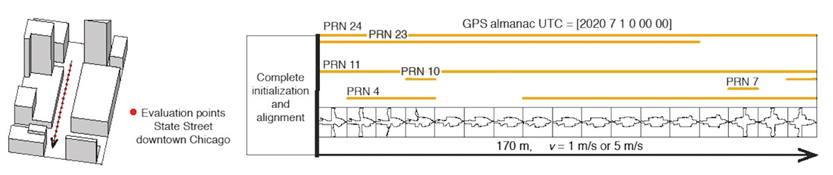
After initialization and alignment in the open-sky environment, we simulated the vehicle traveling into the urban core. The urban environment in our study is 3D-mapped State Street in Chicago, which runs north-south and transits from low-rise neighborhoods to central downtown. We selected one congested section surrounded by tall buildings and computed the position error standard deviation along the path. The evaluation points are at 10-meter intervals over a total distance of 170 meters. The yellow lines in FIGURE 8 denote the visible satellites, identified by their pseudorandom noise (PRN) code numbers, at each point. We assume for convenience that the INS/GPS system is initialized and aligned at the first evaluation point. In reality, we would expect a degraded initial condition because we are starting the simulation in an urban canyon.
FIGURE 8. Evaluation points and PRN numbers of visible satellites at each point. (Image: Author)
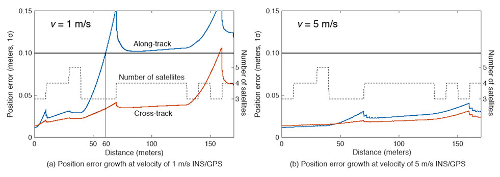
In the first simulation, the car equipped with the INS/GPS system moved either 1 or 5 meters per second. The y-axis in FIGURE 9 represents the position error standard deviation, and the x-axis represents the distance in meters. The dotted line expresses the number of visible satellites. The error when the vehicle velocity is 1 meter per second exceeded the maximum allowable position error standard deviation of 0.1 meter, at the distance of 60 meters. However, when the velocity was 5 meters per second, the maximum allowable position error standard deviation was never reached. It is also clear from the figures that error propagation is significantly affected by the number of visible satellites.
FIGURE 9. A comparison of position error growth between velocities of 1 meter per second and 5 meters per second. (Image: Author)
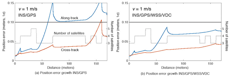
In the second simulation, we compared two different navigation systems, INS/GPS and INS/GPS/WSS/VDC. The vehicle moved at 1 meter per second in the same urban environment. The INS/GPS/WSS/VDC system does provide relief, but the error propagation is still clearly affected by the number of visible satellites (see FIGURE 10).
FIGURE 10. A comparison of position error growth between the INS/GPS and INS/GPS/WSS/VDC systems for a velocity of 1 meter per second. (Image: Authors)
In GNSS-challenged environments, INS error propagation is a function of time. When a vehicle moves faster, it clears the blockage area more quickly, reducing the impact of INS drift — a function of time, not distance. In contrast, GNSS error is completely determined by location. Because INS error propagation depends on how long the vehicle stays in an area of GNSS outage, protection levels for trips through the same area will be different if the vehicle is smoothly cruising or gets stuck in a traffic jam.
CONCLUSION
To gain a better understanding of how long and under what local conditions multi-sensor integrated navigation systems can maintain fault-free integrity, we evaluated navigation positioning errors in 3D-mapped downtown Chicago. The system we developed consists of sensors with which self-driving cars would reasonably be equipped: GNSS, INS, WSS and dynamic constraints. We showed that INS/GPS position errors along the path depend very strongly on the vehicle’s speed. When the system is augmented with WSS/VDC, position errors are suppressed, but the error propagation is still strongly influenced by the number of visible satellites.
ACKNOWLEDGMENTS
The research described in this article is supported by the National Science Foundation. Figure 1 was created by Alexis Arias of the Landscape Architecture + Urbanism Program at the Illinois Institute of Technology (IIT). The authors greatly appreciate the advice and help of Nilay Mistry from that program.
This article is based on the paper “Evaluating INS/GNSS Availability for Self-Driving Cars in Urban Environments” presented at ION ITM 2021, the virtual 2021 International Technical Meeting of The Institute of Navigation, Jan. 25–28, 2021.
KANA NAGAI is a Ph.D. candidate and research assistant in mechanical and aerospace engineering at IIT.
MATTHEW SPENKO is a professor of mechanical and aerospace engineering at IIT. He earned his M.S. and Ph.D. degrees in mechanical engineering from the Massachusetts Institute of Technology.
RON HENDERSON is a professor and director of the Landscape Architecture + Urbanism Program at IIT. He earned his Master of Landscape Architecture and Master of Architecture from the University of Pennsylvania.
BORIS PERVAN is a professor of mechanical and aerospace engineering at IIT. He earned his M.S. from the California Institute of Technology and Ph.D. from Stanford University.
A new map method opens up parking continuous-environment mapping for enhanced low-cost urban navigation. Collectively recorded context data by many identical platforms gather similar sensor readings when operating in a given area. Further processing integrates the data with a map and feeds the summarized results to a user.
ByIvan Smolyakov, Evgeny Klochikhin and Richard B. Langley
Complex, dynamic urban environments comprise millions of devices with localization capabilities. While GNSS remains a primary positioning tool, its performance is subject to significant degradation from blocked signals, multipath and non-line-of-sight (NLOS) signal reception. In aided navigation, a positioning filter with GNSS measurements integrates data from various sensors and correction streams to compensate for these disadvantages.
Low-cost platforms are limited with the variety and quality of sensors on board, as well as by processor performance and battery capacity. Positioning routines must be computationally light, energy efficient and make the most productive use of available data.
One new research area covers use of crowd-sourced GNSS data. Many vehicles now include some type of native wireless connection capability, which could be complemented by a designated third-party device.
The growth in connectivity brings an opportunity to access a stream of sensor data produced by a high number of devices operating in a localized urban area. Here, we explore the idea of creating a GNSS signal-strength map using the connected vehicle GNSS data stream and then use the map as statistical information for Kalman filter parameters tuning. This approach improves filter reaction to the environment and produces a positioning accuracy improvement.
SYSTEM ARCHITECTURE
C/N0 levels of reflected and diffracted signals are more likely to be lower than that of the LOS signals. We propose that the C/N0 level averaged during a given period among all satellites tracked in a given area would correlate with a higher probability of multipath-contaminated and NLOS signal reception.
A sufficient number of C/N0 readings associated with a given space-time cube should be collected to compute the statistics populating the signal-strength map. However, the city environment does not remain static: new construction occurs, traffic congestion shifts, and so on. Therefore, the C/N0 space-time statistics must be continuously updated in real time to reflect these changes. Additionally, the solution must be highly scalable as the market of connected vehicles is growing and so is the volume of the streamed data.
A recent advance in cloud-based data-stream processing, a data flow model treats an input data stream as something that will never become complete. A derivative of that model is Flink, an open-source framework capable of both unbounded data (stream) and bounded data (batch) processing, while treating bounded data as a special case of the streaming applications.
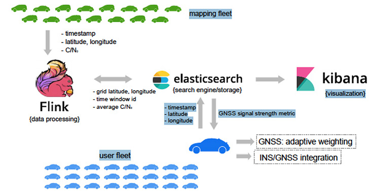
We use Flink as a core library for the environment mapping architecture as it fits the needs of event-time processing while being a highly scalable solution. The processing enables calculating necessary statistics based on a moment of time a reading occurred rather than based on a moment of time the reading arrived at the cluster. The proposed system architecture is presented in Figure 1.
The connected vehicle mapping fleet transmits packets of the GNSS receiver readings via cellular Internet connection to the server at 1 Hz. Each packet contains a timestamp in the UTC time system, the geographic coordinates determined by the proprietary positioning algorithms of a connected vehicle, and the C/N0 measurements per each tracked satellite.
The geospatial processing block calculates the average C/N0 metric among the readings of a given space-time cube. Computed statistics are sent to Elasticsearch, updating the map in real-time. Elasticsearch is an open-source, distributed search and analytics engine integrated with Kibana, an open-source data visualization tool. User platforms request the average C/N0 metric from the search engine with their UTC timestamp and coordinates and apply it in the processing filter.
PILOT PROJECT
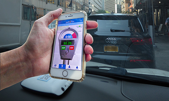
The system is currently in prototype. Collection of the data populating the map was performed with two positioning boards designed by Parkofon Inc. and installed on the dashboard of a vehicle (Figure 2).
Figure 2. Mapping setup: Parkofon board is installed on the dashboard of a vehicle. (Image: Authors)
Lack of a high number of vehicles for the data collection campaign was compensated with an extensive piloting time (17 hours, 43 minutes) in a limited area, driving the same roads repeatedly. Two areas of New York City were the subject of extensive mapping.
Tests concentrated on two sectors with different GNSS signal strengths: sector A, a relatively open-sky area; and sector B exhibiting deep urban canyon conditions. The mapped average C/N0 is denoted as .
The of the less obstructed sector A = 39.3 dB-Hz, while that of the more obstructed sector B is lower: 18.1 dB-Hz. This tendency is repeatable throughout the surveyed area and allows for further GNSS signal-strength map integration into the algorithms at the user side.
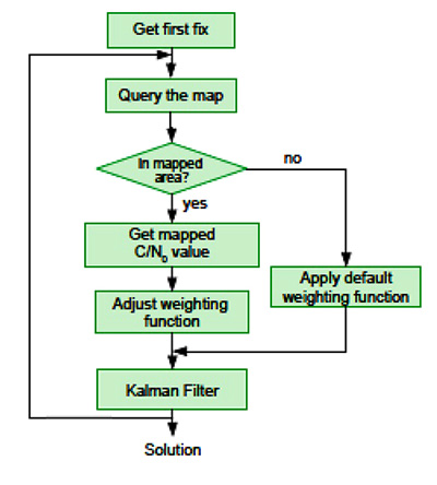
It is a challenge to find an optimal set of urban navigation filter parameters, as the signal obstruction environment changes significantly with the moving positioning platform. Our approach adjusts parameters of the GNSS observation weighting function with respect to the retrieved from the map. The algorithm scheme appears in Figure 3.
When the first position fix is obtained, the algorithm sends a request to the server with the timestamp and the coordinates determined at the previous epoch. If one is available in the current user area, the server response includes the metric retrieved from the GNSS signal-strength map. Next, the GNSS observation weighting function is adjusted according to equations given in the full technical paper (see Acknowledgment section).
PRACTICAL RESULTS
Algorithm performance was evaluated by analysis of the distances between the coordinates calculated with our engine and the centerline of the road in two downtown and two residential areas. For an estimated 86 percent of the track, our proposed map-aided weighting performed better than when the default weighting function was applied during the whole track.
The map-aided weighting of the observations brings approximately 25 percent and 35 percent accuracy improvement in the dense urban area and in the intermediate residential environment respectively. Additionally, there were instances of faster solution re-convergence when fix was lost due to insufficient number of the satellites tracked in narrow streets or under obstructions (see Figure 4).
Figure 4. Example of faster map-aided solution re-convergence. (Image: Authors)
FUTURE WORK
For the mapped average C/N0 levels to be unbiased, normalization procedures must be implemented. This would soften or eliminate hardware constraints on the mapping fleet and facilitate its growth. With more data available, the temporal discretization of the map needs to be implemented as satellite geometry and multipath environment change throughout the day.
Optimal dimensions of the mapped space-time cube remain an open question: more real-world data needs to be collected to provide better mathematically-derived estimations. We plan to investigate the benefits of a variable-dimension space-time cube with respect to the area and the mapping fleet density. We also plan to extend the environment map-aided filter tuning to a multi-constellation GNSS approach integrated with inertial navigation systems and other sensors.
The technique is commercially implemented in Parkofon, a fully automated parking payment and guidance system that helps people find cheaper, safer and easier parking. The platform includes a mobile app and device placed in the car to guide drivers to open parking spaces in real time and charge them only for actual time parked in designated garages. Parkofon also offers real-time on-street space availability.
Acknowledgments
This article draws on a paper presented at ION GNSS+ 2018. For the full paper, see www.ion.org/publications/browse.cfm. Research is supported by the Natural Sciences and Engineering Research Council of Canada.
MANUFACTURERS
Experimental datasets were collected with a Septentrio AsteRx-m2 receiver and Maxtena M1227HCT-A2-SMA antenna. Parkofon boards carry a u-blox M8N receiver module and a Taoglas CGGBP.25.4.A.02 patch antenna.
IVAN SMOLYAKOV is a Ph.D. student in the Department of Geodesy and Geomatics Engineering at the University of New Brunswick (UNB).
EVGENY KLOCHIKHIN is CEO of Parkofon Inc., a smart mobility company utilizing the Internet of Things to guide drivers to open parking. He holds a Ph.D. in Public Policy and Management from the Manchester Business School, UK.
RICHARD B. LANGLEY is a professor in the Department of Geodesy and Geomatics Engineering at UNB.
By Tommaso Panicciari, Mohamed Ali Soliman and Grégory Moura
All images provided by the authors
A real-time system combining a simulator and a GNSS propagation model reproduces an authentic multipath environment. The propagation model relies on a 3D-model reconstruction of the urban environment, which generates a multipath signature strictly dependent on the location of the receiver’s antenna. This yields important results for a moving vehicle, which may be affected by very different multipath conditions depending on trajectory and location.
Positioning and navigation can be degraded in urban environments by multipath, and the error can increase considerably if not properly compensated. In situations where the line-of-sight (LOS) is obscured by surrounded buildings, the receiver may still be able to navigate by using the non-line-of-sight (NLOS) signal, which originates from single or multiple reflections/diffractions of the GNSS signal.
The use of 3D models has been one of the preferred solutions to recreate the multipath environment as seen by a GNSS device. This solution brings the capability to generate a multipath signature that is representative of the position of the antenna in a specific time and space. However, this solution comes with a certain degree of complexity. In fact, an accurate 3D model is required to simulate the obscuration of the GNSS signal, and a good propagation model is needed to generate phenomena like reflection and diffraction.
Figure 1. Example of propagated signal simulation. (Image: Tommaso Panicciari, Mohamed Ali Soliman and Grégory Moura))\
3D models have become more accurate and widely available and are mainly used to predict the satellite availability in specific locations, for example in evaluating the signal availability in urban canyon, and for both reflection and diffraction. Other uses of 3D models are as an aiding tool to assist navigation, sometimes together with an INS solution.
In this article, we present a novel real-time system capable of simulating realistic multipath in different environments. The system can simulate multiple GNSS constellations and is comprised of a GNSS simulator interfaced to a propagation model. The system can create a whole range of signals, effects, error models and trajectories in a real-time closed loop. The propagation model controls the simulation of multipath from the interaction of the GNSS signal with the 3D scene and objects. This article describes a novel real-time system for the simulation of realistic multipath in different environments and compares simulated and field-test data. The comparison is based on signal availability, horizontal error, carrier-to-noise (C/N0), pseudorange and Doppler residuals.
RAY-TRACING WITH 3D MODELING
The model simulates the propagation of GNSS signals in constrained environments, considering obscurations and multipath. It uses a proprietary ray-tracing kernel (based on bounding volume hierarchy techniques using processing unit [GPU] resources) coupled with geometrical optics and uniform theory of diffraction to compute the interaction between the signal and the local environment. The computation uses as main input a synthetic environment (that is, geometrical and physical modeling of a real or realistic environment) to assess the impact of obscurations related to signal availability issues and multipath (the cause of fading effects and performance problems).
The objective of ray-tracing is to find all the possible paths from the observer to the source of the signal considering a limited number of interactions per emitted rays. A ray-tracer (or ray-tracing algorithm) uses a primary grid to cast primary rays. Then, it iteratively computes the possible interactions between these rays and the virtual scene (often defined using triangles). If those interactions exist (if they comply with the law of physics) and if the number of interactions to reach the emitter is below the maximum number of interactions set by the user, then a ray (or multipath) is created. This is a deterministic method that can be used to calculate the obscuration due to the local environment (and therefore detect the signal availability) and the geometrical characteristic of the computed path. Combined with physics modeling, path attributes such as received power, delay, Doppler, and phase are also provided.
The main characteristics of ray-tracing techniques to model GNSS propagation are:
All the signals arriving at the receiver can be model-based on the virtual environment.
As it is a deterministic method, the more realistic the environment modeling, the more compliant with reality the results. Moreover, the simulation results are repeatable.
The specular multipath can be displayed in 3D, and the attributes (for example, receiver power, phase, polarization, Doppler, geometry of the ray) are known. For example, this is relevant when the effect and signature of the environment on the propagation signal need to be studied and understood.
Nonetheless, ray-tracing techniques must account for three major difficulties:
They are time-consuming algorithms. Indeed, depending on the complexity of the scene (defined in terms of the number of triangles), a combinatorial problem to find the possible multipaths reaching the receiver makes the ray-tracer very resource-demanding. That is the reason why the most difficult task to achieve during the coding of a real-time ray-tracing algorithm is to develop acceleration techniques to quicken the computation process. Several solutions exist to either improve the intersection determination (for instance, based on spatial hierarchies such as bounding volume hierarchy [BVH] techniques), or to decrease the number of cast rays (often based on adaptive sampling techniques), or even to replace rays with beams or cones. Moreover, it is possible today to use the resources of graphic boards to accelerate the computation. Indeed, as ray-tracing can be coded by a large number of primary functions that can be treated simultaneously, it can be easily ported into GPU.
Their accuracy depends on the resolution of the primary grid. Details and therefore rays may be missed if the 3D scene is made of small details. This issue is called aliasing. Aliasing artefacts are raised for instance in parts of the scene with abrupt changes (such as edges) or in complex areas with lots of constituent objects. Solutions (or antialiasing techniques) exist to overcome this issue such as adaptive or stochastic samplings.
When it is combined with geometrical optics, these algorithms only compute the specular rays. Even if some techniques exist to model the scattering signals, only physical optics can render the global signal with high fidelity.
MULTIPATH SIMULATION SYSTEM
The proposed system can model two of the main propagation issues encountered in urban environments, such as obscuration (which leads to limitations in signal availability) and multipath (which generates interference that causes fading of the signal and positioning errors). To model realistically such a complex phenomenon, the system uses a GPU ray-tracing algorithm combined with geometrical optics and uniform theory of diffractions. The ray-tracing algorithm relies on 3D-model reconstructions of the urban environment. The computed obscuration and multipath effects are then used to generate signal corrections (in terms of power, delay and Doppler variation) to be used in the GNSS simulator, which generates the carrier, code and navigation messages for different GNSS constellations into a single RF output. Some of the advantages of this system is its ability to run in real time, and to visually show all the reflections/diffractions of the GNSS signals that cause multipath interference.
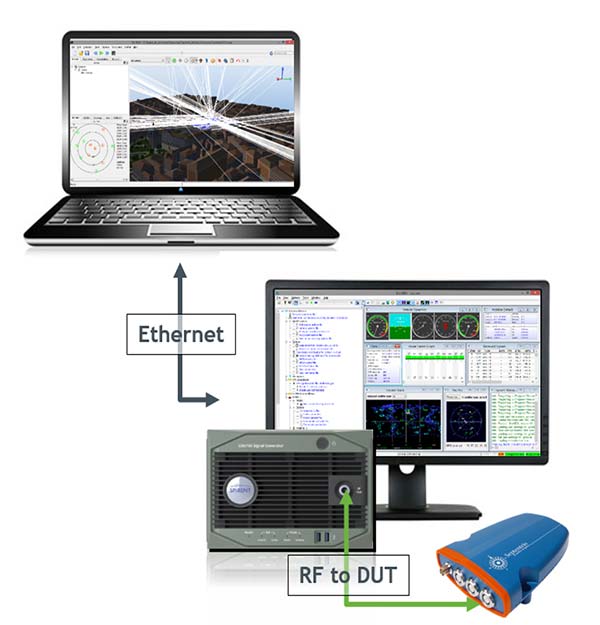
Figure 2 shows the diagram of the system set up in conductive mode. The system includes a SE-NAV PC controller, simulator software suite controller, GNSS simulator and device under test (DUT). A different mode is also available called over the air (OTA). This mode uses an anechoic chamber and a set of antennas distributed uniformly to generate the RF signal including the multipath. The DUT can then be placed at the center of the chamber and will be able to receive LOS and NLOS signals from different angles of arrival.
Figure 2. System diagram that shows propagation simulator controller (top), the GNSS simulator (bottom) and the device under test connected to the RF output of the simulator. (Image: Tommaso Panicciari, Mohamed Ali Soliman and Grégory Moura)
The GNSS simulator software suite is used to generate and control the generation of the satellite signals (including multipath) at RF, whilst the propagation simulator is used to calculate the propagation information (delay, Doppler and attenuation) of the reflected signals through a 3D urban model. The propagation software is interfaced with GNSS simulator software by means of a package of remote-control facilities that greatly enhances the flexibility of the propagation simulator. Those commands can be sent and received through the transmission control protocol/use datagram protocol (TCP/UDP) with different data streaming rates (10 Hz was used for this article).
It is also important to point out that the propagation simulator computes all the possible multipath signal generated by the 3D model given the position of the satellites and receiver. However, the physical limitation of the number of channels in the simulator causes the rejection of some rays. This rejection or filtering process can be done according to power (used in this article) or delay.
EXPERIMENT SET-UP
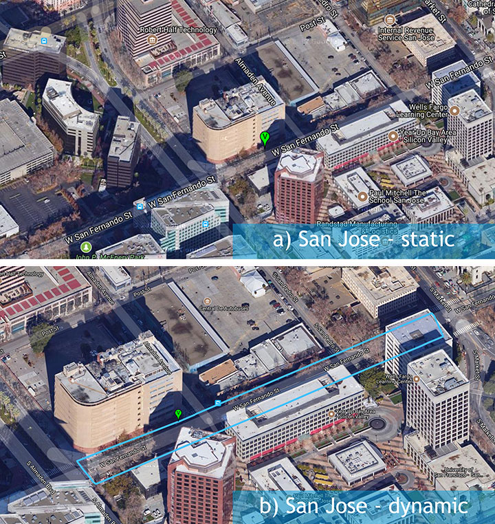
A set of different field-test campaigns where carried out in August 2016. Each campaign aimed to evaluate the ability of the system to assess the performances of a GNSS receiver using simulated signals in urban environments. Figure 3 shows the trajectory (blue line) used for the experiment in an urban environment — San Jose, California — with a static (a) and dynamic (b) scenario.
Figure 3. A set of three measurement campaigns where carried out during Aug. 9–10, 2016: a) urban environment with static antenna; b) urban environment with dynamic antenna. (Image: Tommaso Panicciari, Mohamed Ali Soliman and Grégory Moura)
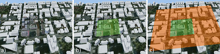
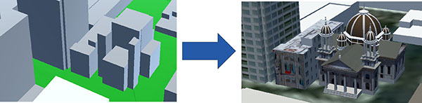
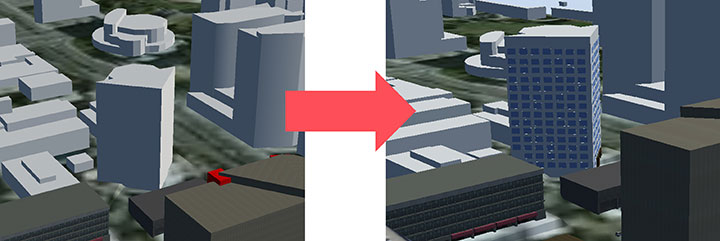
Figure 4 shows the 3D scene used to replicate the San Jose urban environment. The buildings in close proximity of the antenna (green area in Figure 4b) contain details like material, 3D facade and windows. In contrast, the buildings far from the antenna were only corrected for height, and the material was modeled as concrete only.
Figure 4. The San Jose model contained most of the details around the receiver antenna (b), with only height corrected for buildings far from the antenna (c). (Image: Tommaso Panicciari, Mohamed Ali Soliman and Grégory Moura)
An exception was made for one building in San Jose because its complex architecture was believed to contribute to more reflected rays than would a more simplistic box (concrete) model (Figure 5).
Figure 5. Improvement (right) in one San Jose building because its complex architecture was believed to generate more reflections than the more simplistic box model (left). (Image: Tommaso Panicciari, Mohamed Ali Soliman and Grégory Moura)
EXPERIMENT RESULTS
A direct comparison of C/N0 power, pseudorange residual, and Doppler residual was performed between the field test and simulation.
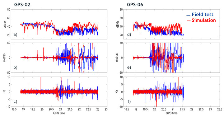
San Jose Static Results. Figure 6 shows the results obtained from the San Jose static scenario for satellites PRN02 and PRN06: C/N0 ratio, pseudorange residual and Doppler residual for field test (blue line) and simulation (red line). Although the simulation sometimes creates deeper fading than in the field test, a first comparison indicates a good correlation of simulated data with field-test data.
Figure 6. Carrier-to-noise ratio (top), pseudorange residual (middle) and Doppler residual (bottom) for PRN 02 (left column) and PRN 06 (right column). (Image: Tommaso Panicciari, Mohamed Ali Soliman and Grégory Moura)
The signature of the multipath caused by this urban environment is visibly captured in the simulation. More interestingly, the pseudorange residuals and, to a lesser extent, Doppler residuals also indicate that the model is replicating the dynamics of the multipath environment in close correlation with the field test.
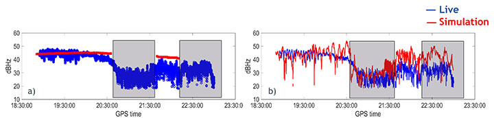
Figure 7 shows the C/N0 obtained from the field data (blue), and simulated data (red) with only obscuration (a) and with obscuration and multipath (b) for the static scenario.
It can be noticed that the receiver can still track PRN02 without the LOS, therefore, relying on just the NLOS signal. This can be clearly seen in Figure 7a where a sudden drop in power is associated to an obscuration of the same satellite (based on our 3D urban model).
Figure 7b shows the C/N0 obtained from the simulation (red line) when both obscuration and multipath were enabled. In this case the receiver could track the satellite even in the case of only NLOS as in the field test.
Figure 7. Carrier-to-noise ratio for satellite PRN02 with only obscuration (a) and with multipath (b). (Image: Tommaso Panicciari, Mohamed Ali Soliman and Grégory Moura)
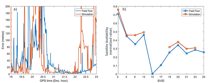
The positioning error for the San Jose static scenario is shown in Figure 8a. The simulation and field-test data have a comparable error. The error is relatively big at the beginning of the simulation and decreases after time 20.6. At the time 22.3, a moderate increase in the positioning error is visible in the field data until the end of the test. The simulation also shows a similar trend in this last part of the test, but tends to generate a higher positioning error.
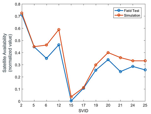
The satellite availability is shown in Figure 8b for both simulated (red) and field test (blue). The availability of the satellites generated with simulated data is in close relationship with the field data. However, some satellites could not be tracked in the simulation.
Figure 8. a) positioning error for field-test (blue) and simulation (red); b) satellite availability for field data (blue) and simulation (red). (Image: Tommaso Panicciari, Mohamed Ali Soliman and Grégory Moura)
The importance of the accuracy of the 3D scene is evident in this example. In fact, we noticed that one of the buildings that was simulated as a simple concrete box was more complex in the real environment. Therefore, we applied some modifications to scene, as in Figure 9.
Figure 9. 3D scene improvement. (Image: Tommaso Panicciari, Mohamed Ali Soliman and Grégory Moura)
After those changes, a general improvement in the results was visible, but most importantly, the missing satellites could finally be tracked by the receiver (Figure 10).
Figure 10. Satellite availability for field data (blue) and simulation after scene improvement. (Image: Tommaso Panicciari, Mohamed Ali Soliman and Grégory Moura)
SAN JOSE DYNAMIC TEST RESULTS
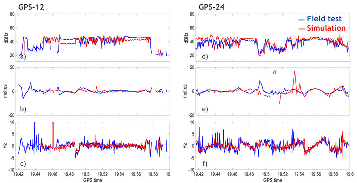
Similar results were obtained with the dynamic test in San Jose. Figure 11 shows the results obtained for satellites PRN12 and PRN24. The walking trajectory included two points where the antenna was stopped because of a traffic light. Those points correspond to a relatively flat C/N0 that can be clearly seen in the field test and simulation data for both PRNs. When, instead, the antenna was moving, a higher variation in the C/N0 is noticeable in both simulation and field test.
Figure 11. Carrier-to-noise ratio (top), pseudorange residual (middle), and doppler residual (bottom) for PRN 12 (left column) and PRN 24 (right column). (Image: Tommaso Panicciari, Mohamed Ali Soliman and Grégory Moura)
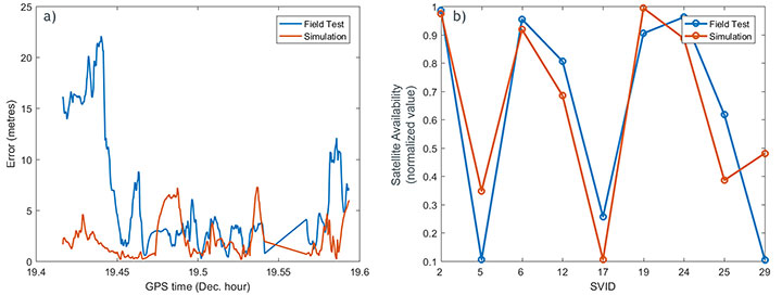
Figure 12a illustrates the positioning error obtained from simulated (red) and field test (blue). The first part of the simulation produced an error smaller than the one obtained from field data. However, from the time 19.48, a good agreement can be seen. The satellite availability is also shown in Figure 12b. This last result was obtained with the improved model described in Figure 9.
Figure 12. (a) Positioning error for field-test (blue) and simulation (red); (b) satellite availability for field data (blue) and simulation (red) after scene improvement. (Image: Tommaso Panicciari, Mohamed Ali Soliman and Grégory Moura)
CONCLUSIONS AND FUTURE WORK
A new real-time system for multipath simulation is designed to generate realistic multipath that depends on time, position and type of urban environment. The 3D scene is used to calculate the multipath (reflection and diffraction) caused by the buildings and objects around the antenna.
Some first results demonstrated that realistic multipath can be generated by simulating reflections and diffractions even with a simple 3D model. However, the inclusion of finer details in the model can improve the simulation and make it even closer to reality.
As always, simulation interest is a tradeoff between reliability in all conditions and efforts to adapt (that is, to specify) a generic and simple model. The added value of our model consists in its simplicity and its good compliance with field data.
Ray-tracing techniques coupled with geometrical optics and uniform theory of diffraction are efficient and simple methods to simulate the propagation of GNSS signals in complex urban environments. Their efficacy is demonstrated by a good agreement between simulation and field measurements. Some discrepancies still exist and are due to the limitations of such a model:
The accuracy of the model is never perfect and, as ray-tracing is a deterministic method, the returned results strongly depend on the quality of the input data used to generate the model.
Geometrical optics is a simple (but efficient) method. Only specular rays are modeled, thus the system won’t be able to generate all the signals coming from other phenomena such as scattering. Another limitation is given by the hardware. In fact, the number of simulated multipath depends on the number of available channels in the simulator.
The simulation parameters try to mimic the field conditions. However, the simulated trajectory is approximated, and other factors like pedestrian motion, vegetation (isolated trees or forest) and traffic may contribute to reduce some of the discrepancies that can be observed between simulation and field
All of these limitations can explain the differences between simulated and measured data. Currently, the impact of vegetation (forest and/or isolated trees) models, pedestrian motion and traffic on the multipath signal can also be simulated and their performances are under evaluation.
ACKNOWLEDGMENTS
We thank Colin Ford and Ajay Vemuru from Spirent Communications and Antoine Boudet, Yann Dupuy, Arnold Duquesne and Paul Pitot from OKTAL Synthetic Environment.
MANUFACTURERS
The system described in this article consists of a Spirent GNSS simulator equipped with a SimGEN software suite and the SE-NAV simulator developed by OKTAL Synthetic Environment. SE-NAV is interfaced with SimGEN via the SimREMOTE protocol, a real-time control and motion API.
Tommaso Panicciari obtained a Ph.D. in telecommunications from the University of Bath (UK). He is a software/project engineer at Spirent Communications where his main activity focuses on spoofing and multipath simulation.
Mohamed Ali Soliman is completing a master’s degree in telecommunications with business at University College London. He is a product manager at Spirent Communications, managing multiple products including the multipath simulation offering.
Grégory Moura graduated from the French Institute of Aeronautics and Space with an M.S. in cosmology from Université de Toulouse. He manages the GNSS activities of the French company OKTAL Synthetic Environment.
The U.S. Department of Defense (DoD) and Israel’s Ministry of Defense are joining forces for the third time in setting up a startup competition to tap into new technologies to beat terrorism. More than $200,000 in prizes will be awarded to the most promising startups.
“As terrorists become ever more sophisticated, technological innovations become an increasingly critical component of detecting and defeating them,” challenge organizers said.
The challenge is is divided into two tracks.
The Urban Navigation Technologies Challenge focuses on navigating without GPS — an increasingly important issue for special forces, law enforcement and other anti-terrorism professionals who need to operate indoors or in environments where GPS is not available. (See more below.)
The General Technologies Challenge includes surveillance, social media analytics, image and video, cybersecurity, drones, robotics, personal protection, biometrics, reconnaissance, and detection of explosives or water contamination.
Both tracks are open to all startups, entrepreneurs, and research groups worldwide, with a deadline of March 9. Entries will be reviewed by an international panel of judges from the DoD, Israel Defense and other organizations.
The most promising startups will be invited to present at the Combating Terrorism Technology Conference in Tel Aviv University on June 17.
Navigation Challenge
Entries in Urban Navigation Challenge might include location services based on beacons, technologies incorporating pre-loaded maps, technologies that estimate a user’s position via dead-reckoning or step-counting, and any other technology for navigating or positioning with no GPS.
Technologies may include: laser, inertial, vision, simultaneous localization and mapping, dead reckoning, pre-installed beacons or other infrastructure, pre-loaded maps, Wi-Fi, cellular or any other solution that operates in a GNSS-denied environment.
The winning startup will receive a $100,000 prize and a runner-up receives $10,000.
In addition, Navigation Challenge finalists will demonstrate their technologies in a dedicated urban navigation test facility in Israel.