“Seen & Heard” is a monthly feature of GPS World magazine, traveling the world to capture interesting and unusual news stories involving the GNSS/PNT industry.
Researchers in Alaska tracked the migration patterns of olive-sided flycatcher birds by attaching tracking devices to them to discover why their population is declining. The songbirds travel more than 15,000 miles every year to South America and then back to Alaska. To survive the long trips, they require safe locations to rest during their journeys. The researchers believe the stopover sites may provide an answer to the declining population. During the five-year study, the researchers deployed 95 devices and recovered only 17. The data pointed to 13 stopover sites between Washington and Peru as well as their wintering areas in South America.
Crime ring members caught
Image: hdagli/E+/Getty Images
Members of an organized crime ring in the Florida Keys who are accused of stealing more than $2.5 million in boating navigation devices have been arrested, reported Local 10.com and Fox 4. Eleven men have been accused of targeting multiple marinas throughout Florida and stealing navigation devices from boats, specifically Garmin devices. For example, a Garmin 8612 H16 Model can be sold for more than $5,000. Ten suspects are in custody and are facing more than 122 charges.
A new study published in Science used tracking devices on 43 animal species during the 2020 COVID-19 lockdowns to find that wild animals emerged from their natural habitats and ventured closer to the roads and cities that were empty. The study used several methods to analyze tracking data. Researchers examined how much animals moved on an hourly basis and during a 10-day period. Across species and countries, on average, hour-to-hour movement was 12% lower in the spring of 2020 compared to the same period in 2019. With the end of lockdowns, human activity returned to normal, and animals had to adapt again. The results of the study demonstrate how humans can change their own behavior to lessen their impact on animals.
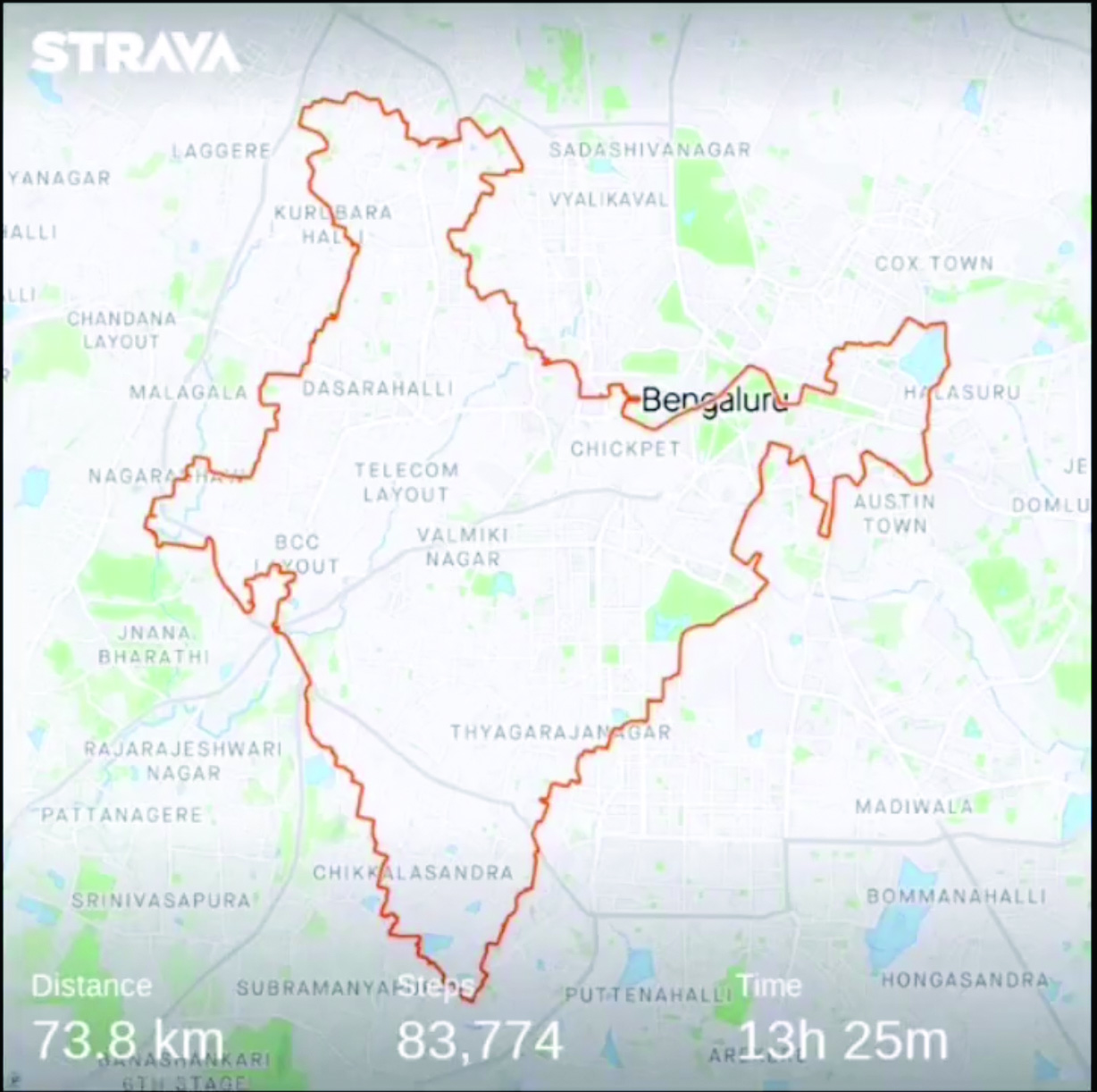
Navigation meets creativity
Image: @vikas_ruparelia on Twitter
A man from Bengaluru, India, Vikas Ruparelia, used the Strava navigation app to trace the country of India to celebrate its Independence Day. Ruparelia started and ended his journey at the Mahatma Gandhi statue near Orion Mall in Rajajinagar, India. He covered more than 73 km on foot in 17 hours. The Strava app enables users to track their running and hiking routes as well as join challenges. The route Ruparelia took was designed by another user of the app.
“Seen & Heard” is a monthly feature of GPS World magazine, traveling the world to capture interesting and unusual news stories involving the GNSS/PNT industry.
Image: Dennis Laughlin/iStock/Getty Images Plus/Getty Images
GNSS records Alaska earthquake data
Researchers in Alaska were able to compare the quality of GNSS and seismic station data when assessing the magnitude 8.2 Chignik earthquake near Dillingham, Alaska. Research recorded by Revathy Parameswaran and colleagues at the University of Alaska, Fairbanks, shows that GNSS and acceleration seismic data can be used interchangeably or in tandem to estimate rapid magnitude or ground motion. The research showed the Chignik earthquake velocity records were almost identical at co-located GNSS and seismic stations for observations at frequencies of less than 0.25 Hz.
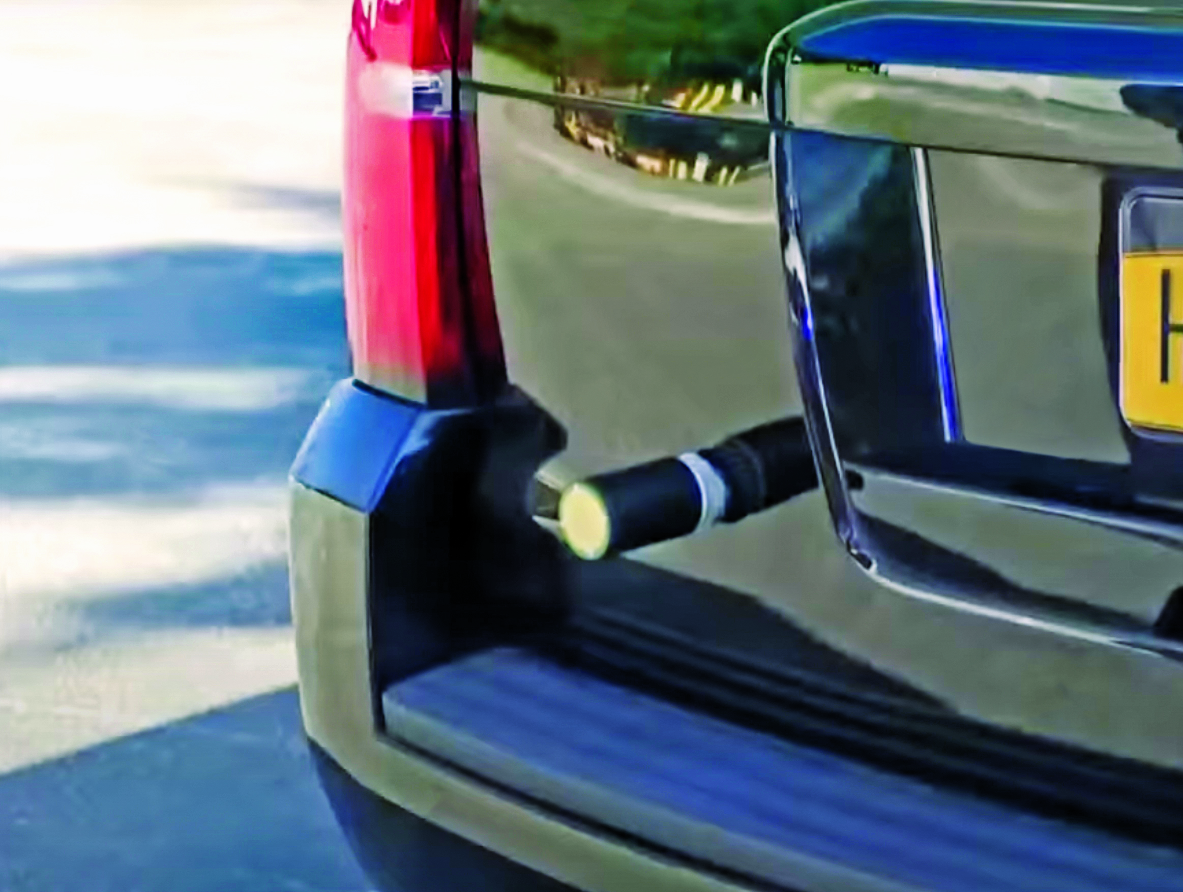
No more high-speed chases
Image: Screenshot from CBS New York video
The Old Westbury Police Department of Long Island, New York, has chosen a high-speed pursuit alternative — GPS-equipped darts that relay the current location of suspects, reported CBS New York. It took $36,000 to equip six patrol cars with the air-powered dart launcher, called StarChase, which can be activated from inside the patrol car. When the launcher is activated, it shoots onto the suspect’s vehicle a dart with a GPS receiver inside and an adhesive exterior. It is considered a safe alternative to high-speed chases and safe to use around pedestrians.
Shou Zi Chew, CEO of the popular app TikTok, testified before Congress that TikTok does not collect precise location data from its users. During the hearing, which lasted for more than five hours, Chew assured committee members the app does not collect nor distribute location data. TikTok is under fire as a bipartisan Senate proposal is aimed at banning the social media app, arguing it poses cybersecurity risks. The House Committee interrogated Chew regarding the app’s algorithmic feed, policies for young users and — given TikTok’s Chinese ownership — the amount of access the Chinese government has to user data.
Just some water, please
Image: Bob Douglas/iStock/Getty Images Plus/Getty Images
Satellite mapping data analyzed at Graz University of Technology’s Institute of Geodesy has revealed long-term drought conditions in Europe, reported GIM International. The data confirmed groundwater levels have been low consistently since 2018. The drought situation was originally published by Eva Boergens in “Geophysical Research Letters” in 2020 when she noted there was a severe water shortage in Central Europe during the summers of 2018 and 2019. There has been no significant rise in groundwater levels since then, and groundwater levels have stayed constantly low.
NV5 Geospatial has mapped more than 26 million acres of North America’s shoreline and riverine environments across more than 200 projects.
The projects have spanned from the Nuyakuk River in Alaska, Lake Tahoe in California, the Rio Grande in Texas, the entire coasts of South and North Carolina, the Achigan River in Quebec, Chesapeake Bay in Maryland and the Florida Keys.
In 2022, the company mapped and acquired topobathymetric lidar data for 14 projects including the Yellowstone River, Wyoming; Hells Canyon, Indiana; Revillagigedo Island, Alaska and Iles de la Madeleine in Quebec.
NV5 Geospatial first mapped these environments in 2012 using high-resolution bathymetric lidar and natural color imagery. The company mapped 34,051 acres of shoreline along the Sandy River, located in northwestern Oregon, to study the ever-changing basin geomorphology.
NV5 has also signed a two-year contract with the National Geodetic Survey of the National Oceanic and Atmospheric Administration to provide topobathymetric lidar, 4-band imagery and mapping of 3,115 sq miles of the Maine shoreline.
“For a decade we have been helping local, state, and federal government agencies as well as commercial and private entities gain the insights they need to solve some of their most challenging nearshore and riverine projects through our mapping technologies including topobathymetric lidar,” Kurt Allen, vice president of NV5 Geospatial, said. “Whether it be mapping the shoreline after a hurricane, updating the national shoreline, assisting water boards with flood planning, or hundreds of other possible use cases, we are constantly improving our technology and scalability to always be at the ready for our customers.”
Feb. 4 saw the news networks alive with sometimes wild reports about UFOs, UAVs and then a balloon. Balloons are used for weather forecasting on a regular basis, launched daily into the stratosphere with payloads gathering wind speed and direction, temperature, humidity, pressure and, of course, position.
Synchronized twice a day at about 900 locations around the world, balloons are released into the stratosphere gathering essential atmospheric data to feed our weather forecasts. Reaching altitudes of 20 miles, these balloons often drift on winds as far as 125 miles from the release point, broadcasting measurements from their onboard sensors.
At first, maybe North American Aerospace Defense Command (NORAD) thought the balloon crossing into Alaska’s airspace was just one of these high-altitude weather prediction vehicles. Aircraft were apparently scrambled, and initially it was decided there was no threat, so the balloon was allowed to continue and enter Alaskan airspace. It was detected and subsequently tracked by both the United States and Canada for some time as it continued to drift on the jet stream over the border into the lower 48. Then, people in and around Billings Montana (home to one of the nation’s three nuclear missile silo fields at Malmstrom Air Force Base) started to send in reports of a very large balloon high overhead — according to one observer with a high-resolution camera, it even seemed to be stationary for 35 minutes.
Apparently, by the time the good folks in Montana were looking up, the Pentagon had decided the balloon was a Chinese surveillance vehicle. To get this detail, one or more U-2 high altitude reconnaissance aircraft had been dispatched to investigate. The collected U-2 information spotted markings of a Chinese manufacturer on the 200-foot-tall balloon. A payload the size of a small passenger jet dangled some 20 feet below the balloon canopy. It had several antennas of various configurations. A huge solar panel was attached — presumably to power its suite of surveillance sensors.
The Federal Aviation Administration (FAA) ordered a ground stop for all aircraft traffic at the Billings airport while decisions were made about downing the balloon or allowing it to proceed.
Meanwhile, it may seem obvious that both the United States and China have developed, launched and make use of surveillance satellites. I imagined that a couple of dozen of these space vehicles would be buzzing over not only each other’s landmass, but also surveilling dozens of other countries as they orbit the whole planet.
What I found was a report that China had at least 260 such orbital observation platforms in 2022, and the United States has even more. Isn’t that enough without resorting to lower-tech balloons?
It’s possible that some electronic transmissions are short range and would not be detected by surveillance satellites operating in geosynchronous orbit (22,000 miles out), or even at 300 miles where the International Space Station (ISS) and most surveillance satellites hang out. So, a slow-moving balloon at 20 miles up might be ideal to “sniff” ground transmissions from sensitive military installations, and if you could control the balloon to hover, all the better to pick up radio signals. Could the gathering of transmission data somehow be used to geo-locate the source? It’s something the U.S. military may be working on, too, as it is reportedly also building a fleet of autonomous dirigibles and balloons.
According to press reports, the United States decided not to immediately take down the balloon, even though it subsequently discovered its surveillance capabilities. Not only was there concern over debris falling on populated areas but allowing the balloon to continue its flight over the United States provided an opportunity to observe its behavior and gather useful information. U.S. bases along its path apparently shut down all communications in sequence, as the balloon passed overhead.
The balloon was apparently found to be transmitting – presumably reporting on where it was and what it had detected. But, at some time transmissions ceased, possibly when U.S. Air Force activity was detected nearby.
The take-down off Myrtle Beach
An F-22 flew to almost the same altitude as the balloon and fired an AIM-9X Sidewinder missile into it, leaving the payload to tumble from 60,000 feet into the shallow (50-foot deep) Atlantic Ocean off Myrtle Beach, South Carolina. Recovery boats were already on hand to pick up the collapsed canopy, and to begin locating the electronics payload on the seabed. At time of writing, the U.S. recovery effort has yet to inform us on finding the key electronic payload, which would go a long way to confirming the intended mission for the balloon.
Image: Screenshot of CNN news coverage
Strange, but a couple of days later over Canada, F-22s were again in action to take down a “cylindrical object” detected at 40,000 feet — an altitude posing a danger to airline traffic. Little has been released on what this object might have been — could it possibly be a re-entering piece of space debris? Again, debris recovery and analysis is underway, and we patiently wait for a public report about what this was all about.
What have we learned?
Both China and the United States operate huge fleets of surveillance satellites gathering intelligence daily about each other’s capabilities and those of other countries. Both China and United States have also invested in surveillance balloons, but China is the only country to send one over U.S. territory.
There may have been earlier balloon incursions, which are only now being reported. The U.S. response was initially to determine the configuration of the balloon and its payload, then to allow its journey along the jet stream to continue. The United States has said the balloon did not uncover anything already available by other means, but recovery and analysis of the payload would presumably confirm this announcement.
China is not happy about the U.S. takedown of a harmless, stray weather balloon. And what the heck were F-22s shooting at in Canada?
We’ll tell you more when we learn more….
Tony Murfin
GNSS Aerospace
Editor’s Note: Since the initial instance of an unidentified object floating across U.S. airspace — later identified as a Chinese surveillance balloon — three additional unidentified aerial objects were spotted in North American airspace. One was spotted in Alaska, one in northern Canada and one over the Great Lakes region. All three were shot down by U.S. fighter jets out of caution.
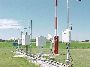
My April column addressed the vertical movement at the NOAA CORS Network (NCN). The values at the sites indicate the potential movement of marks in the area of the CORS. The rates are based on GNSS data and have an estimate of error associated with them.
As I mentioned in my previous column, I’m not sure how the National Geodetic Survey (NGS) will address the vertical movement effects in the new, modernized National Spatial Reference System (NSRS). That said, NGS will be monitoring the CORS and looking for trends to help describe the vertical movement at the CORS. These trends are an indication of what may be happening in that area.
As stated in previous columns, orthometric heights in NAPGD2022 will be defined through ellipsoid heights and a geoid model, for example GEOID2022. In addition to the movement of individual marks due to crustal movement, there are geophysical reasons for changes in the geoid that affect the orthometric height of a mark. Therefore, changes in the geoid model will be very important to users estimating orthometric heights using GNSS.
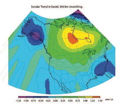
As stated in the NOS NGS 64 report, NGS has set a goal of maintaining geoid accuracy at 1 centimeter (1 standard deviation) in both absolute and differential geoid undulations. The box titled “Figure 13 from NOS NGS 64 Report” depicts an estimate of the secular change in the geoid. As indicated in the plot, the changes are very small, ranging from -1.25 mm/year to 1.5 mm/year.
What I find interesting is the small negative change in the southeastern United States. There are other drivers for geoid changes. This column will address some of these changes and what they mean to users.
Secular geoid change
Figure 13 from NOS NGS 64 Report (Image: NGS)
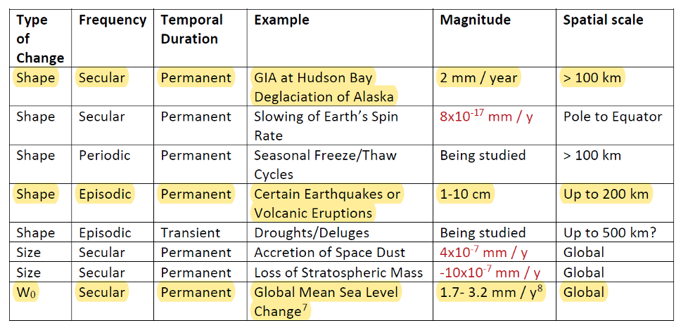
As mentioned in many of my articles, the new, modernized NSRS has a time-dependent component. This includes the geoid model. Table 5-1 from NOS NGS 64 report are examples of some of the physical processes being investigated by NGS to account for changes in the geoid. (See the box titled “Some of the geophysical drivers of geoid change.”)As mentioned in the NOS NGS 64 report, the magnitudes in red have already been determined to be too small for NGS to model. The examples highlighted in yellow have magnitudes that are significant and NGS will attempt to account for these changes to the geoid.
Table 5-1: Some of the geophysical drivers of geoid change
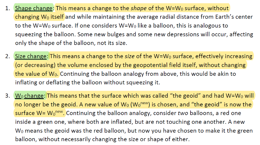
NGS classifies the changes in the geoid in three different groups: Shape Change, Size Change, and W0 Change. The box titled “The Groups of Geoid Change” provides NGS’s definition and explanation of the terms.
The groups of geoid change
NGS’s report on their Geoid Monitoring Service (GeMS) program provides figures that depict an estimate of the secular geoid rate trend based on the NASA GSFC mascon model. See the boxes titled “Estimate of Geoid Rate Over CONUS” and “Estimate of Geoid Rate Over Alaska.” For more details on GeMS, download the report NOAA Technical Report NOS NGS 69: A Preliminary Investigation of the NGS’s Geoid Monitoring Service (GeMS), and read my December 2019 Survey Scene column. The secular geoid rate trend is an example of the geoid changing its shape, but not the W0 value. What this means is that the local geoid undulations will change, but the overall size of the geoid will not.
Estimate of geoid rate over CONUS
Figure 32: Geoid rate over CONUS based on the GSFC mascon model [mm/yr] (Image: NOAA)Estimate of geoid rate over Alaska
Figure 33: Geoid rate over Alaska from GSFC mascon model [mm/yr] (Image: NOAA)These changes in the geoid are fairly small values (+/- 1.3 mm/year), but they will accumulate over a decade. As previously stated, NGS’s goal is to maintain geoid accuracy at the centimeter level (1 standard deviation) in both absolute and differential geoid undulations. In my February 2022 column, I discussed how coordinates change because Earth’s surface is moving due to the movement of major tectonic plates. It’s fairly obvious how the tectonic shift affects horizontal coordinates, but earthquakes and volcanic eruptions can also cause large shifts in vertical coordinates.
In recent history, on May 18, 1980, geologists watched in awe as Mount St. Helens erupted in a gigantic explosion. After the eruption, the volcanic cone of Mount St. Helens had been completely blasted away; the peak, which was at an elevation of 9,677 feet (2,950meters) was changed to a horseshoe-shaped crater with an elevation of 8,363 feet (2,549 meters). Extreme crustal movements such as the Mount St. Helens eruption can change the shape of the geoid. As explained in my April 2022 newsletter, NGS understands this and is attempting to manage the changing coordinates by providing a time-dependent component to a mark’s ellipsoid height, but there is also a time-dependent component to the geoid that affects the mark’s orthometric height.
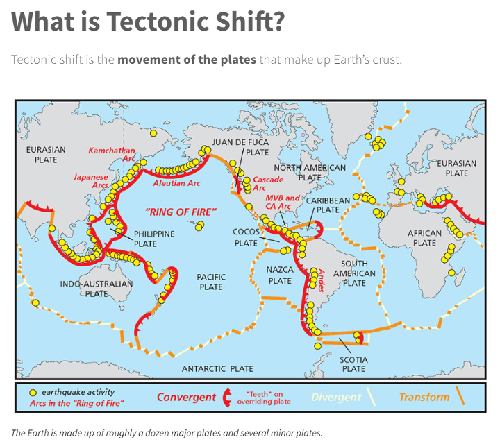
Ring of Fire
Image: National Ocean Service
The “Ring of Fire” map highlights earthquake activities around the world. As indicated in Table 5.1, earthquake or volcanic eruptions can change the shape of the geoid. Of course, they also can change the height of a mark due to crustal movement, which would typically be larger than the change in the geoid height. The amount of movement would be due to the size and magnitude of the event, but even small earthquakes could cause a change in the height of a mark located near the event. Earthquakes are occurring all over the world every day.
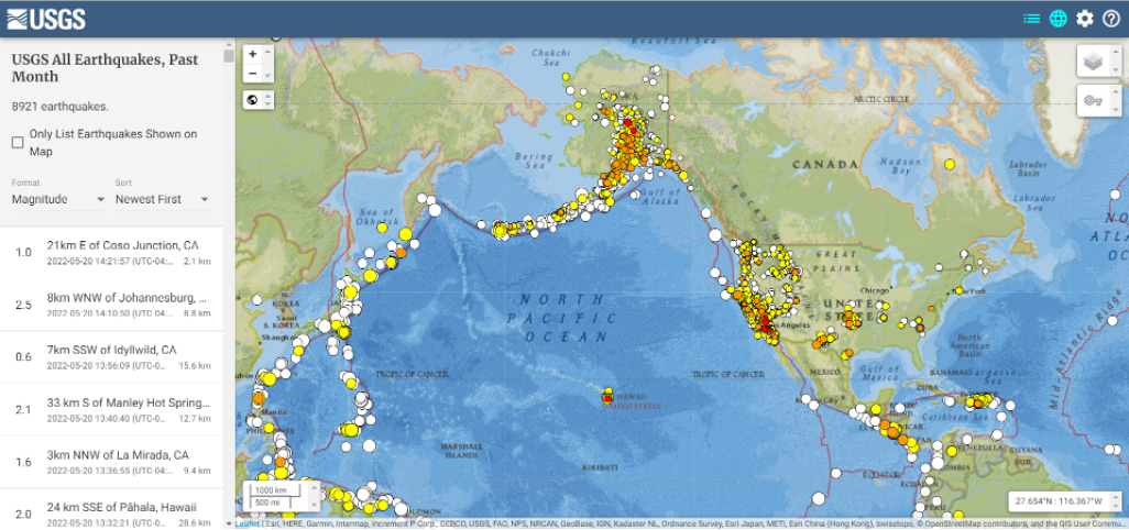
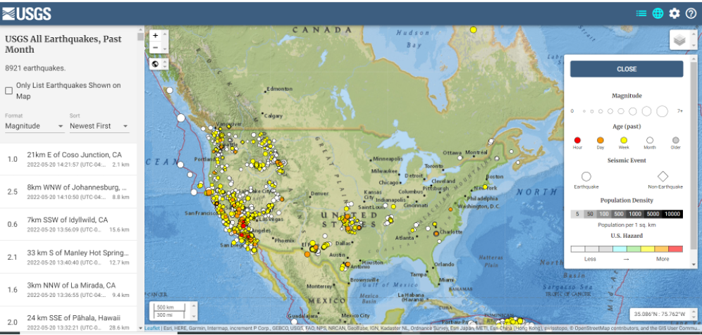
Earthquakes with large magnitudes are highlighted by news media outlets, but ones with smaller magnitude typically are not highlighted. The four figures below provide examples of earthquakes that have occurred over 30 days. This information can be obtained from the United States Geological Survey (USGS).
Earthquakes during the past 30 Days Date: May 20, 2022
Image: USGS
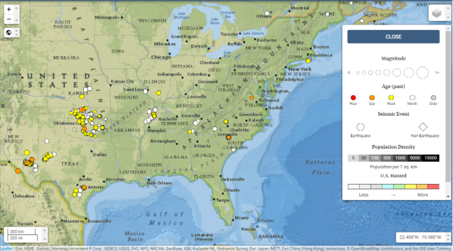
Earthquakes in the lower 48 during the past 30 days Date: May 20, 2022
Image: USGS
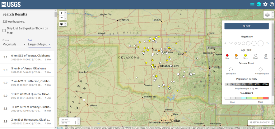
Earthquakes in eastern United States in the past 30 days Date: May 20, 2022
Image: USGS
I found the large number of earthquakes that occurred in Oklahoma in just 30 days to be very interesting. This isn’t something that I thought occurred in the eastern region of the United States.
Earthquakes in Oklahoma during the past 30 days
Date: May 20, 2022
Image: USGS
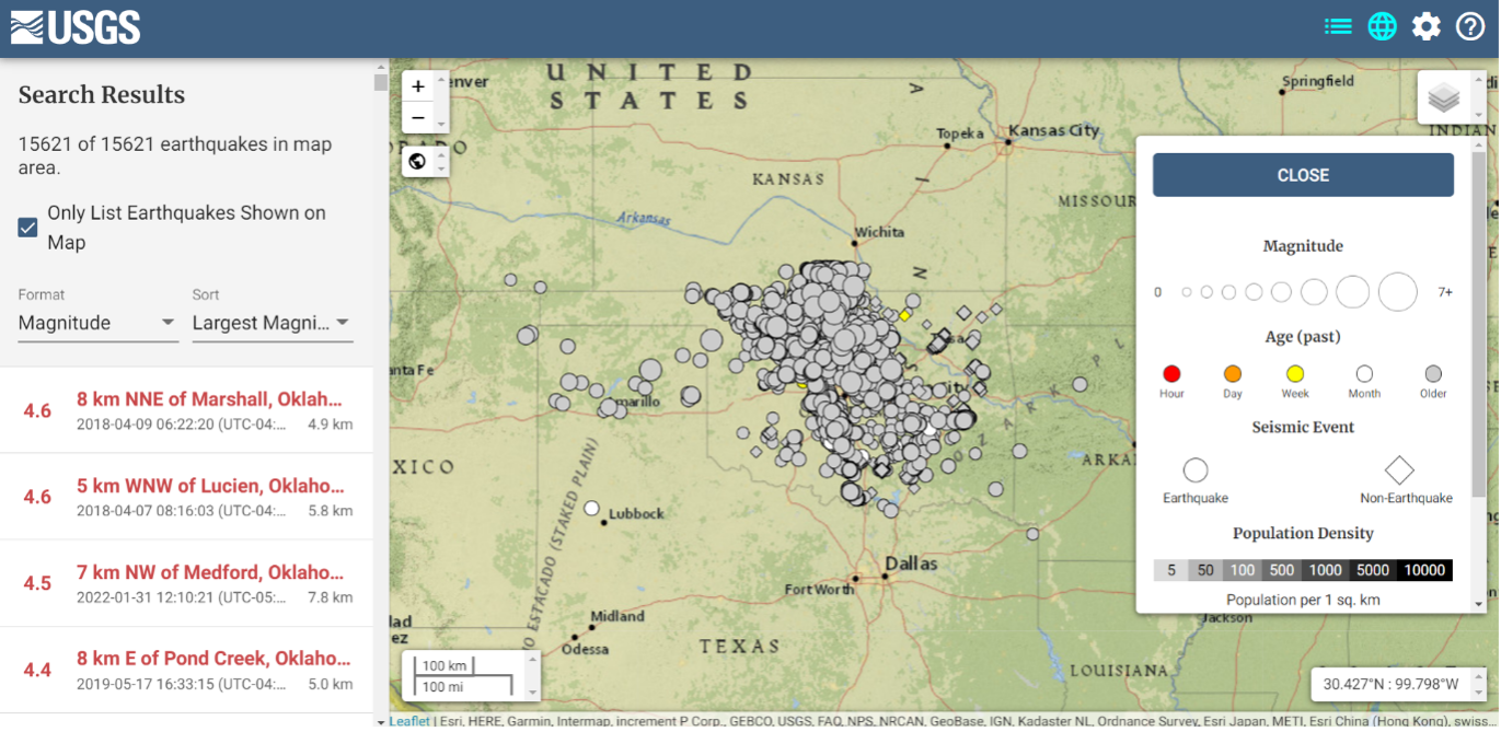
The image below depicts earthquakes that have occurred in Oklahoma in the past five years. They are fairly small in magnitude, but what is the cumulative effect on the geoid in the region, as well as changes to the orthometric heights of marks due to crustal moment in the region? This is why it is important for the new, modernized NSRS toimplement time-dependent coordinates.
Earthquakes in Oklahoma in the last 5 years Dates: 2017 to 2022
Image: USGS
To better understand the changes to the geoid, NGS performed a survey in Alaska to obtain geodetic data as part of its GeMS program. On May 12, 2022, Kevin Ahlgren, a geodesist at NGS, described in a webinar the observations collected and some of the results.
The presentation provided an overview of a field campaign performed in support of the GeMS program and a time-dependent geoid model. The campaign included static GNSS, relative gravity, and deflection of the vertical techniques on 50 stations in Alaska. The webinar was can be downloaded.
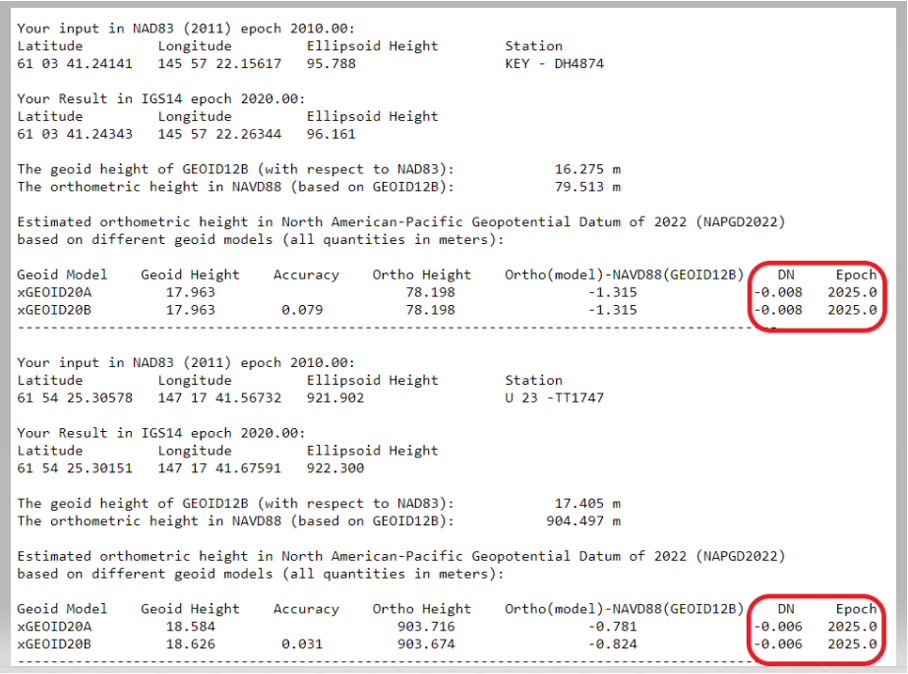
I encourage everyone to download the presentation. The change in the geoid due to geophysical drivers is small, but if the new, modernized NSRS is going to include time-dependent coordinates, then changes in the geoid must be accounted for. For demonstration purposes, NGS provides an example of the time-dependent geoid change in the xGEOID20 webtool. The box below, “xGEOID20 interactive computation output,” is an example of using this tool. The two stations are located in Alaska. As indicated in the output from the tool, the change in the geoid is 8 mm in five years. Again, NGS’s goal is to maintain geoid accuracy at the centimeter level (1 standard deviation) in both absolute and differential geoid undulations. These small changes can become significant over time.
xGEOID20 interactive computation output
Note: DN is the time-dependent geoid change computed between user inputted epoch (t) and t. (Image: NGS)
The last geoid change group that I’ll highlight has to do with the change in the gravity potential (W0) value that defines the model. The NOS NGS 64 Report states that the standing definition of the geoid, as adopted and used at NGS, is the following:
The geoid is the equipotential surface of the Earth’s gravity field which best fits, in a least squares sense, global mean sea level.
As stated in the NOS NGS 64 report, over a century of sea-level measurements imply that global mean sea level (GMSL) was rising at a rate of approximately 1.7 millimeters per year and was rising at a rate of 3.2 millimeters per year between 1993 and 2010 (IPCC, 2014). If NGS is going to define the geoid as theequipotential surface of the Earth’s gravity field that best fits, in a least squares sense, global mean sea level, then the geoid in the new, modernized NSRS must change when the GMSL exceeds a certain threshold.
Again, NGS’ goal is to maintain geoid accuracy at the centimeter level (1 standard deviation) in both absolute and differential geoid undulations. What this means is that as GMSL rises, the value of gravity potential which best fits to GMSL (called W0) will also change. In other words, the surface which was called “the geoid” and had W=W0in 2022 will no longer be the geoid. A new value of W0 (W0new) is chosen, and “the geoid” would now be the surface W=W0new.
So, what does this really mean to users? The NOS NGS 64 Report states on page 37:
“NGS and the Canadian Geodetic Survey have jointly adopted the value of 2.0 m^2/s^2 as the replacement threshold for a new geoid model (and new geopotential datum). This represents approximately 20 centimeters of GMSL (and thus geoid) rise. At the current rate of sea-level change of about +3 millimeters per year (IPCC, 2014), this means NGS expects to replace NAPGD2022 in approximately 60 to 70 years.”
Therefore, this should not be a major concern of users for a long time.
This column highlighted that orthometric heights in NAPGD2022 will be defined through ellipsoid heights and a geoid model, for instance GEOID2022; and therefore, changes in the geoid model will be very important to users estimating orthometric heights using GNSS. It briefly described the geophysical reasons for changes in the geoid that affect the orthometric height of a mark.
If NGS is going to meet the goal of maintaining geoid accuracy at 1 centimeter (1 standard deviation) in both absolute and differential geoid undulations, they will have to address changes in the geoid. The secular changes in the geoid, as indicated in Figure 13 in the NOS NGS 64 report, are very small, ranging from -1.25 mm/year to 1.5 mm/year. Once again, these are small changes to the geoid, but they will accumulate over time, and that is why NGS is including time-dependent coordinates in the new, modernized NSRS.
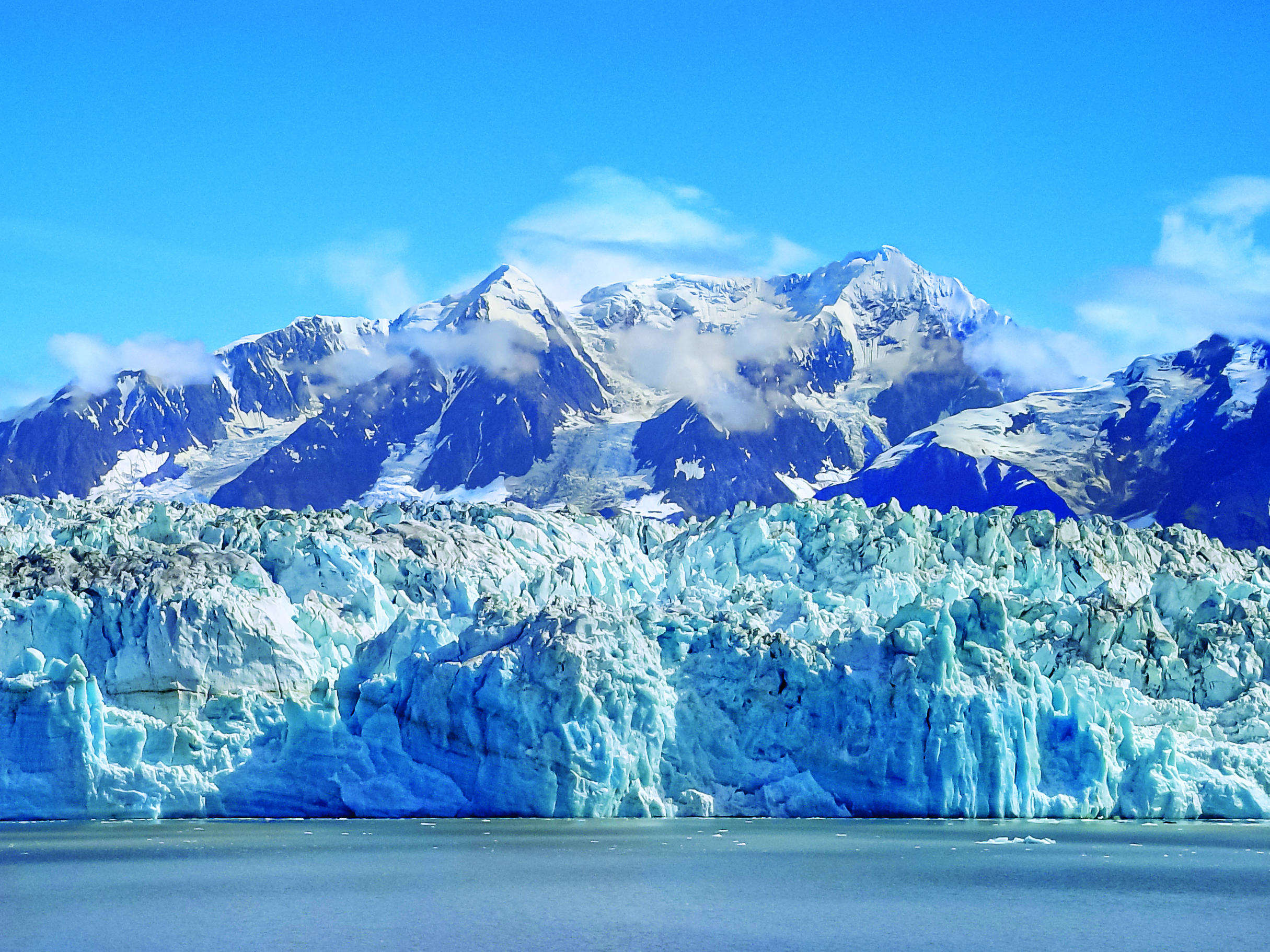
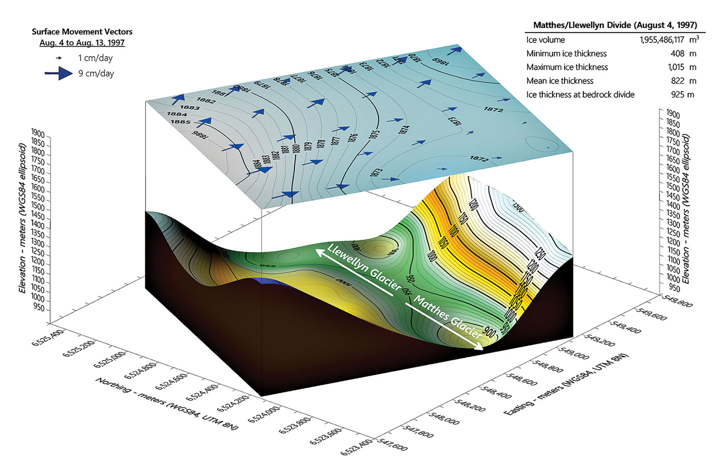
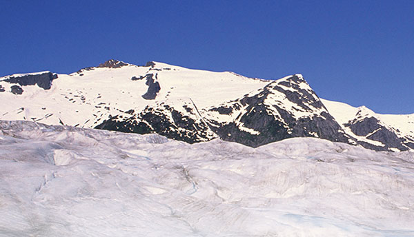
The Juneau Icefield Research Program (JIRP) calculates that thinning of Alaska’s Taku Glacier has increased from an average rate of 0.5 meter to 2 meters per year over the past two decades. Annual mapping by JIRP reveals the glacier’s thickness has varied from one year to the next, likely due to snow accumulation variability, but the overall current trend shows an annual net loss of ice.
“Taku is losing enough meltwater every day to fill an NFL stadium,” said Seth Campbell, JIRP director of Academics & Research.
At more than 800 square kilometers, Taku Glacier is the largest in the massive Juneau Icefield, making it vital to the study of climate change.
JIRP monitors the complex kinematics and mass balance of the Juneau Icefield — changes to ice velocity, snow accumulation and surface melting — to estimate whether the glacier is advancing or retreating over time. The team maps yearly GPS field measurements in Golden Software’s Grapher and Surfer modeling packages.
Image: JIRP/Golden Software
Straddling the Alaska-Canada border, the receding icefield plays multiple important roles in local ecosystems. For British Columbia, it provides fresh water, but for the Gulf of Alaska, increasing glacier meltwater can potentially harm the marine ecosystem and valuable fisheries.
JIRP research dates from 1946; the introduction of GPS in 1993 contributed significantly to annual summer fieldwork. Volunteers capture more than 1,000 GPS measurements at designated transect locations on the icefield each year to record glacial velocity and surface elevation changes.
Using Grapher, the team plots GPS “Z” elevation values across transects in 2D to generate thickness profiles. The scientists also input GPS field points for multiple transects from multiple years into the Surfer 3D surface mapping package to gain a sense of overall glacier volume change.
The primary revelation from the JIRP work has been a greater understanding of how and where the glaciers are changing, according to Scott McGee, JIRP Geomatics Program Lead. Until recently, glacial melt was assumed to occur mostly at lower elevations of the icefield, where temperatures are generally higher. However, McGee and the JIRP team have routinely discovered thinning occurring at all elevations of the icefield, including at the highest elevations of 1,900 meters.
The contract begins the offering for the purchase of complete drone solutions to all state agencies, commissions, political subdivisions, institutions and local public bodies allowed by law.
DroneUp is an end-to-end drone pilot service provider for aerial data collection. In August 2019, the company was awarded the Unmanned Aerial Systems (UAS) Services Master Agreement #E194-79435 by the Commonwealth of Virginia.
The services under this latest award (Contract Number #2020DRONE0002) are available for use by all 50 states, the District of Columbia, and the territories of the United States through the National Association of State Procurement Officials (NASPO) ValuePoint Cooperative Purchasing Organization.
The State of Alaska is now able to use the award for the benefit of state departments, institutions, agencies, political subdivisions, and other eligible entities.
DroneUp’s award includes but is not limited to service categories for
Emergency Support Services,
Law Enforcement Support,
Aerial Inspection or Mapping Data Services,
Agricultural and Gaming, and
Agency Media Relations and Marketing.
Primary users are expected to be
Agriculture & Game Management,
Emergency Management,
Transportation,
Forestry,
Mines,
Minerals and Energy, and
Public Universities and Community Colleges.
“We appreciate the efforts to streamline public sector access to leading-edge UAS services through the contract with the State of Alaska, and we look forward to supporting our hardworking state and local agencies,” said Tom Walker, DroneUp’s CEO.
The GPS Week Number Rollover, which took place April 6, has caused several automated NOAA stations to go offline.
Some of the outages could last until November.
Photo: NOAA
According to the EOS website, 19 National Oceanic and Atmospheric Administration (NOAA) coastal and marine automated stations were not updated to mitigate the issue, and those stations are out of commission until workers can service them on location.
The New York Times is reporting that at 7:59 p.m. EDT on Saturday, the New York City Wireless Network went dark, interrupting functions such as the collection and transmission of information from some Police Department license plate readers, Department of Transportation traffic-light programming, and communications at remote work sites for the sanitation and parks departments.
The city is now working overtime to bring affected systems back online, reports StateScoop.
Previously, GPS World reported on rollover issue for the Australian Bureau of Meteorology’s (BOM) weather balloons, as well as Boeing aircraft. Read more about the Boeing issue here.
Fairweather crew lower a launch into Puget Sound, Washington, for Hydrographic Systems Readiness Review testing. (Photo: NOAA)
U.S. researchers have completed the first high-resolution, comprehensive mapping of one of the fastest moving underwater tectonic faults in the world, located in southeastern Alaska.
The mapping information will help communities in coastal Alaska and Canada better understand and prepare for the risks from earthquakes and tsunamis that can occur when faults suddenly move.
Since 2015, scientists have been gathering data on the Queen Charlotte-Fairweather fault system, a 746-mile long strike-slip fault line that extends from offshore of Vancouver Island, Canada, to the Fairweather Range of southeast Alaska.
Team members are from the National Oceanic and Atmospheric Administration (NOAA), the U.S. Geological Survey (USGS) and their partners.
The most recent survey came from NOAA ship Fairweather, with USGS scientists aboard from April through July, when it collected multi-beam bathymetric data in an area along the U.S. and Canadian international border in water depths ranging from 500 to more than 7,000 feet deep.
Researchers aboard NOAA Ship Fairweather collected multibeam bathymetric data in an area along the U.S. and Canadian international border in water depths ranging from 500 to more than 7,000 feet deep from April through July. (Image: USGS)
“Providing scientific information to help protect vulnerable communities is one of our most important missions,” said W. Russell Callender, assistant NOAA administrator for the National Ocean Service. “Working with USGS and our state and academic partners, allows us to speed the development of information that can help communities better anticipate and prepare for risks from tsunamis and earthquakes.
“This project has been a great collaboration on an important scientific issue with significant implications for public safety,” said David Applegate, USGS associate director for natural hazards. “We will apply what we learn from this mapping mission to hazard assessments for Alaska’s coastal communities. Partnering with NOAA reflects the importance of addressing earthquake and associated tsunami hazards to both our missions, and it enables the USGS to bring our geologic expertise to bear on offshore fault structures that have significant onshore implications.”
Fault line activity poses a hazard to the growing populations of Juneau, Sitka and other communities throughout southeastern Alaska, as well as more than a million annual tourists and the seafloor infrastructure critical for Alaska’s communications and offshore energy industries.
With a slip rate of more than 2 inches per year, this fault may be one of the fastest-moving strike-slip faults in the world. (For comparison, the San Andreas fault in central California slips about an inch to an inch-and-a-half each year.)
Movement between the tectonic plates at the fault line has generated six earthquakes of magnitude 7 or greater within the last century. One of those earthquakes, a magnitude 7.8 earthquake near Lituya Bay, Alaska, in 1958 triggered a landslide that sent water 1,720 feet up an adjacent mountainside, one of the highest recorded run-ups of a tsunami — a rapidly rising turbulent surge of water often choked with debris.
A NOAA survey ship uses its multibeam echo sounder to conduct hydrographic surveys. (Image: NOAA)
A series of large-magnitude earthquakes and associated aftershocks in 2012 and 2013 spurred research cruises in 2015, in the first systematic effort to study the offshore Queen Charlotte-Fairweather fault system in U.S. territory in more than three decades.
A similar effort led by the Geological Survey of Canada has been underway along the portion of the fault located in Canadian territory.
The 2018 Fairweather survey built on five previous USGS-led marine geophysical and geological surveys between 2015 and 2017 in southeastern Alaska aboard a number of research vessels, as well as two cruises led by researchers from the Geological Survey of Canada, Sitka Sound Science Center and USGS.
During these surveys, researchers used an array of instruments to collect data on seafloor depth and texture, to profile sedimentary layers beneath the seafloor, and to derive sediment ages.
NOAA Ship Fairweather underway in Alaska. (Photo: NOAA)
NOAA nautical charts will be updated with the Queen Charlotte Fault data within a year once the data goes through a standard quality control process — although the fault area is too deep for any obstructions to pose a threat to marine traffic.
This research is part of a larger two-year effort between the NOAA Integrated Coastal and Ocean Mapping Program and USGS to map large portions of the Cascadia continental margin in federal waters offshore of Alaska, California, Oregon and Washington.
Polaris Wireless, a provider of high-accuracy, software-based wireless location solutions, has signed a multi-year, multi-phase contract for delivery of a wireless location solution that complies with the Federal Communications Commission’s (FCC) most recent E911 wireless location accuracy mandate with The Alaska Wireless Network, a company wholly owned by GCI Communication Corp (GCI).
The first phase of the contract extension includes the Polaris Wireless Evolved Serving Mobile Location Center (E-SMLC) with hybrid location software for LTE networks that complies with FCC-mandated indoor location requirements. Subsequent phases include delivery of additional location technologies and hybrid algorithms as cellular networks and mobile devices continue to evolve and become more capable.
Polaris Wireless describes its hybrid location solution as inherently future proof to take advantage of improvements in cellular networks and mobile devices.
“We are excited to continue working with GCI in providing our software-based location solutions,” said Amir Sattar, vice president of global operations for Polaris Wireless. “Polaris takes great pride in GCI trusting us to provide GCI E9-1-1 callers with the highest level of location accuracy when and where they need it most.”
“We have enjoyed a long-term relationship with Polaris Wireless delivering wireless E9-1-1 location solutions for many years,” said Gene Strid, chief technology officer of GCI. “As the carriers must now locate E9-1-1 callers in challenging indoor environments, we are happy to leverage Polaris Wireless’s technological innovation and commitment in delivering high-accuracy, software-based location solutions.”
“Polaris Wireless E-SMLC product leverages all available and emerging technology to deliver the best location position accuracy we can for our subscribers’ emergency calls,” said John Myhre, vice president of wireless technology at GCI.
The last column, February 2017, focused on addressing the following questions: (1) Is the large GPS on benchmarks residual due to an issue with the NAVD 88 orthometric height or the NAD 83 (2011) ellipsoid height? and (2) Should stations with large GPS on benchmarks residuals be included in the development of NGS’ hybrid geoid models? The column provided suggestions on how users can assist NGS in determining the reason for the large difference between the modeled hybrid geoid value and computed GNSS/leveling geoid computed value. It was mentioned that this information will be useful to NGS when developing hybrid geoid models and the 2022 Vertical Transformation model. My previous columns have focused on the conterminous United States. This column is going to discuss the GPS on benchmarks residuals for the state of Alaska.
The February 2017 column noted that many of these large GPS on BM residuals could be due to an invalid NAVD 88 published height because the benchmark moved since the last time the height of the benchmark was adjusted and published, and/or an undetected error in an ellipsoid height due to a weak GNSS project design. The State of Alaska is very large; it has a sparse leveling network, and benchmarks are subject to movement due to ground conditions, isostatic effects, and seismic activity. The Geophysical Institute at the University of Alaska, Fairbank, has a lot of interesting reports on the movement in Alaska. Many of these stations would be identified as benchmarks with invalid heights when users follow Federal geodetic survey guidelines, procedures, and specifications. Benchmarks with invalid heights would not be used in controlling geodetic surveys and, in my opinion, should not be used in the hybrid geoid model. As I mentioned in my previous columns, this is not meant to be a criticism of NGS process for creating their hybrid geoid model. NGS’ goal is to create a hybrid geoid model that is consistent with published NAVD 88 values. I believe NGS is using all the data and information available to them. A goal of my last column was to emphasize to users the importance to strategically occupy stations to help support the GPS on benchmarks program which will result in the creation of a hybrid geoid model that accurately represents the current NAVD 88.
First, let’s look at the leveling network design of Alaska. Figure 1 depicts the leveling network design used to establish heights in the NAVD 88. The figure indicates that most of the leveling data used in NAVD 88 was between 1965 and 1975. It should be noted that a major releveling project was performed in 1965 after the 1964 Good Friday Alaska Earthquake. There were some short leveling lines performed in the late 1980s and early 1991s. These data are now old and the question about whether the NAVD 88 height of the benchmark is still valid must be addressed.
Figure 1 – Vertical Control used to establish heights in the NAVD 88 General Adjustment – It should be noted that nearly all of the leveling in the 1960s were performed after the 1964 earthquake (figure from a presentation titled “Achieving Great Heights: Toward a Better Vertical Reference System in Alaska” by Michael Dennis (National Geodetic Survey) and David B. Zilkoski (Geospatial Solutions by DBZ), March 28, 2014, 48th Annual Alaska Surveying and Mapping Conference, Fairbanks, Alaska)
Alaska is prone to both episodic crustal motion (i.e. earthquakes) and the effects of long-term isostatic adjustment, which makes maintaining accurate vertical control difficult at best. (See figure 2 for a plot of earthquakes in Alaska). The 1964 Good Friday Alaska Earthquake, a magnitude of 9.2, changed heights as much as 8 feet. In addition to the initial damage at the time of the earthquake, there’s a post seismic vertical deformation movement that occurred. Suito and Freymueller (2009) provided a postseismic deformation model predictions for the 1964 earthquake [see box titled “Postseismic Velocity Predictions from Suito and Freymueller (2009)]”. An ArcGIS raster layer was developed using the grid values obtained from the website. Figure 3 is a plot of the vertical deformation model using Suito and Freymueller’s gridded dataset.
This page provides access to postseismic deformation model predictions for the 1964 earthquake. The model includes afterslip and viscoelastic relaxation (including the viscoelastic response to the afterslip), for the best-fit model derived by Suito and Freymueller (2009). That model includes a realistic slab geometry and a uniform asthenospheric relaxation time of 20 years. The full reference for the paper and the model is given below:
Suito, H., and J. T. Freymueller, A viscoelastic and afterslip postseismic deformation model for the 1964 Alaska earthquake, J. Geophys. Res., doi:10.1029/ 2008JB005954, 2009.
The model predictions are available in three different formats:
1. A text file, Suito_vel.enu.txt with east, north and vertical model predictions evaluated on a 0.25 degree grid covering all of Alaska.
2. A set of three netcdf grid files for use with GMT, for the east, north and vertical components. Interpolated values for any location can be generated easily with the GMT grdtrack program.
o East component: Suito_east.grd.
o North component: Suito_north.grd.
o Vertical component: Suito_vert.grd.
3. A MATLAB .mat file, visco_1964_SF2009.mat containing a structure with model velocity predictions at GPS sites in Alaska and the surrounding area.
Figure 3 – Post seismic Vertical Deformation Movement after the 1964 Alaska Earthquake (Suito, H., and J.T. Freymueller, “A viscoelastic and afterslip postseismic deformation model for the 1964 Alaska Earthquake, J. Geophy. Res,” ArcGIS raster layer was developed using grid values obtained from this website.The NGS (formally the Coast and Geodetic Survey) releveled the area effected by the earthquake in 1965. Today, leveling is very expensive so estimating new heights of benchmarks after earthquakes really needs to be accomplished using GNSS surveys. However, as stated in my first column, June 2015, GNSS surveys provide accurate ellipsoid height when the appropriate procedures are followed, but an accurate geoid height is required to estimate an accurate GNSS-derived orthometric heights. Therefore, the question that needs to be addressed is how accurate is the geoid model in Alaska. As described in the last column, the GPS on benchmarks program is one method of evaluating the GNSS/Leveling/Geoid combined system.
Saying that, Alaska’s system of NAVD88 benchmarks is based on old leveling data and, due to ground ice conditions and crustal movement, are subject to changes in heights. This makes it difficult to evaluate the geoid model in Alaska using published NAVD 88 heights. However, NGS’ GPS on benchmarks program can help to identify outliers and long wavelength trends between NAVD 88 heights and GNSS-derived orthometric heights. GPS on BMs residuals using the published GEOID12B values in the State of Alaska were generated using the data from the NGS’ website. I described these data and the process in my February 2017 column. Figures 4 through 6 depict the GPS on benchmarks residuals using the hybrid geoid model GEOID12B for stations in Alaska. It should be noted that only bench marks that had NAD 83 (2011) published coordinates and NAVD 88 published heights with the attribute of “Adjusted” were used in this analysis. This analysis does not include any OPUS results.
Figure 4 – GPS on Benchmark Residuals Using Geoid12B in the State of Alaska – {GPS on BMs Residual = [GEOID12B value – (NAD 83 (2011) ellipsoid height value – NAVD 88 orthometric height value)]}. The Residuals are Depicted by Symbols (units = cm)Figure 5 – GPS on Benchmark Residuals Using Geoid12B in the State of Alaska –{GPS on BMs Residual = [GEOID12B value – (NAD 83 (2011) ellipsoid height value – NAVD 88 orthometric height value)]}. The Value of the Residuals are Labeled (units = cm)Figure 6 – GPS on Benchmark Residuals Using Geoid12B in the Haines and Skagway, Alaska, Region {GPS on BMs Residual = [GEOID12B value – (NAD 83 (2011) ellipsoid height value – NAVD 88 orthometric height value)]}. (units= cm)Looking at figures 4-6, most of the GPS on BMs residuals using GEOID12B appear to be less than a couple of centimeters. There are several stations that have large outliers but this is seen in every State in the conterminous United States. The small residuals using GEOID12B doesn’t really tell us much because the large threshold level used by the NGS Geoid Team can mask some issues. This was demonstrated in my last column. Notice that figure 6 only shows two GPS on BMs residuals in the Haines and Skagway area of Alaska. This is an area where more GPS on BMs would be helpful to evaluate the geoid model.
As I’ve mentioned in my previous columns, the user should analyze the GPS on BMs stations using the latest experimental gravimetric geoid that includes the new airborne GRAV-D data, e.g. xGeoid16b. NGS has a website that enables users to compute geoid height values using the latest experimental gravimetric geoid model. All benchmarks in Alaska that had NAD 83 (2011) published coordinates were submitted as input to the NGS’ xGeoid16 website and the results were used to create a file of GPS on BMs residuals for the State of Alaska. An example of the output from the xGeoid16 website is provided in the box titled “Output from xGeoid16 Website.” NGS’ experimental geoid website was described in my October 2015 column.
It should be noted that the input to the xGeoid16 website was NAD 83 (2011) coordinates and the output was provided in the IGS08 reference frame; therefore, the xGeoid16b geoid heights are referenced to IGS08. The GPS on BMs residuals was computed using the formula GPS on BMs Residual = [xGEOID16b value – (IGS08 ellipsoid height value – NAVD 88 orthometric height value)]. Figure 7 is a plot of the GPS on BMs residuals computed using xGeoid16b geoid values, IGS08 ellipsoid heights, and NAVD 88 orthometric heights.
Figure 7 – GPS on Benchmark Residuals Using xGeoid16b in the State of Alaska – Referenced to IGS08 (units = cm) – {GPS on BMs Residual = [xGEOID16b value – (IGS08 ellipsoid height value – NAVD 88 orthometric height value)]}. Green Line Represents the Leveling LinesFigure 7 indicates that there is an obvious bias of about a meter between the GNSS-derived orthometric heights referenced to IGS08 and the NAVD 88. This bias is expected since these GPS on BMs residuals are referenced with respect to IGS08. This has been described in more detail in my December 2016 column, and depicted in a figure on the NGS website. A bias and trend from the GPS on BMs residuals was removed by performing a least squares best fit planar surface of the differences (basically solving for a bias and a North-South and East-West tilt). Figure 8 is a plot of the GPS on BMs residuals using xGeoid16b in Alaska were a bias and trend was removed from the original computed GPS on BMs residuals that are depicted in figure 7. These GPS on BMs residuals will be used to identify outliers and will be referred to as GPS on BMs residuals (with a trend removed) in the reminder of this column.
Figure 8 – GPS on Benchmark Residuals Using xGeoid16b in the State of Alaska – Referenced to IGS08 with a trend removed– {GPS on BMs Residual = [xGEOID16b value – (IGS08 ellipsoid height value – NAVD 88 orthometric height value)]}. (units = cm) – Green Line Represents the Leveling LinesThe large absolute difference and tilt are not concerning, it’s the large relative differences between closely-spaced stations that need to be identified and explained. Removing the bias and trend in the GPS on BMs residuals is useful in identifying large relative differences between neighboring stations.
Figure 9 is another plot of the GPS on BMs residuals using xGeoid16b with the trend removed using different symbology. The “up” blue arrows indicated a positive residual and a “down” red arrow indicates a negative residual. It’s not surprising to see both positive and negative residuals because a trend was removed from the residuals.
Figure 9 – GPS on Benchmark Residuals Using xGeoid16b in the State of Alaska – {GPS on BMs Residual = [xGEOID16b value – (IGS08 ellipsoid height value – NAVD 88 orthometric height value)]}. Referenced to IGS08 with a trend removed (units = cm) – “up” blue arrows indicated a positive residual and a “down” red arrow indicates a negative residualWhat should be noticed is that there are a lot of large negative and positive residuals. Figure 10 is a plot of the GPS on BMs residuals (with a trend removed) with residuals greater than +/- 20 cm labeled. It may be difficult to see in the plot but there are two residuals in the Hains and Skagway, Alaska, region (see right corner of figure 10). Both stations have large positive GPS on BMs residuals. What is important is that the relative difference between the two stations is also large, i.e., 42 cm (80.4 cm – 38.4 cm). We will address this difference later in this column.
Figure 10 – GPS on Benchmark Residuals Using xGeoid16b in the State of Alaska –– [GPS on BMs Residual = [xGEOID16b value – (IGS08 ellipsoid height value – NAVD 88 orthometric height value)]. Referenced to IGS08 with a trend removed (units = cm) – Residuals greater than 20 cm are labeled.As previously mentioned, investigating GPS on BMs with large relative differences between closely-spaced stations helps to identify outliers. Figure 11 is a plot of the GPS on BMs residual (with a trend removed) in the Matanuska-Susitna Borough, Alaska, region. There are several stations that are relatively close to each other (TT2213, TT2332, and TT2299) and have large relative GPS on BMs residuals. That is, the relative difference in GPS on BMs residuals between stations TT2313 and TT2332, 24 km apart, is -9.9 cm (-6.3 cm – 3.6 cm), and between stations TT2332 and TT2299, 19 km apart, the difference in GPS on BMs residual is -26.3 cm [-32.6 cm – (-6.3 cm)]. These stations have published NAVD 88 heights but should stations with large GPS on BM residuals be included in the development of NGS’ hybrid geoid models? At a minimum, other stations near these stations should be occupied with GNSS to help determine if other monuments in the area have moved in the similar manner.
Figure 11 – GPS on Benchmark Residuals Using xGeoid16b in the Matanuska-Susitna Borough, Alaska, Region – Large Difference between two relatively closely spaced stations (TT2313 and TT2332) – Referenced to IGS08 with a trend removed – {GPS on BMs Residual = [xGEOID16b value – (IGS08 ellipsoid height value – NAVD 88 orthometric height value)]}. (units = cm)Figure 2, a USGS plot of earthquakes in Alaska, highlighted the problems with maintaining reliable, accurate NAVD 88 orthometric heights in Alaska. Figure 12 is a plot of GPS on BMs residuals (with a trend removed) using xGeoid16b in the State of Alaska with an overlay of fault lines. The ArcGIS layer of fault lines was obtained from ArcGIS online layers. Looking at figure 12, it’s obvious that the heights of benchmarks in Alaska are probably being influenced by seismic activity. Figure 13 is a plot of the vertical velocity values at GNSS stations generated by UNAVCO’s GPS Velocity Viewer Program at this website.
Figure 12 – GPS on Benchmark Residuals Using xGeoid16b in the State of Alaska with an Overlay of Fault Lines – Residuals are referenced to IGS08 with a trend removed – {GPS on BMs Residual = [xGEOID16b value – (IGS08 ellipsoid height value – NAVD 88 orthometric height value)]}. (units = cm)Looking at figure 13, it is obvious that benchmarks that haven’t been releveled in the past 30 years could have been significantly influenced by crustal movement.
Figure 13 – Vertical Velocity estimated at GNSS Station in Alaska using UNAVCO’s GPS Velocity-Viewer Program: Figure generated from this website.
Figure 14 is the same plot as figure 11 with an overlay of the fault lines. Are these stations being influenced by crustal motion? Repeat measurements are needed to address this issue. There is a great opportunity to assist in the development and assessment of hybrid geoid models if researchers and others that are conducting campaign GNSS surveys with long static occupations share their results with NGS. NGS has a Regional Geodetic Advisory in Alaska that could help facilitate getting the appropriate information to NGS’ geoid team. Nicole Kinsman is the NGS Regional Geodetic Advisor for Alaska. Ms. Kinsman is very knowledgeable on National Spatial Reference System (NSRS) issues in Alaska. She was very helpful to me as I was preparing this column.
Figure 14 – GPS on Benchmark Residuals Using xGeoid16b in the Matanuska-Susitna Borough, Alaska, Region with an overlay of Fault Lines – Large Difference between two relatively closely spaced stations (TT2313 and TT2332) – Referenced to IGS08 with a trend removed – {GPS on BMs Residual = [xGEOID16b value – (IGS08 ellipsoid height value – NAVD 88 orthometric height value)]}. (units = cm)Figure 15 is a plot of GPS on BMs residuals in the Yukon-Koyukuk borough, Alaska, region. Notice that there’s a large difference between relatively closely-spaced stations TT3571 and TT3555, 22.6 cm (31.7 cm – 9.1 cm). Saying that, the plot also depicts all the fault lines around these stations. This is another example of how difficult it is to maintain reliable orthometric heights in Alaska.
Figure 15 – GPS on Benchmark Residuals Using xGeoid16b in Yukon-Koyukuk Borough, Alaska, region with an Overlay of Fault Lines – Large Difference between two relatively closely spaced stations (TT3571 and TT3557) – Referenced to IGS08 with a trend removed – {GPS on BMs Residual = [xGEOID16b value – (IGS08 ellipsoid height value – NAVD 88 orthometric height value)]}. (units = cm)Figure 16 is a plot of GPS on BMs residuals in the Haines and Skagway, Alaska, region, with an overlay of fault lines. Figure 10 highlighted that the two stations, TT0118 and TT8080, have a large relative difference (42 cm) but figure 16 indicates that the two stations lie between a couple of fault lines.
Figure 16 – GPS on Benchmark Residuals Using xGeoid16b in the Skagway, Alaska, Region with an Overlay of Fault Lines – Referenced to IGS08 with a trend removed – {GPS on BMs Residual = [xGEOID16b value – (IGS08 ellipsoid height value – NAVD 88 orthometric height value)]}. (units = cm)What does this mean to surveyors and mappers in Alaska? In my opinion, the new 2022 Vertical Reference Datum, denoted as the North American-Pacific Geopotential Datum of 2022 (NAPGD 2022) will help Alaskans maintain a vertical reference frame that’s reliable and traceable. Saying that, it is extremely important to know the relative accuracy of the geoid model used to establish GNSS-derived orthometric heights in NAPGD2022. NGS is performing projects to evaluate the relative accuracy of the gravimetric geoid model. The projects are known as Geoid Slope Validation Surveys. I would encourage the Alaska surveying and mapping community to develop plans to transition to the new NAPGD2022. Evaluation of the experimental gravimetric geoid model is critical to the implementation of the new 2022 datum and should be part of a transition plan. Performing a geoid slope validation project similar to NGS may be too expensive to be performed by Alaskans. However, Alaskans may be able to perform low budget geoid slope evaluation surveys. These surveys could include performing combined GNSS and leveling surveys to evaluate the relative accuracy of the gravimetric geoid model in areas that require accurate orthometric heights. Performing several of the gravimetric geoid evaluation surveys in major cities and/or areas that require accurate heights would help to facilitate the implementation of NAPGD2022.
These types of geoid evaluation surveys should also be performed in other areas of the country that are influenced by crustal movement. For example, the published NAVD 88 heights in southern Louisiana and other parts of the Gulf Coast of the United States are influenced by subsidence. NAPGD2022 will provide a more efficient and cost-effective way to maintain consistent orthometric heights. Once again, evaluating the relative accuracy of the gravimetric geoid model is critical to the implementation of NAPGD2022.
The Alaska Geologic Map shows the generalized geology of the state, each color representing a different type or age of rock. (Image: USGS)
A new digital geologic map of Alaska is being released today, providing land users, managers and scientists geologic information for the evaluation of land use in relation to resource extraction, conservation, natural hazards and recreation.
The U.S. Geological Survey (USGS) map gives visual context to the abundant mineral and energy resources found throughout the state in a detailed and accessible format.
“I am pleased that Alaska now has a state-wide digital map detailing surface geologic features of this vast region of the United States that is difficult to access,” said Suzette Kimball, newly confirmed director of the USGS. “This geologic map provides important information for the mineral and energy industries for exploration and remediation strategies. It will enable resource managers and land management agencies to evaluate resources and land use, and to prepare for natural hazards, such as earthquakes.”
“The data contained in this digital map will be invaluable,” said National Park Service Director Jonathan B. Jarvis. “It is a great resource and especially enhances the capacity for science-informed decision making for natural and cultural resources, interpretive programs, and visitor safety.”
“A better understanding of Alaska’s geology is vital to our state’s future. This new map makes a real contribution to our state, from the scientific work it embodies to the responsible resource production it may facilitate. Projects like this one underscore the important mission of the U.S. Geological Survey, and I’m thankful to them for completing it,” said Sen. Lisa Murkowski, R-Alaska.
This map is a completely new compilation, carrying the distinction of being the first 100 percent digital statewide geologic map of Alaska. It reflects the changes in our modern understanding of geology as it builds on the past. More than 750 references were used in creating the map, some as old as 1908 and others as new as 2015. As a digital map, it has multiple associated databases that allow creation of a variety of derivative maps and other products.
“This work is an important synthesis that will both increase public access to critical information and enhance the fundamental understanding of Alaska’s history, natural resources and environment,” said Mark Myers, Commissioner of Alaska’s Department of Natural Resources. “I applaud the collaborative nature of this effort, including the input provided by the Alaska Division of Geological and Geophysical Surveys, which will be useful for natural disaster preparation, resource development, land use planning and management, infrastructure and urban planning and management, education, and scientific research.”
Geologists and resource managers alike can utilize this latest geologic map of Alaska, and a lay person can enjoy the colorful patterns on the map showing the state’s geologic past and present.
More than other areas of the United States, Alaska reflects a wide range of past and current geologic environments and processes. The map sheds light on the geologic past and present. Today, geologic processes are still very important in Alaska with many active volcanoes, frequent earthquakes, receding and advancing glaciers and visible climate impacts.
“This map is the continuation of a long line of USGS maps of Alaska, reflecting ever increasing knowledge of the geology of the state,” said Frederic Wilson, USGS research geologist and lead author of the new map. “In the past, starting in 1904, geologic maps of Alaska were revised once a generation; this latest edition reflects major new mapping efforts in Alaska by the USGS and the Alaska state survey, as well as a revolution in the science of geology through the paradigm shift to plate tectonics, and the development of digital methods. Completion of this map celebrates the 200th anniversary of world’s first geologic map by William Smith of England in 1815.”
This map detail, of the Anchorage area, shows the city spread out on a plain of loose glacial deposits shown in yellow, and the bedrock making up the hillsides of Anchorage shown in green and brown. The rocks shown in green, called the Valdez Group, are sedimentary rocks formed in a trench 65 to 75 million years ago from thousands of undersea debris flows similar to the modern Aleutian trench where oceanic crust dives under continental crust (a subduction zone). The rocks shown in brown on the map are a chaotic mix of rock types called the McHugh Complex that were also formed about the same time, adjacent to this ancient subduction zone. Some time after deposition of the Valdez Group, hot fluids formed gold-bearing quartz veins; the veins were mined starting in the 1890’s. The rocks were pushed up, and attached (accreted) to North America through plate tectonic forces in the past 65 million years. The dotted line passing through the east side of Anchorage is the approximate trace of the Border Ranges Fault system, the boundary between the accreted rocks and the rest of the continent. This map detail, of the Anchorage area, shows the city spread out on a plain of loose glacial deposits shown in yellow, and the bedrock making up the hillsides of Anchorage shown in green and brown. The rocks shown in green, called the Valdez Group, are sedimentary rocks formed in a trench 65 to 75 million years ago from thousands of undersea debris flows similar to the modern Aleutian trench where oceanic crust dives under continental crust (a subduction zone). The rocks shown in brown on the map are a chaotic mix of rock types called the McHugh Complex that were also formed about the same time, adjacent to this ancient subduction zone. Some time after deposition of the Valdez Group, hot fluids formed gold-bearing quartz veins; the veins were mined starting in the 1890’s. The rocks were pushed up, and attached (accreted) to North America through plate tectonic forces in the past 65 million years. The dotted line passing through the east side of Anchorage is the approximate trace of the Border Ranges Fault system, the boundary between the accreted rocks and the rest of the continent. This map detail, of the Anchorage area, shows the city spread out on a plain of loose glacial deposits shown in yellow, and the bedrock making up the hillsides of Anchorage shown in green and brown. The rocks shown in green, called the Valdez Group, are sedimentary rocks formed in a trench 65 to 75 million years ago from thousands of undersea debris flows similar to the modern Aleutian trench where oceanic crust dives under continental crust (a subduction zone). The rocks shown in brown on the map are a chaotic mix of rock types called the McHugh Complex that were also formed about the same time, adjacent to this ancient subduction zone. Some time after deposition of the Valdez Group, hot fluids formed gold-bearing quartz veins; the veins were mined starting in the 1890’s. The rocks were pushed up, and attached (accreted) to North America through plate tectonic forces in the past 65 million years. The dotted line passing through the east side of Anchorage is the approximate trace of the Border Ranges Fault system, the boundary between the accreted rocks and the rest of the continent. (Image: USGS)


![Figure 32: Geoid rate over CONUS based on the GSFC mascon model [mm/yr] (Image: NOAA)](https://stage.globalpositioningnews.com/wp-content/uploads/2022/05/Geoid-rate-CONUS.jpg)
![Figure 33: Geoid rate over Alaska from GSFC mascon model [mm/yr] (Image: NOAA)](https://stage.globalpositioningnews.com/wp-content/uploads/2022/05/geoid-rate-alaska.jpg)


![[INSERT FIGURE 3] Figure 3 – Post seismic Vertical Deformation Movement after the 1964 Alaska Earthquake (Suito, H., and J.T. Freymueller, “A viscoelastic and afterslip postseismic deformation model for the 1964 Alaska Earthquake, J. Geophy. Res,” ArcGIS raster layer was developed using grid values obtained from website: http://www.gps.alaska.edu/jeff/SF2009_postseismic.html)](https://stage.globalpositioningnews.com/wp-content/uploads/2017/04/GPS_World_Newsletter_12_Fig_3.jpg)
![Figure 4 – GPS on Bench Mark Residuals Using Geoid12B in the State of Alaska – {GPS on BMs Residual = [GEOID12B value – (NAD 83 (2011) ellipsoid height value – NAVD 88 orthometric height value)]}. The Residuals are Depicted by Symbols (units = cm)](https://stage.globalpositioningnews.com/wp-content/uploads/2017/04/GPS_World_Newsletter_12_Fig_4.jpg)
![Figure 5 – GPS on Bench Mark Residuals Using Geoid12B in the State of Alaska –{GPS on BMs Residual = [GEOID12B value – (NAD 83 (2011) ellipsoid height value – NAVD 88 orthometric height value)]}. The Value of the Residuals are Labeled (units = cm)](https://stage.globalpositioningnews.com/wp-content/uploads/2017/04/GPS_World_Newsletter_12_Fig_5.jpg)
![Figure 6 – GPS on Bench Mark Residuals Using Geoid12B in the Haines and Skagway, Alaska, Region {GPS on BMs Residual = [GEOID12B value – (NAD 83 (2011) ellipsoid height value – NAVD 88 orthometric height value)]}. (units= cm)](https://stage.globalpositioningnews.com/wp-content/uploads/2017/04/GPS_World_Newsletter_12_Fig_6.jpg)

![Figure 7 – GPS on Bench Mark Residuals Using xGeoid16b in the State of Alaska – Referenced to IGS08 (units = cm) – {GPS on BMs Residual = [xGEOID16b value – (IGS08 ellipsoid height value – NAVD 88 orthometric height value)]}. Green Line Represents the Leveling Lines](https://stage.globalpositioningnews.com/wp-content/uploads/2017/04/GPS_World_Newsletter_12_Fig_7.jpg)
![Figure 8 – GPS on Bench Mark Residuals Using xGeoid16b in the State of Alaska – Referenced to IGS08 with a trend removed– {GPS on BMs Residual = [xGEOID16b value – (IGS08 ellipsoid height value – NAVD 88 orthometric height value)]}. (units = cm) – Green Line Represents the Leveling Lines](https://stage.globalpositioningnews.com/wp-content/uploads/2017/04/GPS_World_Newsletter_12_Fig_8.jpg)
![Figure 9 – GPS on Bench Mark Residuals Using xGeoid16b in the State of Alaska - {GPS on BMs Residual = [xGEOID16b value – (IGS08 ellipsoid height value – NAVD 88 orthometric height value)]}. Referenced to IGS08 with a trend removed (units = cm) - “up” blue arrows indicated a positive residual and a “down” red arrow indicates a negative residual](https://stage.globalpositioningnews.com/wp-content/uploads/2017/04/GPS_World_Newsletter_12_Fig_9.jpg)
![Figure 10 – GPS on Bench Mark Residuals Using xGeoid16b in the State of Alaska –– [GPS on BMs Residual = [xGEOID16b value – (IGS08 ellipsoid height value – NAVD 88 orthometric height value)]. Referenced to IGS08 with a trend removed (units = cm) – Residuals greater than 20 cm are labeled.](https://stage.globalpositioningnews.com/wp-content/uploads/2017/04/GPS_World_Newsletter_12_Fig_10.jpg)
![Figure 11 – GPS on Bench Mark Residuals Using xGeoid16b in the Matanuska-Susitna Borough, Alaska, Region – Large Difference between two relatively closely spaced stations (TT2313 and TT2332) - Referenced to IGS08 with a trend removed – {GPS on BMs Residual = [xGEOID16b value – (IGS08 ellipsoid height value – NAVD 88 orthometric height value)]}. (units = cm)](https://stage.globalpositioningnews.com/wp-content/uploads/2017/04/GPS_World_Newsletter_12_Fig_11.jpg)
![Figure 12 – GPS on Bench Mark Residuals Using xGeoid16b in the State of Alaska with an Overlay of Fault Lines – Residuals are referenced to IGS08 with a trend removed – {GPS on BMs Residual = [xGEOID16b value – (IGS08 ellipsoid height value – NAVD 88 orthometric height value)]}. (units = cm)](https://stage.globalpositioningnews.com/wp-content/uploads/2017/04/GPS_World_Newsletter_12_Fig_12.jpg)

![Figure 14 - GPS on Bench Mark Residuals Using xGeoid16b in the Matanuska-Susitna Borough, Alaska, Region with an overlay of Fault Lines – Large Difference between two relatively closely spaced stations (TT2313 and TT2332) - Referenced to IGS08 with a trend removed – {GPS on BMs Residual = [xGEOID16b value – (IGS08 ellipsoid height value – NAVD 88 orthometric height value)]}. (units = cm)](https://stage.globalpositioningnews.com/wp-content/uploads/2017/04/GPS_World_Newsletter_12_Fig_14.jpg)
![Figure 15 – GPS on Bench Mark Residuals Using xGeoid16b in Yukon-Koyukuk Borough, Alaska, region with an Overlay of Fault Lines – Large Difference between two relatively closely spaced stations (TT3571 and TT3557) - Referenced to IGS08 with a trend removed – {GPS on BMs Residual = [xGEOID16b value – (IGS08 ellipsoid height value – NAVD 88 orthometric height value)]}. (units = cm)](https://stage.globalpositioningnews.com/wp-content/uploads/2017/04/GPS_World_Newsletter_12_Fig_15.jpg)
![Figure 16 – GPS on Bench Mark Residuals Using xGeoid16b in the Skagway, Alaska, Region with an Overlay of Fault Lines - Referenced to IGS08 with a trend removed – {GPS on BMs Residual = [xGEOID16b value – (IGS08 ellipsoid height value – NAVD 88 orthometric height value)]}. (units = cm)](https://stage.globalpositioningnews.com/wp-content/uploads/2017/04/GPS_World_Newsletter_12_Fig_16.jpg)

