[SPONSORED CONTENT] With the NovAtel Application Suite, you can monitor the status of all your receivers during operations, including GNSS satellite tracking, positioning and even interference detection – all in one integrated software suite.
Whether you are integrating our GNSS receivers with your system, undertaking post-operation analysis, or monitoring real-time output from your receivers, the NovAtel Application Suite lets you make the most of our industry-leading technology.
Artificial intelligence (AI) has become part of the daily lexicon, and an endless stream of media reports assert that AI either has affected or will affect most aspects of human life. What is AI and what are its components? How is it being used in GNSS technology? What is the near-term potential of AI in GNSS/PNT? These are weighty, evolving questions for which this column attempts an initial synthesis.
AI definitions and descriptions vary widely. One general and broad definition from IBM (2025) is “Artificial intelligence (AI) is technology that enables computers and machines to simulate human learning, comprehension, problem solving, decision-making, creativity and autonomy.” The idea of thinking machines (Turing, 1950) and the term “artificial intelligence” were introduced in the 1950s (McCarthy, 2007). The 1960s and 1970s saw the development of neural networks. The 1980s brought advances in neural network training and deep learning. The 1990s saw rapid advances in computing power. Big data and cloud computing developments in the 2000s allowed for the management and analysis of large datasets. The 2010s brought deep neural networks/deep learning, and the 2020s have seen the introduction and flourishing of large language models.
This column primarily focuses on the impacts that AI is directly having and could potentially have on GNSS hardware and PNT solutions, including receiver signal acquisition, measurement processing, position estimation, integrity and mitigation of jamming and spoofing. Due to space limitations, it will limit discussion to topics such as GNSS-based sensor fusion, navigation system routing, application-specific customizations, etc., all of which are undergoing significant AI-related infusions. A suitable guide to consider is the list of tasks for which evolving AI approaches can outperform existing methods in meaningful and efficient ways. For example, in error modeling or optimal estimation, can AI-based techniques fill gaps in non- or only partially-deterministic processes?
Essential
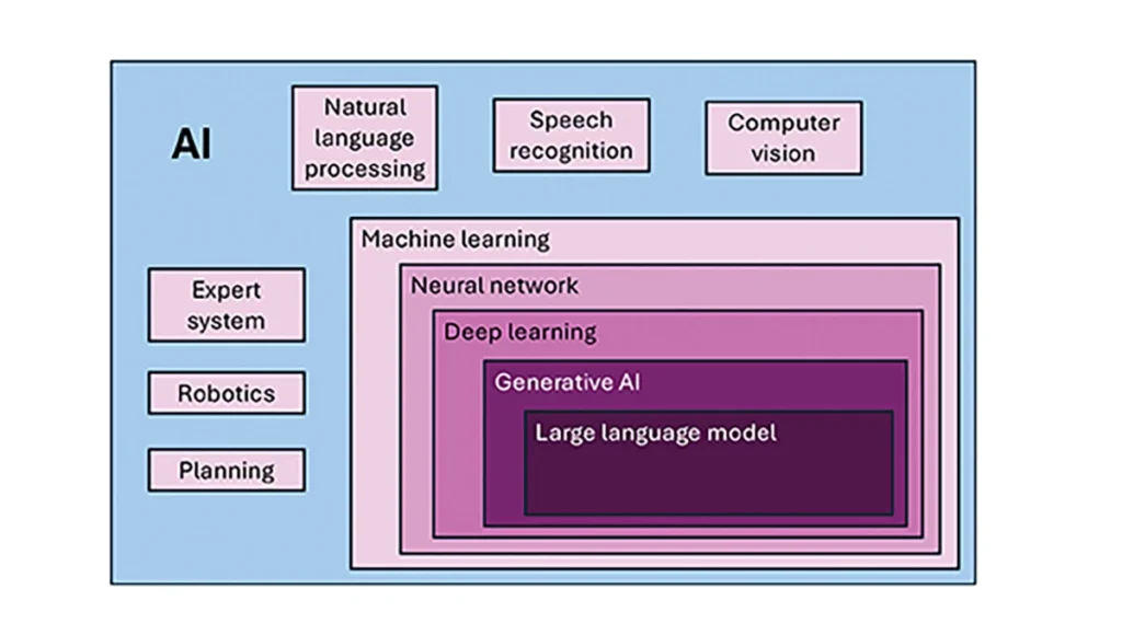
To investigate the current and potential uses of AI in GNSS, it is essential to define its components, especially as some terms are misused or conflated. The presented description is based on a wealth of Internet-based information, including from IBM (2025). Figure 1 illustrates the current broad concepts within, or subsets of, AI based on a synthesis of nomenclature used. In the figure, AI — defined here as a machine that exhibits human-like intelligence — is the superset. Within AI, there are many concepts or subsets that can be categorized, though they can overlap. There is perception intelligence, such as text and space recognition, and there is the broad area of machine learning.
Figure 1: Concepts within/subsets of AI.
Sophisticated processes have been developed and continue to rapidly evolve to give machines the ability to sense, learn and make decisions. Natural language processing (NLP) allows machines to recognize, understand and generate text following human language. Voice recognition is similar, in that the machine transcribes speech to text and back. Computer vision enables machines to interpret and analyze imagery. While robotics is a field of its own, within the superset of AI, it can be seen as an application of AI to motion. Planning refers to autonomously solving planning and scheduling problems. And expert system is the field of AI dedicated to simulating human expertise, judgment and behavior. All of these AI subsets are typically enhanced with machine learning (ML).
ML involves the development of algorithms and statistical models that can infer patterns (i.e., learn) from existing data without explicit instructions (i.e., rote training) and apply this knowledge to new data. Based on the learning approach, there are four types of machine learning algorithms: supervised, semi-supervised, unsupervised and reinforcement. (ML can also be classified by functionality.) Supervised learning uses manually labeled datasets to accurately train algorithms to classify data or predict outcomes. In semi-supervised learning and unsupervised learning, relationships are found with less or no explicit human interaction, respectively. Reinforcement learning combines these approaches with goal optimization. There are many types of ML techniques/algorithms, such as linear regression, logistic regression, decision trees, random forest, support vector machines, k-nearest neighbor and clustering, each designed for different types of problems and data.
Neural networks (NNs) or artificial neural networks are modeled after the human brain. A neural network model contains a given input layer and output layer, each with a set of nodes. These layers and nodes are interconnected with a set of hidden layers of nodes, with each node having a weight and bias, determined (i.e., estimated) based on the specified network inputs and outputs by utilizing one of a selection of optimization techniques. NNs can work well for tasks that involve identifying complex patterns and relationships given large amounts of data, though the details of specific parameter interrelationships cannot necessarily be determined by such models — therefore sometimes referred to as “black box” models. There are several types of neural networks, including convolutional NNs, long short-term memory networks, autoencoders, recurrent NNs, transformers, etc.
Deep learning refers to the depth of layers in a neural network. A deep learning model neural network contains at least three, but typically hundreds of hidden layers. Having many layers allows for unsupervised, fast and accurate identification of complex patterns and relationships. Generative AI can be described as deep learning models that generate new/original content, e.g., text, image or audio data through a variety of training, tuning and generation processes. Finally, large language models can read, understand and generate human language (refer to NLP), making use of all the functionality of ML.
Elements
How machine learning is used in GNSS
So, when should AI be used in GNSS/PNT tasks? A rudimentary answer is whenever AI can perform better (in some specified and measurable sense) than existing methods. The determination of this answer for a particular scenario requires research. From the descriptions of AI and its subsets, GNSS/PNT output is used in myriad AI applications such as sensor fusion, autonomous vehicle navigation, route planning, etc. However, it is primarily the ML subset of AI that is being researched for use in GNSS signal and measurement processing.
ML models can be categorized by their fundamental methodology, as either generative or discriminative, or by the tasks for which they are used: either regression or classification (IBM, 2025). Generative algorithms model the distribution of data points with the goal of predicting the joint probability of a data point appearing in a particular space, whereas discriminative algorithms model the boundaries between classes of data with the goal of predicting the conditional probability of a given data point being in a specific class. Regression models predict continuous values and are mainly used to determine the relationship between one or more independent variables and a dependent variable, whereas classification models predict discrete values and are mainly used to determine a category or class, e.g., binary or multi-class.
Siemuri et al. (2022) provide a comprehensive review of recent research (from 2020 through 2021) in which ML techniques are used in GNSS problem solving and provide a categorization of GNSS use cases. Relevant key findings include: 1) ML is proposed to increase GNSS/ PNT robustness under degraded signal environments; 2) more than 200 studies were assessed; 3) in most cases, the ML approaches outperformed (at varying levels of significance) the traditional GNSS models; and 4) industry adoption of ML in GNSS so far appears limited. The analysis found that neural networks were used in more than half of the studies (55%) — including some deep learning, while support vector machine and decision tree/random forest techniques were used in 19% and 10% of the studies, respectively. Use cases for machine learning in GNSS were categorized as: i) signal acquisition; ii) signal detection and classification; iii) Earth observation and monitoring; iv) navigation and positioning; v) denied environments and indoor navigation; vi) atmospheric effects; vii) spoofing and jamming; viii) GNSS/inertial integration; ix) satellite selection; and x) LEO satellite orbit determination and positioning.
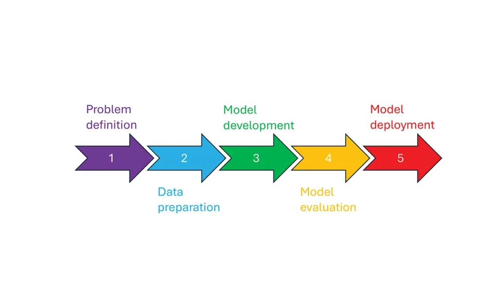
So, how is machine learning used in these GNSS/PNT use cases — and in general? How ML is applied can be described as a set of steps or a cycle with a varying number of components. Figure 2 presents a graphical synthesis from the literature, with a grouping of five core steps.
Step 1 — problem definition: understanding the problem(s) and goals, defining the available data, defining the problem inputs and outputs, determining the category of ML to use and selecting evaluation metrics.
Step 2 — data preparation: collecting the data, editing them, and labeling them if employing supervised classification.
Step 3 — model development: selecting the algorithm, selecting the model, building the model and training the model.
Step 4 — model evaluation: validating the model, tuning the model, analyzing the results, cross-validating the results and applying the evaluation metrics.
Step 5 — model deployment: finalizing the model, applying the model in prediction, and, if necessary, feeding back into the start of the cycle.
Figure 2 Steps in, or cycle of, machine learning implementation.
The scikit-learn (2025) library is a popular resource for Python-based ML information, tools and examples. An illustrative example of how ML can be used in GNSS for signal classification and measurement weighting is given by Li et al. (2023). The authors describe the process for designing the ML problem-solving scenario, selecting the models that are either of the regression or classification type and comparing the performance of many popular ML models to detect direct line-of-sight versus non-line-of-sight and multipath signals in urban environments. Note that most applications of machine learning in GNSS involve some form of supervised classification.
Initial and potential machine learning uses in GNSS
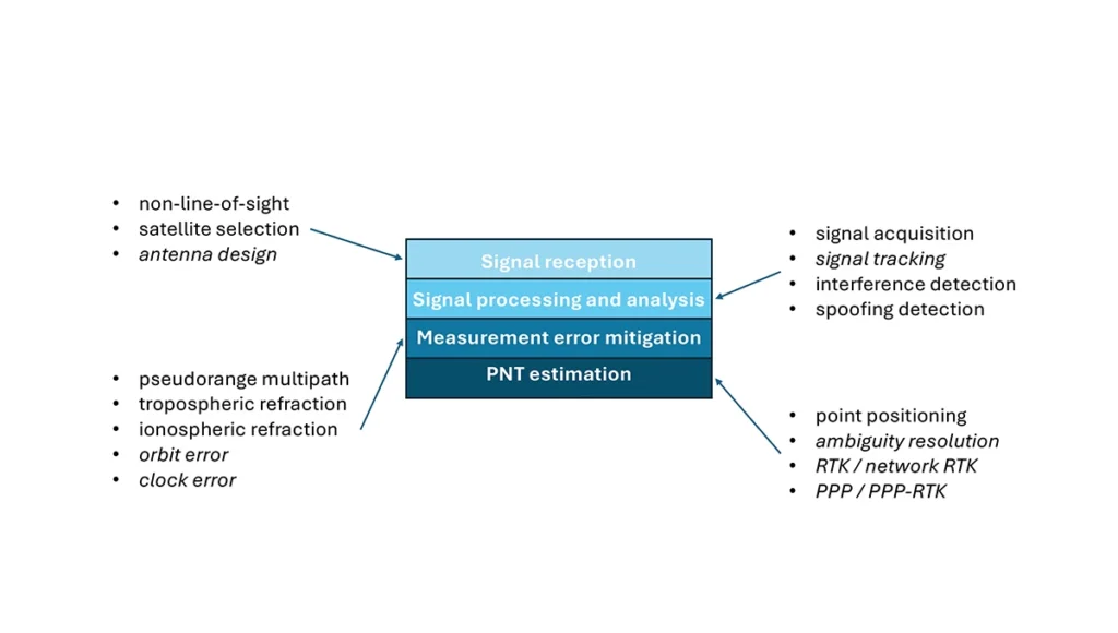
For this column, a brief synopsis is given of the use of machine learning in GNSS in the context of the application themes of signal reception, signal processing, measurement error mitigation and PNT estimation, as illustrated in Figure 3. Correspondingly, potential ML uses are also considered.
Figure 3: Application themes of machine learning in GNSS with initially studied and potential research areas.
Signal reception
Studies including Tsu (2017) and Li et al. (2023) have used various machine learning models to differentiate between line-of-sight, non-line-of-sight and pseudorange multipath GNSS signals in urban environments. Various input features, such as signal strength, are used to train models, resulting in majority accurate classification. ML has been used to optimize satellite selection (rather than using all available tracked satellites) for efficient PNT processing. Radio frequency hardware and software simulators can use ML to improve the realism of propagated signals in various environments and under different dynamics, including multipath, interference and spoofing. There is also the potential for ML to be used to improve antenna design, including for controlled radiation pattern antennas that generate one or multiple nulls.
Signal processing and analysis
Deep learning models have been used for signal acquisition and show improvement over current methods with simulated data (Borhani-Darian et al., 2023). There may be potential for the use of ML in signal tracking or in the design of new tracking algorithms and processes. Studies have shown that ML can be used to detect natural and intentional radio frequency interference. Various ML models have successfully been used to produce accurate classification of radio frequency interference jammer types (e.g., Morales Ferre et al., 2019). ML has also been used to detect signal spoofing with simulated and real signals with high levels of validation (e.g., Semanjski et al., 2020).
Measurement error mitigation
As GNSS multipath is a non-deterministic (and non-zero mean) process, it is a strong candidate for machine learning-based mitigation, especially meter-level pseudorange multipath (compared to centimeter-level carrier-phase multipath). Such studies, combined with non-line-of-sight classification, have been described in the previous section.
Initial investigations of the use of machine learning in the mitigation of tropospheric refraction appear promising (e.g., Łoś, et al., 2020). The wet tropospheric delay on GNSS signals is irregular, making it difficult to predict. Therefore, there is great potential for improved anomaly detection, refraction modeling and more accurate severe weather nowcasting.
As with tropospheric refraction, ionospheric refraction, while well understood, is difficult to model accurately, especially during periods of high solar activity. Machine learning has been shown to accurately detect anomalies and scintillation (e.g., Linty et al., 2018) and potentially for nowcasting.
There is the potential to improve GNSS satellite orbit and clock estimation with ML, as these are both well-defined processes, but also contain levels of process uncertainty. For example, it is usual to include once-per-orbital revolution empirical accelerations in orbit estimation states, and satellite force models can always be improved. Consequently, ML studies may aid in such GNSS network processing to improve the accuracy of real-time and post-processed correction products.
PNT estimation
Well-established optimal estimation techniques such as least-squares and Kalman filtering work extremely well for most GNSS/PNT estimation cases. However, hardware limitations and environmental conditions can lead to measurements not meeting the technical assumptions of these conventional approaches, e.g., the use of independent measurements, the absence of systematic errors, the absence of gross errors, the use of realistic measurement variances, etc. Deep learning models have the potential to improve GNSS point positioning (e.g., Kanhere et al., 2022) in test data, if poor model numerical conditioning, changing satellite visibility and model overfitting are managed. There is potential research in the use of machine learning methods to improve carrier-phase ambiguity resolution, and in the centimeter-level positioning techniques of real-time kinematic (RTK)/network RTK, and precise point positioning (PPP)/PPP-RTK.
Broader AI/ML use within GNSS-based PNT
Clearly, GNSS/PNT outputs are used in a broad spectrum of applications, for which AI and ML are currently being used or have the potential of being used to attain and enhance goals. Machine learning has been used to improve GNSS-derived position time series analysis for many Earth science applications, including in plate tectonics, tsunami monitoring, vulcanology, subsidence monitor, GNSS reference station monitoring, overall measurement integrity, etc. and in diverse GNSS-enabled techniques such as radio occultation and reflectometry (Siemuri et al., 2022).
ML has the potential to allow for improvements in sensor fusion, chief amongst these being GNSS/inertial measurement unit (IMU) integration. Improvements can be found in IMU calibration and in managing functional and dynamic mismodeling for specific user applications. Wider, multi-sensor fusion, such as for simultaneous location and mapping solutions, rely heavily on ML approaches, such as reinforcement learning.
Finally, GNSS-based PNT is used in most of the non-ML subsets of AI. GNSS-based position information is central to many outdoor robotics, planning and computer vision algorithms, providing either seeding localization information for other sensors or processes, or core position information for the overall AI-driven system.
Machine learning resource considerations
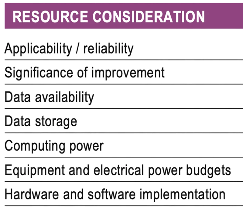
As with all technology, a cost/benefit analysis is required when considering the application of ML in a specific GNSS use case. Table 1 summarizes the broad considerations. Can the problem at hand be reliability mitigated with ML, in the sense that there are complexities that are difficult or impossible to physically model, but sufficient patterns in the data to be modeled by ML? If ML can outperform a conventional approach using specified metrics, is the improvement significant to the user? Are there large enough, i.e., sufficient and varied, datasets to train a model for prediction over expected data variations? As most ML algorithms require large amounts of computing storage for large datasets, typically from data servers, can the necessary computing power be brought to bear? Similarly, given that most ML algorithms require large amounts of computing power for myriad computational operations, typically utilizing graphics processing units (GPUs), is such computing power available? As storage servers for large datasets and GPUs for processing are expensive and require large amounts of electrical power, are the financial and electrical power, environmental and security resources available? And finally, how practical is it to implement the ML model on user equipment or via servers?
Table 1 Resource considerations for machine learning use in GNSS.
Evolutionary
AI is a broad field that is rapidly developing and entering service in most technologies. While AI includes many subsets such as computer vision, natural language processing and robotics, the ML subset (which includes neural networks, deep learning and generative AI) has the most direct applicability to GNSS/PNT. Of the available ML models used in GNSS, most are supervised (i.e., they use labeled training data), and the majority use neural networks. Initial studies of applications such as signal classification and interference detection indicate that supervised ML models perform better than traditional approaches.
Many subsets of AI, such as computer vision and robotics, rely heavily on ML, while GNSS/PNT has only recently seen investigations in ML use. For many applications, it can be that conventional deterministic models, physics-based models or optimal estimation techniques work well and reach desired performance standards. However, as GNSS/PNT continues to trend to lower cost hardware, harsher environmental conditions and increasing safety-of-life usage, PNT outliers and corner cases grow in importance, and ML can potentially provide solutions, as outlined in Figure 3. These are the early days of investigating and applying ML in GNSS/PNT. To use ML or not to use ML — that is the question. There are many factors to consider, as described in Table 1. Performance improvements over current approaches and operational practicality (i.e., costs) will dictate ML adoption. Much more research is required in many GNSS/PNT applications, followed by significant wide-spread testing and tuning of developed ML models. It is difficult not to predict the near-term adoption of ML in at least some GNSS/PNT use cases, if they will benefit our daily lives. Look for future columns that will examine and investigate ML implementations in specific GNSS/PNT applications that prove its efficacy.
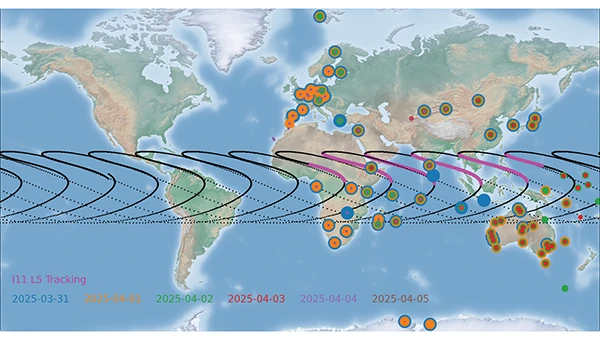
NVS-02 is a second-generation navigation satellite of the Indian regional navigation satellite system NavIC. It was launched on Jan. 28, 2025, but could not reach its designated orbit due to a malfunction of a valve of the thrusters. Thus, the satellite is still in its transfer orbit. As of April 2025, the NVS-02 perigee is about 190 km, whereas the apogee is 37,400 km above the Earth’s surface. The inclination is about 21° and the eccentricity is 0.74. The groundtrack of NVS-02 is illustrated in Figure 1 and currently has a repeat cycle of about six days.
As of today, starting on Feb. 19, 2025, a decent number of receivers of the International GNSS Service are tracking the L5 signal of NVS-02 with the pseudo-random noise number I11. The L5 tracking of dedicated stations on individual days is indicated by different colors in Figure 1. Although the groundtrack has global coverage, no stations in Northern and Southern America have tracked I11 so far. The tracking is limited to periods when the satellite is near the apogee with altitudes between 23,000 km and 37,400 km and visible from the Indian Ocean region. During these periods, indicated in pink in Figure 1, the transmitter is active and the antenna is roughly pointing toward Earth.
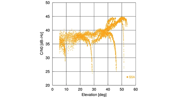
Figure 2 shows the carrier-to-noise density ratio (C/N0) of the NVS-02 L5 signal tracked by a Septentrio PolaRx5 receiver at the German Space Operations Center (GSOC) of the German Aerospace Center (DLR) in Oberpfaffenhofen, Germany. Sudden drops in the C/N0 occur at about 8°, 28°, 46° and 52°. Here, the line of sight to the satellite is at the edge of the transmit antenna main lobe with a significantly lower gain, introducing the drop in signal power and, finally, the loss of lock.
Figure 2: Elevation-dependence of the carrier-to-noise density ratio of the NVS-02 L5 signal at Oberpfaffenhofen, Germany. (All figures provided by the authors)
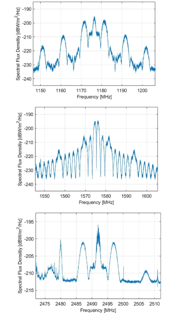
The spectral flux density of NVS-02 in the L5, L1 and S band is shown in Figure 3. The L-band spectra have been measured with GSOC’s 30 m high-gain antenna in Weilheim, Germany. As the feed of this antenna is limited to the L band, the S band spectrum has been recorded with a 5 m dish antenna of DLR’s Institute of Communication and Navigation.
Figure 3: Spectral flux density of NVS-02 in the L5 (top), L1 (middle) and S band (bottom). (All figures provided by the authors)
The peak in the L5 spectrum at the center frequency of 1176.45 MHz is related to the civil Standard Positioning Service and introduced by a Binary Phase Shift Keying (BPSK) modulation with 1 MHz bandwidth. The two broader peaks with an offset of 5 MHz from the center frequency are caused by a Binary Offset Carrier (BOC) signal of the Restricted Service with a bandwidth of 2 MHz. Sidelobes of that signal are visible at the center frequency ±15 MHz and ±25 MHz.
For the L1 band, a Synthesized Binary Offset Carrier (SBOC) is used. It consists of two BOC signals with 1 MHz bandwidth and offsets of 1 MHz and 6 MHz, respectively. The two mainlobes of the BOC (1,1) component are visible at 1575.42±1 MHz, and the mainlobes of the BOC (6,1) component at 1569 MHz and 1581 MHz. The same type of signals, as in L5, are transmitted on the S band carrier with a center frequency of 2492.028 MHz. Due to its different location in a less remote area, compared to the 30 m antenna in Weilheim, the 5 m antenna in Oberpfaffenhofen suffers from pronounced interference with other signals in the S band; the most prominent peak can be seen at 2480 MHz, several smaller and sharper peaks over the whole frequency range shown in the lower plot of Figure 3. Possible causes of these interferences are WiFi and civilian and military radiocommunication services.
Although NVS-02’s mean orbit height is steadily decreasing due to the atmospheric drag around the perigee, the satellite will stay in orbit for at least a decade. However, navigation signal transmission might stop at any time due to operational constraints or unfavorable conditions in the non-nominal orbit.
[SPONSORED CONTENT] On April 10, 2025, Mike Horton, project creator of GEODNET, testified before the U.S. Congress on behalf of both GEODNET and the broader DePIN (Decentralized Physical Infrastructure Networks) ecosystem. The testimony showcased how blockchain-powered DePINs are already delivering scalable, cost-effective infrastructure across essential sectors such as internet connectivity, precision navigation, and renewable energy.
This milestone reflects growing recognition from U.S. policymakers and affirms the real-world value and momentum behind decentralized technologies. A proud moment—and a powerful motivator for everyone working to build the future of infrastructure.
Merriam-Webster defines a “silver bullet” as a magical weapon, one that instantly solves a long-standing problem. Well, it’s been about 30 years. Despite studies, analyses, tests, demonstrations and much hand-wringing, no silver bullet technology has been identified to back up the myriad GPS dependencies that now permeate U.S. critical infrastructure (CI).
The President, members of Congress, Deputy Secretaries and the President’s National Space-Based PNT Advisory Board have all weighed in to insist that such a backup be put in place to preserve the operational continuity of domestic CI, all to no avail. As a participant in or observer of virtually all these efforts over the past 20 years, I am as familiar with and frustrated as anyone by the lack of progress or urgency.
Now, the Federal Communications Commission (FCC) is the latest to join the fray in late March with a public hearing preceded by a Notice of Inquiry (NOI) on Promoting the Development of PNT Technologies and Solutions, as well as a separate but related Notice of Proposed Rulemaking on improving wireless E911 location accuracy. As with many of the preceding efforts, the NOI is comprehensive and seems all-inclusive regarding both technologies and governance, and it is timely, as it follows many recent press reports on both GPS and CI vulnerabilities. One can hope that its findings will be compelling and capable of implementation, though the sheer range of responses it invites in light of numerous recent industry initiatives for PNT services may only confuse the situation further.
The NOI reflects the recent marketing of PNT services to the government by NextNav, the National Association of Broadcasters (NAB), various commercial SATCOM providers and others. NextNav proposes a commercial PNT service, potentially in conjunction with cellular communications providers, and the NAB proposes a Broadcast Positioning System (BPS) that would include PNT information with television signals using a proposed new broadcast standard. Both entities have separately petitioned the FCC for consideration of rulemaking changes to facilitate their planned solutions. However, their proposals highlight the confusion that can be created by commercial interests that do not take account of some fundamental differences between PNT and communications services.
PNT services have unique requirements for coverage, availability, continuity, integrity and time management that differ from those for communications services, and which dictate how PNT services are provided and employed, particularly when nationwide service is required. This is not to say that the noted PNT initiatives involving market-focused communications providers should not be considered as viable complements to space-based GPS service. However, a viable backup to GPS must be able to provide service in rural and remote portions of the country, where commercial markets are lacking and robust commercial services are not available.
There are significant differences among civil and military PNT service requirements. The Department of Defense (DOD) recognized the reality of this common variation in services, and in its 2019 Department of Defense PNT Enterprise Strategy envisioned a multi-layered PNT architecture consisting of global, regional and local sources of PNT information to support U.S. and allied military systems worldwide. The global PNT layer is space-based and ubiquitous, with 3D position and precise time available worldwide. The regional PNT layer may be space-based or terrestrial with national or international coverage where PNT resiliency must be assured. The local layer may be space-based, terrestrial, and/or autonomous using manmade and natural PNT sources over a limited area based on source design and performance.
In proposing to back up GPS use in domestic CI, both NextNav and the proposed BPS seem to be positioning themselves to serve as the regional layer for the entire country, though both are fundamentally focused on urban markets. NextNav proposes PNT services in urban areas using a network of beacons, potentially partnering with cell phone service providers to provide broader reach, primarily for timing. NextNav also offers a special precise vertical location service for first responders in select metro areas.
The BPS proposal envisions mesh networks of television broadcast antennas, where one TV station is the lead for timing and provides a timing signal to other (follower) stations in a metro area. The PNT information (time, tower location) is contained in a small portion of each main TV broadcast message frame. In effect, it is a new instantiation of a technology demonstrated in 2008 by Naval Academy Midshipman David Taweel in collaboration with Johns Hopkins APL. Using time-managed TV transmissions in Washington and Baltimore, he designed and executed a closed-course UAV flight profile to demonstrate use of signals of opportunity (SOO) for navigation in the absence of GPS. In the same period, a company called Rosum briefly marketed similar PNT services using TV and other SOO transmissions. The technology was stymied by the lack of a nationwide broadcast standard for time-synchronized TV transmissions, which are essential to enable receivers to calculate PNT solutions. This is apparently still a problem today, as the NAB petition to the FCC requests that the latter mandate adoption by TV broadcasters of a new standard that will enable the BPS signal but will also require changes to TV sets and converter boxes. The end user market for a TV-based service is undefined, as is the willingness of station operators nationwide to accept a new standard.
Both NextNav and BPS technologies have performed well within structured demonstrations conducted independently and by the government, and I don’t doubt their technical viability as local layer complements to GPS, particularly for timing. However, as complete backups to GPS positioning and timing services nationwide, issues of adding necessary infrastructure and coordinating precise time management among the range of broadcast system partners and cell network providers become cost prohibitive to serve remote and rural areas where relevant markets don’t exist. Also, TV towers, are sited to provide optimum reception of TV signals in their service areas but not to optimize geometric separation among them that is necessary for positioning services, particularly beyond the margins of metro areas. Finally, neither provider would be able to back up GPS in supporting national security and economic activities in the Alaskan Arctic region and over the northern ocean areas abutting the United States and Canada, where GPS may realistically be threatened in the face of growing competition from U.S. adversaries.
In that context, and with respect to all the studies assessing GPS backups, NextNav stated in an FCC filing, “No one else has proposed a credible solution to the widely recognized and increasingly urgent problem that the United States has no wide-scale [terrestrial PNT] service to complement and back up GPS where the GPS signal is obstructed or when outages occur.”
This is simply not correct, as government studies over years have identified enhanced Loran (eLoran) as the most viable and affordable backup to GPS, and eLoran remains the only terrestrial PNT service that can efficiently back up GPS nationwide, including the Alaskan Arctic and northern oceans. However, since 2015, and despite Congressional support, deliberate political resistance within OMB and resulting DOT/DHS inaction and attempts to shift responsibility to industry have allowed much of the legacy Loran infrastructure to degrade. Costs have risen, and the government is now considering selling the system off, losing access to the valuable sites where eLoran transmissions would be most useful to back up civil GPS use. At the same time, our adversaries in Russia, China and (reportedly) Iran, continue to build out eLoran networks of their own to back up their use of space-based PNT services.
Unless our government accepts responsibility, there will be no PNT silver bullet for domestic CI. Experience shows that industry will not solve this problem alone.
TDK Corp. recently revealed that its subsidiary, Tronics Microsystems, will exhibit at the Offshore Technology Conference 2025 from May 5-8. The event will take place at NRG Park in Houston, Texas, and will feature a wide range of solutions for the future of offshore energy.
Tronics will showcase its high-performance MEMS inertial sensors and a high-temperature MEMS accelerometer for inclination measurement in directional drilling applications. The company recently unveiled the AXO314, its latest addition to the Tronics AXO300 accelerometer platform. This digital MEMS accelerometer is designed for industrial applications operating under shock and vibration, with a ±14 g input range.
Leveraging a strong track record in serving demanding aerospace and railway markets, Tronics will demonstrate how its closed-loop sensor’s architecture assists drilling guidance tools to operate under high temperature, vibrations and shock conditions.
Attendees can attend a live demo of a miniature north-seeking MEMS gyroscope, enabling precise azimuth measurement in downhole survey tools, according to the company.
The latest historic chapter in GNSS for space users was launched, as one would expect, at an Institute of Navigation (ION) GNSS+ conference — the one in Miami in 2019 — by a handful of technical and policy experts well positioned to “Go for the Gold” — GNSS on the moon! Thus, liquid refreshments in hand, the Lunar GNSS Receiver Experiment (LuGRE) concept was born, amongst excited discussion and scribbling on napkins by Oscar Pozzobon (Qascom), Joel Parker (NASA), Frank Bauer (NASA), Alberto Tuozzi (Agenzia Spaziale Italiana or ASI, Italian Space Agency), Lisa Valencia (NASA) and James “JJ” Miller (NASA).
Long before this productive, informal brainstorming session, global navigation satellite systems (GNSS), such as the U.S. GPS, were originally designed for use on or near Earth, providing positioning, navigation and timing (PNT) services up to an altitude of about 3,000 km (the GPS Terrestrial Service Volume). Over the decades, experimental missions pushed GNSS use higher, and by 2006, GPS specifications defined a Space Service Volume, extending GNSS services out to 36,000 km (geosynchronous orbit). NASA missions then deftly demonstrated GNSS utility well beyond Earth orbit — notably in 2019 with the Magnetospheric Multiscale Mission spacecraft formation, which successfully tracked GPS signals roughly 192,500 km from Earth, setting the world record for farthest and fastest reception of any GNSS signals in the space domain.
Building on this success, NASA proposed conducting the LuGRE in 2020 by using a combination of GPS and Europe’s Galileo signals at lunar distances. The flight opportunity for a lunar mission came through NASA’s new Commercial Lunar Payload Services (CLPS) initiative, and by early 2021, Firefly Aerospace was awarded the mission to carry LuGRE to the moon. The LuGRE team was very fortunate from the start, competing for and winning the last of 10 payload slots, and the only space operations flight demonstration amongst nine other science payloads focused more on assessing the lunar environment.
The progress of this initiative reflects a broader national and international push based on NASA’s role in implementing the 2021 U.S. Space Policy Directive-7, which directs NASA to work with the U.S. Space Force and other partners to extend GNSS capabilities farther into cislunar space to benefit both government and commercial users. Internationally, GNSS providers further cooperate through the UN-sponsored International Committee on GNSS to develop interoperable PNT standards for space users beyond Earth. So, ASI was a natural fit to become NASA’s international partner. The Italian GNSS company Qascom was awarded the receiver development, while the Polytechnic of Turin provided academic support. This historic groundwork has thus set the stage for the recent LuGRE mission to achieve several accomplishments in lunar navigation, breaking three world records in the process.
Mission overview: Blue Ghost Lander and CLPS
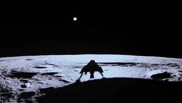
The LuGRE payload traveled to the moon aboard Blue Ghost Mission 1, a robotic lunar lander built by Firefly Aerospace under NASA’s CLPS program. CLPS, started in 2018, is a public-private partnership model through which NASA contracts commercial landers to deliver science and technology payloads to the lunar surface. Blue Ghost Mission 1 launched on Jan. 15, 2025, via a SpaceX Falcon 9 rocket and touched down on March 2, 2025. This made Firefly the first U.S. commercial company to successfully land on the moon upright, delivering 10 NASA-sponsored payloads, including LuGRE. The lander targeted a site near Mons Latreille in Mare Crisium, achieving a precision landing within ~100 m of the aim point. Built as a solar-powered lander about 2 m tall and 3.5 m wide, Blue Ghost was designed for a mission duration of one lunar day (~14 Earth days). By leveraging CLPS, NASA rapidly deployed LuGRE and other instruments, demonstrating the effectiveness of commercial partnerships in advancing lunar exploration. Blue Ghost’s successful landing and operations validated this approach and set the stage for upcoming CLPS missions in support of Artemis.
The LuGRE payload: Objectives and components
LuGRE is a technology demonstration aimed at determining whether Earth-originated GNSS signals can be reliably received and used for navigation at the moon’s distance. The payload was jointly developed by NASA and ASI with engineering by Qascom. Hardware on LuGRE includes a specialized weak-signal GNSS receiver, a high-gain L-band patch antenna array with RF filtering and a low-noise amplifier. This design allows it to track faint GPS and Galileo signals nearly 400,000 km from their transmitters. LuGRE specifically listens on multiple frequencies — GPS L1 and L5, and Galileo E1 and E5a — to maximize signal acquisition opportunities. The experiment’s objectives are threefold: (1) acquire and characterize GNSS signals in lunar orbit and on the surface, (2) demonstrate navigation fixes (position/time) using those signals at the moon, and (3) return data to inform the development of future lunar-specific GNSS receivers. All three of LuGRE’s objectives were met. During the mission, LuGRE began collecting and processing data en route to the moon (during a ~45-day transit) and also on the lunar surface after landing. As one of the first demonstrations of GNSS use on another world, LuGRE set out to prove that combined GPS/Galileo signals could enable autonomous navigation for spacecraft far beyond Earth.
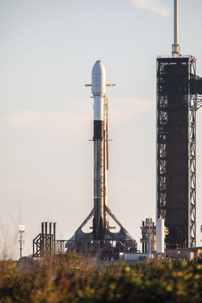
A SpaceX Falcon 9 rocket carrying Firefly Aerospace’s Blue Ghost Mission 1 lander prepares for a launch to the moon on Jan. 14, 2025, from Launch Complex 39A at the agency’s Kennedy Space Center in Florida. (Photo: NASA / Kim Shiflett)
Benefits of GNSS for lunar PNT
If proven reliable, GNSS-based navigation at the moon offers significant benefits for future lunar missions. First, it provides a common PNT framework for lunar explorers, akin to GPS on Earth, enabling precise real-time positioning and time synchronization for astronauts and robotic systems. This could allow lunar crews and rovers to navigate autonomously across the surface without constant ground support, reducing astronaut workload and dependence on Earth-based tracking. Accurate GNSS-derived position data improves safety and efficiency — for example, helping rovers avoid hazards and chart optimal routes or aiding astronauts in pinpointing resources, such as water, ice or scientific targets. Using existing GNSS signals also means that missions might rely less on cumbersome radio tracking from Earth or lunar beacons, simplifying mission operations.
In the long run, GNSS technology can support the development of lunar infrastructure: future base camps, power stations and landing pads could all reference a shared navigation grid, much as terrestrial infrastructure does. Additionally, leveraging well-known GPS/Galileo signals could reduce costs and technical risks, supplementing a proposed new lunar navigation satellite network.
LuGRE’s results have affirmed these possibilities. During transit, LuGRE broke records by tracking signals at 395,900 km out in lunar orbit, proving multi-constellation GNSS can aid navigation to and around the moon. Shortly after landing, it further demonstrated an autonomous GNSS navigation fix on the lunar surface, 362,100 km from Earth. These achievements suggest that even existing Earth-centric satnav can be extended to serve lunar exploration, a promising development for upcoming Artemis endeavors.
Challenges of GNSS reception on the moon
Adapting GNSS to the lunar environment is challenging. The main difficulty is the weakness of signals by the time they reach the moon. GNSS satellites orbit around 20,000 km from Earth, beaming most of their signal power toward Earth’s surface. At nearly 10 times that distance, only the spillover (side-lobe) signals reach the moon, arriving attenuated and sparse. This necessitates high-sensitivity receivers and high-gain antennas (such as LuGRE’s) to even detect the signals, along with sophisticated algorithms to pull meaningful data from the noise. The geometry and coverage also pose issues: a receiver on the moon will often see a limited number of GNSS satellites above its horizon, potentially affecting the accuracy and availability of navigation fixes. Local lunar conditions add further complications. The moon’s lack of atmosphere means no ionospheric delay, which is a positive for signal clarity. However, it also means that there is nothing to refract or scatter signals over the horizon — thus, terrain plays a crucial role. Rugged topography (mountains, crater rims) can block line-of-sight to GNSS satellites, and deep craters or polar shadowed regions might have very poor reception.
The pervasive lunar dust (regolith) can also be problematic because it may coat antenna surfaces or contribute electromagnetic noise, especially during landings or surface activities. These factors require advanced processing techniques and possibly integrating GNSS with other sensors to achieve reliable navigation. LuGRE’s design and operations were tailored to confront these challenges. For instance, using dual constellations doubles the pool of satellites and signals available, and collecting data both in orbit and on the surface helps characterize how signal quality changes in different lunar conditions. The knowledge gained will guide the development of next-generation lunar GNSS receivers with improved robustness against weak signals and intermittent coverage.
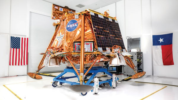
Firefly aerospace’s Blue Ghost Mission 1 lander is carrying 10 NASA science and technology instruments to the moon as part of NASA’s CLPS initiative and Artemis campaign. (Photo: Firefly Aerospace)
Implications for Artemis and deep space navigation
LuGRE’s success is a proof of concept that navigation aids from Earth can directly support moon missions. This is of immediate relevance to NASA’s Artemis program, which aims to return humans to the moon and establish a sustained presence there. Artemis crewed vehicles (such as the Orion spacecraft) and the planned Gateway lunar station could potentially use GNSS signals during transit or in lunar orbit to autonomously determine their trajectories. On the surface, future Artemis astronauts and rovers could carry GNSS-enabled devices to know their precise location without relying solely on Earth-based tracking. This capability will become increasingly important as activities expand — from pinpoint landing of resupply craft, to coordinating lunar base operations to enabling the first long-distance treks by crew or robots on the moon.
By proving GPS/Galileo usability at the moon, LuGRE also paves the way for establishing a standardized lunar reference frame tied to existing GNSS, which all international partners can use for joint operations. In a broader sense, LuGRE is a stepping-stone toward more advanced navigation systems in deep space. It demonstrates techniques (such as combining multiple GNSS constellations and using high-sensitivity receivers) that could inform navigation around Mars or other distant targets. While Earth’s GNSS signals won’t reach Mars with useful strength, the lessons learned can drive the design of Mars-orbiting navigation satellites or better onboard autonomous nav systems for deep-space probes. In essence, the experiment is accelerating the development of a GPS-like interplanetary navigation capability, crucial for humanity’s expansion deeper into the solar system.
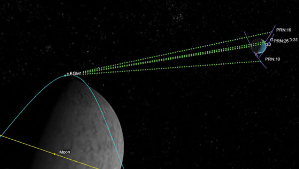
A Graphic representation of the relative geometry of Earth-moon-acquired GNSS satellites. (Photo: Agenzia Sapaziale Italiana)
Policy and international collaboration
The LuGRE mission exemplifies how international and commercial partnerships are shaping the future of space exploration. It was born out of a long-running collaboration between NASA’s Space Communications and Navigation program and ASI, reflecting a shared strategic interest in extending GNSS interoperability to the moon and beyond. The receiver hardware was developed by Qascom with academic support from Politecnico di Torino, underlining the role of industry and academia in innovation.
This NASA-ASI partnership built on earlier joint projects, such as GNSS receiver experiments on the ISS and suborbital flights, which tested using both GPS and Galileo for space navigation. Europe’s Galileo system, in particular, is a full partner in LuGRE. Its inclusion alongside GPS ensures that the experiment benefits from multi-constellation redundancy and also sends a message of GNSS interoperability, a key principle endorsed by the International Committee on GNSS. On the policy front, the mission aligns with U.S. space policy goals to develop services in cislunar space and encourages momentum in international standardization of lunar PNT frameworks.
Data from LuGRE will be made public, contributing to global research and possibly the drafting of new standards for lunar navigation that any nation’s spacecraft can adopt. The CLPS program itself, which enabled LuGRE’s delivery, represents a policy shift toward commercial sourcing of lunar services — fostering a market where companies such as Firefly, intuitive Machines, Astrobotic and others compete and cooperate to advance lunar science. As NASA leads the Artemis coalition with agencies from Europe, Asia and beyond, the LuGRE experiment offers a tangible product of cooperation: a foundation for shared navigation infrastructure at the moon. This collaborative, forward-looking approach will be critical as humanity returns to the moon not just to visit, but to stay.
Conclusion
LuGRE on Firefly’s Blue Ghost lander has marked a milestone in space exploration: it demonstrated for the first time that navigational signals conceived for Earth can be harnessed on the lunar surface. By uniting cutting-edge technical work (in receivers and antennas) with visionary policy support (via NASA’s CLPS and international GNSS cooperation), LuGRE showcases a path toward robust, autonomous navigation for the Artemis generation of missions. Achieving a GPS/Galileo fix on the moon is more than a symbolic first — it is a practical step toward a future where astronauts and robots navigate the moon — and one day Mars — with the same confidence as we do on Earth. The lessons from LuGRE will inform how we guide our spacecraft across the cislunar void, how we set up the positioning networks of tomorrow’s lunar bases and how nations cooperating can build the navigation backbone for a new era of deep-space exploration. In short, LuGRE has opened the door for GNSS to become an integral part of the lunar toolkit, blending technology and policy into a giant leap for navigation beyond Earth.
Since the dawn of GPS, researchers have worked to improve the accuracy of estimated positioning, navigation and timing (PNT) from the receiver-derived pseudorange, carrier-phase and Doppler measurements. While the pseudorange-based accuracy of standard point positioning (SPP) at the level of 1s to 10s of meters sufficed for most users, carrier-phase-based relative positioning, real-time kinematic (RTK), network RTK (NRTK) and precise point positioning (PPP) measurement processing techniques were developed to provide decimeter-to-centimeter-level PNT under various constraints. Of these approaches, PPP — generally based on the state-space reduction of measurement errors to a single GNSS receiver from a wide area calibration network — has evolved dramatically. Why should readers read this article, as PPP has been around for some two decades? Well, some communities may consider old performance specifications of conventional/classical PPP, a rather niche technology, for static use with post-processing of measurements, resulting in tens of minutes for solution convergence to the decimeter level. However, there have been many performance advances, with more coming, affecting who uses the technology and how.
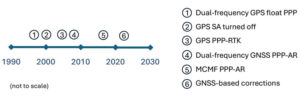
Figure 1: Timeline of PPP evolution.
Figure 1 illustrates the timeline of PPP evolution, from:
The development of the original technique in the late 1990s to reduce static GPS network measurement processing load.
The removal of GPS Selective Availability (SA), simplifying precise satellite clock prediction.
The development of PPP-RTK, in which regional RTK-derived corrections are used to reduce position convergence time and increase accuracy.
Successful isolation of PPP GPS dual-frequency carrier-phase ambiguities to increase accuracy.
Full multi-constellation, multi-frequency (MCMF) processing to greatly reduce position convergence time.
The introduction of GNSS constellation provider corrections. (Individual advances will be discussed in the Elements section.)
From initial scientific uses to becoming the commercial standard in remote areas or regions with limited GNSS terrestrial infrastructure, these research contributions are leading to ubiquitous open sky decimeter to centimeter-level positioning with a range of available corrections, increasing accuracy and reducing initial convergence for more applications.
Essentials
In the late 1990s, to improve positioning accuracy over SPP and avoid the heavy computational burden of network-adjusted relative positioning processing between many receivers, PPP algorithms (detailed in the Elements section) were formulated with undifferenced measurements between tracked satellites and a single receiver (Zumberge et al. 1997). Both pseudorange and carrier-phase measurements are utilized, with the former presenting many decimeter-level references and the latter ambiguous centimeter-level ranging. By filtering continuously tracked measurements over time, decimeter- to centimeter-level positioning is possible, as the state terms, including real-valued estimates of biased carrier-phase ambiguity terms — resulting in tens of minutes to hours of initial convergence time. This approach represents Hatch filtering in the position state rather than the observation domain. Key to PPP is the use of precise satellite orbit and clock estimates derived from a global reference network, which can receive measurements from an entire GNSS constellation. Additionally, to maximize performance, remaining error sources are modeled or estimated. While PPP was initially not as accurate as RTK and, more importantly, took tens of minutes to hours to attain solution convergence, the technique did not have the terrestrial infrastructure constraints of RTK or network RTK, which require reference receivers ~10 km to 15 km and ~75 km away, respectively. Once GPS Selective Availability was turned off in 2000, GPS satellite clock modeling became simpler and more accurate, and scientific and commercial PPP solutions quickly became the standard measurement processing technique for applications requiring decimeter-level accuracy in remote areas or places where it was not economically viable to install (an) RTK base station(s).
In the 2000s, two different approaches were developed to deal with the shortcomings of PPP: PPP-RTK and PPP-AR. In PPP-RTK, state space corrections from a regional NRTK solution are efficiently transmitted and applied as PPP corrections. As NRTK resolves carrier-phase ambiguities and estimates local atmospheric (ionospheric and tropospheric) refraction and reference station position all in a least-squares sense, PPP-RTK can produce centimeter-level positioning in seconds within a reference station network, where stations can be tens to hundreds of kilometers apart. In PPP-AR, the ionosphere-free linear combination of dual-frequency pseudorange and carrier-phase measurements is not employed; rather, the uncombined version, and the pseudorange and carrier-phase observation models, are extended to include and isolate satellite and receiver fractional carrier-phase biases, allowing PPP ambiguity resolution (AR) to integers with additional satellite code and phase biases from the network solution and between satellite single-differencing. Both approaches are having significant scientific and commercial success.
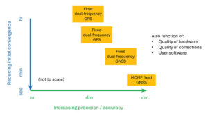
Figure 2: PPP and PPP-AR technology evolution in terms of accuracy versus convergence time.
Unlike RTK, which has the benefit of significant additional calibration information from the reference station, PPP(-AR) must rely only on satellite-based corrections and the strength of the single-receiver observations. In recent years, additional GNSS constellation satellites and frequencies have been brought on-line in large numbers, and GNSS constellation-provided PPP corrections have begun (Xu et al. 2021; Fernandez-Hernandez et al. 2022; Naciri et al. 2023). These developments have greatly increased estimation redundancy, making near-instantaneous PPP without regional reference stations possible (Naciri and Bisnath 2023). This evolution of PPP technology in terms of positional accuracy versus convergence time is illustrated in Figure 2. Therefore, it may be possible to a) dissolve the old GNSS duality of niche, professional-grade versus mass-market, low-cost hardware and software with low-cost hardware utilizing PPP (and RTK and PPP-RTK) software countermeasures to obtain precise PNT; and b) with PPP corrections from GNSS constellations, perhaps, as a reversion to SPP, to have PPP be the natural operational mode of precise GNSS PNT (Bisnath 2020).
Elements
Theoretical development
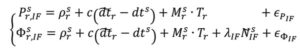
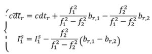
The PPP measurement processing technique utilizes the GNSS pseudorange (code) and carrier-phase (phase) observables. For receiver r and satellite s, the respective code and phase measurements on frequency can be defined as:
where and Φi : pseudorange and carrier-phase measurements, respectively, in meters; ρ: geometric range between receiver and satellite; c: vacuum speed of light; dtr and dts: receiver and satellite clock offset from GPS Time, respectively; γi = ƒ ⁄ ƒ : ratio of frequencies applied to first frequency ionospheric delay I to recover ionospheric delay at frequency i; Tr : zenith troposphere wet delay; M: mapping function to map to satellite-receiver line-of-sight troposphere delay; λi = c ⁄ƒi: signal’s wavelength; N : integer ambiguity on frequency i; br,i and b: receiver and satellite pseudorange hardware biases, respectively; Br,i and B : receiver and satellite phase biases, respectively; and рi and Φi : residual unmodeled errors such as multipath and noise in code and phase measurements, respectively.
where and Φi : pseudorange and carrier-phase measurements, respectively, in meters; ρ: geometric range between receiver and satellite; c: vacuum speed of light; dtr and dts: receiver and satellite clock offset from GPS Time, respectively; γi = ƒ ⁄ ƒ : ratio of frequencies applied to first frequency ionospheric delay I to recover ionospheric delay at frequency i; Tr : zenith troposphere wet delay; M: mapping function to map to satellite-receiver line-of-sight troposphere delay; λi = c ⁄ƒi: signal’s wavelength; N : integer ambiguity on frequency i; br,i and b: receiver and satellite pseudorange hardware biases, respectively; Br,i and B : receiver and satellite phase biases, respectively; and рi and Φi : residual unmodeled errors such as multipath and noise in code and phase measurements, respectively.
In order to eliminate ionospheric refraction, the original PPP solution forms the ionosphere-free (IF) linear combination of the dual-frequency GPS code and phase measurements:
From this combined form, the IF float PPP equations are (Kouba and Héroux 2001):
where the terms with tildes are biased by other terms from the starting observation equations, but allow for enough redundancy for user position, receiver clock offset, a zenith tropospheric term and real-valued, biased phase ambiguity terms to be estimated. In a sequential least-squares or Kalman filter optimal estimation process, positional accuracy depends on the quality of the satellite orbit and clock corrections, along with applying additional error modeling (including satellite and receiver antenna phase center offset and variation, solid Earth tides, ocean loading and phase wind-up), and, most importantly, the quantity, geometrical distribution and quality of the code and phase measurements. The state is initialized with m-level pseudorange measurements and slowly converges to the centimeter-level over tens of minutes to hours as the real-valued, biased phase ambiguity estimates reach steady state. This original or classic PPP solution, characterized by slow convergence to a fixed ambiguity-like positioning solution, may be what some in the community still think of as PPP.
PPP-RTK was developed as a means to remove these shortcomings of classical, float PPP by supplying PPP-like error state corrections from a regional RTK network to allow near-instantaneous carrier-phase ambiguity resolutionAR, (AR), solving both PPP’s convergence and accuracy problems (Wübbena et al. 2005). Significant operational improvements include increased spacing between (N)RTK reference stations, so less GNSS terrestrial infrastructure is required, and significant reduction in data transmissions from observation space representation (OSR) to state-space representation (SSR). By providing regional atmospheric corrections and ambiguity fixing, RTK-like performance is achieved but with larger CORS spacing. This approach has found commercial success in economically sustainable regions.
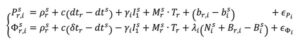
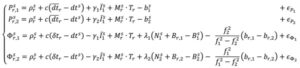
In parallel, active research continued in PPP-AR, given its desirable characteristic of not requiring regional reference stations. Multiple solutions were developed (e.g., Collins et al. 2008; Ge et al. 2008; Laurichesse et al. 2009), each of which reformulated the PPP observation equations to isolate the phase ambiguities, while overcoming datum defects in the estimation process. For example, the decoupled clock model (DCM) (Collins et al. 2008) isolates the phase ambiguities and directly estimates them as integers. The DCM does not make any assumptions regarding receiver biases and uses separate terms for code and phase clocks due to the imprecision in their synchronization — hence the model’s name. Satellite code and phase biases are required, along with satellite orbit and clock corrections. Then, standard AR methods, such as LAMBDA, can be applied. In the DCM, the fundamental code and phase equations are altered to:
where dtr, and δtr, are the receiver code and phase clocks, respectively. The receiver pseudorange bias br,i is parameterized in such a way that it is grouped into the receiver pseudorange clock forming dtr and ionospheric delay forming I . These terms are derived to be:
Through substitution, the DCM dual-frequency observation equations become:
In decoupling the receiver clocks, the carrier-phase measurements lose their datum. To remove the estimation singularities, one satellite is selected as the reference satellite, its ambiguities are fixed to arbitrary integer values and used for between-satellite single-differencing. N = N + δN , where N are the arbitrarily set integer ambiguities on frequency i and δ N are the differences between the actual integer ambiguities and the arbitrarily set ones. Carrier-phase cycle slips must be detected and changes to the reference satellite accounted for. While initial solution convergence is still a characteristic of uncombined, dual-frequency PPP-AR, the uncombined model solved the problem of brief data outages (solution re-convergence), as the slant ionosphere estimates are used as a bridging parameter between small data gaps.
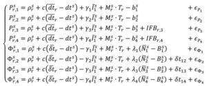
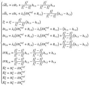
The dual-frequency model can be expanded to, e.g., quad-frequencies for multi-constellation, multi-frequency (MCMF) PPP-AR. Accounting for the use of a reference satellite per constellation, accounting for any spatial and temporal reference system differences between constellations, and additional inter-frequency pseudorange biases (IFBs) the up to quad-frequency DCM formulation can be derived as:
with:
There is therefore the need for accurate and consistent MCMF satellite orbit, clock, code bias and phase bias corrections. Some constellation-based corrections, e.g., from QZSS, BDS and Galileo, are appearing.
There is therefore the need for accurate and consistent MCMF satellite orbit, clock, code bias and phase bias corrections. Some constellation-based corrections, e.g., from QZSS, BDS and Galileo, are appearing.
Results and analysis
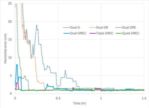
Figure 3: PPP-AR horizontal positioning error for various combinations of GNSS constellations and number of frequencies showing average initial convergence for IGS stations CUSV (Thailand), KIR8 (Sweden) and RABT (Morocco) on day of year 128 in 2024. Results presented are the average of 24 hours of data, reset every three hours.
How has PPP positioning solution convergence and accuracy evolved? The above model is now used to illustrate the performance of MCMF PPP-AR with up to four frequencies. The quad-frequency model has been implemented in the York-PPP client engine developed at York University. For performance illustration purposes, Centre national d’études spatiales (CNES) MCMF correction products are used for consistency and one day (day of year 128 in 2024) of high-quality MCMF GNSS observations are used from each International GNSS Service (IGS) stations CUSV in Bangkok, Thailand, KIR8 in Kiruna, Sweden, and RABT in Rabat, Morocco. Note that data from other days and other comparable stations produce similar positioning results. Simulated real-time, sequential least-squares, kinematic processing was performed for the following observation scenarios: 1) dual-frequency GPS (dual G); 2) dual-frequency GPS and GLONASS (float), with no ambiguity fixing of the frequency-division, multiple access GLONASS signals (dual GR); 3) dual-frequency GPS, GLONASS and Galileo (dual GRE); 4) dual-frequency GPS, GLONASS (float), Galileo and BeiDou (dual GREC); 5) up to triple-frequency GPS, dual-frequency GLONASS (float), triple-frequency Galileo and triple-frequency BeiDou (triple GREC); and 6) up to triple-frequency GPS, dual-frequency GLONASS (float), quadruple-frequency Galileo and quadruple-frequency BeiDou (quad GREC). Operational effects, such as correction latency, are not considered. Figure 3 demonstrates MCMF PPP-AR horizontal error initial solution convergence for these scenarios, averaged from each 24-hour dataset, reset every three hours across the three global stations.
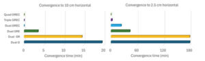
Figure 4: PPP-AR horizontal positioning convergence times for various combinations of GNSS constellations and number of frequencies to 10 cm and 2.5 cm for data used in Figure 3.
The dashed time series in figure show the benefits of adding constellations in the PPP-AR processing. From the average of the dual-frequency GPS solutions, the addition of each constellation reduces convergence time by approximately one-half. Then, by adding additional frequencies, convergence time is further reduced to basically instantaneous convergence using available measurements on up to four frequencies from all four GNSS constellations. These results bode well for GNSS data collection in sky-obstructed areas or with lower-quality hardware. Figure 4 provides the convergence times for the average solutions from each processing scenario to reach and sustain below 10 cm and 2.5 cm horizontal error, respectively. These are typical specifications for numerous static and kinematic applications. Four constellation, dual-frequency data are required to attain 10 cm horizontal positioning error or better near-instantaneously. However, to achieve the 2.5 cm convergence definition, at least triple-frequency data are necessary. The post-10 cm convergence horizontal solution accuracy, as defined by rms error, is 9 cm for dual-frequency GPS and 1 cm for each of the GREC processing scenarios. The post-2.5 cm convergence horizontal solution accuracy, as defined by rms error is 17 cm for dual-frequency GPS and 4 cm for each of the GREC processing scenarios.
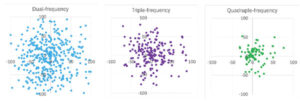
Figure 5: MCMF PPP-AR horizontal positioning error for dual-frequency GNSS (left), up to triple-frequency GNSS (center) and up to quadruple-frequency GNSS (right) for IGS stations CUSV (Thailand), KIR8 (Sweden) and RABT (Morocco) on day-of-year 128 in 2024. Results are epoch-by-epoch solutions in the north and east directions in centimeters with 8,640 position estimates in each scenario.
What if a more robust PPP solution is considered that also further analyzes the introduction of additional frequencies? The same three-station, one-day dataset can be processed in an epoch-by-epoch mode, where all filter states are reset. Therefore, there is no filtering with no assumptions about system dynamics. In this case, using a 30-second sampling rate, results in 8,640 position estimate “snapshots” — a robust process of estimation that can be useful for, e.g., clearly defining integrity for safety-of-life applications. The MCMF PPP-AR results for 1) dual-frequency GPS, GLONASS (float), Galileo and BeiDou (dual GREC); 2) up to triple-frequency GPS, dual-frequency GLONASS (float), triple-frequency Galileo and triple-frequency BeiDou (triple GREC); and 3) up to triple-frequency GPS, dual-frequency GLONASS (float), quadruple-frequency Galileo and quadruple-frequency BeiDou (quad GREC). Figure 5 illustrates the epoch-by-epoch horizontal positioning performance (in cm) for these three scenarios using planimetric subplots. Most position estimates for each scenario are near each subplot center. Adding measurements from the additional frequencies from the dual-frequency base to up to three frequencies and then up to four frequencies for the same four constellations greatly improves horizontal positioning precision and greatly reduces the quantity and magnitude of positioning outliers.
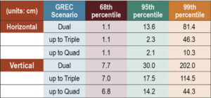
Table 1: MCMF PPP-AR positioning error for 68th, 95th and 99th percentiles (in cm) for data used in Figure 5.
Table 1 provides the epoch-by-epoch MCMF GNSS PPP-AR horizontal and vertical 68th (1-sigma), 95th (2-sigma) and 99th (3-sigma) percentile positioning error statistics for the same dataset. At the 68th percentile, all scenarios produce centimeter-level horizontal and sub-decimeter-level vertical positioning. However, at the 95th percentile, only triple- and quad-frequency processing can produce centimeter-level positioning in the horizontal component and near decimeter-level positioning in the vertical. To assess extreme position estimate outliers, the 99th percentile statistics show that dm-level horizontal positioning can be maintained with quad-frequency processing.
Table 2: Average estimation redundancy for data used in Figure 5.
The MCMF PPP-AR filtered results indicate that near-instantaneous, cm-level PPP is achievable with quality geodetic observations. The epoch-by-epoch, unfiltered results imply that robust, centimeter-level PNT is achievable. Table 2 provides the average redundancy in the epoch-by-epoch processing, where the redundancy is the difference between the number of measurements used and the estimation states. This measure provides insight to how the increase in the number of measurements, while not increasing the number of satellites or the dilution of precision, significantly improves PNT estimation performance for PPP-AR — as this is a measurement-driven technique. The average redundancy increases from 34 to 62 when expanding from dual-frequency GPS to dual-frequency GPS + Galileo and to 121 when using dual-frequency measurements from all constellations. Additionally, increasing processing to include up to triple-frequency measurements and quad-frequency measurements grows this metric to 154 and 183, respectively. The estimation process then becomes more robust against measurement errors and biases. It has more measurement strength to estimate all state parameters, including slant ionosphere refraction terms and integer ambiguities, allowing for improved position estimation precision.
Evolutionary
MCMF PPP-AR performance continues to improve. Positioning performance for quality geodetic measurements can produce horizontal centimeter-level positioning performance nearly instantaneously. Robust performance can be obtained with epoch-by-epoch processing, resulting in centimeter-level and few-centimeter-level horizontal and vertical positioning at the 95th percentile level using up to quadruple frequency measurements. Also, inclusion of additional measurements from additional frequencies greatly improves estimation redundancy, thereby improving state estimation.
Future research developments, testing and implementation include: adding measurements from available fifth frequencies; investigating less reliance on noisy and multipath-prone pseudorange measurements; expanding robust near-instantaneous PPP in urban environments; further defining/characterizing PPP integrity and safety integrity levels; having PPP be an independent or complimentary solution to/with (N)RTK for precise PNT; minimize requirements for atmospheric corrections; further use of PPP in mass-market hardware; and further integration of PPP as part of sensor suite solutions (e.g., automotive, smartphone, UAV, robotics, etc.) for resilient PNT.
Finally, what is the usefulness of the research in our lives? PPP measurement processing for GNSS is the scientific and industry standard for many user applications. There continues to be growing commercial adoption of this evolving technology, including expanded use in traditional (N)RTK precise applications, mass-market applications using low-cost hardware, and safety-of-life applications, including automotive, other passenger vessels, smartphones, robotics, UAVs and for aids to pedestrians.
EnSilica, a chip maker of mixed-signal application-specific integrated circuits (ASICs), has been awarded funding from the UK Space Agency under its Connectivity in Low-Earth Orbit (C-LEO) program. Following a competitive selection process, EnSilica has been awarded £10.38 million ($12.8 million) throughout the next three years for a development project pioneered by EnSilica.
“This is a great opportunity to accelerate our chipset development, enabling us to extend our portfolio of chips for the satellite broadband market with a focus on providing a complete solution for user terminals while reducing cost and power,“ said Paul Morris, EnSilica vice president of RF and communications business unit.
EnSilica provided its application with supporting letters of interest from potential lead customers to develop a family of semiconductor chips to support future generations of mass market satellite broadband user terminals. According to the company, the terminals will be capable of connecting with various satellite constellations and will leverage advanced semiconductor technology. In addition, the project will provide a resilient source of chips, which will be independent and not tied to specific satellite service operators.
The UK Space Agency’s C-LEO program was launched in 2024 and is designed to ensure that the UK space sector remains competitive in the rapidly evolving global market for low-earth orbit constellations. With a total funding pool of up to £160 million ($198 million) available over the next four years, the C-LEO program supports the development of smarter satellites, enhanced hardware, artificial intelligence-driven data delivery and improved inter-satellite connections.
This new project builds on EnSilica’s long history of collaboration with the UK Space Agency and the European Space Agency, alongside other key satellite communications partnerships and the company’s own investment in the technology.
Containers, stillages, trailers or reusable transport packaging — non-powered assets such as these play a central role in smooth supply chains and logistics processes. For a long time, however, non-powered assets could hardly be digitized due to a lack of sufficient battery life, thus eluding efficient management.
To plan and control logistical processes and supply chains, companies usually needed a large buffer/reserve stock and sometimes a lot of telephone/administrative work to determine the exact location and condition of such assets. Thanks to power-saving Internet of Things and wireless technology paired with high-performance sensors for environmental conditions and intelligent firmware, sufficiently robust trackers are now available for efficient use in the mass market.
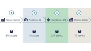
Figure 1: Integrated modeling tools help to model and track the flow of assets across operations and locations.
The basics: Thousands of tracker data at a glance
In order for companies to derive real benefits for their business from pure tracking, they need a management platform that can do more than display the trackers on a map. Depending on the requirements, tracking hardware can be equipped with sensors for temperature, humidity or tipping movements, for example.
A management platform must then ensure that the multitude of trackers can be efficiently commissioned and administered and that their collected data is made available for use. After all, large amounts of data are only valuable if important insights can be gained quickly and intuitively. The tracking application, therefore, needs powerful search and filter functions and visually meaningful maps, dashboards and panels.
Integration into existing systems
However, for the data collected via tracking to fully benefit the company’s supply chains and logistics processes, it needs to be integrated into the company’s existing IT systems, such as ERP systems or tools for data analysis and business intelligence.
The data exchanges between the business applications can be useful in both directions: on the one hand, precise localization and sensor data from the tracking platform enrich reliable enterprise resource planning via the ERP system; on the other hand, it can be helpful to make data from the ERP system available to the tracker management platform — for example, to evaluate the utilization of a trailer or to simply display the contents of a container via a mobile app on-site.
Technically, such data exchange can be realized through open APIs (application programming interfaces), which such a management platform should have. This enables the professional implementation of system integrations that are needed in the business IT of many companies — for example with SAP, Microsoft Azure or AWS.
Designing/modeling process flows and making route patterns transparent
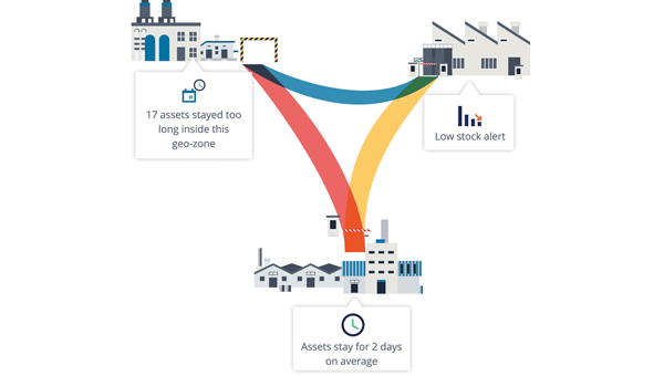
In order for companies to make their own processes around tracked assets transparent, a management platform needs tools that can be used to model and track the flow of assets across the different processes and, if applicable, locations (see Figure 1). Also important for this is the ability to define specific geographic areas of interest. Such geo-zones can then be used for inventory management, flow analysis or alerts. The mapping of load carriers or other assets to companies’ logistical processes and supply chains provides an accurate overview of how individual assets move from location to location, where they stop and for how long.
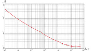
Based on the collected data, route patterns and travel times can be identified, rotation statistics with average and outlier analyses can be created (see Figure 2), and finally, planning and forecasts can be adjusted based on measured historical data. For appropriate visualization and evaluation, the tracking platform should provide the appropriate tools. This way, statistics can be generated for thousands of assets and/or an entire fleet, which can serve as a basis for further process optimization.
Figure 2: With a high-performance tracker management system, route patterns and travel times can be detected, and rotation statistics can be generated so that averages and anomalies can be identified.
Airbus example
Airbus develops, manufactures and delivers aerospace products, services and solutions worldwide, with more than 50,000 dedicated returnable transport packages circulating between sites and subcontractors. Thousands of returnable transport packages have been equipped with trackers and managed via a cloud-based platform over the past years. Airbus therefore benefits today from complete transparency. Inventory runs automatically, and stocks can be easily retrieved with their locations. The rotation capability of the packages has been improved, while their storage times and the circulating stocks have been reduced. Fleet capacity can also now be optimized, spare parts costs saved and subcontractor compliance better monitored.
The advantages at a glance
Precise inventory management of all mobile assets, from containers to returnable transport packaging to construction machinery.
Reliable condition monitoring: Continuous monitoring of environmental conditions such as temperature and humidity creates transparency — e.g., for compliance agreements.
Optimal process flows: Route patterns and turnaround times become transparent and anomalies easily identifiable, so that warnings can be sent in time and processes optimized overall.
Utilization monitoring: The utilization of each load carrier and each asset in a fleet can be precisely determined and optimized.
Predictive maintenance: Thanks to continuous monitoring, the maintenance of monitored assets can be planned and carried out in advance — before a breakdown interrupts important business processes.
Protection against theft: Lost or stolen assets can be easily recovered, so that financial damage can be minimized, especially in the case of expensive specialized assets.
The development and digital transformation of the global economy are based today on high-precision time synchronization of transport management processes, the transmission of electricity and data and many other processes. The high-precision global synchronization of GNSS spacecraft signals makes global instantaneous all-weather navigation possible and is the primary solution to the problem of time transmission.
For the past 57 years, since their adoption by the International Bureau of Weights and Measures (BIPM) as a unit of time measurement in the International System of Units of the Atomic Second, the technical characteristics of atomic frequency standards have increased significantly. The universally used Coordinated Universal Time (UTC) is based on the atomic time scale (AT), the readings of which are adjusted taking into account data regarding the Earth’s rotation.
Since its inception, GLONASS has relied on basic solutions embedded in the definition of UTC(SU). AT is formed by calculating the total number of vibrations at the resonant frequency of the energy transition between the levels of the hyperfine structure of the ground state of the cesium atom (133Cs) in the absence of external influences. It was based on this substance that the first ground and airborne frequency standards for GLONASS were created.
In accordance with the system’s interface control document, GLONASS transmits Moscow Time1, which is established by law by the Russian Federation. GLONASS transmits UTC(SU), which is formed as UTC+3 hours. In recent years, much work has been done to modernize the infrastructure for the formation of the national UTC(SU) time scale2. Today, the State Standard of Time and Frequency (SSTF) of the Russian Federation is one of the most modern time synchronization centers in the world. The basis of the SSTF are hydrogen frequency and time standards (HS) of the active type. The composition of the SSTF includes a storage complex of the national time scale based on the six newest active-type HS with a daily frequency instability of 3×10-16. In total, the SSTF consists of 18 HS.
Including new HSs in the composition of the SSTF has led to a significant increase in its contribution to forming the UTC scale. Currently, 87 time standards at national time laboratories contribute to the formation of UTC, which, following the recommendations of the BIPM time department, regularly provides measurement information of standards of the established format and content. In turn, the BIPM time division forms the International Atomic Time Scale (TAI) and the UTC scale. On a monthly basis, the BIPM Time Department publishes the results of the international key comparisons CCTF-K001.UTC and other data based on which a comparative analysis of the metrological characteristics of national standards is carried out.
The ALGOS algorithm is used for the formation of TAI and UTC2. It includes two main procedures: forecasting the drift of the frequency of standards and determining the contribution of specific standards to the final result — determining the statistical weight of standards.
Figure 1: Dynamics of the contribution of the world’s major time laboratories. (All figures provided by the authors)
Starting in September 2011, forecasting of the standards’ frequencies takes into account the frequency drift inherent in hydrogen frequency standards. The procedure for determining the statistical weight of standards was also changed; preference was given to the predictability of their frequency, which showed a more balanced distribution of statistical weights and increased the contribution of hydrogen standards to the formation of TAI and UTC.
Figure 1 shows the dynamics of the contribution of the world’s main time laboratories to the formation of UTC for 2022-2024: Russia – the Main Metrological Center of the SSFT, SU; United States – Naval Observatory, USNO; China – National Time Service, NTSC; Japan – National Institute of Information and Communication, NICT; France – Paris Observatory, OP; Sweden – Technical Research Institute, SP; Germany – Institute of Physics and Technology, PTB; Poland – Time Laboratory, PL. The WT contribution of each laboratory is calculated as the sum of the weights of all frequency standards, the measurement results of which this laboratory transmits to the BIPM. The weight of each individual atomic time and frequency standard is calculated monthly by the BIPM time division when calculating TAI and UTC based on an assessment of its frequency stability over the billing period.
The main characteristic of the HS, which affects the characteristics of the formation of time scales, is the instability of the frequency of the output signals. To quantify the frequency instability of the output signals, a number of characteristics are used that reflect both random and systematic frequency changes over time. The Allan variation has been widely used for more than 50 years as the main assessment of the frequency instability of the output signals of standards in the time domain.
At the same time, in terms of frequency instability, the SSTF atomic clock also occupies a leading position. In October 2022, the average weight of atomic clocks of laboratories in the formation of TAI and UTC increased significantly, from 1 to 1.2% to 1.4 to 1.6% (the best indicator for foreign laboratories is 0.5 to 0.7%). This indicator is calculated by dividing the total contribution of each laboratory by the number of its atomic clocks that participated in the formation of TAI and UTC in the period under review. The average contribution more correctly characterizes the quality of the frequency standards of each time laboratory.
Additionally, an important indicator is the percentage of atomic laboratory clocks having the maximum allowable BIPM weight for an individual frequency standard. For 2022-2024, the figure ranged from 80% to 100%. The maximum possible weight depends on the total number of frequency standards involved in the formation of UTC in a particular billing period. This indicator was calculated as the number of atomic clocks having the maximum permissible weight divided by the total number of hours of this laboratory in each calculation period. All HSs from the SSFT have the highest rates of frequency instability and for most of the period under review make the maximum possible contribution to the formation of TAI and UTC.
Figure 2: Comparative estimates of national time scale shifts. (All figures provided by the authors)
The characteristics of the Russian HS directly impact the formation of the national atomic and coordinated time scales of the Russian Federation TA(SU) and UTC(SU). Figure 2 shows the differences between national time scales and UTC.
Coordinated Universal Time(k) relative to UTC in 2022-2024.
The analysis of this data allows us to conclude that the UTC(SU) national coordinated time scale is one of the best national implementations of UTC, and the national atomic time scale TA(SU) occupies a leading position in terms of instability among the scales implemented in the leading national time laboratories.
GLONASS’ time scale is linked to the readings of the SSTF, taking into account the correction of the Moscow decree time and are implemented by the GLONASS synchronization system, which is also based on hydrogen frequency standards. Figure 3 shows the discrepancy between the values of the GLONASS system time relative to the UTC(SU) time, which is currently less than 10 ns.
Figure 3: Error in transmitting the national time scale of the Russian Federation UTC(SU) using GLONASS. (All figures provided by the authors)
UTC(SU) parameters are transmitted via GLONASS spacecraft and the first of the fourth-generation spacecraft, which has a passive hydrogen maser (PHM) on board, was launched into operational orbit on Aug. 7, 2023. In the spring of this year, flight tests of this device began, which showed an improvement in the accuracy of time transmission during the transition from the cesium to the hydrogen standard.
Figure 4: The discrepancy between the spacecraft time scale and the UTC scale: 1 – Glonass-K2, orbit slot 26, 2 – Glonass-M, orbit slot 12. (All figures provided by the authors)
Figure 4 shows the magnitude of the discrepancy between the time scales of the two GLONASS spacecraft. The cesium frequency standard installed on board the Glonass-M shows some of the best characteristics in the entire 20-year history of these spacecraft and demonstrates a daily relative frequency instability of 2×10-14, which is five times better than the design characteristics. Preliminary results of the use of the PHM as a source of reference vibrations and time synchronization pulses on board the Glonass-K2 in the same time interval shows a decrease of more than two times in the fluctuation error of forecasting the time scale with a relative daily instability of 7 × 10-15.
Similar characteristics emerge when using the most conservative spacecraft control scenario. Here, the update of the on-board clocks parameters (OCP) of the on-board time scale departure model relative to the system is carried out once per turn, i.e. once every 11 hours and 45 minutes. This ensures a decrease in the value of the OCP contribution to the error of navigation definitions due to the space complex before updating them from 1.4 m with a daily instability of 1×10-13 to 0.1 m for a relative daily instability of 7×10-15. The results obtained make it possible to redefine the basic onboard standard and switch to the priority use of the HPM signal for the formation of reference oscillations and clock synchronization of GLONASS spacecraft signals.
Figure 5 Passive hydrogen maser VC-1017. (All figures provided by the authors)
Further development of this technology provides for installing a VC-1017 small frequency standard on board (Figure 5). Compared with the one presented in a previous article, this standard is more than two times lighter while maintaining the stability characteristics of the formation of reference vibrations (Figure 6).
Figure 6 Measured instability of the VCH-1017 frequency relative to the state primary standard of time units, frequency and Russia’s national time scale for 40 days. The frequency drift was 1.51×10⁻¹⁵. The daily instability with the exception of drift is 1.42×1. (All figures provided by the authors)
The launch of the Glonass-K2 spacecraft with the prototype of this HPM is planned for the first half of 2025. Its precision characteristics allow us to expect a further increase in the stability of time transmission by GLONASS.
A significant improvement in the metrological characteristics of hydrogen frequency standards is achieved using a new system for forming a beam of atoms in a single energy state, which was developed before their industrial use. Thus, the daily frequency instability in active hydrogen frequency standards using a new beam formation system reached the level of (6-8) ×10-17.
Figure 7: Microwave resonators for passive hydrogen frequency standards. (All figures provided by the authors)
The basis for creating passive frequency standards of various sizes was the pioneering invention of an oscillatory structure, which is used in all passive hydrogen frequency standards for global navigation satellite systems. This microwave resonator made it possible to change the dimensions at a constant resonant frequency of 1,420,405,751 Hz, close to the frequency of the atomic transition. At the same time, the design proved to be suitable for harsh operating conditions, including requirements for the launch of the spacecraft. (Figures 7 and 8).
Figure 8: Microwave resonators of different sizes for passive hydrogen frequency standards. (All figures provided by the authors)
Reducing the size of the “heart” of the frequency standard allows you to reduce the weight of all other structural elements — thermostats, magnetic screens, vacuum caps, supports, etc. At the same time, it is easier to achieve structural rigidity requirements and reduce the influence of destabilizing factors.
The most important factor influencing the metrological characteristics of passive hydrogen frequency standards is the automatic frequency tuning system of the quartz oscillator to the frequency of the spectral line.
Careful engineering of the auto-tuning system avoids the influence of control circuits on each other. In addition, a technical solution has been introduced in the new frequency standards of the GLONASS system, which makes it possible to reduce the impact of various factors on the stability of the output frequency.
The results obtained allow us to consider the coming year 2025 as an important milestone in the development of time transmission technologies through the GLONASS system.
The HSRP is a federal advisory committee that provides NOAA with independent advice on improving the quality, efficiency, and usefulness of NOAA’s navigation-related products, data, and services. The HSRP advises the NOAA Administrator about its navigation (i.e. nautical charts and ENCs), physical oceanographic (i.e. tides & water levels), geospatial, positioning, and coastal and shoreline programs, products, and services. There are two public meetings each year in different port regions at which public comments from stakeholders and partners are sought. Most of the meetings include webinar capability for those not in the area.
See an excerpt below of the agenda for the three-day meeting. These meetings are open to the public and I would encourage anyone interested in the activities of these program offices to participate in the meetings. Participants can attend in person or virtually via webinar. I participated in the meeting in virtual mode. The HSRP website provides links to reference documents, presentations, and recordings.
This newsletter will highlight the session on the NGS Geospatial Modeling grants.
Excerpt from the HSRP 2024 Fall Meeting Agenda
September 24, 2024
Presentations:
Opening and welcome
Mr. Sean M. Duffy, Sr
Mr. Mark Schrupp
Sen. Peters (MI), video
Rep. Theander (MI), video
Ms. Rachael Dempsey
RDML Benjamin Evans
Opportunities and Challenges for the NOS’s Navigation Observations and Positioning Portfolio
Moderator: Ms. Rachael Dempsey
Dr. Larry Mayer
Dr. Marian Westley
RDML Benjamin Evans
Dr. Shachak Pe’eri
Directors FSK update
Local, Regional, State Stakeholder and Partner Perspectives on NOAA Navigation Services
Moderator: Mr. Eric Peace
Capt. Richard Armstrong
Mr. Paul LaMarre
Capt. Tony Brandano
Capt. Peter Barry
Mr. Derek Cusimano
Underserved Communities Mapping and Charting needs in the Great Lakes Region
Moderator: Mr. Nathan Wardwell
Dr. Jennifer Boehme
Ms. Stephanie Gandulla
Mr. Ed Bailey
September 25, 2024
Vdatum
Dr. Shachak Pe’eri
International Great Lakes Datum (IGLD)
Dr. Jacob Heck
Ms. Sierra Davis
HSRP Working group:
HSRP Technical Working Group Report
September 26, 2024
NGS Geospatial Modeling Grants
Moderator: Mr. Galen Scott
Dr. Jeff Freymueller (Ph.D.)
Ms. Mara Figueroa Berrocá
Great Lakes Perspectives on National Drivers
Moderators: Mr. Nathan Wardwell and Mr. Eric Peace
Ms. Erika Jensen
Mr. John Bratton
Mr. Mark Breederland
Mr. Ryan Chatland
NOAA Center of Excellence for Operational Ocean and Great Lakes Mapping
The session on NGS geospatial modeling grants provided updates by representatives from MSU (Jeff Freymueller) and OSU (Mara Figueroa Berroca). I have provided a few highlights below, but I encourage everyone to download the presentations and/or listen to the daily recording.
Freymueller highlighted that keeping the error in coordinates small in a spatial reference system is hard to do in a deforming Earth. This is very important to all users of the National Spatial Reference System (NSRS). Not all CORS are created equal, and their coordinates can change based on various factors such as earthquakes, equipment changes, and local deformation due to the extraction of groundwater. Therefore, efficiently and effectively monitoring the CORS is necessary to quickly identify issues and correct coordinate values in a timely manner. MSU developed a CORS Dashboard that provides a tool for monitoring CORSs. Freymueller provided a slide depicting an example of a CORS in California. See the image below.
MSU CORS dashboard. (Photo: HSRP Website)
Plots of GLO2. (Photo: HSRP Website)
That said, Freymueller stated that crustal deformation and changes in CORS coordinates is not just a California issue. He provided a slide of a plot of a station in Wisconsin (see the image below.) The plot highlights changes in values where there’s an undocumented offset, a change in antenna, and an elastic deformation due to a change in water load in the Great Lakes.
Plot of ABMS. (Photo: HSRP Website)
As previously mentioned, keeping the error in coordinates small in a spatial reference system is hard to do in a deforming Earth, especially when so many factors affect coordinates, such as the changing load of water on the Great Lakes. The MSU CORS Dashboard will provide a tool for monitoring the CORS and identifying issues associated with coordinates of the CORSs.
The MSU CORS Dashboard plans include having different modules for various purposes:
Compare Solutions:
With other solutions
With Velocity Model
Compute and Display Metrics and select CORS stations based on metrics.
Earthquake and Postseismic Deformation Modeler:
Ingest fault model solutions and generate predictions
Statistics on agreement of different fault models
How well do the range of geophysical models agree?
Forward predict postseismic deformation
The MSU CORS Dashboard provides information about CORSs that could be useful to surveyors and mappers when performing and analyzing a GNSS survey project. For example, one module will compute and display metrics about individual CORSs, providing surveyors with the appropriate information to select the best CORSs for their GNSS project. NGS and MSU will determine how this CORS Dashboard is incorporated into NGS products and services.
Another phase of the MSU geospatial modeling grant included developing a geodesy program to help address the U.S. geodesy crisis. The presentation provided several slides with information on students obtaining a master’s degree in geodesy. The coursework for the two-year online program is divided into four thematic areas: Foundations of Geodesy, Fundamentals of Geodesy and Geophysics, Mathematical and Computational Concepts, and Geodetic Methods and Applications. Students will take a mix of courses (no thesis) from the consortium institutes – MSU, Michigan Technological University (MTU and the University of Alaska Fairbanks (UAF).
The following is a Timeline for Development:
2024: Develop University consortium agreements and establish structure for master’s program
2024/2025: Develop courses
Fall 2025: Launch program with first class of students
Freymueller mentioned that the timeline for launch currently feels optimistic due to bureaucratic hurdles dealing with the consortium agreements, but they are continuing work on the development of courses. Further newsletters will provide updates on the progress of the program.
Outline of Geodesy Master’ Degree
Foundations of Geodesy
Courses:
Map Projections (MSU)
Geodetic Models (MTU)
Both courses required
Courses provide backgrounds in mapping, projections, datums, reference frames, and transformations.
Fundamentals of Geodesy and Geophysics
Courses:
Modern Geodesy and Applications (MSU) or Geodetic Methods and Applications (UAF)
Geodetic Data Processing and Analysis (MSU)
Solid Earth Geophysics and Geodynamics (MSU) or Foundations of Geophysics (UAF)
Positioning with GNSS (MTU)
Students choose at least 2 courses
Courses provide background in geodetic theory (including orbit determination and GNSS and imaging satellite systems), measurement and interpretation of steady state and time variable motions within the solid Earth, cryosphere, and hydrosphere, data processing, and geophysical modeling.
Mathematical and Computational Concepts
Courses:
Introduction to Numerical Tools for Earth and Environmental Sciences (MSU)
Programming and Automation for Geoscientists (UAF)
Data Analysis and Adjustments (MTU)
Inverse Problems and Parameter Estimation (UAF)
Numerical Analysis (UAF)
Students choose at least 2 courses
Courses will provide foundation in programming and mathematical techniques (including inversion theory and linear regression) essential for geodesy
Geodetic Methods and Applications
Courses:
3D Surveying and Modeling with Laser Scanning Data (MTU)
Courses extend knowledge into additional land- and satellite geodetic techniques, network design, and geophysical applications
The second presentation on the geospatial modeling grants was titled “Developing a Fully Kinematic, Backwards-Compatible Reference Frame for the Continental United States of America and Canada,” presented by Mara A. Figeroa, OSU.
OSU Presentation. (Photo: HSRP Website)
Figeroa outlined the following project goals:
Development of the operational (sandbox) kinematic reference frame (KRF).
Develop automation processes to detect and model deformation resulting from earthquakes, GIA and other crustal motions.
Parallelization wrapper for M-PAGES (adapted from our existing Parallel.GAMIT)
Process all existing data in the U.S. and Canada
Creation of Intraframe deformation models (i.e. trajectory prediction models)
Use GNSS and InSAR aided by AI to access the conventional epoch of the frame.
Provide the users with maps of “stable areas” to facilitate access to the frame using differential processing.
Figeroa noted that the coordinates and model parameters defining the reference frame are time-dependent in a National-Level Kinematic Reference Frame (KFR). The KFR needs to provide multiple conventional epochs that are accessible to all users anytime and anywhere to guarantee topologic homogeneity. Models need to be updated to account for the changes in coordination due to earthquakes and other deformation events. Figeroa stated, “Kinematic implies constant update of the reference frame parameters to ‘honor’ the frame’s internal geometry.”
OSU has developed what they denote as a Geometric Geodesy Processing Line (GGPL) to evaluate and analyze CORSs data. They are processing all CORSs data to identify issues with the data that could be due to various factors such as crustal deformation and equipment changes. The tool highlights stations with a potential warning flag issue (see OSU Interactive GGPL).
OSU Interactive GGPL. (Photo: HSRP Website)
The system is automated, but they have developed interactive visual tools so researchers can review the results of each station. The visual interactive GGPL provides metadata about the station such as coordinates, maps, photos, and dates of installation of equipment.
OSU Interactive GGPL – Location and Photo. (Photo: HSRP Website)
OSU Interactive GGPL – Equipment. (Photo: HSRP Website)
OSU Interactive GGPL – Coordinates and Other Metadata. (Photo: HSRP Website)
One feature of the GGPL is that it generates plot changes in coordinates over time (see the image below). I recently participated in a School of Earth Science Advisory board meeting at OSU and visited with Demian Gomez, Ph.D., the project’s lead principal investigator.
Demian demonstrated the GGPL tool for me. I was really impressed at how fast the system was, as well as how much information it provided in a user-friendly format. In my June 2024 GPS World Survey Scene newsletter, I highlighted an issue I found with an antenna change at a CORS in Texas. I ask Demian to pull up the information for the same site. The GGPL highlighted the same antenna change and shift in coordinates that I found. This feature is important to developing an intraframe deformation model (IFDM). How NGS will use this in the development of the IFDM2022 for the new, modernized NSRS will be determined later by NGS.
An important aspect of an IFDM is to identify and model changes in coordinates due to crustal deformation. As mentioned by Freymueller, modeling earthquake and other deformation events is extremely important to maintaining an accurate spatial reference frame. OSU GGPL tool assists in identifying potential deformation due to earthquakes.
OSU Interactive GGPL – Detection of Earthquakes. (Photo: HSRP Website)
OSU’s process includes developing trajectory prediction models (TPM). Trajectory prediction models need to be continuous in space and time to predict the behavior of passive benchmarks. Accurate trajectory prediction models will ensure access to a geodetic reference frame after big earthquakes utilizing accurate post-seismic coordinates. OSU’s process includes developing techniques for observing GNSS networks in sparse areas to improve the model’s predictability. My May 2024 GPS World Survey Scene newsletter highlighted Demián’s extensive experience modeling time-dependent coordinates and several papers published in the Journal of Geodesy addressing this topic. The papers have demonstrated the model’s effectiveness in earthquakes in Argentina and have developed tools that provide coordinates in updated reference frames based on the models. This is important to users of the new, modernized NSRS because the accuracy of the IFDM2022 model is vital to providing accurate Reference Epoch Coordinates (RECs) in the new, modernized NSRS. See my August 2022 GPS World Survey Scene Newsletter for information on RECs and my May 2024 GPS Newsletter for more details on Demián’s work.
Model of Co-seismic Component. (Photo: HSRP Website)
This newsletter highlighted the progress that OSU and Michigan State University have made in developing tools that will be useful for developing and implementing the new, modernized NSRS in 2025.
As I previously mentioned, I would encourage everyone to download the presentations and recordings for more details. The recording of the session on NGS Geospatial Grants can be found on the Sept. 26, 2024, recording. (The session on NGS Geospatial Grants starts at 1:02:45 on the recording.)
Similarly to my previous newsletter, I want to remind everyone that in less than a year, NGS will finalize the new terrestrial reference frames and geopotential datum. Time really is running out and users need to obtain a working knowledge of the new, modernized National Spatial Reference System.