Author: Richard B. Langley

Innovation: One Year in Orbit
GIOVE-B E1 CBOC Signal Quality Assessment

By Matthias Söllner, Christian Kurzhals, Wolfgang Kogler, Stefan Erker, Steffen Thölert , Michael Meurer, Maktar Malik, and Manuela Rapisarda

GIOVE-B has been in orbit for just over one year. How well is it performing? In particular, what can we say about one of GIOVE-B’s pioneering features: its E1 CBOC signal? In this month’s column, we take a detailed look at a particular monitoring and assessment program set up to examine the GIOVE-B signals and discuss some of its initial CBOC results. The successful operation of this program bodes well for its use in future validation campaigns.

INNOVATION INSIGHTS by Richard Langley

THE SECOND GALILEO TEST SATELLITE, GIOVE-B, was launched on April 27, 2008, and began transmitting navigation signals a few days later. It joined its older sibling, GIOVE-A, which was placed in orbit over two years earlier. Standing for Galileo In-Orbit Validation Element, the GIOVE satellites constitute the first in-orbit test phase in the development of the Galileo navigation system.

In addition to securing the frequencies for the system, the satellites are being used to assess key technologies for the full Galileo constellation. The GIOVE test phase will be followed by the In-Orbit Validation (IOV) phase during which four IOV satellites will be launched, two at a time, aboard Soyuz rockets from Europe’s spaceport in French Guiana. Together with a preliminary ground network, the IOV satellites will be used to validate the Galileo system as a whole, using advanced system simulators. The launches are expected to occur by the end of 2010.

But before the IOV phase can begin, a thorough analysis of the performance of the GIOVE satellites must be carried out to minimize any difficulties with the IOV satellites. This includes monitoring and assessing the different signals broadcast by the satellites.

The GIOVE satellites can transmit on all three Galileo frequencies, E5, E6, and E1 (also known as L1) but only on two simultaneously (either E1-E5 or E1-E6). A variety of modulation types can be transmitted on the different frequencies by both satellites to test their use for the different Galileo services to be implemented for the operational constellation. These include alternative binary offset carrier (BOC) and quadrature phase shift keying on E5 and cosine BOC (BOCc) and binary phase shift keying on E6. On E1, the satellites have different capabilities. Although both satellites can transmit BOCc on this frequency, GIOVE-A can additionally transmit a single BOC signal with a subcarrier frequency of 1.023 MHz and a spreading code chipping rate of 1.023 MHz (BOC(1,1) ) whereas GIOVE-B transmits a more versatile multiplexed composite BOC or CBOC, which linearly combines BOC(1,1) and BOC(6,1). The CBOC signal is being transmitted by GIOVE-B to explore its performance, usability, and any possible side effects including its use in receivers designed to track a BOC(1,1) signal.

GIOVE-B has now been in orbit for just over one year. How well is it performing? In particular, what can we say about one of GIOVE-B’s pioneering features: its E1 CBOC signal? In this month’s column, we take a detailed look at a particular monitoring and assessment program set up to examine the GIOVE-B signals and discuss some of its initial CBOC results. The successful operation of this program bodes well for its use in future validation campaigns.

The first measurements of the navigation signals transmitted by the second Galileo test satellite, GIOVE-B, were recorded during the night of May 7, 2008, following the successful launch from Baikonur a little over a week earlier on April 28. During the In-Orbit Test (IOT) phase of the mission, which lasted about three months, a program of intensive measurements was carried out by the German Aerospace Center (Deutsches Zentrum für Luft- und Raumfahrt or DLR) and the Astrium subsidiary of the European Aeronautic Defence and Space Company (EADS) using the 30-meter high-gain antenna at Weilheim/Lichtenau, near Munich, Germany. These and follow-on activities were performed under a bilateral agreement between the European Space Agency (ESA) and DLR’s Institute of Communication and Navigation on the exploitation of the GIOVE satellites.

The first measurements indicated that the navigation payload suffered no damage or degradation with regard to power and signal-in-space (SIS) quality during the launch of the satellite. After the successful completion of the IOT phase, the satellite configuration was maintained for long intervals to allow stability and long-term quality assessments within the ESA GIOVE mission activities and to stabilize ground segment operation. DLR and Astrium continued their measurements and analysis on GIOVE-B signals, focusing on modulated power and on modulation and correlation quality. The observation intervals included an eclipse season, when GIOVE-B spends a fraction of its orbit in the Earth’s shadow. Any impact of the corresponding temperature variations on signal transmission characteristics and key navigation parameters was of special interest.

This article focuses on modulated spectral power analysis of GIOVE-B signals for the detection of frequency and elevation-angle-dependent variations in the transmitted signal spectrum and power. Also, a detailed in-phase/quadrature-phase (I/Q) sample analysis is presented, focusing on modulation correctness and correlation distortions. These assessments are based on sample files of a few seconds of navigation signals as received by a calibrated high-gain antenna and recorded with the BayNavTech Signal Experimentation Facility (BaySEF). We have evaluated, in particular, correlation loss and S-curve bias since these parameters are very sensitive to onboard signal distortions although their reliable evaluation is quite challenging. In this article, we concentrate on the analyses of the E1 composite binary offset carrier (CBOC) modulation.

We discuss the GIOVE-B measurement and evaluation parameter results from the initial IOT phase and from later phases, including those from an eclipse period. This comparison of measurement results — spread over the first year of operations — demonstrates the excellent stability of signal power, modulation, and correlation quality of the GIOVE-B signals.

GIOVE-B E1 Signal
GIOVE-B can transmit navigation signals either simultaneously in the Galileo E5 and E1 bands or in the E6 and E1 bands. At E1, with a center frequency of 1575.42 MHz, GIOVE-B transmits three signal components called E1-A, E1-B, and E1-C. The E1-A signal has a BOCcos(15,2.5) modulation, with 2.5575 MHz code chip-rate and a binary cosine-type subcarrier modulation of 15.345 MHz. The B- and C-components have CBOC(1,6,1,10/1) modulation. Within this type of multiplexed BOC implementation, the code chips are provided at a constant rate of 1.023 MHz, modulated with a composite quaternary subcarrier with rates of 1.023 and 6.138 MHz. The latter part, called the BOC(6,1) subcarrier, has a relative power of 1/11 and is added to the BOC(1,1) binary subcarrier in CBOC-B and subtracted for CBOC-C. From the beginning of May 2008 until July 2009, GIOVE-B transmitted signals 96.8% of the time. Considering the experimental nature of the satellite, this represents a very successful operation.

Signal Quality and Relevance
In GNSS operations, signal quality assessment generally refers to the behavior of the navigation signals as transmitted from individual satellites. In this article, we assess two major aspects: the transmitted signal power and the frequency-transfer distortions of the satellite relative to the ideal signal definitions.
Why should we consider these aspects in particular? For transmitted signal power, the answer is obvious. In addition to proof of compliance with regulatory declarations, verification and monitoring of signal power is relevant for the system provider to commit to certain navigation service performance.

Concerning frequency-transfer distortions, the answer may be less obvious. The relevance is obtained via the impact of distortions on a receiver’s correlation function. First, the available maximum correlation power for a receiver binary replica may be affected. This is due to changes in the power sharing of the signal components within the complete signal and due to reduced matching of distorted transmitted signals with the ideal receiver replica. Second, the shape of the correlation function may suffer from asymmetric distortions, leading to receiver-dependent biases in the discriminator lock point. The most relevant receiver parameters are the input bandwidth and the discriminator type, especially the discriminator spacing (early-late spacing). With respect to this, user receivers and receivers in the control system ground segment (used to derive the satellite orbit and clock parameters) may differ. This leads not only to timing but also to positioning errors, if the distortions are different for different satellites.

These are the main reasons why we need to analyze and control the corresponding distortions for the Galileo system.

For an accurate assessment of transmitted signal power and frequency distortions, we had to obtain measurements with a highly directive antenna. This is essential in order to lift the instantaneous signal far above the noise floor and to avoid environmental distortions from interference as well as multipath.

But why don’t we consider also other aspects of signal quality such as the correctness of the navigation message or the stability of hardware delays and clocks? Because measurements with the highly directive antenna are not so appropriate for an assessment of these parameters. Instead, continuous monitoring over weeks or longer is preferred, based on measurements from a network of distributed navigation receivers. Such monitoring likely will be discussed in other publications.

Figure 1: Illustration of S-curve bias parameter.

Evaluation Parameters
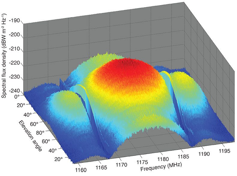
For the assessment of the satellite’s radiated power in the individual navigation bands, absolute calibrated spectral measurements are evaluated for spectral flux densities integrated over frequency. These parameters provide a first insight into spectral asymmetries and variations over time.

Other parameters are used to evaluate the distortions in the instantaneous transfer characteristics of the satellite. They are derived from wide-band recorded baseband-signal samples of up to a few seconds duration.

Initially, we consider the I/Q probability density of the signal after Doppler frequency shift removal, well known from communication system analysis as scatter plots. Secondly, as introduced in the previous section, we want to quantify the impact of transfer distortions on the navigation performance obtained for ideal navigation receivers. The corresponding acquisition and tracking performance is based on the correlation function.

We define the normalized correlation function with respect to ideal receiver properties in order to separate the satellite transmit distortions of interest from receiver distortions according to the following equation:

with
- the preprocessed baseband signal, SBB-PreProc, with down-converted nominal center frequency, full Doppler removal, and brick-wall-filtered to a bandwidth of interest;
- the reference-signal, SRef, providing the ideal binary (or, for CBOC, quaternary) baseband receiver replica signal;
- the integration period, Tp, often corresponding to the primary code period of the reference signal under consideration.
From this normalized correlation function, we can derive the primary relevant navigation parameters, which are, as previously mentioned:
- correlation loss
- early-late spacing dependency of the code-loop-discriminator lock point and S-curve bias.
Figure 2: GIOVE-B E1 CBOC measured and ideal normalized power spectral density.

Correlation Loss. For a given (distorted) signal, the correlation loss (CL) quantifies the loss in correlator output power relative to an ideal signal. This can be formulated by

where

It should be noted that the ideal baseband signal here is the multiplexed signal including all signal components, also band limited with a brick-wall filter to the bandwidth of interest.

S-Curve Bias. The navigation receiver obtains the (noiseless) code delay by following the zero crossing of the code discriminator. The output as a function of delay resembles the letter “S” or its reflection and is called the S-curve. For asymmetric distortions in the correlation function, it turns out that different code-tracking loops may have different lock points, as illustrated in FIGURE 1 for an arbitrary example.

To quantify this effect with a reasonable compromise between parameter complexity and practical value, a non-coherent (early minus late) power discriminator is considered over a wide range of early-late spacings, . This refers to the code discriminator of

with its lock point, , defined by

.

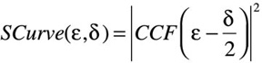
Then, the spreading of the lock point is the S-curve bias, SCB, given by

,

considering all δ in the range [0, δ_max], with

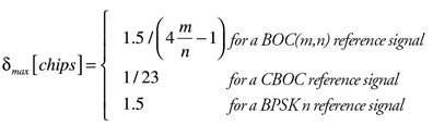
Those interested in additional candidate signal-quality parameters, more detailed descriptions, or a theoretical analysis of the impact of satellite distortions on navigation performance parameters should consult the paper “GNSS Offline Signal Quality Assessment” listed in Further Reading.

Figure 3: GIOVE-B E1 CBOC received power flux on May 11, 2008

Weilheim Measurement Setup

As previously mentioned, for accurate measurements of the various signal-quality parameters, the signal needs to be lifted above the noise and multipath, and any interference needs to be suppressed considerably. Moreover, as the signal quality from the satellite needs to be assessed separately, any measurement-system transfer distortions need to be calibrated out as much as possible.

That’s why DLR installed a measurement and calibration system at their 30-meter high-gain dish antenna at Weilheim for GIOVE signal performance measurements. This measurement setup was completed for high capacity signal recording with one rack of the BaySEF equipment in cooperation with EADS Astrium.

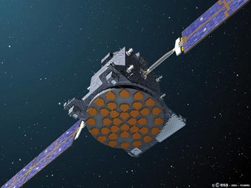
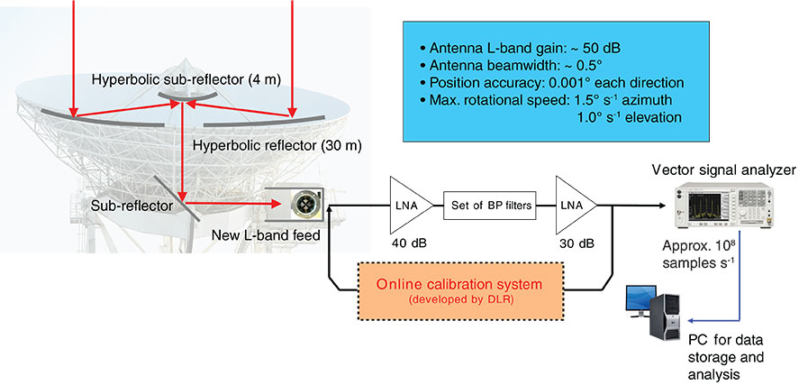
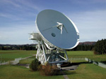
The 30-meter antenna, as shown in the opening graphic, is the main core of this verification facility. This antenna is based on a shaped Cassegrain system with elevation over azimuth mount, with higher than 50-dB gain and a beam width around 0.5° at L-band. The absolute position accuracy of this antenna is 0.001° in each direction. The signals are directed from the parabolic main reflector to the measurement cabin via a hyperbolic sub-reflector, a waveguide, and a second flat sub-reflector. One big benefit of this construction is the direct access to the installed feed in the cabin and the possibility to place the complete measurement equipment next to the feed, avoiding long connection cables.

The signals are recorded with BaySEF and for individual frequency bands (selected by switchable band pass filters) and also with a vector signal analyzer (VSA) of at least 80 MHz bandwidth. Moreover, a signal with up to 300 MHz bandwidth can be recorded with a digital oscilloscope, if the VSA is used for down conversion. Interfaces to other measurement equipment, such as navigation receivers, have already been prepared for future extension. The whole setup is referenced to a highly stable cesium frequency standard. We essentially use the BaySEF equipment as a high-capacity multiband bit grabber in this setup.

Figure 4: GIOVE-B E1 CBOC received power frequency asymmetry on May 11, 2008

The main BaySEF applications are the verification and monitoring of GNSS SIS and support for the design of applications based on parametric software-receiver evaluations. The key features most relevant for the signal-quality assessment discussion of this article are:
- Simultaneous processing (down conversion, etc.) and synchronized recording of up to four frequency bands;
- 3-dB RF bandwidth of more than 100 MHz at E5 and more than 50 MHz in other bands (E5a, E5b, L2, E6, E1);
- Maximum recording capacity of 120 megabytes per second per frequency band;
- Flexible decimation and quantization;
- Recording capacity of 0.6 terabytes per frequency band, corresponding to more than 80 minutes at the maximum recording rate;
- Remote control of data acquisition from, for example, the EADS Astrium premises in Ottobrunn.
Figure 5: GIOVE-B E1 CBOC received power flux on July 3, 2009

Figure 6: GIOVE-B E1 CBOC received power frequency asymmetry on July 3, 2009.

Figure 7: Scatter plot of GIOVE-B L1-CBOC (black crosses indicate ideal constellation).

Measurement Calibration

Accurate system calibration is the key to reliable signal quality measurements. To achieve a combined absolute measurement uncertainty significantly less than 1.0 dB (required for EIRP assessments), it is essential to calibrate precisely every used part of the system. In addition to all RF components of the receiving system, this also includes the high-gain antenna itself.

For the characterization of the high-gain antenna, two values are assessed: antenna pointing accuracy and gain. A pointing offset of about 0.04° was measured exactly with a known L-band pilot signal from the Artemis satellite and corrected in the antenna control. For gain characterization over the complete L-band frequency range of interest, the radio “star” Cassiopeia A is used. Cas A (actually a supernova remnant) is one of the strongest wide-band radio emitters in the northern hemisphere. With the help of the well-known flux density of Cas A, the gain-to-noise-temperature ratio (G/T) can be measured. After precise determination of the system noise temperature, T, the antenna gain, G, itself can be found.

For online calibration of absolute gain drifts in the measurement system, a frequency-and-power-stabilized signal generator is used in combination with two power meters.

The relative frequency transfer distortions of the receiving system are calibrated with two techniques. A network analyzer periodically provides precise measurements of gain and phase of the RF path from the antenna feed to the measurement devices.

To include also down-converting measurement devices such as the BaySEF, the injection of wide-band calibration signals is used, and simultaneously measured with a commercial digitizer (VSA).

The desired in-band measurement system transfer characteristic (relative to the VSA-characteristic, which is assumed to be ideal) is then extracted by means of de-convolving the calibration signal sampled by the device to be calibrated with the VSA-sampled reference signal.

Corresponding transfer characteristics obtained for the RF path (from network analysis) and for the BaySEF (from wide-band calibration signals) were combined to derive the equalization filter applied in post-processing the recorded samples.

Power Measurement Results

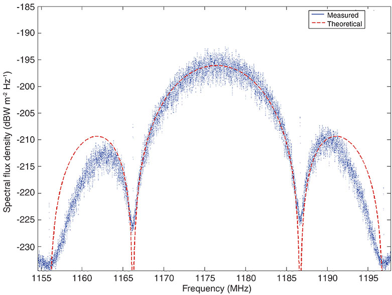
For analysis of the transmitted signal power of the GIOVE-B E1 CBOC and its variation, we have recorded a large number of spectral measurements over single satellite passes. A typical example of a single power spectral density measurement — here normalized to unit power — is shown in FIGURE 2, overlaid on the ideal spectral envelope. After absolute power calibration, we integrate the spectral power flux density over a reference bandwidth of 40.92 MHz and over the individual main lobes of the BOC(1,1) and BOCc(15,2.5) components, as illustrated in Figure 2. This procedure is used to detect the variation of transmitted signal power and possible signal asymmetries over time.

Parameter results are shown first for an early satellite pass during the IOT campaign on May 11, 2008 in FIGURE 3. Main variations in this figure are as typically expected from the cut of the measurement pass through the satellite antenna pattern. Also, the overall main-lobe power of the BOC(1,1) and the BOCc(15,2.5) components are similar, but with a strong asymmetry between upper and lower main-lobe power of the BOCc(15,2.5) component.

A closer look at the time-dependency of this asymmetry is given in FIGURE 4, showing a stable low power difference of about 0.2 dB between the BOC(1,1) main lobes and a mean power difference of 0.8 dB between the BOCc(15,2.5) main lobe with ±0.2 dB variations over time.

The second record was captured more than a year later, with similar results as shown in FIGURE 5, which indicate a stable transmission power. Only the mean main-lobe asymmetry of the BOCc(15,2.5) signal, as shown in FIGURE 6, is slightly smaller and with a different shape in its time-dependency. The measurement passes surely provided different cuts through the satellite antenna pattern. Therefore, we assume that these variations mainly indicate some antenna-pattern frequency dependency, as will be emphasized also in the following signal quality measurement results. For precise characterization, measurements and evaluations for many more satellite passes would be required.

Figure 8: GIOVE-B E1 correlation function shape of CBOC components

Figure 9: GIOVE-B E1 correlation function shape of BOCc(15,2.5) component

Figure 10: GIOVE-B E1 example of correlation-loss results for COBC-B

Signal Quality Results

In this section, we will show some GIOVE-B E1 signal quality results as obtained from BaySEF measurement data collected at Weilheim. The results presented are from two passes with the satellite in E1 CBOC-transmission mode:
- May 9, 2008, a few days after the signals were switched on
- September 29, 2008, a pass when the satellite was in eclipse for one hour.
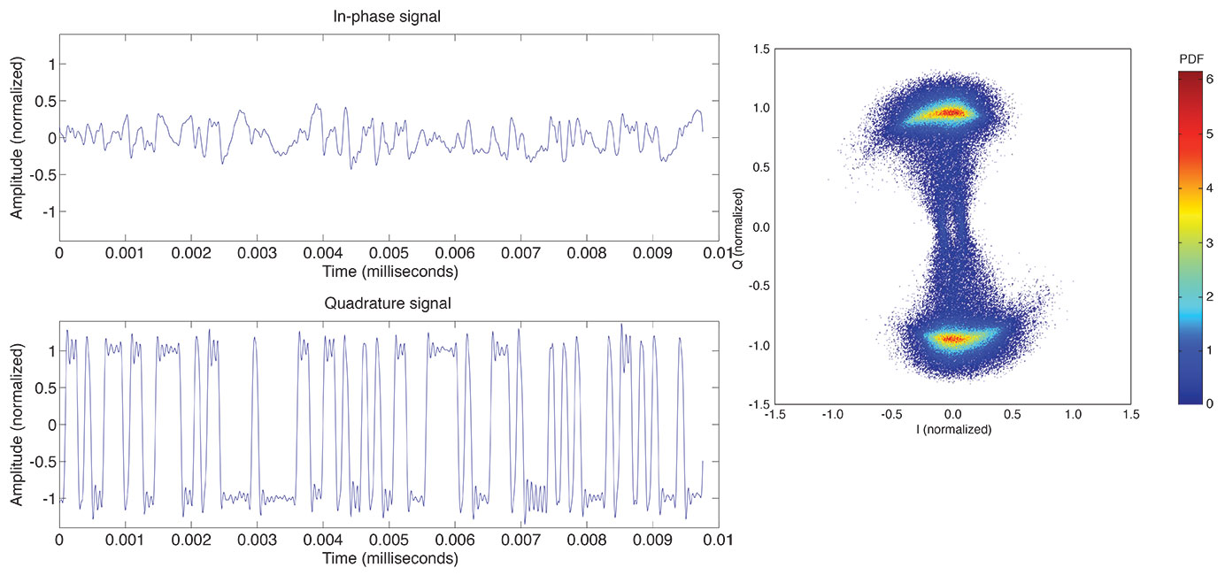
The modulation type of the E1 signal can be seen from the scatter plot, shown in Figure 7, which is derived from about 50 millisecond-signal-samples after Doppler removal. The overlay, with the eight phase points of the ideal constant envelope signal, allows clear identification of the interplexed CBOC signal. Due to bandwidth limitation, distortions, and noise jitter, the individual phase states have been enlarged, and transition traces become visible. Also, the symmetry of phase states becomes slightly deformed. How much this affects measurable navigation performance is not directly obvious from such a plot.

A better indicator of navigation performance is the E1 interplex CBOC correlation function shapes as shown in FIGURE 8 (CBOC-B and -C) and FIGURE  9 (BOCc(15,2.5)), respectively. As for all the following evaluations, the E1 signals were brick-wall band-limited to 40.92 MHz (40 × 1.023 MHz), which was the performance bandwidth of interest, and up-sampled to a rate of 575 MHz. The differences in shapes are not due to distortions but due to different signs of the BOC(6,1) subcarrier in the B and C channels. Note the imaginary part due to signal distortions has been amplified 10 times to stress its presence.

For the shape of the BOCc(15,2.5) correlation function, a small asymmetry in the real part is visible when compared to the ideal band-limited autocorrelation function. This signal distortion effect might be relevant, leading to a higher chance for false lock in acquisition and tracking. However, current receivers have no problems in tracking these signals.

A direct visual assessment of these shapes does not allow us to draw many conclusions. More quantitative evaluations provide the performance parameters of correlation-loss and lock-point-bias behavior.

Example results of the correlation-power evaluation for the GIOVE-B CBOC-B signal component are shown in FIGURE 10, with the red curve showing the correlation power of succeeding code periods relative to the total signal (which also includes the CBOC-C and BOCc(15,2.5) signal components). A curve of similar shape, shown in blue, is obtained for the ideal reconstructed signal using the specified codes and actual data bits of all components synchronized to the input signal. Obviously, the strong jitter of more than 0.1 dB is due to code cross-correlations. The correlation loss is obtained by taking the difference (see Figure 10b), which has a much lower variation with a maximum value of about 0.02 dB. This variation is still dominated by residual distortion differences of the code-cross-correlation values of the GIOVE-B codes as can be seen when accounting for the fact that equally colored dots in the figure correspond to equal code cross-correlations. Despite the variation, the negative loss is remarkable. This corresponds to a gain in usable signal power relative to the ideal case and is due to a stronger bandwidth limitation. This analysis indicates that the signal power of the wide-band signal component, BOCc(15,2.5), is more strongly reduced than for the narrow-band CBOC component, providing effectively a gain in relative correlation power for CBOC.

Next, we consider the lock-point bias of a noncoherent power discriminator as a function of early-late spacing (over the relevant range) for the CBOC-C signal component in FIGURE 11, evaluated for about 60 succeeding code periods. Again, different colors indicate different code-cross-correlation values. The corresponding S-curve bias is obtained by evaluating the peak-to-peak variation of this lock-point bias and is shown in FIGURE 12. Over this short period of 0.5 seconds, a quite stable value of about 1325 picoseconds is obtained with only 25 picosecond standard deviation mainly due to residual code-cross-correlation effects and residual noise.

Figure 11: GIOVE-B E1 example of lock-point bias dependency on early-late spacing for CBOC-C

It should be noted that all evaluation results include not only the satellite distortions but, in general, measurement distortion contributions. In fact, accurate measurement system calibration is one of the most critical issues for exact signal quality assessment of satellite transfer characteristics.

Mutual evidence of successful calibration is gained from the fact that similar results for correlation loss and S-curve bias of the CBOC-signal components have been obtained from measurements carried out by ESA together with Surrey Satellite Technology and the Science and Technology Facilities Council at the Chilbolton Observatory near Andover, England. However, even for the same measurement periods and perfect calibration, identical results may not be expected, as will be discussed here.

Figure 12: GIOVE-B E1 example of S-curve-bias evaluation result for CBOC-C

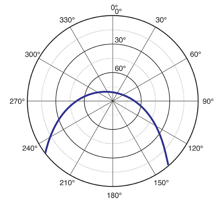
In addition to the signal-quality assessment of individual snapshot measurements, variation over observation direction and over time is of major relevance. Therefore, these evaluations have been performed for many snapshots of two single passes almost five months apart. The passes and measurement points mapped to the directions as seen from a satellite-antenna-fixed coordinate system are shown in Figure 13.

In FIGURE 14, the results of correlation loss and S-curve bias are shown for both passes mapped to the satellite antenna off-axis angle. For a monotonic x-axis, a sign was added to this angle here, with negative values for the ascending part of the pass and positive values for the descending part as seen from Weilheim.

Figure 13: GIOVE-B measurement points of BaySEF transformed into satellite antenna coordinates (off-axis angle, antenna-azimuth angle)

Figure 14: GIOVE-B E1 correlation-loss variation results over satellite passes.

The correlation-loss results for both passes vary about ±0.1 dB around 0.7 dB for BOCc(15,2.5), around -0.5 dB for CBOC-C and around -0.55 dB for CBOC-B. Also, the measured S-curve-bias results are in the same range for both passes, which is about ±100-200 picoseconds around 1200 picoseconds for CBOC-B and CBOC-C and ±2 picoseconds around 23 picoseconds for BOCc(15,2.5). Furthermore, these plots show smooth variations over the antenna off-axis angle, obviously also with some azimuth dependency due to the different shapes for each pass. It is remarkable that the relative shapes of the correlation-loss and S-curve-bias plots are so similar.

Even if measurement system instability may be a contributing factor, most of the variations are thought to be due to the directional dependency of the satellite antenna pattern. See also the similarity of results from both passes at the one end of the high off-axis angles, corresponding to similar azimuth angles. These results indicate that for full characterization of signal quality over the satellite antenna pattern, further well-calibrated measurements over several passes would be required.

During the measurement pass of September 29, 2008, a few measurement points were taken when the satellite was in eclipse. Corresponding results marked by black points in the figures show almost no impact of the eclipse on correlation loss and S-curve bias. Further measurements and evaluations would be required to confirm finally that the larger changes afterwards are not due to the eclipse.

Conclusions
This article described some of the GIOVE-B navigation SIS performance characterizations carried out by DLR and EADS Astrium in collaboration with ESA during the past year. These characterizations were achieved using a very accurate measurement system, calibrated in absolute power, relative amplitude, and phase over several frequency bands. For this purpose, several calibration approaches have been adopted and are still being optimized.

The similarity of results from measurements spaced several months apart indicates excellent long-term stability of the considered characteristics. Also, it has been demonstrated that a satellite-eclipse period seems not to affect modulation and correlation quality in a relevant manner.

As expected and already known from previous work, the satellite provides some frequency-dependent directional variations in its transmitted signal power characteristics, which also affects signal quality.

During the described campaign, the observed variations can be considered as moderate. A continuation of the monitoring activity is under consideration, to further improve the coverage of the characterizations.

During these GIOVE-B measurements and evaluations, all involved teams gained considerable experience in accurate characterization of the navigation signals transmitted from the satellite, and the operation of instruments and signal evaluation was thoroughly verified and cross-validated. The knowledge and experience gained will be very useful for future navigation satellite validation campaigns.

Acknowledgments
We would like to thank DLR’s German Space Operations Center for use of the Weilheim antenna and the colleagues who operate and maintain it. BaySEF is part of the BayNavTech program, which is supported by the Bavarian Government (Ministry for Economic Affairs, Infrastructure, Transport and Technology). The activity reported in this article was performed under a bilateral agreement between ESA and DLR’s Institute of Communication and Navigation on the exploitation of GIOVE satellites and the GIOVE signal-quality-characterization effort has been supported by ESA. This article is based on the paper “One Year in Orbit – GIOVE-B Signal Quality Assessment from Launch to Now” presented at the European Navigation Conference GNSS 2009, held in Naples, Italy, May 3–6, 2009.

Manufacturers
Measurement equipment included a Rohde & Schwarz GmbH & Co. KG (www.rohde-schwarz.com) FSQ26 vector signal analyzer. The EADS Astrium facility did not use commercial receivers to capture the GIOVE-B signals discussed in this article.

MATTHIAS SÖLLNER is senior expert on navigation signal engineering. CHRISTIAN KURZHALS and WOLFGANG KOGLER are navigation signal engineers focusing on payload aspects and performance verification, respectively. All are working at the Astrium GmbH subsidiary of the European Aeronautic Defence and Space Company N.V. (EADS).

STEFAN ERKER and STEFFEN THÖLERT work on GNSS validation and signal analysis at the German Aerospace Centre in Oberpfaffenhof-en with MICHAEL MEURER, who is responsible for performance issues concerning the Galileo system.

MAKTAR MALIK is the payload system manager for GIOVE-B at the European Space Research and Technology Centre in Noordwijk, The Netherlands, where he works with MANUELA RAPISARDA, who is a radio navigation engineer providing system support to the Galileo Project Office.

Further Reading: Click here for references related to this article.
September 1, 2009
Innovation: Where Is GIOVE-A Exactly?

Using Microwaves and Laser Ranging for Precise Orbit Determination

By Erik Schönemann, Tim A. Springer, Michiel Otten, and Matthias Becker

Though Galileo’s GIOVE-A is a test satellite not necessarily ready for scientific use, orbit analyses with a reduced accuracy can help to identify weaknesses and suggest improvements. This month, the authors share work being carried out to precisely determine the orbit of GIOVE-A using SLR and microwave observations. This preliminary investigation will benefit the procedures to be implemented for the future Galileo constellation.

INNOVATION INSIGHTS by Richard Langley

WE USE THEM FOR LISTENING TO MUSIC, for routine surgeries, for making a point in a presentation, and even for hanging pictures straight. Of course, I’m talking about lasers. Invented in 1960, the laser (an acronym for light amplification by the stimulated emission of radiation) has become ubiquitous in modern society. Every CD and DVD player has one. Many printers use them. But lasers are also used in a wide range of industrial and scientific applications including determining the orbits of satellites through satellite laser ranging (SLR).

In the SLR technique, pulses of laser light from a ground reference station are directed at satellites equipped with an array of corner-cube retroreflectors, which direct the pulses back towards a collocated receiving telescope. By accurately measuring the two-way travel times of the pulses and knowing the location of the station and other operating parameters, the positions of the satellites can be determined. A network of SLR reference stations around the globe is used to monitor the orbits of satellites over time and their variations have been used by scientists to improve our knowledge of the Earth’s gravity field; to study the long term dynamics of the solid Earth, oceans, and atmosphere; and even to verify predictions of the General Theory of Relativity.

The first SLR measurements were obtained from the Beacon Explorer-B satellite, which was launched in October 1964. Since then, dozens of satellites equipped with corner-cube retroreflectors have been launched including a number of radio-navigation satellites. Every GLONASS satellite is equipped with retroreflectors and two GPS satellites have been equipped—SVN35/PRN05 and SVN36/PRN06. The COMPASS-M1 satellite in medium Earth orbit carries retroreflectors, as do both GIOVE-A and –B, the Galileo test satellites.

Precise orbit determination of radio-navigation satellites using SLR has the advantage of being unaffected by any onboard satellite electronics and associated signal biases. Radiometric observations of a satellite’s microwave signals, on the other hand, are influenced by the satellite’s clock, for example, and its effect must be estimated to obtain precise (and accurate) satellite orbits for navigation and positioning. Therefore, a comparison of SLR- and microwave-derived orbits can be very useful for studying the performance of the data measurement and orbit-determination processes of both techniques.

In this month’s column, we take a look at some work being carried out to precisely determine the orbit of the GIOVE-A test satellite using SLR and microwave observations. This preliminary investigation will benefit the procedures to be implemented for the future Galileo constellation.

“Innovation” is a regular column that features discussions about recent advances in GPS technology and its applications as well as the fundamentals of GPS positioning. The column is coordinated by Richard Langley of the Department of Geodesy and Geomatics Engineering at the University of New Brunswick, who welcomes your comments and topic i deas. To contact him, see the “Contributing Editors” section on page 6.

The navigation office of the European Space Operations Centre (ESOC) is engaged in various activities using observations of the Galileo test satellite, GIOVE-A (Galileo In-Orbit Validation Element-A), recorded at the Galileo Experimental Sensor Stations (GESS). The work includes the assessment of the quality and performance of GIOVE satellite observables and the testing and improvement of orbit-determination software. These activities support the long-term goal of advancing the scientific applications of the future Galileo constellation.

Since the launch of GIOVE-A on December 28, 2005, various tests have been carried out to analyze the quality of the new code (pseudorange) and carrier-phase observables derived from tracking the satellite’s microwave signals. All of these tests demonstrate the advantages of the new signal structure compared to that of legacy GPS signals. In general, the reduction of the noise by factor of 4-5 as well as a reduction of the code multipath by approximately a factor of 1.2 (GPS C1C versus GIOVE-A C1B/C1C) could be seen.

As the comparison of observations is done indirectly (GPS and GIOVE-A have different orbits) and the databases used for most analyses published up to now is sparse, a deeper analysis of the signal quality parameters seems appropriate, especially as data quality has a direct impact on the precision of orbit determination. Our analyses, presented in the first half of this article, are based on a broad base of data from most of the stations in the GESS network. Because of the difficulty in accessing the phase multipath directly, we first evaluated the signal strength and the code multipath, which gave the first hint of the multipath behavior. In order to compare GPS and GIOVE-A data directly, only data received from the same elevation angles and azimuths were used. Subsequently, we present an analysis of the phase residuals derived by precise point positioning.

The second part of this article focuses on the precise orbit determination or POD of the GIOVE-A spacecraft. The Navigation Package for Earth Observation Satellites (NAPEOS) software used at the ESOC Navigation Support Office allows microwave (radiometric) and satellite laser ranging (SLR) observations to be used either separately or together. The two methods are different due to different tracking networks and the different sensitivity of the observables to atmospheric effects and in their noise levels. We will present the orbit results focusing on internal orbit consistency checks and SLR validation of the microwave-based orbits.

Data Analysis

We first describe the procedures used for analyzing the microwave data followed by those used for the SLR data.

Microwave Analysis. For the GIOVE-A signal analysis and precise orbit determination we used the RINEX data from all of the GESS stations available from the GIOVE archiving facility (see TABLE 1). All stations are equipped with GPS/Galileo antennas, built by Space Engineering S.p.A. and Galileo Experimental Test Receivers (GETRs), built by Septentrio. The data, containing tracking data of all GPS satellites and the GIOVE-A satellite, is given in the RINEX 3.00 data format with a sampling interval of 1 second. To save on storage space for the long-term analyses, such as orbit determination, the RINEX data is decimated to 30-second samples and Hatanaka-compressed, using a test version of the Hatanaka software for the RINEX 3.00 format.

The signal analyses shown here were carried out using GNU Octave, an open-source program for performing numerical computations similar to Matlab, and different scripts developed by the Institut für Physikalische Geodäsie at the Technische Universität Darmstadt. These analyses cover a selection of the designated Galileo signals recorded by the GESS within the time span from December 16 to 27, 2006. Within this time period, the current GPS signals, as well as the GIOVE-A signals E1 and E5, shown in TABLE 2, were recorded. The table also shows the signal components as well as the RINEX observation-type identifiers, which we use in this article.

The stations used for the analyses show a quite similar level of performance in general. There are stations with different behaviors for single signals, as for example GIEN with a stronger code multipath behavior on C1B and C1A, but no station with a considerably different performance level could be identified. The averaging over the data from all sites reduces the station-dependent effects such as multipath and the atmosphere to a large extent, and gives a good indication of the mean signal performance.

The analyzed phase residuals were taken from the processing carried out for the second part of this article. Hence, they include observation data over an extended period of 149 days and were limited to the GIOVE-A C1C/L1C and C7Q/L7Q signals.

This extended data period is from December 12, 2006 (day of year 346), until May 26, 2007 (day of year 146). During this interval, there is a period where no GIOVE-A data was available due to maintenance of the spacecraft. This gap occurred from February 12 to 28, 2007. So in total we have analyzed 149 days of microwave data. Because there are some differences between the results before and after this gap in February, many of the statistics are given for the first and second part separately. The first part covers December 12, 2006, until February 11, 2007; the second part covers March 1, 2007, until May 26, 2007.

We performed the precise orbit determination using the NAPEOS software, a general-purpose software package for orbit determination, prediction, and control, supporting all phases of an Earth-observation mission in terms of mission preparation and operations.

For the GIOVE-A analysis, the three main NAPEOS programs we used are GnssObs, Bahn, and Multiarc. GnssObs reads, cleans, and decimates the RINEX data and converts the data into the NAPEOS internal tracking-data format. The NAPEOS tracking-data format contains the ionosphere-free linear combination, for both code and phase, of the RINEX observations. For GPS, the ionosphere-free linear combination is based on the combination of C1P and C2P code and L1P and L2P phase measurements. GIOVE-A offers several different observables allowing for many different ionosphere-free observations. For most of the work presented in this article, we have used the ionosphere-free linear combination of the C1C and C7Q and L1C and L7Q observations for code and phase respectively.

The next module, Bahn, performs the parameter estimation. In this step, we use the ionosphere-free code and phase observations at a sampling interval of 5 minutes, and we have applied an elevation angle cut-off of 5 degrees. The data is processed in batches of 24 hours, thus resulting in 1-day-arc solutions. The estimated parameters in these daily solutions are the GIOVE-A state vector (position and velocity), five dynamical orbit parameters from the extended Center for Orbit Determination in Europe (CODE) orbit model, a GIOVE-A clock offset for each epoch, all receiver clock offsets for each epoch, one GPS-GIOVE-A “intersystem bias” parameter per day for each station except for a selected reference station, and the carrier-phase ambiguities (integers not resolved). The station coordinates are estimated but tightly constrained (1 millimeter) to their a priori value. We obtained the a priori station coordinates by combining the full set of daily solutions.

Despite the fact that the 13 GESS stations provide very good global coverage, it is expected that 24-hour solutions will not give the most precise GIOVE-A orbit estimates. To generate longer arc solutions, we have used the Multiarc program. This is a tool that has recently been added to the NAPEOS software package. It allows for a rigorous combination of normal equations, also referred to as normal equation stacking, which are generated by Bahn. During the normal equation combination, the satellite orbit parameters may also be rigorously combined, thus effectively leading to multi-day orbital arcs. For the work presented in this article, we have used Multiarc to generate solutions with arc lengths of 1, 2, 3, 4, and 5 days. We also used Multiarc to compute accurate a priori station coordinates by stacking all available 1-day normal equations.

Satellite Laser Ranging

Besides the 13 GESS stations, GIOVE-A is also tracked by more than 17 different SLR stations around the world. For most periods of the mission, the tracking has been consistent enough to allow for GIOVE-A POD using only the SLR data. As the SLR data is completely independent of the microwave data, the resulting orbit solutions will be to a large extent independent as well and thus can be used to give an indication of the achieved precision of the different microwave solutions.

The orbit determination strategy used for the SLR solutions is very similar to the one used for the microwave orbits with the main difference being the increased arc-length of 7 days. The same satellite parameters are estimated as with the microwave solutions: the GIOVE-A state vector and five dynamical orbit parameters from the extended CODE orbit model. No further parameters need to be estimated and all corrections applied to the SLR data are according to the International Earth Rotation and Reference Systems Service 2003 standards and, for station coordinates, we used those from the rescaled International Terrestrial Reference Frame 2005 solution. As the noise level of the SLR data is very low, the measurements can also be directly used to give an indication of the precision of the radial position components of the different microwave solutions by computing the SLR residuals without using them in the estimation process itself.

Combined Microwave and SLR Analysis. In this step, the SLR data was added to the microwave data in the 24-hour solutions. For the data weighting, we used 100 millimeters for SLR and 1000 millimeters and 10 millimeters for GIOVE-A and GPS code and phase observables respectively. The only change in the analysis strategy in this case was that we now processed the SLR data in 24-hour solutions and not in 7-day batches. All the processing options remained as described in the two previous sections. The resulting 1-day solutions, or rather the associated normal equations, were used in Multiarc to generate combined solutions of different arc lengths.

Microwave Data Quality

We now take a detailed look at the quality of the microwave data in terms of signal-to-noise ratio (SNR), code-tracking noise and multipath, carrier-phase-tracking noise, and carrier-phase residuals.

Signal-to-Noise Ratio. The SNR (or equivalently carrier-to-noise-density ratio, C/N₀) is strongly dependent on the satellite transmitter, the signal path through the atmosphere, and the receiver configuration (ground station, antenna, receiver, cable, etc.). Hence the SNR cannot be seen as an absolute value. The SNR is specific to the position, the equipment, and the time. Furthermore, the determination of the SNR values depends on the receiver and the firmware used. As a result, SNR values from different receivers cannot be readily compared. Nevertheless, using only one type of receiver, assuming similar effects on all the different signals at the same epoch, and taking averages over a long time span, we expect the relationships among the signals to be constant. Based on this assumption, we can use the SNR values given in the GESS RINEX files without adjustment.

To compare the GPS with the GIOVE-A SNR values, we ordered the corresponding SNR values of all stations on all days by satellite position into a grid with widths of 5 degrees in azimuth and 5 degrees in elevation angle. For the evaluation, we took the grid cells occupied by both GPS and GIOVE-A values and computed the median over all the cells of equal elevation angle. The median per elevation-angle bin for each signal is shown in FIGURE 1.

FIGURE 1. Signal-to-noise ratio, GPS versus GIOVE-A

As can be seen from the figure, the signal strength of the GIOVE-A C8Q observable ranks best, followed by the GPS C1C, GIOVE-A C7Q, C5I/C5Q, C1A, and C1B/C1C. The weakest signal is found for the GPS C1P/C2P observable, with a maximum signal strength of 40 (receiver-dependent unit, approximately dB-Hz) at the zenith. Comparing the GPS open signals versus GIOVE-A, GPS C1C is considerably stronger than the GIOVE C1B/C1C. According to the GPS and Galileo interface control documents, GIOVE-A C1B/C1A should show up with a stronger signal strength than GPS C1C. The power levels guaranteed on the Earth’s surface are -160 dBW for GPS and -158 dBW for the future Galileo satellite signals except for the BOC(10,5) and BOC(n,m) modeled signals, for which a power level of even -155dBW is guaranteed. But looking at the SNR values shown in Figure 1, we see that the GIOVE-A C1B/C1C is worse by approximately 4 dB than the GPS C1C. But keeping in mind that GIOVE-A is an experimental satellite, an increase of the signal power for the future operational Galileo satellites should improve the signal performance above that shown in this article.

Code-Tracking Noise. For signals containing data and pilot components, as in the case of those from GIOVE-A, the code-tracking noise can easily be computed as the difference between the data and the pilot signal. The advantage of this computation scheme is that both signals are influenced by identical error sources (atmospheric errors, multipath errors, receiver errors, etc.). Based on the assumption of equal uncertainties in the two components, we divided the resulting noise values by the square root of two to specify the noise level of each part according to the laws of error propagation. TABLE 3 shows the code-tracking noise for the two analyzed GIOVE-A codes sorted by elevation angle. The median code-tracking noise is 0.62 meters for C1B/C1C and 0.35 meters for C5I/C5Q, for observations below an elevation angle of 5 degrees. For the C1B and C1C code measurements, the noise median stays below 0.2 meters for an elevation angle above 25 degrees, whereas the median for the C5I and C5Q code measurements for elevation angles above 35 degrees even comes down below 0.1 meters. The results discussed above are consistent with the code-tracking noise values published previously.

Code Multipath. We computed the relative code multipath effects as code minus phase differences assuming the amplitude of phase multipath to be insignificant compared to the amplitude of the code multipath. Ionospheric effects were taken into account by using the phase measurements on two frequencies in the usual way:

In this equation, CMP_x is the estimate of the multipath error on the code, P_x and L_x are the code and phase measurements of the same frequency, while L_y is the phase measurement used to correct the frequency-dependent ionospheric effect. The constant, , describes the relationship of the ionospheric behavior for the two frequencies.

In order to compare the code multipath level of GPS versus GIOVE-A, we sorted the multipath values using a grid covering the sky with widths of 5 degrees for both elevation angle and azimuth as before. FIGURE 2 shows the median standard deviation of the code multipath values, derived in each grid cell per day and station, versus the elevation angle. No significant difference between GPS C1C and GIOVE-A C1B and C1C, the open code signals on G1/E1, could be found. The code multipath behavior of the GPS precise codes are comparable with the GIOVE-A C5I, C5Q, and C7Q, whereas the C8Q shows the least code multipath effects closely followed by the GIOVE-A C1A, the public regulated service signal.

FIGURE 2. Code multipath, GPS versus GIOVE-A

Carrier-Phase-Tracking Noise Analyses. In the same manner as that carried out with the code, we computed the GIOVE-A carrier-phase-tracking noise as the difference of the two components (pilot minus data). To accommodate the effect of error propagation, the resulting errors were divided by the square root of two. The resulting phase-tracking noise values were sorted by elevation angle and can be found in TABLE 4.

In conformity with the theory that the phase-tracking noise is independent of the modulation scheme, both signals (L1B/L1C and L5I/L5Q) show the same results in units of cycles. Looking at the results in units of distance, GIOVE-A L1B/L1C shows up with a mean phase noise of 0.7 millimeters and L5I/L5Q with 0.9 millimeters. These values confirm those of previous studies.

Carrier-Phase Residuals. Phase residuals contain the phase tracking noise, multipath, as well as all unmodeled remaining errors such as antenna calibration inaccuracy and tropospheric effects. The magnitude of the residuals can be seen as an indicator for the observation and model accuracy as well as for measurement quality.

The following analyses are based on the ionosphere-free linear combination (GPS L1C/L2P, GIOVE-A L1C/L7Q), computed with NAPEOS. The analyses include data of the 13 GESS over a period of 149 days.

To compare the GPS and GIOVE-A residuals, we sorted them into a grid with a width of one degree in both satellite azimuth and elevation angle. Only data in overlapping grid locations were compared to make sure the data was affected in a similar way by multipath or other disturbances.

To properly interpret the results, we should mention that for GIOVE-A, 0.06 percent of the ambiguities (2501) were not fixed correctly whereas for GPS all ambiguities were fixed correctly. Looking at the GIOVE-A observations that were correctly fixed, we find a significantly larger number of rejected observations. The number of rejected observations is less by one third for GPS (6 percent) as for the GIOVE-A (9 percent) data.

Due to the small number of GIOVE-A observations for elevation angles above 86 degrees, the outlier-cleaned mean as well as the standard deviation at this elevation-angle range are not meaningful. For all elevation angles, GIOVE-A residuals show a lower standard deviation than GPS, indicating a superior performance of GIOVE-A signals.

Phase and Code Validation in Processing. Looking at the quality of the code and phase measurements on the different signals, it is conspicuous that GIOVE-A C1A/L1A and C8Q/L8Q rank best, whereas for the current processing of GIOVE-A data, usually the C1C and C7Q signals are used. This leads to the question of which is the best signal combination for GIOVE-A. Hence, we processed 10 days of GIOVE-A data, using different signal combinations. Presently the processing of the C8Q/L8Q signals is not yet implemented in NAPEOS. However, we were able to process the GIOVE-A C1A/L1A – C7Q/L7Q combination. The root-mean-square (RMS) of the code results were reduced by a factor of approximately 1.4 using L1A/C1A compared to L1C/C1C, whereas the RMS of the phase observations showed only a minor improvement. Furthermore, there is a higher number of rejected observations with L1A/C1A. Further analyses have to be carried out to evaluate the potential benefits of the different signal combinations.

Orbit Quality

In this section, we assess the quality of our precise orbit determination solutions. We have three sets of different orbit solutions. Set 1 is made up of the 7-day solutions based solely on SLR observations. Set 2 consists of the solutions based on the microwave observations using 1- to 5-day arcs. Set 3 consists of the solutions based on a joint analysis of the microwave and SLR observations also using 1- to 5-day arcs.

First, we assess the orbit quality by looking at the internal consistency of the solutions. For the two sets using microwave observations, the internal orbit consistency is done using an orbit fit. This will not tell us much about the absolute quality of the solutions but it will indicate the optimal arc length and whether adding the SLR observations to the microwave data improves the orbit estimates.

Secondly, we validate the orbits by determining the SLR residuals. Of course, the solutions that used SLR observations should perform better than the microwave-only solutions. However, the validation of the microwave orbits against the SLR observations will give us a good impression of the absolute accuracy of our orbits.

As a third test, we compare the best orbit (best arc length) of each of the three sets (set 1 only has one arc length) against each other. This should give us another indication of the quality of the orbits.

Internal Orbit Consistency. To determine the internal orbit consistency of the different solutions we make an orbit fit. For this orbit fit test, we used the middle 24 hours of two consecutive solutions and fit one 48-hour arc through these two parts. The satellite orbit was modeled by estimating the satellite state vector and all nine parameters of the extended CODE orbit model. The RMS of this fit gives us an indication of the internal consistency of the orbit estimates. For longer arcs, the RMS of fit should go down because the solutions are not fully independent of each other. So a lower RMS for the longer arc solutions is expected. On the other hand, this means that if the RMS does not go down with increasing arc length that we have reached the limit of our modeling capabilities. Furthermore, comparing the internal orbit consistencies of equal length solutions will tell us which solution has a better internal consistency. The results of this internal orbit consistency check are given in TABLE 5. The table gives the mean of the 2-day RMS over all processed days. The mean is given separately for the first and second part of the observation interval (see above) and also for the total observation interval.

Table 5 shows several interesting results. First of all, it shows that the results of part 2 of the observation interval are significantly better than the results from part 1. The reason for this is unclear since the statistics from the 1-day solutions, such as the residual RMS and number of observations, did not change significantly after the observation gap. The improvement, however, is very significant. The second observation is that the results including the SLR data are significantly better compared to those using only the microwave data. This is true for all arc lengths! As expected, we see a significant improvement of the internal consistency when going from 1-day arcs to 3-day arcs. The 4-day arcs show only a slight improvement compared to the 3-day arcs. The 5-day arcs do not show a significant improvement. This indicates that with the current observations and modeling techniques, the optimal arc length for precise orbit determination seems to be around 3 to 4 days.

SLR Validation. In this section, we look at the SLR residuals obtained from the different orbit solutions. We generated a clean SLR dataset by using the SLR-only orbit to remove any outliers in the SLR observations. The total number of valid SLR normal points for the entire period is 3520 observations from 17 different SLR stations. (A normal point is an average of a number of individual laser returns.) The number of observations for the first part of the observation period is 796 points from 12 stations and for the second part, there were 2724 normal points from 17 stations. For two of the three solutions, the SLR data has been used in the orbit determination process so the residuals will give a too-optimistic indication of the orbit quality.

As can be seen from TABLE 6, the 3-day solution based on the microwave-only data has the lowest SLR residuals and indicates a radial precision of around 100 millimeters. A similar behavior can be seen in the microwave plus SLR solution with the exception of the 1-day solution (and to a smaller extent also the 2-day solution) where the orbit solution is mainly driven by the SLR data, but the quality as can be seen from the internal consistency of the orbit is poor. Interestingly, there is a large improvement in SLR residuals for the microwave plus SLR solution, although the number of SLR data points is only 2 percent of the total tracking data in the combined solution. The values for the SLR-only solution are included in the table to give an indication of the lowest possible SLR residuals one could expect by combining the microwave and SLR data.

Orbit Comparison. To get an indication of the overall orbit quality, the best solutions were compared against each other for the second period of observation. TABLE 7 gives the RMS differences between the SLR only (SLR), 3-day microwave only (micro), and the 3-day microwave and SLR solution (micro+SLR) for the radial, along-track, and cross-track position components as well as the norm (3D).

As expected, the largest difference is between the SLR-only and microwave-only solutions giving a total (norm) orbit difference of 652 millimeters. As a major part of the SLR tracking from GIOVE-A comes from European stations, the quality of the SLR solutions is directly correlated with the ability of the European stations to track GIOVE-A. Bad weather over Europe can lead to data gaps for more than 24 hours, affecting the orbit quality. It is interesting to see the large impact the SLR data has on the combined solution. As mentioned before, the SLR data is only around 2 percent of the total tracking data but has a significant impact on the orbit solution as can be seen from the difference between the microwave-only and microwave-plus-SLR solution.

Based on the analysis presented above, we conclude that the 3-day solution using both microwave and SLR observations has provided the best orbit estimates.

Conclusion

The analyses of the observation data quality (signal quality) confirmed the good results from prior analyses for code multipath behavior and code noise. GPS C1C and the GIOVE-A C1B/C1C show a comparable multipath behavior, whereas the GPS precise codes C1P/C2P are comparable to the GIOVE-A C5I, C5Q, and C7Q. The least code multipath behavior could be found for GIOVE-A C8Q observable, closely followed by the GIOVE-A C1A. Based on this, the combination C1A/L1A – C8Q/L8Q should show the best noise behavior within the data processing scheme.

The results given in this article demonstrate that the 13-station GESS network allows us to determine the orbit of the GIOVE-A satellite quite accurately (~200 millimeters) using only microwave observations. The SLR validation of the microwave orbits gives an RMS of 100 millimeters (one-way range RMS). This result gives an absolute value for the orbital error. Of course, the SLR observations mainly tell us something about the radial orbit errors; the along- and cross-track errors could be much higher. To obtain accurate GIOVE-A orbit estimates, we need to keep the orbits and clocks of the GPS satellites, tracked simultaneously with the GIOVE-A satellite, fixed using the International GNSS Service (IGS) final orbit and clock products. Furthermore, an arc length of 3 days should be used. The microwave-based orbit estimates may be improved by adding the available SLR observations into the orbit-estimation process. Although there are relatively few SLR observations, they do have a significant positive effect on the orbit estimates, improving the internal consistency from 52 to 41 millimeters. Also, the validation of the orbits using the SLR observations shows a significant improvement. However, this is not an independent validation because the same SLR observations were used in the orbit determination.

The results presented in this article, even though based on observations from the GIOVE-A test satellite, can be considered as a first attempt towards establishing an optimal data processing approach for the future Galileo satellite constellation.

Acknowledgments

This article is based on the paper “GIOVE-A Precise Orbit Determination from Microwave and Satellite Laser Ranging Data – First Perspectives for the Galileo Constellation and Its Scientific Use” presented at the 1st Colloquium on the Scientific and Fundamental Aspects of the Galileo Program, held in Toulouse, France, October 1-7, 2007.

ERIK SCHÖNEMANN studied geodesy at the Technische Universität Darmstadt (TUD), Germany, writing his diploma thesis at the University of New South Wales, Sydney, Australia. Since receiving his diploma from TUD in April 2005, he has been working for the Institute of Physical Geodesy at TUD on GNSS station calibration and validation and analyses of GIOVE-A and GIOVE-B data.

TIM SPRINGER received his Ph.D. in physics from the Astronomical Institute of the University of Berne (AIUB) in 1999. He has been a key person in the development of the Center for Orbit Determination in Europe, one of the IGS analysis centers, located at AIUB. Since 2004, he has been working for the Navigation Support Office (NSO) at the European Space Operations Centre (ESOC) of the European Space Agency (ESA) in Darmstadt. In this group, he has led the development of the new ESOC GNSS software, which is used for most GNSS activities at NSO including GIOVE-A and -B analyses.

MICHIEL OTTEN obtained a degree in aerospace engineering from Delft University of Technology in 2001. He has been working for ESOC’s NSO since 2002. His main role within NSO is the precise orbit determination of low Earth-orbiting satellites equipped for SLR, DORIS, and GPS tracking. He is also responsible for ESA’s International DORIS Service Analysis Centre activities.

MATTHIAS BECKER is a full professor of geodesy and director of the Institute of Physical Geodesy, TUD. He received his diploma and Ph.D. in geodesy from TUD in 1979 and 1984, respectively. He is responsible for research and teaching in the fields of physical geodesy and satellite geodesy.

FURTHER READING

• GIOVE-A
“Meet GIOVE-A: Galileo’s First Test Satellite” by E. Rooney, M. Unwin, A. Bradford, P. Davies, G. Gatti, V. Alpe, G. Mandorlo, and M. Malik in GPS World, Vol. 18, No. 5, May 2007, pp. 36–42.

“Galileo Signal Experimentation” by M. Hollreiser, M. Crisci, J.-M. Sleewaegen, J. Giraud, A. Simsky, D. Mertens, T. Burger, and M. Falcone in GPS World, Vol. 18, No. 5, May 2007, pp. 44-50.

• GIOVE Tracking Network
“GIOVE Mission Sensor Station Receiver Performance Characterization: Preliminary Results” by M. Crisci, M. Hollreiser, M. Falcone, M. Spelat, J. Giraud, and S. La Barbera in Proceedings of Navitec 2006, the 3rd ESA Workshop on Satellite Navigation User Equipment Technologies, Noordwijk, The Netherlands, December 11-13, 2006.

• GIOVE Tracking Performance
“Performance Assessment of Galileo Ranging Signals Transmitted by GSTB-V2 Satellites” by A. Simsky, J.-M. Sleewaegen, M. Hollreiser, and M. Crisci in Proceedings of ION GNSS 2006, the 19th International Technical Meeting of the Satellite Division of The Institute of Navigation, Fort Worth, Texas, September 26-29, 2006, pp. 1547–1559.

“Code and Carrier Phase Tracking Performance of a Future Galileo RTK Receiver” by T. Pany, M. Irsigler, B. Eissfeller, and J. Winkel in Proceedings of ENC-GNSS 2002, the European Navigation Conference, Copenhagen, Denmark, May 27-30, 2002.

• Multipath Mitigation in Modernized GNSS
“Comparison of Multipath Mitigation Techniques with Consideration of Future Signal Structures” by M. Irsigler and B. Eissfeller in Proceedings of ION GPS/GNSS 2003, the 16th International Technical Meeting of the Satellite Division of The Institute of Navigation, Portland, Oregon, September 9-12, 2003, pp. 2584–2592.

• GIOVE Orbit Determination
“Estimation and Prediction of the GIOVE Clocks” by I. Hidalgo, R. Píriz, A. Mozo, G. Tobias, P. Tavella, I. Sesia, G. Cerretto, P. Waller, F. González, and J. Hahn in Proceedings of the 40th Annual Precise Time and Time Interval (PTTI) Meeting, Reston, Virginia, December 1-4, 2008.

• Satellite Laser Ranging
“GIOVE’s Track: Satellite Laser-Ranging Campaigns” by M. Falcone, D. Navarro-Reyes, J. Hahn, M. Otten, R. Piriz, and M. Pearlman in GPS World, Vol. 17, No. 11, November 2006, pp. 34–37.

“The International Laser Ranging Service: Current Status and Future Developments” by W. Gurtner, R. Noomen, and M.R. Pearlman in Advances in Space Research, Vol. 36, No. 3, 2005, pp. 327–332 (doi:10.1016/j.asr.2004.12.012).

“Laser Ranging to GPS Satellites with Centimeter Accuracy” by J.J. Degnan and E.C. Pavlis in GPS World, Vol. 5, No. 9, September 1994, pp. 62–7.

July 1, 2009
Innovation: GPS L5 First Light

A Preliminary Analysis of SVN49’s Demonstration Signal

By Michael Meurer, Stefan Erker, Steffen Thölert, Oliver Montenbruck, André Hauschild, and Richard B. Langley

Great excitement surrounds the activation of a new transmitter from a satellite — an occasion dubbed first light. Research groups around the globe joined the GPS Wing in monitoring and analyzing the first L5 signals from space. We describe the equipment and procedures used to capture and analyze SVN49’s signals and give an assessment of their characteristics.

INNOVATION INSIGHTS by Richard Langley

ON APRIL 10, a new type of radio signal was transmitted from space. I am referring, of course, to the L5 demonstration signal from the Block IIR-M satellite SVN49, launched on March 24. The L5 signal, the second of two new civil GPS signals, will be standard on the next generation of GPS satellites — the Block IIFs — and its frequency band was duly registered with the International Telecommunication Union (ITU) back in 2002. But satellite operators only have seven years after filing a frequency application to start transmitting signals from the designated orbit, and delays in launching the first Block IIF satellite meant that GPS could lose the allocation. The GPS Wing and its contractors determined that the best way to secure the L5 frequency was to add an L5 demonstration payload to one of the remaining modernized Block IIR satellites. And so SVN49 made history with the inaugural broadcast of L5 with just a few months to spare before the clock ran out on the ITU filing.

Great excitement always surrounds the first photons captured by a new telescope or other detectors of electromagnetic signals. Or when a transmitter is activated for the first time. Just as we do for the dawning of a new day, we call this occasion first light. Research groups around the globe joined the GPS Wing in monitoring and analyzing the first L5 signals from space, including a group of scientists and engineers from Germany and Canada. This month the group describes the equipment and procedures used to capture and analyze SVN49’s signals and gives an assessment of their characteristics.

“Innovation” features discussions about advances in GPS technology and applications as well as fundamentals of GPS positioning. The column is coordinated by Richard Langley of the Department of Geodesy and Geomatics Engineering, University of New Brunswick. To contact him, see “Contributing Editors.”

A key feature of GPS modernization is the addition of the L5 civil signal to the suite of signals transmitted by the satellites. The introduction of such a signal on a different carrier frequency than that used by the legacy L1 GPS signal was proposed in the 1995 reports by the U.S. National Research Council and the National Academy of Public Administration on the future of GPS. The reports argued that an unencrypted signal on a second frequency would offer civil users the benefit of ionospheric delay correction, wide-lane carrier-phase ambiguity resolution, improved interference rejection, and faster accuracy recovery in multipath environments.

Studies showed that it would be possible to add a civil signal on the L2 frequency without compromising the military signal. High-precision (and accuracy) civil users had been using the L2 frequency — initially designated for military use only — ever since the first GPS satellites were launched, and through clever (though suboptimum) tracking techniques even after the L2 signals were encrypted. An unencrypted signal on L2 would bring these users a more robust signal as well as affording all civil users the benefits of a second frequency. But unlike the L1 signal, the L2 signal is situated in a part of the radio spectrum not officially protected from interference by other users of the spectrum. So such a second civil signal could not be used for safety-of-life applications such as navigating aircraft.

So, in Vice President Al Gore’s statement of March 30, 1998, on the enhancement of GPS for civil users, the decision to deploy two new civil signals was announced: the civil signal on L2, now known as L2C, and a signal on a new frequency, which became known as L5. Some readers might wonder why this new signal was not designated L3 or L4. Those designations had already been assigned to signals associated with other payloads on the GPS satellites.

Although the Gore announcement proposed to introduce both of the new civil signals with the launch of the Block IIF satellites, the addition of the L2C signal to the legacy signals was deemed a relatively straightforward task and the decision was made to modify the last eight Block IIR satellites for the provision of L2C. The first modernized Block IIR satellite was launched on September 26, 2005, and seven of these satellites are now in orbit.

The frequency selected for the L5 signal, 1176.45 MHz, is in a protected aeronautical radionavigation services (ARNS) band. This frequency, as with frequencies used by all satellite operators, had to be coordinated with the International Telecommunication Union-Radiocommunication Sector (ITU-R). The ITU-R registers frequencies essentially on a first-come, first-served basis, but a user must actually transmit signals on the assigned frequency from the designated satellite orbit type within seven years from the date of filing with ITU-R. This meant that L5 signals had to be transmitted before August 26, 2009, to avoid the potential claim of the frequency by a different country. A decision was made to modify an existing Block IIR-M satellite to carry an L5 demonstration payload. The L5 demo payload, which was developed by Lockheed Martin and its subcontractors, was added to space vehicle number (SVN) 49. SVN49 was launched on March 24, 2009, the seventh modernized Block IIR satellite to be placed in orbit. Also known as PRN1, from the primary pseudorandom noise (PRN) codes assigned to the satellite, the satellite began L5 transmissions on April 10, at 11:58 UTC, and so satisfied the ITU-R filing requirement with a few months to spare.

The L5 Signal Structure

The structure of the future full L5 signal will differ significantly from the legacy L1 signal or even the modernized L2C signal. It is fully described in the Navstar GPS L5 interface document, IS-GPS-705. We present just a brief overview of the signal here.

Two-Component Signal. The full L5 signal will offer two signal components: one with and one without a superimposed navigation data message. The two signal components — in-phase (I) and quadrature (Q) — have equal power. Both will have a minimum received power of –157 dBW. Each component is modulated with a different, but synchronized, L5 PRN code. The in-phase component (the I- or data channel) is further modulated with a 100-symbol per second (sps) symbol stream carrying the navigation message data, and the quadrature component (the Q- or data-free channel, also called the pilot channel) is modulated only with a PRN code. Different, nearly orthogonal PRN codes (referred to as I5 and Q5) are used in the two components to prevent tracking biases by making each component completely independent of the other, except for the underlying carrier phase.

Another novel aspect of the L5 signal design is the use of Neuman-Hoffman (NH) synchronization codes.

Code Structure. As previously mentioned, the I5 and Q5 channels are modulated with different PRN codes. These codes differ significantly from the C/A-, P-, and L2C-codes used on L1 and L2 both in length and chipping rate.

The natural code chipping-rate frequency of 10.23 MHz as provided by the SV atomic frequency standards satisfies a number of requirements for a modernized signal within the bandwidth constraints — increased bandwidth efficiency, improved signal accuracy, immunity to waveform distortion, and improved rejection of narrowband interference. The bandwidth constraints include rejection of out-of-band interference. Accordingly, a 10.23 megachip per second (Mcps) chipping rate, 10 times that of the C/A- and L2C-codes, was adopted for the L5 PRN codes.

Improved Cross-Correlation. There is a trade off between code period and the capability to do direct acquisition. A longer code period provides better cross-correlation properties, but takes longer to search. However, one can speed up an acquisition to some extent with lower code cross-correlation levels.

The L1 C/A-code period is 1023 chips, or 1 millisecond. The desire to maintain that epoch rate of 1 kHz with the 10.23 Mcps chipping rate results in a code period of 10,230 chips. For both the I5 and Q5 ranging codes, the 1-millisecond sequences are the modulo-2 sum of two sub-sequences referred to as XA and XB with lengths of 8,190 and 8,191 chips, respectively. The same XA sequence is used for both I5 and IQ, whereas the XB sequence for I5 is different from that for Q5. The XB sequences are selectively advanced to produce different 1-millisecond-long code sequences. In this way, a large number of unique codes can be generated. Thirty-seven primary code pairs have been designated, of which 32 are reserved for use by GPS satellites (PRNs 1–32). An additional 173 pairs have been defined (PRNs 38–210). PRN sequences 38 through 63 are reserved for satellites.

Demo Signal Verification

The L5 signal transmitted by SVN49 contains only the dataless quadrature component modulated with the PRN63 Q5 sequence. Furthermore, the transmitted L5 signal power and the satellite antenna radiation pattern are different from those expected for the L5 signals to be transmitted by the Block IIF satellites as described in the L5 interface specification.

Over the past few weeks, the German Aerospace Center (Deutsches Zentrum für Luft- und Raumfahrt or DLR) has monitored SVN49 using its GNSS verification and analysis facility. The core element of the facility is a 30-meter dish antenna at Weilheim, near Munich, Germany, and is shown in FIGURE 1. The antenna, which is based on a shaped Cassegrain system, has a 30-meter-diameter parabolic reflector and a hyperbolic sub-reflector with a diameter of 4 meters. The L-Band gain of this high-gain antenna is around 50 dB, with a beam width of less than 0.5°. The position accuracy in both azimuth and elevation directions is 0.001°. The antenna’s maximum slewing speeds are 1.5° per second in azimuth and 1.0° per second in elevation angle, allowing it to easily track MEO satellites.

FIGURE 1. GNSS verification and analysis facility with 30-meter high-gain antenna at Weilheim, Germany.

In September 2005, DLR’s Institute of Communications and Navigation established an independent monitoring station for the analysis of GNSS signals using this powerful instrument. For the new challenge, the antenna was adapted to the requirements in the navigation field. A newly developed broadband circularly polarized feed and a new receiving chain including an online calibration system were installed at the antenna during preparations for the GIOVE-B in-orbit test campaign in the spring of 2008.

During this time, intensive work on the system calibration was performed using well-known signals from radio “stars” and EGNOS satellites for the antenna gain determination, and sophisticated calibration methods for the receiving system. The calibration provides an absolute measurement uncertainty significantly less than 1 dB.

Due to the distance of the antenna location from the institute at Oberpfaffenhofen (around 40 kilometers), it was necessary to perform all measurement and calibration procedures during the measurement campaigns under remote control. A software tool was developed that can control any component of the setup remotely. In addition, this tool is able to perform a completely autonomous operation of the whole system by a pre-definable sequence over any period of time. Additional details about the GNSS verification and analysis facility and the calibration techniques used can be found in the literature cited in Further Reading.

A detailed signal-in-space (SIS) analysis of the new L5 signal transmitted by SVN49 was conducted by recording several passes with the GNSS verification and analysis facility. A high elevation-angle transit of SVN49 every night allows a long observation time for each satellite pass. To ensure precise tracking of the satellite with the high-gain antenna, we used the latest two-line element sets from the U.S. Air Force Space Command.

The first signals transmitted by the satellite on the L5 frequency were captured during the pass on April 10. Compared to later measurements, the power of the L5 payload signal was measured with a lower output level on this first pass. This points to a power “fade in,” which is a common procedure in commissioning a new satellite payload. A controlled and slow heating of the payload elements avoids possible damage caused by the out-gassing of the power amplifiers, for example.

The SIS analyses that we performed using the high-gain antenna will be described for one example satellite pass recorded on April 29. During this pass, the satellite reached an elevation angle of around 80° and was visible for about seven hours (see FIGURE 2). A set of spectral snapshots as well as time sample records for the L1, L2, and L5 signals were processed and adjusted with the corresponding calibration values during a post-processing stage.

FIGURE 2. Skyplot of SVN49 pass at Weilheim, Germany, on April 29, 2009.

Time and Frequency. A first view of the captured spectrum snapshot in FIGURE 3 shows the L5 signal and its typical binary phase-shift-keyed (BPSK) spectral shape. The signal is significantly band limited by the used front-end filters of the satellite’s L5 payload. This ensures the required spectral separation from the adjacent L2 signal of the satellite, as the L5 signal must not interfere with the operational L2 frequency. Overlaying the theoretical spectral mask of the L5 BPSK signal, we note a slight asymmetry of the spectral shape. The two side lobes differ around 2.5 dB in their peak power level (see Figure 3). Spectral asymmetries of that kind typically result from frequency selectivity in the RF transmitter chains in satellite payloads, including the amplifiers and antennas.

FIGURE  3. L5 spectrum plot from data recorded on April 29.

FIGURE 4 shows a temporal snapshot of the L5 signal after wiping off the Doppler frequency shift due to satellite orbital motion. Figure 4 (left) depicts a snapshot of 10 microseconds for the I and Q channels. It can be seen, that in compliance with the requirements of the L5 signal explained in the introduction of this article, the signal is a bi-level signal with a chipping rate of 10.23 Mcps. Plotting the normalized histogram of the L5 signal, one obtains the normalized I/Q probability density function (PDF) diagram of the L5 signal shown in Figure 4 (right). The constellation diagram shows a remaining deformation of the Q component after Doppler removal. Although the L5 signal transmitted by the test payload only contains the dataless Q5 component, a non-negligible contribution can be seen in the I channel. This slight distortion may stem from a nonlinear and frequency-dependent amplification of the Q baseband signal leading to crosstalk between the Q and I channels.

FIGURE  4. (left) L5 I and Q time samples; (right) L5 I/Q probability density function (PDF).

Signal Code Sequence. With the use of the high-gain antenna, it is possible to look in detail at the transmitted L5 code chips. The signal is raised high above the noise floor and, after Doppler wipe off, allows us to compare the received code sequence with the theoretical code sequence for the PRN63 Q channel. FIGURE 5 shows an example for the first 10 microseconds of the code — both for the measured L5 signal and the expected theoretical code. The analysis performed also for several full code periods shows that the demo payload’s Q5 code structure is in full compliance with the “theoretical” code described in the official signal interface document.

FIGURE  5. Comparison of measured and theoretical code sequences.

Power of Received Signals. The GNSS verification and analysis facility is fully calibrated, allowing highly accurate absolute measurements of GNSS signal power levels. We have used the system to evaluate the SVN49 signal power levels as received on the ground. FIGURE 6 shows the different signals transmitted in the L1, L2, and L5 frequency bands in terms of the received power per square meter versus elevation angle of the SV during its pass. It can be seen that there is a significant elevation-angle dependency of the L5 received power (about 18 dB between low and high elevation angles) compared to L1 and L2 (with a variation of about 3 dB). In this measurement, the combined power of the I and Q channels is plotted for the signals. So this means that the L1 and L2 signal measurements include the power of the C/A-, P(Y)-, and M-codes. Such a strong elevation-angle dependency is not typical of signals radiated by GPS satellites. However, the L5 signal is radiated using the legacy L1/L2 Block IIR-M satellite antenna, which is to the authors’ knowledge not optimized for the L5 frequency.

FIGURE  6. Absolute received power for SVN49 L1, L2, and L5 signals on April 29, 2009.

In the spectrogram plot of FIGURE 7, which was generated by plotting all recorded L5 spectra versus elevation angle, the impact of this elevation-angle dependency of the received power can be detailed for the complete frequency range. The side lobes of the BPSK signal are only clearly visible in the spectrogram at higher elevation angles.

FIGURE  7. Spectrogram for L5 signal received on April 29, 2009.

Signal Tracking

In parallel with the detailed signal validation using the high-gain antenna and vector signal analyzer, an effort has also been made to track the new GPS L5 signal using conventional correlating GNSS receivers. Given the relevance of L5/E5 signals for future aeronautical applications and the ongoing transmission of such signals from the GIOVE satellites, a growing number of commercial receiver manufacturers have announced receivers supporting this frequency band. However, due to the special nature of the SVN49 test signal (pilot only, with different PRN code designations on L1 and L5) some modifications to receiver software are required to properly track the first GPS L5 signal. In particular, the use of different PRN code designations employed for L1/L2 (PRN1) and L5 (PRN63) is clearly non-standard and requires suitably adapted receiver software, which was provided by the makers of the two receiver types we selected for our test campaign.

Receiver type N is a highly configurable test receiver for L1 and L5/E5a signals developed as part of the Galileo program. It offers a total of 16 tracking channels, which are implemented in a field-programmable gate array and can thus be flexibly adapted for tracking of civil GPS, satellite-based augmentation systems, and the GIOVE-A and -B signals in their respective frequency bands. Receiver type J, in contrast, represents the latest generation of geodetic grade multi-constellation receivers. It uses an advanced application-specific integrated circuit with 216 tracking channels supporting all types of non-military navigation signals in the L1/E1, L2, and L5/E5a bands. Both receivers have been used for some time prior to the launch of SVN49 to track GPS and GIOVE satellites from stations at the University of New Brunswick (UNB) in Canada and at DLR in Germany.

The first measurements of GPS L5 were successfully collected on April 10 with a type N receiver at UNB. While these measurements confirmed the capability to properly track SVN49 in the L5 band, they already revealed a distinct aspect of the GPS L5 test signal that potential users must be aware of. The signal is much weaker at low elevation angles than the L1 signal. Normal carrier-to-noise-density ratios (C/N0) are only achieved at elevation angles of about 60° and higher. On the other hand, the measured C/N0 near zenith may even outperform that of L1 and L2 tracking with sufficient L5 antenna gain. For illustration, FIGURE 8 compares the measured C/N0 values of GPS and GIOVE-A/B signals as obtained with receiver type J and a geodetic antenna at DLR, Oberpfaffenhofen.

FIGURE  8. Comparison of the relative signals strength (expressed as carrier-to-noise-density ratio, C/N0) for GPS (left) and GIOVE-A/B signals (right). The signals are described by their respective RINEX 3.00 data format identifiers, which reflect the type of measurement (S=signal strength), the frequency band (1=L1/E1, 2=L2, 5=L5/E5a) and the signal attribute (C=C/A or L2C, W=P(Y) semicodeless, X=pilot and data).

While not officially confirmed so far, the abnormal variation of the L5 signal strength can best be attributed to a non-standard gain pattern of the satellite transmitter antenna. Apparently, the existing Block IIR-M satellite antenna “farm” has been used to transmit the L5 signal, which results in more directivity than that of the L1 and L2 signals. This results in a weaker signal for receivers further away from the antenna boresight axis, or, equivalently, stations observing the satellite at low elevation angles. Even though the achieved C/N0 of the GPS L5 test signal is lower than that of the direct L1 C/A-code and L2 L2C-code tracking for most of a tracking arc, the signal quality still exceeds that of the semicodeless P(Y)-code tracking on L1 and L2. This makes the signal a valuable basis for experimentation in aviation applications or triple-frequency processing.

To assess the quality of the raw GPS measurements, we made use of the so-called multipath combination of pseudorange and carrier-phase measurements:

The combination is essentially the difference between the pseudorange (P _C5) and carrier-phase measurement (Φ_L5) on the L5 frequency, and therefore measures the sum of the pseudorange multipath (M) and noise (ε). Due to the opposite sign of ionospheric path delays on code and phase measurements, an ionospheric correction is used in the multipath combination, which requires phase measurements on a second frequency (in this case L1). The individual carrier-phase biases are, furthermore, aggregated into a common bias (b). Other than in a traditional zero-baseline test, the multipath combination neither requires a second receiver nor a second satellite transmitting the same signal in space. It is therefore best suited for studying the tracking performance of the new GPS L5 test signal.

Results for receiver types N and J obtained at DLR, Oberpfaffenhofen, are shown in FIGURE 9 for a sample, high-elevation angle tracking pass. Despite obvious differences that can be related to the specific multipath environment and code-smoothing strategies for the two receivers, a high quality is obtained in both cases. For the central three-hour interval, during which the L5 signal was received with normal signal strength, the achieved tracking accuracy clearly outperforms that of the L1 C/A-code signal for the given receivers. For further comparison, FIGURE 10 shows sample results of GIOVE-B E5a tracking with receiver type J. Again, the GPS L5 signal at medium- to high-elevation angles is fully competitive and a notable degradation is only evident when the signal strength is well below the values to be expected in the future operational system.

FIGURE  9. Pseudorange multipath and receiver noise of SVN49 (PRN G01) L5 tracking for a selected pass over Oberpfaffenhofen, Germany, on April 29-30, 2009. Top: receiver type J with geodetic antenna. Bottom: receiver type N with a Galileo antenna. The satellite exceeded an elevation angle of 50° between 20:30 and 23:30 with a peak elevation angle of 80° near 22:00.

FIGURE 10. Pseudorange multipath and receiver noise of GIOVE-B L5 tracking for a high pass over Oberpfaffenhofen, Germany, on April 17, 2009, using receiver type J.

Legacy Signal Anomaly. While the GPS L5 signal transmission by SVN49 is clearly designated as experimental, the legacy signals (that is, the C/A- and P(Y)-code on L1 as well as L2C- and P(Y)-code on L2) were expected to achieve the same level of performance as observed on other satellites of the existing constellation. This is not the case, however, in the L1 band where both the C/A-code measurements and the semicodeless P(Y)-code pseudoranges exhibit a systematic, elevation-angle-dependent bias. This bias is not specific to any of our test receivers and can be similarly observed in heritage receivers employed at the stations of the International GNSS Service (IGS). As an example, FIGURE 11 illustrates the variation of the C/A-code error for high-elevation angle passes of SVN49 over western Canada and Germany. The bias varies between approximately -0.5 meters near the horizon and 1meter near zenith.

The cause of the bias is unclear but resides apparently in the design of the transmitter antenna or signal generation chain. It is exclusively seen on SVN49 and not on other GPS (or GIOVE) satellites, which excludes a possible problem of the receiver antenna or environment. Furthermore, data collected at UNB using the UNBJ IGS station a few days after launch clearly demonstrate that the elevation-angle-dependent L1 bias existed well before L5 signal activation and therefore might not be related to the signal generator. It is unclear to what extent the L1 signal bias can be corrected on the spacecraft and how it will affect the declaration of SVN49 as a fully healthy satellite.

FIGURE 11. Pseudorange errors of SVN49 L1 C/A code tracking for high-elevation-angle passes using a type A receiver at IGS station DRAO in Penticton, Canada (top), and a type J receiver at Oberpfaffenhofen (bottom). The satellite achieved peak elevation angles of about 70° and 80°, respectively, at the two sites.

Conclusions

Tracking and analysis of SVN49’s L5 signal using both the 30-meter dish and code-correlating receivers reveals that it possesses improved signal characteristics with respect to the legacy signals, in particular with regard to its bandwidth, and therefore will allow even more accurate and reliable positioning when the signal is deployed on the future Block IIF constellation.

Acknowledgments

We thank NovAtel and JAVAD GNSS for supplying special firmware, Sébastien Carcanague at UNB, and DLR colleagues at Weilheim for their help. The L5 signal description comes from the Innovation article by A.J. Van Dierendonck and C. Hegarty, September 2000 issue of GPS World.

Manufacturers

Receiver N is the NovAtel (www.novatel.com) EuroPak-15a. Receiver J is the JAVAD GNSS (www.javad.com) Triumph Delta-G2T. Receiver A is an Allen Osborne Associates (AOA) Benchmark ACT (www.itt.com). Space Engineering (www.space.it) Galileo Experimental Sensor Station antenna, Trimble (www.trimble.com) Zephyr Geodetic II antenna, and AOA D/MT antennas were used.

MICHAEL MEURER received a Ph.D. in electrical engineering from the University of Kaiserslautern, Germany. He is director of the Department for Navigation in the Institute for Communications and Navigation of the German Aerospace Center (DLR).

STEFAN ERKER received his diploma degree in information technology from the Technical University of Kaiserslautern and works at DLR’s Institute for Communications and Navigation.

STEFFEN THÖLERT received his diploma degree in electrical engineering from the University of Magdeburg and works at DLR.

OLIVER MONTENBRUCK works at DLR’s German Space Operations Center, Oberpfaffenhofen, where he is head of the GPS Technology and Navigation Group. He holds a Dr.rer.nat degree in physics.

ANDRÉ HAUSCHILD received his diploma degree in mechanical engineering from the Technical University of Braunschweig, Germany, and is a Ph.D. candidate at DLR’s German Space Operations Center.

Further Reading

L5 Signal Details
Interface Specification, IS-GPS-705 (IRN-705-003), Navstar GPS Space Segment/User Segment L5 Interfaces, ARINC Engineering Services, LLC, El Segundo, California, September 22, 2005.
“The New L5 Civil GPS Signal” by A.J. Van Dierendonck and C. Hegarty in GPS World, Vol. 11, No.9, September 2000, pp. 64–72.

DLR’s GNSS Verification and Analysis Facility
“GNSS Signal Verification: Spectral and Temporal Analysis of GIOVE B and BEIDOU Signals” by S. Thölert, S. Erker, M. Cuntz, M. Meurer, U. Grunert, and J. Furthner, presented at Navitec 2008, the 4th ESA Workshop on Satellite Navigation User Equipment Technologies, Noordwijk, The Netherlands, December 10–12, 2008.
“GNSS Signal Verification with a High Gain Antenna – Calibration Strategies and High Quality Signal Assessment” by S. Thölert, S. Erker, and M. Meurer in Proceedings of ITM 2009, the 2009 International Technical Meeting of The Institute of Navigation, Anaheim, California, January 26–28, 2009, pp. 289-300.

Nonlinearities in Microwave Signal Components
“Frequency-independent and Frequency Dependent Nonlinear Models of TWT Amplifiers” by A. Saleh in IEEE Transactions on Communications, Vol. 29, November 1981, pp. 1715–1720.
“Analysis of GIOVE-A L1-Signals” by S. Graf and C. Günther in Proceedings of ION GNSS 2006, the 19th International Technical Meeting of the Satellite Division of The Institute of Navigation, Fort Worth, Texas, September 26-29, 2006, pp. 1560–1566.

Commercial GNSS Receivers Used for L5 Signal Acquisition
“Triumph Technology” by J. Ashjaee presented at the 5th Allsat Open Conference, Hannover, Germany, June 19, 2008.
“A Dual-frequency L1/E5a Galileo Test Receiver” by N. Gerein, M. Olynik, M. Clayton, J. Auld, and T. Murfin in Proceedings of the European Navigation Conference – GNSS 2005, Munich, Germany, July 19-22, 2005.

The Multipath Observable
“TEQC: The Multi-Purpose Toolkit for GPS/GLONASS Data” by L.H. Estey and C.M. Meertens in GPS Solutions, Vol. 3, No. 1, 1999, pp. 42–49.

1995 Reports on the Future of GPS
The Global Positioning System: Charting the Future: Charting the Future by a panel of the National Academy of Public Administration and by a committee of the National Research Council, National Academy of Public Administration, Washington, D.C., 1995, ISBN 0-9646874-1-0.
The Global Positioning System: A Shared National Asset, Recommendations for Technical Improvements and Enhancements by the National Research Council Committee on the Future of the Global Positioning System, National Academy Press, Washington, D.C., 1995, ISBN 0-309-05283-1.

The Seminal Article on the Benefits of Three GPS Signal Frequencies
“The Promise of a Third Frequency” by R.R. Hatch in GPS World, Vol. 7, No. 5, May 1996, pp. 55–58.

June 1, 2009
Solar Burst Impacts GPS

On December 6, 2006, the sun emitted a burst of radio energy that impacted the performance of GPS receivers all over the sunlit side of the Earth. That the sun produces radio emissions is not surprising. What is surprising is that on this day they were extremely powerful. The sun continuously emits energy across a broad region of the radio spectrum. The flux density of these emissions is normally fairly low and contributes imperceptibly to the background radio noise collected by GPS receiver antennas.

However, when a solar flare occurs, it is often accompanied by very powerful bursts of radio energy. Although they are more numerous near the peak of the solar sunspot cycle when the sun is more disturbed, solar flares and their associated strong radio bursts can occur at anytime – including near the current sunspot minimum. Still, the December 6 solar radio burst came as a surprise. It was one of the largest on record and had an impact on all GPS receivers on the sunlit side of the Earth, including most of North America, South America, and the Pacific Ocean. The added noise significantly reduced carrier-to-noise-densities (C/N0 – a measure of the strength of received signals) at both the L1 and L2 frequencies by as much as 15 dB-Hz. This resulted in receivers losing lock on some satellites for many minutes, particularly those at low elevation angles with low C/N0 values before the burst’s arrival. Those receivers closer to the sub-solar point were typically affected more than those further away as more or the burst energy was picked up by the receiver antennas.

Nevertheless, it appears that a lot of single-frequency receivers continued to provide navigation solutions with as few as four satellites — and even three in 2D mode — and the noise burst went unnoticed by most users of such receivers. However, many dual-frequency receivers used for high-accuracy applications including those at reference stations suffered significant signal losses, particularly at the L2 frequency. As well, military receivers in some sectors lost the ability to navigate. A “widespread loss of GPS” in the Four Corners region of New Mexico and Colorado was reported by military authorities. Several aircraft reported losing lock on GPS signals with the number of tracked satellites dropping from 7-9 to 1 or even none!

Alessandro Cerruti, a graduate student at Cornell University, is among a group of scientists and engineers studying the effects of this and other solar radio bursts on the operation of GPS receivers. He has examined the data provided by the receivers in the International GNSS Service (IGS) network on the sunlit side of the Earth. The number of stations providing data at both frequencies on at least four satellites dropped from more than 120 to below 60 during the burst. The timing of the drop-outs coincides with the power of the burst which is shown in the lower panel.

The burst power was recorded at the Owens Valley Solar Array (OVSA) in California’s high desert. Operated by the New Jersey Institute of Technology’s Center for Solar-Terrestrial Research, OVSA records solar radio emissions at over a range of frequencies and polarizations including right-hand circular polarization (RHCP) at 1.6 GHz, very near the GPS L1 frequency. As the plot shows, noise power exceed one million solar flux units at the peaks of the burst, making this burst one of the largest on record.

Alessandro Cerruti has also looked at data from the Wide Area Augmentation System (WAAS) which is very robust and although WAAS continued to operate throughout the period of the burst, signals at the WAAS reference stations suffered significant degradations as elsewhere. The C/N0 values for PRN 4 as recorded at the Houston reference station on both the L1 and L2 frequency for a quiet day and on December 6. The drop in C/N0 values during the burst is very dramatic.

Mitigation. What can be done, if anything, to mitigate the effects of solar radio bursts? As the bursts are broadband noise, it is difficult for a receiver to discriminate them from GPS signals. Some antenna designs, such as choke rings, attenuate signals arriving at low elevation angles, so if the sun is low in the sky at the time of a burst, receivers with such antennas will be less impacted than those with conventional antenna designs. And as a receiver loses track primarily on satellites at low elevation angles, having more satellites at higher elevation angles will also help. So receivers operating with a mixed constellation of GPS and GLONASS or GPS and Galileo satellites should be better able to weather a solar radio burst than those operating with GPS alone. Similarly, a larger GPS constellation by itself would help.

Modernization. Stronger transmitted signals from future GPS satellites might allow receivers to continue tracking even low-angle satellites during a large burst. Newer signal formats, which could be tracked at lower C/N0 values, would also help receivers to contend with the sun’s outbursts. Even current receiver technology developed for anti-jamming protection and for indoor GPS use would allow receivers to track to much lower C/N0 values and perhaps sail through even very strong solar radio bursts.

As we approach the peak of the next sunspot cycle in 2012, we can expect more solar radio bursts. Some forecasts peg the next peak at 30–50 percent stronger than the last one as measured by the fraction of the sun’s visible hemisphere with sunspot activity. Will future solar radio bursts have as dramatic an effect as the burst of December 6, 2006? Time will tell.

— Richard Langley

April 27, 2007
Innovation Catalog

A catalog of all Innovation columns published in GPS World from Vol. 1, No. 1 (1990) to Vol. 21, No. 12 (2010). Download the PDF.

January 1, 1990