Author: Richard B. Langley

  • Innovation: Record, Replay, Rewind

    Innovation: Record, Replay, Rewind

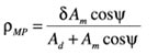
    Testing GNSS Receivers with Record and Playback Techniques

    By David A. Hall

    Is there a way to perform repeatable tests on GNSS receivers using real signals? This month’s column looks at how to use an RF vector signal analyzer to digitize and record live signals, and then play them back to a GNSS receiver with an RF vector signal generator.

    INNOVATION INSIGHTS by Richard Langley
    INNOVATION INSIGHTS by Richard Langley

    AS A PROFESSOR, I’m quite familiar with testing — of students, that is. It’s how we check their performance — how well they have mastered the course material. Outside academia, testing is also quite common. We have to pass a driving test before we can get a license. We might have to pass a physical fitness test before starting a job. And manufacturers have to test or stress their products to make sure they are fit for purpose. As David Ogilvy, the father of advertising once quipped, “Never stop testing, and your advertising will never stop improving.” But it’s not just manufacturers who should test products. Consumers, or their representatives, should test products on offer — not only to corroborate (or dispute) manufacturers’ claims but also to compare one manufacturer’s product against another. There’s a whole slew of magazines, television programs, and web resources devoted to testing and comparing everything from laundry detergent to automobiles. And GNSS receivers are no exception.

    When we conduct tests, we are usually trying to get answers to certain questions — just like those posed to students on their exams. In testing GNSS receivers, what are some appropriate questions? When a receiver is turned on, how long does it take until the position of the receiver is determined? When a weak signal area is encountered, can the receiver still determine its position? If the signal is interrupted and then restored, how long does it take for the receiver to recover and resume calculating its position? And what is the position accuracy under different situations?

    While we can certainly hook up an antenna to a receiver to get answers to these questions in a certain environment on a certain day at a certain time with certain signals, the scenario cannot be repeated — not exactly. If we tweak a receiver operating parameter, for example, we don’t know for certain whether any observed change is due to the tweaking or a change in the scenario. We could use a radio-frequency (RF) simulator — a device for mimicking the radio signals generated by the satellites. This would allow us to define scenarios, including receiver trajectories, and to replay them as many times as necessary while varying the operating parameters of the receiver. Or we could modify the scenario from run to run. Such test scenarios could include those difficult to carry out with live signals such as determining how a receiver would perform in low Earth orbit. While extremely useful, these are tests with simulated signals.

    Is there a way to perform repeatable tests on GNSS receivers using real signals? In this month’s column, we learn how to use an RF vector signal analyzer to digitize and record live signals, and then play them back to a GNSS receiver with an RF vector signal generator — a procedure we can repeat as often as we like.


    While GNSS simulators have long provided the de facto technique for testing GPS receivers, radio frequency (RF) record and playback has emerged as an innovative method to introduce real-world impairments to GNSS receivers. In this article, we will provide a hands-on tutorial on how to test a navigation device using the record and playback technique.

    The premise of RF record and playback is to capture GNSS signals off the air with a vector signal analyzer (VSA) and then replay them to a receiver with an RF vector signal generator (VSG). With recorded GNSS signals, one is able to introduce a signal that contains natural impairments — instead of an ideal signal — to the GNSS receiver. As a result, one can observe how a receiver will behave in a real-world environment where interference, multipath fading, and other impairments are present.

    A VSA combines traditional superheterodyne radio receiver technology with high-speed analog-to-digital converters and digital signal processors to perform a variety of measurements on complex modulated signals. It is widely used in the telecommunications industry as a test instrument. Digitized signals can be recorded for future analysis. A VSG reverses the process, taking a digital representation of a complex waveform and, using digital-to-analog converters, generating an appropriately modulated RF signal.

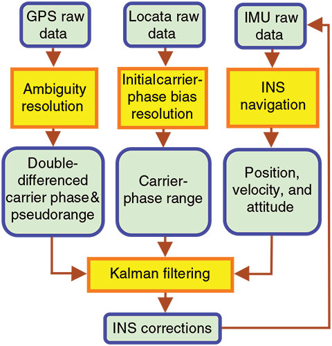
    Recording GPS or GLONASS signals off the air can be done in a fairly straightforward manner. An RF recording system combines appropriate antennas, amplifiers, and an RF signal recorder (usually a VSA) to capture many hours of continuous RF signal. In such a system, the basic components include the RF front end, the RF signal-acquisition device, and high-volume storage media. A block diagram of a typical recording system is shown in Figure 1.

    Figure 1. GPS receivers implement cascaded low-noise amplifiers. The RF signal acquisition block includes analog-to- digital conversion (ADC) and digital down conversion (DDC) to select the data of interest.
    Figure 1. GPS receivers implement cascaded low-noise amplifiers. The RF signal acquisition block includes analog-to- digital conversion (ADC) and digital down conversion (DDC) to select the data of interest.

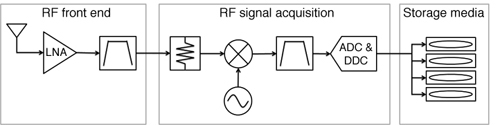
    In the figure, the RF front end is designed to condition the GNSS signal in such a way that it can be captured — with maximum dynamic range — by the recording device. The recording device digitizes a given signal bandwidth, and then stores in-phase and quadrature (IQ) waveforms to disk.

    In general, RF recording devices are designed to tune to a broad range of frequencies and can thereby record many different types of signals. Thus, selecting the signal to record is as simple as setting the center frequency and bandwidth of the recording device. For example, to record the GPS C/A-code L1 signal, the center frequency should be set to 1575.42 MHz. Because each satellite generates the same carrier frequency, one can capture C/A-code signals from all satellites simply by capturing all signals within a 2.046 MHz (twice the code chipping rate) band around the carrier frequency.

    By contrast, recording GLONASS signals requires slightly different settings. Because the GLONASS constellation uses frequency division multiplexing, every satellite generates the same code, but each pair of antipodal satellites transmits at a unique center frequency. Thus, recording L1 signal information for the entire GLONASS constellation requires a recorder to capture signals that range from 1598.0625 MHz (channel -7) to 1605.375 MHz (channel 6). In order to capture the entire bandwidth of each satellite, a recorder is actually required to capture 1.022 MHz of signal for each carrier (again, twice the code chipping rate). Therefore, the total recording bandwidth is actually 1597.5515 MHz to 1605.886 MHz, a span of 10.3345 MHz. On the RF signal analyzer, one can record GLONASS signals simply by setting the center frequency to 1601.71875 MHz, and the bandwidth to ≥ 10.3345 MHz.

    Modern RF signal recorders are capable of recording both GPS and GLONASS C/A-code signals on a single wideband recording channel. For example, one of our RF signal analyzers is capable of recording up to 50 MHz of signal bandwidth. With this instrument, one can simultaneously record both GPS and GLONASS by setting the center frequency to 1590.1415 MHz and the bandwidth to ≥ 31.489 MHz. However, while RF recording systems can be used to capture a wide range of GNSS signals including GPS L1/L2/L5, GLONASS L1/L2, Galileo, and others, this article focuses primarily on the GPS C/A-code signal.

    Setting up the RF Front End

    The trickiest aspect of recording GPS signals is the selection and configuration of the appropriate antenna and low noise amplifier (LNA). When connecting a typical off-the-shelf GPS passive patch antenna to a signal analyzer, the peak power in the GPS L1 band ranges from -120 to -110 dBm. Because the power level of GPS signals is small, significant amplification is required to ensure that the VSA can capture the full dynamic range of the signal.

    The simplest method to amplify an off-the-air GPS signal so that it can be captured by an RF signal recorder is the combination of an active GPS antenna and one or more external LNAs. Note that many professional GPS antennas offer the best performance because they combine high element gain with an LNA and even pre-selection filtering, which improves the dynamic range of the RF recorder.

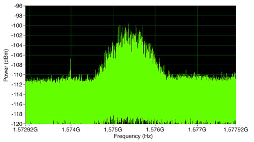
    With the RF front end appropriately configured, one can verify system performance using a simple spectrum analyzer demonstration panel. The demo panel allows one to visualize the RF spectrum in the GPS L1 band. If all is set up correctly, the C/A-code GPS signal should be visually present on the display. Figure 2 illustrates a screenshot of the spectrum on a virtual spectrum analyzer display.

    Note that visualizing the GPS signal in the frequency domain with an RF signal recorder (or spectrum analyzer) requires careful attention to settings such as resolution bandwidth and averaging. Because the signal-to-noise ratio (SNR) of the GPS signal is so small, the settings shown in Figure 2 require a narrow resolution bandwidth (10 Hz) and significant averaging (20 averages per measurement record, so a 20-second interval for 1 Hz data). With these settings applied, one can easily visualize a modulated signal above the noise floor with approximately 1 MHz of bandwidth and centered at 1575.42 MHz. This signal is the GPS C/A-code. In Figure 2, the reference level of the signal analyzer was set to -50 dBm to reduce the noise floor of the instrument to the lowest possible level. Note that setting the signal analyzer’s reference level provides a simple mechanism to adjust the front-end attenuation or amplification. In general, RF signal analyzers provide the greatest dynamic range when the reference level of the instrument matches closely with the average power of the signal connected to the front end. In this case, setting the reference level of our signal analyzer to -50 dBm removes all front-end attenuation, giving the analyzer a more optimal noise figure for signal recording.

     Figure 2. GPS is visible in the spectrum only if a narrow resolution bandwidth is used. This spectrum was obtained with a center frequency of 1575.42 MHz, a frequency span of 4 MHz, a resolution bandwidth of 10 Hz, root-mean-square averaging with 20 averages, and a reference level of 250 dBm.
    Figure 2. GPS is visible in the spectrum only if a narrow resolution bandwidth is used. This spectrum was obtained with a center frequency of 1575.42 MHz, a frequency span of 4 MHz, a resolution bandwidth of 10 Hz, root-mean-square averaging with 20 averages, and a reference level of 250 dBm.

    Hardware Connections

    With the reference level appropriately set, it is important to properly configure the RF front end of the recording device. As previously mentioned, one can achieve the best RF recording results by using an active GPS antenna. The active antenna used in our experiment utilized a built-in LNA to provide up to 30 dB of gain with a 1.5 dB noise figure. (Recall that the noise figure is the difference in dB between the noise output of a device and the noise output of an “ideal” device with the same gain and bandwidth when it is connected to sources at the standard noise temperature — usually 290 K.) However, the LNA must be powered by supplying a DC bias to the RF connection. While there are several methods to supply the DC bias, we will look at two of the easiest methods.

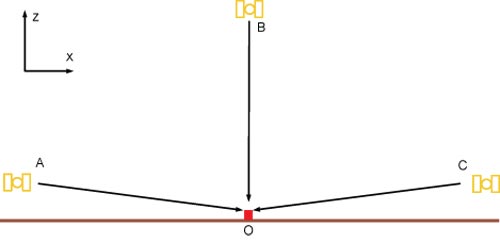
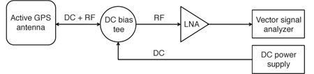
    Method 1: Active Antenna Powered by GPS Receiver. The first method to power an active antenna is with a bias tee or DC power injector. Using this three-port component, a DC voltage (3.3 V in this case) is fed to its DC port, which applies the appropriate DC offset to the active antenna connected to the RF-in port while blocking it on the RF-out port. The device gets its name from the fact that the three ports are often arranged in the shape of a “T.” Note that the precise DC voltage one should apply depends on the DC power requirements of the active antenna. A diagram illustrating the connections is shown in Figure 3.

    Observe in Figure 3 that one can use off-the-shelf hardware such as a programmable DC power supply to supply the DC bias signal. Also, one can use a generic off-the-shelf bias tee as long as it has bandwidth up to 1.58 GHz.

     Figure 3. This set-up shows the use of a DC bias tee to power an active GPS antenna.
    Figure 3. This set-up shows the use of a DC bias tee to power an active GPS antenna.

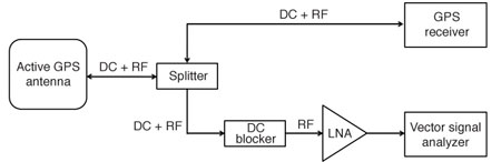
    Method 2: Active GPS Antenna Powered by Receiver. A second method of powering the active GPS antenna is with the receiver itself. Most off-the-shelf GPS receivers use a single port to power and receive signals from an active GPS antenna, and this port is already biased with an appropriate DC voltage. Combining an active GPS receiver, a power splitter, and a DC blocker, one can power an active LNA and simply record essentially the same signal as that observed by the GPS receiver. A diagram of the appropriate connections is shown in Figure 4. Some splitters incorporate a DC block on all but one of the output ports.

    As Figure 4 illustrates, the DC bias from the GPS receiver is used to power the LNA. This method is particularly useful for drive tests because one can observe the receiver’s characteristics, such as velocity and dilution of precision, while recording.

     Figure 4. With a DC blocker, one can record and analyze the same GPS signals being tracked by a GPS receiver.
    Figure 4. With a DC blocker, one can record and analyze the same GPS signals being tracked by a GPS receiver.

    Selecting the Right LNA

    Recording GPS signals with generic RF signal recorders is possible largely because external LNAs can be used to reduce the effective noise floor of the receiver. Today, one can find off-the-shelf spectrum analyzers with noise figures ranging from 15 dB to 20 dB. One of our analyzers, for example, has a 15 dB noise figure while applying up to 60 dB of gain. By applying external amplification to the front of an RF signal analyzer, however, one can substantially reduce the noise figure of the RF recording system.

    To calculate the total noise that will be added to the recorded GPS signal, one must calculate the noise figure for the entire RF front end. As a matter of principle, the noise figure of the entire system is always dominated by the first amplifier in the system. Thus, careful selection of the first and second stage LNAs is crucial for a successful signal recording.

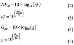
    We can calculate the noise figure of the RF recording system by using the Friis formula for noise figure, named for engineer Harald Friis, a Danish-American radio engineer who worked at Bell Telephone Laboratories. To use this formula, first convert the gain and noise figure of each component to its linear equivalent; the latter is called the “noise factor.” For cascaded systems such as our RF recording system, the Friis formula provides us with the noise factor of the entire system:
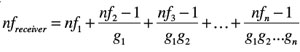
    In-E1        (1)

    Note that both noise factor (nf) and gain (g) are shown in lowercase to distinguish them as linear measures rather than logarithmic measures. The conversion from linear to logarithmic gain and noise figure (and vice v
    ersa) is shown in the following equations:

    IN-E2-5

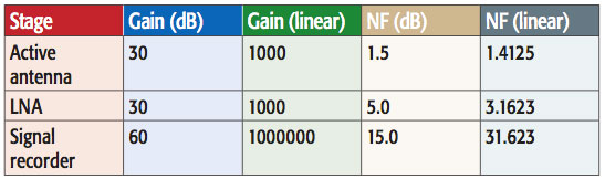
    An active GPS antenna using a built-in LNA typically provides 30 dB of gain while introducing a noise figure that is typically on the order of 1.5 dB. The second part of the recording instrumentation provides 30 dB of additional gain as well. Though its noise figure is higher (5 dB), the second amplifier actually introduces very little noise into the system. As an academic exercise, one can use the Friis formula to calculate the noise factor for the entire RF front end of the recording instrumentation. Gain and noise figure values are shown in Table 1.

    Table 1. Noise figures and factors of the first two components of the RF front end.
    Table 1. Noise figures and factors of the first two components of the RF front end.

    According to the calculations above, one can determine the overall noise factor for the receiver:

    IN-E6  (6)

    To convert noise factor into a noise figure (in dB), apply Equation 2, which yields the following results:

    IN-E7     (7)

    As Equation 7 illustrates, the noise figure of the first LNA (1.5 dB) dominates the noise figure of the entire RF recording system. Thus, with the VSA configured such that the noise floor of the instrument is less than that of the input stimulus, one’s recording introduces only 1.507 dB of noise to the off-the-air signal.

    Saving Data to Disk

    Each GNSS produces slightly varying requirements for an RF recorder’s signal bandwidth and center frequency. For the GPS C/A-codes, the essential requirement is to record 2.046 MHz of RF bandwidth at a center frequency of 1575.42 MHz.

    In the tests described here, we set the IQ sample rate of our RF recorder at 5 megasamples per second (Ms/s). Since each 16-bit I and Q sample is 32 bits (or 4 bytes each), the actual recording data rate is 20 megabytes per second (MB/s) to ensure the entire bandwidth was captured. Capturing more than 4 MHz of bandwidth is sufficient to record the 2.046 MHz C/A-code signals.

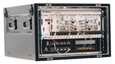
    Because one can achieve data rates of 20 MB/s or more with standard PXI controller hard drives (PXI is the open, PC-based platform for test, measurement, and control), one does not need to use an external redundant array of independent disks (RAID) volume to stream GPS signals to disk when using a PXI recording system. In general, data rates exceeding 20 MB/s require the use of an external RAID volume. External RAID systems are capable of storing more than 600 MB/s of data and can be used to support wide bandwidth channels or even multi-channel recording applications. For example, the recording system shown in Figure 5 uses an external RAID volume for high-speed signal recording. This system combines PXI RF signal generators and analyzers with external amplifiers and filter banks for a ready-to-use GNSS record and playback solution.

     Figure 5. Two-channel record and playback system from Averna.
    Figure 5. Two-channel record and playback system from Averna.

    In our tests, we decided to use a 320 GB USB drive for better portability. With a disk speed of 5400 revolutions per minute, we were able to benchmark it ahead of time and observed that we were able to achieve read and write speeds exceeding 25 MB/s. Thus, we were easily able to use this disk drive and still record IQ samples at 5 MS/s (20 MB/s) when recording off-the-air signals. With the existing hard-drive setup, we could record more than 4 hours of continuous IQ signal. Note that capturing longer recordings simply requires a larger hard disk. By using a 2 terabyte RAID volume (the largest addressable disk size in the Windows XP operating system), we can extend our recording time to 25 hours. With this setup, we could also reduce the IQ sample rate to 2.5 MS/s (still sufficient to capture the GPS C/A-code signals) and extend the recording time to 50 hours.

    Receiver Performance

    Once the off-the-air signal of a GNSS band is recorded to disk, it can be re-generated and fed to a receiver using an RF signal generator. With an RF signal generator that is able to reproduce the real-world GNSS signal, engineers are able to test a wide range of receiver characteristics. Because recorded signals contain a rich set of channel impairments such as ionosphere distortion and interference from other transmitters, design engineers often use recorded signals to prototype the baseband processing algorithms on a GNSS receiver.

    In our case, we used a VSG directly connected to a GPS evaluation board. In the experiments described below, the receiver’s latitude, longitude, and velocity were tracked over time. Data was read from the receiver using a serial port, which read NMEA 0183 sentences at a rate of one per second. NMEA 0183 is a standard protocol developed by the National Marine Electronics Association for communications between marine electronic devices. NMEA 0183 has been adopted by virtually all GPS receiver manufacturers. In our LabVIEW graphical development environment, one can parse all sentences to return satellite and position-fix information.

    For practical testing purposes, GPS dilution of precision and active satellites (GSA), GPS satellites in view (GSV), course over ground and ground speed (VTG), and GPS fix data (GGA) sentences are the most useful. More specifically, one can use information from the GSA sentence to determine whether the receiver has achieved a position fix and is used in time-to-first-fix measurements. When performing sensitivity measurements in this example, the GSV sentence was used to return carrier-to-noise-density ratios (C/N0) for each satellite being tracked. In addition, the VTG sentence allows us to observe the velocity of the receiver. Finally, the GGA sentence provides the receiver’s precise position by returning latitude and longitude information. See the references in Further Reading for in-depth information on the NMEA 0183 protocol.

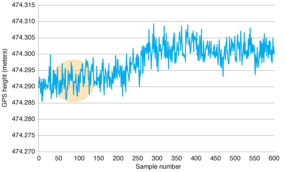
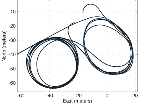
    Using the receiver’s reported latitude and longitude information, we are able to test its ability to report a repeatable position when the recorded signal is played back to the receiver. In this experiment, we tracked the receiver position over 10 minutes. For the best results, the command interface of the receiver should be tightly synchronized with the start trigger of the RF signal generator. The results in Figure 6 show that the RF vector signal generator in this experiment was synchronized with the GPS receiver by using the data line of the serial communications (COM) port (RxD, pin 2) as a start trigger. Using this synchronization method, the vector signal generator and GPS receiver were synchronized to within one clock cycle of the VSG’s arbitrary waveform generator (100 MS/s). Thus, the maximum skew should be limited to 10 microseconds. Given our receiver’s maximum velocity of 15 meters per second (our maximum speed on the drive test), we can determine that the maximum error induced by clock offset of the signal generator is 10 microseconds x 15 meters per second, or 0.15 millimeters.

    Using the configuration described above, one is able to report the receiver’s latitude and longitude over time, as shown in Figure 6.

    IN-Fig6a
    Figure 6A. Receiver latitude over a four-minute span.
    Figure 6B. Receiver longitude over a four-minute span.
    Figure 6B. Receiver longitude over a four-minute span.

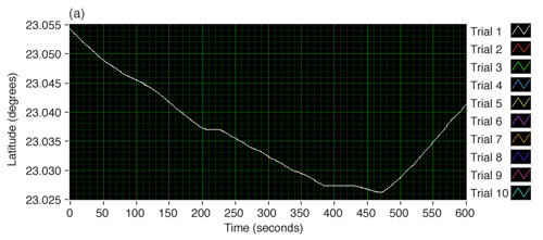
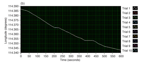
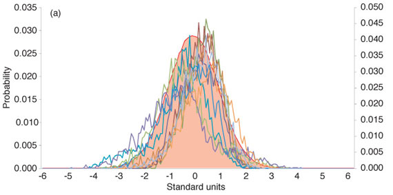
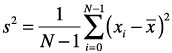
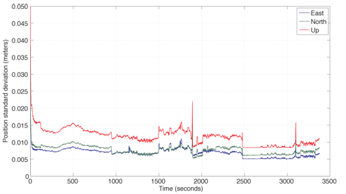
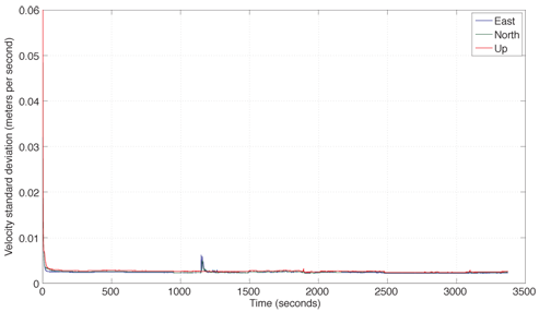
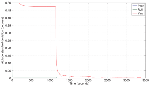
    As the data from Figure 6 illustrate, a recorded test-drive signal reports static, position, and velocity information. In addition, one can observe that this information is relatively repeatable from one trial to the next, as evidenced by the difficulty in graphically observing each individual trace. To better characterize the deviation between each trace, one can also compute the standard deviation between each sample in the waveforms. Figure 7 illustrates the standard deviation between each of the 10 trials, calculated for every one-second interval, versus time.

    FIGURE 7 Standard deviation of both latitude and longitude over time
    Figure 7. Standard deviation of both latitude and longitude over time.

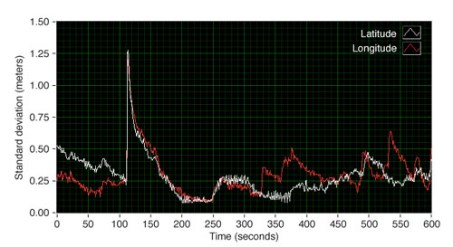
    When observing the horizontal standard deviation, it is interesting to note that the standard deviation appears to rapidly increase at time = 120 seconds. To investigate this phenomenon further, we can plot the total horizontal standard deviation against the receiver’s velocity and a proxy for C/N0. In this case, we simply averaged the C/N0 values for the four highest satellites reported by the receiver. Since four satellites are required to achieve a three-dimensional position fix, our assumption was that position accuracy would closely correlate with the signal strength of these important satellite signals.

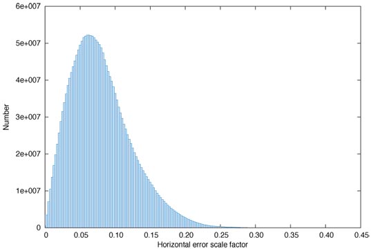
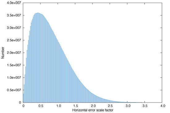
    One simple method to evaluate the horizontal repeatability of the receiver position versus time is to calculate the standard deviation on a per-sample basis of each recorded latitude and longitude (in degrees). Once the standard deviation is measured in degrees, we can roughly convert this to meters with the following equation:

    IN-E8

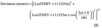
    Note that Equation 8 represents a highly simplified error calculation method, which assumes that the Earth is a perfect sphere. For a more precise calculation of repeatability, the geodesic formula (which presumes that the Earth is ellipsoidal) should be used. In our simple experiment, the goal is merely to correlate repeatability with other factors that we can measure from the receiver. Figure 8 illustrates the standard deviation of horizontal position repeatability over 10 trials and at one-second time intervals.

     Figure 8. Correlation of position accuracy and C/N0.
    Figure 8. Correlation of position accuracy and C/N0.

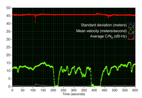
    As one can observe in Figure 8, the peak horizontal error (measured by standard deviation) occurring at time = 120 seconds is directly correlated with satellite C/N0 and not correlated with receiver velocity. At this sample, the standard deviation is nearly 2 meters while it is less than 1 meter during most other times. Concurrently, the top four C/N0 averages drop from nearly 45 dB-Hz to 41 dB-Hz.

    The exercise above illustrates not only the effect of C/N0 on position accuracy but also the types of analysis that one can conduct using recorded GPS data. For this experiment, the drive recording of the GPS signal was conducted in Huizhou, China (a city north of Shenzhen), but the actual receiver was tested at a later date in Austin, Texas.

    Conclusion

    In this article, we’ve illustrated how to use commercially available off-the-shelf products to record GPS signals with an RF recorder, and then play the signal back to a receiver. As the results illustrate, recorded GPS signals can be used to measure a wide range of receiver characteristics. Not only can receiver designers use these test techniques to better prototype a receiver baseband processor, but also to measure system-level performance such as position repeatability.

    Manufacturers

    The tests discussed in this article used a National Instruments PXIe-5663E, 6.6 GHz, RF signal analyzer; a National Instruments PXI-5690, 100 kHz to 3 GHz, two-channel programmable amplifier and attenuator; a National Instruments PXIe-5672, 2.7 GHz, RF vector signal generator with quadrature digital upconversion; a 320 GB USB Passport hard drive from Western Digital Corp.; a National Instruments PXI-4110 programmable, triple-output, precision DC power supply; and a ZX85-12G-S+ bias tee manufactured by Mini-Circuits. The article also mentioned the RP-3200 2-channel record and playback system manufactured by Averna, which incorporates National Instruments modules.


    David Hall is an RF product manager for National Instruments. He holds a bachelor’s of science with honors in computer engineering from Pennsylvania State University.


    FURTHER READING

    More on GNSS Receiver Record and Playback Testing

    GPS Receiver Testing, tutorial published by National Instruments, Austin, Texas.

    Friis Formula and Receiver Performance

    RF System Design of Transceivers for Wireless Communications by Q. Gu, published by Springer, New York, 2005.

    Global Positioning System: Signals, Measurements, and Performance, 2nd edition, by P. Misra and P. Enge, published by Ganga-Jamuna Press, Lincoln, Massachusetts, 2006.

    “Measuring GPS Receiver Performance: A New Approach” by S. Gourevitch in GPS World, Vol. 7, No. 10, October 1997, pp. 56-62.

    “GPS Receiver System Noise” by R.B. Langley in GPS World, Vol. 8, No. 6, June 1997, pp. 40–45.

    Global Positioning System: Theory and Applications, Vol. I, edited by B.W. Parkinson and J.J. Spliker Jr., published by the American Institute of Aeronautics and Astronautics, Inc., Washington, D.C., 1996.

    GNSS Receiver Testing Using Simulators

    “Testing Multi-GNSS Equipment: Systems, Simulators, and the Production Pyramid” by I. Petrovski, B. Townsend, and T. Ebinuma in Inside GNSS, Vol. 5, No. 5, July/August 2010, pp. 52–61.

    “GPS Simulation” by M.B. May in GPS World, Vol. 5, No. 10, October 1994, pp. 51–56.

    GNSS Receiver Testing Using Software

    “GPS MATLAB Toolbox Review” by A.K. Tetewsky and A. Soltz in GPS World, Vol. 9, No. 10, October 1998, pp. 50–56.

    GNSS L1 Signal Descriptions

    Navstar GPS Space Segment / Navigation User Interfaces, Interface Specification, IS-GPS-200 Revision E, prepared by Science Applications International Corporation, El Segundo, California, for Global Positioning System Wing, June 2010.

    Global Navigation Satellite System GLONASS, Interface Control Document, Navigational Radio Signal in Bands L1, L2 (Edition 5.1), prepared by Russian Institute of Space Device Engineering, Moscow, 2008.

    NMEA 0183

    NMEA 0183, The Standard for Interfacing Marine Electronic Devices, Ver. 4.00, published by the National Marine Electronics Association, Severna Park, Maryland, November 2008.

    “NMEA 0183: A GPS Receiver Interface Standard” by R.B. Langley in GPS World, Vol. 6, No. 7, July 1995, pp. 54–57.

    Unofficial online NMEA 0183 descriptions: NMEA data; NMEA Revealed by E.S. Raymond, Ver. 2.3, March 2010.

  • Innovation: Friendly Reflections

    Innovation: Friendly Reflections

    Monitoring Water Level with GNSS

    A receiver can selectively acquire scattered signals and the resulting measurements can be interpreted to reveal certain characteristics of the source of the scattering. This article discusses the design and application of a GNSS instrument that uses scattered signals for monitoring the level and roughness of inland and coastal water surfaces for the betterment of planet Earth.

    By Alejandro Egido and Marco Caparrini

    INNOVATION INSIGHTS by Richard Langley
    INNOVATION INSIGHTS by Richard Langley

    WHY IS THE SKY BLUE? This is an age-old question, interesting to anyone with a curiosity about his or her surroundings. But what has it got to do with global navigation satellite systems? Believe it or not, there is a connection.

    Some of you might remember the explanation of the sky’s color from your Physics 101 course but to bring everyone up to the same level, let’s review. Everything we see is the result of the interaction of light and matter. And by matter, we mean the atoms, molecules, and particles making up matter. Light causes matter to vibrate. And vibrating matter (due to its electrical charges) in turn emits light, which combines with the original light. But matter not only re-emits light in the forward direction, it re-emits light in all other directions. This is called scattering.

    Now, the light from the sun includes all colors and so if look directly at the sun when it is high in the sky (don’t try this at home), it looks white or slightly yellowish. We are seeing the light propagating directly toward our eyes. When we look at the sky away from the sun, we are seeing scattered light. And this scattered light is predominantly blue. Why? It turns out that scattering is proportional to the fourth power of frequency. Light that is of a higher frequency, say a factor of two, is sixteen times more intensely scattered. So, blue light, which has about twice the frequency of light from the red end of the visible spectrum, is scattered much more than red light. Violet light is scattered even more but our eyes are not as sensitive to violet light as they are to blue light. Hence the sky looks blue.

    So what has this got to do with GNSS? As we know, for the best positioning and navigation results, we need the satellite signals to travel along a direct path to the receiver’s antenna. There may be slight changes in the speed and direction of propagation of these direct-path signals caused by the interaction of the electromagnetic waves with the matter making up the ionosphere and the neutral atmosphere, but these are readily accounted for in the position fixes.

    However, once they reach the Earth’s surface, the signals can be reflected by buildings, vegetation, the ground, water surfaces, and so on. The signals are actually being scattered by the matter they encounter. A receiver can selectively acquire the scattered signals and the resulting measurements can be interpreted to reveal certain characteristics of the source of the scattering.

    In this month’s column, we learn about the design and application of a GNSS instrument that uses scattered signals for monitoring the level and roughness of inland and coastal water surfaces–yet one more use of GNSS signals for the betterment of planet Earth.


    Lakes and water reservoirs are the world’s most important sources of accessible fresh water. Despite its paramount importance — not only for a large variety of human activities, but also for the sustainability of ecosystems — fresh water is already scarce in many regions. The problem is envisaged to become worse in the coming decade. In addition, in climatological studies surface water storage is a critical element of the water cycle since the analyses integrate all hydrologic processes (precipitation, runoff, evapotranspiration, and so on) over a given basin; and for hydroelectric companies, it is the main parameter to be kept under observation for efficient energy production. All of these concerns make the monitoring of fresh water resources a prime activity for a wide variety of stakeholders including governments, climate research organizations, and hydroelectric production companies.

    Coastal management is also a wide-ranging issue with large social and economic impacts. Care of our coasts includes dealing with threats such as storm surges and flooding, coastal erosion, and conflicting land-use issues. Coastal areas support the greatest concentration of living resources and people on the planet. In the past few decades, these regions have experienced a population density increase, which is envisioned to grow steadily. Furthermore, conflicts between commercial interests, recreational activities, infrastructure development, environment conservation, and exploitation of natural resources will become increasingly important and contentious. In fact, the coastal zone is a peculiar environment in which terrestrial, oceanic, atmospheric, and human inputs of energy and matter converge. Storm surges and coastal flooding events have caused considerable damage and economic loss on European coasts in particular. Such events, possibly linked to the world climate change, are expected to get worse in the near future, due to sea level rise and storm activity.

    So, close monitoring of both inland waters and coastal regions is necessary for the well being of the planet. And since the need is so pervasive, monitoring systems should be characterized by a relatively low cost, low maintenance, and easy deployment, to serve the widest possible user community. We have developed a patent-pending solution using signals from global navigation satellite systems (GNSS).

    Called Oceanpal, our monitoring system exploits reflected GNSS signals as signals of opportunity for passive remote sensing of the Earth’s water surfaces. These multipath signals are usually considered to be nuisance signals since they reduce the accuracy of GNSS positioning applications. But for monitoring various processes affecting the Earth’s surface, they are very beneficial. The technique is known as GNSS reflectometry (GNSS-R), and during the past decade, its use as a technique for Earth observation purposes has taken root.

    GNSS-R is basically a bistatic radar technique. While most radar systems, such as those used for monitoring air space and harbor approaches and for weather forecasting, combine the radar transmitter and receiver at the same site — so-called monostatic radar — bistatic systems use transmitters and receivers separated by a considerable distance. Such systems have been used for studying certain atmospheric phenomena and for military applications where simple line-of-sight reflections from the target of interest are inadequate or insufficient.

    The concept of bistatic radar can be extended to satellite signals. Since some of the signal transmitted by a satellite gets reflected off the Earth’s surface, detecting this reflected signal by a separate passive receiver would provide some information about the reflecting surface. While any satellite signal could be used in principle, GPS (and other GNSS) turn out to be particularly useful. The concept of using GPS signal reflections was initially proposed in 1993 by Manuel Martín-Neira, working at the European Space Agency’s European Space Research and Technology Centre in Noordwijk, The Netherlands. Since then, the technique has been successfully implemented by an increasing number of researchers.

    We could list several reasons for the continuous growing interest in GNSS as a remote sensing tool, but two main ones stand out: first, the global availability and stability of GNSS signals enables their use as reliable signals of opportunity; and second, GNSS makes use of L-band radiation, which is highly interactive with the natural scattering medium but relatively impervious to atmospheric conditions. Moreover, the passive nature of this concept allows for the production of cost- and resource-effective instruments.

    Navigation signals are sensitive to a wide variety of geophysical parameters including topography, surface roughness, surface moisture, ionospheric electron content, tropospheric water vapor, water salinity, and vegetation. Research targeting related geophysical applications has been ongoing for many years, and the first pre-operational services exploiting reflected GNSS signals are now available. In fact, while the scientific community is waiting for a dedicated GNSS-R space mission to confirm the theoretical predictions about the characteristics of reflected signals observed from space, ground-based and airborne sensors have already been developed and validated for a number of applications.

    The GNSS-R research area that has been most thoroughly investigated concerns the reflection of navigation signals from water surfaces, given the highly reflective nature of water. However, from water the interest has now moved towards ice and land applications, more specifically to the detection of sea ice and the monitoring of soil moisture. Recently, GNSS-R has also been proposed as a possible tool to monitor vegetation. This article focuses on the presentation of the Oceanpal sensor, and the description of the altimetry algorithms for monitoring the levels of sea (coastal) and inland waters.

    Our Instrument

    As mentioned above, Oceanpal is a GNSS-R-based sensor designed for operational monitoring of coastal and inland waters. The instrument comprises three subsystems: a radio frequency (RF) section, an intermediate frequency (IF) section, and a data-processing section. The RF section features a pair of low gain L-band antennas. A right-hand circularly polarized (RHCP) zenith-facing antenna collects the direct GNSS signals while a left-hand circularly polarized (LHCP) nadir-facing antenna collects the sea- or lake-surface reflected GNSS signals. (On reflection, the signals become predominantly LHCP.) Data bursts of some minutes’ duration are acquired from each antenna using two GPS L1 receivers (front ends) that down-convert the signals to IF. Within the IF sections, the signals are one-bit sampled and stored on a hard disk.

    These direct and reflected raw data are then fed into the processing section of the instrument, where a pair of software GNSS receivers detects and tracks the available signals in the direct channel (which works as a master) and blindly despreads the reflected signals in the reflected (slave) channel. The result of this processing is a set of direct and reflected electromagnetic field time series for each satellite in view, plus some ancillary information, such as the satellite pseudorandom noise code (PRN) numbers and GPS time references, among others. The architecture described above is shown in FIGURE 1.

    Figure 1. Basic operation of Oceanpal and the principle of GNSS-R-based sea-surface monitoring. Right-hand and left-hand circularly polarized antennas feed signals to radio frequency (RF) receiver front-ends that, in turn, feed software (SW) receiver back-ends and subsequent processing algorithms.
    Figure 1. Basic operation of Oceanpal and the principle of GNSS-R-based sea-surface monitoring. Right-hand and left-hand circularly polarized antennas feed signals to radio frequency (RF) receiver front-ends that, in turn, feed software (SW) receiver back-ends and subsequent processing algorithms.

    The data products provided by Oceanpal are so-called “Level-2” or derived products, namely the significant wave height (a statistical measure of trough-to-crest wave height), and the height of the nadir antenna over the mean level of the water surface under observation. To make this data available for the user in a friendly way, the observations are uploaded to a web server and displayed on a web page.

    Oceanpal requires low maintenance compared to its competitors. Standard oceanographic buoys, which use accelerometers and a magnetic compass, or GPS buoys, featuring a conventional GPS receiver, are in contact with water, which implies costly infrastructures and frequent maintenance operations. Pressure sensors and air bubblers, commonly used to monitor the level of water reservoirs, also require frequent maintenance because of sediment accumulation. Compared to the alternatives, our sensor is a less costly and lower maintenance solution.

    GNSS-R Altimetry Algorithms

    The inland-water/sea-level monitoring is based on the estimation of the height of the Oceanpal antennas above the water/sea surface. This height is retrieved by the comparison of the delay (in time or distance) between the reflected and the direct signals. The reflection geometry is shown in FIGURE 2. Such a delay can be estimated using either the PRN code or the carrier phase of the incoming signals. The phase-based estimation provides more precise values, but it is only available for calm water surfaces where coherent constructive scattering (specular reflection) is predominant. In the case of rougher surfaces, the reflected signal’s coherency is lost, and therefore the code-based algorithm must be used.

     Figure 2. The geometry of GNSS signal reflections for altimetry applications.
    Figure 2. The geometry of GNSS signal reflections for altimetry applications.

    The basic equation that links the delay of arrival of both signals with the height of the antennas over the surface as a function of time (t) can be written as equation (1):

    Eq-1    (1)

    where τ represents the lapse between the time of arrival of the reflected and the direct signals (as determined using either phase or code measurements), h is the height to be estimated, e is the elevation angle of the satellite considered, and b is the system bias, which is considered unknown but constant during every estimation. Solving a linear system with many such equations for different satellites over, say, one minute provides the sought estimation of h (and b).

    Measuring the Level of a Water Reservoir

    As mentioned before, when the water surface is sufficiently flat, the coherency of the reflected signal is maintained, thus its phase can be used to retrieve estimates of the height of the antennas over the surface. This algorithm is the so-called phase altimetry algorithm. The basic observable for this algorithm is the interferometric complex field (ICF), defined as the ratio between the reflected and direct complex correlation waveform peaks:

    Eq-2     (2)

    where PR and PD represent the time series of waveform peaks for the reflected and direct signals, respectively. In computing this ratio, adverse propagation effects such as the extra delay induced by the ionosphere and troposphere cancel out. Measuring the phase of the ICF, Eq-PRN, one is then considering the phase single difference, Eq-PRNPRN, between the reflected and direct signals as given in equation (3):

    Eq-3     (3)

    where k is the wave number of the GPS carrier frequency (the reciprocal of the wavelength), noiseφ is the noise present in the ICF phase and Eq-N-PRN is the unknown integer cycle ambiguity. D is the excess path of the reflected with respect to the direct signal, which can be directly linked to the height of the antennas over the surface. In order to solve for the cycle ambiguities, phase double differences among satellites are calculated, and by means of an ambiguity resolution algorithm (we use the null-space method developed by Manuel Martín-Neira and colleagues) the unknown phase-cycle ambiguities can be determined. It is then a straightforward procedure to work out the excess path of the reflected signals to finally deduce the height of the antennas over the water surface.

    La Baells Experiment. An experimental campaign was carried out with an Oceanpal instrument at the La Baells water reservoir (near Berga in Catalonia, Spain) in cooperation with the Catalan Water Agency. This experiment was designed to study the feasibility of accurate altimetry measurements at lakes and reservoirs using our technique.

    Within this campaign, one week of data was gathered early in March 2008 to compare the Oceanpal GNSS-R phase-altimetry measurements with those from the La Baells in-situ sensor (a water bubbler known to have centimeter-level accuracy). The results from this campaign are shown in FIGURE 3. After referencing the measurements to the antennas’ position with respect to the mean water level, the accuracy obtained from the Oceanpal measurements with respect to the ground truth (the water bubbler) was better than 2 centimeters (after a five-minute integration time).

    Figure 3. Results of a one-week campaign at the La Baells water reservoir near Berga, Spain, in March 2008. Lake height in meters with respect to mean sea level.
    Figure 3. Results of a one-week campaign at the La Baells water reservoir near Berga, Spain, in March 2008. Lake height in meters with respect to mean sea level.

    Despite the fact that the phase altimetry algorithm is precise, it requires the simultaneous observation of several reflections from different satellites to converge and accurately solve for the phase ambiguities. However, this cannot be done for all scenarios, and in these situations the conventional phase altimetry algorithm cannot be applied.

    Lake Laja Experiment. A case where we couldn’t use the phase approach was project Hydro. This was an initiative developed by our organization in collaboration with Pontificia Universidad Católica de Chile (the Pontifical Catholic University of Chile) and funded by ENDESA (Empresa Nacional de Electricidad S.A.), one of the world’s largest electricity companies. An Oceanpal instrument was installed at Lake Laja, in the Biobío Region, Chile, a water reservoir managed by ENDESA Chile. The Hydro project aims to use remote sensing assets to predict and monitor water flow in the Laja River basin. For that, having precise measurements of Lake Laja’s level is a must.

    The instrument was installed on the shore of the lake as seen in FIGURE 4. However, the high variability of the lake’s level, more than 10 meters in one year, and the abruptness of the terrain, results in the number of observed reflections from the water surface being quite low. This is especially the case when the level of the lake is low. In this situation, the number of different GPS satellites observed per hour was calculated to be fewer than two for more than 45 percent of the time, and fewer than three for more than 85 percent of the time. Given this scarcity of reflections, we could not use the phase altimetry algorithm as described above.

     Figure 4. The Oceanpal installation at Lake Laja, Chile.
    Figure 4. The Oceanpal installation at Lake Laja, Chile.

    We developed a new phase altimetry algorithm, which considers the interferometric phase evolution over time. The resulting relative phase parameter can be linked to the height of the antennas over the water surface by means of the same geometrical relationship as before. Despite the fact that measuring a relative phase increases the measurement noise with respect to the case in which an absolute phase is used, the phase ambiguity and the bias between the direct and reflected receiving channels do not need to be calculated, thus reducing the complexity of the algorithm and its convergence requirements. A Kalman filter is used to smooth the inherently noisy behavior of the relative phase.

    The Oceanpal measurements were compared to those of a sensor operated by the Dirección General de Aguas (DGA), the Chilean water management agency. An accuracy better than 9 centimeters was achieved in determining the lake’s level during the austral winter, when the lake is at its minimum level and therefore the satellites’ reflections from the water surface are scarce. The lake level has its maximum during the summer after the melting season. During this period of time, the achieved accuracy of Oceanpal with the new phase algorithm was better than 5 centimeters. A comparison of Oceanpal and DGA’s sensor measurements of the water level is shown in FIGURE 5.

    Figure 5. A comparison of measurements of Lake Laja’s water level by Oceanpal and a water bubbler sensor operated by Dirección General de Aguas (DGA) for two periods of time corresponding to (a) the austral winter (from late April 2009 until early August 2009) and (b) the austral summer (from late November 2009 until late January 2010).
    Figure 5A. A comparison of measurements of Lake Laja’s water level by Oceanpal and a water bubbler sensor operated by Dirección General de Aguas (DGA) for two periods of time corresponding to the austral winter (from late April 2009 until early August 2009).
    Figure 5. A comparison of measurements of Lake Laja’s water level by Oceanpal and a water bubbler sensor operated by Dirección General de Aguas (DGA) for two periods of time corresponding to (a) the austral winter (from late April 2009 until early August 2009) and (b) the austral summer (from late November 2009 until late January 2010).
    Figure 5B. A comparison of measurements of Lake Laja’s water level by Oceanpal and a water bubbler sensor operated by Dirección General de Aguas (DGA) for two periods of time corresponding to the austral summer (from late November 2009 until late January 2010).

    Measuring Sea Level

    Sea level is obtained from Oceanpal measurements by means of the code altimetry algorithm due to the inherent roughness of the sea surface. This technique derives altimetric information from the displacement of reflected waveforms with respect to the direct ones. Such a displacement can be directly related to the delay between the direct and reflected signals (the so-called lapse), and is used in a similar way to the phase-based method to extract the altimetry information of the water surface being monitored.

    Despite the fact that the code altimetry algorithm is not as precise as the phase altimetry algorithm, it is not subject to the coherence requirement for the reflected signal. Therefore, it can be applied to rough, dynamic surfaces such as the open ocean and coastal areas. The use of code altimetry in rough water conditions results in a clear observation of tide dynamics but, as expected, with a higher error range compared to situations where phase altimetry can be applied.

    Scheveningen Pier Experiment. The performance of the code-based algorithm was tested during an experimental campaign carried out on Scheveningen Pier in Den Haag (The Hague), The Netherlands. An Oceanpal instrument was installed close to a Radac X-band radar tide gauge. FIGURE 6 shows the tide variation at the installation site estimated by the Radac instrument and by Oceanpal. As can be seen, a good agreement between both estimates is achieved with a standard deviation of the difference of 12 centimeters.

    Figure 6. Daily tidal variation at Scheveningen Pier, The Hague, The Netherlands, on May 3-4, 2008, measured by X-band radar and Oceanpal.
    Figure 6. Daily tidal variation at Scheveningen Pier, The Hague, The Netherlands, on May 3-4, 2008, measured by X-band radar and Oceanpal.

    To improve this result, a combination of code and phase estimation is being investigated, involving the alignment of the phase using the code information. The combination of these two parameters may provide the best of both worlds. However, with the signals from modernized GPS and those of the forthcoming Galileo system, the code-ranging precision is envisioned to increase by a factor of four or five, which is expected to impact directly on the precision of the code altimetry algorithm.

    Conclusion and Outlook

    During the past decade, the scientific community’s interest in GNSS-R has grown, leading to the continuous development of new applications and to an increasing relevance in specific market niches. Some of these applications, especially those related to the monitoring of water surfaces, have reached an operational level of maturity, and provide end users with valuable information.

    In this brief article, we have described the Oceanpal instrument and outlined its use in altimetric measurements of water surfaces. It was shown that using the phase of reflected signals with respect to that of direct signals, accurate measurements of a lake’s level could be obtained. In addition, we overviewed a new algorithm that incorporates the evolution of this phase in time. This algorithm is suitable for low satellite visibility scenarios. For example, using this algorithm, the level of Lake Laja in Chile was determined with an overall accuracy better than 7 centimeters. Such a level of accuracy meets the monitoring requirements necessary for improving the stream-flow prediction in the Laja River basin. We also showed that code altimetry can be successfully used to monitor sea level variations associated with tides, with a demonstrated accuracy of 12 centimeters.

    These encouraging results are expected to be further improved with the evolution of GPS, the refurbishment of the Russian GLONASS system, and the deployment of the European Galileo system. First of all, when all three navigation systems are fully deployed, it is calculated that at least 20 navigation satellites will be visible at the same time. A GNSS-R instrument could take advantage of this large number of available signals. In addition, the quality of these signals is expected to be largely improved in terms of signal-to-noise ratio, bandwidth, and ranging precisions, which will in turn improve the performance of GNSS-R altimetry algorithms. As a result, the prospects for GNSS-R altimetry over water surfaces, not only for ground-based systems, but also airborne and even spaceborne systems, are extremely promising.

    Manufacturers

    The Oceanpal instrument was developed by Starlab, Barcelona, Spain. The Scheveningen Pier experiment used a Radac, Haarlem, The Netherlands, WaveGuide radar level gauge.


    ALEJANDRO EGIDO has a B.Sc. degree in electrical engineering from the University of Zaragoza, Spain. After his studies, he worked on the Sentinel-1 remote sensing satellite project at the European Space Agency (ESA), where he performed the interference analysis of the synthetic aperture radar instrument. Since 2007, he has been a research engineer at Starlab, Barcelona, while pursuing a Ph.D. at the Polytechnic University of Catalonia. His main research field is the use of GNSS signals as sources of opportunity for remote sensing applications, with special interest in estimating terrestrial bio-geophysical parameters.

    MARCO CAPARRINI received the “Laurea” degree in electronic engineering — remote sensing from the University “La Sapienza” in Rome. He has worked as a research engineer at ESA’s European Space Research and Technology Centre in Noordwijk, The Netherlands; at the German Aerospace Center in Oberpfaffenhofen, Germany; and at the Swiss Federal Institute of Technology in Zurich. His main research field is the use of GNSS signals as sources of opportunity for remote sensing of planet Earth, and he is the Starlab manager for the space research and development area.


    FURTHER READING

    • Principles of GNSS Reflectometry (GNSS-R)
    “The PARIS Concept: An Experimental Demonstration of Sea Surface Altimetry Using GPS Reflected Signals” by M. Martín-Neira, M. Caparrini, J. Font-Rossello, S. Lannelongue, and C. Serra Vallmitjana in IEEE Transactions on Geoscience and Remote Sensing, Vol. 39, No. 1, January 2001, pp. 142–150, doi: 10.1109/36.898676.

    • Overview of GNSS-R Applications
    “GNSS Reflectometry and Remote Sensing: New Objectives and Results” by J. Shuanggen and A. Komjathy in Advances in Space Research, Vol. 46, 2010, pp. 111–117, doi:10.1016/j.asr.2010.01.014.

    • GNSS-R Experimental Campaigns

    “Oceanpal: Monitoring Sea State with a GNSS-R Coastal Instrument” by M. Caparrini, A. Egido, F. Soulat, O. Germain, E. Farrès, S. Dunne, and G. Ruffini in Proceedings of the 2007 International Geoscience and Remote Sensing Symposium, Barcelona, Spain, July 23–28, 2007, pp. 5080–5083.

    “The Eddy Experiment: Accurate GNSS-R Ocean Altimetry from Low Altitude Aircraft” by G. Ruffini, F. Soulat, M. Caparrini, O. Germain, M. Martín-Neira in Geophysical Research Letters, Vol. 31, L12306, 4 pp., 2004, doi:10.1029/2004GL019994.

    “The Eddy Experiment: GNSS-R Speculometry for Directional Sea- Roughness Retrieval from Low Aircraft” by O. Germain, G. Ruffini, F.  Soulat, M. Caparrini, B. Chapron, and P. Silvestrin in Geophysical Research Letters, Vol. 31, L21307, 4 pp., 2004, doi: 10.1029/2004GL020991.

    “Wind Speed Measurement Using Forward Scattered GPS Signals” by V. Zavorotny, J. Garrison, A. Komjathy, and S. Katzberg in IEEE Transactions on Geoscience and Remote Sensing, Vol. 40, No. 1, January 2002, pp. 50–65, doi: 10.1109/36.981349.

    • GNSS-R for Monitoring Soil Moisture

    “The SAM Sensor: An Innovative GNSS-R System for Soil Moisture Retrieval” by A. Egido, C. Martin-Puig, D. Felip, M. Garcia, M. Caparrini, E. Farrés, and G. Ruffini in Proceedings of NAVITEC 2008, the 4th ESA Workshop on Satellite Navigation User Equipment Technologies, Noordwijk, The Netherlands, December 10–12, 2008.

    • GNSS-R for Ice Detection

    Reflecting on GPS: Sensing Land and Ice from Low Earth Orbit” by S.T. Gleason in GPS World, Vol. 18, No. 10, October 2007, pp. 44–49.

    • GNSS-R for Ocean Surface Monitoring

    “GPS: A New Tool for Ocean Science” by A. Komjathy, J.L. Garrison, and V. Zavorotny in GPS World, Vol. 10, No. 4, April 1999, pp. 50–56.

    • Using Signal-to-Noise Ratio as a Multipath Observable

    It’s Not All Bad: Understanding and Using GNSS Multipath” by Andria Bilich and Kristine M. Larson in GPS World, Vol. 20, No. 10, October 2009, pp. 31–39.

    • Carrier-Phase Ambiguity Resolution Techniques

    “GPS Ambiguity Resolution and Validation: Methodologies, Trends and Issues” by D. Kim and R.B. Langley in Proceedings of the 7th GNSS Workshop – International Symposium on GPS/GNSS, Seoul, Korea, Nov. 30 – Dec. 2, 2000, Tutorial/Domestic Session, pp. 213–221.

  • Innovation: Better Weather Prediction Using GPS

    Innovation: Better Weather Prediction Using GPS

    Water Vapor Tomography in the Swiss Alps

    By Simon Lutz, Marc Troller, Donat Perler, Alain Geiger, and Hans-Gert Kahle

    A team of Swiss researchers is using data from a network of GPS receivers and the technique of tomography to obtain profiles of how moisture is distributed with height, which might lead to better weather forecasts.

    INNOVATION INSIGHTS by Richard Langley
    INNOVATION INSIGHTS by Richard Langley

    WEATHER FORECASTING IS STILL AN IMPERFECT ART. Humankind has been trying to predict the weather for millennia. Early attempts were based on general observations such as “Red sky at night, shepherd’s delight; Red sky in morning, sailor’s warning.” But it was only with advances in scientific thought and the invention of measuring devices, such as the mercury barometer, that more specific predictions could be made.

    Towards the end of the 18th century, the father of modern chemistry, Antoine Laurent Lavoisier, said “It is almost possible to predict one or two days in advance, within a rather broad range of probability, what the weather is going to be; it is even thought that it will not be impossible to publish daily forecasts, which would be very useful to society.”

    Forecasting ability has improved over the years as measurement technology, communications, and the understanding of atmospheric processes have improved. Meteorologists use measurements from various types of sensors together with mathematical models describing the physics of the atmosphere to predict its future state. The temporal and spatial density of the measurements and the sophistication of the models have a direct impact on the success of the forecasts. Weather stations on the Earth’s surface, radar installations, radiosondes, and satellite sensors all provide data for modern forecasts. Yet better sampling of the current state of the atmosphere, particularly the distribution of water vapor, is required to produce more accurate and more timely forecasts of its future state. GPS can help.

    The signals from the GPS satellites must transit the atmosphere on their way to a receiver on the Earth’s surface. The atmosphere’s atoms and molecules slow down the signals so that they arrive slightly later than they would if the Earth was surrounded by a vacuum, and this effect shows up in the GPS receiver measurements. The receiver or measurement processing software needs to remove or model the effect to obtain accurate receiver positions. On the other hand, if all parameters affecting GPS measurements such as satellite and receiver coordinates are well known, then the delay imparted by the atmosphere can be estimated. It is possible to separate the effect of water vapor from that of the dry gases such as nitrogen, oxygen, and carbon dioxide and to provide a measure of the atmosphere’s moisture content. Several national weather agencies are ingesting such estimates from networks of GPS receivers into experimental or operational numerical weather forecast models. But these values represent an integrated measure of moisture above a receiver. Profiles of how moisture is distributed with height would be more useful and might lead to better weather forecasts. In this month’s column, a team of Swiss researchers discuss how they use data from a network of GPS receivers and the technique of tomography to obtain such profiles.


    “Innovation” features discussions about advances in GPS technology, its applications, and the fundamentals of GPS positioning. The column is coordinated by Richard Langley, Department of Geodesy and Geomatics Engineering, University of New Brunswick.


    Water vapor plays an essential role in the dynamics and thermodynamics of the atmosphere — especially storm systems — on local, regional, and global scales. It is a precursor of precipitation. Furthermore, a significant fraction of the energy released to the atmosphere comes from water vapor via latent heat. And much of the “greenhouse effect” is caused by the presence of water vapor in the atmosphere.

    Beginning in 1992, a number of researchers successfully tested the hypothesis that the Global Positioning System (GPS) could be used to detect long- and short-term global and regional air-mass changes by estimating the amount of water vapor in the air above a GPS receiver. The arrival of GPS signals at a receiver is delayed by the presence of the Earth’s atmosphere. The satellite signals slow down when they encounter the atmosphere’s electrons, atoms, and molecules. In particular, the signals are affected by the presence of water vapor. Through a careful analysis of the GPS receiver’s measurements, the amount of water vapor along the signal path can be estimated. This is an integrated value that depends on the density of the water vapor molecules, or alternatively, the associated humidity at each point along the signal path. But from a single integrated value, there is no way to determine the profile of humidity — how the humidity varies with height above the surface. However, if a network of GPS receivers is deployed over a region, it is possible to determine the three-dimensional structure of humidity in the atmosphere above the receivers using tomography in a similar way to that used for medical imaging — albeit with radio waves rather than X-rays.

    At the Swiss Federal Institute of Technology in Zurich (familiarly known by its German abbreviation ETH), we have developed the Atmospheric Water Vapor Tomography Software (AWATOS) for estimating humidity profiles. We have tested it with data from various measurement campaigns, including one in Hawaii. We have also used it to determine 40 humidity profiles over Switzerland with data from the Automated GNSS Network for Switzerland (AGNES) of the Swiss Federal Office of Topography, Swisstopo. And recently, we have implemented it in an operational testbed analyzing AGNES data together with observations from the Automated Swiss Weather Station Network (ANETZ) of the Swiss Federal Office of Meteorology and Climatology, MeteoSwiss.

    To assess the potential of ground-based GPS water vapor tomography to support meteorological forecasting systems, the tomographic results must be available within near real-time and must be produced with an accuracy comparable to that of existing meteorological measurement techniques and numerical weather prediction models. With those goals in mind, we have carried out a project to determine humidity profiles in a region of the Swiss Alps. In this article, we outline the project, including the background theory, and discuss how we validated the results by comparing them to radiosonde measurements and weather prediction models.

    Theoretical Background

    Before looking at the project, we will briefly describe the theory behind our tomographic technique.

    Radio Wave Refractivity. The propagation of radio waves through the Earth’s ionosphere and the electrically neutral atmosphere (the air) is accompanied by phase and amplitude variations caused by the varying refractive index of the media. Since the effect of the ionosphere on GPS signals can be removed almost completely by processing measurements on both the L1 and L2 frequencies, we are only concerned with the effect of the neutral atmosphere here. In 1951, Essen and Froome published a general formula for the refractive index of air, n, and the corresponding atmospheric refractivity, N, using the three meteorological parameters: total (barometric) air pressure, p, measured in hectopascals; air temperature, T, in kelvins; and the partial pressure of water vapor, e, in hectopascals (see Equation 1). The associated empirically determined constants k1, k2, and k3 have been continuously improved over the years.

    I-E1

    In the weighted mean formula for non-dispersive radio wave refractivity for air with 0.0375 percent carbon dioxide content, k1 is set to 77.6890 kelvins per hectopascal, k2 to 71.2952 kelvins per hectopascal, and k3 to 375463 kelvins-squared per hectopascal. The k1 term of Equation 1 can be associated with dry refractivity (Ndry), the refractivity of the dry constituents of air, and the second and third terms with the wet part (Nwet), which is proportional to the partial water vapor pressure.

    Tropospheric Refraction. The speed of propagation of a radio wave is governed by the refractivity or index of refraction along the signal (slant) path. The path itself is determined by Snell’s Law relating angle of incidence to angle of refraction at the boundary of two media with differing refractive indices. As mentioned previously, GPS measurements include the additional or excess delay due to the presence of the neutral atmosphere. Since the bulk of the effect occurs in the lower, denser part of the atmosphere — the troposphere — we commonly refer to it as the tropospheric delay. The tropospheric slant path delay, I-E1A , between station p and satellite r is defined by the following integral along the signal ray path, s:

    I-E2

    By integrating the individual components of N in Equation 2 and applying Equation 1, the tropospheric slant path delay can be written as a function of the meteorological parameters p, T, and e.

    Tropospheric delay as a function of the observation zenith angle, I-E2A , (90° minus the elevation angle) is calculated using appropriate mapping functions. The mapping function, I-E2B , is defined as the ratio of the electrical path length through the troposphere at a particular geometrical zenith angle to the electrical path length in the zenith direction. Typically, separate mapping functions are used for the dry and wet components. Furthermore, the slant wet delay, I-E2D , for elevation angles down to 3 degrees can be represented as the sum of the isotropic term, ZWDp (zenith wet delay at station p) with its corresponding mapping function, and a non-isotropic component, I-E2E :

    I-E3

    The Tomographic Voxel Model. Separate slant delays only provide integrated measures of the tropospheric refractivity — a one-dimensional view, if you like. To get the three-dimensional structure of refractivity, we need a different approach. We divide the troposphere into small volume elements or voxels (short for volumetric pixel). With multiple, simultaneous raypaths criss-crossing the model volume, it is possible, in principle, to estimate the refractivity of each voxel and hence get a height profile of refractivity.

    The tomographic voxel model is a three-dimensional geometrical structure with ellipsoidal borders. The grid spacing defines the resulting resolution of the tomographic analysis. In the horizontal plane, the voxel model covers the whole catchment area. For each voxel, an unknown but constant refractivity I-E3A is introduced. Figure 1 illustrates the principle by means of one single observation.

     FIGURE 1 Principle of GPS tomography. The refractivity in the atmosphere along the raypath of a GPS satellite signal to a ground-based receiver is discretized by a three- dimensional voxel model.
    FIGURE 1 Principle of GPS tomography. The refractivity in the atmosphere along the raypath of a GPS satellite signal to a ground-based receiver
    is discretized by a three- dimensional voxel model.

    According to Equation 2, the wet part of the slant path delay (  I-E2D  ) for one observation between station p and satellite r can be expressed as a summation over each individual voxel i of the voxel model with a total of k voxels, through which the GPS signal passes:

    I-E4

    The refractivity value, Ni, of each voxel is determined by performing a least-squares adjustment. A priori models and inter-voxel constraints can be introduced into the tomographic inversion system. The a priori tomographic model consists of selected voxels, which have externally estimated refractivity values. Inter-voxel constraints provide a spatially smoothing characteristic, as the actual state (or the refractivity) of the atmosphere is smoothly changing from point to point.

    Double-Difference GPS Tomography. The software package AWATOS is based on double-difference GPS observations; that is, the difference of measurements made by a pair of receivers between a pair of satellites. Common errors such as those of satellite and receiver clocks difference out. The remaining errors in the observation equation are primarily just those due to atmospheric refraction. The influence of the ionosphere can be corrected to first order by using a linear combination of dual-frequency data as previously mentioned.

    Therefore, in double-difference processing, the tropospheric slant path delay, I-E4A, can be reconstructed by combining four observations (between two stations p and q and two satellites r and s). Similar to Equation 3, the total double-difference path delay, I-E4B, can be written as a function of the GPS processing output (the zenith path delay, ZPD, and the double-difference phase residual I-E4C):

    I-E4D

    Usually, the dry and wet path delays are treated individually with appropriate models and mapping functions. This separation is carried out within the software package AWATOS for both the path delays and the phase residuals.

    Introducing the double-difference slant path delays, I-E4B, as well as the estimation of the zenith total delays, ZTD, for each station, a priori refractivity values, N0, and inter-voxel constraints I-E6B , (with the scalar product condition I-E6C ), into the tomographic equation system, the final form of the inversion equation for the unknown refractivity, N, according to Equation 4 including the design matrix A of the observations is:

    I-E7

    To obtain only the wet part of the resulting refractivity field (values of refractivity and their gradients, I-E7A , the individual components of the tomographic observation vector (the left-hand side of Equation 7) have to be correspondingly preprocessed. This is done by introducing additional meteorological observations or numerical data as well as tropospheric mapping functions and models.

    Data Description

    We recently carried out two measurement campaigns to study the feasibility of our method on a non-permanent densification network in the Swiss Alps. We were interested in investigating such a small-scale high-resolution configuration to see how it can help to determine and model water vapor over a local, mountainous catchment area. We also carried out these campaigns with an eye towards the development of a near real-time analysis procedure with a high update rate of less than one hour and the potential to support short- and medium-range weather forecasts and hydrological hazard assessment.

    The Project Area. Two field campaigns, each lasting seven days, were carried out in an area of about 50 kilometers by 50 kilometers in the eastern part of the mountainous canton of Valais in the southwest of Switzerland (see Figure 2) in July and October 2005. This region was selected because of its high degree of exposure to hydrological hazards such as flooding of river valleys.

    FIGURE 2 Project area (identified by the rectangle) in the Swiss Alps in the southwest of Switzerland. The elevation of the topography varies from 500 meters to over 4000 meters above mean sea level.
    Figure 2. Project area (identified by the rectangle) in the Swiss Alps in the southwest of Switzerland. The elevation of the topography varies from 500 meters to over 4000 meters above mean sea level.

    Besides the impact of the fast-changing meteorological situation in the project area, the rough topography is also a challenge for high-precision GPS analysis because of limited fields of view.

    GPS Network and Meteorological Data. Ground-based geodetic GPS stations with dual-frequency receivers were deployed for continuous measurement during the period of the two campaigns. The network was complemented by permanent GPS stations from the national network. The ensemble of all stations used in July 2005 is portrayed in Figure 3.

    Figure 3. The 21 GPS stations in the project area in the mountainous canton of Valais (see also Figure 2) used during the measurement campaign in July 2005. The stations’ altitudes vary between 527 meters (SION) and 3119 meters (ZER2).
    Figure 3. The 21 GPS stations in the project area in the mountainous canton of Valais (see also Figure 2) used during the measurement campaign in July 2005. The stations’ altitudes vary between 527 meters (SION) and 3119 meters (ZER2).

    In October 2005, the non-permanent three-dimensional geodetic Turtmann network was operated with six additional stations in the vicinity of the stations BRAE, SUST, and EMSH (see Figure 3). Furthermore, for this second campaign, data from three stations of the permanent geodynamics/tectonics network in Valais, TECVAL, in the northwestern part of the project area was available.

    Several GPS stations were collocated with non-permanent meteorological measurement systems collecting surface temperature, humidity, and air pressure data. Also, rainfall was recorded for validation purposes at five ANETZ stations within the project area. The temperature, humidity, and air pressure observations were processed with the software package Collocation of Meteorological Data for Interpolation and Estimation of Tropospheric Path Delays (COMEDIE) developed at the Geodesy and Geodynamics Lab, ETH Zurich. COMEDIE provides a four-dimensional modeling of meteorological data in space and time. It is based on the method of least-squares collocation and interpolation, meaning that the model is described by a functional and a stochastic part. The interpolated data was used for the separation of the total delay (and refractivity) into a dry and a wet part and to obtain a priori values, N0, for the tomographic analysis (see Equation 7).

    To compare the results from GPS processing and tomography, independent measurement techniques were used during the measurement campaigns: solar spectrometry, using the Geodetic Mobile Solar Spectrometer (GEMOSS), for integrated path delays as well as weather balloon soundings up to the tropopause for meteorological profile data.

    The Numerical Weather Model COSMO-7. MeteoSwiss uses the COSMO-7 model, developed by the Consortium for Small-scale Modelling, for its operational numerical weather forecasts. The model domain is covered by a grid of 383 × 325 points over western and central Europe with a horizontal resolution of 7 kilometers. The model consists of 45 levels vertically distributed between the filtered orography (or mountain topography) and an altitude of 22.5 kilometers.

    For comparison and validation, a subset of the reanalyzed COSMO-7 vertical grid point profile data was processed in order to obtain refractivity profiles as well as integrated and interpolated time series of zenith path delays using another of our software packages, Collocation and Interpolation of Tropospheric Path Delays (COITROPA).

    Results

    We processed the GPS data from the two measurement campaigns and have compared the results with those from GEMOSS, COMEDIE, radiosonde data, and COSMO-7.

    GPS Data Processing. The GPS processing yields high-quality receiver coordinates, tropospheric parameter estimates (ZPD), and ionosphere-free double-difference residuals to reconstruct the slant path delays (see Equation 5). International GNSS Service (IGS) precise products, including satellite orbits, were used to analyze the data, and for ray tracing in AWATOS.

    Bernese GPS Software, version 5.0, was chosen for the processing of the GPS data due to its flexibility, modular design, and state-of-the-art modeling characteristics. The network solution was obtained by using minimally constrained coordinates of selected stations of the IGS reference frame with baseline lengths of up to 1,000 kilometers. The mean repeatabilities for the north, east, and up components of the daily coordinate solutions for all stations within the project area are given in Table 1. Final as well as ultra-rapid orbits and broadcast ephemerides were used to compare the best possible results with those that could be expected in real time.

    I-T1

    The larger number of stations during the October campaign has a positive influence on the mean coordinate repeatabilities in the horizontal plane, whereas the up component remains at the same order of magnitude. Depending on the antenna and receiver types, there was a slightly positive or negative correlation discovered between the trend of the daily coordinates and the ZTD estimates.

    Comparison of ZTD Time Series. The time series of zenith total delays (ZTD) from GPS, GEMOSS, integrated ground meteorological data (COMEDIE), and radiosondes coincide well. In particular, the passage of a cold front with heavy rainfall in the middle of the October 2005 campaign is reflected in the two local delay maximums on October 23 (see Figure 4).

    Figure 4. Comparison of zenith total delay (ZTD) at station SUST obtained with COMEDIE, GPS, the local radiosondes (RS) and solar spectrometry (GEMOSS) for the October campaign in 2005. The mean values of the ZTD time series and the standard deviation are given for each technique for comparison purposes in parentheses.
    Figure 4. Comparison of zenith total delay (ZTD) at station SUST obtained with COMEDIE, GPS, the local radiosondes (RS) and solar spectrometry (GEMOSS) for the October campaign in 2005. The mean values of the ZTD time series and the standard deviation are given for each technique for comparison purposes in parentheses.

    The ZTD from the balloon soundings show an almost systematic overestimation. This may be due to an inaccurate self-calibration of the sensors or a lack of data in the upper atmosphere, and the related mismodeling of the zenith path delay. Differences in the COMEDIE time series are due to meteorological inhomogeneities in the lowest part of the troposphere and the influence of distant radiosondes, which were added to get the vertical information in the upper part. The interpolated ZTD values derived from the numerical weather model COSMO-7 are on average smaller than the GPS estimates (see Table 2).

    I-T2

    The ZTD time series of both methods, GPS and the numerical weather model, correlate well with rainfall data. There is a slow increase of the zenith path delay before the precipitation event due to the accumulation of atmospheric water vapor and an abrupt decrease afterwards. Usually, the impact of short periods of localized precipitation is more clearly represented in the GPS data of the dense observation network than in the data of the weather model. The COSMO-7 time series seem to be too smooth.

    Effect of Voxel Model Resolution. In order to assess the quality of the results obtained by applying the high-resolution GPS tomographic technique, special time series contour plots were created. They consist mainly of the wet refractivity profiles for each voxel model column between mean sea level and an altitude of 10 kilometers. The height of the nearest GPS station is given by a dashed line.

    Figure 5 and Figure 6 give two examples from station SUST in the northwest of the project area (see Figure 3) during the October 2005 campaign. Figure 5 shows the wet refractivity variation from a 16-layer voxel model with 5-kilometer horizontal grid spacing, whereas Figure 6 was calculated with 32 layers with the same horizontal resolution.

     Figure 5. Vertical wet refractivity distribution (in parts per million) from a 16-layer voxel model (the increasing vertical distances with height of the voxels are given by black tick marks on the left-hand side) in October 2005. The time series of integrated wet delays (ZWD) from 15 radiosondes (RS), the interpolated profiles from the numerical weather model COSMO-7, and the GPS tomographic results (AWATOS) are shown for comparison purposes with a corresponding scale on the right-hand side. Mean values and their standard deviations are shown in parentheses.
    Figure 5. Vertical wet refractivity distribution (in parts per million) from a 16-layer voxel model (the increasing vertical distances with height of the voxels are given by black tick marks on the left-hand side) in October 2005. The time series of integrated wet delays (ZWD) from 15 radiosondes (RS), the interpolated profiles from the numerical weather model COSMO-7, and the GPS tomographic results (AWATOS) are shown for comparison purposes with a corresponding scale on the right-hand side. Mean values and their standard deviations are shown in parentheses
    Figure 6. Vertical wet refractivity distribution (in parts per million) from a 32-layer voxel model over the timespan of the October campaign in 2005 and ZWD time series of integrated AWATOS, COSMO-7, and the corresponding radiosonde (RS) profiles for comparison purposes.
    Figure 6. Vertical wet refractivity distribution (in parts per million) from a 32-layer voxel model over the timespan of the October campaign in 2005 and ZWD time series of integrated AWATOS, COSMO-7, and the corresponding radiosonde (RS) profiles for comparison purposes.

    The integrated wet refractivity profiles and the reference radiosonde measurements agree better the more layers that are introduced into the tomographic voxel model. The largest differences between the results with different numbers of layers can be detected in the middle troposphere between 4- and 6-kilometers altitude (see Figure 7). It is also recognizable that in the lower troposphere, voxel models with a large number of layers are even able to resolve refractivity inversions.

    Figure 7. Tomographic wet refractivity profiles (in parts per million) from 16-, 26-, and 43-layer voxel models, and that of the corresponding radiosonde (RS) launched at station GRUB at 1844 meters above mean sea level on July 13, 2005, 17:04 UTC.
    Figure 7. Tomographic wet refractivity profiles (in parts per million) from 16-, 26-, and 43-layer voxel models, and that of the corresponding radiosonde (RS) launched at station GRUB at 1844 meters above mean sea level on July 13, 2005, 17:04 UTC.

    We analyzed tomographic voxel models with horizontal resolutions of 15, 10, 7.5, 5, 3.75, and 3 kilometers. Increasing the horizontal resolution of the model leads to an increase in the estimated wet refractivity above an altitude of 6 kilometers compared to both the radiosondes and the numerical weather model. Due to the mean distance of about10 kilometers between the ground-based GPS stations in the project area, the best results were obtained with a similar resolution.

    Table 3 gives the results of the comparison between the wet refractivity profiles of the tomographic analysis and the radiosondes launched within the project area.

    I-T3

    Effect of Temporal Resolution. The tomographic results shown here are based on one-hour time windows for the GPS double-difference data. Higher update rates are also possible without changing the input options of AWATOS. Figure 8 shows the wet refractivity variation based on a 10-minute window together with rainfall data at the ANETZ station Evolène in the western part of the project area.

    Figure 8. Wet refractivity distribution at station Evolène (EVOL) in the western part of the project area from a 26-layer tomographic voxel model with an update interval of 10 minutes. Rainfall data in millimeters per 10 minutes is shown as vertical bars with the corresponding scale on the right-hand side.
    Figure 8. Wet refractivity distribution at station Evolène (EVOL) in the western part of the project area from a 26-layer tomographic voxel model with an update interval of 10 minutes. Rainfall data in millimeters per 10 minutes is shown as vertical bars with the corresponding scale on the right-hand side.

    Even though the wet refractivity profiles are affected by higher-frequency variations in the upper troposphere, precipitation and weather changes are still recognizable in the 10-minute time series.

    Although the Bernese GPS Software is not designed for real-time parameter estimation, near real-time conditions can be simulated by introducing specific input files. Thus, the sensitivity of AWATOS to real-time conditions can be assessed. In terms of coordinate repeatability, the results of the horizontal components degrade by about 30 percent when using the predicted part of the ultra-rapid products (see also Table 1). Using broadcast ephemerides, the three-dimensional accuracy suffers even more.

    Implications. We collected input data for both the spatially and temporally high-resolution GPS tomographic analysis and the validation of the results. The inhomogeneous distribution of rainfall in the local project area would necessitate even more rain gauges in the meteorological measurement network to perform a hydrological hazard assessment.

    The comparison of independent techniques showed that the ZTD time series agree within 2 centimeters on average; that is, to better than 1 percent. The correlation of the GPS data and the data derived from the numerical weather model is greater than 70 percent. However, local rain showers are sometimes more clearly represented by the data of the dense GPS network than by COSMO-7.

    It is possible to increase the spatial and temporal resolution in GPS tomography, so it can enhance numerical weather models. The better agreement of the tomographic profiles with radiosonde data, compared to the COSMO-7 estimates, indicates that the numerical weather prediction models will benefit from additional information on the vertical distribution of water vapor provided by high-resolution GPS tomography.

    To assess the potential of near real-time GPS tomography, IGS satellite products with short latency and fast update rates were tested in the GPS processing. With ultra-rapid orbits, we obtained satisfactory results for the tropospheric parameters in almost real-time mode. The use of predicted orbits in the tomographic processing degrades the results of the wet refractivity profiles by 20 percent compared to using final (that is, best available) products.

    Conclusions

    In this brief article, we have shown that high-resolution GPS tomography is well suited for application in mountainous regions, especially in view of its potential to contribute to hydrological hazard assessment. We have been able to estimate the wet refractivity field with a spatial
    and temporal resolution comparable with the current and the next generation of numerical weather models (COSMO-2 with 2-kilometer horizontal resolution).

    We have been successful in illustrating several beneficial aspects of GPS tomography in supporting high-resolution numerical weather prediction models. We would also point out that tomographically determined wet refractivity fields may also be used in conjunction with directly estimated integrated slant path delays to adjust the GPS observations, especially those obtained at low elevation angles. Implemented in GPS processing software, GPS tomography could provide completely anisotropic tropospheric corrections for very high-accuracy positioning applications.

    Acknowledgments

    The research discussed in this article was financially supported by the Swiss National Science Foundation and the Swiss Geodetic Commission.

    The Swiss Federal Office of Meteorology and Climatology, MeteoSwiss, and the Swiss Federal Office of Topography, Swisstopo, provided necessary data sets for processing, analyzing, and validating the results.

    Furthermore, O. Heller and Dr. A. Somieski supported the field work and several residents or public organizations in the canton of Valais offered their premises for temporary mounting of the campaign measurement systems.


    SIMON LUTZ is a research fellow at the Astronomical Institute of the University of Bern, Switzerland, and a member of the Center for Orbit Determination in Europe analysis center team. He received M.S. and Ph.D. degrees in geodesy and geodynamics from the Swiss Federal Institute of Technology (ETH), Zurich, Switzerland.

    MARC TROLLER is a communications, navigation, and surveillance (CNS) expert at Swiss Air Navigation Services Ltd., Skyguide, Switzerland. He received M.S. and Ph.D. degrees in geodesy and geodynamics from ETH Zurich.

    DONAT PERLER is a Ph.D. candidate at ETH Zurich. He received an M.S. degree in computer science from ETH Zurich.

    ALAIN GEIGER is a professor in the Geodesy and Geodynamics Lab of the Institute of Geodesy and Photogrammetry at ETH Zurich. He received an M.S. degree in physics and a Ph.D. in geodesy and geodynamics, both from ETH Zurich.

    HANS-GERT KAHLE is professor emeritus of geodesy and geodynamics at ETH Zurich and was leader of the Geodesy and Geodynamics Lab from 1979 to 2009. He received a Ph.D. degree from the University of Kiel, Germany, and the habilitation in geophysics from ETH Zurich.


    FURTHER READING

    • Seminal Paper on Use of GPS for Meteorology

    “GPS Meteorology: Remote Sensing of Atmospheric Water Vapor Using the Global Positioning System” by M. Bevis, S. Businger, T.A. Herring, C. Rocken, R.A. Anthese, and R.H. Ware in Journal of Geophysical Research, Vol. 97, No. D14, 1992, pp. 15787–15801, doi:10.1029/92JD01517.

    • Other Studies on Using GPS to Monitor the Atmosphere

    “Using the Global Positioning System to Study the Atmosphere of the Earth: Overview and Prospects” by J.L. Davis, M.L. Cosmo, and G. Elgered in GPS Trends in Precise Terrestrial, Airborne, and Spaceborne Applications edited by G. Beutler, G.W. Hein, W.G. Melbourne, and G. Seeber, editors, Volume 115 of the International Association of Geodesy Symposia, Springer Verlag, Berlin, 1996, pp. 233–242.

    “GPS Meteorology: Direct Estimation of the Absolute Value of Precipitable Water” by J. Duan, M. Bevis, P., Fang, Y. Bock, S. Chiswell, S. Businger, C. Rocken, F. Solheim, T. van Hove, R. Ware, S. McClusky, T.A. Herring, and R.W. King in Journal of Applied Meteorology, Vol. 35, No. 6, 1996, pp. 830–838, doi:10.1175/1520-0450(1996)035<0830:GMDEOT>2.0.CO;2.

    • Effect of the Atmosphere on GPS Positioning

    “Atmospheric Modelling in GPS Analysis and Its Effect on the Estimated Geodetic Parameters” by T.R. Emardson and P.O.J. Jarlemark in Journal of Geodesy, Vol. 73, No. 6, 1999, pp. 322–331, doi:10.1007/s001900050249.

    • GPS Tomography

    High-Resolution GPS Tomography in View of Hydrological Hazard Assessment by S.L. Lutz, Ph.D. dissertation, Eidgenössische Technische Hochschule (ETH) Zürich, Nr. 17675, Zürich, Switzerland, 2008, doi:10.3929/ethz-a-005648120.

    “Determination of the Spatial and Temporal Variation of Tropospheric Water Vapour Using CGPS Networks” by M. Troller, A. Geiger, E. Brockmann, and H.-G. Kahle in Geophysical Journal International, Vol. 167, No. 24, 2006, pp. 509–520, doi:10.1111/j.1365-246X.2006.03101.x.

    “Diagnosis of Three-Dimensional Water Vapor Using a GPS Network” by A.E. MacDonald, Y. Xie, and R.H. Ware in Monthly Weather Review, Vol. 130, No. 2, 2002, pp. 386–397, doi:10.1175/1520-0493(2002)130<0386:DOTDWV>2.0.CO;2.

    “3-D Refractivity Field from GPS Double Difference Tomography” by M. Troller, B. Bürki, M. Cocard, A. Geiger, and H.-G. Kahle in Geophysical Research Letters, Vol. 29, No. 24, 2149, 2002, 4 pp. doi:10.1029/2002GL015982.

    • Radio Wave Refractivity of Air

    Refractive Index Formulae for Radio Waves” by J.M. Rüeger in Proceedings of the XXII International Federation of Surveyors (FIG) International Congress, Washington, D.C., April 19–26, 2002.

    • Previous GPS World Articles on Tropospheric Propagation Delay

    Tropospheric Delay: Prediction for the WAAS User” by P. Collins and R.B. Langley in GPS World, Vol. 10, No. 7, July 1999, pp. 52–58.

    The Effect of Weather Fronts on GPS Measurements” by T. Gregorius and G. Blewitt, in GPS World, Vol. 9, No. 5, May 1998, pp. 52–60.

    Effect of the Troposphere on GPS Measurements” by F.K. Brunner and W.M. Welsch, in GPS World, Vol. 4, No. 1, January 1993, pp. 42–51.


  • Innovation: GPS, GLONASS and More

    Innovation: GPS, GLONASS and More

    Multiple Constellation Processing in the International GNSS Service

    By Tim Springer and Rolf Dach

    Does combining GPS and GLONASS observations make a difference? The International GNSS Service (IGS) has been providing such data for several years. Representatives from two IGS analysis centers discuss the past, present, and future of IGS GNSS monitoring and product development.

    INNOVATION INSIGHTS by Richard Langley
    INNOVATION INSIGHTS by Richard Langley

    ARE WE THERE YET — at a multiple-constellation GNSS world? The European Galileo system only has two test satellites in orbit, with constellation completion not scheduled until 2014. The Chinese Beidou/Compass system has launched some test satellites, but global coverage is not promised until 2020. And the first Japanese Quasi-Zenith Satellite System space vehicle is scheduled for launch this year with the system not fully operational until 2013. So, does this mean GPS is still the only game in town? No, not by a long shot. We have overlooked Russia’s GLONASS.

    Standing for Global’naya Navigatsionnaya Sputnikova Sistema, GLONASS was conceived by the former Soviet Ministry of Defence in the 1970s, perhaps as a response to the announced development of GPS. The first satellite was launched on October 12, 1982. But because of launch failures and the characteristically brief lives of the satellites, a further 70 satellites were launched before a fully populated constellation of 24 functioning satellites was achieved in early 1996. Unfortunately, the full constellation was short-lived. Russia’s economic difficulties following the dismantling of the Soviet Union hurt GLONASS. Funds were not available, and by 2002 the constellation had dropped to as few as seven satellites, with only six available during maintenance operations! But Russia’s fortunes turned around, and with support from the Russian hierarchy, GLONASS was reborn. Longer-lived satellites were launched, as many as six per year, and slowly but surely the constellation has grown to 21, with two in-orbit spares.

    But are there any users outside Russia? Although dual-system GPS/GLONASS receivers have been around for at least a decade, manufacturers have taken notice of GLONASS’s recent phoenix-like rebirth. All of the high-end manufacturers now offer receivers with GLONASS capability. Does combining GPS and GLONASS observations make a difference? You bet — just ask any surveyor who uses both systems in the real-time kinematic (RTK) approach. Scientific applications requiring high-accuracy satellite orbit and clock data also benefit. The International GNSS Service (IGS) has been providing such data for several years, and in this month’s article representatives from two IGS analysis centers discuss the past, present, and future of IGS GNSS monitoring and product development.

    So, getting back to our question, are we there yet? Many early adopters of GPS plus GLONASS data and products would reply with a resounding “yes.”


    “Innovation” features discussions about advances in GPS technology, its applications, and the fundamentals of GPS positioning. The column is coordinated by Richard Langley, Department of Geodesy and Geomatics Engineering, University of New Brunswick.


    In 2005, the International GPS Service (IGS) was renamed the International GNSS Service. With this change, the IGS governing board and the IGS community expressed their expectation to extend activities from the well-established GPS to other active and planned global navigation satellite systems such as GLONASS, Galileo, and Compass. Meanwhile, the GLONASS satellite constellation, as well as the IGS GNSS tracking network, have evolved significantly. Since 2003, the GLONASS satellite constellation has been improving steadily, leading to the current, May 2010, constellation with 21 operational satellites and two in-orbit spares. And starting in 2008, the GNSS capabilities of the IGS tracking network have been greatly enhanced giving rise to a truly global GNSS tracking system with more than 100 GNSS (GPS plus GLONASS) receivers. The almost-complete GLONASS satellite constellation, coupled with a readily available global tracking network with high-quality receivers, have greatly increased the interest in and need for GNSS products such as precise satellite orbit ephemerides. However, the IGS analysis center products are still mainly GPS-only. Only two analysis centers provide true multi-GNSS solutions. Two analysis centers provide GLONASS-only solutions (a GLONASS combined IGS product is available but without accurate clocks). No combined IGS GNSS product exists. In view of the large interest from the user community, this is a really disappointing situation. In particular, because experiences gathered with handling GPS plus GLONASS will make the incorporation of other GNSS such as Galileo, Compass, and the Quasi-Zenith Satellite System (QZSS) that much easier.

    However, during a meeting of the IGS analysis centers in December 2009, it became clear that many of the centers had started to implement and enhance the GLONASS processing capabilities in their software. This was happening as a direct consequence of the improvements in the GLONASS constellation, the IGS GNSS tracking network, and increased user interest (if not demand). Throughout 2010 and 2011, we will therefore see a significant increase in the number of true GNSS solutions within the IGS. A very positive development for the GNSS world.

    In this article, we give an overview of the recent developments in the area of multi-GNSS processing within the IGS in general, but with a focus on the activities of the two analysis centers in the IGS that are leading the GNSS efforts: the Center for Orbit Determination in Europe (CODE) and the European Space Operations Center (ESOC) of the European Space Agency.

    Why GNSS?

    Within the IGS, we are often confronted with the question: Why GNSS? Why should I go through the burden of adding GNSS capabilities to my software, having larger processing loads, and so on, for little or no benefit? Well, from an IGS analysis center point of view, this question is valid. The accuracies achieved with GPS alone are so good that there will be little visible benefit of including another system. Nevertheless, there are indeed benefits.

    There is a large number of users worldwide who would see benefits of using GNSS products compared to GPS-only products. Clearly, all real-time users will benefit enormously from the increased number of satellites. Figure 1, showing the so-called position dilution of precision (PDOP), demonstrates this very clearly. The two panels in Figure 1 show the GPS-only PDOP and the GPS-plus-GLONASS PDOP using the satellite constellation of May 3, 2009.

    FIGURE 1A. Effect of GLONASS on position dilution of precision.
    FIGURE 1A. Effect of GLONASS on position dilution of precision.
    FIGURE 1B. Effect of GLONASS on position dilution of precision.
    FIGURE 1B. Effect of GLONASS on position dilution of precision.

    Figure 2 shows the PDOP improvement in percentage when comparing the GPS-only to the GPS-plus-GLONASS PDOP values. At high latitudes, that is, above 55 degrees, the improvement is at the 30 percent level. At mid-latitudes, the improvements are still well above 15 percent, demonstrating the significant improvements real-time GNSS users may expect compared to real-time GPS-only users.

    Figure 2. Position dilution of precision improvement using GLONASS.
    Figure 2. Position dilution of precision improvement using GLONASS.

    With the current GPS constellation, daily solutions are not limited by the number of available satellites, but rather by the analysis models (such as that for the troposphere), calibration uncertainties (such as models for antenna phase-center variation), and environmental effects (such as multipath). For these reasons, IGS-like processing strategies, in which data from reference stations are processed in 24-hour batches, will not show clear benefits from adding data from more satellites and other systems.

    However, besides real-time users, users at high latitudes (including the whole of Canada and most of Europe) will see improvements. Recently, several researchers have noticed that for latitudes higher than 50 degrees, the addition of GLONASS brings benefit. This is, of course, thanks to the higher orbital inclination of the GLONASS satellites (about 64 degrees) compared to the inclination of the GPS satellites (about 55 degrees), which is also very nicely demonstrated in the PDOP (see Figure 1). So, from a service point of view — the “S” in IGS — there is a clear need to provide GNSS solutions to the user community. Besides offering significant benefits in terms of accuracy, the increased number of satellites will also make solutions more reliable and robust. The completely different repeat cycle of the GLONASS satellite orbits is especially important as it changes the sensitivity to multipath completely. Multipath effects in GPS-only data repeat almost perfectly from day to day with a 4-minute time shift giving rise to spurious, near yearly signals in GPS time series. Satellites from other constellations, such as GLONASS, introduce other system-related frequencies, which results in a general reduction of such GNSS-induced frequencies in a multi-GNSS solution.

    Because of the constellation design, each GPS satellite follows its own ground track in each orbit cycle. That means that at a ground station, each GPS satellite is observed on one and the same track each day so that a systematic influence of a satellite (such as a mismodeling of the satellite antenna position with respect to the satellite’s center of mass) has a systematic effect on the obtained (daily) station positions. This systematic translation of satellite-related errors into station-related parameters doesn’t happen for any other GNSS constellation.

    IGS GNSS Analysis Centers

    A detailed description of the IGS is beyond the scope of this article; an excellent overview was provided in an earlier Innovation column. We simply point out here that it is important to know that the IGS serves as the reference in many GNSS applications by providing data and products of the highest possible quality. Very well known and widely used are the tracking data from the IGS station network — the raw pseudorange and carrier-phase measurements — and the orbit and clock products of the GPS satellites. The IGS generates these products by combining the orbit and clock solutions of the individual analysis centers that contribute to the IGS. For the GPS-only products, 10 different analysis centers contribute to three different product series called the ultra-rapid, rapid, and final products. The final products deliver the highest possible quality but have the longest delay, as they become available 12 days after the end of the observation week. The rapid products are roughly comparable in quality to the IGS final products, but they are delivered daily with a delay of only 17 hours after the end of the observation day. The ultra-rapid products are delivered four times per day 3 hours after the end of the last used observation. For example, at 03:00 UTC, an ultra-rapid product is delivered that used data up to 00:00 UTC. It consists of two parts: an estimated part and a predicted part that may be used for real-time purposes. The quality of the estimated part is very similar to that of the rapid products. The predicted part is, of course, significantly less accurate, although the orbits have an astonishing precision of well below 30 millimeters — much better than that of the orbits in the satellites’ broadcast navigation messages.

    In addition to these GPS-only products, there is also a GLONASS product. However, contrary to the GPS side of things, for GLONASS, only a final product is generated. Four analysis centers provide products for the IGS GLONASS combination: the Bundesamt für Kartographie und Geodäsie (BKG), Frankfurt am Main, Germany; CODE, based at the Astronomical Institute of the University of Bern, Switzerland; ESOC, Darmstadt, Germany; and the Information-Analytical Center (IAC) of Roscosmos, Moscow, Russia.

    The analysis centers BKG and IAC determine the GLONASS satellite orbits, introducing the information for the GPS satellites from the IGS solution without further estimation. The analysis center CODE provides, since May 2003, orbits for GPS and GLONASS based on a rigorously combined analysis of the data of both GNSS, that is, a true multi-GNSS solution. Since January 2008, ESOC follows this strategy as well. From these four analysis centers, only two, ESOC and IAC, provide satellite clock estimates for the GLONASS satellites. This situation prevents the IGS from making a robust and reliable combined GLONASS clock product. With four analysis centers contributing to the orbits, the IGS can and does make an excellent GLONASS combined orbit product.

    In our definition of true multi-GNSS solutions, the measurements from each system contribute to all relevant parameters to the same extent. This can only be achieved by the rigorous combined processing of the data from all available GNSS. The two-step approach, introducing the GPS solution when solving for the GLONASS orbits and satellite clocks, is regarded as an extension of a GPS-only solution to GLONASS. As the contributions from BKG and IAC in the IGS GLONASS product demonstrate, this two-step procedure provides excellent results.

    From a user point of view, a big disadvantage is the fact that the IGS does not provide a real GNSS product. The IGS provides a high-quality GPS product and a high-quality GLONASS orbit product, but there is no combined GNSS product. Also, the IGS is only capable of generating final GLONASS products because only two analysis centers, CODE and ESOC, submit GNSS products for the rapid and ultra–rapid products. IGS policy requires contributions from at least three analysis centers for a meaningful and robust combined product.

    Users of GNSS orbits and/or clocks therefore have to use the products of one of the individual analysis centers or combine the GPS-only and GLONASS-only products from the IGS. Here, the GNSS products of the CODE and ESOC analysis centers are clearly preferable over those of the IGS and other analysis centers since these are the only two true GNSS products that guarantee the full consistency between the two GNSS.

    GLONASS Tracking Network

    Until 2003, the IGS had established a GLONASS tracking network of merely 20 stations. In 2003, this number grew rapidly from 20 to 30, but after 2003 the number of stations remained stable for quite a long time with a very inhomogeneous distribution. For example, there were only a few stations in the whole western hemisphere. In 2006/2007, a new generation of combined GPS/GLONASS receivers became available, produced by several well–known GPS receiver manufacturers. With this new equipment available, the number of GLONASS tracking stations in the IGS network started to increase steadily. In 2008, the increase rate went up significantly (see Figure 3) and, more importantly, the global distribution of the receivers improved as, finally, significant numbers of stations started to emerge in both North and South America. Orbits and clocks of the GLONASS satellites are, since ear
    ly 2009, determined from the data of more than 100 globally well-distributed tracking stations in the IGS network (see Figure 4). A good global distribution of observing sites is extremely important for orbit determination and even more so for the clock determination. Until early in 2008, the GLONASS clock determination suffered from gaps in the global tracking network, which had severe impact on the clock estimates. If tracking gaps cause an interruption of the carrier-phase tracking of a GNSS satellite, the clock estimates are basically reset and a jump will occur. The size of the jump is delimited by the accuracy of the code (pseudorange) observations, that is, at the 1-meter level, or 3 nanoseconds in clock terms.

    We may state that today orbit and clock determination for the GLONASS satellites may be based on a truly global tracking network of high-quality geodetic–type receivers. This significant improvement is due to the efforts of many IGS station managers and their institutions.

    Figure 3. Number of sites in the IGS network providing GLONASS data, used for orbit determination at CODE.
    Figure 3. Number of sites in the IGS network providing GLONASS data, used for orbit determination at CODE.
    Figure 4. Current distribution of IGS combined GPS and GLONASS tracking stations.
    Figure 4. Current distribution of IGS combined GPS and GLONASS tracking stations.

    GLONASS Constellation

    After reaching a full orbit constellation of 24 satellites in early 1996, the GLONASS constellation degraded rapidly due to Russia’s economic difficulties following the break-up of the Soviet Union coupled with the short lifetime of the GLONASS satellites. Since 2002, the GLONASS constellation has slowly but surely been rebuilt (see Figure 5). Currently, there are 21 active modernized GLONASS (GLONASS-M) satellites, which have a significantly longer lifespan compared to the original satellites. Additionally, there are two reserve satellites on orbit.

    Figure 5. Development of the GLONASS satellite constellation since 1982.
    Figure 5. Development of the GLONASS satellite constellation since 1982.

    Russia intends to have a full 24-satellite constellation in place by the end of 2010. To achieve this goal, two more triple-satellite launches are planned, one in August and one in November. The November launch could include a new type of GLONASS satellite, GLONASS-K. The GLONASS-K version is a lighter, unpressurized spacecraft, with a design lifetime of 10 years. In addition to the legacy frequency-division-multiple-access signals, it will transmit code-division-multiple-access signals and use an additional frequency band overlapping with the GPS L5 band.

    Orbit and Clock Accuracy

    The developments of both the GLONASS tracking capabilities of the IGS station network as well as the steady increase in the number of GLONASS satellites has had a positive influence on the accuracy of the GLONASS orbits and clocks. It also has significantly increased the interest in the GLONASS system. The enhancement of the IGS GNSS tracking network from an almost purely European network to a truly global network between 2008 and now has had a significant impact on the quality of the GLONASS orbits and clocks. To show the effect on the quality of the GLONASS orbit estimates, we look at the difference between two independent consecutive solutions spanning 24 hours from 0 to 24 hours GPS Time. We compare the “midnight point” of both solutions, that is, the solution at the end of one day (or arc) and the beginning of the next day (or arc). This will give us a worst-case estimate for the orbit quality because typically the orbit is less accurate at the boundary of the orbital arc compared to the middle of the orbital arc. We have analyzed these orbit differences for all GPS and GLONASS satellites separately for four half-year time spans using the routine IGS GNSS solutions from ESOC. The differences are computed in three different satellite-orbit-related directions: radial, along-track, and cross-track. The times spans are:

    • January to June 2008 (6 months)
    • July to December 2008 (6 months)
    • January to June 2009 (6 months)
    • July to December 2009 (6 months)

    The results are shown in Figure 6. For the GPS satellites, we cannot see any improvement over time. The quality of the GPS orbits is excellent at the 25- to 35-millimeter level for all three components.

    Figure 6. Evolution of GPS and GLONASS orbit quality from January 2008 to December 2009.
    Figure 6. Evolution of GPS and GLONASS orbit quality from January 2008 to December 2009.

    Remember, we are looking at the worst-case differences here. For GLONASS, we can see a significant improvement over the four time spans. Early in 2008, the orbit quality was at the 120-millimeter level (cross-track), which has improved significantly to the 85-millimeter level. It is important to note that no processing changes were made during this time interval, and that the improvements are thanks to the improvements in the station tracking network and the GLONASS satellite constellation.

    The clock quality is more difficult to assess, but over the timeframe of 2008 to 2009 we have noticed that the clock estimates of the GLONASS satellites have become complete. In 2008, with the still-far-from-global tracking network, there were many gaps in the tracking of the GLONASS satellites. This means that at some epochs no stations were tracking a GLONASS satellite. Such gaps cause jumps in the satellite clock estimates, because the carrier-phase observations become discontinuous, and these jumps are at the 1-meter (3-nanosecond) level. With the improvements of the IGS GNSS tracking network, the GLONASS tracking is now complete and clocks for all epochs are estimated. A comparison of the clocks of the two analysis centers that provide estimated clocks for the GLONASS satellites shows an agreement at the 80-picosecond level, which is only slightly worse than the agreement between the GPS clocks. Significant biases at the few-hundred-nanosecond level exist only in the GLONASS clocks because of receiver internal frequency-dependent delays. The ESOC GNSS orbit and clock products are, however, perfectly suited for precise point positioning using either GPS, GLONASS or, even better, both GNSS simultaneously. It should be noted that since February 2010, the ESOC IGS clock products are now sampled at 30 rather than 300 seconds, which further enhances their suitability.

    Conclusions and Outlook

    The IGS has promised to become a GNSS service by changing its name in 2005, more than four years ago. Meanwhile, the GLONASS satellite constellation as well as the IGS GNSS tracking network have matured and are practically complete. For the IGS to become a true GNSS service, a substantial number of the analysis centers should provide GNSS contributions to all IGS products: final, rapid, ultra-rapid, and real-time. These products should come from performing a rigorous combined analysis of the observations of all active GNSS satellites. It is expected that over the next two years, we will see a significant increase in the number of true GNSS solutions within the IGS, a very positive development for the GNSS world.

    Within the IGS, the analysis centers CODE and ESOC are leading the GNSS efforts. CODE has provided fully consistent GPS/GLONASS products from a rigorously combined processing approach for all IGS products (final, rapid, and ultra-rapid) since May 2003, or for seven years. Since the beginning of 2008, ESOC has followed this good practice for its final products, and in February 2010 ESOC started to produce rapid and ultra-rapid GNSS products. A unique feature of the ESOC products is that they include the clocks for the GLONASS satellites, even with a sampling rate of 30 seconds for the final products. CODE will add GLONASS clocks to its IGS products very soon, during the fi
    rst half of 2010. The GLONASS orbit and clock product quality has become comparable to that of the GPS products within the IGS. However, because GLONASS carrier-phase integer ambiguity resolution is difficult, the GLONASS products are and will remain somewhat less accurate than the GPS products.

    The experiences gathered at CODE and ESOC by fully combining the observations from the GPS and GLONASS systems will pave the way for the integration of additional systems and signals within the IGS. Hence, IGS will retain its leading position in providing the reference, in the broadest sense of the word, for all GNSS. In the near future, this means the integration of QZSS and Galileo observations as well as the integration of the new triple-frequency signals from the latest generation of GPS satellites, Block IIF, the first of which was scheduled for launch last month.

    The positive GNSS developments within the IGS will require an update of the IGS combination software to enable a true GNSS combination. The CODE and ESOC analysis centers have indicated that they are interested in taking on this important task of rewriting and enhancing the IGS orbit and clock combination software to make the IGS a true GNSS service.

    Acknowledgments

    CODE is a collaboration among the Astronomical Institute, University of Bern (Bern, Switzerland), the Swiss Federal Office for Topography (Wabern, Switzerland), the Bundesamt für Kartographie und Geodäsie (Frankfurt am Main, Germany), and the Institut für Astronomische und Physikalische Geodäsie of the Technische Universität München (Munich, Germany).

    The authors are very grateful to the IGS and its numerous contributors for providing the global GNSS tracking data network.


    TIM SPRINGER received his Ph.D. in physics from the Astronomical Institute of the University of Bern (AIUB) in 1999. He has been a key person in the development of the Center for Orbit Determination in Europe (CODE), one of the IGS analysis centers, located at AIUB. Since 2004, he has been working for the Navigation Support Office (OPS-GN) at the European Space Operations Centre (ESOC) of the European Space Agency (ESA) in Darmstadt, Germany. In this group, he has led the development of the new ESOC GNSS software, which is used for most GNSS activities at OPS-GN, including GIOVE-A and -B analyses.

    ROLF DACH received his Ph.D. in geodesy at the Institut für Planetare Geodäsie of the University of Technology in Dresden, Germany. Since 1999, he has been working as a scientist at AIUB, where he is head of the GNSS research group. He oversees the development of the Bernese GPS Software, used at CODE for activities in the frame of the AIUB IGS analysis center and elsewhere.


    FURTHER READING

    • GLONASS Status and History

    Russian Space Agency’s Information–Analytical Center website: www.glonass-ianc.rsa.ru.

    “Renovated GLONASS: Improved Performances of GNSS Receivers” by A.E. Zinoviev, A.V. Veitsel, and D.A. Dolgin in Proceedings of ION GNSS 2009, the 22nd International Technical Meeting of the Satellite Division of The Institute of Navigation, Savannah, Georgia, September 22–25, 2009, pp. 3271–3277.

    “Other Satellite Navigation Systems” by S. Feairheller and R. Clark, Chapter 11 in Understanding GPS: Principles and Applications, 2nd edition, edited by E.D. Kaplan and C.J. Hegarty, published by Artech House, Boston, 2006.

    “GLONASS Performance, 1995–1997, and GPS-GLONASS Interoperability Issues” by G.L. Cook in Navigation, Vol. 44, No. 3, Fall 1997, pp. 291–300.

    “GLONASS Review and Update” by R.B. Langley in GPS World, Vol. 8, No. 7, July 1997, pp. 46–51.

    • The International GNSS Service

    “The International GNSS Service in a Changing Landscape of Global Navigation Satellite Systems” by J.M. Dow, R.E. Neilan, and C. Rizos in Journal of Geodesy, Vol. 83, No. 3-4, March 2009, pp. 191–198, doi:10.1007/s00190-008-0300-3; erratum: Vol. 83, No. 7, July 2009, p. 689, doi: 10.1007/s00190-009-0315-4.

    “GNSS Processing at CODE: Status Report” by R. Dach, E. Brockmann, S. Schaer, G. Beutler, M. Meindl, L. Prange, H. Bock, A. Jäggi, and L. Ostini in Journal of Geodesy, Vol. 83, No. 3-4, March 2009, pp. 353–365, doi:10.1007/s00190-008-0281-2.

    The International GNSS Service: Any Questions?” by A.W. Moore in GPS World, Vol. 18, No. 1, January 2007, pp. 58–64.

    IGS Central Bureau website. IGS FAQ, Site Guidelines, data and product access information, and network details are available: http://igscb.jpl.nasa.gov

    • Benefits of Multi-GNSS

    “The Benefits of Multi-constellation GNSS: Reaching up Even to Single Constellation GNSS Users” by B. Bonet, I. Alcantarilla, D. Flament, C. Rodriguez, and N. Zarraoa in Proceedings of ION GNSS 2009, the 22nd International Technical Meeting of the Satellite Division of The Institute of Navigation, Savannah, Georgia, September 22–25, 2009, pp. 1268–1280.

    “Assessment of GPS/GLONASS RTK Under Various Operational Conditions” by R.B. Ong, M.G. Petovello, and G. Lachapelle in Proceedings of ION GNSS 2009, the 22nd International Technical Meeting of the Satellite Division of The Institute of Navigation, Savannah, Georgia, September 22–25, 2009, pp. 3297–3308.

    The Future is Now: GPS + GLONASS + SBAS = GNSS” by L. Wanninger in GPS World, Vol. 19, No. 7, July 2008, pp. 42–48.

    • GNSS Signal Anomalies

    “Anomalous Harmonics in the Spectra of GPS Position Estimates” by J. Ray, Z. Altamimi, X. Collilieux, and T. van Dam in GPS Solutions, Vol. 12, No. 1, January 2008, pp. 55–64, doi:10.1007/s10291-007-0067-7.

  • Innovation: Accuracy versus Precision

    Innovation: Accuracy versus Precision

    A Primer on GPS Truth

    By David Rutledge

    True to its word origins, accuracy demands careful and thoughtful work. This article provides a close look at the differences between the precision and accuracy of GPS-determined positions, and should alleviate the confusion between the terms — making abuse of the truth perhaps less likely in the business of GPS positioning.

    INNOVATION INSIGHTS by Richard Langley
    INNOVATION INSIGHTS by Richard Langley

    JACQUES-BÉNIGNE BOSSUET, the 17th century French bishop and pulpit orator, once said “Every error is truth abused.” He was referring to man’s foibles, of course, but this statement is much more general and equally well applies to measurements of all kinds. As I am fond of telling the students in my introduction to adjustment calculus course, there is no such thing as a perfect measurement. All measurements contain errors. To extract the most useful amount of information from the measurements, the errors must be properly analyzed.

    Errors can be broadly grouped into two major categories: biases, which are systematic and which can be modeled in an equation describing the measurements, thereby removing or significantly reducing their effect; and noise or random error, each value of which cannot be modeled but whose statistical properties can be used to optimize the analysis results.

    Take GPS carrier-phase measurements, for example. It is a standard approach to collect measurements at a reference station and a target station and to form the double differences of the measurements between pairs of satellites and the pair of receivers. By so doing, the biases in the modeled measurements that are common to both receivers, such as residual satellite clock error, are canceled or significantly reduced. However, the random error in the measurements due to receiver thermal noise and the quasi-random effect of multipath cannot be differenced away. If we estimate the coordinates of the target receiver at each epoch of the measurements, how far will they be from the true coordinates?

    That depends on how well the biases were removed and the effects of random error. By comparing the results from many epochs of data, we might see that the coordinate values agree amongst themselves quite closely; they have high precision. But, due to some remaining bias, they are offset from the true value; their accuracy is low. Two different but complementary measures for assessing the quality of the results.

    In this month’s column, we will examine the differences between the precision and accuracy of GPS-determined positions and, armed with a better understanding of these often confused terms, perhaps be less likely to abuse the truth in the business of GPS positioning.


    “Innovation” features discussions about advances in GPS technology, its applications, and the fundamentals of GPS positioning. The column is coordinated by Richard Langley, Department of Geodesy and Geomatics Engineering, University of New Brunswick.


    For many, Global Positioning System (GPS) measurement errors are a mystery. The standard literature rarely does justice to the complexity of the subject. A basic premise of this article is that despite this, most practical techniques to evaluate differential GPS measurement errors can be learned without great difficulty, and without the use of advanced mathematics. Modern statistics, a basic signal-processing framework, and the careful use of language allow these disruptive errors to be easily measured, categorized, and discussed.

    The tools that we use today were developed over the last 350 years as mathematicians struggled to combine measurements and to quantify error, and to generally understand the natural patterns. A distinguished group of scientists carried out this work, including Adrien-Marie Legendre, Abraham de Moivre, and Carl Friedrich Gauss. These luminaries developed potent techniques to answer numerous and difficult questions about measurements.

    We use two special terms to describe systems and methods that measure or estimate error. These terms are precision and accuracy. They are terms used to describe the relationship between measurements, and to underlying truth. Unfortunately, these two terms are often used loosely (or worse used interchangeably), in spite of their specific definitions. Adding to the confusion, accuracy is only properly understood when divided into its two natural components: internal accuracy and external accuracy.

    GPS measurements are like many other signals in that with enough samples the probability distribution for each of the three components is typically bell-shaped, allowing us to use a particularly powerful error model. This bell-shaped distribution is often called a Gaussian distribution (after Carl Friedrich Gauss, the great German mathematician) or a normal distribution. Once enough GPS signal is accumulated, a normal distribution forms. Then, potent tools like Gauss’s normal curve error model and the associated square-root law can be brought to bear to estimate the measurement error.

    An interesting aspect of GPS, however, is that over short periods of time, data are not normally distributed. This is of great importance because many applications are based upon small datasets. This results in a fundamental division in terms of how measurement error is evaluated. For short periods of time, the gain from averaging is difficult to quantify, and it may or may not improve accuracy. For longer periods of time the gain from averaging is significant, a normal distribution forms, and the square-root law is used to estimate the gain. The absence of a Gaussian distribution in these datasets (1 hour or less) is one source of the confusion surrounding measurement error. Another source of confusion is the richly nuanced concept of accuracy. By closely looking at each of these, a clear picture emerges about how to effectively analyze and describe differential GPS measurement error.


    The GPS Signal

    It is helpful to consider consecutive differential GPS measurements as a signal, and thus from the vantage of signal processing. Here, we use the term measurement to refer to position solutions rather than the raw carrier-phase and pseudorange measurements a receiver makes. Sequential position measurements from a GPS system are discrete signals, the result of quantization, transformation, and other processing of the code and carrier data into more meaningful digital output. In comparison, a continuous signal is usually analog based and assumes a continuous range of values, like a DC voltage. A signal is a way of describing how one value is related to another.

    Figure 1 shows a time series consisting of a discrete signal from a typical GPS dataset (height component). These data are based on processing carrier-phase data from a pair of GPS receivers, in double-difference mode, holding the position of one fixed while estimating that of the other. The vertical axis is often called the dependent variable and can be assigned many labels. Here it is labeled GPS height. The horizontal axis is typically called the independent variable, or the domain. This axis could be labeled either time or sample number, depending on how we want this variable to be represented. Here it is labeled sample number. The data in Figure 1 are in the time domain because each GPS measurement was sampled at equal intervals of time (1 second). We’ll refer to a particular data value (height) as xi.

    Figure 1. A 10-minute sample of GPS height data.
    Figure 1. A 10-minute sample of GPS height data.

    Ten minutes of GPS data are displayed in Figure 1. These data are the first 600 measurements from a larger 96-hour dataset that forms the basis of this paper. The mean (or average) is the first number to calculate in any error-assessment work. The mean is indicated by Inn-X. There is nothing fancy in computing the mean; simply add all of the measurements together and divide by the total sample number, or N. Equation 1 is its mathematical form:

    Inn-E1[1]

    The mean for these data is 474.2927 meters, and gives us the average value or “center” of the signal. By itself, the mean provides no information on the overall measurement error, so we start our investigation by calculating how far each GPS height determination is located away from the mean, or how the measurements spread or disperse away from the center. In mathematical form, the expression Inn-X2denotes how far the ith sample differs from the mean.

    As an example, the first sample deviates by 0.0038 meters (note that we always take the absolute value). The average deviation (or average error) is found by simply summing the deviations of all of the samples and dividing by N. The average deviation quantifies the spreading of the data away from the mean, and is a way of calculating precision. When the average deviation is small, we say the data are precise. For these data, the average deviation is 0.0044 meters.

    For most GPS error studies, however, the average deviation is not used. Instead, we use the standard deviation where the averaging is done with power rather than amplitude. Each deviation from the mean,Inn-X2 , is squared, Inn-X3, before taking the average. Then the square root is taken to adjust for the initial squaring. Equation 2 is the mathematical form of the standard deviation (SD):

    Inn-E2 [2]

    The standard deviation for the data in Figure 1 is 0.0052 meters.

    But note that these data have a changing mean (as indicated by the slowly varying trend). The statistical or random noise remains fairly constant, while the mean varies with time. Signals that change in this manner are called nonstationary. In this 10-minute dataset, the changing mean interferes with the calculation of the standard deviation. The standard deviation of this dataset is inflated to 0.0052 meters by the shifting mean, whereas if we broke the signal into one-minute pieces to compensate, it would be only 0.0026 meters.

    To highlight this, Figure 2 is presented as an artificially created (or synthetic) dataset with a stationary mean equal to the first data point in Figure 1, and with the standard deviation set to 0.0026 meters. This figure, with its stable mean and consistent random noise, displays a Gaussian distribution (as we will soon see graphically), and illustrates what our dataset is not.

    Figure 2. A 10-minute sample of synthetic data.
    Figure 2. A 10-minute sample of synthetic data.

    Contrasting these two datasets helps us to understand a critical aspect of differential GPS data. Analyzing a one-minute segment of GPS data from Figure 1 would provide a correct estimate of the standard deviation of the higher frequency random component, but would likely provide an incorrect estimate of the mean. This is because of its wandering nature; a priori we do not know which of the 10 one-minute segments is closer to the truth. It is tempting then to think that by calculating the statistics on the full 10 minutes we will conclusively have a better estimate of the mean, but this is not true.

    The mean might be moving toward or away from truth over the time period. It is not yet centered over any one value because its distribution is not Gaussian. What’s more, when we calculate the statistics on the full 10 minutes of data, we will distort the standard deviation of the higher frequency random component upwards (from 0.0026 meters to 0.0052 meters).

    This situation results in a great deal of confusion with respect to the study of GPS measurement error. When we look at Figures 1 and 2 side by side we see the complication. Figure 2 is a straightforward signal with stationary mean and Gaussian noise. Averaging a consecutive series of data points will improve the accuracy. Figure 1 is composed of a higher frequency random component (shown by the circle), plus a lower frequency non-random component. It is the superimposition of these two that causes the trouble. We cannot reliably calculate the increase in accuracy as we accumulate more data until the non-random component converges to a random process. This results in a very interesting situation; in numerous cases gathering more data can actually move the location parameter (the mean, Inn-X) away from truth rather than toward it.

    To fully understand the implications of this, consider its effect on estimating accuracy. If the mean is stationary, statistical methods developed by Gauss and others could be used to estimate the measurement error of an average for any set of N samples. For example, the so-called standard error of the average (SE) can be computed by taking the square root of the sample number, multiplying it by the standard deviation, and then dividing by the sample number (a method to provide an estimate of the error for any average that is randomly distributed). Equation 3 is its mathematical form:

    Inn-E3                     [3]

    which simplifies to S/√N . This model can only be used if the data have a Gaussian distribution. Clearly this model cannot be used for the data in Figure 1, but can be used for the data in Figure 2. The implications are significant. The data from Figure 1 are not Gaussian because of the nonstationary mean, so we do not know if the gain from 10 minutes of averaging is better or worse than the first measurement. By contrast, the data in Figure 2 are Gaussian, so we know that the average of the series is more accurate than any individual measurement by a factor equal to the square root of the measurements.

    By shifting these data into another domain we can see this more clearly. Figure 3 shows the 10 minutes of GPS data from Figure 1 plotted as a histogram or distribution of the number of data values falling within particular ranges of values. We call each range a bin. The histogram shows the frequencies with which given ranges of values occur. Hence it is also known as a frequency distribution. The frequency distribution can be converted to a probability distribution by dividing the bin totals by the total number of data values to give the relative frequency. If the number of observations is increased indefinitely and simultaneously the bin size is made smaller and smaller, the histogram will tend to a smooth continuous curve called a probability distribution or, more technically, a probability density function. A normal probability distribution curve is overlain in Figure 3 for perspective. This curve simultaneously demonstrates what a normal distribution looks like, and serves to graphically display the underlying truth (by showing the correct frequency distribution, mean, and standard deviation). It was generated by calculating the statistics of the 96-hour dataset, then using a random-number generator with adjustable mean and standard deviation (this is an example of internal accuracy, and will be discussed at length in an upcoming section). We can see that our Figure 1 dataset is not Gaussian because it does not have a credible bell shape. By contrast, when we convert the synthetic data from Figure 2 into a frequency distribution, we see the effect of the stationary mean — the data are distributed in a normal fashion because the mean is not wandering.

    Figure 3. Frequency distribution of a 10-minute sample of GPS height data.
    Figure 3. Frequency distribution of a 10-minute sample of GPS height data.

    Recall that all that is needed to use the Gauss model of measurement error is the presence of a random process. Mathematically, the measurement accuracy for the average of the data in Figures 1 and 3 is the overall standard deviation, or 0.0052 meters, because there is no gain per the square-root law. In comparison, the measurement accuracy for the average in Figure 4 is SE = (√ 600•0.0026) / 600 = 0.0001 meters. The standard deviation from the mean is still 0.0026 meters, but the accuracy of the averaged 600 samples is 0.0001 meters. Recall that precision is the spreading away from the mean, whereas accuracy is closeness to truth. When a process is normally distributed, the more data we collect the closer we come to underlying truth. The difference between the two is remarkable. Measurement error can be quickly beaten down when the frequency distribution is normal. This has significant implications for people who collect more than an hour of data, and raises the following question: At what point can we use the standard error model?

     Figure 4. Frequency distribution of a 10-minute sample of synthetic data.
    Figure 4. Frequency distribution of a 10-minute sample of synthetic data.

    Frequency Distribution

    In an ideal world, GPS data would display a Gaussian distribution over both short and long time intervals. This is not the case because of the combination of frequencies that we saw earlier (random + non-random). As an aside, this combination is a good example of why power is used rather than amplitude to calculate the deviation from the mean. When two signals combine, the resultant noise is equal to the combined power, and not amplitude.

    Interesting things happen as we accumulate more data and continue our analysis of the 96-hour dataset. Earlier we discussed calculating the SD and the mean, and we looked at short intervals of GPS data in the time domain and the frequency-distribution domain. Moving forward, we will continue to look at the data in the frequency-distribution domain because it is far easier to recognize a Gaussian distribution there. The goal is to discover the approximate point at which GPS data behave in a Gaussian fashion as revealed by the appearance of a true bell curve distribution.

    Figure 5 shows one minute of GPS data along with the “truth” curve for perspective. This normal curve, as discussed above, was generated using a random number generator with programmable SD and mean variables. The left axis shows the probability distribution for the GPS data, and the right axis shows the probability distribution function for the normal curve. This figure reinforces what we already know: one minute of GPS data are typically not Gaussian (Figure 3 shows the same thing for 10 minutes of data).

    Figure 5 Frequency distribution of a 1-minute sample of GPS height data.
    Figure 5. Frequency distribution of a 1-minute sample of GPS height data.

    Figure 6 shows 1 hour of GPS data. The data in Figure 6 show the beginnings of a clear normal distribution. Note that the mean of the GPS data is still shifted from the mean of the overall dataset. The appearance of a normal distribution at around 1 hour of data indicates that we can begin use of the standard error model, or the Gaussian error model. Recall that this states that the average of the collection of measurements is more accurate that any individual measurement by a factor equal to the square root of the number of measurements, provided the data follow the Gauss model and are normally distributed. For one hour of data, the gain is square root of 1 times the SD divided by N. In effect, no gain. But from this point forward each hour of data provides √N gain. Figure 7 shows 12 hours of data with a gain of √12. By calculating the standard error for the average of 12 hours of data, SE = (√12•0.0069)/12, or 0.0020 meters, we see a clear gain in accuracy. Notice also that at 12 hours the normal curve and the GPS data are close to being one and the same.

    Figure 6. Frequency distribution of a 1-hour sample of GPS height data.
    Figure 6. Frequency distribution of a 1-hour sample of GPS height data.
    Figure 7. Frequency distribution of a 12-hour sample of GPS height data.
    Figure 7. Frequency distribution of a 12-hour sample of GPS height data.

    Several things are worth pointing out here. The non-stationary mean converts to a Gaussian process after approximately 1 hour. There is nothing magical about this; conversion at some point is a necessary condition for the system to successfully operate. If it did not, the continually wandering mean would render it of little use as a commercial positioning system. Because it is non-stationary over the shorter occupations considered normal for many applications, it is confusing. Collecting more data in some instances can contribute to less accuracy. This situation also creates a gulf between those who collect an hour or two, and those who collect continuously. It is worth emphasizing that the distribution of data under our “truth” curve fills out nicely after 12 hours. This coincides with one pass of the GPS constellation, suggesting (as we already know) that a significant fraction of the wandering mean is affected by the geometrical error between the observer and the space vehicles overhead.

    By looking at the 12 one-hour Gaussian distributions that comprise a 12-hour dataset, we see clearly what Francis Galton discovered in the 1800s. A normal mixture of normal distributions is itself normal, as Figure 8 shows. This sounds simple, but in fact it has significant implications. The unity between consecutive 1-hour segments of our dataset is the normal outline, reinforcing the increasing accuracy of the location parameter, Inn-X, as more and more normal curves are summed together.

    In-8a

    In-8b

    Figure 8. (a) Frequency distribution of 12 1-hour samples of GPS height data; (b) the 12 1-hour samples combined.

    Internal vs. External Accuracy

    Figure 9 shows the relationship between precision and accuracy. The dashed vertical line indicates the mean of the dataset (the inflection point at which the histogram balances). The red arrows bracket the spread of the dataset at 1 standard deviation from the mean (precision), while the black arrows bracket the offset of the mean from truth (accuracy). Notice that the mean (Inn-X ) is a location parameter, while the standard deviation (<e
    m>s) is a spread parameter. What we do with the mean is accuracy related; what we do with the standard deviation is precision related.

    Figure 9. Relationship between precision and accuracy.
    Figure 9. Relationship between precision and accuracy.

    Accuracy is the difference between the true value and our best estimate of it. While the definition may be clear, the practice is not. Earlier we discussed two techniques used to calculate precision — the average deviation, and the standard deviation. We also discussed the square-root law that estimates the measurement error of a series of random measurements. As we saw, it was not possible to calculate this until roughly 1 hour of data had been collected. Furthermore, the data were said to be accurate when a good correlation appeared between the overlain curve and the GPS data at 12 hours.

    But here is the interesting thing; the truth curve was derived internally. As previously discussed, data were accumulated for 96 hours, and then statistics were calculated on the overall dataset. Then a random number generator with programmable mean and standard deviation was used to generate a perfectly random distribution curve with the same location parameter and spread. This was declared as truth, and then smaller subsets of the same dataset were essentially compared with a perfect version of itself! This is an example of what is called internal accuracy.

    By contrast, external accuracy is when a standard, another instrument, or some other reference system is brought to bear to gauge accuracy. A simple example is when a physical standard is used to confirm a length measurement. For instance, a laser measurement of 1 meter might be checked or calibrated against a 1-meter platinum iridium bar that is accepted as a standard. The important point here is that truth does not just appear — it has to be established through an internal or external process.

    Accuracy can be evaluated in two ways: by using information internal to the data, and by using information external to the data. The historical development of measurement error is mostly about internal accuracy. Suppose that a set of astronomical measurements is subjected to mathematical analysis, without explicit reference to underlying truth. This is internal accuracy, and was famously expressed by Isaac Newton in Book Three of his Principia: “For all of this it is plain that these observations agree with theory, so far as they agree with one another.”

    Internal accuracy constrains and simplifies the problem. It eliminates the need to bring other instruments or systems to bear. It makes the problem manageable by allowing us to use what we already have. Most importantly, it eliminates the need to consider point of view. Because we are not venturing outside of the dataset, it becomes the reference frame. By contrast, when you ponder bringing an external source of accuracy to bear it gets complicated, especially with GPS.

    For example, is it sufficient to use one GPS receiver to check the accuracy of another, or should an entirely different instrument be used? Is it suitable to use the Earth-centered, Earth-fixed GPS frame to check itself, or should another frame be used? If we use another frame, should it extend beyond the Earth, or is it sufficient to consider accuracy from an Earth perspective? When we say a GPS measurement is accurate, what we are really saying is that it is accurate with respect to our reference frame. But what if you were an observer located on the Sun? An Earth-centric frame no longer makes sense when the point that you wish to measure is located on a planet that is rotating in an orbit around you. For an observer on the Sun, a Sun-centered, Sun-fixed reference frame would probably make more sense, and would result in easier to understand measurements. But we are not on the Sun, so a reference frame that rotates with the Earth — making fixed points appear static — makes the most sense. The difference between the two is that of perspective, and it can color our perception of accuracy.

    Internal accuracy assessments sidestep these complications, but make it difficult to detect systematic errors or biases. Keep in mind that any given GPS measurement can be represented by the following equation: measurement = exact value + bias + random error. The random-error component presents roughly the same problem for both internal and external assessments. The bias however, requires external truth for detection. There is no easy way to detect a constant shift from truth in a dataset by studying only the shifted dataset.

    In practice, people generally look for internal consistency, as Newton did. We look for consistency within a continuous dataset, or we collect multiple datasets at different times and then look for consistency between datasets. It is not uncommon to use the method taken in this article: let data accumulate until one is confident that the mean has revealed truth, and then use this for all further analysis. For this approach, accuracy implies how the measurements mathematically “agree with one another.”

    All of this shows that accuracy is a very malleable term. Internal accuracy assumes that the process is centered over truth. It is implicitly understood that more measurements will increase the accuracy once the distribution is normal. The standard error is calculated by taking the square root of the sample number, multiplying it by the standard deviation, and then dividing by the sample number. With more samples, the standard error of the average decreases, and we say that the accuracy is increasing. Internal accuracy is a function of the standard deviation and the frequency distribution.

    External accuracy derives truth from a source outside the dataset. Accuracy is the offset between this truth and the measurement, and not a function of the standard deviation of the dataset. The concept is simple, but in practice establishing an external standard for GPS can be quite challenging. For counterpoint, consider the convenient relationship between a carpenter and a tape measure. He is in the privileged position of carrying a replica of the truth standard. GPS users have no such tool. It is impossible to bring a surrogate of the GPS system to bear to check a measurement. Fortunately, new global navigation satellite systems are coming on line to help, but a formal analysis of how to externally check GPS accuracy leads one into a morass of difficult questions.

    Accuracy is not a fundamental characteristic of a dataset like precision. This is why accuracy lacks a formal mathematical symbol. One needs to look no further than internal accuracy for the proof. For a dataset that is shifted away from truth, or biased, no amount of averaging will improve its accuracy. Because it is possible to be unaware of a bias using internal accuracy assessments, it follows that accuracy cannot be inherent to a dataset.

    Looking at the interplay between mathematical notation and language provides more insight. For example, we describe the mathematical symbol Inn-X with the word mean. We don’t stop there, however; we also sometimes call it the average. Likewise, the mathematical symbol s is described by the words standard deviation, but we also know s as precision, sigma, repeatability, and sometimes spread. English has a wealth of synonyms, giving it an ability to describe that is unparalleled. In fact, it is one of only a few languages that require a thesaurus. This is why it is important to make a clear distinction between the relatively clear world of mathematical notation and the more free-form world of words. Language gives us flexibility and power, but can also confound with its ability to provide subtle differences in meaning.

    When we look at the etymology of the word accuracy, we can see that it is aptly named. It comes from the Latin word accuro, which means to take care of, to prepare with care, to trouble about, and to do painstakingly. Accuro is itself derived from the root cura, which means roughly the same thing and is familiar to us today in the form of the word curator. It is fitting language for a process that requires so much care.

    When we discuss measurement error we seldom use mathematical symbols; we use language that is every bit as important as the symbols. The word error itself derives from the Latin erro, which means to wander, or to stray, and suitably describes the random tendency of measurements.

    Whether we describe it with mathematics or language, error describes a fundamental pattern we see in nature; independent measurements tend to randomly wander around a mean. When the frequency distribution is normal, accuracy from the underlying truth occurs in multiples of √N. Error is the umbrella covering the other terms because it is the natural starting point for any discussion. Because of this, precision and accuracy are naturally subsumed under error, with accuracy further split into internal and external accuracy. By contemplating all of this, we expose the healthy tension between words and mathematical notation. Neither is perfect. Mathematics establishes natural patterns and provides excellent approximation tools, but is not readily available to everyone. Language opens the door to perspective and point of view, and invites questions in a way that mathematical notation does not.

    Final Notes

    Making sense of GPS error requires that we take a close look at the intricacies of the GPS signal, with particular attention to the ramp up to a normal distribution. It also requires a good hard look at the language of error. Shifting the GPS data back and forth between the frequency-distribution and time domains nicely illustrates the complications imposed by a non-stationary mean. Datasets that are an hour or less in duration do not always increase in accuracy when the measurements are averaged. Averaging may provide a gain, but it is not a certainty. When the non-stationary mean converges to a Gaussian process after an hour or so, we begin to see what De Moivre discovered almost 275 hundred years ago: accuracy increases as the square root of the sample size.

    The GPS system is so good that the division of accuracy into its proper internal and external accuracy components is shimmering beneath the surface for most users. It is rare that a set of GPS measurements has a persistent bias, so internal accuracy assessments are usually appropriate. This should not stop us from being careful with how we discuss accuracy, however. Some attempt should be made to distinguish between the two types, and neither should be used interchangeably with precision. What’s more, while accuracy is not something intrinsic to a dataset like precision, it is still much more than just a descriptive word. Accuracy is the hinge between the formal world of mathematics and point of view. Its derivation from N and s in internal assessments stands in stark contrast to the more perspective-driven derivation often found in external assessments. When carrying out internal assessments, we must be aware that we are assuming that the measurements are centered over truth. When carrying out external assessments, we must be mindful of what outside mechanism we are using to provide truth. True to its word origins, accuracy demands careful and thoughtful work.


    David Rutledge is the director for infrastructure monitoring at Leica Geosystems in the Americas. He has been involved in the GPS industry since 1995, and has overseen numerous high-accuracy GPS projects around the world.


    FURTHER READING

    • Highly Readable Texts on Basic Statistics and Probability
    The Drunkard’s Walk: How Randomness Rules Our Lives by L. Mlodinow, Pantheon Books, New York, 2008.

    Noise by B. Kosko,Viking Penguin, New York, 2006.

    • Basic Texts on Statistics and Probability Theory
    A Practical Guide to Data Analysis for Physical Science Students by Louis Lyons, Cambridge University Press, Cambridge, U.K., 1991.

    Principles of Statistics by M.G. Bulmer, Dover Publications, Inc., New York, 1979.

    • Relevant GPS World Articles
    “Stochastic Models for GPS Positioning: An Empirical Approach” by R.F. Leandro and M.C. Santos in GPS World, Vol. 18, No. 2, February 2007, pp. 50–56.

    “GNSS Accuracy: Lies, Damn Lies, and Statistics” by F. van Diggelen in GPS World, Vol. 18, No. 1, January 2007, pp. 26–32.

    “Dam Stability: Assessing the Performance of a GPS Monitoring System” by D.R. Rutledge, S.Z. Meyerholtz, N.E. Brown, and C.S. Baldwin in GPS World, Vol. 17, No. 10, October 2006, pp. 26–33.

    “Standard Positioning Service: Handheld GPS Receiver Accuracy” by C. Tiberius in GPS World, Vol. 14, No. 2, February 2003, pp. 44–51.

    The Stochastics of GPS Observables” by C. Tiberius, N. Jonkman, and F. Kenselaar in GPS World, Vol. 10, No. 2, February 1999, pp. 49–54.

    The GPS Observables” by R.B. Langley in GPS World, Vol. 4, No 4, April 1993, pp. 52–59.

    The Mathematics of GPS” by R.B. Langley in GPS World, Vol. 2, No. 7, July/August 1991, pp. 45–50.

  • Innovation: GPS by the Numbers

    A Sideways Look at How the Global Positioning System Works

    In his 200th Innovation column, Contributing Editor Richard Langley takes a look at GPS by the numbers, getting a sense of how GPS works by examining the key numbers that govern its remarkable capabilities, from zero to pi and beyond.

    INNOVATION INSIGHTS by Richard Langley
    INNOVATION INSIGHTS by Richard Langley

    WELCOME TO INNOVATION COLUMN NUMBER 200. I have managed this column continuously since the first issue of GPS World magazine, which appeared back in 1990. From the outset, we established that the column should deal with issues that have broad application and interest and are presented in terms that are accessible to as wide a range of readers as possible. Since 1990, we have covered a wide range of topics, some of them at the leading edge of GPS development and some of them reviewing the basics of GPS operation in tutorial fashion. The column has appeared 199 times and now we come to number 200.

    So clearly 200 is an important number for me and, I hope, for you. But the number 200 is interesting for other reasons, too. It is the smallest base 10 unprimeable number — you can’t turn it into a prime number by changing just one of its digits to any other digit. It’s how many dollars you get when you pass Go in Monopoly. And in 2012, it will be how many years have elapsed since The War of 1812 — the last time Canada and the United States had a serious quarrel (other than in hockey). But more to the point of this column, it is the designation of the basic reference document that describes how GPS works: IS-GPS-200. Formerly known as an Interface Control Document or ICD, it has gone through several revisions since its first public release in July 1991. It is full of numbers. Numbers that tell us how the GPS signals are generated and how a receiver is to interpret the signals to provide a position fix.

    If you are a regular reader of the Innovation column, then likely you have an inquisitive bent. You like to know how things work — GPS in particular. And you don’t have to be convinced about the importance of numbers and their role in understanding the world around us. As Sir William Thomson, a.k.a. Lord Kelvin, said in one of his lectures,

    “I often say that when you can measure what you are speaking about, and express it in numbers, you know something about it; but when you cannot measure it, when you cannot express it in numbers, your knowledge is of a meagre and unsatisfactory kind.”

    So in this column, the 200th, we’re going to look at GPS by the numbers, getting a sense of how GPS works by examining some of the key numbers that govern its remarkable capabilities, from the smallest to the largest. I’ll draw heavily on material from the past 199 columns.

    Let’s get started.


    “Innovation” features discussions about advances in GPS technology, its applications, and the fundamentals of GPS positioning. The column is coordinated by Richard Langley, Department of Geodesy and Geomatics Engineering, University of New Brunswick.


    Numbers. We use them for counting and measuring, for labeling and ordering, and for codes and calculations. The number of numbers is infinite. However, there are some special numbers that characterize how GPS works. Some of these are peculiar to GPS; others are more common, finding utility in other global navigation satellite systems or even in our everyday lives. In this article, we’ll take a look at some of these special numbers and their importance to GPS.

    We’ll begin with the smallest non-negative number and work our way up to one of the largest GPS-relevant numbers, concluding with an imaginary but very important number.

    0

    Zero. The smallest cardinal number and the smallest non-negative integer. While zero is a pure real number (a number on an infinitely long number line), it is also a purely imaginary number (see the last entry in this article) because it lies on both the real and imaginary axes on the complex plane. It is used to indicate a null amount. The English mathematician, Alfred North Whitehead, wrote in his 1911 book An Introduction to Mathematics, “The point about zero is that we do not need to use it in the operations of daily life. No one goes out to buy zero fish. It is in a way the most civilized of all the cardinals, and its use is only forced on us by the needs of cultivated modes of thought.” Perhaps it was not needed for daily operations in 1911 but it is indispensible in our modern world. For zero is also one of the two binary digits (the other is one, of course) used in the binary or base-2 number system that is fundamental to how computers, digital electronics, and communications systems operate. For example, we represent the GPS pseudorandom noise (PRN) ranging codes and the navigation message as sequences of zeros and ones and the zeros are just as important as the ones.

    The C/A- and P(Y)-codes (see entries 1023 and 235,469,592,765,000), along with the navigation message, are modulated onto the signal carriers using binary phase-shift keying or BPSK. BPSK is a digital modulation scheme that conveys a signal by changing, or modulating, the phase of the carrier wave between two values separated by 180°. The spectrum of a BPSK-modulated signal is a sinc function, with most of the power concentrated around the carrier frequency. An alternative modulation technique is binary offset carrier (BOC) modulation. BOC modulation uses a square-wave subcarrier to offset the spectral power from the carrier frequency and thus allows a BOC-modulated signal to share the same bandwidth as a BPSK signal. The new GPS M-code on L1 and L2 uses a BOC(10.23,5.115) — abbreviated as BOC(10,5) — modulation, which specifies a subcarrier frequency of 1021.023 MHz and a spreading-code chipping rate of 5.115 megachips per second. The spreading code is a pseudorandom bit stream from a signal protection algorithm, having no apparent structure or period. The future L1C signal, the new civil signal to be implemented on L1 by Japan’s Quasi-Zenith Satellite System and the GPS III satellites, will also use BOC modulation. And Europe’s Galileo system, now in development, will also use this modulation technique, which has already been tested in space by the forerunner GIOVE test satellites.

    0.00000000000001

    (Or 1 x 10-14 in scientific notation). The approximate frequency stability of the rubidium atomic frequency standards in the GPS Block IIR satellites. These devices are used to control the frequency and timing of all aspects of the navigation signals, including the generation of the carrier frequencies and the pseudorandom noise modulation codes. Given their role in controlling the timing of the signals, they are also referred to as clocks.

    Each Block IIR satellite contains three rubidium clocks, only one of which is active at any time. The others are spares and the GPS Control Segment carries out a “clock swap” when the performance of an active clock begins to deteriorate, cycling through the remaining units. Many of the Block IIR satellites are still on their first clock.

    The Block IIF satellites will also contain three clocks, however, only two will be rubidium clocks. The third clock will be a cesium clock. This mixture of clock types is patterned after the arrangement used on the Bloc
    k II and IIA satellites, which used two rubidium clocks and two cesiums.

    0.77922077922…

    The rational number 60/77. A rational number is any number that can be expressed as a fraction or quotient a/b of two integers, with the denominator b not equal to zero. The decimal expansion of a rational number always either terminates after a finite number of digits or begins to repeat the same sequence of digits over and over again. The digits 077922 of this particular rational number repeat ad infinitum. And why should we be interested in this particular number? It is the ratio of the L2 and L1 carrier frequencies. This number and its inverse ( — the dot above the 3 indicates it repeats indefinitely) are used in various combinations of GPS measurements. For example, if we let η = 60/77, then the ionosphere-free pseudorange combination is

    Eq-1
    where P1 is a pseudorange measurement on L1 and P2 is the corresponding pseudorange measurement on L2.

    1

    The loneliest number according to the American rock band Three Dog Night and the Google calculator (try typing “loneliest number” into the Google search engine). It was also the space vehicle number (SVN) of the first Block I GPS satellite, which was launched on February 22, 1978. The satellite did not stay lonely for long. By the end of the year, three more Block I satellites were launched. In total, 10 Block I satellites were successfully orbited between 1978 and 1985 to demonstrate the feasibility of GPS. SVN1 continued in operation until July 17, 1985.

    The first satellite of the Block II operational constellation was launched in February 1989. The four-year hiatus in launches was due, in part, to the Space Shuttle Challenger disaster as it had been planned to launch the operational satellites using the Shuttle. Following the accident, it was decided to continue with expendable rockets for GPS launches but to switch to the newly designed Delta II rocket.

    The pace of Block II launches was rapid, with five launches of the original Block II design in 1989 and four in 1990. A modified version of the Block II satellite — the IIA — was developed, and between 1990 and 1997 19 Block IIAs were launched. The Block II and IIA satellites established the operational GPS constellation. Full operational capability was declared on April 27, 1995.

    A new variant of the Block II satellite was developed for replenishing the constellation as the earlier satellites were retired. Following an initial launch failure, 12 of the Block IIR satellites were launched between 1997 and 2004.

    Under the GPS modernization program, the remaining eight Block IIR satellites were modernized with a new navigation payload that included the L2C and M-code signals as well as a new antenna panel (also included on the last four of the classic Block IIRs). The IIR-M satellites were launched between 2005 and 2009, bringing the total number of GPS satellites ever placed in orbit to 58.

    One is also the PRN number of SVN49, the Block IIR-M satellite that was modified to transmit the first L5 GPS signals (see 1176.45).

    2.4

    The approximate delay, in meters, experienced by a GPS signal propagating vertically (from the zenith) through the neutral atmosphere to a receiver at mean sea level. Although the electrically neutral, or unionized, atmosphere extends from ground level up to 50 kilometers and more, the bulk of it is in the lowest most part we call the troposphere. Consequently, the neutral atmosphere delay is often termed the tropospheric delay. The delay varies with actual atmospheric conditions and the elevation angle at which a GPS signal arrives at the receiver’s antenna. If unaccounted for, tropospheric delay would result in position errors of several meters in the horizontal plane and two to three times these values in the vertical. Predictive or “blind” tropospheric models based on climatology attempt to significantly reduce the effect of the troposphere on GPS position fixes.

    One such model is UNB3m, developed at the University of New Brunswick. Using a look-up table of surface meteorological parameter values from standard atmospheric models, it can compute the tropospheric delay for a given day of year, latitude, and station height. For example, the UNB3m zenith delay for a sea-level site at a latitude of 60° on day-of-year 201 is 2.435 meters. UNB3m is able to predict zenith delays with an average root-mean-square error of 4.9 centimeters. Better and more consistent performance has been obtained with a wide-area model developed specifically for North America, UNBw.na.

    A version of an earlier UNB model became the basis of the RTCA Minimum Operational Performance Standards (MOPS) troposphere model that is included in the firmware of most GPS receivers.

    3.1415926…. π

    Every nerd’s favorite number. It is the ratio of a circle’s circumference to its diameter in conventional or Euclidean space. We use it, for example, to convert angles measured in radians to degrees (π radians 4 180 degrees). π is an irrational number, which means that its value cannot be expressed exactly as a fraction m/n, where m and n are integers. Consequently, its decimal representation never ends or repeats. But we sometimes use an easily remembered fraction, such as 22/7, to get an approximate value. In this case, 3.14. But, if we compute more digits with this fraction, we get 3.1428571…, clearly an incorrect result. A better way to remember π to eight digits is to count the number of letters in each word of the mnemonic “May I have a large container of coffee?”

    In computations related to GPS, how many digits of π should be used? It depends. If you are developing your own algorithms and software for modeling GPS observations or determining precise orbits for the satellites, you’ll likely need π to 16 digits for double-precision floating-point calculations. But it would be a mistake to use π to this precision in computing the position of a satellite from the broadcast ephemeris. The GPS interface specification document, IS-GPS-200, specifies a 14-digit value for π (3.1415926535898) in the satellite coordinate computation. Use fewer or more digits, and the resulting satellite coordinates will not be as accurate.

    4

    This is the minimum number of satellites that a receiver needs to track and generate a pseudorange measurement to produce a three-dimensional “instantaneous” position fix. The receiver solves a system of four nonlinear equations to obtain the three receiver coordinates and the offset of the receiver’s clock from GPS (System) Time. It is possible to use fewer than four satellites for positioning or navigation, but then additional information must come from elsewhere. For example, if we are navigating and we know our height accurately or can safely assume a value, say, so many meters above the sea surface, then only three pseudoranges would be needed to determine the horizontal coordinates. If the number of satellites drops to two, then another assumption must be made to continue navigation (for example, holding the receiver clock offset constant or assuming a constant driving direction). If the clock offset is held constant, then position accuracy deteriorates quickly since the actual receiver clock offset will diverge from the assumed value. On the other hand, if the direction of travel is held constant, the GPS receiver can at least compute the position along the assumed trajectory. In reality, the vehicle will likely not travel along a perfectly straight path and navigation fails after the first turn.

    For single-satellite navigation, three assumptions must be made concerning height, trajectory, and clock offset, but the navigation results are, at best, educated guesses.

    If a receiver can acquire and track more than four satellites, it typically uses an optimizing Kalman filter procedure to obtain its position.

    10.23

    The frequency of a GPS satellite atomic frequency standard in megahertz and the fundamental frequency for signal generation in the satellite. The carrier frequencies and the code chipping rates are harmonically related to this frequency. The P-code chipping rate is identical to the fundamental frequency, while the C/A-code rate is 1/10 of it.

    12.5

    The length of the full navigation message in minutes. To convert the measured signal delays or pseudoranges between the receiver and the satellites, the receiver must know where the satellites are. To do this in real time requires that the satellites broadcast this information. Accordingly, there is a message superimposed on both the L1 and L2 carriers along with the PRN codes. Each satellite broadcasts its own message, which consists of orbital information (the ephemeris) to be used in the position computation, the offset of its clock from GPS Time, and information on the health of the satellite and the expected accuracy of the range measurements.

    The message also contains almanac data for all of the satellites in the GPS constellation, as well as their health status and other information. The almanac data, a crude description of the satellite orbits, is used by the receiver to determine the location of each satellite. The receiver uses this information to quickly acquire the signals from satellites that are above the horizon but are not yet being tracked. So, once one satellite is tracked and its message decoded, acquisition of the signal from other satellites is quite rapid. A receiver will store a copy of the almanac to speed up initial acquisition of satellites when it is switched on.

    The GPS navigation message is sent at a relatively slow rate of 50 bits per second, taking 12.5 minutes for all of the information to be transmitted. To minimize the time it takes for a receiver to obtain an initial position, the ephemeris and satellite clock offset data is repeated every 30 seconds.

    24

    The number of satellites in the current GPS baseline constellation. The GPS constellation went through a number of design alternatives even after the first satellites were launched with different numbers of orbit planes, satellites per plane, and orbit inclinations. The current design has four satellites, irregularly spaced, in six orbit planes. The orbit planes, labeled A through F, are spaced at 60° intervals around the equator with a nominal inclination to the equator of 55°. However, we have typically had a surfeit of satellites with more than 24 in operation since the mid-1990s. In fact, during 2008, as many as 31 satellites were transmitting healthy signals at the same time. However, although a modern GPS receiver should be able to handle a 32-satellite active constellation, there are limits imposed by the GPS Control Segment and some legacy military equipment that currently imposes a 30-satellite active constellation limit.

    Although the number of active satellites is well in excess of 24, the constellation has been operated as a 24-satellite constellation without optimizing the orbit locations of the “bonus” satellites. In fact, several pairs of satellites are bunched together minimizing geometrical performance. This is in the process of being changed. The GPS Wing recently announced the transition to a 24+3 or “Expandable 24” baseline constellation. Taking about 24 months to complete, six on-orbit satellites are being rephased within their respective orbit planes to improve the overall geometry of the active constellation so that the number of GPS satellites in view from anywhere on Earth will increase, enhancing the possibility of getting a position fix in partially obscured environments, and potentially improving the accuracy of fixes.

    Of course, 24 is also the number of hours in the day during which GPS is available at any point on the Earth’s surface with good sky visibility. It is also the title of a popular American TV series, whose protagonist, Jack Bauer, frequently makes use of imaginary GPS tracking capabilities.

    40.3

    The scaling factor, which together with the signal frequency and the total electron content, is used to compute the delay experienced by a GPS signal as it propagates through the ionized part of the Earth’s atmosphere. The total electron content is the integrated electron density along the signal’s path. Basically, it is the total number of electrons in a tube with a cross-sectional area of one square meter centered on the signal path. To a very good approximation, the delay, in meters, is computed as

    Eq-2

    where TEC is the total electron content in so-called TEC units or TECUs (1016 electrons per square meter) and f is the signal carrier frequency in MHz. The scaling factor is a function of the electron’s charge and mass and a constant of electromagnetism theory called the permittivity of free space also known as the electric constant. The scaling factor is actually 40.308193 but this much precision is not generally needed in GPS calculations.hile the code signals are delayed, making pseudoranges longer than they would be in the absence of the ionosphere, the phases of the signal carriers are advanced, make carrier-phase measurements shorter — but by exactly the same magnitude as the code delays.

    TEC is highly variable both temporally and spatially. The dominant variability is diurnal following the variation in incident solar radiation. Maximum ionization occurs at approximately 1400 local time. On the ionosphere’s nighttime side, in the absence of solar radiation, free electrons and ions tend to recombine, thereby reducing the TEC. The protonosphere, or uppermost region of the ionosphere, may contribute up to 50 percent of the electron content during the nighttime hours. Typical nighttime values of vertical TEC for mid-latitude sites are of the order of 10 TECU or less with corresponding daytime values of the order of 100 TECU. However, such typical daytime values can be exceeded by a factor of two or more, especially in near-equatorial regions. TEC also varies seasonally with higher values during equinoxes.

    1023

    This is the number of chips in the C/A-code. The C/A-, or coarse/acquisition-, code is one of the two legacy PRN ranging codes that have been transmitted by all GPS satellites. These PRN codes consist of sequences of binary values (zeros and ones) that, at first sight, appear to have been randomly chosen. But a truly random sequence can only arise from unpredictable causes over which, of course, we would have no control, and which we could not duplicate. However, using a mathematical algorithm or special hardware devices called tapped feedback registers, we can generate sequences that do not repeat until after some chosen interval of time. Such sequences are termed pseudorandom. The apparent randomness of these sequences makes them indistinguishable from certain kinds of noise such as the hiss heard when a conventional AM radio is tuned between stations.

    The C/A-code is a sequence of 1,023 binary digits, or chips, which is repeated every millisecond. This means that the chips are generated at a rate of 1,023 million per second and that one chip has a duration of about 1 microsecond.

    The C/A-code is generated by two 10-cell feedback registers referred to as G1 and G2. A delayed version of the G2 sequence is obtained by binary adding the contents of a pair of tapped G2 cells and binary adding that result to the output of G1. That becomes the C/A-code. The various alternative pairs of G2 taps (delays) are used to generate the complete set of 36 unique PRN C/A-codes. There are actually 37 PRN C/A-codes, but two of them (34 and 37) are identical. The first 32 codes are assigned to satellites. Codes 33 through 37 are reserved for other uses such as for ground transmitters. This family of codes is a subset known as Gold codes, which have the property that any two have a very low cross correlation (are nearly orthogonal). The term for the codes comes from the inventor, Robert Gold, not from their lustrous properties.

    The C/A-code is modulated only onto the L1 carrier, unlike the P(Y)-code (see 235,469,592,765,000) which appears on both L1 and L2. However, beginning with the first Block IIR-M or modernized Block IIR satellite, a new civil code, L2C or L2 Civil, has been transmitted on the L2 frequency. The future Block IIF satellites will also transmit L2C.

    1023 is also the maximum value of the GPS week. This is the number of full weeks that have elapsed since the GPS Time zero point of midnight UTC beginning January 6, 1980 — but with a special counting procedure. GPS weeks are numbered consecutively with week zero starting on January 6 and ending on January 12, 1980. The GPS week, together with the Z-count (see 403199), specifies an epoch or event related to GPS signals or measurements. The current GPS week is included in subframe one of the navigation message, which — along with other subframes containing satellite clock, ephemeris data, and other user-required information — is transmitted every 30 seconds. Only 10 bits are used to represent the GPS week, and so the largest possible week number is 1023 (210–1). In other words, the GPS week number is modulo 1024 (see the “Modular Arithmetic” sidebar). At the end of week number 1023, the week number rolls over to zero. This first occurred on August 21/22, 1999, and caused difficulties for some GPS receivers as their manufacturers had failed to account for the “end-of-week rollover” in receiver firmware. The next occurrence will be in April 2019. By that time, the new Civil Navigation (CNAV) message will be in use, in which the GPS week number is represented as a 13-bit value, meaning it rolls over after 8192 weeks, or about every 157 years.

    Although officially the GPS week number is still modulo 1024, some agencies, such as the International GNSS Service, prefer to use a running count of the GPS week, ignoring the rollover. The number of the week beginning April 4, 2010, is then alternatively given as 1578 or 554. Or, mathematically speaking (see sidebar), 1578 ≡ 554 (mod 1024).

    1176.45

    The L5 carrier frequency in megahertz. The L5 carrier frequency is obtained by electronically multiplying the satellite 10.23 MHz standard frequency by 115. It is the lowest and the newest of the GPS frequencies and is used for the new civil-only GPS signal.

    The addition of the L5, or Link 5, civil signal to the suite of signals transmitted by the satellites is a key feature of GPS modernization. The introduction of such a signal on a different carrier frequency than that used by the legacy L1 GPS signal was proposed in the 1995 reports by the U.S. National Research Council and the National Academy of Public Administration on the future of GPS. The reports argued that an unencrypted signal on a second frequency would offer civil users the benefit of ionospheric delay correction, wide-lane carrier-phase ambiguity resolution, improved interference rejection, and faster accuracy recovery in multipath environments. The frequency is in a protected aeronautical radionavigtion services band and, unlike L2, means that L5 can be used for safety-of-life services. The L5 signal will be standard on all Block IIF and future satellites. An L5 demonstration payload was included on Block IIR-M satellite SVN49 to secure the L5 frequency under the rules of the International Telecommunication Union.

    1227.60

    The L2 carrier frequency in megahertz. The L2, or Link 2, carrier is modulated with the P(Y)-code. Additionally, starting with the Block IIR-M satellites, a new civil ranging code, L2C, is being transmitted on L2 along with the new military M-code. These new signals are also part of the GPS modernization effort. The L2 carrier frequency is obtained by electronically multiplying the satellite 10.23 MHz standard frequency by 120.

    1381.05

    The L3 carrier frequency in megahertz. This frequency is used in conjunction with the GPS satellites’ secondary purpose, which is to detect nuclear detonations. The L3 carrier frequency is obtained by electronically multiplying the satellite 10.23 MHz standard frequency by 135.

    1575.42

    The L1 carrier frequency in megahertz. The L1, or Link 1, carrier is modulated with the C/A-code and the P(Y)-code. Starting with the Block IIR-M satellites, the new military M-code is also transmitted on L1. The L1 carrier frequency is obtained by electronically multiplying the satellite 10.23 MHz standard frequency by 154. If you’ve been counting, you’ll have noticed that we didn’t list an L4 frequency. L4 has never been implemented but it has been studied. For example, a frequency of 1841.40 MHz (10.23×180) was once considered for ionospheric correction.

    403199

    The maximum value of the GPS time of week count. The GPS satellites count and communicate GPS Time in a unique manner that is ultimately related to how they generate the PRN ranging codes. As described below, the P-code is generated by combining two shorter PRN codes, X1 and X2, which are clocked in phase at a chipping rate equal to the satellite’s 10.23-MHz oscillator frequency. X1 has a repetition interval, or period, of 1.5 seconds — a fundamental GPS timing unit. The start of each 1.5-second interval identifies an epoch. The number of X1 epochs since the beginning of the week is called the time of week (TOW) count, which runs from zero to 403,199 at the end of week. The TOW count returns to zero coincident with the resetting of the PRN codes.

    The TOW count can be represented as a 19-bit binary number, a truncated version (the 17 most significant bits) of which is part of the handover word (HOW) that a satellite transmits every six seconds. The HOW appears as the second word in each data subframe of the navigation message. These 17 bits correspond to the TOW count at the X1 epoch that occurs at the start of the immediately following subframe, and so effectively preannounces the arrival of a time marker, just like telephone “speaking clocks” and shortwave radio time and frequency stations.

    The TOW count by itself cannot be used to unambiguously establish the date of an event. It can only time an event at modulo 604,800 seconds [(403199+1)x1.5] because it is reset every week. This time ambiguity is reduced by noting the number of full weeks that have elapsed since January 6, 1980 modulo 1024 — the GPS week number (see 1023). The TOW count and the GPS week number combine to form the 29-bit Z count. The 19 least-significant bits are the TOW count and the 10 most-significant bits are the GPS week number.

    299,792,458

    The speed of light in meters per second. This is the speed with which all electromagnetic radiation propagates in a vacuum. Until 1983, the speed of light was measured experimentally using adopted standards for the length of the second and the length of the meter. However, compared to the second, the definition of the meter had a large uncertainty. So in 1983, the 17th General Assembly of Weights and Measures defined the meter as the distance travelled by light in a vacuum during 1/299,792,458 of a second, fixing the speed of light at 299,792,458 meters per second — exactly. This constant is used by a GPS receiver, for example, to convert the measured signal propagation time in seconds to a pseudorange in meters.

    235,469,592,765,000

    (Or 2.35469592765000 x 10¹⁴ in scientific notation). This is the number of chips in the P-code if it were allowed to continue without being reset. The P-, or precision code, is one of the two legacy PRN ranging codes that have been transmitted by all GPS satellites. The other is the C/A-code, already discussed.

    The P-code is actually the product of two PRN codes, each of which is generated with a pair of feedback registers. The X1 code has a length of 15,345,000 chips while the X2 code has a length of 15,345,037 or 37 chips longer. So the complete P-code has a length equal to the product of the lengths of the X1 and X2 codes, or 235,469,592,765,000. The codes are clocked at a rate of 10.23 MHz so that each chip has a length of about 0.097752 microseconds. This means the pattern of chips in the full P-code would not repeat for almost 266 days. Each satellite is assigned a unique one-week segment of the P-code, which is reset at Saturday/Sunday midnight each week. The individual P-codes have low cross-correlations with each other. In other words, no significant segments of the P-code of one satellite matches that of another.

    Before transmission, a P-code chip sequence is encrypted to form a new sequence called the Y-code. The combined sequence is usually referred to as P(Y). Although civil GPS receivers cannot use conventional correlation procedures to acquire and track the P(Y) code, they can use knowledge of the underlying P-code sequence and C/A-code tracking on L1 to produce pseudorange and carrier-phase measurements on both the L1 and L2 frequencies.

    √-1

    The square root of -1. This is the unit of imaginary numbers. The concept of imaginary numbers, actually known to the ancient Greeks, was introduced in the effort to solve algebraic equations. Not all equations can be solved using real numbers. In particular, x2=-1 has no real-valued solution. But we can say some solution exists and represent it by the symbol i. (Mathematicians and physicists use this symbol whereas electrical engineers prefer j, since i usually describes a varying electrical current.) Then i has the property — by definition — that its square is -1. Of course, that equation would also permit the solution -i. An imaginary number — sometimes called pure imaginary — is any number of the form bi, where b is a non-zero, real number. A real number, a, and an imaginary number, bi, can be combined into a complex number, a+bi, or a+ib, the more usual notation. Using complex numbers and a set of rules governing their manipulations, any algebraic equation can be solved.

    It is useful to consider the real and imaginary parts of a complex number to be orthogonal so that we can represent a complex number geometrically on a plane — the complex plane — where the real component is plotted on the x-axis and the imaginary component on the y-axis. We can then represent a 2-dimensional vector as a complex number, with one component considered real and the other imaginary. The magnitude or modulus of the vector, r, is the positive square root of the sum of the squares of the real and imaginary components with the vector making an angle, Φ , with respect to the positive real axis.

    It can be easily shown that

    Eq-3

    This is Euler’s famous formula, which provides an enlightening connection between plane geometry and algebra.
    And, we may also write any complex number in the form

    Eq-4 or even more compactly as  Eq-5

    If the vector rotates counterclockwise with angular speed ω, its projection onto the real axis generates a sine wave. The modulus of this vector is the amplitude of the oscillations, while its argument is the total phase,

    Eq-6

    where t is time. The phase constant θ represents the angle that the vector forms with the real axis at t=0. This representation of a sine wave as a phase vector, or phasor, finds great utility in signal theory including descriptions of the propagation of radio waves such as those emitted by GPS satellites.


    Modular Arithmetic

    GPS Time, like all time systems, is based on modular arithmetic. This arithmetic is a little different from conventional arithmetic in that numbers, typically restricted to integers, have a finite maximum value. Adding one to that number doesn’t get you a larger number — it gets you a smaller one, a much smaller one: zero.

    Modular arithmetic is known to us all as clock arithmetic. Take the 24-hour time system as an example. If it’s currently 1800, then 8 hours later we say it’s 0200, not 2600. Similarly, if it’s currently 0400, then 6 hours earlier it was not -0200 but 2200. The idea here is that if two numbers differ by 24 or a multiple of 24, then they are “equal.” We could simply write 26 = 2 but this could be confusing. So we write 26 ≡ 2 (mod 24), and -2 ≡ 22 (mod 24), or in words, 26 is congruent (or somehow “equal”) to 2 (modulo 24) and -2 is congruent to 22 (modulo 24). In arithmetic modulo 24, any number larger than 24 is congruent to some number less than 24 because we can always subtract a multiple of 24 from the larger number to get the smaller one. Similarly, any negative number is congruent to some positive number less than 24, and 24 is congruent to 0. This means that in arithmetic modulo 24, we need deal only with integers from 0 to 23.

    We can choose any positive integer for the modulus and carry out arithmetic operations accordingly. Using a modulus of 4, for example, we would have 2+2=0 in our loose notation — a disturbing result if interpreted as conventional arithmetic. But when written 2+2 ≡ 0 (mod 4), the meaning is clear.

    As another example of modular arithmetic, consider this question: If today is Monday, what day of the week is it 185 days from now? The modulus here of course is 7, the number of days in the week. So, mathematically stated: 1+185 ≡ ? (mod 7). The answer: 4 or Thursday. The answer is obtained by dividing the sum on the left side of the congruency by 7, using “long division,” and noting the remainder. Or, alternatively, the sum is divided by 7, and the decimal part of the result is then multiplied by 7.

    An interesting quirk of modular arithmetic is that a number and the sum of its digits are congruent, modulo 9. This property is the basis for a formerly well-known procedure (before the days of calculators and computers) for checking the correctness of hand multiplication — the rule for casting out nines, which states that the product of two numbers and the product of the sums of their digits must have the same remainder on division by 9.

    Many computer languages have a built-in modular arithmetic function or operator. Typically called MOD, it returns the remainder from an integer division operation. In BASIC, for example, if we enter 5 MOD 2, we get 1 because 5 divided by 2 is 2 with a remainder of 1. The same computation is coded 5 2 MOD in Forth, 5 % 2 in Python, and MOD (5,2) in FORTRAN.

    The following line of FORTRAN code by Henry Fliegel of The Aerospace Corporation inherently uses modular arithmetic by way of integer division to determine the Julian day (JD) number from the year, month, and day of an AD Gregorian calendar date, incorporating all leap year rules:

    JD=367*Y-7*(Y+(M+9)/12)/4-3*((Y+(M-9)/7)/100+1)/4+275*M/9+D+1721029

    And just how can the GPS end-of-week rollover be described using modular arithmetic? Very simply: 1023+1 ≡ 0 (mod 1024).


    FURTHER READING

    • GPS Interface Control Documents

    Navstar GPS Space Segment / Navigation User Interfaces, Interface Specification, IS-GPS-200 Revision D (IRN-200D-001), prepared by ARINC Engineering Services LLC, El Segundo, California, March 2006.

    Navstar GPS Space Segment / User Segment L5 Interfaces, Interface Specification,
    IS-GPS-705 Revision IRN-705-003, prepared by ARINC Engineering Services LLC, El Segundo, California, 22 September 2005.

    Navstar GPS Space Segment / User Segment L1C Interfaces, Interface Specification,
    IS-GPS-800,
    prepared by Science Applications International Corporation, El Segundo, California, 4 September 2008.

    • Imaginary Numbers

    An Imaginary Tale: The Story of √-1 by Paul J. Nahin, Princeton University Press, Princeton, New Jersey, paperback edition, 2007.

    • Innovation Column 1

    “GPS: A Multipurpose System” by D. Wells and A. Kleusberg in GPS World, Vol. 1, No. 1, January/February 1990, pp. 60–63. (Scanned versions of the first 15 Innovation columns are available.)

    • Innovation Column 100

    “Smaller and Smaller: The Evolution of the GPS Receiver” by R.B. Langley in GPS World, Vol. 11, No. 4, April 2000, pp. 54–58.

    • Some Other Numerically Relevant Innovation Columns

    “Why is the GPS Signal so Complex?” by R.B. Langley in GPS World, Vol. 1, No. 3, May/June 1990, pp. 56–59.

    “The Orbits of GPS Satellites” by R.B. Langley, in GPS World, Vol. 2, No. 3, March 1991, pp. 50–53.

    “Time, Clocks, and GPS” by R.B. Langley in GPS World, Vol. 2, No. 10, November/December 1991, pp. 38–42.

    “Detecting Nuclear Detonations with GPS” by P. Highie and N. K. Blocker in GPS World, Vol. 5, No. 2, February 1994, pp. 48–50.

    “The Promise of a Third Frequency” by R.R. Hatch in GPS World, Vol. 7, No. 5, May 1996, pp. 55–58.

    “The GPS End-of-Week Rollover” by R.B. Langley in GPS World, Vol. 9, No. 11, November 1998, pp. 40–47.

    “Tropospheric Delay: Prediction for the WAAS User” by P. Collins and R.B. Langley in GPS World, Vol. 10, No. 7, July 1999, pp. 52–58.

    “GPS, the Ionosphere, and the Solar Maximum” by R.B. Langley in GPS World, Vol. 11, No. 7, July 2000, pp. 44–49.

    “The New L5 Civil GPS Signal” by A.J. Van Dierendonck and C. Hegarty in GPS World, Vol. 11, No. 9, September 2000, pp. 64–71.

    “Time for a Better Receiver: Chip-Scale Atomic Frequency References” by J. Kitching in GPS World, Vol. 18, No. 11, November 2007, pp. 52–57.

    The GPS L2C Signal: A Preliminary Analysis of Data Quality” by R.F. Leandro, R.B. Langley, L. Sükeová, T. Thirumurthi, and M.C. Santos in GPS World, Vol. 19, No. 10, October 2008, pp. 42–47.

    GPS L5 First Light: A Preliminary Analysis of SVN49’s Demonstration Signal” by M. Meurer, S. Erker, S. Thölert, O. Montenbruck, A. Hauschild, and R.B. Langley in GPS World, Vol. 20, No. 6, June 2009, pp. 49–58.

  • Innovation: Hybrid Positioning

    Innovation: Hybrid Positioning

    A Prototype System for Navigation in GPS-Challenged Environments

    By Chris Rizos, Dorota A. Grejner-Brzezinska, Charles K. Toth, Andrew G. Dempster, Yong Li, Nonie Politi, Joel Barnes, Hongxing Sun, and Leilei Li

    A team of Australian and U.S. researchers have integrated a ground-based system with GPS and INS to create a hybrid system that provides precise and accurate position information continuously in a variety of environments where GPS alone comes up short.

    INNOVATION INSIGHTS by Richard Langley
    INNOVATION INSIGHTS by Richard Langley

    GPS HAS ITS LIMITATIONS. Although it is a 24/7 global system, it doesn’t work everywhere. The microwave radio signals transmitted by the satellites are rather weak, and although they can provide excellent positioning performance when a receiver’s antenna has a direct line-of-sight view of a sufficient number of satellites well spread out in the sky, positioning accuracy degrades or becomes impossible when the signals are effectively blocked by obstacles such as trees, rock faces, and buildings outdoors and by roofs, ceilings, and walls indoors.

    In many obstructed environments, the signals aren’t completely blocked but rather their power is severely attenuated so that they are no longer strong enough to be acquired and tracked by a conventional GPS receiver. Remarkable progress has been made in the development of super-sensitive receivers that, in conjunction with an appropriate antenna and assistance information provided over a mobile phone network, can provide position fixes in such environments. However, the precisions and accuracies of these pseudorange-based positions are often very poor — perhaps as low as 100 meters or more.

    So, is it possible to obtain precise and accurate positions in obstructed environments? Well, we could add measurements from GLONASS (or other satellites) to GPS measurements, but GLONASS suffers the same problem as GPS, and while the additional satellites could be an advantage in some partially obscured areas there are many places where we won’t be any better off. We could use an inertial navigation system (INS), but such devices have their own weaknesses such as the requirement of initial calibration and the accumulation of position error with time. Are there any other technologies available?

    We know GPS works very well when there is a direct line-of-sight view between the satellite transmitters and the receivers and carrier-phase measurements can provide decimeter- and even centimeter-accuracies. So why not develop a ground-based system that works in a similar way to GPS, which would allow you to place the transmitters wherever you like? Well, such a system has indeed been developed and in this month’s column, a team of Australian and U.S. researchers describes how they integrated the ground-based system together with GPS and INS to create a hybrid system that provides precise and accurate position information continuously in a variety of environments where GPS alone comes up short.


    “Innovation” features discussions about advances in GPS technology, its applications, and the fundamentals of GPS positioning. The column is coordinated by Richard Langley, Department of Geodesy and Geomatics Engineering, University of New Brunswick.


    The determination of the position and orientation (or “pointing direction”) of a device (or platform to which it is attached), to high accuracy, in all outdoor environments, using reliable and cost-effective technologies is something of a “holy grail” quest for navigation researchers and engineers.

    However, ongoing research has identified two classes of applications that place stringent demands on the positioning/orientation device: (a) man-portable mapping and imaging systems that operate in a range of difficult urban and rural environments, often used for the detection of underground utility assets (such as pipelines, cables, conduits), unexploded ordnances and buried objects, and (b) the guidance/control of construction or mining equipment in environments where good “sky view” is not guaranteed.

    The solution to this positioning/orientation problem is increasingly seen as being based on an integration of several technologies: satellite (GNSS including GPS) and terrestrial ranging systems, inertial navigation systems (INSs), laser guidance/scanning systems, and even electro-optical devices such as surveyors’ total stations or laser scanners. Each has its shortcomings, but within an integrated system, advantage can be taken of the complementary characteristics of several of these sensor technologies.

    Centimeter-level accuracy positioning systems for outdoor use typically have at their core the GPS technology. GPS is, in fact, the most effective general-purpose navigation tool ever developed because of its ability to address a wide variety of applications: air, sea, land, and space navigation; precise timing; geodesy; surveying and mapping; machine guidance/control; military and emergency services operations; hiking and other leisure activities; personal location; and location-based services. The varied applications use different and appropriate receiver instrumentation, operational procedures, and data processing techniques. But all require signal availability from a minimum of four GPS satellites for three-dimensional fixes.

    However, one of the usual limiting factors in using GPS is the need for direct line-of-sight between the satellites and the ground receiver. In particular, the robustness of positioning is compromised when GPS receivers are near or under trees, in urban/suburban areas, or in deep open-pit mines and construction sites, where there is partial sky view obstruction by buildings or walls. The traditional means of overcoming the gaps in navigation coverage due to satellite signal blockages is to use an INS. An INS (with its inertial measurement unit or IMU) is also the most convenient means of determining the orientation of the device or platform. The integration of GPS and INS can, in principle, overcome the defects of standalone INS (sensor errors that grow unbounded with time) and GPS (signal availability requirement). But navigation accuracy degrades rapidly if there are no GPS measurements to calibrate the INS sensor errors.

    A new terrestrial RF-based distance measurement technology offers promise of continuous signal coverage, even in difficult urban/rural environments. This technology is known as “Locata.”

    The Locata approach is to deploy a network of ground-based transceivers that cover an area with strong time-synchronized ranging signals. When a Locata receiver uses four or more ranging signals it can compute a high-accuracy position entirely independent of GPS or INS. However, a standalone Locata receiver has its own shortcomings: (a) in some situations it may be difficult to achieve good vertical dilution of precision due to logistical constraints of placing transmitters (to give a variation in elevation angle between the terrestrial transmitters and the receiver whose positions are to be determined), and (b) as with GPS, multiple receivers/antennas are required to derive orientation information.

    What is therefore required is several carefully selected navigation sensor technologies, integrated within a single hardware package, the measurements from which are simultaneously processed to provide continuous, reliable, and accurate navigation solutions (that is, both position and orientation information).

    In cooperation with Locata Corporation, the SNAP Laboratory within the School of Surveying and Spatial Information Systems at the University of New South Wales (UNSW) and the SPIN Laboratory at The Ohio State University have assembled a working prototype of a hybrid system based on GPS, inertial navigation, and Locata receiver technology to provide seamless and reliable navigation aimed at supporting vehicle guidance and control, open-pit mining, mobile and GIS mapping, and industrial applications.

    Locata Technology

    The SNAP Lab has been conducting pseudolite research for many years, and has experimented with pseudolites in nonsynchronous and synchronized modes for a variety of applications, using both the GPS L1 frequency as well as the 2.4 GHz ISM band frequencies. Locata Corporation has developed state-of-the-art RF terrestrial positioning technology (“Locata”), which consists of a network (“LocataNet”) of time-synchronized pseudolite-like transceivers (“LocataLites”). UNSW has assisted in the development of the technology through experimental testing and benchmarking. In a relatively open outdoor environment, the LocataNet can provide real-time stand-alone kinematic positioning (without a base station) at centimeter-level accuracy. Even in an indoor environment where LocataLite signals arrive at a Locata receiver via non-line-of-sight paths (penetrating the walls of buildings), the static positioning quality can be at the sub-centimeter level, and also at the sub-meter level for kinematic positioning.

    Locata has several advanced features that have been developed over a period of about 10 years through several technology generations, including a time-synchronized positioning network, network propagation to many LocataLites, improved signal penetration, change of transmitting frequency and signal structure, and spatial and frequency diversity.

    In TABLE 1, the key characteristics of the two generations of Locata technology are listed. Using 2.4 GHz not only means the frequency is license-free, but also permits transceiver output power of up to 1 watt, which means greater operating distances (up to 10 kilometers). Using dual-frequency signals changes the initial phase-bias resolution from known-point initialization to on-the-fly (OTF), where the initial phase bias is resolved while the receiver is moving. The higher chipping rate (10 MHz) results in less pseudorange multipath error, because the delay in a reflected signal will rarely be more than two chips. The 10-Hz measurement rate allows relatively high velocities of the receiver.

    Table 1. Specification summary of Locata’s first- and second- generation systems.
    Table 1. Specification summary of Locata’s first- and second- generation systems.

    In terrestrial-based RF-based positioning, multipath error is more severe than with GPS, because the terrestrially transmitted signal arrives at the receiver at a very low (typically less than 10 degrees) or even a negative elevation angle, which can result in severe multipath signal fading. In the second-generation Locata system, spatial and frequency diversity techniques are employed. Spatial and frequency diversity are two of the three types of diversity principles (the other being polarization) that are common practices in terrestrial RF communications to mitigate against signal fading. The LocataLite transceiver uses two spatially separated (usually in the vertical) antennas, which transmit two signals at different frequencies. This gives a cluster of four diverse signals transmitted from one LocataLite. With this diversity technology, Locata kinematic positioning in moderately obstructed environments can provide centimeter-level quality with 100-percent coverage, as well as consistent geometry and high reliability. The Locata’s multipath mitigation technology is very important and relevant to this project, because the operational environments are often vegetated or wooded.

    Triple Integration

    As discussed in the preceding sections, there are both advantages and disadvantages to every navigation sensor. GPS and Locata have high positioning accuracy in open or moderately obstructed environments, but they are sensitive to signal blockage such as the case in dense forests, urban canyons, deep mine pits, and indoors. In contrast, INS is totally autonomous — that is, independent of external signal sources — and has high output rate for position, velocity, and attitude, but its unaided navigation error grows rapidly with time.

    The most common data-processing tool to integrate GPS and INS is the Kalman filter, which forms the basis for multi-sensor integration in this research. The basic Kalman filter applies to linear system models. Therefore, several variations were developed to cope with the non-linear navigation model, such as the extended Kalman filter and the unscented Kalman filter.

    The following discussion of the integration of the GPS/INS/Locata sensors is focused on two aspects: 1) the system state selection, and 2) the measurement model or integration model that decides which information to pass to the filter.

    The error state vector consists of a nine-dimensional navigation error state sub-vector (three for the position, three for the velocity, and three for the orientation), an accelerometer error state sub-vector, a gyroscope error state sub-vector, and a three-dimensional gravity disturbance state sub-vector. Of course, other sensor error models can be considered for the gyroscope and accelerometer sensors, such as a combination of random constants, first-order Gauss-Markov variables, scale factors, and so on. In this case, the state space could have a dimension of more than 30. The objective is to adjust the sensor error model later based on experimental results (if needed). However, because of the limitations of observability, it is not yet known whether an augmented error state vector would give better results.

    When integrating INS hardware with other sensors, the sensors cannot share the same physical location, which would be ideal from a theoretical point of view. Knowing the spatial relationship among the sensors is important to ensure the highest possible navigation performance. The displacement vectors or mounting biases are offsets, also referred to as lever arms, from the center of the IMU to the centers of the other sensors. These lever-arm parameters may be included in the Kalman filter and thus can be estimated. However, if the lever arms are precisely measured during the assembly of the system, they do not need to be included in the filter as estimable parameters.

    For multiple sensor integration in a Kalman filter, there are essentially two types of general models: loosely coupled and tightly coupled. The loosely-coupled model uses a decentralized filter that has several sub-filters to process the sub-systems independently. In other words, the Kalman filter solutions from the sub-systems are combined in an overall Kalman filter that provides the integrated navigation solution. In contrast, the tightly-coupled model uses a single main filter to process the output of all sensors. In GPS/INS integration, tightly-coupled systems have obvious advantages in environments where GPS signals are frequently lost, because they can rely on the other sensor(s) when GPS positioning becomes impossible.

    In the tightly-coupled model, the raw observations of all sensors will be input to the main filter. For GPS and Locata, the primary observations will be the carrier phase measurements, as code (pseudorange) observations cannot provide the required accuracy. High-accuracy GPS positioning needs to address the issue of carrier-phase ambiguity. The ambiguity can be treated as an unknown in the Kalman filter, but it may take several minutes to resolve the ambiguity using GPS alone. Using certain ambiguity resolution techniques, however, the ambiguity can be resolved outside the main filter in the GPS/INS high-precision (carrier-phase) integration filter. Note that if the ambiguity were to be resolved within the filter, this would increase the number of states of the filter. For the GPS component, ionospheric delay should be included for applications that cover a large area. Ionospheric delay can be resolved using network-based differential techniques,
    but it will affect the ambiguity resolution for single baseline differential positioning if it is not included in the local solution. The filter is designed either to use, or not to use, ionospheric delay, which can ensure flexibility to accommodate network-based and single-baseline differential positioning.

    As mentioned above, the measurement model in the tightly-coupled model is based on the raw observations. For GPS and Locata, the observations will be the carrier-phase observations. The approximate values for the linearization of the GPS and Locata measurement equations are provided by the INS navigation solution.

    The GPS carrier-phase ambiguity is solved independently outside the Kalman filter with OTF techniques. The GPS differential positioning coefficient matrix remains the same regardless of whether or not a network-based differential technique is used. For velocity determination, the double-differenced Doppler observation is used to eliminate the clock error rate as an unknown (because it is difficult to model this in the filter). The initial carrier-phase bias of the Locata is also not included in the filter, because it can be resolved instantaneously with dual-frequency data in the Locata second-generation system.

    The implementation of the filter will be flexible, so adjustments can be made to account for actual environmental conditions. The filter is designed with an open interface and is modular in structure, so that components can be added (or removed) from the model. In open-sky areas, GPS is sufficient for system positioning, so only its observations need to be processed. In moderately obstructed environments, GPS and Locata observations will be processed. In this case the number of GPS observation equations is limited and sometimes will be less than four. FIGURE 1 illustrates the flowchart of the triple-integration of GPS, INS, and Locata.

    Figure 1. Workflow of the integrated GPS/ INS/Locata system.
    Figure 1. Workflow of the integrated GPS/ INS/Locata system.

    Field Tests

    For experimental purposes, we used a dual INS, based on a navigation grade unit and a tactical grade unit. In addition, a Locata receiver and a dual-frequency GPS receiver were placed on a vehicle at Locata’s Numeralla Test Facility (NTF) near Canberra, Australia. This test site features both open-sky and obscured environments, allowing for testing the system’s performance under truly challenging scenarios. The test was repeated by mounting the devices on an autonomous electrical car, driven on the UNSW campus. In both cases, the separation between the rover and the terrestrial transmitters was between a few tens of meters to several kilometers. The GPS and Locata data were processed separately (for testing the internal consistency) as well in a hybrid solution, resulting in few-centimeter-level accuracy per coordinate, depending primarily on GPS availability and the geometry between the rover and Locata devices, as well as the level of multipath fading.

    Test 1: NTF. The first integration test was conducted at the NTF on March 17, 2008. The NTF covers an area of approximately three hundred acres (2.5 kilometers × 0.6 kilometers) and is ideally suited to real-world system testing over a wide area. At the NTF, a number of LocataNet configurations are possible through the installation of permanent antenna towers. The network configuration used for this experiment is illustrated in FIGURE 2.

    Figure 2. NTF: LocataLite network.
    Figure 2. NTF: LocataLite network.

    Before the test, a special mounting platform was designed and built. The platform, shown in FIGURE 3, consists of a two-level metal frame. The bottom level can accommodate two inertial measurement units, while the top level can hold up to four antennas. The platform can be easily attached to either the roof of the NTF test vehicle or to the body of UNSW’s small electric car (described later).

    Figure 3. Devices setup for the NTF test.
    Figure 3. Devices setup for the NTF test.

    The devices used in the test include two dual-frequency GPS receivers (one used as the rover receiver and the other as the base station), one navigation grade INS, and one Locata rover unit. The GPS antenna and the Locata antenna were mounted with the INS together on the top of a truck. The GPS data rates were set to 1 Hz. The average length of the GPS differential baselines was about 1.2 kilometers. The GPS observation conditions were good during the testing period. The Locata data rate was set to 10 Hz, while INS data rate was 256 Hz, and both were synchronized with the GPS time using SNAP-Lab-developed time synchronization devices based on field-programmable gate array (FPGA) technology.

    The GPS/INS data were first processed in tightly-coupled mode. The trajectory is depicted in FIGURE 4. The standard deviation of position, velocity, and attitude are shown in FIGURES 5-7 respectively.

    Figure 4. The trajectory of the vehicle in the NTF test
    Figure 4. The trajectory of the vehicle in the NTF test
    Figure 5. The standard deviation of position in the test.
    Figure 5. The standard deviation of position in the test.
    Figure 6. The standard deviation of velocity in the test.
    Figure 6. The standard deviation of velocity in the test.
    Figure 7. The standard deviation of attitude in the test.
    Figure 7. The standard deviation of attitude in the test.

    In Figures 5-7, it can be seen that the standard deviations of position and velocity are less than 0.02 meters and 0.01 meters per second respectively. The standard deviations of pitch and roll angles are less than 0.001 degrees as well as that of yaw, which is less than 0.01 degrees after the vehicle starts to move, at about the 1500th second.

    The Locata data was post-processed using Locata’s Integrated Navigation Engine (LINE). It provides an unsmoothed single point position using carrier-phase measurements. The initial ambiguity bias was resolved using the data from the GPS carrier-phase position. Following this initialization, the Locata solution was computed independently of GPS. A 15-meter tower LocataLite location in the vicinity of the start and end of the test (indicated by the “figure eight” pattern in FIGURE 8) allowed sufficient geometry for 3D positioning using Locata. For the rest of the data where there was insufficient vertical geometry, GPS height aiding was used. Figures 8 and 9 show the independent Locata and GPS solutions (without lever arm correction) for the section of the trajectory in the vicinity and the end of the test, respectively. The Locata solution compared to the GPS solution to within a few centimeters for the entire trajectory.

    Figure 8. Section of trajectory showing independent Locata solution (black) vs. GPS (blue) with no lever-arm correction.
    Figure 8. Section of trajectory showing independent Locata solution (black) vs. GPS (blue) with no lever-arm correction.
    Figure 9. End of trajectory showing independent Locata solution (black) vs. GPS (blue) with no lever-arm correction.
    Figure 9. End of trajectory showing independent Locata solution (black) vs. GPS (blue) with no lever-arm correction.

    To test the GPS/INS/Locata integration, some GPS observation epochs were deleted to simulate two GPS blockages from seconds of week 94100 to 94250 and from 94500 to 94600. The INS standalone navigation errors with this deleted GPS data were about 8 meters and 2.6 meters, respectively.

    In the final GPS/INS/Locata integration test, Locata compensated for the missing GPS data. The integration result was almost identical to the GPS/INS integration result obtained with the original GPS observed data clearly showing that the Locata system could seamlessly replace GPS in this scenario.

    Test 2: Electric Car. Early in 2007, UNSW researchers established a permanent LocataNet on the university campus to provide a research and test facility at UNSW devoted to the Locata technology. The LocataNet setup at UNSW is illustrated in FIGURE 10. It consists of four dual-frequency LocataLites situated on tops of four buildings surrounding a lawn test area. The master LocataLite is on the Civil Engineering building and the other three LocataLites are synchronized to it.

    Figure 10. LocataLites on the UNSW campus.
    Figure 10. LocataLites on the UNSW campus.

    Currently, to be able to obtain a carrier-phase position solution with Locata, the initial ambiguities need to be resolved by initializing the rover receiver on a known position. For this purpose, a point in the middle of the test area was surveyed, and the coordinates were used to initialize the Locata receiver.

    SNAP Lab has developed a small electric car that can be driven using an attached handheld controller (see FIGURE 11). The controller enables the car to move in both forward and reverse and to steer the front wheels.

    Figure 11. The electronic car used in the test.
    Figure 11. The electronic car used in the test.

    For these tests, the same mounting platform as the one used in the previous experiment allowed all the sensors and ancillary equipment to be attached to the car. For this experiment, we used the following equipment: a Locata receiver, two GPS receivers, a tactical grade INS, a 360-degree prism (tracked by a robotic total station), and two time-sync FPGA data-logging devices.

    The starting position was the known point in the middle of the Locata network. The car was then driven in a circular path three times before finishing back at the starting position.

    During the test the raw data stream from the Locata receiver, the GPS receivers, and the INS were recorded using the time-sync data-logging devices. In addition, a robotic total station (RTS), which was set up at the edge of the test area, automatically tracked the prism position (the data was recorded internally).

    The Locata data was post-processed using LINE to give a single point unsmoothed carrier-phase solution. The initial ambiguity bias was resolved using the data from the GPS carrier-phase position. Following this initialization, the Locata solution was computed independently of GPS. Where there was insufficient vertical geometry (at the very west end of the trajectory shown in FIGURE 12), GPS height aiding was used. The Locata-only solution and the RTS result are shown in Figure 12. The two solutions compare to within a few centimeters of each other.

    Figure 12. The trajectory from the Locata-only and robotic total station solutions.
    Figure 12. The trajectory from the Locata-only and robotic total station solutions.

    We then carried out the integrated GPS/INS processing. To test the GPS/INS/Locata integration, two GPS outages were simulated by simply removing the data from the GPS file, between seconds of week 103703 and 103713 and 103834 and 103844, respectively.

    We then carried out the integrated GPS/INS processing. To test the GPS/INS/Locata integration, two GPS outages were simulated by simply removing the data from the GPS file, between seconds of week 103703 and 103713 and 103834 and 103844, respectively.

    In comparison to the original GPS/INS integration, the standalone INS solution has errors of about 35 meters and 12 meters during the first and second outages, respectively.

    The Locata/INS integration significantly reduced the navigation error during the GPS outages, as summarized in TABLE 2.

    Table 2. The difference between the Locata/INS solution and the original GPS/ INS solution
    Table 2. The difference between the Locata/INS solution and the original GPS/ INS solution

    From Table 2 it can be seen that 3D position differences between the Locata/INS and the original GPS/INS integration result have been reduced to 1.143 meters and 0.053 meters during the two GPS outages, respectively. However, the improvement in the accuracy of the attitude angles is not obvious because a 10-second GPS outage is not long enough to cause a significant INS drift.

    Concluding Remarks

    The test experiments described here are a demonstration of the proof-of-concept of a triple-integration GPS/INS/Locata system. The navigation results indicate that this sensor combination may support navigation in GPS-denied environments, as long as some partial view of the LocataLites within the network is available. Further development of this triple integration system is being undertaken.

    Acknowledgments

    The research is funded by the Australian Research Council. This article is based on the paper “A Hybrid System for Navigation in GPS-challenged Environments: A Case Study,” presented at ION GNSS 2008, the 21st International Technical Meeting of the Satellite Division of The Institute of Navigation, Savannah, Georgia, September 16-19, 2008.

    Manufacturers

    The Numerella test equipment included Locata devices, a Honeywell H-764G navigation-grade INS, a Boeing (now Systron Donner) C-MIGITS II tactical grade INS, and a Leica System 1200 dual-frequency GPS receiver. The UNSW campus test equipment included Locata devices, an Omnistar GPS receiver, a Leica MC500 GPS receiver, a Boeing C-MIGITS II INS, a Leica GRZ4 360-degree prism, and a Leica robotic total station TCRP 1203+.


    CHRIS RIZOS is a graduate of the University of New South Wales (UNSW), Sydney, Australia, where he obtained a Ph.D. in satellite geodesy. He is head of the School of Surveying and Spatial Information Systems at UNSW.

    DOROTA BRZEZINSKA is a professor and leader of the Satellite Positioning and Inertial Navigation (SPIN) Laboratory at The Ohio State University (OSU) in Columbus, Ohio. She received her M.S. and Ph.D. in geodetic science from OSU.

    CHARLES TOTH is a senior research scientist at OSU’s Center for Mapping. He received a Ph.D. in electrical engineering and geo-information sciences from the Technical University of Budapest, Hungary.

    ANDREW G. DEMPSTER is the director of research in the School of Surveying and Spatial Information Systems at UNSW.

    YONG LI is a senior research fellow at the SNAP Lab. He obtained a Ph.D. in aerospace engineering.

    NONIE POLITI is a graduate of the School of Electrical Engineering and Telecommunications at UNSW. He obtained a Bachelor’s degree in Telecommunication Engineering and an M.Eng.Sc. in electronics.

    JOEL BARNES is director of navigation R&D for Locata Corporation and is also a senior visiting research fellow at the SNAP Lab.

    HONGXING SUN is a post-doctoral researcher in the SPIN Lab. He received a bachelor’s degree in geodesy and M.S. and Ph.D. degrees in photogrammetry from Wuhan University, China.

    LEILEI LI is a Ph.D. candidate at Chongqing University, China. He is also a visiting Ph.D. student in the SPIN Lab. He received an M.S. degree in instrument science and technology from Chongqing University.


    FURTHER READING

    • Locata

    “Locata: A New Technology for High Precision Positioning” by N. Politi, Y. Li, F. Khan, M. Choudhury, J. Bertsch, J.W. Cheong, A. Dempster, and C. Rizos in Proceedings of ENC-GNSS 2009, the European Navigation Conference, Naples, Italy, May 3-6, 2009.

    “Deploying a Locata Network to Enable Precise Positioning in Urban Canyons” by J.-P. Montillet, G.W. Roberts, C. Hancock, X. Meng, O. Ogundipe, and J. Barnes in Journal of Geodesy, Vol. 83, 2009, pp. 91–103 (doi: 10.1007/s00190-008-0236-7).

    LocataLites as a Solution to Open-cut Mining Applications” by J. Barnes in GPS World’s online TechTalk blog, posted February 21, 2008.

    “High Accuracy Positioning Using Locata’s Next Generation Technology” by J. Barnes, C. Rizos, M. Kanli, A. Pahwa, D. Small, G. Voigt, N. Gambale, and J. Lamance in Proceedings of ION GNSS 2005, the 18th International Technical Meeting of the Satellite Division of The Institute of Navigation, Long Beach, California, September 13–16, 2005, pp. 2049–2056.

    “A Positioning Technology for Classically Difficult GNSS Environments from Locata” by J. Barnes, C. Rizos, M. Kanli, and A. Pahwa in Proceedings of IEEE/ION PLANS 2006, the Position, Location, and Navigation Symposium, San Diego, California, April 25–27, 2006, pp. 715–721.

    • Integrated Positioning

    “Seamless Navigation Through GPS Outages – A Low-cost GPS/INS Solution” by Y. Li, P. Mumford, and C. Rizos in Inside GNSS, Vol. 3, No. 5, July/August 2008, pp. 39–45.

    “Ubiquitous Positioning: Anyone, Anything: Anytime, Anywhere” by X. Meng, A. Dodson, T. Moore, and G. Roberts in GPS World, Vol. 18, No. 6, June 2007, pp. 60–65.

    “Photogrammetry for Mobile Mapping: Bridging Degraded GPS/INS Performance in Urban Centers” by T. Hassan, C. Ellum, S. Nassar, W. Cheng, and N. El-Sheimy in GPS World, Vol. 18, No. 3, March 2007, pp. 44–48.

    “Development of a GPS/INS Integrated System on the Field Programmable Gate Array Platform” by Y. Li, P. Mumford, J. Wang, and C. Rizos in Proceedings of ION GNSS 2006, the 19th International Technical Meeting of the Satellite Division of The Institute of Navigation, Fort Worth, Texas, September 26–30, 2006, pp. 2222–2231.

    “An Integrated Positioning System: GPS + INS + Pseudolites” by Y. Yi, D. Grejner-Brzezinska, C. Toth, J. Wang, and C. Rizos in GPS World, Vol. 14, No. 7, July 2003, pp. 42–49.

    • Kalman Filtering for Integrated Systems

    “Tightly-coupled GPS/INS Integration Using Unscented Kalman Filter and Particle Filter” by Y. Yi and D.A. Grejner-Brzezinska in Proceedings of ION GNSS 2006, the 19th International Technical Meeting of the Satellite Division of The Institute of Navigation, Fort Worth, Texas, September 26–30, 2006, pp. 2182–2191.

    “Low-cost Tightly Coupled GPS/INS Integration Based on a Nonlinear Kalman Filtering Design” by Y. Li, J. Wang, C. Rizos, P. Mumford, and W. Ding in Proceedings of NTM 2006, the National Technical Meeting of The Institute of Navigation, Monterey, California, January 18–20, 2006, pp. 958–966.

    • Data Time Synchronization

    “A Time-synchronisation Device for Tightly Coupled GPS/INS Integration” by P. Mumford, Y. Li, J. Wang, C. Rizos, and W. Ding in Proceedings of IGNSS Symposium 2006, International Global Navigation Satellite Systems Society, Gold Coast, Australia, July 17–21, 2006.

  • Innovation: Mobile-phone GPS antennas

    Can They Be Better?

    By Tony Haddrell, Marino Phocas, and Nico Ricquier

    We examine the antenna designs that provide GPS functionality to mobile phones and why most phones still do not provide GPS operation indoors. We also see what it will take to make them better.

    INNOVATION INSIGHTS by Richard Langley
    INNOVATION INSIGHTS by Richard Langley

    WHAT ARE THREE THINGS THAT MATTER MOST for a good GPS signal? Antenna, antenna, antenna. The familiar real-estate adage can be rephrased for this purpose, although the original — location, location, location — is valid here, too.

    GPS satellite signals are notoriously weak compared to familiar terrestrial signals such as those of broadcast stations or mobile-phone towers. However, if an appropriate antenna has a clear line-of-sight to the satellite, excellent receiver performance is the norm. But what constitutes an appropriate antenna? The GPS signals are right-hand circularly polarized (RHCP) to provide fade-free reception as the satellite’s orientation changes during a pass. A receiving antenna with matching polarization will transfer the most signal power to the receiver. Microstrip patch antennas and quadrifilar helices, two RHCP antennas commonly used for GPS reception, have omnidirectional (in azimuth) gain patterns with typical unamplified boresight gains of a few dB greater than that of an ideal isotropic RHCP antenna.

    But what happens when signals are obstructed by trees or buildings or, worse yet, when we move indoors? Received signal strength plummets. A conventional receiver, even with a good antenna, will then have difficulty acquiring and tracking the signals, resulting in missed or even no position fixes. However, thanks in large part to massive parallel correlation, receivers have been developed with 1,000 times more sensitivity than conventional receivers, permitting operation in restricted environments, albeit usually with reduced positioning accuracy. But such operation requires a standard antenna.

    So, do the GPS receivers in our mobile phones now work everywhere? Sadly, no. Consumers demand that their phones not only provide voice communications and GPS but also Bluetooth connectivity to headsets, Wi-Fi, and even an FM transmitter, all in a small form factor at reasonable cost. This requires miniaturizing the GPS antenna and possibly integrating it with the other radio services on the platform. Such compromises can, if the designer is not careful, significantly reduce receiver effectiveness with dramatically reduced antenna gain and distorted antenna patterns. This month we look at some antenna designs providing GPS functionality to mobile phones and examine why most phones still do not provide GPS operation indoors or in other challenging environments. We also find out what it will take to make them better.


    “Innovation” is a regular column that features discussions about recent advances in GPS technology and its applications as well as the fundamentals of GPS positioning. The column is coordinated by Richard Langley of the Department of Geodesy and Geomatics Engineering at the University of New Brunswick, who welcomes your comments and topic ideas.


    GPS is becoming a must-have feature in mobile phones, with major manufacturers launching new designs regularly, and second-tier manufacturers rapidly catching up. A quick test of any early GPS-equipped phone shows that although the incumbent GPS chip (or chipset) has high sensitivity, the integrated end result cannot perform in low signal conditions. Several challenges facing the phone designer are responsible for this, with the main two being the antenna performance and interference in the GPS band generated within the phone platform itself.

    Here we explore the antenna’s role in determining overall performance of the GPS function in a mobile phone, and the potential for avoiding some platform jamming signals by choice of antenna technology.We present some results from an ongoing company study, as part of our remit to assist customers at the system integration level in support of GPS chip sales.

    Many handset makers are not GPS or even RF experts, and rely on catalog components to provide their GPS and antenna hardware. Often unsuitable antennas are chosen, or the antennas are integrated in such a way that the original operation mode does not work. Study of a number of candidate phones has shown that, due to the small ground plane available, the antenna component may be merely a band-tuning device, with the ground plane contributing the signal collection function.

    At the beginning of 2008, our team launched a project to understand and prioritize the problems for handset makers in the antenna area, and to provide better solutions than those currently in use.

    The handset designer faces several problems when incorporating a GPS antenna. First, it has to be very low cost (a few cents, probably). Secondly, it has to be broadly omnidirectional, since there is no knowledge of “up” on a mobile phone, although some manufacturers rely on the fact that location will only be needed when the phone is in the user’s hand or an in-car holder. From the GPS receiver point of view, we would like the antenna to be as far from the communications (transmitting) antenna as possible, and also removed from other transmitting services such as Bluetooth, Wi-Fi, and FM. Users must not be able to detune the antenna out of band by placing their hands on the phone, or by raising the phone to their ears. In a perfect world, they would not obscure an antenna either.

    Of course, we would also like to remove some of that platform interference at the antenna stage, and techniques such as differential RF inputs (with a differential antenna) have been proposed in the search for better noise-cancellation performance.

    All of this leaves the handset designer with an impossible task, since he has run out of space to fit a decent GPS antenna with all the isolation requirements, and we typically measure GPS antennas that average 26 to 215 dB of gain with respect to a reference dipole, which measures around 21 dB compared to an isotropic antenna when integrated in the handset. Given that a 2 dB loss equates to double the time to fix (in low signal environments) or, alternately, double the amount of baseband signal-search hardware in the GPS chip, it follows that we must exert some effort to help handset integrators implement better antennas. In this respect, some larger manufacturers have in-house projects running, but smaller ones do not have antenna design teams and rely on their suppliers to provide solutions.

    So, we start with cataloging the requirements, and given that most current implementations are only in the “mediocre to terrible” class, we look at ways of improving things accordingly. Of course, there are good GPS antenna solutions out there, but handset designers have mostly shunned them on the grounds of cost or even size. Restrictions on these parameters severely hamper the antenna designer, as reducing a GPS L1 antenna below its “natural” size  — about 4 centimeters for a monopole on commonly used FR4-type printed circuit board (PCB) material — inevitably means either using some higher dielectric material, which adds cost, or folding the structure up, which decreases performance.

    Single-ended antennas, such as monopoles and microstrip patches, rely on a ground plane, which in a handset is undersized anyway, and is usually difficult to identify and model. True differential designs (such as a dipole) overcome this problem, but are automatically larger. As handsets get smaller and encompass more “connectivity”
    (that is, more radio links, including GPS) and competition for antenna space increases, combined antennas become attractive, as they would at least help with the size issue. However, the isolation problems are increased, and since our various radios all (currently) need individual RF inputs, some new layer of complexity and filtering is needed between antenna and chip.

    Theory, Performance. We undertook some practical experiments to get a feel for the gap between an antenna’s theoretical performance and its installed performance when integrated with the other phone functions. At present, the idea of modeling all the radiation interactions and mechanical arrangements within such a platform is beyond the scope of the available tools, and so practical measurements are really our only choice in the quest for better antennas.

    Finally, we provide some insight into the future, given the rapid advancements driven by mobile-phone technology and the advent of the low-cost handset for new emerging markets. New challenges loom ahead for GNSS antennas, not the least being more bandwidth and multiple frequencies, and we look briefly at what must be done to keep up with handset manufacturers’ requirements in this regard.

    Size of the Problem

    Location-based services in mobile phones is now an expected function by the more discerning user. With more than 500 million users of such services expected by 2011, pressure on manufacturers to provide ever better user experiences and competition between phone manufacturers will bring pressure on the GPS industry for improved performance. GNSS is now the location technology of choice for mobile phones and will remain so provided that the industry can maintain leadership in cost, size, and performance. FIGURE 1 shows the expected penetration of GNSS (mostly just GPS) in the next few years.

    Figure 1. GNSS penetration, mobile phones (Image: Tony Haddrell, Marino Phocas, and Nico Ricquier)
    Figure 1. GNSS penetration, mobile phones (Image: Tony Haddrell, Marino Phocas, and Nico Ricquier)

    With this many users, the market will soon decide whether the performance is up to expectation or not; this in itself will determine GPS penetration going forward.

    Vanishing Space. The first challenge facing the RF antenna designer working on a mobile phone is the size of the whole platform. As the size of the average phone continues to fall, manufacturers are understandably reluctant to increase size again to add new features, such as GPS. Consider the wavelengths of a phone’s various RF services. If the corresponding antennas were implemented as dipoles, the antennas would be bigger than the phone. Clearly the competition for antenna space is high. The designer will want to separate the antennas as much as possible to reduce coupling between them, both in the sense of coupling interference from one service to another (known as isolation) and in the sense of spoiling the pattern (or field) of one antenna with another (interaction).

    The chip business addresses the space issue through the advent of combination or combo chips, containing such peripheral services as FM (both receive and transmit), Bluetooth, GPS, and Wi-Fi. While helping with space constraints, this development brings new challenges as these radios have to cohabit the same silicon and still perform individually, whatever the other radios are doing (transmitting music to the car radio using FM while navigating with GPS, for example). It follows that combo antennas similarly save space, but since this might involve simultaneous transmit and GPS receive functions, it is very difficult to achieve the necessary isolation, especially if the user’s body can change the coupling between functions.

    FIGURE 2 shows a modern phone with some antennas identified. Not shown is the FM transmit antenna on the rear (the receive function uses the headset cable). One commercially available combo antenna and two custom-made antennas are designed to fit the mechanical layout of the phone. The GPS antenna has been placed at the top of the phone, relegating the communications antenna (really another combo since it handles four frequency bands) to the bottom of the phone, where it is subject to detuning by the user’s hand. The GPS antenna is of the PIFA (planar inverted F antenna) type, working against the ground plane of the main PCB, and is printed on a plastic molding that also implements a loudspeaker and its electrical connections.

    Figure 2. Antennas in a mobile phone: 1. GSM/WCDMA antenna, 2.Wi-Fi/Bluetooth combined ceramic chip antenna, 3. GPS antenna (Image: Tony Haddrell, Marino Phocas, and Nico Ricquier)
    Figure 2. Antennas in a mobile phone: 1. GSM/WCDMA antenna, 2.Wi-Fi/Bluetooth combined ceramic chip antenna, 3. GPS antenna (Image: Tony Haddrell, Marino Phocas, and Nico Ricquier)

    Size. Until now, we have not looked at the size of GPS antennas. We know that a dipole (on FR4 PCB material) is about 8 centimeters in length, just a little shorter than the average phone platform. Changing to a monopole halves the natural length, but requires an “infinite” ground plane to work against. Ignoring this requirement, some manufacturers simply print a monopole on the main PCB, and put up with the coupling, losses, and pattern deficiencies that arise. Some while ago, we measured the gain of such an arrangement at about 212 dB relative to the reference dipole. So designers have turned to size-reduced antennas, either by using higher dielectric materials to form them, or by using complex shape and feed derivatives (such as the PIFA in Figure 2.)

    Another combo idea is to use the communications antenna. In the case shown in FIGURE 3, this is a whip-type antenna on a clamshell-type phone. Although the antenna is free for GPS and uses no additional space, the components to tune the whip for GPS and prevent the transmit bands reaching the GPS low noise amplifier (LNA) add both cost and size. So this is not really too attractive, especially when measurements show a 216 dB performance relative to our dipole, along with a poor coverage pattern. In this model, removing the whip and leaving the ferrule to which it connects provided a 6 dB improvement in performance (for GPS only; obviously it spoils the communications function).

    Figure 3. Whip antenna combination (Image: Tony Haddrell, Marino Phocas, and Nico Ricquier)
    Figure 3. Whip antenna combination (Image: Tony Haddrell, Marino Phocas, and Nico Ricquier)

    A more conventional approach is to fit an off-the-shelf GPS antenna. The problem here is that any component-type antenna will have been tested with some standardized ground plane, and most are reliant on the ground plane for both tuning, and pattern and gain. A truly balanced design avoids this problem; FIGURE 4 shows an example. Although these antennas have found favor in personal navigation devices for their superior performance, they are not usually considered for mobile phones because of cost and size considerations. This antenna did, however, give us a reference device against which we could make comparative measurements when undertaking the practical test campaign.

    Figure 4. Sarantel miniature volute antenna (Image: Tony Haddrell, Marino Phocas, and Nico Ricquier)
    Figure 4. Sarantel miniature volute antenna (Image: Tony Haddrell, Marino Phocas, and Nico Ricquier)

    A more usual selection is the patch type, long standard in the GPS industry. One such installation is shown in FIGURES 5 and 6, which offer two views of the same stripped-down phone. The main drawback of this arrangement is the lack of a ground plane visible to the patch antenna, giving both tuning and gain/pattern problems. We measured the gain of this antenna at about 28 dB compared to a dipole antenna connected to the same point in the circuit, which is actually at the better end of the performance range that we see. The designers gave the antenna a position at the top of the phone, as in the Figure 2 phone, but it is still squeezed for space onto the edge of the PCB in favor of the phone’s speakers and the camera components. In this phone, the communications antenna is again at the bottom of the PCB.

    Figure 5. Phone with GPS patch antenna at edge of PCB (Image: Tony Haddrell, Marino Phocas, and Nico Ricquier)
    Figure 5. Phone with GPS patch antenna at edge of PCB (Image: Tony Haddrell, Marino Phocas, and Nico Ricquier)
    Figure 6. Edge view of GPS antenna, top of phone removed. This phone includes an external GPS antenna input connector seen here mounted below the patch antenna. (Image: Tony Haddrell, Marino Phocas, and Nico Ricquier)
    Figure 6. Edge view of GPS antenna, top of phone removed. This phone includes an external GPS antenna input connector seen here mounted below the patch antenna. (Image: Tony Haddrell, Marino Phocas, and Nico Ricquier)

    Interference and Isolation. The related characteristics of interference and isolation are difficult to specify and model, leading to practical measurements as the only way of accurately characterizing them. Of course, since the mechanical arrangement (including plastics, screen, battery, and PCB components) plays such a large part in determining the levels of interference and isolation, these tests can only be carried out once the phone is at the prototype stage, when major surgery to improve any particular aspect is not really an option. This also creates a problem when considering new approaches, as the result may not resemble the stand-alone tests, unless the antenna element chosen really has no significant interaction with the rest of the phone.

    Most interference we see in mobile phones gets into the GPS receiver at the antenna. Typically this is followed by an RF filter of some sort, which although it spoils the noise figure, does eliminate the out-of-band transmissions from the other radios on the platform. Usually we see a plethora of self-generated in-band signals that have entered the GPS receiver via the antenna. Although we can’t filter them out, we can reduce the coupling between antenna and source as much as possible. One effect seen in current offerings is that the GPS antenna may actually be much better at coupling to interferers than it is at extracting GPS signals from free space, thus making the problem worse.

    To get a view of the coupling between antennas, we tested a few available phone types to see what was the actual coupling in the antenna band of interest (see TABLE 1). Of course, one advantage of a poor antenna is that its coupling is likely to be less to adjacent antennas. Coupling is also seriously affected by the user holding the phone or the surface on which it is placed. Phones in a pocket seem to be more affected in this way. The table shows measurements with the phone assembled as completely as possible (we have to get connectivity at the antennas) but not being affected by a user or the phone’s environment.

    Table: Tony Haddrell, Marino Phocas, and Nico Ricquier
    Table: Tony Haddrell, Marino Phocas, and Nico Ricquier


    Requirements

    To develop requirements for a better antenna implementation, we need to consider the factors discussed above, and to develop numerical specifications against each. Given the variables involving user interaction, mechanical changes from model to model, use cases and the ever-increasing pressure on cost and size, this is far from straightforward. Our team has spent considerable time defining requirements, and a short synopsis is reported here.

    In addition to the coexistence requirements (see the next section), the antenna should fulfill the following criteria:

    • Minimum cost. The antenna should be of low implementation cost, preferably printed and not requiring complex connectivity to the main PCB, or to require any setup and/or tuning in production;
    • Low loss. The GPS industry is used to antennas delivering around 0–3 dB (isotropic) in an upper hemispheric direction. We believe this will not be attainable in a mobile phone, but we set the gain target at an aggressive -4 dB (isotropic);
    • Detuning. The antenna must continue to perform to specification with any reasonable detuning environment (such as user handling, pocket, and metal surfaces);
    • Mechanical arrangement. The antenna should be of minimum dimensions that can fit the phone mechanics. For example, long and thin may be acceptable along one side of the phone. Also placement near the GPS chip avoids lossy RF tracking;
    • Gain pattern. Essentially omnidirectional, accepting that other parts of the phone may cause localized dips in the pattern.

    Coexistence and Cohabitation. Initially we aim to define the parameters affecting interaction with other services on the phone platform. By coexistence, we mean the ability to share a platform with the other radios and antennas and only be marginally affected by them, whatever they are doing (such as transmitting full power, low power, or idling, and with any frequency choice). This produces a straightforward immunity table (see TABLE 2) once we have determined the basic isolation between all of the elements. For the purposes of Table 2, we have chosen 15 dB as the minimum isolation value between any two antennas. Obviously there are similar tables for the other functions (GSM, 3G, Wi-Fi, Bluetooth, FM) as well.

    Table: Tony Haddrell, Marino Phocas, and Nico Ricquier
    Table: Tony Haddrell, Marino Phocas, and Nico Ricquier


    A glance at Table 2 will tell the reader that the modern mobile phone implements a vast number of transmit and receive frequencies, modulation types, and standards. Of particular concern to the GPS designer is the advent of wideband CDMA signals, which can cause intermodulation products to appear in band at the intermediate frequency of the GPS receiver. Special receiver techniques are required in this case, but the antenna is unable to help except by being of naturally narrow bandwidth.

    Cohabitation is a newer concept that describes the isolation between functions of the same device. In this respect, we are investigating GPS antennas combined with Wi-Fi and Bluetooth services. This is a fairly natural development, since these functions are all add-ons to a conventional phone platform, and there is a space-saving advantage in the combination. Since Wi-Fi and Bluetooth share the same band at 2.4 GHz, they have arrangements internally that allow them to coexist or choose which service is to be used if a clash is inevitable.

    As a precursor to forming some specifications, our team measured a commercially available combined antenna, and TABLE 3 shows the isolation results.

    Table: Tony Haddrell, Marino Phocas, and Nico Ricquier
    Table: Tony Haddrell, Marino Phocas, and Nico Ricquier


    The table highlights the need to measure antennas on a representative PCB, since other coupling factors reduce the specified isolation by >6 dB compared to the manufacturer’s reference setup, where the part is the only component on the demonstration board.

    Real-Life Testing

    A number of tests were carried out on available solutions to gain some information and experience about current offerings and platforms.

    At one of our facilities, we have a GTEM (gigahertz transverse electromagnetic) cell, which was constructed in house and has been verified to be working properly (see FIGURE 7). A GTEM cell is an expanded transmission line within which a uniform electromagnetic field can be generated for determining antenna properties such as gain and bandwidth. The internal space at the septum (40 centimeters) is big enough to handle antenna sizes used by GPS. It has a small side door and some feedthroughs (coaxial) to the bottom plate. The RF foam absorbers used inside the GTEM work well at 1.5 GHz (the cell can work from 100 MHz to above 10 GHz).

    Figure 7. The GTEM cell and related test equipment (Photo: Tony Haddrell, Marino Phocas, and Nico Ricquier)
    Figure 7. The GTEM cell and related test equipment (Photo: Tony Haddrell, Marino Phocas, and Nico Ricquier)

    Differential vs. Single-Ended Antennas. The first test conducted concerned comparison of balanced and unbalanced antennas, the theory being that a balanced antenna would help with interference because it would be presented to the GPS receiver as a common mode signal (that is, balanced on the positive and negative inputs). The NXP GNS7560 single-chip GPS solution is configurable for single or differential input to the LNA, and was used to conduct the tests.

    The trial began with calibration of the test setup using the balanced antenna shown in Figure 4, against which we measured a printed dipole antenna and a monopole equivalent, arranged to incorporate a balun to make it of the same size as the dipole (see FIGURE 8). Once this calibration had been made, we sought to generate an interfering signal on the GPS receiver test board so that comparisons of interference rejection could be made. This was done in two different ways, in case the method of exciting the GPS board was subject to resonances or peculiar standing-wave modes. First, we injected an RF interferer into the power supply via the USB cable that was both powering the GPS board and the communications link to it. The jamming created in this manner was increased until a predetermined drop in GPS sensitivity was reached. A number of frequencies were tried and the results compared. In the second setup, we directly applied an RF signal across the ground plane of the GPS board, using a coaxial feed to excite the ground plane, and repeated the stages described above.

    Figure 8. Antennas used in the balanced vs. unbalanced antenna testing (Photo: Tony Haddrell, Marino Phocas, and Nico Ricquier)
    Figure 8. Antennas used in the balanced vs. unbalanced antenna testing (Photo: Tony Haddrell, Marino Phocas, and Nico Ricquier)

    Results for both tests were within 2 dB of each other, and showed that the differential approach could reduce local jammer pickup by only 4–6 dB. This is probably due to the differential structure being of similar size to the test platform (chosen to be similar to a phone platform), and therefore not achieving true differential coupling to the on-board radiated jammer. With this marginal advantage, we concluded that the benefit was barely justified by the extra complexity and size involved in differential antennas. Note that this conclusion may be different for smaller (for example, high dielectric) differential antennas, although these are currently not available. We are resolved to revisit this possibility at a later date.

    Testing Some Commercial Parts. Having elected to continue in unbalanced-only mode, we tested some commercially available antenna components, which are all aimed at mobile phones and span a range of technologies. Each antenna was tested on its recommended reference design without other mobile phone components or features. However, we did use phone-sized boards, representative plastics, and a real user’s hand in these tests. TABLE 4 shows the comparative results.

    Table: Tony Haddrell, Marino Phocas, and Nico Ricquier
    Table: Tony Haddrell, Marino Phocas, and Nico Ricquier


    For return loss measurements we used a vector network analyzer and a ferrite absorber clamp to suppress cable common-mode effects. For measuring the antenna-received voltage, we used an open-air setup with a horn antenna placed 1 meter away from the DUT (device under test) antenna. The horn is fed with a 100 dBuV 1575 MHz CW signal and the received signal at the DUT is inspected with a spectrum analyzer. The horn is mounted so that we have vertical polarization. Initially, we were only concerned with looking for the maximum attainable voltage and we have positioned the DUT also to vertical polarization. Wooden tables were used to avoid reflections. The last two columns in Table 4 are with plastic in close proximity to the antenna element and the last column is with the plastic grabbed by the hand (as one would grab a phone).

    The first thing to note is that of the antennas reported above (which were the best of a bigger number of test pieces) the performance is roughly the same for all of them when configured in their reference mechanical arrangement and not interacting with the phone environment. From the table, we can see that for the particular antenna tested in two positions, its location on the ground plane defines its performance (the ceramic-loaded antenna lost 3 dB in voltage terms when moved to the shorter side of the board). This may be a problem in that the best position performance-wise is not the best for the case where the user interacts with the complete assembly. Also, we see that the user and the plastics have a big effect. In short, the component-type antennas currently available don’t show exciting performance in a real environment, but most are competent GPS antennas when integrated according to their makers’ instructions. However, this is often not possible due to mechanical and other constraints. One drawback of the monopole type of device is its need for a ground-plane-free area underneath the component, and this often conflicts with the requirements of the other antennas, which are looking to maximize the ground plane in the phone.

    Novel Approaches, Validation

    We started this program to identify the requirements of a good GPS antenna, test some theories and current components, and then develop a new approach. From the foregoing, it is clear that a design that is part of the phone mechanics itself will be better integrated and more predictable in the final implementation. Our design team has begun to model and test some more PCB-centric solutions that attempt to mimic at least the current performance of commercial components, and to minimize the amount of ground-plane loss. We do all our testing on representative (in size and conductivity) phone PCBs. A new approach to thinking about potential arrangements is to use the previously mentioned concept that the whole board is the radiator and the antenna is actually a tuning and feed device. One promising possibility is a slot antenna (or slot feed) formed by removing a small notch of ground plane along the top edge of the phone PCB. Some phones have demonstrated success in forming Bluetooth antennas in this manner, although the lower frequency of GPS does not help.

    On a separate path, another idea is to print a PIFA (or similar structure) on the plastics themselves and have it work against the phone ground plane in total. In this case, it is relatively easy to get good performance, but connection of the feed to the main board (where the GPS chipset will be located) is a non-trivial mechanical problem.

    Testing of some candidate solutions is under way, and we expect reference designs for customer use to be the deliverable from this work. In addition, it is clear that there is not a one-solution-fits-all conclusion, and that more work will be necessary as phone and GPS designs are further developed.

    Acknowledgments

    The authors thank the antenna engineering team at NXP’s Mobile and Personal Innovation Center, especially Tony Kerselaers, Felix Elsen, and Norbert Philips who conducted the trials reported here. This article is based on the paper “A New Approach to Cellphone GPS Antennas” presented at ION GNSS 2008.


    TONY HADDRELL is a fellow staff architect.

    ST-Ericsson in Daventry, England, and a director of iNS Ltd., Weedon, England.

    MARINO PHOCAS is an RF systems engineer with ST-Ericsson.

    NICO RICQUIER heads the Connectivity Group at NXP Semiconductors in Leuven, Belgium.


    Some Mobile Phone Terms

    Bluetooth (BT). A communications protocol operating in the 2.4 GHz Industrial, Scientific and Medical (ISM) frequency band, enabling electronic devices to connect and communicate in short-range ad hoc networks.

    CDMA. Code division multiple access is a channel access method used by some mobile-phone carriers that allows multiple users to share the same radio frequencies using spread spectrum signals.

    DCS1800. Digital Cellular Service version of GSM operating in the 1700 and 1800 MHz bands.

    EDGE. Enhanced Data Rates for GSM Evolution, a third-generation (3G) version of GSM.

    EGSM900. The Extended GSM 900 MHz band.

    FDD. Frequency-division duplexing, a communications protocol that uses different carrier frequencies for transmitt
    ing and receiving.

    FM. The broadcast frequency modulation band.

    GMSK. Gaussian minimum shift keying, a continuous-phase frequency-shift keying modulation scheme used for GSM communications.

    GSM. Global System for Mobile communications, the most popular mobile phone standard.

    GSM850. A GSM version operating in the 800 MHz band.

    PCS1900. Personal Communications Service version of GSM operating in the 1800 and 1900 MHz bands.

    QPSK. Quadrature phase-shift keying. A modulation technique used in CDMA systems.

    Triplexer. A filtering device to provide isolation between communications and GPS circuits when sharing an antenna.

    W-CDMA. Wideband CDMA, an enhanced, 3G version of CDMA.

    Wi-Fi 802.11b/g. Wi-Fi describes a standard class of wireless local area network (WLAN) protocols based on the IEEE 802.11 standards operating primarily in the 2.4 GHz band.


    FURTHER READING

    • Mobile Phone Development

    “The Smartphone Revolution” by F. van Diggelen in GPS World, Vol. 20, No. 12, December 2009, pp. 36–40.

    • Signal Compatibility Issues

    “Jammers – the Enemy Inside!” by M. Phocas, J. Bickerstaff, and T. Haddrell in Proceedings of ION GNSS 2004, the 17th International Technical Meeting of the Satellite Division of The Institute of Navigation, Long Beach, California, September 21–24, 2004, pp. 156–165.

    • High Sensitivity GPS Receiver

    “A Single Die GPS, with Indoor Sensitivity – the NXP GNS7560” by T. Haddrell, J.P. Bickerstaff, and M. Conta in Proceedings of ION GNSS 2008, the 21st International Technical Meeting of the Satellite Division of The Institute of Navigation, Savannah, Georgia, September 16–19, 2009, pp. 1201–1209.

    • Mobile Phone GPS Antennas

    “A Compact Broadband Planar Antenna for GPS, DCS-1800, IMT-2000, and WLAN Applications” by R. Li, B. Pan, J. Laskar, M.M. Tentzeris in IEEE Antennas and Wireless Propagation Letters, Vol. 6, 2007, pp. 25–27 (doi:10.1109/LAWP.2006.890754).

    “Getting into Pockets and Purses: Antenna Counters Sensitivity Loss in Consumer Devices” by B. Hurte and O. Leisten in GPS World, Vol. 16, No. 11, November 2005, pp. 34–38.

    “Miniature Built-in Multiband Antennas for Mobile Handsets” by Y.X. Guo, M.Y.W. Chia, and Z.N. Chen in IEEE Transactions on Antennas and Propagation, Vol. 52, No. 8, August 2004, pp. 1936–1944 (doi: 10.1109/TAP.2004.832375).

    “Mobile Handset System Performance Comparison of a Linearly Polarized GPS Internal Antenna with a Circularly Polarized Antenna” by V. Pathak, S. Thornwall, M. Krier, S. Rowson, G. Poilasne, L. Desclos in  Proceedings of IEEE Antennas and Propagation Society International Symposium 2003, Columbus, Ohio, June 22-27, 2003, Vol. 3, pp. 666–669  (doi:10.1109/APS.2003.1219935).

    Planar Antennas for Wireless Communications by K.L. Wong, published by John Wiley & Sons, New York, 2003.

    • Basics of GPS Antennas

    “GNSS Antennas: An Introduction to Bandwidth, Gain Pattern, Polarization, and All That” by G.J.K. Moernaut and D. Orban in GPS World, Vol. 20, No. 2, February 2009, pp. 42–48.

    “A Primer on GPS Antennas” by R.B. Langley in GPS World, Vol. 9, No. 7, July 1998, pp. 50–54.

  • Innovation: Collective Detection

    Innovation: Collective Detection

    Enhancing GNSS Receiver Sensitivity by Combining Signals from Multiple Satellites

    By Penina Axelrad, James Donna, Megan Mitchell, and Shan Mohiuddin

    A new approach to enhancing signal sensitivity combines the received signal power from multiple satellites in a direct-to-navigation solution.

    INNOVATION INSIGHTS by Richard Langley
    INNOVATION INSIGHTS by Richard Langley

    ALTHOUGH I HAVE MANAGED the Innovation column continuously since GPS World’s first issue, it wasn’t until the second issue that I authored a column article. That article, co-written with Alfred Kleusberg, was titled “The Limitations of GPS.” It discussed some of the then-current problems of GPS, including poor signal reception, loss of signal integrity, and limited positioning accuracy.

    In the ensuing 20 years, both signal integrity and positioning accuracy have improved significantly. Advances in the GPS control segment’s capabilities to continuously monitor and assess signal performance, together with receiver-autonomous integrity monitoring and integrity enhancement provided by augmentation systems, have reduced worries about loss of signal integrity. The removal of Selective Availability and use of error corrections provided by augmentation systems, among other approaches, have improved positioning accuracy.

    But the problem of poor reception due to weak signals is still with us. In that March/April 1990 article, we wrote “[GPS] signals propagate from the satellites to the receiver antenna along the line of sight and cannot penetrate water, soil, walls, or other obstacles very well. … In surface navigation and positioning applications, the signal can be obstructed by trees, buildings, and bridges. … [In] the inner city streets of urban areas lined with skyscrapers, the ‘visibility’ of the GPS satellites is very limited. In such areas, the signals can be obstructed for extended periods of time or even [be] continuously unavailable.”

    Poor signal reception in other than open-sky environments is still a problem with conventional GPS receivers. However, extending signal integration times and using assisted-GPS techniques can give GPS some degree of capability to operate indoors and in other restricted environments, albeit typically with reduced positioning accuracy. An antenna with sufficient gain is needed and capable systems are available on the market. The pilot channels of modernized GNSS signals will also benefit signal acquisition and tracking in challenging environments.

    In this month’s column, we look at a completely different approach to enhancing signal sensitivity. Rather than requiring each satellite’s signal to be acquired and tracked before it can be used in the navigation solution, the new approach — dubbed “collective detection” — combines the received signal power from multiple satellites in a direct-to-navigation-solution procedure. Besides providing a quick coarse position solution with weak signals, this approach can be used to monitor the signal environment, aid deeply-coupled GPS/inertial navigation, and assist with terrain and feature recognition.


    “Innovation” features discussions about advances in GPS technology, its applications, and the fundamentals of GPS positioning. The column is coordinated by Richard Langley, Department of Geodesy and Geomatics Engineering, University of New Brunswick.


    Growing interest in navigating indoors and in challenging urban environments is motivating research on techniques for weak GPS signal acquisition and tracking. The standard approach to increasing acquisition and tracking sensitivity is to lengthen the coherent integration times, which can be accomplished by using the pilot channels in the modernized GPS signals or by using assisted GPS (A-GPS) techniques. These techniques operate in the traditional framework of independent signal detection, which requires a weak signal to be acquired and tracked before it is useful for navigation. This article explores a complementary, but fundamentally different, approach that enhances signal sensitivity by combining the received power from multiple GPS satellites in a direct-to-navigation-solution algorithm. As will be discussed in the following sections, this collective detection approach has the advantage of incorporating into the navigation solution information from signals that are too weak to be acquired and tracked, and it does so with a modest amount of computation and with no required hardware changes. This technology is appropriate for any application that requires a navigation solution in a signal environment that challenges traditional acquisition techniques. Collective detection could be used to monitor the signal environment, aid deeply coupled GPS/INS during long outages, and help initiate landmark recognition in an urban environment. These examples are explained further in a subsequent section. In order to understand how the collective detection algorithm works, it is instructive to first consider the traditional approach to acquisition and tracking.

    Acquisition Theory and Methods

    In a typical stand-alone receiver, the acquisition algorithm assesses the signal’s correlation power in discrete bins on a grid of code delay and Doppler frequency (shift). The correlation calculations take the sampled signal from the receiver’s RF front end, mix it with a family of receiver-generated replica signals that span the grid, and sum that product to produce in-phase (I) and quadrature (Q) correlation output. The correlation power is the sum of the I and Q components, I2 + Q2. Plotting the power as a function of delay and frequency shift produces a correlogram, as shown in FIGURE 1. It should be noted that both correlation power and its square root, the correlation amplitude, are found in the GPS literature. For clarity, we will always use the correlation power to describe signal and noise values.

    I-1

    If a sufficiently powerful signal is present, a distinct peak appears in the correlogram bin that corresponds to the GPS signal’s code delay and Doppler frequency. If the peak power exceeds a predefined threshold based on the integration times and the expected carrier-to-noise spectral density, the signal is detected. The code delay and Doppler frequency for the peak are then passed to the tracking loops, which produce more precise measurements of delay — pseudoranges — from which the receiver’s navigation solution is calculated. When the satellite signal is attenuated, however, perhaps due to foliage or building materials, the correlation peak cannot be distinguished and the conventional approach to acquisition fails.

    The sensitivity of traditional tracking algorithms is similarly limited by the restrictive practice of treating each signal independently. More advanced tracking algorithms, such as vector delay lock loops or deeply integrated filters, couple the receiver’s tracking algorithms and its navigation solution in order to take advantage of the measurement redundancy and to leverage information gained from tracking strong signals to track weak signals. The combined satellite detection approach presented in this article extends the concept of coupling to acquisition by combining the detection and navigation algorithms into one step.

    Collective Detection

    In the collective detection algorithm, a receiver position and clock offset grid is mapped to the individual GPS signal correlations, and the combined correlation power is evaluated on that grid instead of on the conventional independent code delay and Doppler frequency grids. The assessment of the correlation power on the position and clock offset grid leads directly to the navigation solution. The mapping, which is key to the approach, requires the receiver to have reasonably good a priori knowledge of its position, velocity, and clock offset; the GPS ephemerides; and, if necessary, a simplified ionosphere model. Given this knowledge, the algorithm defines the position and clock offset search grid centered on the assumed receiver state and generates predicted ranges and Doppler frequencies for each GPS signal, as illustrated in FIGURE 2. The mapping then relates each one of the position and clock offset grid points to a specific code delay and Doppler frequency for each GPS satellite, as illustrated in FIGURE 3. Aggregating the multiple delay/Doppler search spaces onto a single position/clock offset search space through the mapping allows the navigation algorithm to consider the total correlation power of all the signals simultaneously. The correlation power is summed over all the GPS satellites at each position/clock-offset grid point to create a position domain correlogram. The best position and clock-offset estimates are taken as the grid point that has the highest combined correlation power. This approach has the advantage of incorporating into the position/clock-offset estimate information contained in weak signals that may be undetectable individually using traditional acquisition/tracking techniques.

    I-2

    I-3

    It should be noted that a reasonable a priori receiver state estimate restricts the size of the position and clock-offset grid such that a linear mapping, based on the standard measurement sensitivity matrix used in GPS positioning, from the individual signal correlations, is reasonable. Also, rather than attempt to align the satellite correlations precisely enough to perform coherent sums, noncoherent sums of the individual satellite correlations are used. This seems reasonable, given the uncertainties in ranging biases between satellites, differences and variability of the signal paths through the ionosphere and neutral atmosphere, and the large number of phases that would have to be aligned.

    Applications

    The most obvious application for collective detection is enabling a navigation fix in circumstances where degraded signals cause traditional acquisition to fail. The sweet spot of collective detection is providing a rapid but coarse position solution in a weak signal environment. The solution can be found in less time because information is evaluated cohesively across satellites. This is especially clear when the algorithm is compared to computationally intensive long integration techniques.

    There are several ways that collective detection can support urban navigation. This capability benefits long endurance users who desire a moderate accuracy periodic fix for monitoring purposes. In some circumstances, the user may wish to initiate traditional tracking loops for a refined position estimate. However, if the signal environment is unfavorable at the time, this operation will waste valuable power. The collective detection response indicates the nature of the current signal environment, such as indoors or outdoors, and can inform the decision of whether to spend the power to transition to full GPS capabilities.

    In urban applications, deeply integrated GPS/INS solutions tolerate GPS outages by design. However, if the outage duration is too long, the estimate uncertainty will eventually become too large to allow conclusive signal detection to be restored. Running collective detection as a background process could keep deeply integrated filters centered even in long periods of signal degradation. Because collective detection approaches the acquisition problem from a position space instead of the individual satellite line-of-sight space, it provides inherent integrity protection. In the traditional approach, acquiring a multipath signal will pollute the overall position fix. In collective detection, such signals are naturally exposed as inconsistent with the position estimate.

    Another use would be to initialize landmark correlation algorithms in vision navigation. Landmark correlation associates street-level video with 3D urban models as an alternative to (GPS) absolute position and orientation updates. This technique associates landmarks observed from ground-level imagery with a database of landmarks extracted from overhead-derived 3D urban models. Having a coarse position (about 100 meters accuracy) enhances initialization and restart of the landmark correlation process. Draper Laboratory is planning to demonstrate the utility of using collective detection to enable and enhance landmark correlation techniques for urban navigation.

    In all of these applications, collective detection is straightforward to implement because it simply uses the output of correlation functions already performed on GPS receivers.

    Simulations and Processing

    The new algorithm has been tested using live-sky and simulated data collected by a Draper Laboratory wideband data recorder. A hardware GPS signal simulator was used to simulate a stationary observer receiving 11 equally powered GPS signals that were broadcast from the satellite geometry shown in FIGURE 4. The data recorder and the signal simulator were set up in a locked-clock configuration with all of the simulator’s modeled errors set to zero. No frequency offsets should exist between the satellites and the receiver. A clock bias, however, does exist because of cable and other fixed delays between the two units. The data recorder houses a four-channel, 14-bit A/D module. It can support sample rates up to 100 MHz. For this work, it was configured to downconvert the signal to an IF of 420 kHz and to produce in-phase and quadrature samples at 10 MHz.

    I-4

    Results and Discussion

    To combine satellites, a position domain search space is established, centered on the correct location and receiver clock bias. A grid spacing of 30 meters over a range of ± 900 meters in north and east directions, and ± 300 meters in the vertical. In the first simulated example, the correlation power for all the satellites is summed on the position grid using a single 1-millisecond integration period. In this case, the true carrier-to-noise-density ratio for each signal is 40 dB-Hz. The results are shown in FIGURE 5. The plots in the left panel show the individual signal correlations as a function of range error. The four plots in the upper-right panel show several views of the combined correlation as a function of position error. The upper-left plot in the panel shows the correlation value as a function of the magnitude of the position error. The upper-right plot shows the correlation as a function of the north-east error, the lower-left the north-down error, and the lower-right the east-down error. Notice how the shape of the constant power contours resembles the shape of the constant probability contours that would result from a least-squares solution’s covariance matrix. The final plot, the bottom-right panel, shows a 3D image of the correlation power as a function of the north-east error. It is clear in these images that in the 40 dB-Hz case each satellite individually reaches the highest correlation power in the correct bin and that the combined result also peaks in the correct bin. In the combined satellite results, each individual satellite’s correlation power enters the correlogram as the ridge that runs in a direction perpendicular to the receiver-satellite line-of-sight vector and represents a line of constant pseudorange.

    I-5

    FIGURE 6 shows a similar set of graphs for a simulator run at 20 dB-Hz. The plots in the left panel and the four plots in the upper-right panel show the individual and combined correlations, as in Figure 5. In the lower-right panel, the 3D image has been replaced with correlations calculated using 20 noncoherent 1-millisecond accumulations. The indistinct peaks in many of the individual correlations (left panel) suggest that these signals may not be acquired and tracked using traditional methods. Those signals, therefore, would not contribute to the navigation solution. Yet in the combined case, those indistinct peaks tend to add up and contribute to the navigation solution. These results indicate the feasibility of using the information in weak signals that may not be detectable using traditional methods and short acquisition times. The situation is further improved by increasing the number of noncoherent integration periods.

    I-6

    Impact of Reduced Geometry. Of course, it is a bit unrealistic to have 11 satellites available, particularly in restricted environments, so we also considered three subsets of four-satellite acquisitions, under the same signal levels. FIGURE 7 compares the position domain correlograms for the following 20 dB-Hz cases: (1) a good geometry case (PRNs 3, 14, 18, 26), (2) an urban canyon case where only the highest 4 satellites are visible (PRNs 15, 18, 21, 22), and (3) a weak geometry case where just a narrow wedge of visibility is available (PRNs 18, 21, 26, 29). As expected, the correlation power peak becomes less distinct as the satellite geometry deteriorates. The pattern of degradation, morphing from a distinct peak to a ridge, reveals that the position solution remains well constrained in some directions, but becomes poorly constrained in others. Again, this result is expected and is consistent with the behavior of conventional positioning techniques under similar conditions.

    I-7

    I-8

    Focusing on Clock Errors. In some real-world situations, for example, a situation where a receiver is operating in an urban environment, it is possible for the position to be fairly well known, but the clock offset and frequency to have substantial uncertainty. FIGURE 8 shows how the combined satellites approach can be used to improve sensitivity when viewed from the clock bias and frequency domain. The figure presents example 1-millisecond correlograms of clock bias and clock drift for three 20 dB-Hz cases: (1) a single GPS satellite case; (2) a four-satellite, good geometry case; and (3) an 11-satellite, good geometry case. The assumed position solution has been offset by a random amount (generated with a 1-sigma of 100 meters in the north and east components, and 20 meters in the up component), but no individual satellite errors are introduced. These plots clearly show the improved capability for acquisition of the clock errors through the combining process.

    Live Satellite Signals. FIGURE 9 shows combined correlograms derived from real data recorded using an outdoor antenna. The first example includes high-signal-level satellites with 1.5-second noncoherent integration. The second example includes extremely attenuated satellite signals with a long noncoherent integration period of six seconds.

    I-9

    The plots in the upper-left and upper-right panels show combined correlograms as a function of the north-east position error for satellite signals with carrier-to-noise-density ratios of 48 dB-Hz or higher. The plots in the lower-left and lower-right panels show combined correlograms resulting from much weaker satellites with carrier-to-noise-density ratios of roughly 15 to 19 dB-Hz, using a coherent integration interval of 20 milliseconds and a noncoherent interval of six seconds. FIGURE 10 shows one of the individual single-satellite correlograms. In this attenuated case, the individual satellite power levels are just barely high enough to make them individually detectable. This is the situation in which collective detection is most valuable.

    I-10

    Conclusions

    The example results from a hardware signal simulator and live satellites show how the noncoherent combination of multiple satellite signals improves the GPS position error in cases where some of the signals are too weak to be acquired and tracked by traditional methods. This capability is particularly useful to a user who benefits from a rapid, but coarse, position solution in a weak signal environment. It may be used to monitor the quality of the signal environment, to aid deeply coupled navigation, and to initiate landmark recognition techniques in urban canyons. The approach does require that the user have some a priori information, such as a reasonable estimate of the receiver’s location and fairly accurate knowledge of the GPS ephemerides. Degradation in performance should be expected if the errors in these models are large enough to produce pseudorange prediction errors that are a significant fraction of a C/A-code chip. Absent that issue, the combined acquisition does not add significant complexity compared to the traditional approach to data processing. It can be used to enhance performance of existing acquisition techniques either by improving sensitivity for the current noncoherent integration times or by reducing the required integration time for a given sensitivity. Further development and testing is planned using multiple signals and frequencies.

    Acknowledgments

    The authors appreciate the contributions of David German and Avram Tewtewsky at Draper Laboratory in collecting and validating the simulator data; Samantha Krenning at the University of Colorado for assistance with the simulator data analysis and plotting; and Dennis Akos at the University of Colorado for many helpful conversations and for providing the Matlab software-defined radio code that was used for setting up the acquisition routines. This article is based on the paper “Enhancing GNSS Acquisition by Combining Signals from Multiple Channels and Satellites” presented at ION GNSS 2009, the 22nd International Technical Meeting of the Satellite Division of The Institute of Navigation, held in Savannah, Georgia, September 22–25, 2009.

    The work reported in the article was funded by the Charles Stark Draper Laboratory Internal Research and Development program.

    Manufacturers

    Data for the analyses was obtained using a Spirent Federal Systems GSS7700 GPS signal simulator and a GE Fanuc Intelligent Platforms ICS-554 A/D module.


    PENINA AXELRAD is a professor of aerospace engineering sciences at the University of Colorado at Boulder. She has been involved in GPS-related research since 1986 and is a fellow of The Institute of Navigation and the American Institute of Aeronautics and Astronautics.

    JAMES DONNA is a distinguished member of the technical staff at the Charles Stark Draper Laboratory in Cambridge, Massachusetts, where he has worked since 1980. His interests include GNSS navigation in weak signal environments and integrated inertial-GNSS navigation.

    MEGAN MITCHELL is a senior member of the technical staff at the Charles Stark Draper Laboratory. She is involved with receiver customization for reentry applications and GPS threat detection.

    SHAN MOHIUDDIN is a senior member of the technical staff at the Charles Stark Draper Laboratory. His interests include GNSS technology, estimation theory, and navigation algorithms.


    FURTHER READING

    • Background
    “Noncoherent Integrations for GNSS Detection: Analysis and Comparisons” by D. Borio and D. Akos in IEEE Transactions on Aerospace and Electronic Systems, Vol. 45, No. 1, January 2009, pp. 360–375 (doi: 10.1109/TAES.2009.4805285).

    “Impact of GPS Acquisition Strategy on Decision Probabilities” by D. Borio, L. Camoriano, and L. Lo Presti in IEEE Transactions on Aerospace and Electronic Systems, Vol. 44, No. 3, July 2008, pp. 996–1011 (doi:10.1109/TAES.2008.4655359).

    “Understanding the Indoor GPS Signal” by T. Haddrell and A.R. Pratt in Proceedings of ION GPS 2001, the 14th International Technical Meeting of the Satellite Division of The Institute of Navigation, Salt Lake City, Utah, September 11–14, 2001, pp. 1487–1499.

    “The Calculation of the Probability of Detection and the Generalized Marcum Q-Function” by D.A. Shnidman in IEEE Transactions on Information Theory, Vol. 35, No. 2, March 1989, pp. 389–400 (doi: 10.1109/18.32133).

    • Weak Signal Acquisition and Tracking
    “Software Receiver Strategies for the Acquisition and Re-Acquisition of Weak GPS Signals” by C. O’Driscoll, M.G. Petovello, and G. Lachapelle in Proceedings of The Institute of Navigation 2008 National Technical Meeting, San Diego, California, January 28-30, 2008, pp. 843–854.

    “Deep Integration of Navigation Solution and Signal Processing” by T. Pany, R. Kaniuth, and B. Eissfeller in Proceedings of ION GNSS 2005, the 18th International Technical Meeting of the Satellite Division of The Institute of Navigation, Long Beach, California, September 13–16, 2005, pp. 1095–1102.

    “Deeply Integrated Code Tracking: Comparative Performance Analysis” by D. Gustafson and J. Dowdle in Proceedings of ION GPS 2003, the 16th International Technical Meeting of the Satellite Division of The Institute of Navigation, Portland, Oregon, September 9–12, 2003, pp. 2553–2561.

    “Block Acquisition of Weak GPS Signals in a Software Receiver” by M.L. Psiaki in Proceedings of ION GPS 2001, the 14th International Technical Meeting of the Satellite Division of The Institute of Navigation, Salt Lake City, Utah, September 11–14, 2001, pp. 2838–2850.

    • General Combining Techniques
    “Coherent, Non-Coherent, and Differentially Coherent Combining Techniques for the Acquisition of New Composite GNSS Signals” by D. Borio, C. O’Driscoll, and G. Lachapelle, in IEEE Transactions on Aerospace and Electronic Systems, Vol. 45, No. 3, July 2009, pp. 1227–1240.

    “Comparison of L1 C/A-L2C Combined Acquisition Techniques” by C. Gernot, K. O’Keefe, and G. Lachapelle in Proceedings of the European Navigation Conference ENC-GNSS 2008, Toulouse, France, April 23–25, 2008, 9 pp.

    Performance Analysis of the Parallel Acquisition of Weak GPS Signals by C. O’Driscoll, Ph.D. dissertation, National University of Ireland, Cork, 2007; available on line: <http://plan.geomatics.ucalgary.ca/papers/phd_thesis_cillian_odriscoll_jan07.pdf>.

    • Coherent Combining of Signals from Multiple Satellites
    “GPS PRN Code Signal Processing and Receiver Design for Simultaneous All-in-View Coherent Signal Acquisition and Navigation Solution Determination” by R. DiEsposti in Proceedings of The Institute of Navigation 2007 National Technical Meeting, San Diego, California, January 22–24, 2007, pp. 91–103.

  • Expert Advice: GPS Constellation Maxed Out at 30

    Expert Advice: GPS Constellation Maxed Out at 30

    It appears that the GPS satellite constellation has a glass ceiling, so to speak.

    GPS was designed as a 24-satellite constellation, with four satellites in six orbital planes arranged to provide maximum observability around the globe. According to the government’s Space-Based Positioning, Navigation, and Timing website, “The U.S. government is committed to provide a minimum of 24 operational GPS satellites on orbit, 95 percent of the time. The U.S. Air Force launches additional satellites that function as active spares to accommodate periodic satellite maintenance downtime and assure the availability of at least 24 operating satellites. As of August 28, 2009, there were 35 satellites in the GPS constellation, with 30 set ‘healthy’ to users.”

    Figure 1 shows the locations of the 35 satellites. Green squares indicate satellites marked healthy in the broadcast almanac. The numbers displayed are the satellites’ pseudorandom noise (PRN) codes. Red squares, with PRN codes, indicate satellites transmitting L-band signals but currently set unhealthy. Note that SVN24/PRN24, although active, is not included in almanacs. Blue squares indicate reserve satellites with space vehicle numbers (SVNs) in parentheses. Notice the bunching together of certain pairs of satellites. The constellation of 30 healthy satellites is not configured to maximize geometrical performance. Rather it is to help guarantee a minimal level of performance considering that many of the spare satellites are one component away from failure. Basically, the 30-satellite constellation is actually being flown as a 24-satellite constellation.

    Figure 1. Locations of the 35 current GPS satellites: green squares denote satellites marked healthy in the broadcast almanac, satellites marked by red squares transmit L-band signals but are curerently set unhealthy, and blue squares indicate reserve satellites. Bunched pairs show satellites being flown in tandem.
    Figure 1. Locations of the 35 current GPS satellites: green squares denote satellites marked healthy in the broadcast almanac, satellites marked by red squares transmit L-band signals but are curerently set unhealthy, and blue squares indicate reserve satellites. Bunched pairs show satellites being flown in tandem.

    But with 35 satellites in working condition, why are only 30 set healthy? Modern GPS receivers can handle all 32 PRN codes, and many studies have shown the more satellites the better as far as position accuracy and reliability are concerned. In fact, a recent Air Force Space Command article stated, “One additional GPS satellite can make a difference between getting a degraded GPS signal and getting an accurate GPS-based location, whether it is for warfighters in Baghdad or firefighters in Boston.” The current control system should, in principle, be able to handle 32 healthy satellites.

    Ground Control System. But, according to the GPS Wing, the de facto limit is 31 satellites. We don’t know if this is a problem related to 2nd Space Operations Squadron (2SOPS) functions or if there is some military system or equipment platform that cannot tolerate 32 healthy satellites.

    Further, if the de facto limit is 31 satellites, why have we had only a maximum of 30 satellites set healthy since early this year? After all, 2SOPS rightly crowed about having 31 satellites set healthy for the first time on February 27, 2008, when SVN23 was reintroduced into the healthy constellation as PRN32.

    Figure 2, courtesy of Ted Driver at Analytical Graphics, Inc., shows the number of satellites set healthy from 1998 onward, according to the Notice Advisories to Navstar  Users (NANUs) issued by 2SOPS and the almanacs broadcast by the GPS satellites. Often, a satellite is actually set unhealthy for only a portion of the day, but this plot tallies only the number of satellites healthy for a full day. As we can see, off and on through most of 2008 and into 2009, we had 31 satellites set healthy on orbit. With 31 satellites, users benefited from better availability and accuracy and were slightly better able to handle the occasional three-satellite outages due to SVN35/PRN5 and SVN25/PRN25 being set unhealthy for extended overlapping periods.

    Figure 2. The number satellites set healthy since 1998 (courtesy of Analytical Graphics, Inc.)
    Figure 2. The number satellites set healthy since 1998 (courtesy of Analytical Graphics, Inc.)

    But since March 26, 2009, when SVN35/PRN5 was decommissioned from active service, we have not seen a return to 31 healthy satellites.

    Why is that?

    Ground Testing. I asked this question to Col. Dave Madden, the GPS Wing commander, during a panel discussion on GNSS program updates at The Institute of Navigation’s GNSS 2009 meeting in Savannah, Georgia, in September. Apparently, the reason why 31 satellites cannot currently be set healthy simultaneously has do with ground testing of Block IIF satellites. One PRN code is needed for the test satellite on the ground. Presumably this means that testing involves tracking the constellation in space and a IIF test satellite simultaneously.

    So, although everyone acknowledges that more GPS satellites are better, we have hit a 30-satellite ceiling. As IIF satellites are launched and further improvements are made to control system operations, and any incompatible old military systems are replaced or updated, perhaps we can break through this glass ceiling and have 31 or even 32 healthy GPS satellites available to users.

    We can hope.

  • Innovation: Improving Dilution of Precision

    Innovation: Improving Dilution of Precision

    A Companion Measure of Systematic Effects

    By Dennis Milbert

    GPS receivers must deal with measurements and models that have some degree of error, which gets propagated into the position solution. If the errors are systematically different for the different simultaneous pseudoranges, as is typically the case when trying to correct for ionospheric and tropospheric effects, these errors propagate into the receiver solution in a way that is fundamentally different from the way that random errors propagate. So in addition to dilution of precision, we need a companion measure of systematic effects. In this month’s column, we introduce just such a measure.

    INNOVATION INSIGHTS by Richard Langley
    INNOVATION INSIGHTS by Richard Langley

    WE LIVE IN AN IMPERFECT WORLD. We know this all too well from life’s everyday trials and tribulations. But this statement extends to the world of GPS and other global navigation satellite systems, too. A GPS receiver computes its three-dimensional position coordinates and its clock offset from four or more simultaneous pseudoranges. These are measurements of the biased range (hence the term pseudorange) between the receiver’s antenna and the antenna of each of the satellites being tracked. The receiver processes these measurements together with a model describing the satellite orbits and clocks and other effects, such as those of the atmosphere, to determine its position. The precision and accuracy of the measured pseudoranges and the fidelity of the model determine, in part, the overall precision and accuracy of the receiver-derived coordinates.

    If we lived in an ideal world, a receiver could make perfect measurements and model them exactly. Then, we would only need measurements to any four satellites to determine our position perfectly. Unfortunately, the receiver must deal with measurements and models that have some degree of error, which gets propagated into the position solution. Furthermore, the geometrical arrangement of the satellites observed by the receiver — their elevation angles and azimuths — can significantly affect the precision and accuracy of the receiver’s solution, typically degrading them. It is common to express the degradation or dilution by dilution of precision (DOP) factors. Multiplying the measurement and model uncertainty by an appropriate DOP value gives an estimate of the position error.

    These estimates are reasonable if the measurement and model errors are truly random. However, it turns out that this simple geometrical relationship breaks down if some model errors are systematic. If that systematic error is a constant bias and if it is common to all pseudoranges measured simultaneously, then the receiver can easily estimate it along with its clock offset, leaving the position solution unaffected. But if the errors are systematically different for the different simultaneous pseudoranges, as is typically the case when trying to correct for ionospheric and tropospheric effects, these errors propagate into the receiver solution in a way that is fundamentally different from the way that random errors propagate. This means that in addition to DOP, we need a companion measure of systematic effects.

    In this month’s column, Dennis Milbert introduces just such a measure — the error scale factor or ESF. ESF, combined with DOP, forms a hybrid error model that appears to more realistically portray the real-world GPS precisions and accuracies we actually experience.


    “Innovation” features discussions about advances in GPS technology, its applications, and the fundamentals of GPS positioning. The column is coordinated by Richard Langley, Department of Geodesy and Geomatics Engineering, University of New Brunswick.


    The recent edition of the Standard Positioning Service (SPS) Performance Standard (PS) and the corresponding document for the Precise Positioning Service (PPS) both emphasize a key element. They only specify the GPS signal-in-space (SIS) performance. Since these standards do not define performance for any application of a GPS signal, it becomes even more important to understand the relationship of signal statistics to positioning accuracy. Historically, as well as in Appendix B of the SPS-PS and PPS-PS, this relationship is modeled by covariance elements called dilution of precision (DOP).

    Many references are available which describe DOP. The core of DOP is the equation of random error propagation:

    Qx = ( At Q-1A ) -1

    where, for n observations, A is the n x 4 matrix of observation equation partial differentials, Q is the n x n covariance matrix of observations, and Qx is the 4 x 4 covariance matrix of position and time parameters (X, Y, Z, T) used to compute DOPs. This equation describes the propagation of random error (noise) in measurements into the noise of the unknown (solved for) parameters. Elements of the Qx matrix are then used to form the DOP.

    The equation above is linear for any measurement scale factor of Q. For example, halving the dispersion of the measurements will halve the dispersion of the positional error. This scaling behavior is exploited when forming DOP where, by convention, Q is taken as the identity matrix, I. DOPs then become unitless, and are treated as multipliers that convert range error into various forms of positional error. Thus, we see relationships in the SPS-PS Appendix B such as:

    UHNE = UERE x HDOP

    where UERE is user equivalent range error, HDOP is horizontal dilution of precision, and UHNE is the resulting user horizontal navigation error.

    DOP is a model relationship between signal statistics and position statistics based on random error propagation. But, since the cessation of Selective Availability (SA), the GPS signal in space now displays less random dispersion than the average systematic effects of ionosphere and troposphere propagation delay error. It’s useful to test if a random error model can capture the current behavior of GPS positioning on the ground.

    The Federal Aviation Administration collects GPS data at the Wide Area Augmentation System (WAAS) reference stations and analyzes GPS SPS performance. These analyses are documented in a quarterly series called the Performance Analysis (PAN) Reports. To test horizontal and vertical accuracy, the 95th percentile of positional error, taken comprehensively over space and time, without any subsetting whatsoever, is chosen. This measure is always found in Figures 5-1 and 5-2 of the PAN reports. Note that the Appendix A 95% “predictable accuracy” in the reports through PAN report number 51 refers to a worst-site condition and cannot be considered comprehensive. The PAN report 95th percentiles of positional error measured since the cessation of SA are reproduced in FIGURE 1.

    Figure 1. Accuracy (95th percentile) of horizontal and vertical L1-only point positioning. GPS data are gathered at WAAS reference stations, analyzed quarterly, and published in the PAN reports. The red line is vertical accuracy and the blue line is horizontal accuracy.
    Figure 1. Accuracy (95th percentile) of horizontal and vertical L1-only point positioning. GPS data are gathered at WAAS reference stations, analyzed quarterly, and published in the PAN reports. The red line is vertical accuracy and the blue line is horizontal accuracy.

    By the DOP error model, the positional error should be the product of the underlying pseudorange error times HDOP
    or vertical DOP (VDOP). It is convenient to form the vertical to horizontal positional error ratio, V/H, shown in FIGURE 2. This error ratio should, formally, be independent of the magnitude of the range error. The error ratio should reflect the GPS constellation geometry. One expects the positional error ratio, V/H, to be relatively uniform, and it should also equal the VDOP/HDOP ratio. However, Figure 2 shows a number of spikes (from PAN Reports 37, 40, 44, 64) in the error ratio, and a general increase over the past nine years. The positional error ratios in Figure 2 do not portray the uniform behavior expected for a DOP error model based on random error propagation.

    Figure 2. Ratio of the vertical/horizontal accuracy (95th percentile). The spikes indicate effects that are not caused by constellation geometry or signal-in-space error.
    Figure 2. Ratio of the vertical/horizontal accuracy (95th percentile). The spikes indicate effects that are not caused by constellation geometry or signal-in-space error.

    The PAN reports form a challenge to our ability to understand and describe the measured performance of the GPS system. In the past, when SA was imposed on the GPS signal, the measured pseudorange displayed random, albeit time-correlated, statistics. DOP was effective then in relating SA-laden range error to positional error. Now, with SA set to zero, the role of DOP should be revisited.

    In this article, I will introduce a hybrid error model that takes into account not only the effects of random error but also that of systematic error due to incomplete or inaccurate modeling of observations. But first, let’s examine predicted GPS performance based on DOP calculations alone.

    Random Error Propagation

    FIGURE 3 displays detail of a 24-hour HDOP time series. Considerable short wavelength structure is evident. Spikes as thin as 55 seconds duration can be found at higher resolutions. Given the abrupt, second-to-second transitions in DOP, and given that the GPS satellites orbit relative to the Earth at about 4 kilometers per second, one may suspect that short spatial scales as well as short time scales are needed to describe DOP behavior.

     Figure 3. All-in-view HDOP, July 20, 2007, near the Washington Monument, 5° elevation angle cutoff. Note the abrupt transitions, and that HDOP is around 1.0. VDOP (not pictured) is about 1.5.
    Figure 3. All-in-view HDOP, July 20, 2007, near the Washington Monument, 5° elevation angle cutoff. Note the abrupt transitions, and that HDOP is around 1.0. VDOP (not pictured) is about 1.5.

    To investigate DOP transitions, the conterminous United States (CONUS) was selected as a study area. HDOP and VDOP, with a 5° elevation-angle cutoff, were computed using an almanac on a regular 3 minute by 3 minute grid over the region 24°-53° N, 230°-294° E. These DOP grids were computed at 2,880 30-second epochs for July 20, 2007, yielding more than two trillion DOP evaluations. This fine time/space granularity was selected to capture most of the complex DOP structure seen in Figure 3.

    FIGURE 4 plots the HDOP distribution over CONUS and parts of Canada and Mexico at 02:40:30 GPS Time. This epoch was selected to show an HDOP excursion (HDOP 4 2.58) seen in the red zone just north of Lake Ontario. DOPs are rather uniform within zones, and these zones have curved boundaries. The boundaries are sharply delineated and move geographically in time, which explains the jumps seen in high-rate DOP time series (as in Figure 3). The broad, curved boundaries seen in Figure 4 are the edges of the footprints of the various GPS satellites. The gradual variation in hue within a zone shows the gradual variation of DOP as the spatial mappings of the local elevation angles change for a given set of GPS satellites in a region.

     Figure 4. HDOP, July 20, 2007, 02:40:30 GPS Time, 5° cutoff. The curved boundaries, which show abrupt transitions in DOP, are the edges of the footprints of various GPS satellites.
    Figure 4. HDOP, July 20, 2007, 02:40:30 GPS Time, 5° cutoff. The curved boundaries, which show abrupt transitions in DOP, are the edges of the footprints of various GPS satellites.

    The 2,880 color images of HDOP (and VDOP) were converted into an animation that runs 4 minutes and 48 seconds at 10 frames per second. The effect is kaleidoscopic, as the various footprints cycle across one another, and as the zones change color. The footprint boundaries transit across the map in various directions and create a changing set of triangular and quadrilateral zones of fairly uniform DOP. There is no lower limit to temporal or spatial scale of a given DOP zone delimited by three transiting boundaries. The size of a zone can increase or shrink in time. Zones can take a local maximum, a local minimum, or just some intermediate DOP value. And the DOP magnitude in a given zone often changes in time. The animation shows that the DOP maximums are quite infrequent, and the DOPs generally cluster around the low end of the color scale. The animations are available.

    To get a quantitative measure of distribution, the HDOPs (and VDOPs) are histogrammed with a bin width of 0.01 in FIGURE 5. Tabulations of various percentiles, computed from the bin counts, are displayed in TABLE 1. HDOP ranges from 0.600 to 2.685 and VDOP ranges from 0.806 to 3.810.

     Figure 5. HDOP, July 20, 2007, 5° cutoff. DOP has a strong central tendency and a tail showing rare instances of large DOP. Here HDOP ranges from 0.600 to 2.685.
    Figure 5. HDOP, July 20, 2007, 5° cutoff. DOP has a strong central tendency and a tail showing rare instances of large DOP. Here HDOP ranges from 0.600 to 2.685.

    Inn-T1Chart: GPS World

    Since the DOP zone boundaries are related to satellites rising and setting, it is natural to expect a relation to a selected cutoff limit of the elevation angle. As a test, DOP was recomputed with a 15° cutoff limit, and histogrammed with a bin width of 0.01 in FIGURE 6. Tabulations of various percentiles, computed from the bin counts, are displayed in TABLE 2. HDOP ranges from 0.735 to 26.335, and VDOP ranges from 1.045 to 72.648.

     Figure 6. HDOP, July 20, 2007, 15° cutoff. DOP is sensitive to cutoff angle. Here HDOP ranges from 0.735 to 26.335. This is a large increase over the HDOP with a 5° cutoff.
    Figure 6. HDOP, July 20, 2007, 15° cutoff. DOP is sensitive to cutoff angle. Here HDOP ranges from 0.735 to 26.335. This is a large increase over the HDOP with a 5° cutoff.

    Inn-T2

    The Figures 5 and 6 and Tables 1 and 2 show that DOPs are markedly sensitive to cutoff angles. The histogram tails increase and the maximum DOPs dramatically increase as the cutoff angle is increased. The 95th percentile HDOP increases by about 50 percent when the cutoff angle increases from 5° to 15°. The solutions weaken to some degree and the poorer solutions get much worse. The effect is somewhat greater for VDOP.

    One normally considers DOP as a property of the satellite constellation that has a space-time mapping. DOP is seen to strongly depend upon horizon visibility. This is a completely local property that is highly variable throughout the region. Clearly, DOP depends on the antenna site as well as the constellation.

    Systematic Error Propagation

    It is known that certain error sources in GPS are systematic. Such errors will display different behaviors from random error. For example, the impact of ionosphere and troposphere error on GPS performance has been recognized in the literature (see “Further Reading”). DOP is not successful in modeling systematic effects. A new metric for systematic positional error is needed.

    Consider a systematic bias, b, in measured pseudorange, R. One may propagate the bias through the weighted least-squares adjustment:

    (AtQ-1A) x = AtQ-1y

    by setting the n x 1 vector, y = b. Vector x will then contain the differential change (error) in coordinates (δx, δy, δz, δt) induced by the bias. The coordinate rror can then be transformed into the north, east, and up local horizon system (δN, δE, δU). Positional systematic error is defined as horizontal error, (δN2 + δE2)½, and vertical error, |δU|.

    As with DOP, the equations above are linear for any measurement bias scale factor, k, which applies to all satellite pseudoranges at an epoch. For example, if one halves a bias that applies to all pseudoranges (for example, ky), then one will halve the associated coordinate error, kx. Analogous to DOP, we take bias with a base error b = 1, to create a unitless measure that can be treated as a multiplier. We now designate the horizontal error as horizontal error scale factor (HESF) and vertical error as vertical error scale factor (VESF). This adds a capability of developing error budgets for systematic effects that parallels DOP.

    Systematic errors in GPS position solutions have a distinctly different behavior than random errors. This is illustrated by a trivial example. If one repeats any of the tests above with a constant value, c, for the bias, one will find that, aside from computer round-off error, no systematic error propagates into the position. The coordinates are recovered perfectly, and the constant bias is absorbed into the receiver time bias parameter, δ t. This is no surprise, since the GPS point position model is constructed to solve for a constant receiver clock bias.

    The ionosphere and troposphere, on the other hand, cause unequal systematic errors in pseudoranges. These systematic errors are greater for lower elevation angle satellites than for higher elevation angle satellites. So, unlike the trivial example above, these errors cannot be perfectly absorbed into δ t. The systematic errors never vanish, even for satellites at zenith. One may expect some nonzero positional error that does not behave randomly.

    The systematic effect of the ionosphere and troposphere differ through their mapping functions. These are functions of elevation angle, E, and are scale factors to the systematic effect at zenith (E = 90°). Because of the different altitudes of the atmospheric layers, the mapping functions take different forms. For this reason, systematic error scale factors (ESFs) for the ionosphere and troposphere must be considered separately.

    Ionosphere Error Scale Factor. Following Figure 20-4 of the Navstar GPS Space Segment/Navigation User Interfaces document, IS-GPS-200D, the ionospheric mapping function associated with the broadcast navigation message, F, is

    F = 1.0 + 16.0 (0.53 – E)3

    where E is in semicircles and where semicircles are angular units of 180 degrees and of π radians. Since the base error is considered to be b = 1 for ESFs, y is simply populated with the various values of F appropriate to the elevation angles, E, of the various satellites visible at a given epoch. The resulting HESF and VESF values will portray how systematic ionosphere error will be magnified into positional error, just as DOPs portray how random pseudorange error is magnified into positional error.

    As was done with the DOPs, more than two trillion ionosphere HESFs (and VESFs) were computed for CONUS and histogrammed in FIGURE 7. Tabulations of various percentiles, computed from the bin counts, are displayed in TABLE 3. Ionosphere HESF ranges from 0.0 to 0.440 and VESF ranges from 1.507 to 2.765.

     Figure 7. HESF, ionosphere, July 20, 2007, 5° cutoff. The HESF-I are much smaller than the HDOP. The VESF-I (not depicted) have an average larger magnitude than the VDOP.
    Figure 7. HESF, ionosphere, July 20, 2007, 5° cutoff. The HESF-I are much smaller than the HDOP. The VESF-I (not depicted) have an average larger magnitude than the VDOP.

    Inn-13

    The distribution of the HESF-I in Figure 7 differs profoundly from HDOP. Ionosphere error is seen to have a weak mapping into horizontal positional error, with HESF-I values approaching zero, and having a long tail. The VESF-I is roughly comparable to the magnitude of the ionosphere mapping function at a low elevation angle. The VESFs also fall into a fixed range, without long tails, and are skewed to the right. The percentiles in Table 3 show ionosphere error has a greater influence on the height than that predicted by DOP.

    Systematic Range Error and Height. Both troposphere and ionosphere propagation error leads to error in height. The mechanism underlying the behavior in Table 3 is not obvious. Consider the simplified positioning problem in FIGURE 8, where we solve for two unknowns: the up-component of position and receiver bias, dt (which includes effects common to all pseudoranges measured at the same time, such as the receiver clock offset). The atmosphere will cause the pseudoranges AO, BO, and CO to measure systematically longer. However, the ionosphere error will be about three times larger at low elevation angles than at the zenith. (Troposphere error will be about 10 times larger at low elevation angles than at the zenith.)

     Figure 8. Schematic of pseudorange positioning. Computing up and receiver clock bias through 3 pseudoranges (AO, BO, CO), BO is biased by +5 meters ionosphere; AO and CO are biased by +15 meters ionosphere. Clock bias will absorb the +15 meters from the conflicting horizontal pseudoranges, and overcorrect the BO pseudorange by 10 meters.
    Figure 8. Schematic of pseudorange positioning. Computing up and receiver clock bias through 3 pseudoranges (AO, BO, CO), BO is biased by +5 meters ionosphere; AO and CO are biased by +15 meters ionosphere. Clock bias will absorb the +15 meters from the conflicting horizontal pseudoranges, and overcorrect the BO pseudorange by 10 meters.

    In this simplified example, assume the zenith pseudorange, BO, measures 5 meters too long because of unmodeled ionosphere delay. Then the near-horizon pseudoranges, AO and CO, will measure 15 meters too long. AO and CO can’t both be 15 meters too long at the same time, so that bias is absorbed by the receiver bias term, dt. That dt term is also a component of the up solution from BO. While the AO and CO pseudoranges have superb geometry in establishing receiver clock bias, they also have terrible geometry in establishing height. The height is solved from the BO pseudorange that is overcorrected by 10 meters. Point O rises by 10 meters. The presence of the receiver bias term causes atmospheric systematic error to be transferred to the height. It also shows that the horizontal error will largely be canceled in mid-latitude and equatorial scenarios.

    Troposphere Error Scale Factor. A variety of troposphere models and mapping functions are available in the literature. We choose the Black and Eisner mapping function, M(E), which is specified in the Minimum Operational Performance Standards for WAAS-augmented GPS operation:

    In-Eq-1

    As was done for the ionosphere ESFs, y is populated with the various values of M(E) for the satellites visible at a given epoch.

    The troposphere HESFs (and VESFs) are computed for CONUS and histogrammed in FIGURE 9. Tabulations of various percentiles, computed from the bin counts, are displayed in TABLE 4. Troposphere HESF ranges from 0.0 to 5.203, and VESF ranges from 1.882 to 13.689.

    Figure 9. HESF, troposphere, July 20, 2007, 5° cutoff. The HESF-Ts are significantly larger than the HESF-Is, showing that unmodeled troposphere propagation error can more readily influence horizontal position. The VESF-Ts are substantially larger than the VDOPs and VESF-Is.
    Figure 9. HESF, troposphere, July 20, 2007, 5° cutoff. The HESF-Ts are significantly larger than the HESF-Is, showing that unmodeled troposphere propagation error can more readily influence horizontal position. The VESF-Ts are substantially larger than the VDOPs and VESF-Is.

    Inn-T4

    The troposphere HESFs in Table 4 have similarities with, and differences from, the ionosphere HESFs of Table 3. Troposphere error maps more strongly into the horizontal coordinates than ionosphere error. The VESFs are much larger than the HESFs. And the VESFs still fall into a fixed range, without long tails.

    Unlike DOP, which is derived from random error propagation, ESF is constructed for systematic error propagation. A good “vest pocket” number for the tropospheric delay of pseudorange at zenith is 2.4 meters at mean sea level. Thus, without a troposphere model, one can expect horizontal error of 1.80 x 2.4 meters = 4.32 meters or less 95 percent of the time according to Table 4.

    Cutoff Angle. We now briefly consider the behavior of ESF under an increased elevation angle cutoff. The ionosphere ESFs with a 10° cutoff show minor improvements. This is a distinct difference from DOP (see Table 2), which showed degraded precision with a larger cutoff angle. The troposphere ESFs with a 10° cutoff angle are computed from histogram bin counts (TABLE 5). 10° cutoff troposphere HESF ranges from 0.0 to 3.228 and VESF ranges from 1.161 to 9.192.

    Inn-T5

    Comparing Table 5 to Table 4 demonstrates a substantial improvement in troposphere ESF with a 10° cutoff. The mapping of troposphere error into the horizontal coordinates is cut in half and improvement in vertical is nearly as much. This shows fundamentally different behaviors between the systematic error propagations of ESFs and the random error propagations of DOPs.

    GPS Error Models

    We can now construct a calibrated error model derived from the PAN measurements that accommodates both random error and systematic error behaviors. To begin, consider the simple random error model (as found in Appendix B of the SPS-PS and PPS-PS):

    Mh = r Dh

    Mv = r Dv

    where r denotes an unknown calibration coefficient for random error, and where:

    Dh is HDOP 95th percentile at 5° cutoff

    (1.24 by Table 1)

    Dv is VDOP 95th percentile at 5° cutoff (1.92 by Table 1)

    Mh is measured 95th percentile horizontal error (varies with PAN report number, Figure 1)

    Mv is measured 95th percentile vertical error (varies with PAN report number, Figure 1).

    One immediately sees by inspection that we have not one, but two estimates of r for each PAN report. And these estimates are inconsistent.

    Now, add the ionosphere and troposphere components to produce a hybrid error model:

    Mh2 = r2 Dh2 + i2 Ih2 + t2 Th2

    Mv2 = r2 Dv2 + i2 Iv2 + t2 Tv2

    where i denotes an unknown calibration coefficient for residual ionosphere systematic error and where:

    Ih is HESF-I 95th percentile at 5° cutoff (0.162 by Table 3)

    Iv is VESF-I 95th percentile at 5° cutoff (2.40 by Table 3)

    t is an unknown coefficient for residual troposphere systematic error

    Th is HESF-T 95th percentile at 5° cutoff

    Tv is VESF-T 95th percentile at 5° cutoff.

    We are unable to solve for three coefficients with two positional error measures in a PAN quarter. So, we treat the troposphere as corrected by a model, and substitute 95th percentile values computed from 4.9 centimeters of residual troposphere error:

    Mh2 = r2 Dh2 + i2 Ih2 + (0.01)2

    Mv2 = r2 Dv2 + i2 Iv2 + (0.60)2

    This leads to a 2 x 2 linear system for each PAN quarter. The r and i coefficients are solved for and displayed in FIGURE 10.

     Figure 10. Hybrid model of random and ionosphere error by PAN report number. Red line is random error; blue line is ionosphere. Gaps in the plot indicate inconsistent coefficient solutions.
    Figure 10. Hybrid model of random and ionosphere error by PAN report number. Red line is random error; blue line is ionosphere. Gaps in the plot indicate inconsistent coefficient solutions.

    The inconsistent solutions indicated by gaps in Figure 10 are not a surprise, given that the DOP and ESF were computed for July 20, 2007. Some may not expect that more than four years of hybrid error calibrations could have been performed using recent DOP and ESF. Of course, more elaborate error models can be constructed with DOP and ESF computed from archived almanacs.

    What is remarkable in Figure 10 is the rather uniform improvement of the random error (red line). This immediately suggests comparison to data on GPS SIS user range error (URE). Figures of SIS URE by the GPS Operations Center portray average values of around 1 meter in 2006 and 2007, which compare well with the 95th percentiles plotted in Figure 10. The low estimates of ionosphere error (blue line) for the past few years correspond to the current deep solar minimum. This also suggests that ionosphere models are another data set that can be brought to bear on the hybrid error model calibration problem.

    This hybrid error model is just a first attempt at simultaneously reconciling random and systematic effects. It shows some capability to distinguish ionosphere error from other truly random noise sources. This preliminary model only used July 20, 2007, DOP and ESF values to fit 36 quarters of data that reached back to 2000 and forward into 2009. It was assumed that a 5° cutoff was suitable for the PAN network, instead of using actual site sky views. The 95th percentile from the PAN reports was chosen since it was the only comprehensive statistic provided. A 50th percentile, if it had been available, is a more robust statistic.

    Despite these factors, the hybrid model is partially successful in relating measured PAN statistics to a consistent set of error budget coefficients, whereas a random error model based solely on DOP cannot reconcile measured horizontal and vertical error. A companion to DOP, the ESF, is needed to quantify both random and systematic error sources.

    Acknowledgments

    Thanks go to ARINC, whose WSEM software provided reference values to test correct software operation. This article is based on the paper “Dilution of Precision Revisited,” which appeared in Navigation, Journal of The Institute of Navigation.


    DENNIS MILBERT is a former chief geodesist of the National Geodetic Survey, National Oceanic and Atmospheric Administration, from where he retired in 2004. He has a Ph.D. from The Ohio State University. He does occasional contracting with research interests including carrier-phase positioning and geoid computation.


    FURTHER READING

    • Dilution Of Precision

    “Dilution of Precision Revisited” by D. Milbert in Navigation, Journal of The Institute of Navigation, Vol. 55, No. 1, 2008, pp. 67–81.

    “Dilution of Precision” by R.B. Langley in GPS World, Vol. 10, No. 5, May 1999, pp. 52–59.

    “Satellite Constellation and Geometric Dilution of Precision” by J.J. Spilker Jr. and “GPS Error Analysis” by B.W. Parkinson in Global Positioning System: Theory and Applications, Vol. 1, edited by B.W. Parkinson and J.J. Spilker Jr., Progress in Astronautics and Aeronautics, Vol. 163, American Institute of Aeronautics and Astronautics, Washington, D.C., 1996, pp. 177–208 and 469–483.

    • Measures of GPS Performance

    Global Positioning System (GPS) Standard Positioning Service (SPS) Performance Analysis Report, No. 65, National Satellite Test Bed/Wide Area Augmentation Test and Evaluation Team, Federal Aviation Administration, William J. Hughes Technical Center, Atlantic City International Airport, New Jersey.

    • Impact of Systematic Error on GPS Performance

    “Post-Modernization GPS Performance Capabilities” by K.D. McDonald and C.J. Hegarty in Proceedings of the IAIN World Congress and the 56th Annual Meeting of The Institute of Navigation, San Diego, California, June 26–28, 2000, pp. 242–249.

    “The Residual Tropospheric Propagation Delay: How Bad Can It Get?” by J.P. Collins and R.B. Langley in Proceedings of ION GPS-98, 11th International Technical Meeting of the Satellite Division of The Institute of Navigation, Nashville, Tennessee, September 15–18, 1998, pp. 729–738.

    “The Role of the Clock in a GPS Receiver” by P.N. Misra in GPS World, Vol. 7, No. 4, April 1996, pp. 60–66.

    “The Effects of Ionospheric Errors on Single-Frequency GPS Users” by R.L. Greenspan, A.K. Tet[e]wsky, J. I. Donna, and J.A. Klobuchar in ION GPS 1991, Proceedings of the 4th International Technical Meeting of the Satellite Division of the Institute of Navigation, Albuquerque, New Mexico, September 11–13, 1991, pp. 291–298.

    • GPS Standards and Specifications

    Global Positioning System Standard Positioning Service Performance Standard, U.S. Department of Defense, Washington, D.C., September 2008.

    Global Positioning System Precise Positioning Service Performance Standard, U.S. Department of Defense, Washington, D.C., February 2007.

    Navstar Global Positioning System Interface Specification, IS-GPS-200D, Revision D, IRN-200D-001, by ARINC Engineering Services, LLC for GPS Joint Program Office, El Segundo, California, March 2006.

  • Innovation: It’s Not All Bad

    Innovation: It’s Not All Bad

    Understanding and Using GNSS Multipath

    By Andria Bilich and Kristine M. Larson

    Telltale signs of multipath are the fluctuations in the signal-to-noise ratios (SNRs) reported by some GNSS receivers. In this month’s column, the authors look at how an analysis of SNR values can be used to map the multipath environment surrounding an antenna so that models of multipath can be constructed to further minimize its effect. Also, although an annoyance for most GNSS users, it turns out that multipath has its positive points.

    INNOVATION INSIGHTS by Richard Langley
    INNOVATION INSIGHTS by Richard Langley

    CAST YOUR MIND BACK 30 OR 40 YEARS. (Sorry, students, this exercise is for the older folks.) What was one of the most striking features of the suburban landscape? Virtually every house was topped with a Yagi TV antenna. The only way to receive TV signals before cable and satellite TV was directly from the transmitter tower. And, unless you had one of those fancy antenna rotors, reception wasn’t always that great. Not only did we have to put up with weak signals, there was the problem of multipath. Besides a direct signal from the transmitter, the antenna could pick up a signal reflected off a nearby building, say, resulting in a delayed ghost image to the right of the main image on the TV screen. Even those out in the country weren’t immune from multipath as a fluttery image might be seen caused by reflections from passing aircraft.

    These days, with TV signals primarily delivered by cable and satellite, we don’t see multipath much anymore. But we do hear it in our cars, from time to time, while listening to FM radio. (Students can tune back in now.) Although the FM “capture effect” provides some margin against multipath, it is not uncommon to lose stereo reception or to experience fading out of the signal while driving in built-up areas as a result of reflections.

    This same multipath phenomenon also affects GNSS signals. Unlike satellite TV antennas, the antennas feeding our GNSS receivers are omnidirectional. So we have the possibility of not only receiving a direct, line-of-sight signal from a GNSS satellite but also any indirect signal from the satellite that gets reflected off nearby buildings or other objects or even the ground. GNSS antenna and receiver manufacturers have developed techniques to minimize the impact of multipath on the GNSS observables. Nevertheless, there is typically some residual multipath afflicting the pseudorange and carrier-phase observables that limits the precision and accuracy of position determinations.

    Telltale signs of multipath are the quasi-periodic fluctuations in the signal-to-noise ratios (SNRs) reported by some GNSS receivers, and in this month’s column, we learn how an analysis of SNR values can be used to map and better understand the multipath environment surrounding an antenna.

    And, although an annoyance for most GNSS users, it turns out that multipath is not all bad. By analyzing the SNR fluctuations due to multipath, characteristics of the reflector can be deduced. If the reflector is the ground, then the amount of moisture in the soil can be measured. GNSS for measuring soil moisture? Who would have thought?


    “Innovation” is a regular column that features discussions about recent advances in GPS technology and its applications as well as the fundamentals of GPS positioning. The column is coordinated by Richard Langley of the Department of Geodesy and Geomatics Engineering at the University of New Brunswick.


    We often hear “multipath” blamed as the last great source of unmodeled errors in GNSS observations, and therefore positions. But what is multipath? And what can we do about it? Can we remove multipath, or understand its temporal and spatial nature, or use it in new and novel ways? In this article, we address some of these outstanding multipath questions through the lens of the signal-to-noise ratio, or SNR. This article begins with background on the multipath phenomenon and discusses how carrier-phase multipath is related to SNR, an observable that is routinely collected by GNSS receivers but rarely used. The remainder of the article details a few new applications of SNR observations for multipath analysis. With this single observable type and a few assumptions about its relation to tracking loops and the environment surrounding the antenna, we can understand the multipath environment, remove multipath errors from carrier-phase measurements, and in some cases even transform this error into a new source of environmental information.

    Multipath is exactly what it sounds like — a signal that travels along more than one path. When GNSS radio waves propagate from the GNSS satellite toward the receiving antenna, it is possible for the incoming signal to travel more than one path via reflection, diffraction, scattering, or a combination of these. Although all these phenomena contribute to multipath, in this article we limit multipath to reflections of a specular nature. Specular reflections occur when an electromagnetic wave hits an object (such as the surface of the Earth, a building, or a car) that is smooth relative to the signal wavelength. Upon reflection from the smooth surface, the outgoing energy is coherent, discrete, and sent in a single direction. From this point forward, multipath is taken to mean specular reflections from a large object.

    When received by a GNSS antenna, this coherent reflected signal will disturb the tracking loops and distort the measured code and phase. The code and phase distortions occur because the GNSS receiver tracks a composite signal, which is the sum of the direct or line-of-sight signal and one or more multipath signals. The composite signal is biased from the direct signal simply because the multipath signal travels a longer path length than the desired direct signal. GNSS tracking and positioning rely upon the assumption of direct line-of-sight between satellite and receiver, thus tracking a composite signal will result in mismeasurement of the carrier and code ranges.

    Why is multipath still an unsolved problem with GNSS positioning? As discussed below, multipath is a site-specific phenomenon — each GNSS site or satellite or vehicle will have a unique multipath-generating environment. Multipath is also dynamic — errors evolve with motion of the GNSS satellites and change as the reflecting surfaces (such as growing vegetation, moving cars, dry or damp ground) around the receiving antenna also change. Multipath errors cannot be simply differenced away — multipath at one station will not cancel out upon differencing with observables from another station. Nor can multipath always be “averaged out” — with real-time or rapid static GNSS positioning, the spatial and temporal complexity of site-specific multipath environments can adversely affect position determination.

    Simplified Multipath Model

    On the most basic level, multipath errors are driven by the geometric relationships between the receiving point (the GNSS receiver antenna), the sending point (the GNSS satellite antenna), and the reflecting object. We illustrate these geometric relationships using simple ray tracing; for a more involved ray-tracing technique, see the paper “Development and Testing of a New Ray-Tracing Approach to GNSS Carrier-Phase Multipath Modelling” listed in Further Reading. The geometric relationships between the satellite, receiving antenna, and reflecting objects dictate the additional path length traveled by the multipath signal, and how this path length changes as the satellite moves.

    In an ideal, multipath-free world, this geometry is described only by the line-of-sight betwxeen satellite and receiver, which we describe via the azimuth and elevation angle of the satellite relative to the receiver. The geometry becomes more complicated when a reflecting/multipath object is introduced. TABLE 1 introduces some multipath terms and FIGURE 1 shows how these factors combine to create a forward-scatter multipath environment where a single reflected signal is received by the GNSS antenna. This illustration shows an antenna receiving two signals from one GNSS satellite, the desired direct ray and a second ray that reflects off a tilted, planar object before reception. For this example, we assume all angles are coplanar and disregard the third dimension.

    Table-1

    I-Fig1a

    I-Fig1b

    FIGURE 1. (a) Forward-scatter multipath geometry, where the red arrows indicate the longer path traveled by the multipath signal relative to the direct signal. See Table 1 for definition of terms. (b) Signal amplitudes after including antenna gain pattern (green line) effects and attenuation upon reflection at a surface; see Table 2 for definition of terms.


    Using the multipath terms listed in Table 1 and the geometric relationships depicted in Figure 1a, the additional distance traveled by the reflected/multipath signal relative to the direct one is the path delay. The phase of the multipath signal (again, relative to the direct signal) is the angular equivalent of path delay:

    Eq-1     [1]

    Already, we see that the path delay and multipath relative phase are a function of the antenna-reflector distance (h) and the angle of reflection from the surface (β), and that the same multipath object will result in different multipath phases for different GNSS signals due to the dependence on λ.

    As discussed below, the time-varying nature of multipath is key to understanding and mitigating its effects. Thus we examine the multipath frequency, that is, the rate of change of the multipath phase:

    Eq-2     [2]

    If we assume a single stationary reflecting object, the only time-varying factor in Figure 1 is the satellite — as the satellite moves relative to the receiving antenna, the reflection point also moves, changing the path delay and multipath relative phase. Substituting the angular relationships (see Figure 1a) between the satellite, receiver, and reflecting object into the previous equation makes this more obvious:

    Eq-3[3]

    But how is “multipath frequency” related to quantities measured by our GNSS receivers: the code range, carrier phase, and signal-to-noise ratio (SNR)? To answer that question, we must introduce another set of multipath quantities, which describe the dominant signal strength factors (TABLE 2) for the direct and multipath signals; we ignore thermal noise, cable losses, etc.

    Table-2

    The amplitude of the direct signal (Ad) is equivalent to the GNSS signal strength as it is received and is affected by the antenna gain pattern (Figure 1b). The multipath signal comes through the antenna gain pattern at a different angle; by design, most GNSS antennas will apply less gain at angles consistent with common multipath geometries, such as below the antenna horizon. The multipath signal will also experience some amount of attenuation upon reflection; the combination of attenuation and antenna gain yields the amplitude of the multipath signal (Am). Note that the broadcast GNSS signals are right-hand circularly polarized (RHCP), which are largely converted to left-hand polarization upon reflection. Thus the simplified “gain pattern” introduced here must incorporate both RHCP and LHCP patterns.

    Under the simplified model of GNSS receiver response to tracking direct plus short-delay (smaller than 1.5 code chips) reflected signals, the multipath relative phase and signal amplitudes describe both the code and carrier-phase multipath errors, respectively denoted ρMP and δφ:

    Eq-4        [4]

    Eq-5.      [5]

    These equations are derived from code and carrier tracking behavior in the presence of multipath. Look in Further Reading for precise derivations and additional background material.

    In addition to carrier phase and code observables, GNSS receivers routinely record SNR (or the related carrier-to-noise-density ratio — C/N0) for each satellite. As the term indicates, SNR is a ratio of signal power to the noise floor of the GNSS observation, and has conventionally been used only for comparison of signal strengths between channels and satellites or to assess interference. Like code and carrier-phase multipath errors, SNR is a function of multipath phase and signal strengths:

    Eq-6.      [6]

    If we remove the effects of the direct signal, the remaining SNR is due only to multipath and is reduced to a simple function of multipath signal amplitude, relative phase, and a time-invariant phase offset:

    Eq-7.      [7]

    Note that the equations for code multipath, carrier-phase multipath, and SNR contain the cosine or sine of the multipath relative phase, ψ. Therefore all three GNSS observables will have quasi-sinusoidal behavior driven by ω. To illustrate this, FIGURE 2 gives an example for a rising satellite reflecting off horizontal ground 1.0 meters below the antenna. All three GNSS observables oscillate at the same frequency; however, pseudorange error and SNR are in phase while carrier-phase error is 90 degrees out of phase.

     FIGURE 2. Simulated carrier-phase error, code error, and SNR (recorded direct-plus-multipath SNR in green; SNR due to multipath alone in blue in linear amplitude units for a horizontal surface 1.0 meters below the antenna, assuming Rs 5 0.2 reflection coefficient and a choke ring antenna gain pattern.
    FIGURE 2. Simulated carrier-phase error, code error, and SNR (recorded direct-plus-multipath SNR in green; SNR due to multipath alone in blue in linear amplitude units for a horizontal surface 1.0 meters below the antenna, assuming Rs 5 0.2 reflection coefficient and a choke ring antenna gain pattern.

    In this article, we use SNR observations to understand and quantify multipath effects. We choose SNR over the other observable types because multipath effects on SNR have the most unambiguous relationship to multipath. Typical levels of pseudorange noise will swamp all but the most extreme of multipath errors; carrier-phase data are more precise, but extracting multipath from these data requires first modeling clocks, orbits, and atmospheric delays. SNR data are directly related to carrier-phase multipath, are largely independent of the above effects, and are determined independently for individual satellites. Unfortunately, not all GNSS receivers provide SNR data with the requisite precision and accuracy to clearly observe the multipath relationships; see “Scientific Utility of the Signal-to-Noise Ratio (SNR) Reported by Geodetic GPS Receivers” in Further Reading for information on high-utility SNR. When SNR data are of sufficient quality, they can provide a unique and direct window on the multipath errors affecting the code and carrier observations.

    SNR Multipath Applications

    A number of new scientific applications of SNR data are evolving to exploit the above multipath relationships. In the following sections, we describe three different SNR-multipath applications and provide relevant (although not exhaustive) references. All of these applications draw upon the above relationships and require precise and accurate SNR data that conform to the simplified multipath model described above.

    Multipath Corrections. Recall that the multipath errors in GNSS observables are simply a function of signal amplitudes and the relative phase between direct and multipath signals. It stands to reason that if these amplitudes and phases can be estimated, we can model and remove multipath errors from our code and carrier observations. SNR data allow us to do just that. After extracting the direct signal (Ad) to reveal the SNR due only to multipath (SNRMP), this remaining time series depends only on Am and ψ. As shown in Figure 2 and Equation 7, SNR due to multipath oscillates with a constituent frequency ω, which is the time derivative of ψ, and has an amplitude envelope equivalent to Am. Therefore, from SNR due to multipath we can estimate multipath relative phase and multipath amplitude as a function of time.

    This idea of modeling SNR data to estimate multipath parameters as time-varying quantities was first explored in a multi-antenna differential environment. This concept was extended to undifferenced SNR data so that carrier-phase errors at single-antenna GPS stations could be modeled and removed. In our implementation, we used wavelet analysis to first separate the direct amplitude from the multipath signal, then estimated the frequency content ω(t) of SNRMP as a function of time. Using as the primary input to an adaptive least-squares algorithm, we then estimated multipath amplitude and relative phase as a function of time. Substituting these Ad, Am, and ψ estimates into Equation 5 for carrier-phase multipath yielded a multipath-error correction profile.

    A simple example from the Salar de Uyuni, a large salt flat in Bolivia, illustrates the process. For PRN8 observed during September 2002 with an antenna about 1.4 meters above the salt surface, the SNR due to multipath has very clear oscillations with a constituent frequency of approximately 0.0021 Hz (470 second period) (see FIGURE 3). Using frequency estimates as an input, the adaptive estimation algorithm estimates direct and multipath signal amplitudes as well as the multipath relative phase, which is approximately linear with time due to the relatively constant frequency estimate. Figure 3 shows that the modeled SNRMP closely matches the SNR data, and the carrier phase correction profile closely matches the phase errors.

    FIGURE 3. SNR modeling example from the Salar de Uyuni data set, PRN8, ascending arc, in seconds since the beginning of the satellite pass. Real data are given in black, while estimated quantities are colored lines; estimation uses SNR due only to multipath, i.e., after the direct signal has been removed, in linear amplitude units. The goal of SNR modeling is to generate a phase-multipath correction profile, shown in the bottom panel as a red line overlaying phase residuals.
    FIGURE 3. SNR modeling example from the Salar de Uyuni data set, PRN8, ascending arc, in seconds since the beginning of the satellite pass. Real data are given in black, while estimated quantities are colored lines; estimation uses SNR due only to multipath, i.e., after the direct signal has been removed, in linear amplitude units. The goal of SNR modeling is to generate a phase-multipath correction profile, shown in the bottom panel as a red line overlaying phase residuals.

    SNR-based phase-error estimation techniques show great promise for removing multipath errors from phase data. For the Salar de Uyuni test session, we derived SNR-based carrier-phase corrections for all satellites in view. By applying these corrections, we achieved a reduction in carrier-phase postfit residual root-mean-square error of up to 20 percent for static positioning, and 1–7 dB reduction in spectral power at multipath periods for kinematic positions.

    Power Spectral Maps. Sadly, the complex and time-varying nature of multipath error cannot always be removed. In those cases, a better understanding of the multipath environment (the direction of and distance to reflecting objects) may aid the GNSS analyst. With this information, an analyst could discern the effect of multipath on position solutions, or de-weight multipath-corrupted observations, or simply choose one solution strategy (static, real-time kinematic or RTK, long vs. short occupation, etc.) over another to minimize or avoid multipath effects. For example, short duration but high-frequency multipath errors would be unimportant to someone solving for a single position using 24 hours of data, but that same multipath source could wreak havoc in an RTK survey. A method to evaluate the multipath environment at different frequencies and with a sense or orientation is therefore of great value.

    As with the phase-error modeling example above, we accomplish multipath characterization via the frequency content of SNR oscillations, but this time backing out the distance, h (see Equation 3). This distance is directly related to the multipath frequency — nearby objects yield low-frequency errors, distant objects lead to high-frequency errors. By relating the distance, h, to angles (θ,γ) describing the direction and orientation of reflecting objects (Figure 1a), we can fully describe the multipath environment.

    In this application, dubbed power spectral mapping, a wavelet transform is applied to each satellite’s SNR time series to extract multipath power estimates over a range of frequencies or height values. The 3-D power vs. frequency vs. spatial coordinate data cube is then sliced into frequency bands of interest (i.e., height ranges), and all data contributing to a frequency band are combined. The signal power is assigned to the satellite’s location and projected onto a “sky plot.” This type of plot has four quadrants for north, south, east and west; concentric rings indicate satellite elevation angle; the center of the plot is the zenith while the outer ring is the horizon. This combination and projection process forms a map depicting the multipath characteristics of a GPS site.

    These maps can help the analyst determine the source of multipath errors. For example, at first glance the permanent International GNSS Service (IGS) GPS station MKEA (see PHOTO) on Mauna Kea volcano in Hawaii seems to be multipath-free as it is surrounded by nothing but jagged rocky ground — uneven ground (relative to the GNSS wavelength) should create a diffuse multipath signature.

    Mauna Kea GPS station MKEA, facing northwest
    Mauna Kea GPS station MKEA, facing northwest

    The SNR data tell a different story, with strong coherent oscillations (see FIGURE 4) over a range of frequencies. By conducting wavelet analysis for all satellites in view, the combined power spectral maps (see FIGURE 5) show very strong reflections coming from the south-southeast and northwest, the location of volcanic cinder cones. Although rocky, these cinder cones generate strong multipath reflections. The sloped hillsides can be broken into a set of discrete reflectors at different distances, creating multipath oscillations at different frequencies over each satellite pass. For a more in-depth discussion of MKEA multipath and other power spectral map examples, see “Mapping the GPS Multipath Environment Using the Signal-to-Noise Ratio (SNR),” listed in Further Reading.

     FIGURE 4. Example SNR profile from MKEA (top panel) as a function of time, in linear amplitude units after direct signal contributions have been removed. The bottom panels show wavelet power at different periods (colored lines), which are averaged together to form the wavelet power over 30–60 and 60–90 seconds-period bands of interest (heavy black lines).
    FIGURE 4. Example SNR profile from MKEA (top panel) as a function of time, in linear amplitude units after direct signal contributions have been removed. The bottom panels show wavelet power at different periods (colored lines), which are averaged together to form the wavelet power over 30–60 and 60–90 seconds-period bands of interest (heavy black lines).
     FIGURE 5. GPS L1 power spectral maps for MKEA SNR data for four different frequency bands (given as periods in upper right-hand corner of each plot). Figure is reproduced from “Mapping the GPS Multipath Environment Using the Signal-to-Noise Ratio (SNR).”
    FIGURE 5. GPS L1 power spectral maps for MKEA SNR data for four different frequency bands (given as periods in upper right-hand corner of each plot). Figure is reproduced from “Mapping the GPS Multipath Environment Using the Signal-to-Noise Ratio (SNR).”

    Soil Moisture. Manuel Martin-Neira is credited with introducing the idea, in 1993, that reflected GPS signals could be used for scientific studies. Since then, GPS reflection studies for ocean altimetry and winds, soil moisture, and snow sensing have all been discussed in the literature. These studies typically use an antenna pointed to optimize Earth reflections and specifically designed to track reflected (LHCP) signals. This means that antennas designed to suppress ground reflections, such as those used by the geophysical, geodetic, and surveying communities, are not used.

    Motivated by our studies showing that multipath effects could clearly be seen in geodetic-quality data collected with multipath-suppressing antennas, we proposed that these same GPS data could be used to extract a multipath parameter that would correlate with changes in the reflectance of the ground surface. In our initial study, we used data from an existing IGS GPS site in Tashkent, Uzbekistan, and concentrated on SNR reflectance changes caused by rain and subsequent drying of the soil. While the correlation between the SNR data and precipitation models was strong, we lacked proper ground instrumentation to demonstrate that we were measuring true soil moisture changes.

    Subsequently, together with other colleagues, we carried out an experiment designed to more rigorously demonstrate the link between GPS SNR and soil moisture. Specifically, we were interested in using GPS reflection parameters to determine the soil’s volumetric water content — the fraction of the total volume of soil that is occupied by water, an important input to climate and meteorological models. Traditional soil moisture sensors (water content reflectometers) were buried in the ground at multiple depths (2.5 and 7.5 centimeters) at a site just south of the University of Colorado in Boulder. Precipitation data were also collected. Using a fixed frequency, Equation 7 was used to model the SNR data and estimate an amplitude and phase offset on each day. FIGURE 6 shows phase estimates converted to water content for six satellites that pass over the same ground south of the GPS antenna. We specifically concentrated on these six satellites because they transmit the new L2C signal, which yields superior SNR data compared to the L1 C/A-code signal.

     FIGURE 6. Variation in volumetric water content (VWC) from multiple GPS satellites (colored dots) and water content reflectometers buried at 2.5-centimeter depth (data range given by grey shaded region). Daily precipitation totals in blue. Figure is reproduced from “Use of GPS Receivers as a Soil Moisture Network for Water Cycle Studies.”
    FIGURE 6. Variation in volumetric water content (VWC) from multiple GPS satellites (colored dots) and water content reflectometers buried at 2.5-centimeter depth (data range given by grey shaded region). Daily precipitation totals in blue. Figure is reproduced from “Use of GPS Receivers as a Soil Moisture Network for Water Cycle Studies.”

    Figure 6 shows excellent agreement between in situ sensors and the GPS multipath parameters. Soil moisture values rise within hours of a precipitation event, and then drop over approximately one week as the soil dries. It is important to note that the GPS SNR data are sensing much larger spatial regions (hundreds of square meters) whereas the soil probes measure values over a very small soil region (100 centimeters square). Climate scientists desire soil moisture measurements that have large footprints, and SNR data from some existing GPS stations are uniquely poised to provide this scale of soil moisture measurements.

    Conclusions

    Under the simplified multipath model discussed here, SNR data have a defined relationship to both carrier-phase and pseudorange multipath errors. Although SNR is traditionally used only as a measure of signal tracking, we have demonstrated some applications that use this common but underutilized observable to identify potential multipath sources, model and remove phase multipath errors, or retrieve soil moisture content from ground reflections. All of these applications are predicated upon accurate and precise SNR measurements, which conform to the simplified multipath model. Not all receivers are created equal in this respect, thus care must be taken in selecting reliable SNR data for analysis.

    Acknowledgments

    We acknowledge technical support from UNAVCO and funding from the National Science Foundation. We thank our colleagues Eric Small, John Braun, Ethan Gutmann, Valery Zavorotny, and Penina Axelrad.

    Manufacturers

    The Salar de Uyuni and Mauna Kea data sets were obtained from Ashtech (now Magellan Professional) Z-12 receivers using Allen Osborne Associates (acquired by ITT Communications Systems) AOAD/M_T element antennas while the soil moisture experiment data set was from a Trimble NetRS receiver fed by a model TRM29659.00 choke ring antenna with SCIT radome.


    ANDRIA BILICH is a geodesist with the National Geodetic Survey’s Geosciences Research Division in Boulder, Colorado. Her research interests include GPS multipath characterization, antenna calibration, and precision improvements to high-rate positioning for geoscience applications. She received her B.S. in geophysics in 1999 from the University of Texas and a Ph.D. in aerospace engineering in 2006 from the University of Colorado. Dr. Bilich was the recipient of the 2007 Parkinson Award from The Institute of Navigation for her dissertation titled Improving the Precision and Accuracy of Geodetic GPS: Applications to Multipath and Seismology.

    KRISTINE M. LARSON received a B.A. in engineering sciences from Harvard University in 1985 and a Ph.D. in geophysics from the Scripps Institution of Oceanography, University of California at San Diego, in 1990. Since 1990, she has been a faculty member in the Department of Aerospace Engineering Sciences at the University of Colorado at Boulder. The primary focus of her work is developing and improving GPS applications for measuring plate tectonics, episodic slip, volcanic deformation, ice-sheet motion, timing, seismic waves, soil moisture, and snow depth.


    Further Reading

    • Multipath Basics and Mitigation Techniques

    Introduction to Multipath: Why is Multipath Such a Problem for GNSS?” by A. Bilich in GPS World’s online Tech Talk, posted January 19, 2008.

    “GPS Receiver Architectures and Measurements” by M.S. Braasch and A.J. van Dierendonck in Proceedings of the IEEE, Vol. 87, No. 1, January 1999, pp. 48–64.

    “Conquering Multipath: The GPS Accuracy Battle” by L.R. Weill in GPS World, Vol. 8, No. 4, April 1997, pp. 59–66.

    “Multipath Effects” by M.S. Braasch in Global Positioning System: Theory and Applications, edited by B.W. Parkinson, J.J. Spilker Jr., P. Axelrad, and P. Enge, Vol. 1, Chp. 14, American Institute of Aeronautics and Astronautics, Washington, D.C., 1996.

    • Multipath Ray Tracing

    “Development and Testing of a New Ray-Tracing Approach to GNSS Carrier-Phase Multipath Modelling” by L. Lau and P.A. Cross in Journal of Geodesy, Vol. 81, No. 11, pp. 713–732, 2007 (d
    oi: 10.1007/s00190-007-0139-z).

    • Assessing and Modeling Multipath Using Signal-to-Noise Ratios

    “Mapping the GPS Multipath Environment Using the Signal-to-Noise Ratio (SNR)” by A. Bilich and K. M. Larson in Radio Science, Vol. 42, RS6003, 2007 (doi:10.1029/2007RS003652).

    “Scientific Utility of the Signal-to-Noise Ratio (SNR) Reported by Geodetic GPS Receivers” by A. Bilich, P. Axelrad, and K. M. Larson in Proceedings of ION GNSS 2007, the 20th International Technical Meeting of the Satellite Division of The Institute of Navigation, Fort Worth, Texas, September 26–28, 2007, pp 1999-2010.

    “Modeling GPS Phase Multipath with SNR: Case Study from Salar de Uyuni, Bolivia” by A. Bilich, K. M. Larson, and P. Axelrad in Journal of Geophysical Research, Vol. 113, B04401, 2008 (doi:10.1029/2007JB005194).

    • Using GPS to Estimate Soil Moisture

    “Using GPS Receivers to Measure Soil Moisture Fluctuations: Initial Results” by K.M. Larson, E. E. Small, E. Gutmann, A. Bilich, P. Axelrad, and J. Braun in GPS Solutions, Vol. 12, No. 3, pp. 173–177, 2008 (doi: 10.1007/s10291-007-0076-6).

    “Use of GPS Receivers as a Soil Moisture Network for Water Cycle Studies by K.M. Larson, E. E. Small, E. D. Gutmann, A. L. Bilich, J. J. Braun, and V. U. Zavorotny in Geophysical Research Letters, Vol. 35, L24405, 2008 (doi:10.1029/2008GL036013).

    • Measuring Reflected GPS Signals from Space

    “Reflecting on GPS: Sensing Land and Ice from Low Earth Orbit” by S.T. Gleason in GPS World, Vol. 18, No. 10, October 2007, pp. 44–49.

    “A Passive Reflectometry and Interferometry System (PARIS): Application to Ocean Altimetry” by M. Martin-Neira in ESA Journal, Vol. 17, No. 4, 1993, pp. 331–355.