An old adage says, “Be careful what you wish for, you might get it.” That is particularly relevant in today’s world of GPS and the positioning, navigation, and timing (PNT) dependencies it has created. In business, it’s all about location, and in military circles, something called real-time situational awareness, driven by the ready availability of PNT from GPS. However, it has been reported (and validated by experience) that U.S. soldiers believe that the GPS equipment they are issued through official channels is too big, too heavy, uses too many batteries, and is old-looking and not sexy like the multi-color, multi-app personal electronics and smart phones they are accustomed to at home.
Furthermore, they reportedly feel encumbered by Department of Defense (DoD) policies that require the use of encrypted military GPS signals when executing combat mission command-and-control or performing combat-related actions such as synchronizing tactical networks, designating targets, and calling for fire support when in contact with an adversary force. They wish they could just use their iPhone, or iPad, or similar smart device with its integral location-based apps and ready communication capabilities, and not have to deal with what many see as obsolescent gear and antiquated policies. Unfortunately, were that wish to really come true across the joint force and mission domain, it could have disastrous and deadly consequences.
This is not intended to be a defense of the DoD requirements and acquisition processes, for there is much that could be improved within both. Adherence to those processes in the procurement of PNT equipment means that it will take longer to develop and produce the equipment than comparable commercial units, and that the equipment will probably be heavier and less user-friendly than commercial products.
However, those processes exist and are rigorously followed, first because they are required by statute, but also for practical reasons of justifying investments of taxpayer resources and ensuring as much as possible that whatever is procured will withstand the rigors of service in its intended military application. For GPS equipment, this includes not only the rigors of the physical environment but also those of the electronic environment, including threats of both unintentional and hostile interference and signal imitation. It is precisely that threat environment that presents the greatest danger to reliance on commercial GPS products in military applications.
The U.S. military and coalition forces have been fortunate from a PNT perspective over the last couple of decades in facing relatively unsophisticated adversaries with either limited access to or limited desire to routinely employ PNT countermeasure technology. Consequently, we have seemingly become complacent to the risks posed by overreliance on commercial-derivative PNT products. This complacency is apparent in the recent reporting from the Army’s forward-leaning Network Integration Evaluation (NIE) program, in which the Army assesses leading-edge commercial technologies and identifies those with great promise in order to fast-track them into operation, bypassing as much as possible the aforementioned DoD requirements and acquisition processes.
At the same time, the Army gives a wink and a nod to the GPS security policies requiring use of encrypted military GPS signals for combat operations. It is a virtual certainty that if GPS drives the location-based applications in the commercial-derivative technologies evaluated by NIE, those applications are all powered by civilian GPS and not the encrypted military GPS. As noted, civilian GPS is frequently seen by those not thoroughly familiar with PNT technology as the cheap, expedient choice because more secure or integrated PNT sources are too expensive, too heavy, too much bother, and so on.
It is also apparent, though not confirmed, that during NIE field testing, the opposing force toolkit does not include navigation warfare (NAVWAR) techniques for GPS jamming and spoofing. If it did, and if the test scenarios included active GPS jamming and spoofing, then the commercial location-based apps with civilian GPS as their input would not work or would derive erroneous solutions. In that case, the Army might have to reconsider its rapid deployment decisions for these vitally important devices. Clearly, it is not doing that.
The highly touted Rifleman Radio, advertised by the Army as a success, uses civilian GPS as its source of PNT information. The Army is planning to deploy tens of thousands of these radios for operational use over the next several years. While soldiers may be told or even admonished not to use the position and timing solutions derived from these radios for other than situational awareness — in other words, not to use them for direct combat or combat-support tasks — the likelihood of that policy being followed in the real world is nil. Either of necessity or for convenience, soldiers will use what is made available to them for whatever purposes they deem appropriate. That will be true whether the commercial-derivative PNT solution is in a smartphone or a Rifleman Radio.
For the near term, that may not be a problem. However, at some point, in a contested environment against a knowledgeable adversary, mission effectiveness will be compromised and soldiers’ lives will be endangered by such devices. Further, proliferation of these devices will constrain our own commanders in their ability to employ offensive NAVWAR techniques that might be necessary to disrupt adversary use of open civilian GPS signals against our forces in the combat theater.
These statements are not mere speculation. The vulnerability of civilian GPS signals to unintentional interference and intentional jamming is well known. Reports of personal privacy devices interfering with reception of civilian GPS signals at Newark Airport provide a recent example (see “Personal Privacy Jammers,” page 28 in this issue). What is less well understood, but even more sinister in a combat environment, is civil GPS susceptibility to spoofing: the intentional creation of false, but believable, signals.
In a recent interview with Fox News, Todd Humphreys, a well-regarded GPS researcher from the University of Texas, stated, “The civil GPS signal is completely open and vulnerable to a spoofing attack, because they have no authentication and no encryption. It’s almost trivial to mimic those signals to imitate them and fool a GPS receiver into tracking your signals instead of the authentic ones.” In a combat environment, such deception could result in mission failure or loss of life through loss of command-and-control communications in high tempo lethal actions, erroneous target designations, or misdirected fires.
All those who recommend providing soldiers in combat situations with PNT capabilities derived from civilian GPS, whether via smart phone, iPad, or Rifleman Radio, in lieu of or even in addition to their less convenient but more reliable military GPS devices, should reconsider that recommendation in light of the above.
There is no argument to the statement that the DoD owes the warfighter more modern, integrated, compact, battery-efficient PNT devices incorporating military GPS. Those will come through the acquisition process, though not as fast as we all would like. In reality, a proliferation of civil PNT devices in military operations will likely delay further the availability of more suitable integrated military equipment.
In the meantime, we should not be misled because of our experience in today’s war. Instead, we must plan for future actions in anti-access/area denial situations against knowledgeable adversaries. We cannot afford to undermine the warfighters’ cause in advance by advocating reliance on vulnerable and exploitable commercial GPS equipment that can get them killed.
Jules McNeff is vice president for strategy and programs for Overlook Systems Technologies. He served 20 years in the U.S. Air Force, and then was responsible for Defense Department management and oversight of the GPS program. He is a charter member of GPS World’s Editorial Advisory Board.
How Irregularities in Electron Density Perturb Satellite Navigation Systems
By the Satellite-Based Augmentation Systems Ionospheric Working Group
INNOVATION INSIGHTS by Richard Langley
THE IONOSPHERE. I first became aware of its existence when I was 14. I had received a shortwave radio kit for Christmas and after a couple of days of soldering and stringing a temporary antenna around my bedroom, joined the many other “geeks” of my generation in the fascinating (and educational) hobby of shortwave listening. I avidly read Popular Electronics and Electronics Illustrated to learn how shortwave broadcasting worked and even attempted to follow a course on radio-wave propagation offered by a hobbyist program on Radio Nederland. Later on, a graduate course in planetary atmospheres improved my understanding.
The propagation of shortwave (also known as high frequency or HF) signals depends on the ionosphere. Transmitted signals are refracted or bent as they experience the increasing density of the free electrons that make up the ionosphere. Effectively, the signals are “bounced” off the ionosphere to reach their destination.
At higher frequencies, such as those used by GPS and the other global navigation satellite systems (GNSS), radio signals pass through the ionosphere but the medium takes a toll. The principal effect is a delay in the arrival of the modulated component of the signal (from which pseudorange measurements are made) and an advance in the phase of the signal’s carrier (affecting the carrier-phase measurements). The spatial and temporal variability of the ionosphere is not predictable with much accuracy (especially when disturbed by space weather events), so neither is the delay/advance effect. However, the ionosphere is a dispersive medium, which means that by combining measurements on two transmitted GNSS satellite frequencies, the effect can be almost entirely removed. Similarly, a dual-frequency ground-based monitoring network can map the effect in real time and transmit accurate corrections to single-frequency GNSS users. This is the approach followed by the satellite-based augmentation systems such as the Federal Aviation Administration’s Wide Area Augmentation System.
But there is another ionospheric effect that can bedevil GNSS: scintillations. Scintillations are rapid fluctuations in the amplitude and phase of radio signals caused by small-scale irregularities in the ionosphere. When sufficiently strong, scintillations can result in the strength of a received signal dropping below the threshold required for acquisition or tracking or in causing problems for the receiver’s phase lock loop resulting in many cycle slips.
In this month’s column, the international Satellite-Based Augmentation Systems Ionospheric Working Group presents an abridged version of their recently completed white paper on the effect of ionospheric scintillations on GNSS and the associated augmentation systems.
The ionosphere is a highly variable and complex physical system. It is produced by ionizing radiation from the sun and controlled by chemical interactions and transport by diffusion and neutral wind. Generally, the region between 250 and 400 kilometers above the Earth’s surface, known as the F-region of the ionosphere, contains the greatest concentration of free electrons. At times, the F-region of the ionosphere becomes disturbed, and small-scale irregularities develop. When sufficiently intense, these irregularities scatter radio waves and generate rapid fluctuations (or scintillation) in the amplitude and phase of radio signals. Amplitude scintillation, or short-term fading, can be so severe that signal levels drop below a GPS receiver’s lock threshold, requiring the receiver to attempt reacquisition of the satellite signal. Phase scintillation, characterized by rapid carrier-phase changes, can produce cycle slips and sometimes challenge a receiver’s ability to hold lock on a signal. The impacts of scintillation cannot be mitigated by the same dual-frequency technique that is effective at mitigating the ionospheric delay. For these reasons, ionospheric scintillation is one of the most potentially significant threats for GPS and other global navigation satellite systems (GNSS).
Scintillation activity is most severe and frequent in and around the equatorial regions, particularly in the hours just after sunset. In high latitude regions, scintillation is frequent but less severe in magnitude than that of the equatorial regions. Scintillation is rarely experienced in the mid-latitude regions. However, it can limit dual-frequency GNSS operation during intense magnetic storm periods when the geophysical environment is temporarily altered and high latitude phenomena are extended into the mid-latitudes. To determine the impact of scintillation on GNSS systems, it is important to clearly understand the location, magnitude and frequency of occurrence of scintillation effects.
This article describes scintillation and illustrates its potential effects on GNSS. It is based on a white paper put together by the international Satellite-Based Augmentation Systems (SBAS) Ionospheric Working Group (see Further Reading).
Scintillation Phenomena
Fortunately, many of the important characteristics of scintillation are already well known.
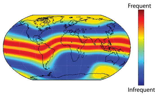
Worldwide Characteristics. Many studies have shown that scintillation activity varies with operating frequency, geographic location, local time, season, magnetic activity, and the 11-year solar cycle. FIGURE 1 shows a map indicating how scintillation activity varies with geographic location. The Earth’s magnetic field has a major influence on the occurrence of scintillation and regions of the globe with similar scintillation characteristics are aligned with the magnetic poles and associated magnetic equator. The regions located approximately 15° north and south of the magnetic equator (shown in red) are referred to as the equatorial anomaly. These regions experience the most significant activity including deep signal fades that can cause a GNSS receiver to briefly lose track of one or more satellite signals. Less intense fades are experienced near the magnetic equator (shown as a narrow yellow band in between the two red bands) and also in regions immediately to the north and south of the anomaly regions. Scintillation is more intense in the anomaly regions than at the magnetic equator because of a special situation that occurs in the equatorial ionosphere. The combination of electric and magnetic fields about the Earth cause free electrons to be lifted vertically and then diffuse northward and southward. This action reduces the ionization directly over the magnetic equator and increases the ionization over the anomaly regions. The word “anomaly” signifies that although the sun shines above the equator, the ionization attains its maximum density away from the equator.
FIGURE 1. Global occurrence characteristics of scintillation. (Figure courtesy of P. Kintner)
Low-latitude scintillation is seasonally dependent and is limited to local nighttime hours. The high-latitude region can also encounter significant signal fades. Here scintillation may also accompany the more familiar ionospheric effect of the aurora borealis (or aurora australis near the southern magnetic pole) and also localized regions of enhanced ionization referred to as polar patches. The occurrence of scintillation at auroral latitudes is strongly dependent on geomagnetic activity levels, but can occur in all seasons and is not limited to local nighttime hours. In the mid-latitude regions, scintillation activity is rare, occurring only in response to extreme levels of ionospheric storms. During these periods, the active aurora expands both poleward and equatorward, exposing the mid-latitude region to scintillation activity. In all regions, increased solar activity amplifies scintillation frequency and intensity. Scintillation effects are also a function of operating frequency, with lower signal frequencies experiencing more significant scintillation effects.
Scintillation Activity. Scintillation may accompany ionospheric behavior that causes changes in the measured range between the receiver and the satellite. Such delay effects are not discussed in detail here but are well covered in the literature and in a previous white paper by our group (see Further Reading, available online).
Amplitude scintillation can create deep signal fades that interfere with a user’s ability to receive GNSS signals. During scintillation, the ionosphere does not absorb the signal. Instead, irregularities in the index of refraction scatter the signal in random directions about the principal propagation direction. As the signal continues to propagate down to the ground, small changes in the distance of propagation along the scattered ray paths cause the signal to interfere with itself, alternately attenuating or reinforcing the signal measured by the user. The average received power is unchanged, as brief, deep fades are followed by longer, shallower enhancements.
Phase scintillation describes rapid fluctuations in the observed carrier phase obtained from the receiver’s phase lock loop. These same irregularities can cause increased phase noise, cycle slips, and even loss of lock if the phase fluctuations are too rapid for the receiver to track.
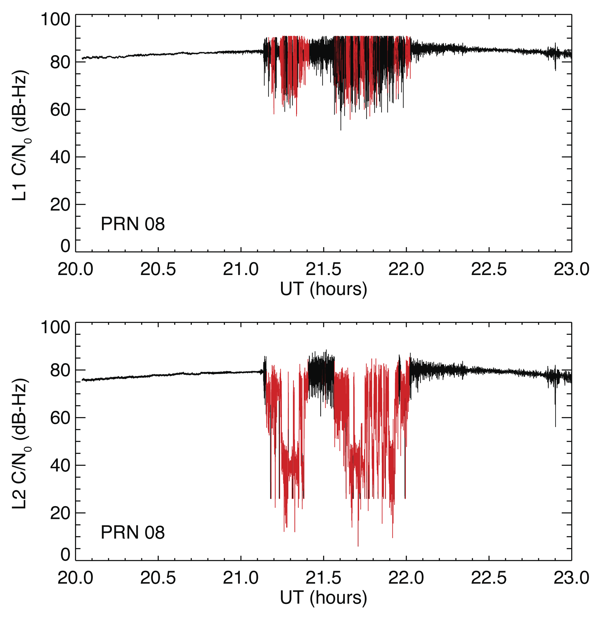
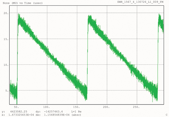
Equatorial and Low Latitude Scintillations. As illustrated in Figure 1, the regions of greatest concern are the equatorial anomaly regions. In these regions, scintillation can occur abruptly after sunset, with rapid and deep fading lasting up to several hours. As the night progresses, scintillation may become more sporadic with intervals of shallow fading. FIGURE 2 illustrates the scintillation effect with an example of intense fading of the L1 and L2 GPS signals observed in 2002, near a peak of solar activity. The observations were made at Ascension Island located in the South Atlantic Ocean under a region that has exhibited some of the most intense scintillation activity worldwide. The receiver that collected this data was one that employs a semi-codeless technique to track the L2 signal. Scintillation was observed on both the L1 and L2 frequencies with 20 dB fading on L1 and nearly 60 dB on L2 (the actual level of L2 fading is subject to uncertainty due to the limitations of semi-codeless tracking). This level of fading caused the receiver to lose lock on this signal multiple times. Signal fluctuations depicted in red indicate data samples that failed internal quality control checks and were thereby excluded from the receiver’s calculation of position. The dilution of precision (DOP), which is a measure of how pseudorange errors translate to user position errors, increased each time this occurred. In addition to the increase in DOP, elevated ranging errors are observed along the individual satellite links during scintillation.
FIGURE 2. Fading of the L1 and L2 Signals from one GPS satellite recorded from Ascension Island on March 16, 2002. Absolute power levels are arbitrary. (Figure courtesy of C. Carrano)
FIGURE 3 illustrates the relationship between amplitude and phase scintillations, also using measurements from Ascension Island. As shown in the figure, the most rapid phase changes are typically associated with the deepest signal fades (as the signal descends into the noise). Labeled on these plots are various statistics of the scintillating GPS signal: S4 is the scintillation intensity index that measures the relative magnitude of amplitude fluctuations, τI is the intensity decorrelation time, which characterizes the rate of signal fading, and σφ is the phase scintillation index, which measures the magnitude of carrier-phase fluctuations.
FIGURE 3. Intensity (top) and phase scintillations (bottom) of the GPS L1 signal recorded from Ascension Island on March 12, 2002. (Figure courtesy of C. Carrano)
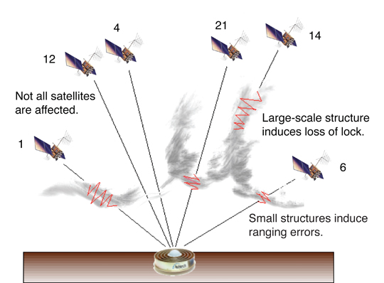
The ionospheric irregularities that cause scintillation vary greatly in spatial extent and drift with the background plasma at speeds of 50 to 150 meters per second. They are characterized by a patchy pattern as illustrated by the schematic shown in FIGURE 4. The patches of irregularities cause scintillation to start and stop several times per night, as the patches move through the ray paths of the individual GPS satellite signals. In the equatorial region, large-scale irregularity patches can be as large as several hundred kilometers in the east-west direction and many times that in the north-south direction. The large-scale irregularity patches contain small-scale irregularities, as small as 1 meter, which produce scintillation. Figure 4 is an illustration of how these structures can impact GNSS positioning. Large-scale structures, such as that shown traversed by the signal from PRN 14, can also cause significant variation in ionospheric delay and a loss of lock on a signal. Smaller structures, such as those shown traversed by PRNs 1, 21, and 6, are less likely to cause loss of the signal, but still can affect the integrity of the signal by producing ranging errors. Finally, due to the patchy nature of irregularity structures, PRNs 12 and 4 could remain unaffected as shown. Since GNSS navigation solutions require valid ranging measurements to at least four satellites, the loss of a sufficiently large number of satellite links has the potential to adversely affect system performance.
FIGURE 4. Schematic of the varying effects of scintillation on GPS.
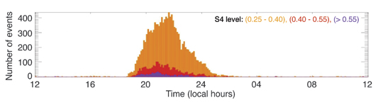
FIGURE 5 illustrates the local time variation of scintillations. As can be seen, GPS scintillations generally occur shortly after sunset and may persist until just after local midnight. After midnight, the level of ionization in the ionosphere is generally too low to support scintillation at GNSS frequencies. This plot has been obtained by cumulating, then averaging, all scintillation events at one location over one year corresponding to low solar activity. For a high solar activity year, the same local time behavior is expected, with a higher level of scintillations.
FIGURE 5. Local time distribution of scintillation events from June 2006 to July 2007 (in 6 minute intervals). (Figure courtesy of Y. Béniguel)
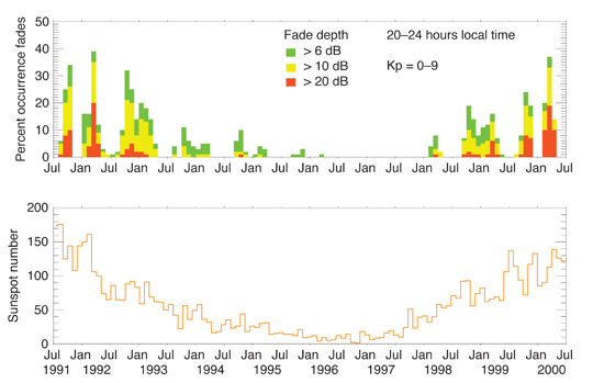
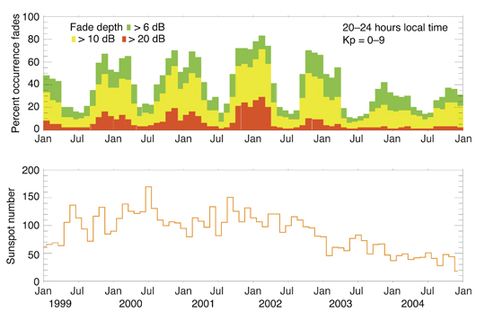
FIGURE 6 (top panel) shows the variation of the monthly occurrence of scintillation during the pre-midnight hours at Ascension Island. The scintillation data was acquired by the use of Inmarsat geostationary satellite transmissions at 1537 MHz (near the GNSS L1 band). The scintillation occurrence is illustrated for three levels of signal fading, namely, > 20 dB (red), > 10 dB (yellow), and > 6 dB (green). The bottom panel shows the monthly sunspot number, which correlates with solar activity and indicates that the study was performed during the years 1991 to 2000, extending from the peak of solar cycle 22 to the peak of solar cycle 23. Note that there is an increase in scintillation activity during the solar maximum periods, and there exists a consistent seasonal variation that shows the presence of scintillation in all seasons except the May-July period. This seasonal pattern is observed from South American longitudes through Africa to the Near East. Contrary to this, in the Pacific sector, scintillations are observed in all seasons except the November-January period. Since the frequency of 1537 MHz is close to the L1 frequencies of GPS and other GNSS including GLONASS and Galileo, we may use Figure 6 to anticipate the variation of GNSS scintillation as a function of season and solar cycle. Indeed, in the equatorial region during the upcoming solar maximum period in 2012-2013, we should expect GNSS receivers to experience signal fades exceeding 20 dB, twenty percent of the time between sunset and midnight during the equinoctial periods.
FIGURE 6. Frequency of occurrence of scintillation fading depths at Ascension Island versus season and solar activity levels. (Figure courtesy of P. Doherty)
High Latitude Scintillation. At high latitudes, the ionosphere is controlled by complex processes arising from the interaction of the Earth’s magnetic field with the solar wind and the interplanetary magnetic field. The central polar region (higher than 75° magnetic latitude) is surrounded by a ring of increased ionospheric activity called the auroral oval. At night, energetic particles, trapped by magnetic field lines, are precipitated into the auroral oval and irregularities of electron density are formed that cause scintillation of satellite signals. A limited region in the dayside oval, centered closely around the direction to the sun, often receives irregular ionization from mid-latitudes. As such, scintillation of satellite signals is also encountered in the dayside oval, near this region called the cusp.
When the interplanetary magnetic field is aligned oppositely to the Earth’s magnetic field, ionization from the mid-latitude ionosphere enters the polar cap through the cusp and polar cap patches of enhanced ionization are formed. The polar cap patches develop irregularities as they convect from the dayside cusp through the polar cap to the night-side oval. During local winter, there is no solar radiation to ionize the atmosphere over the polar cap but the convected ionization from the mid-latitudes forms the polar ionosphere. The structured polar cap patches can cause intense satellite scintillation at very high and ultra-high frequencies. However, the ionization density at high latitudes is less than that in the equatorial region and, as such, GPS receivers, for example, encounter only about 10 dB scintillations in contrast to 20-30 dB scintillations in the equatorial region.
FIGURE 7 shows the seasonal and solar cycle variation of 244-MHz scintillations in the central polar cap at Thule, Greenland. The data was recorded from a satellite that could be viewed at high elevation angles from Thule. It shows that scintillation increases during the solar maximum period and that there is a consistent seasonal variation with minimum activity during the local summer when the presence of solar radiation for about 24 hours per day smoothes out the irregularities.
FIGURE 7. Variation of 244-MHz scintillations at Thule, Greenland with season and solar cycle. (Figure courtesy of P. Doherty)
The irregularities move at speeds up to ten times larger in the polar regions as compared to the equatorial region. This means that larger sized structures in the polar ionosphere can create phase scintillation and that the magnitude of the phase scintillation can be much stronger. Large and rapid phase variations at high latitudes will cause a Doppler frequency shift in the GNSS signals which may exceed the phase lock loop bandwidth, resulting in a loss of lock and an outage in GNSS receivers.
As an example, on the night of November 7–8, 2004, there was a very large auroral event, known as a substorm. This event resulted in very bright aurora and, coincident with a particularly intense auroral arc, there were several disruptions to GPS monitoring over the region of Northern Scandinavia. In addition to intermittent losses of lock on several GPS receivers and to phase scintillation, there was a significant amplitude scintillation event. This event has been shown to be very closely associated with particle ionization at around 100 kilometers altitude during an auroral arc event. While it is known that substorms are common events, further studies are still required to see whether other similar events are problematic for GNSS operations at high latitudes.
Scintillation Effects
We had mentioned earlier that the mid-latitude ionosphere is normally benign. However, during intense magnetic storms, the mid-latitude ionosphere can be strongly disturbed and satellite communication and GNSS navigation systems operating in this region can be very stressed. During such events, the auroral oval will extend towards the equator and the anomaly regions may extend towards the poles, extending the scintillation phenomena more typically associated with those regions into mid-latitudes.
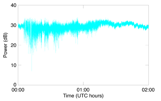
An example of intense GPS scintillations measured at mid-latitudes (New York) is shown in FIGURE 8. This event was associated with the intense magnetic storm observed on September 26, 2001, during which the auroral region had expanded equatorward to encompass much of the continental U.S. This level of signal fading was sufficient to cause loss of lock on the L1 signal, which is relatively rare. The L2 signal can be much more susceptible to disruption due to scintillation during intense storms, both because the scintillation itself is stronger at lower frequencies and also because semi-codeless tracking techniques are less robust than direct correlation as previously mentioned.
FIGURE 8. GPS scintillations observed at a mid-latitude location between 00:00 and 02:00 UT during the intense magnetic storm of September 26, 2001. (Figure courtesy of B. Ledvina)
Effects of Scintillation on GNSS and SBAS
Ionospheric scintillation affects users of GNSS in three important ways: it can degrade the quantity and quality of the user measurements; it can degrade the quantity and quality of reference station measurements; and, in the case of SBAS, it can disrupt the communication from SBAS GEOs to user receivers. As already discussed, scintillation can briefly prevent signals from being received, disrupt continuous tracking of these signals, or worsen the quality of the measurements by increasing noise and/or causing rapid phase variations. Further, it can interfere with the reception of data from the satellites, potentially leading to loss of use of the signals for extended periods. The net effect is that the system and the user may have fewer measurements, and those that remain may have larger errors. The influence of these effects depends upon the severity of the scintillation, how many components are affected, and how many remain.
Effect on User Receivers. Ionospheric scintillation can lead to loss of the GPS signals or increased noise on the remaining ones. Typically, the fade of the signal is for much less than one second, but it may take several seconds afterwards before the receiver resumes tracking and using the signal in its position estimate. Outages also affect the receiver’s ability to smooth the range measurements to reduce noise. Using the carrier-phase measurements to smooth the code substantially reduces any noise introduced. When this smoothing is interrupted due to loss of lock caused by scintillation, or is performed with scintillating carrier-phase measurements, the range measurement error due to local multipath and thermal noise could be from three to 10 times larger. Additionally, scintillation adds high frequency fluctuations to the phase measurements further hampering noise reduction.
Most often scintillation will only affect one or two satellites causing occasional outages and some increase in noise. If many well-distributed signals are available to the user, then the loss of one or two will not significantly affect the user’s overall performance and operations can continue. If the user has poor satellite coverage at the outset, then even modest scintillation levels may cause an interruption to their operation. When scintillation is very strong, then many satellites could be affected significantly. Even if the user has excellent satellite coverage, severe scintillation could interrupt service. Severe amplitude scintillation is rarely encountered outside of equatorial regions, although phase effects can be sufficiently severe at high latitudes to cause widespread losses of lock.
Effect on Reference Stations. The SBAS reference stations consist of redundant GPS receivers at precisely surveyed locations. SBAS receivers need to track two frequencies in order to separate out ionospheric effects from other error sources. Currently these receivers use the GPS L1 C/A-code signal and apply semi-codeless techniques to track the L2 P(Y) signal. Semi-codeless tracking is not as robust as either L1 C/A or future civil L5 tracking. The L2 tracking loops require a much narrower bandwidth and are heavily aided with scaled-phase information from the L1 C/A tracking loops. The net effect is that L2 tracking is much more vulnerable to phase scintillation than L1 C/A, although, because of the very narrow bandwidth, L2 tracking may be less susceptible to amplitude scintillation. Because weaker phase scintillation is more common than stronger amplitude scintillation, the L2 signal will be lost more often than L1. The SBAS reference stations must have both L1 and L2 measurements in order to generate the corrections and confidence levels that are broadcast. Severe scintillation affecting a reference station could effectively prevent several, or even all, of its measurements from contributing to the overall generation of corrections and confidences. Access to the L5 signal will reduce this vulnerability. The codes are fully available, the signal structure design is more robust, and the broadcast power is increased. L5-capable receivers will suffer fewer outages than the current L2 semi-codeless ones, however strong amplitude scintillation will still cause disruptions. Strong phase scintillation may as well.
If scintillation only affects a few satellites at a single reference station, the net impact on user performance will likely be small and regional. However, if multiple reference stations are affected by scintillation simultaneously, there could be significant and widespread impact.
Effect on Satellite Datalinks. The satellites not only provide ranging information, but also data. When scintillation causes the loss of a signal it also can cause the loss or corruption of the data bits.
Each GPS satellite broadcasts its own ephemeris information, so the loss of data on an individual satellite affects only that satellite. A greater concern is the SBAS data transmissions on GEOs. This data stream contains required information for all satellites in view including required integrity information. If the data is corrupted, all signals may be affected and loss of positioning becomes much more likely.
Mitigation Techniques. There are several actions that SBAS service providers can take to lessen the impact of scintillation. Increasing the margin of performance is chief among them. The more satellites a user has before the onset of scintillations, the more likely he will retain performance during a scintillation event. In addition, having more satellites means that a user can tolerate more noise on their measurements. Therefore, incorporating as many satellites as possible is an effective means of mitigation. GNSS constellations in addition to GPS are being developed. Including their signals into the user position solution would extend the sky coverage and improve the performance under scintillation conditions. (See the white paper for other mitigation techniques.)
Conclusions and Further Work
Ionospheric scintillations are by now a well-known phenomenon in the GNSS user community. In equatorial regions, ionospheric scintillations are a daily feature during solar maximum years. In auroral regions, ionospheric scintillations are not strongly linked to time of the day. In the mid-latitude regions, scintillations tend to be linked to ionospheric disturbances where strong total electron content gradients can be observed (ionospheric storms, strong traveling ionospheric disturbances, solar eclipses, and so on).
While the global climatic models of ionospheric scintillations can be considered satisfactory for predicting (on a statistical basis) the occurrence and intensity of scintillations, the validation of these models is suffering from the fact that at very intense levels of scintillation, even specially designed scintillation receivers are losing lock. Also, the development of models that can predict reliably the size of scintillation cells (regions of equal scintillation intensity), which allows establishing joint probabilities of losing more than one satellite simultaneously, is still ongoing.
The data presented in Figure 2 was produced by an Ashtech, now Ashtech S.A.S. Z-XII GPS receiver. The data presented in Figure 5 was obtained from Javad, now Javad GNSS and Topcon Legacy GPS receivers and GPS Silicon Valley, now NovAtel GSV4004 GPS scintillation receivers. The data presented in Figure 8 was obtained from a non-commercial receiver.
The Satellite-Based Augmentation Systems Ionospheric Working Group was formed in 1999 by scientists and engineers involved with the development of the Satellite Based Augmentation Systems in an effort to better understand the effects of the ionosphere on the systems and to identify mitigation strategies. The group now consists of over 40 members worldwide.
The scintillation white paper was principally developed by Bertram Arbesser-Rastburg, Yannick Béniguel, Charles Carrano, Patricia Doherty, Bakry El-Arini, and Todd Walter with the assistance of other members of the working group.
“Morphology of Phase and Intensity Scintillations in the Auroral Oval and Polar Cap” by S. Basu, S. Basu, E. MacKenzie, and H. E. Whitney in Radio Science, Vol. 20, No. 3, May–June 1985, pp. 347–356, doi: 10.1029/RS020i003p00347.
“Global Morphology of Ionospheric Scintillations” by J. Aarons in Proceedings of the IEEE, Vol. 70, No. 4, April 1982, pp. 360–378, doi: 10.1109/PROC.1982.12314.
“Equatorial Scintillation – A Review” by S. Basu and S. Basu in Journal of Atmospheric and Terrestrial Physics, Vol. 43, No. 5/6, pp. 473–489, 1981, doi: 10.1016/0021-9169(81)90110-0.
• Effects of Scintillations on GNSS
“GNSS and Ionospheric Scintillation: How to Survive the Next Solar Maximum by P. Kintner, Jr., T. Humphreys, and J. Hinks in Inside GNSS, Vol. 4, No. 4, July/August 2009, pp. 22–30.
“Analysis of Scintillation Recorded During the PRIS Measurement Campaign” by Y. Béniguel, J.-P. Adam, N. Jakowski, T. Noack, V. Wilken, J.-J. Valette, M. Cueto, A. Bourdillon, P. Lassudrie-Duchesne, and B. Arbesser-Rastburg in Radio Science, Vol. 44, RS0A30, 11 pp., 2009, doi:10.1029/2008RS004090.
“Characteristics of Deep GPS Signal Fading Due to Ionospheric Scintillation for Aviation Receiver Design” by J. Seo, T. Walter, T.-Y. Chiou, and P. Enge in Radio Science, Vol. 44, RS0A16, 2009, doi: 10.1029/2008RS004077.
“GPS and Ionospheric Scintillations” by P. Kintner, B. Ledvina, and E. de Paula in Space Weather, Vol. 5, S09003, 2007, doi: 10.1029/2006SW000260.
“Space Weather Effects of October–November 2003” by P. Doherty, A. Coster, and W. Murtagh in GPS Solutions, Vol. 8, No. 4, pp. 267–271, 2004, doi: 10.1007/s10291-004-0109-3.
“First Observations of Intense GPS L1 Amplitude Scintillations at Midlatitude” by B. Ledvina, J. Makela, and P. Kintner in Geophysical Research Letters, Vol. 29, No. 14, 1659, 2002, doi: 10.1029/2002GL014770.
• Previous “Innovation” Articles on Space Weather and GNSS
When jamming interfered with GPS signals at Newark Airport, a three-month effort determined that low-power, mobile personal-privacy devices were responsible. This article describes how they were found and outlines how the observable parameters of such devices encompass a wide variation in RF spectra and internal modulation.
Personal privacy devices (PPDs) are now recognized as being responsible for causing interference to GPS receivers. However, in November of 2009, when the Local-Area Augmentation System (LAAS) installed its first Ground-Based Augmentation System (GBAS) at Newark International Airport (EWR), this fact was not known. Within the first month of its installation, anomalies in GBAS processing were correlated to the presence of radio-frequency interference (RFI). Initial efforts to determine the source of this unexpected RFI were not successful.
The Federal Aviation Administration (FAA) had a significant interest in finding this RFI source, leading to deployment of RFI detection and location equipment by several groups. Zeta Associates temporarily installed equipment in early January 2010 that was capable of detecting and characterizing RFI but did not have emitter location capability.
Determining that an RFI transmitter is in motion is more certain if the RFI is observed simultaneously by multiple sensors. However, analysis from hundreds of RFI events indicates that when an RFI source is in motion, observations collected by a single sensor can provide sufficient information to determine that the RFI transmitter is in motion.
Continuing interest in understanding PPD effects on GPS receivers led to the installation of remotely accessible monitoring equipment that provides detailed characteristics of these devices. Remote access facilitates monitoring, particularly since PPDs are present for 30 to 60 seconds at a time and only a few times a day.
Background
The January 2010 deployment included a WAAS GPS receiver, spectrum analyzer, and a Zeta custom-developed Snapshot System, assembled from commercial off-the-shelf (COTS) equipment for conducting WAAS site-installation surveys, and capable of capturing intermittent short-duration RFI events. It consists of a tuneable receiver (10 MHz to 3 GHz) whose RF front end spans 25 MHz that is digitized at a sample rate of 56 MHz, with storage capacity sufficient for up to 80 minutes. Once captured, the time-series data can be analyzed in many different ways. Possible analysis techniques include examination of the raw time samples, generation of spectral plots, or demodulation of the RFI signal. Each approach can lead to a better understanding of the underlying interference signal. If digital data is present and can be demodulated, it might be possible to associate the demodulated bits with a known transmitter.
Data can be captured manually or programmatically using a trigger determined by an algorithm that monitors WAAS GPS receiver automatic gain control (AGC) logs. The AGC function within a WAAS receiver has a well-behaved response for normal Gaussian noise RF environments. When RFI is present, the AGC exhibits atypical responses that then trigger the Snapshot System. As WAAS receivers utilize both L1 and L2, and each RF path has its own AGC, it is possible to detect the presence of potential RFI at either L1 or L2.
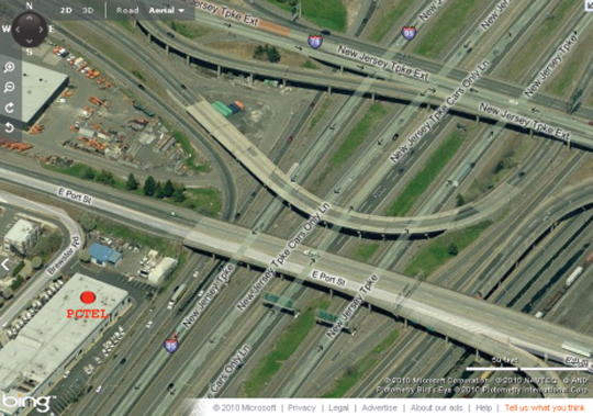
The Snapshot System RF input for this deployment was from a PCTEL antenna identical to those used at WAAS reference sites. This antenna incorporates a triplexer that provides three separate 40 MHz passbands each centered on L1, L2, and L5, with approximately 50 dB of gain. This antenna was located approximately one mile north of the four LAAS antennas within Port Authority of New York and New Jersey (PANYNJ) Building 80.
Within the first hour of being deployed on January 20, 2010 the Snapshot System had detected and captured one RFI event in the GPS L1 band. After one day, the Snapshot System had detected and captured more than 25 separate instances of RFI within the GPS L1 band. Most RFI events were narrowband (10s of kHz bandwidth) and short duration (no more than 3 seconds).
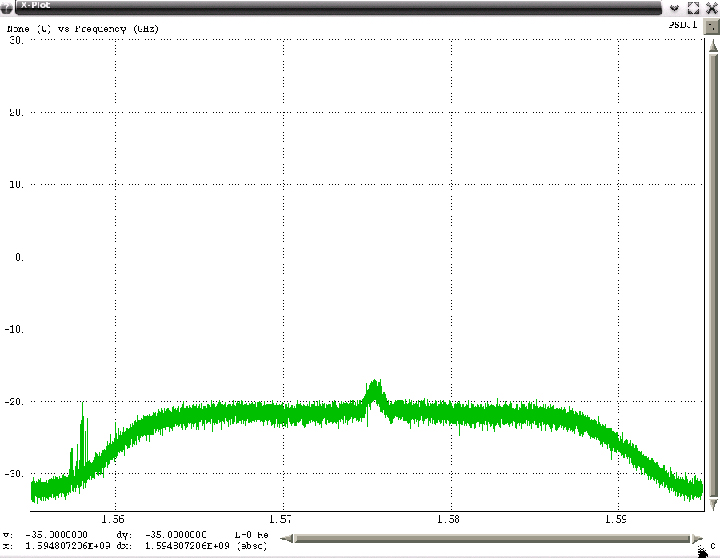
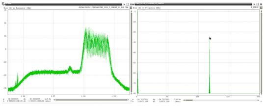
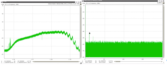
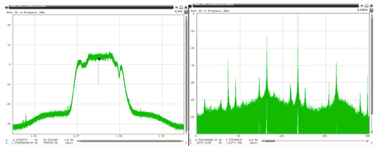
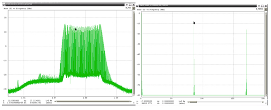
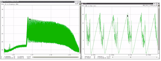
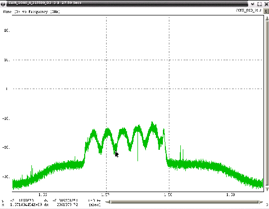
However, there also were five RFI events that spanned more than 15 MHz across L1 (Figure 1) were present as long as 20 seconds and at a power level as much as 25 dB above the receive antenna’s noise floor. Some of these RFI events were strong enough to reduce a WAAS G-II receiver C/N0 by as much as 20 dB and thereby resulted in loss of tracking for lower-elevation GPS satellites. Higher-elevation GPS satellites were able to continue tracking throughout these events but at a lower C/N0. The wideband RFI events were also detected by the SLS 4000 GBAS monitor and coincided with tracking problems in the LAAS GBAS receivers.
FIGURE 1. EWR wideband RFI.
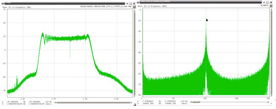
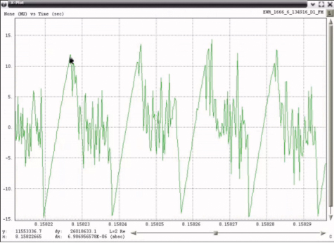
Two of the captured broadband RFI events were demodulated and analyzed. The underlying linear frequency modulation (FM) signal swept over more than 15 MHz in less than 1 millisecond (Figure 2).
FIGURE 2. FM demodulated wideband RFI.
At that time, it was not known if the source of the RFI was stationary or moving, whether it was unintentional (emanating from a licensed transmitter but with malfunctioning electronics), inadvertent (equipment normally used for test purposes and capable of operating in the GPS band but accidentally left on), or intentional (purposeful jamming of GPS).
Since the RFI was observed by GPS receivers separated by 1,700 meters, a search was undertaken to identify any other GPS receivers in the vicinity of EWR. One National Geodetic Survey (NGS) continuously operating reference site (CORS) NJI2 is located near EWR about 4,500 meters northwest from Building 80. Analysis of data from NJI2 during the same time periods that RFI was detected by the WAAS and LAAS receivers did not contain any indication of RFI, and therefore suggested that the source of RFI was more localized to EWR.
The Snapshot System remained in place for approximately two weeks before moving to another location. Collected data was analyzed, showing that wideband RFI was associated with significant degradation to both the WAAS and LAAS receivers. Additional characteristics noted the RFI was intermittent, lasting typically 30 seconds but no more than 60 seconds, was observed more often Monday through Friday, and most frequently around 8 a.m. local time.
Locating The RFI
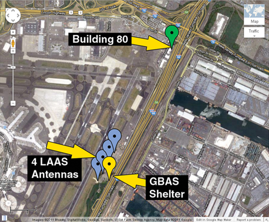
Figure 3 shows a Google map of EWR with blue dots indicating the location of the four LAAS antennas, a green dot for Building 80, and a yellow dot for the GBAS shelter. EWR is adjacent to the New Jersey Turnpike (NJT), which has seven southbound and seven northbound lanes of traffic.
FIGURE 3 Google map of EWR.
Since the Snaphsot System did not include location capability, other teams with direction-finding equipment, including beam-forming antennas, travelled to EWR to try to locate the RFI source. These teams were on site at various times from February to March. However, those efforts did not provide sufficiently reliable information to reduce the search area. By mid-March, the search area remained identical to that of January.
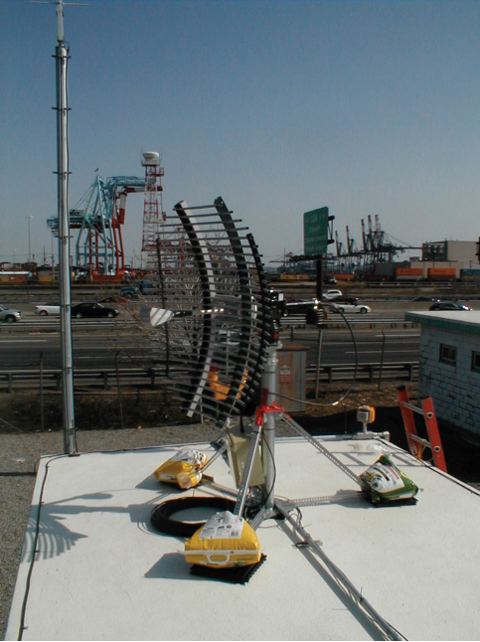
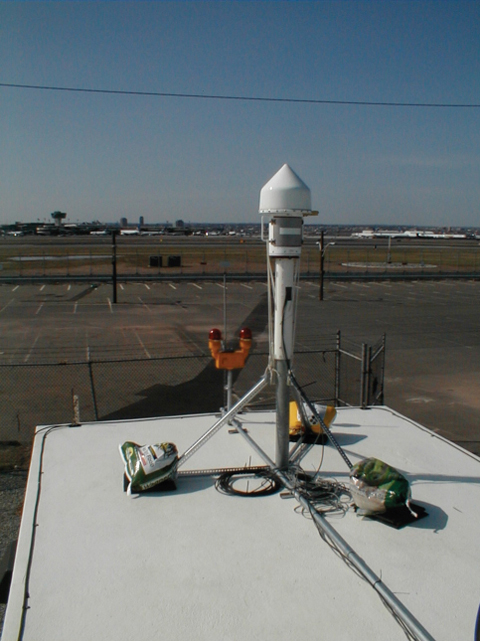
Zeta then deployed two WAAS G-II receivers separated by considerable distance (1,722 meters) to monitor for RFI, and analyze each receiver’s response only when RFI sufficient to significantly degrade GPS reception was detected. One receiver was located within Building 80, and the second receiver within the GBAS shelter near the LAAS antennas. This configuration was designed to determine degradation relative to each reference receiver and thereby establish probable search areas for the RFI emitter. The Zeta equipment also incorporated a rotating directional antenna (at the GBAS shelter shown in Figure 4) that was commanded to rotate only when significant RFI was detected.
FIGURE 4A. Antennas on roof of GBAS shelter.FIGURE 4B. Antennas on roof of GBAS shelter.
The expectation was that RFI would be detected simultaneously by both GPS receivers, and that the relative degradation in normalized C/ N0 would provide an indication as to which location lay in closer proximity to the RFI source. The rotating high-gain directional antenna would then indicate a reduced probable search area consistent with the relative degradation between the two receivers. At the time this equipment was deployed, it was still thought that the RFI was most likely stationary and high-power. However, the measurement results were quite different than expected. Subsequent data analysis from this equipment revealed that the RFI was low-power and moving, specifically moving along the NJT.
The Zeta equipment was deployed on March 19, 2010, and remained in place while operating automatically. On March 25, data collected during the previous week were analyzed. During this 1-week collection there were 11 instances when both receivers detected wideband RFI events and one antenna rotation even partially tracked one wideband RFI emitter. Such data was indicative of a non-stationary emitter, a finding that was quite significant. Based on data from the two receivers, the apparent velocity of the RFI emitters ranged between 45 miles per hour (mph) to 72 mph. Initial analysis of antenna-rotation data also indicated the RFI source was east of the GBAS shelter and moving south on the NJT.
Understanding the importance of degradations from both receivers was crucial in determining that the RFI has attributes of transmitting at low power and is moving. Had a single stationary RFI emitter been responsible for these observations, the degradations measured at each receiver would have occurred at essentially the same time, not 50 to 80 seconds apart. A high-power moving RFI emitter would also have produced degradations at both receivers at the same time, and since that was not observed, the conclusion was that the RFI emitter was relatively low in output power. Low-power RFI emitters will cause significant degradation to GPS receivers only when they are in close proximity to them, on the order of hundreds of meters.
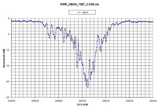
Receiver data logs were processed specifically for degradation in normalized C/N0. Normalized C/N0 was only computed for those satellites above 20 degrees, and all of those results were averaged together. Prior knowledge regarding WAAS PCTEL antennas has established an expected C/N0 versus satellite elevation that is accurate to approximately ±1 dB with a nominal mean of 0 dB. This normalized C/N0 represents an average of all satellites in view. However, individual satellite signal strength can vary greater than ± 1 dB. Significant deviations of more than –3 dB are indicative of strong RFI within the GPS processing band. Normalized C/N0 was plotted for each day that data was collected, followed by expanding those time periods where significant degradation was present.
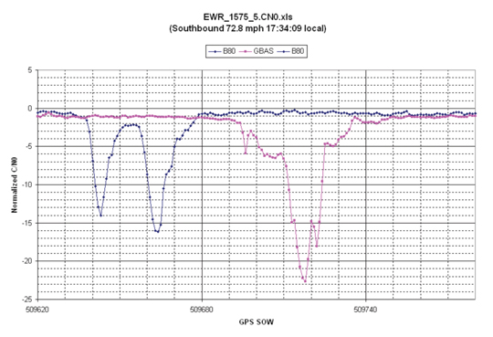
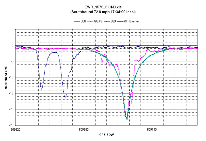
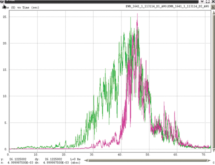
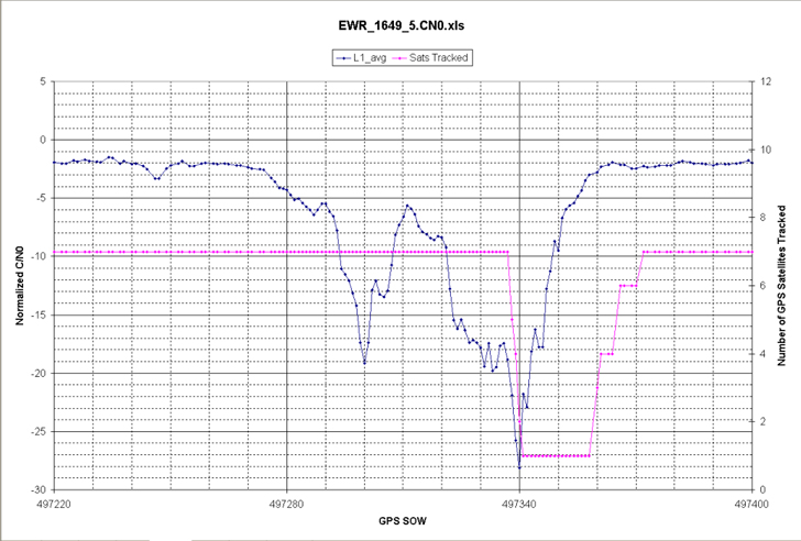
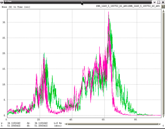
Figure 5 shows data of the first evidence of a low-power moving PPD. Data for Building 80 receiver is in blue and data from the GBAS shelter receiver in pink. Since Building 80 is north of the GBAS shelter, when degradations occurred first at Building 80, this implies that the RFI emitter is moving from north to south. Similarly, when degradations were first seen at the GBAS shelter, the RFI emitter was moving from south to north. This plot uses major time grids of 60 seconds and minor grids of 10 seconds.
FIGURE 5. Normalized C/N0 observed at Building 80 and GBAS shelter.
The double separate degradations observed by the Building 80 receiver have only been observed from monitoring equipment located at that building, and have since been associated with travel paths of PPDs on the nearby highways. Both GPS receiver and spectral data contain this same characteristic. This characteristic is due to the fact that vehicles traveling south on the NJT have clear line of sight to the roof of Building 80 (shown by Figure 6) before they travel under Interstate 78, after which they pass next to Building 80. During the time that they are under Interstate 78, their transmissions are blocked in the direction of the roof of Building 80.
FIGURE 6A. View of NJT near Building 80.FIGURE 6B. View of NJT near Building 80.
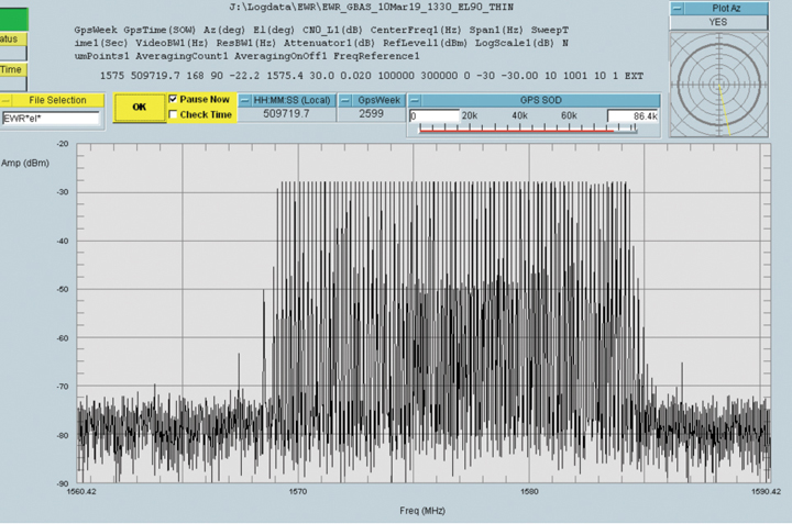
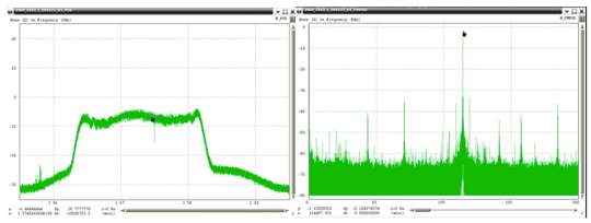
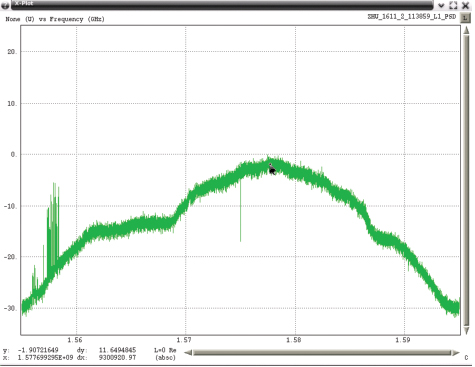
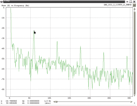
Spectral data as observed by the 4-foot reflector is shown in Figure 7. Figure 8 shows spectral maximum data as collected by the 4-foot linearly polarized reflector along with additional information.
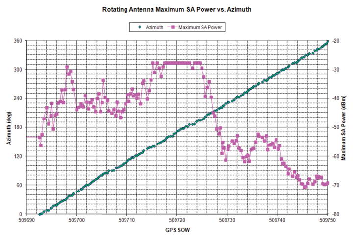
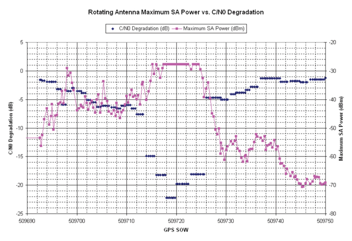
FIGURE 7. Wideband RFI observed by 4-foot reflector (click to enlarge.)FIGURE 8A. Pink represents spectral maximum data as observed through the reflector, green represents the azimuth of that antenna, and blue the reported degradation of the GBAS shelter receiver.FIGURE 8B. Pink represents spectral maximum data as observed through the reflector, green represents the azimuth of that antenna, and blue the reported degradation of the GBAS shelter receiver.
When the GBAS shelter receiver at first detected RFI, the reflector began rotating from an azimuth of 0 degrees in a clockwise direction. At the same time, a spectrum analyzer began capturing spectra at a rate of 3 per second. The first spectral maximum was observed at an azimuth of 30 degrees, a direction in which the antenna was pointed towards the NJT, to a location approximately 900 meters away from the GBAS shelter. The next time spectra were at high levels occurred for azimuths between 145 to 195 degrees, or southeast of the GBAS shelter. The approach of using a rotating antenna was originally intended to provide a direction towards a stationary source and not to track a moving emitter. However, it appears that to some extent, the rotating antenna in fact did track a moving emitter from north to south.
On the afternoon of the day these results were communicated to the FAA lead for the EWR RFI investigation, all search activities were shifted to the NJT and away from the airport operating area. Just south of the GBAS shelter there is an official-use overpass that straddles the NJT. All detection equipment was positioned onto the overpass, under the hypothesis that the RFI was emanating from vehicles traveling the NJT. Evidence substantiating this initial finding was found within a day, and approximately one month later a concerted effort was undertaken to identify and stop a single vehicle that was using a PPD.
The Zeta equipment remained in place for many months and continued to provide additional evidence of PPD characteristics. Early in the investigation it was hoped that only a few PPDs had been responsible, but as more data was collected it became evident that many different types of PPDs were traveling along the NJT past EWR.
Modeling PPD Effect
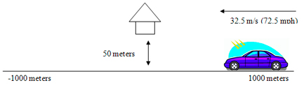
Once it was realized that the RFI was from low power moving emitters, a simple model was used to predict their degradation effect on WAAS GPS receivers. The model shown in Figure 9 was used for the purpose of computing distance between the RFI emitter and a WAAS antenna and to then compute the additional level of interference noise power that the WAAS antenna would receive. Here, the WAAS PCTEL antenna is located 50 meters from a road that is 2000 meters long and straight and has an RFI emitter transmitting +25 dBm, moving at 32.5 meters per second (72.5 mph) and with clear line of sight to the WAAS antenna.
FIGURE 9. Simple model of moving emitter.FIGURE 10. Model of normalized C/No due to a PPD.
With these assumptions it is a simple matter to compute the additional noise power at the WAAS antenna. Non-coherent summation of the RFI noise and inherent system noise was used to compute the total noise power and therefore the additional degradation in C/N0. The resulting predicted degradation was overlaid on one of the actual RFI events and is shown as a green line in Figure 10. The predicted degradation closely resembles actual event data logged by receivers.
The shape of degradation in normalized C/N0 versus time has been observed in nearly all of the EWR RFI events that have been analyzed. The magnitude of degradation depends on the power of the RFI and its proximity to the GPS antenna, while its time duration depends on the velocity of the vehicle carrying the PPD. The shape is directly related to the distance versus time between the vehicle and the WAAS antenna. Faster/slower moving vehicles with PPDs will simply shrink/stretch the time scale. Curved roadways would have different shapes that could also be readily predicted.
CORS data was revisited after realizing that PPDs were traveling the NJT. Specifically, two CORS sites CTDA (70 meters from Interstate 95) and NJDY (380 meters from Interstate 95) were identified. Data from those two sites were analyzed for a couple of weekdays. Possible evidence of PPDs was found within that data. Reported Signal to Noise Ratio (SNR) from CTDA and NJDY contained variations similar to those observed by GPS receivers at EWR during times when PPD induced RFI has been detected.
Continued RFI Monitoring
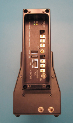
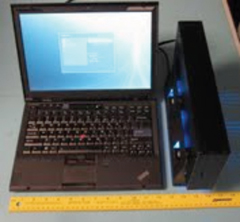
The LAAS program desired continued monitoring of RFI from PPDs near EWR, including estimates of their effective isotropic radiated power (EIRP). Additional equipment was assembled to provide this capability and installed on March 3, 2011. This monitoring equipment is located within the GBAS shelter at EWR and comprises several COTS components that incorporate improvements beyond the first Snapshot System used at EWR. Improvements include an upgraded Snapshot System (Figure 11), an RHCP directional antenna, and a wireless modem that provides remote access to the monitoring equipment.
Figure 11A. Snapshot System ICEPOD6-M5.FIGURE 11B. Snapshot System laptop.
Remote access makes it possible to analyze captured RFI data from any computer connected to the Internet, and to modify software if necessary. The new equipment configuration, specifically the use of an AEL AST 1507AA RHCP antenna, was chosen with the explicit purpose of establishing more accuracy in estimated EIRP.
Analysis of data collected during 2010 indicated three significant sources of error in estimating EIRP; Free Space Loss (FSL) from not knowing the exact position of the PPD on the NJT, polarization mismatch loss between the PPD antenna and the receive antenna, and the effects due to transmission from within a vehicle. Differences in FSL loss between the closest southbound lane on the NJT and the most distant northbound lane is on the order of 11 dB. If it is known that the PPD is traveling south, the difference in FSL between the nearest to farthest southbound lanes is less but still about 6 dB. FSL differences for northbound lanes are smaller, on the order of 3 dB. Knowing the direction of travel reduces this uncertainty but does not eliminate it. The WAAS PCTEL antenna is RHCP, but at the horizon has an axial ratio of approximately 5 dB. Many PPDs appear to be using quarter wavelength dipole antenna that are mounted with a rotatable connector. Assuming all PPD antennas are linearly polarized, there would then be an uncertainty of about 5 dB when using data observed by the WAAS PCTEL antenna. The AEL antenna has an axial ratio of 0.2 dB at L1 and significantly reduces uncertainty of polarization mismatch loss. Even though the AEL antenna has a 3 dB mismatch loss, that loss has an uncertainty of 0.2 dB for any orientation of the PPD antenna. The PCTEL antenna has a symmetric gain response relative to the NJT. The AEL antenna was pointed to the north intentionally so that observed RFI power will be stronger when a PPD is north of the GBAS shelter. Simultaneous capture of real time samples from both antennas by the ICEPOD6-M5 provides an indication of the direction in which the PPD is traveling. The third uncertainty comes from the effects of the PPD being located within a vehicle. Vehicular effects on the PPD transmitters were not accounted for due to difficulty in using a simple model. Aloi [1] has measured vehicular effects of quarter wavelength dipole antenna (typically used by PPDs) and has previously published [1] [2] on the effect of vehicles on GPS signals. His most recent findings have not yet been published but indicate that the type of vehicle, the location of a dipole antenna within it, and the position outside of the vehicle from which power is being measured, can lead to significant variation (10 to 15 dB) of the observable power. Consequently, the reported EIRP estimates from the Snapshot System have been referenced to a point just outside the vehicle and do not attempt to account for vehicular effects.
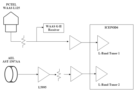
Figure 12 shows a block diagram of the current monitoring equipment. The PCTEL antenna along with the WAAS G-II receiver is used for monitoring GPS signals. WAAS G-II receiver logs are monitored continuously and saved to disk, but snapshots are only taken if the RFI algorithms indicate that RFI is present. A snapshot will be taken if any of three tests (based on AGC, normalized C/N0, or spectral power) are exceeded. Narrowband RFI tends to most impact the AGC response, while wideband RFI tends to trigger the normalized C/N0 metric. Since the Snapshot System is also continuously monitoring the RF spectra from both antennas, an additional test checks if there are significant spectra changes.
FIGURE 12. Current Snapshot monitoring block diagram.
The AEL antenna is connected to a filter/low noise amplifier (LNA) (Delta Microwave L5995) identical to those within the PCTEL antenna, before it is connected to one of the two L-band tuners (900 to 2200 MHz) of the ICE-Online ICEPOD6-M5, which includes 1 TB of long-term storage and 8 GB of high-speed RAM and is capable of sustained data transfers of as high as 400 MB/s between the L-band tuners and disk. Sample rates and RF filtering are programmable and have been set to use a complex sample rate of 40 MSPS and an RF bandwidth of 30 MHz. When RFI is present, data transfers are 320 MB/s. The internal 1 TB disk can store approximately 100 minutes of RFI. Software parameters limit RFI data capture for any single event to no more than 90 seconds. Implementation of a circular buffer within the high-speed RAM (8 seconds for each L-band tuner path) allows continuous capture of RF data while waiting for a trigger indicating that RFI is present. To reduce false alarms, RFI must be present for at least 4 seconds before data is captured. However, no RFI data is lost, because the circular buffer is longer than 4 seconds. RFI data captures typically contain 3 seconds of data at the beginning, with no RFI, and therefore make it possible to observe the onset of the RFI.
The new equipment has captured hundreds of RFI events, spanning a wide range in bandwidth (7 MHz to an estimated 150 MHz), chirp rate (9 kHz to 170 kHz), and power levels (–10 dBm to as much as +20 dBm). Accurately estimating EIRP of moving emitters is a challenge and requires detailed knowledge of the characteristics of all components used in generating the estimate. Furthermore, distance to the RFI source can only be inferred, since its movement precludes exact measurement, and consequently there will always be some uncertainty in any reported EIRP. However, even with these qualifications, there is evidence from Snapshot System data that some of the RFI sources are transmitting at power levels as much as +20 dBm.
Modeling Antenna Responses
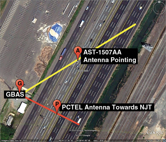
The use and orientation of the two antennas was chosen to determine the direction that PPDs are traveling and thereby reduce some of the uncertainty with respect to their exact location. Figure 13 shows the direction (58 degrees) in which the AEL antenna is pointed.
FIGURE 13. Pointing direction of the AEL antenna.
The combination of its beam width (70 degrees) and axial ratio (0.2 dB) results in a nearly uniform gain across all lanes north of the GBAS shelter. Although FSL still depends on the exact location of the PPD, this approach does reduce many of the uncertainties associated with estimating EIRP. Since the PCTEL antenna has an omnidirectional pattern it will have a symmetrical response.
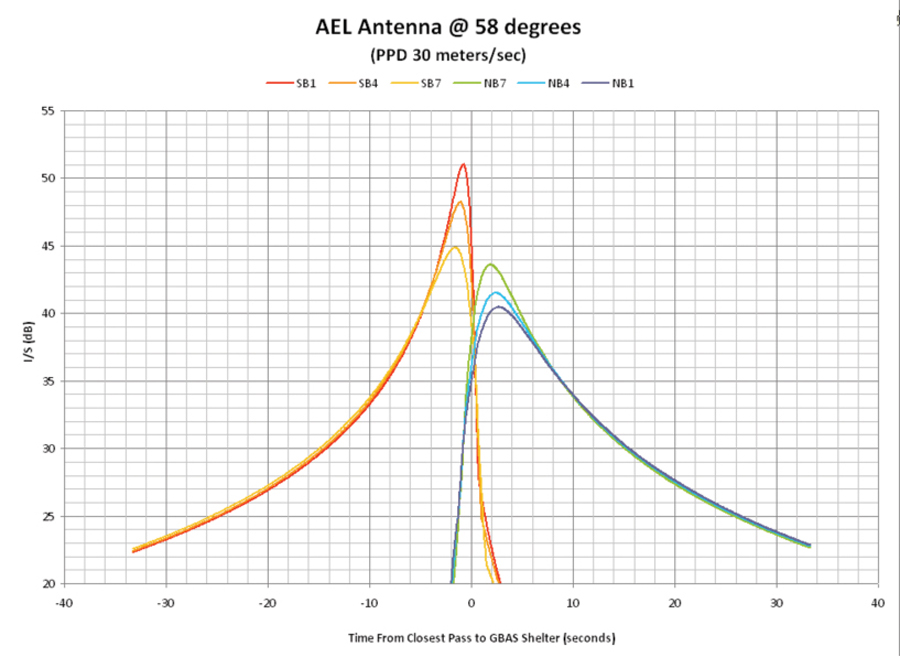
To determine the time that maximum PPD power would be observed by each antenna, a model was used that assumed the PPD was transmitting at constant power, with fixed polarization, travelling at a constant velocity, and there were no obstacles between the transmitter and each antenna. FSL was calculated for each second of travel and used to determine the magnitude of RFI power that would be received. This value was then used to calculate a nominal Interference to Signal (I/S) relative to the GPS signal. The distance between each antenna and each of the travel lanes on the NJT were also used. The intent of this model was to understand how I/S would vary with time for each of the NJT travel lanes. Figure 14 shows the predicted I/S for the PCTEL antenna and Figure 15 for the AEL antenna. In each of these plots red, yellow and orange represent 3 of the 7 south bound travel lanes and green, blue and purple represent 3 of the 7 north bound travel lanes. A time of 0 was used for the time when the PPD is nearest physically to the GBAS shelter. A nominal velocity of 30 meters/second (67 MPH) was used for the PPD and I/S was computed for 30 seconds before and after its closest approach (± 900 meters north and south of the GBAS shelter). If the PPD travels slower than 30 m/s then the following curves would be wider for the same times. Similarly, if the PPD travels faster, these same curves would be narrower.
FIGURE 14. Predicted I/S for PCTEL antenna (click to enlarge.)FIGURE 15. Predicted I/S for AEL AST-1507AA (click to enlarge.)
Modeling of the AEL antenna took into account its pattern and orientation. It has less gain towards the south, and consequently observed power from a PPD located south of the GBAS shelter is much less. A southbound PPD will initially be within the main beam of the AEL antenna; therefore the expected interference to signal ratio (I/S) will gradually increase until it passes to the south of the GBAS shelter. Similarly, a northbound PPD will not exhibit significant I/S until north of the GBAS shelter. Figure 15 indicates that the maximum I/S occurs within 2 seconds of the point where the PPD is closest to the GBAS shelter. Typical GPS receivers can tolerate an I/S of 30 dB for CW type signals.
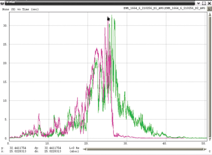
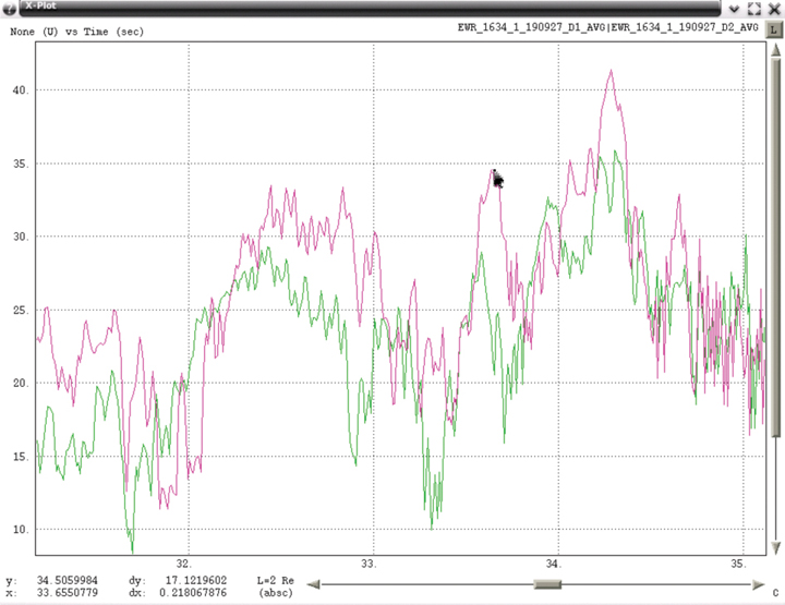
Processed RFI data does display some of these characteristics but with some important differences. PPD power was measured once every millisecond using Snapshot System data and total power within the bandwidth of that PPD was calculated. Total power from both the PCTEL (green) and AEL (pink) antennas were then plotted together with one example for a southbound PPD in Figure 16 and a northbound PPD in Figure 17.
FIGURE 16. RFI Power of southbound PPD (click to enlarge.)FIGURE 17. RFI Power of northbound PPD (click to enlarge.)
Although the envelope of the measured average power tends to have the shape that modeling predicts, there are significant variations over short periods of time. Figure 18 expands a portion of one example and indicates that RFI power varied by more than 17 dB in 0.2 seconds. Examination of spectral data for time intervals of less than one second frequently contains significant changes in observable power. Swept CW from PPDs should exhibit relatively flat RF spectral power, but typical observed spectra include sloping across the band and notches. Possible explanations for these observations include: blockage and diffraction from other vehicles near the one containing the PPD, multipath from other vehicles on the NJT, and the effect of transmitting from within a vehicle. Although some of the snapshot captures exhibit smooth power variation similar to predicted, the vast majority of the hundreds of snapshots exhibit significant variations in power.
FIGURE 18. RFI Power of southbound PPD (expanded).
Examples of Observed PPDs
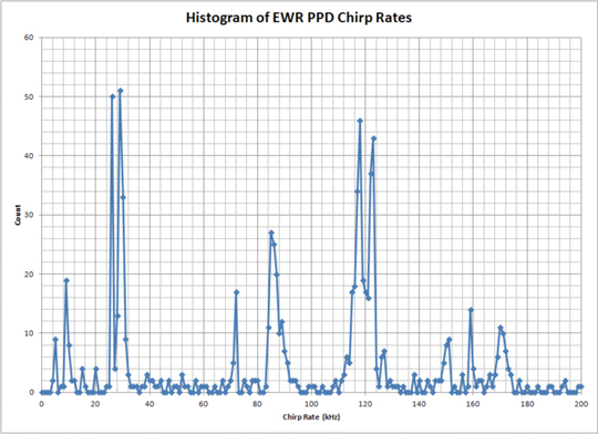
The variety of PPDs observed by the updated EWR monitoring equipment has been surprising. Within its first month of operation, more than 40 PPDs were observed with no less than 19 from unique and different PPD transmitters. Classification of PPD transmitters is based on the combination of RF spectra and the spectrum of the FM demodulated data. Although the observed PPD transmitters use a linearly swept FM sawtooth, most contain deviations from a pure linear sweep. Figure 19 shows examples of FM demodulated time series. Rather than attempting to uniquely describe the attributes of each type of deviation, it is simpler to compute the spectrum of the FM demodulated data. The fundamental frequencies of chirp rates that have been observed have spanned 9 kHz to 170 kHz. Figure 20 shows a histogram of chirp rates observed near EWR and indicates that the most frequent rates have been 9, 26, 29, 72, 85, 118, 123, 159 and 170 kHz.
FIGURE 20. Histogram of EWR PPD chirp rates.
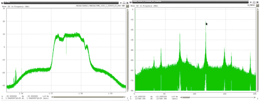
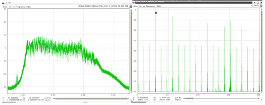
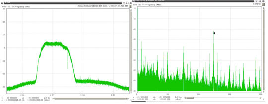
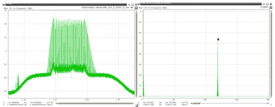
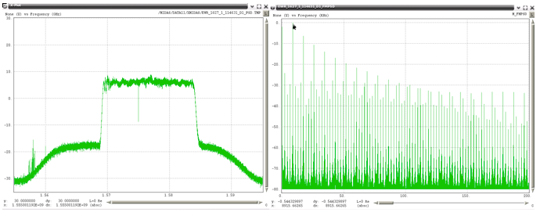
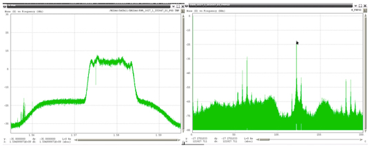
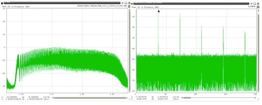
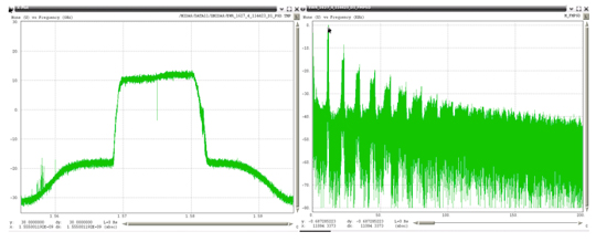
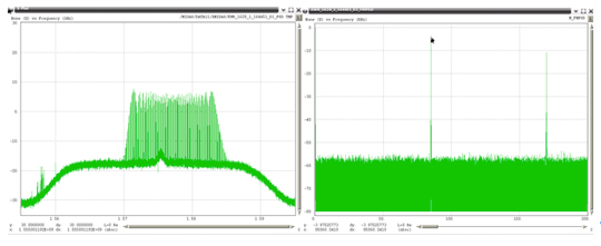
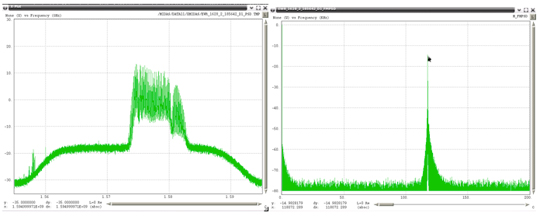
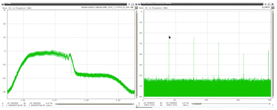
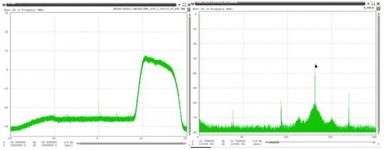
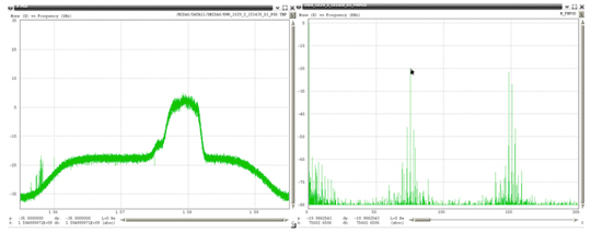
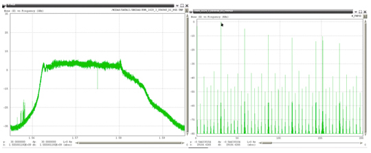
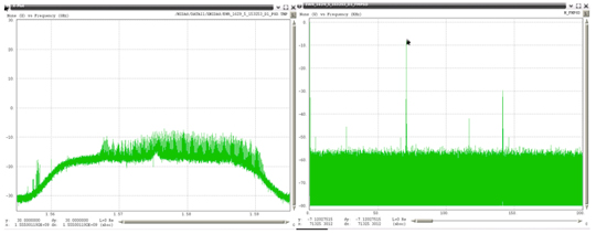
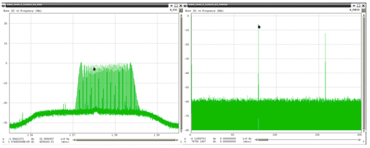
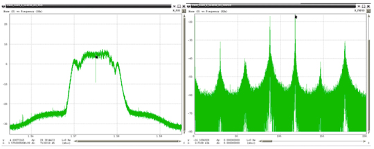
Examples of the 19 unique PPDs (detected within one month) are shown in Figure 22 through Figure 40, with the RF spectrum shown on the left, and the spectrum of the FM demodulated shown on the right. In each of these plots the scaling for the RF spectra is identical, spanning 40 MHz centered on 1575 MHz with a vertical scale using 10 dB per grid. All of the FM demodulated spectra use a horizontal axis that spans 0 to 200 kHz. For references purposes Figure 21 shows the RF spectra when no RFI is present.
Some of these PPDs were transmitting at power levels (observed by the PCTEL antenna) as much as 40 dB above the LNA noise floor. Most spectra were not centered symmetrically about L1 with some completely outside the mainlobe of the GPS C/A code. A few were transmitting outside the programmed 40 MHz bandwidth of the Snapshot System (1555 to 1595 MHz). For those PPDs transmitting outside this band, estimates were made of the upper or lower frequencies using the linear slope of the FM demodulated data, and then extrapolating that slope based on the chirp interval.
Some of the FM demodulated spectra contain a single spectral line that indicates the waveform modulating the RF has a very linear sweep. Most contain additional harmonic lines about the major component and a few appear to have bandwidth about their main spectral component. The current hypothesis is that many of these devices are poorly shielded and that the internal oscillator used to modulate the RF is affected by other nearby signals that are then appearing at the RF output. Some of the possible sources could be circuits that are within the device itself but there is some evidence that a few of these devices are susceptible to energy external to the PPD. A Snapshot System located near Houston International Airport (ZHU) has captured data from PPDs that contain strong components at 58.7 Hz in addition to its linearly swept 97 kHz waveform. Since this frequency is sufficiently different from utility AC power sources (60 ± 0.03 Hz), it has been hypothesized the vehicle carrying that PPD, also has a power inverter. Most power inverters are specified to provide a frequency output of 60 ± 3 Hz. Figure 32 shows a spectral notch that was present at that single frequency throughout the complete capture and suggests that that particular device may have had an impedance matching problem in its transmission path.
FIGURE 21. Spectra with No RFI Observed by PCTEL (click to enlarge).FIGURE 22. 1570 to 1583 MHz, Chirp 117.35 kHz.FIGURE 23. 1556 to 1583 MHz, Chirp 28.43 kHz.FIGURE 24. 1565 to 1578 MHz, Chirp 123.13 kHz.FIGURE 25. 1568 to 1583 MHz, Chirp 111.08 kHz.FIGURE 26. 1578 to 1589 MHz, Chirp 118.07 kHz.FIGURE 27. 1568 to 1584 MHz, Chirp 8.92 kHz.FIGURE 28. 1572 to 1584 MHz, Chirp 121.93 kHz.FIGURE 29. 1557 to 1622 MHz, Chirp 36.14 kHz.FIGURE 30. 1568 to 1582 MHz, Chirp 11.08 kHz.FIGURE 31. 1570 to 1585 MHz, Chirp 85.06 kHz.FIGURE 32. 1572 to 1582 MHz, Chirp 118.07 kHz.FIGURE 33. 1529 to 1577 MHz, Chirp 39.52 kHz.FIGURE 34. 1578 to 1594 MHz, Chirp 131.33 kHz.FIGURE 35. 1575 to 1582 MHz, Chirp 75.66 kHz.FIGURE 36. 1561 to 1586 MHz, Chirp 29.16 kHz.FIGURE 37. 1568 to 1592 MHz, Chirp 71.33 kHz.FIGURE 38. 1560 to 1595 MHz, Chirp 9.88 kHz.FIGURE 39. 1564 to 1582 MHz, Chirp 100.48 kHz.FIGURE 40. 1584 to 1599 MHz, Chirp 128.20 kHz.
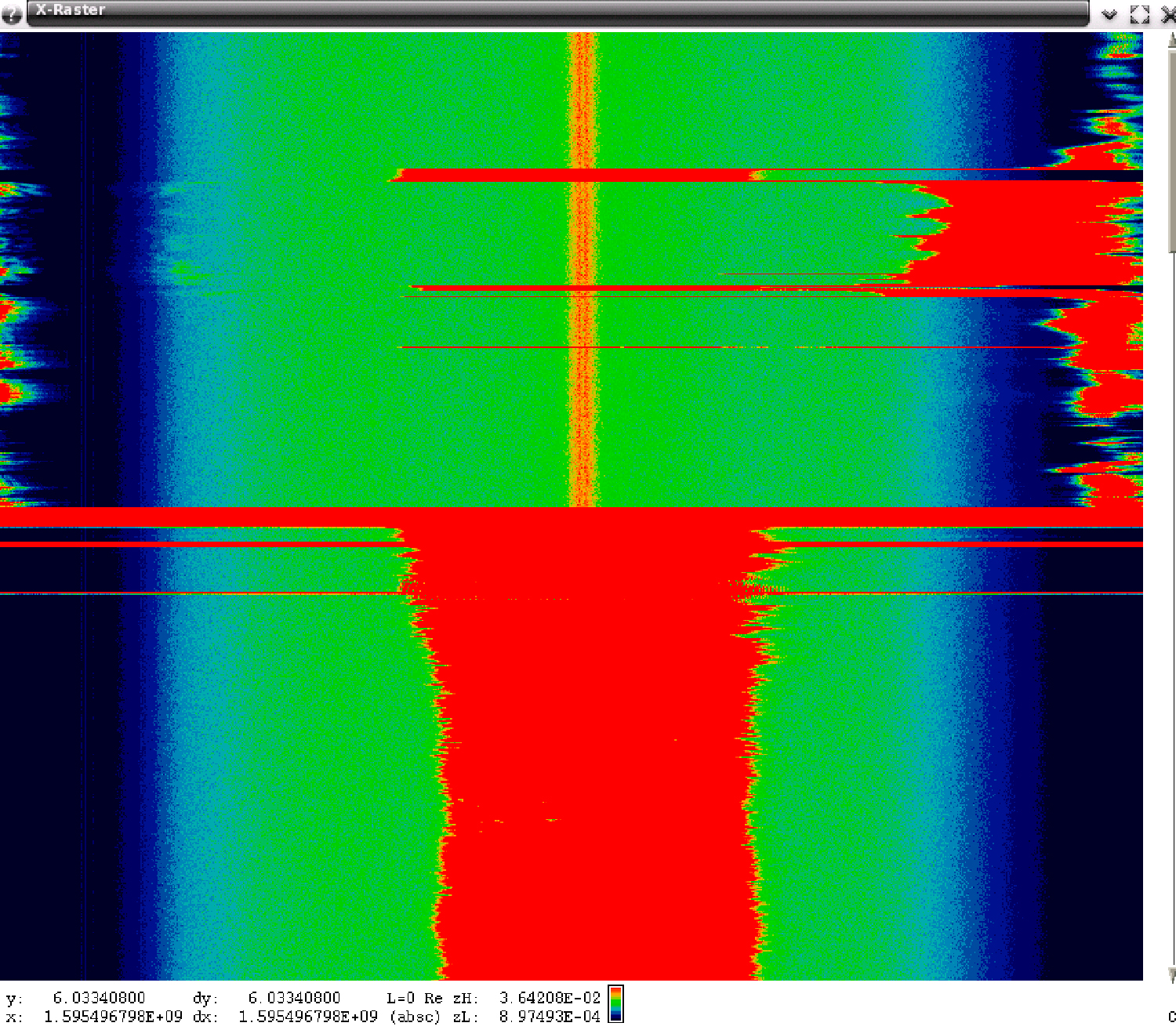
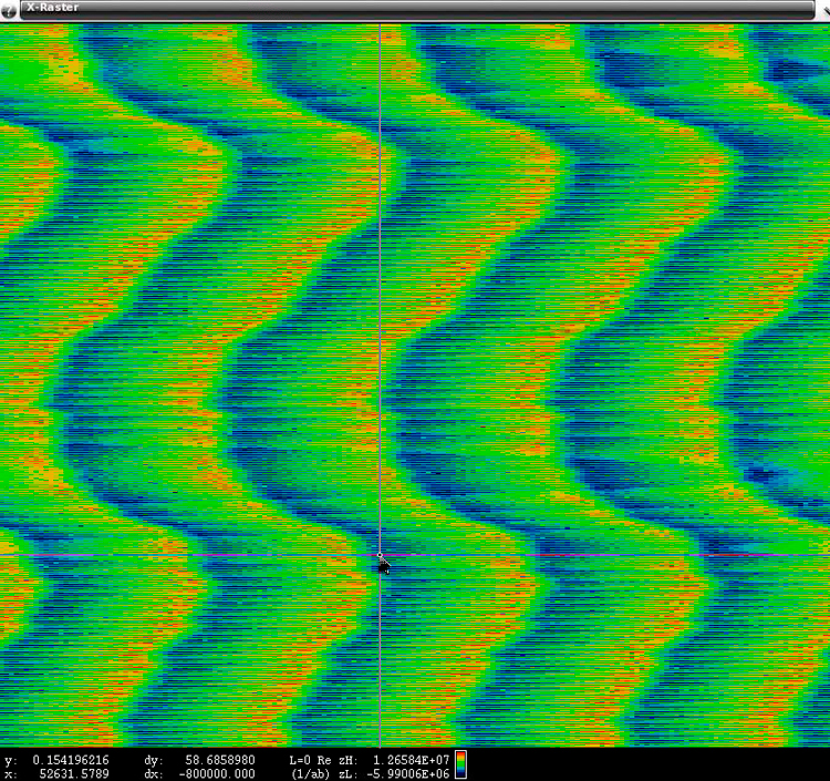
A few snapshots have also provided evidence that some of the PPDs are erratic and probably not functioning as their manufacturer intended. Figure 41 contains a raster of 6 seconds of spectral data that shows a PPD whose output was meant to be between 1560 and 1580 MHz but for short periods of time was transmitting at frequencies above 1580.
FIGURE 41. Spectral Raster, PPD with Unstable Output.
Remarks on Additional PPDs
Since April 2011 the Snapshot System has captured many additional and different PPDs. No effort has been carried out to catalog all of the different types that have been observed but the following describes interesting and notable PPDs.
Figure 42 shows characteristics of a PPD that has had estimated EIRP approaching +20 dBm, to a point just outside the vehicle, and has also been associated with GPS receiver C/N0 degradation of more than -27 dB, strong enough to cause the WAAS receiver, located at the GBAS shelter, to lose lock on all GPS satellites for a short period of time.
FIGURE 42. 1568 to 1582 MHz, Chirp 118 kHz
Figure 43 shows a PPD that is one of the most frequently observed PPDs but that has not been associated with any significant degradation to the GPS receivers. Estimated EIRP for these PPDs has been on the order of no more than +10 dBm. One device with similar characteristics was procured and its measured power at the antenna output port was no more than +14 dBm. Marketing information on the internet for that PPD specified its output power as +25 dBm.
FIGURE 43. 1572 to 1589 MHz, Chirp 85 kHz.
Figure 44 shows a PPD that is transmitting at both L1 and L2. The EWR Snapshot System has been configured to only capture snapshot data at L1 due to the fact that LAAS only uses L1. However, the WAAS receiver used to monitor for RFI is a dual frequency receiver that on occasion has indicated simultaneous RFI at both L1 and L2. Even though the EWR Snapshot System has not captured data at L2, the simultaneous presence of both L1 and L2 RFI, provides strong circumstantial evidence that this RFI source was transmitting on both frequencies. A Snapshot System monitoring the WAAS Reference Station (WRS) at Leesburg Virginia has captured simultaneous L1 and L2 RFI events. Demodulation of that data indicated the two RF outputs had similar modulation but the demodulated data was not coherent. Therefore, that PPD was probably using individual, but similar waveform generators, for each RF output.
FIGURE 44. 1562 to 1583 MHz, Chirp 114 kHz.
Almost all PPDs have been observed individually. However, there have been at least three times in the last two years when two unique PPDs have been observed within 60 seconds of each other. Figure 45 plots normalized degradation in C/N0 while Figure 46 plots snapshot measured power for the same RFI event. Analysis of snapshot data for each of the times that had strong RFI power are shown in Figure 47 and Figure 48 and confirmed that there were in fact two unique PPDs observed approximately 40 seconds apart. Both were traveling south on the NJT and approximately 1200 meters apart.
FIGURE 45. Normalized C/N0 August 19, 2011FIGURE 46. Snapshot Power August 19, 2011.FIGURE 47. C/N0 -19.0 dB, Chirp Rate 78.97 kHz.FIGURE 48. C/No -28.0 dB, Chirp Rate 117.24 kHz.
Most of the observed RFI events last for no more than 50 seconds although a few that lasted much longer have been correlated with slow traffic on the NJT. Figure 49 is from June of 2010, before the updated monitoring equipment was in place, and displays normalized degradation of C/N0. The time duration for which this RFI was observed was more than 3 minutes and was during a time when traffic was ‘slow’ on the NJT.
FIGURE 49. June 9, 2010, PPD, Estimated Velocity 10 m/s.
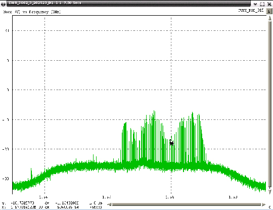
Very wide-bandwidth PPDs have recently been observed more often. The frequency span these devices are transmitting has had to be estimated due to the fact that the Snapshot monitor has 40 MHz of bandwidth, and these PPDs are transmitting beyond this bandwidth. Figure 50 through Figure 52 show examples of these types of PPDs. The left plot in these figures is the RF spectra and the right plot is the FM demodulated waveform. The latter each contain a linear component that is present for only a portion of the chirp interval. Under the assumption that the modulating waveform would be linear for the repetition interval, the slope of the visible linear component was extrapolated to the total chirp time interval. It is not possible to estimate the upper and lower frequency points for the last two examples, since neither of those had a frequency that began or ended within the observable 40 MHz bandwidth of the monitor.
Although the Snapshot System L-band tuners can be programmed for greater bandwidth, the limiting bandwidth is the bandpass filters contained within the LNA modules, which have bandwidths of 40 MHz.
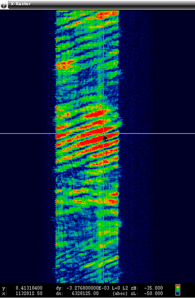
Data captured by a Snapshot System operating near ZHU contains evidence that external energy may have coupled into that PPD and affected the modulation waveform. Figure 53 shows a plot of the RF spectra and an expanded portion of the FM demodulated spectra indicating the presence of a 58.7 Hz component. A raster of the demodulated FM, shown in Figure 54, highlights the 58.7 Hertz component.
FIGURE 53A. ZHU chirp 118 kHz with 58.7 Hz.FIGURE 53B. ZHU chirp 118 kHz with 58.7 Hz.FIGURE 54. ZHU raster of FM showing 58.7 Hz (Click to enlarge).
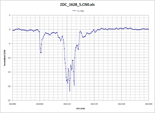
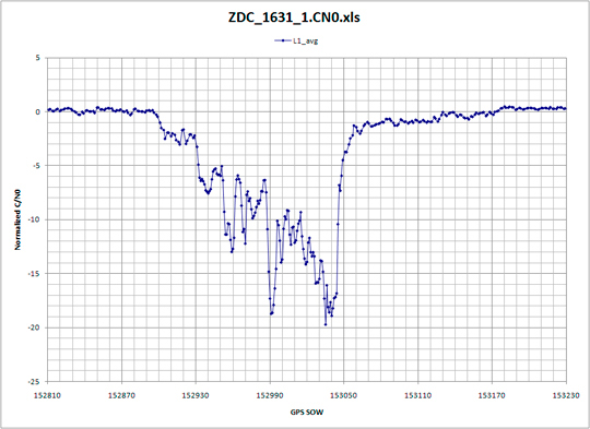
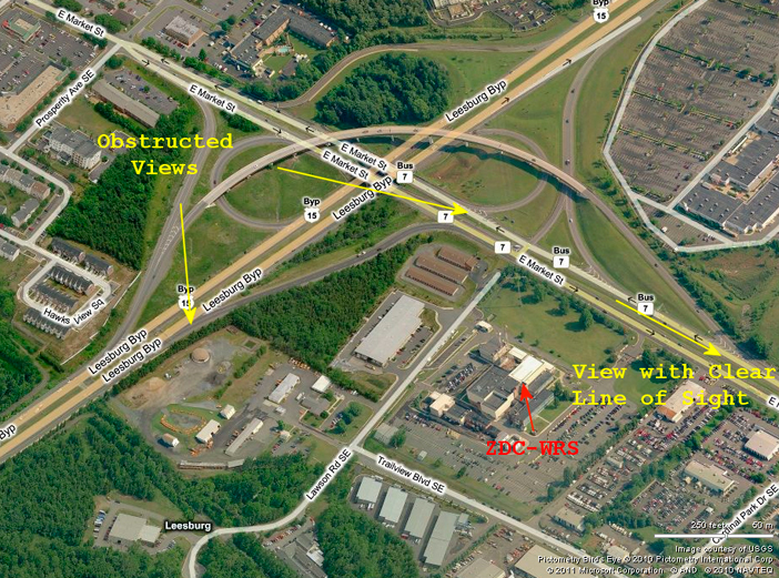
Careful analysis of normalized C/N0 has also provided clues as to the possible travel paths that a PPD might be using. RFI was suspected at the WRS located at Leesburg Virginia (ZDC). A Snapshot System was installed to detect and characterize possible RFI. Analysis of snapshot data did confirm that a few PPDs were traveling past ZDC. One of the PPDs was more disruptive than the others but fortunately was also following a very predictable schedule. It was regularly detected twice a day, first within 10 minutes of 4:30 AM local and next within 30 minutes of 2:30 PM. Normalized C/N0 contained similar patterns for each time of day and are shown in Figure 55 and Figure 56. Examination of the local roadways, shown in Figure 57, suggested the possible roads and direction in which this PPD was traveling. The WAAS antennas on the roof of ZDC have clear line of sight to state highway 7 for vehicles that are east of ZDC. Normalized C/N0 for morning events tended to have a relatively abrupt onset followed by a gradual return to normal while the afternoon events exhibited a gradual increase in degraded C/N0 followed by a quick return to normal. This observation lead to hypothesizing that the PPD was traveling east in the morning and west in the afternoon.
FIGURE 55. ZDC Typical Morning Degradation.FIGURE 56. ZDC Typical Afternoon Degradation.FIGURE 57. Roads near ZDC (click to enlarge.)
FAA Spectrum personnel were informed of this analysis and confirmed that this hypothesis was correct. Using this information they were able to detect the vehicle that was responsible and remove this particular PPD from service.
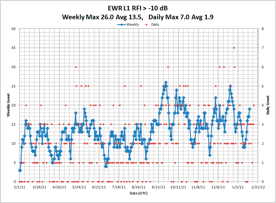
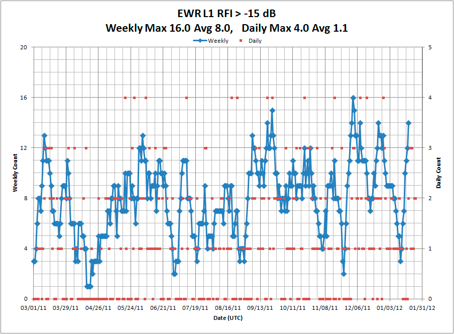
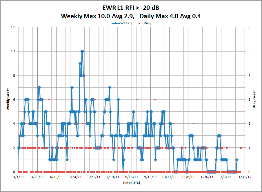
EWR RFI Event Statistics
A large number of RFI events have been detected at EWR since the updated Snapshot System was installed on March 3, 2011. These RFI events have been ranked according to the magnitude of degradation in normalized C/N0, as reported by the GBAS shelter WAAS receiver. The following plots show the total number of RFI events per day (red dots) and for every seven consecutive days (blue line). On average, PPD-induced receiver degradation of at least 10 dB has been observed two times a day. Although a small number of narrowband RFI events produced receiver degradation of as much as 10 dB, the vast majority of RFI events causing 10 dB or more of receiver degradation are due to PPDs.
Figure 58 indicates that since March 2011, more PPD RFI events are being observed. However, Figure 60 indicates that the higher-power PPDs are not being observed as often. One possible explanation is that the previously observed PPDs have stopped working, and the individuals using them have either not acquired replacements or they have acquired different ones with less-damaging RFI.
FIGURE 58. History of RFI > –10 dB (click to enlarge).FIGURE 59. History of RFI > –15 dB (click to enlarge).FIGURE 60. History of RFI > –20 dB.
Many recent PPDs have been transmitting with estimated frequency spans of 65 MHz to 140 MHz. Although the estimated EIRP of many of these very wide bandwidth PPDs has been as much as +10 dBm, their effect on GPS receiver processing has not been as damaging due to the fact that the RFI is within the GPS receiver processing bandwidth for only a portion of the time.
Spectra of Swept FM with Multipath
One of the most commonly observed characteristics in PPD spectral data has been uniformly spaced nulls as shown in Figure 61 and Figure 62. Figure 63 displays a spectral raster that shows how the nulls shift in frequency over time. Initially, there was uncertainty as to the mechanism responsible for these observations. Under the hypothesis that multipath might be responsible, a single ray multipath model was used to predict the spectral characteristics of a PPD that includes a multipath component. This analysis was pursued in the hope that it might provide additional information as to the exact location of PPDs.
The swept CW signals used by PPDs provide a useful source for characterizing multipath between the PPD and monitoring antennas. Equation (1) models observed CW that is the sum of the direct path and a single reflection in which reflected component has a path length difference of d meters.
(1)
Assuming the reflection is from a metal surface, it should experience a phase reversal. Therefore, destructive cancellation between the direct and multipath component will be present for those frequencies that have a path length difference that is an integer multiple of the wavelength. Equation (2) represents this condition.
(2)
Simplification results in the following expression.
(3)
As an example, if spectral nulls are observed at intervals of 10 MHz, then the path length difference is approximately 30 meters. Spectral nulls have been observed at frequency intervals ranging from 2 MHz to as much as 30 MHz. These null spacing’s translate to path length differences of between 150 meters to 10 meters. Multipath with a path length difference of less than 8 meters will exhibit a single null in the 40 MHz bandwidth of the Snapshot System and therefore cannot be estimated accurately using this technique. A path length difference of 8 meters is also what might be expected for two vehicles traveling side by side on interstate highways since interstate highway specifications require lanes to be approximately 4 meters wide.
Once a possible mechanism for the spectral nulls was hypothesized, additional analysis was performed on specific RFI events in which uniformly spaced spectral had been observed. Snapshot and GPS receiver data indicates the direction of travel for a PPD. With direction of travel known, it is possible to approximate the distance that the PPD is from the monitoring equipment. However, for those RFI events that were examined, the calculated path length difference was similar to or greater than the distance between the PPD and monitoring equipment. The most likely location of surfaces that would reflect the PPD transmission was other vehicles on the NJT. Had the surfaces responsible for the reflections been stationary objects nearby, then it might have been possible to hypothesize the most likely location of the PPD by combining receiver proximity and path length differences.
The magnitude of the reflection coefficient can be estimated by comparing the relative power of the spectral maximum and minimum. However the magnitude of the reflection coefficient can only be bounded since it depends on both the reflection coefficient and the relative path length difference. Since the reflected path travels farther, its magnitude will inherently be reduced, in addition to the loss from the reflection, and therefore the observed relative difference will be smaller than shown by equation (4).
(4)
For the examples shown in Figure 61 and Figure 62 the spectral max/min was on the order of 10 dB. By using 10 dB for SpectraMaxMin in equation (4), a reflection coefficient of at least 0.5 is calculated. Reflection coefficients of trucks with shipping containers will probably be much greater than 0.5 and could easily be as high as 0.9.
Direction-Finding Methods
After examining more than a thousand examples of PPDs and their effect on GPS receivers, I have concluded that any type of ground-based direction finding system intended to detect and locate low power moving PPDs over a large area using time-difference-of-arrival (TDOA) or beam forming (angle-of-arrival, AOA) techniques will face significant challenges.
Accuracy of TDOA-based location systems can be decomposed into two components: measurement accuracy, and the geometry of the equipment used to make these measurements. In 1982, Paul Chestnut calculated the relationship between accuracy and these two components, showing that geometry is a multiplicative factor. Direction-finding conceptual design typically strives to position the measurement equipment such that it surrounds the area to be monitored, if possible. For those situations where it is not possible to encircle the area, the measurement equipment will typically have a long baseline between its sensors and with a perpendicular orientation with respect to the monitored area. This strategy reduces errors due to geometry.
Measurement error depends on the observable power of the signal to be located. This component will most likely limit the ability to accurately locate low-power moving PPDs. Measurement data from GPS receivers demonstrate the ability to reliably detect the presence of these PPDs, but only when they have been within hundreds of meters. Most PPDs have been observed for 30 to at most 60 seconds. For PPDs traveling along the NJT at a velocity of 30 m/s, this time span implies that they were not detected until they were within 900 meters. Reliable detection was not demonstrated unless they were within 500 meters. This is a direct consequence of the fact that all GPS antenna are designed for hemispherical coverage for satellites above the horizon. The PPDs are at the horizon or lower relative to most GPS antenna patterns. If GPS antennas were used as part of a TDOA-based system, they would need to be positioned no further apart than approximately 600 meters. Using GPS antennas to detect and locate PPDs is inherently limited to proximity detection.
The ability to locate low-power PPDs within a larger area requires a system to be able to detect a PPD by all of its sensors simultaneously from distances much greater than 600 meters. In principal, higher-gain antennas orienting their main beam along the NJT would increase the distance over which PPDs could be detected. Even when high-gain directional antennas have been positioned along the NJT, the observed power has not followed predictions based strictly on FSL. One reason for this is that clear line-of-sight could not be achieved between the high gain antenna and the PPD. Vehicular effects might also be responsible for these observations. What is known is that the power observed by ground-based antennas has shown significant fluctuation, much greater than could be explained by FSL propagation. Ground-based direction finding systems for low-power moving PPDs must be able to simultaneously detect RFI by multiple sensors, in an environment that may at times shield the PPD from its sensors, and that also has fluctuating observable power.
The ability to observe, detect, and locate low-power moving PPDs over a large area would require a system to have its monitoring antenna located high above the NJT, and oriented to look down on the NJT and the surrounding area. Although such a system must still contend with shielding from the vehicle itself, it would be the only approach that could potentially observe these PPDs over a large area, simultaneously by all of its measurement sensors. Implementing such a concept may be expensive.
A less expensive approach might rely on proximity detection, with many sensors on the ground, each monitoring their own small area, and only report PPDs that travel close to each of them. One such approach, referred to as crowd sourcing, uses cell phones to aid in detecting and locating PPDs. Crowd sourcing is a form of proximity detection.
Summary
The first evidence of low-power moving PPDs along the NJT used two GPS receivers separated by considerable distance and then correlated their responses. This approach is only useful for detection of PPDs traveling in close proximity to the GPS receivers. Analysis of GPS receiver normalized C/N0 also provided a basis for determining if RFI might be from a moving emitter. The shape of normalized C/N0 versus time not only provides clues that the RFI source is in motion, but may even be correlated with their possible travel paths, when blockage exists between the GPS antenna and local roadways.
Autonomous operation is a necessity for detecting low-power moving PPDs, since they may be observable only a few times a day and for less than 60 seconds.
Capturing real-time samples of these intermittent RFI events determined the existence of many different types of PPDs. Almost all use some form of swept FM modulation. Analysis of their spectra and modulation indicates that many devices are probably not operating as their manufacturer intended. Modulation waveforms of PPDs have included triangle, highly linear sawtooth, sawtooth with synchronous perturbations on top of the fundamental sawtooth, and sawtooth with analog modulation. The leading hypothesis for this observation is that the devices are not shielded very well and that the internal modulator is susceptible to coupling from either other circuits within the PPD itself or from external electronic devices operating in the vicinity of the PPD.
Acknowledgments
The author thanks the FAA for support in this investigation, Rich Holley of ICE-Online for help in utilizing capabilities of the ICEPOD6-M5, and Julian Babel of the FAA Technical Center for regularly swapping external hard drives attached to the Snapshot System.
Joe Grabowski is a systems engineer at Zeta Associates where he works on a variety of GPS projects in support of the FAA, as well as communications systems and digital signal processing applications. He received an M.S.EE from Purdue University. Since 2010 he has been involved in the investigation of personal privacy device impacts on FAA SBAS and GBAS sites.
DigitalGlobe announced two licensing agreements with Microsoft.
According to the announcement, the first agreement more than doubles the volume of high-resolution imagery DigitalGlobe delivers to Microsoft for use in its Bing Maps service. The imagery, delivered on a quarterly basis, will provide refreshed content covering millions of square kilometers of the earth’s surface, including up-to-date imagery for the world’s highest-density urban areas.
“We’ve chosen to expand the use of DigitalGlobe satellite imagery to provide broader global coverage in Bing Maps,” said Steve Stanzel, general manager at Microsoft. “With this increase and our continued work with DigitalGlobe for the collection of high-definition aerial imagery, we are improving our maps worldwide to offer a more comprehensive, consistent and functional mapping experience.”
DigitalGlobe reports the second agreement enabled Microsoft Studios to extensively feature DigitalGlobe imagery in the recently launched Forza Motorsport 4 racing game for the Xbox 360. The Forza Motorsport series is one of the world’s most realistic and successful racing franchises. The latest installment, Forza Motorsport 4, features the first-ever combination of DigitalGlobe satellite and Microsoft aerial imagery into a seamless gaming experience, resulting in unprecedented, true-to-life detail.
Forza 4 game designers selected many high altitude and low altitude images for each track region featured in the game and combined them into a seamless animation sequence, using advanced memory management techniques. The result gives players the experience of travelling across the globe in Forza Motorsport 4’s World Tour mode.
Both agreements took effect in the fourth quarter of 2011.
“We are proud to know that DigitalGlobe content plays a valuable role in helping Microsoft achieve its business objectives and deliver a superior, photo-realistic experience for its end-users,” said Rafay Kahn, senior vice president at DigitalGlobe. “We look forward to a successful, ongoing relationship with Microsoft in order to support the millions who use their products and services every day for insight, understanding and entertainment.”
Blue Marble Geographics announced the release of Global Mapper Software Developer Toolkit version 13.1. This update features many new drawing and analysis tools along with enhanced geospatial PDF and LAS 1.4 support.
According to the announcement, Global Mapper SDK 13.1 syncs up the software developer toolkit with Global Mapper desktop software releases. This will enable a more consistent release cycle ensuring the software developers are able to work with the latest and greatest feature/functions introduced to the desktop version of the software. The 13.1 release introduces many new drawing tools such as drawing map layout items, including elevation legend, distance scale, map feature legend, and north arrow. The update also introduces powerful new analysis tools like the function for creating density/heat grids from loaded point features, the function for creating roughness length grids from a land cover layer and the method for easily calculating a watershed with stream paths and drainage basins from loaded terrain layers. The ability to add custom online data sources is introduced along with improved Geospatial PDF support, new LandXML, LASzip and LAS 1.4, I.H.S. Well Data point files, GeoJSON, and Digital Bathe Bathymetric Database Variable Resolution (DBDB-V) files and much more.
“Blue Marble has been directly supporting hundreds of geospatial software developers implement cutting edge technology for years,” stated Blue Marble President Patrick Cunningham. “The Global Mapper SDK is a great tool to add to a suite of libraries and we are excited to work directly with our developer community with this new display and translation api. Syncing up the SDK kits with the desktop releases will help us provide the latest features and functionality to our existing users as well as new customers for future releases.”
Blue Marble’s geospatial data manipulation, visualization, and conversion solutions are used worldwide by thousands of GIS analysts at software, oil and gas, mining, civil engineering, surveying, and technology companies, as well as governmental and university organizations.
Blom announced that BlomURBEX imagery was integrated into Finland’s most popular web mapping service, Fonecta’s Enrio.fi. Integration was done using BlomURBEX’s API (Application Programming Interface) tools.
According to the announcement, the oblique imagery served from BlomURBEX provides users with a rich, interactive and highly informative view of the area of interest. For example, before setting off to a destination, users can inspect Eniro.fi’s routing services. The oblique imagery provides a broader visual understanding of the area, and helps users to easily locate themselves within their surroundings.
“We are developing all of our services to help people and companies in everyday tasks, and customer feedback is very important for us. For some years Blom has provided us with oblique images and these have always generated a lot of interest with an established user base,” states Toni Wistbacka, the Product Manager of Eniro.fi –service.
Blom reported that in addition to oblique and ortho imagery, several types of map layers, and routing service functionality, Fonecta’s improved Eniro.fi service also provides tools for searching contact information of companies and individuals in Finland.
GeoExperts announced that Hamilton County, Ill., is using GeoSpatial Experts’ GeoJot field data collection app on an iPad to correlate street addresses with parcel coordinates. Initiated for tax assessment and E911 purposes, this photo project is creating the rural county’s first digital map database that matches property addresses to their correct geographic locations.
“Most houses have been assigned streets addresses, but they’ve never been correlated to our county parcel database,” said Mark Becker, Hamilton County Supervisor of Assessments. “People still have to give their address verbally when they call 911 for assistance.”
Hamilton County is rapidly updating its address and property database to meet E911 standards using the iPad and GeoSpatial Experts’ GeoJot application, according to Becker. GeoJot is an easy-to-use app that converts an iPad or iPhone into a field data collection device. Available from the Apple App Store, GeoJot is a companion application created for exclusive use with the PC-based GPS-Photo Link photo-mapping software. GPS-Photo Link is able to map photographs and accompanying attribute information captured with a GPS camera, smartphone with GPS, or any digital camera used in conjunction with any GPS unit. Digital map output includes Esri shapefiles and geodatabases as well as Google Earth files.
In Hamilton County, college interns walk from house to house taking photos of each one with the iPad 2. They then key in the house number, street name and street direction to keep the Assessor’s tax database up to date. These attributes – along with the GPS coordinates – are permanently linked to the correct property photo by GeoJot. Back at the Assessor’s Office, the GeoJot files are uploaded to the GPS-Photo Link photo-mapping software running on a PC.
“Mapping addresses will save money for Hamilton County by making its assessment activities more efficient,” said GeoSpatial Experts’ President Rick Bobbitt. “More importantly, an accurate address map is a necessity for timely E911 response to emergency calls.”
In 2011, GeoSpatial Experts introduced GeoJot to leverage and maximize the built-in geotagging capabilities of the camera-equipped iPad and iPhone. These mobile devices use internal GPS chips to stamp each photo with location coordinates where the photo was taken. GeoJot maximizes the geotagging accuracy of the internal GPS chips by up to four times – putting it well within the accuracy specifications of many business-related photo-mapping applications.
Telogis, Inc. announces the acquisition of the assets of Maptuit, a leading provider of connected navigation for commercial fleets. This acquisition — the company’s fifth in three years — expands Telogis’ services as the market increases adoption of location-based Software-as-a-Service (SaaS) solutions. Maptuit’s commercial navigation technologies further enhance the Telogis enterprise platform of SaaS solutions, which includes fleet management, navigation, multi-vehicle route optimization and planning, work order management and mobile integration.
“This acquisition adds a new dimension to our platform,” said Newth Morris, president, Telogis Route and Telogis Mobile. “With these advances, Telogis further differentiates itself in the market by providing the most comprehensive suite of location intelligence solutions on a single platform.”
According to the announcement, the enhancements to the Telogis platform resulting from this acquisition include an advanced location-based service (LBS) engine that receives feedback from the field on road conditions and physical restrictions that may not be captured by commercial and open source map data. These capabilities are critical not only to the commercial navigation markets where Maptuit has been successful, but also to industries such as mining, and oil and gas, which operate in remote regions where map data coverage is limited.
Maptuit’s technologies also allow companies to specify “known-good” routes and yard-approaches. These capabilities help companies improve the safety of route operations and are increasingly important in international markets where bonded routes exist.
Telogis reports it will integrate Maptuit’s technologies directly into its enterprise platform, thereby expanding the Telogis customer base by more than 100,000 subscribers.
“The commercial navigation technologies that Maptuit has revolutionized will enhance all of the applications on our platform — route planning, navigation, execution analytics — and position our company to best handle the growing location intelligence needs of companies worldwide,” said Morris. “This acquisition complements the Telogis platform with a unique set of high-value capabilities that allow companies to dramatically transform their operations, improve safety and lower operating costs.”
Esri announced that the Strauss Center’s Climate Change and African Political Stability (CCAPS) program has implemented Esri technology to view how climate change impacts vulnerable populations in Africa. CCAPS created the dynamic mapping tool in partnership with AidData for use by researchers, policy makers, journalists, and citizens. Users can visualize any combination of CCAPS data on climate change, conflict, and aid on a map to discover how different forces overlap or intersect.
“This mapping tool allows policy makers to analyze data from multiple sources at once, providing integrated analysis of the drivers and responses related to security risks stemming from climate change,” said Francis J. Gavin, director of the Strauss Center.
According to the announcement, the tool is already being used in the country of Malawi for a solution that tracks and reports on the country’s external funding. Aid information is mapped along with data on climate change vulnerability and incidents of conflict. This sheds light on whether aid is effectively targeting regions where climate change or conflict poses the most significant risk to the sustainable development and political stability of the country.
“Climate change poses an enormous threat to the livelihoods of millions of Africans,” said Jean-Louis Sarbib, CEO of Development Gateway. “The level of risk, however, is not evenly spread and certainly doesn’t respect national boundaries. To ask critical questions about how development assistance can reduce vulnerability, you need hyperlocal data on climate and also on aid-funded interventions. This is what the new CCAPS mapping tool shows in a digestible, interactive way.”
Esri reported that by integrating CCAPS research on climate change, along with existing datasets such as topographic maps, imagery, and thematic information on conflicts, the CCAPS mapping tool aims to provide the most comprehensive view possible of climate change and security in Africa.
“The great work of these organizations is a real game changer for the development community,” said Jack Dangermond, president of Esri. “Being able to create a tool that allows people to communicate with others all over the world using maps is powerful. I am impressed with the work being done and excited to see what they will think of next.”
Today, Hemisphere GPS announces the Eclipse P300 and Eclipse P301 OEM modules — its next-generation high‑performance compact modules for RTK GNSS applications. Based on new Hemisphere GPS multi-function application firmware and Eclipse GNSS multi‑constellation technology, P300 and P301 provide the ability for tracking commercially available GNSS signals for precise positioning.
P300 is a drop-in board replacement for Hemisphere GPS’ successful Crescent L1 board as well as the first‑generation miniEclipse P200 GPS-only OEM board. P301 is the company’s 20‑pin OEM module configured as a drop-in replacement for a different industry standard interface. Eclipse P300 and P301 improve GNSS positioning performance, particularly with RTK applications, through Hemisphere GPS’ patent-pending SureTrack technology. Benefits include extended and more robust RTK solutions as the rover RTK receiver will process all available signals even if they are not common with the base receiver. RTK solutions are therefore better maintained in challenging environments, with baselines of up to 50 km, and reacquisition times are improved resulting in more robust overall performance, the company said.
P300 and P301 are designed for OEM system integrators who demand the highest level of multi-frequency positioning, accuracy, fast initialization time, and GNSS RTK solutions. Hemisphere GPS’ miniEclipse series includes a single frequency L1 GPS + L1 GLONASS model named P202. Both series are designed for developing integrated high-precision and control applications for geomatics, survey, machine control, and unmanned vehicle solutions.
“P300, P301, and P202 all improve upon our already successful miniEclipse OEM modules adding GNSS support to our most compact modules for excellent accuracy and affordability,” said Phil Gabriel, vice president and general manager, Precision Products, for Hemisphere GPS. “System integrators have a wider range of Hemisphere GPS solutions from which to choose to develop world‑class high‑precision products.”
Measuring 71 mm long and 41 mm wide, miniEclipse allows for easy integration, especially for integrators who are accustomed to Hemisphere GPS’ Crescent and miniEclipse OEM module performance and footprint.
All miniEclipse modules are available through the Hemisphere GPS Precision Products global dealer network.
GPS as a national asset will be highlighted at the 11th GPS Partnership Council, set for May 1 and 2 at the Space and Missile Systems Center at the Los Angeles Air Force Base, in El Segundo, California. The theme of the council is “Our National Asset At Work.” Registration is now open; attendance is limited to 250.
According to the council, “The GPS Partnership Council serves as a means to communicate with GPS stakeholders on present-day activities, future plans, and measures that are in place to ensure GPS remains the world leader for providing space-based positioning, navigation, and timing services to the warfighter and civilian users. Our commitment to mission assurance ensures users around the globe will continue to benefit from improved GPS performance, while we continue acquiring, operating and sustaining GPS as the ‘gold standard’ for positioning, navigation and timing for the warfighter, the nation, and the world.”
Key council members include:
Brig Gen Martin Whelan, director of Requirements, HQ AFSPC/A5
Col Bernie Gruber, director of the Global Positioning Systems Directorate
Anthony Russo, director for National Coordination Office for Space-Based PNT.
The meeting is sponsored by the Los Angeles Chapter of the Armed Forces Communication and Electronics Association and GPS Directorate.
Day 1, Tuesday, covers two topics, “The Enterprise” — a GPS system capability review, and a discussion of “Modernized GPS User Equipment (MGUE),” with an Army future perspective and an MGUE industry panel.
Day 2, Wednesday, covers “GPS at Work for the Nation” in the morning, including GPS’ role for the Department of Homeland Security, the Federal Aviation Administration, NASA, and other agencies. The afternoon of Day 2 looks at “The Warfighter,” with speakers from 2SOPS followed by a panel discussion.
Both days feature opportunities for networking. The final day, Thursday, features the GPS Scramble Golf Tournament.
Attendees can also browse the displays and exhibits during the conference.
Karlsruhe, Germany — Geoinformation holds enormous potential: “Geoinformation plays an important role in all key sociopolitical issues,” said Karl-Friedrich Thöne at the Intergeo Round Table in Karlsruhe. All participants were in agreement with the President of the German Society for Geodesy, Geoinformation and Land Management (DVW), the organization responsible for hosting Intergeo October 9-11, 2012, in Hanover.
However, the experts — including representatives from the worlds of politics and industry — backed different approaches for the leading international industry forum with conference and trade fair. Georg Thiel from the Federal Ministry of the Interior (BMI) called for a “national geoinformation strategy,” while Ernest McCutcheon, managing director of Karlsruhe-based DDS Digital Data Services GmbH, said that “too great an emphasis” was placed on data protection, favouring instead an approach highlighting the benefits of employing geoinformation.
During the discussion held under the banner “Smart Geoinformation — Intelligent Geoinformation for the Future,” Thomas Haupt, responsible for sustainability in his position as the director of PTV Planung Transport Verkehr AG in Karlsruhe, gave an example demonstrating that easier access to data improves the “robustness of systems.” He said that anonymous mobile data could be used instead of models for planning traffic flows, which would also help find a way out of the “data jungle” and into a “healthy mixed forest.” However, DVW President Thöne warned against focusing exclusively on the benefits of geoinformation. The debate on Google Street View, he said, showed that potential risks also had to be included in any discussion. He proposed that “Intergeo should also serve as a platform for adopting an offensive strategy for data protection and data security.”
The first national Inspire Conference will held at the 18th Intergeo in Hanover this year. Inspire is an EU directive for creating a common geodata infrastructure. Under this directive, high-quality geodata from the public bodies of member states should be made available under uniform conditions to support the formulation, implementation and evaluation of European and national areas of policy. “It is our job to put data protection in Europe on a new footing,” Georg Thiel said. The Inspire Conference and Intergeo, he added, are ideal platforms for launching discussions with a view to developing a national geoinformation strategy.
But how does Inspire affect smartphone owners? “Inspire will generate added value,” said Thiel, referring to the simple example of intelligent lawn-mowing robots. “These lawnmowers can use Inspire, for example, to incorporate weather data into their planning and wait for a storm to pass before automatically starting to mow the lawn.” Public administration bodies will make decisions based almost 100 percent on geoinformation, Thiel said.
Hartmut Rosengarten, from Hexagon Geosystems and spokesman for the Intergeo Exhibitor Advisory Board, acknowledged the event as both an international communication platform for the industry and a bridge between professionals and end consumers. “At Intergeo, we have to offer solutions so they can be understood and utilised by everyone,” he said.