With this being my last column in 2010, I’m going to look back at the five significant GPS/GNSS events in 2010 that affected the surveying, mapping, engineering, construction, and natural resource users. Each of these had, or could’ve had, a significant effect on your GPS activities.
These are listed in order of importance with #1 being the most important.
1. GPS 24+3 constellation. The most important GPS/GNSS event in 2010 occurred back in January, when the Air Force announced it was implementing a new GPS 24+3 configuration. You can read about it in in more detail here, but the idea behind it was to eliminate GPS “brownouts.” These are periods in which there are fewer GPS satellites in view, and when combined with obstructions such as rugged terrain or trees or buildings, make GPS difficult to use.
It’s especially an issue with real-time, high precision users (RTK) because RTK technology is satellite-hungry. It needs six or more satellites to provide a robust position solution.
If you recall, in the new 24+3 configuration, there were three satellites moving significantly from their original slots (SVNs 24, 26 and 30). SVN 26 is already at its destination. SVN 26 is scheduled to reach it destination in January 2011. SVN 30 should have arrived at its destination in the past few days.
In addition, three other satellites (SVNs 46, 55, and 56) are being shifted slightly. SVN 55 should arrive at its destination this month. SVNs 46 and 56 are scheduled to begin transitioning in January 2011 and should be complete in May/June 2011.
By now, you should be seeing some improvements in GPS satellite visibility as the 24+3 configuration is almost complete. From the scenarios I plotted in this article, you can see that although you’ll see fewer peaks (high number of GPS satellites in view), you’ll also see fewer valleys (low number of GPS satellites in view). This should increase productivity for RTK users and users in environments where satellites signals are obstructed (such as under tree canopy).
2. Launch of the first GPS Block IIF satellite. Although it doesn’t really help users at this point other than being another satellite to enter service, the Block IIF satellite launched in May is the first to broadcast the third civil signal, L5. The L5 civil signals marks the beginning of a new era in high-precision GPS positioning. The Block IIF launch was the catalyst for the article I wrote I entitled “What’s Going to Happen When High-Accuracy GPS is Cheap?”
It’s just a teaser though, the launch of the next Block IIF isn’t until next summer at the earliest. Then, the next one is ???. They are being launched at a snail’s pace. Remember though, it costs upwards of $200 million to launch a satellite and since there’s already 30+ operational GPS satellites in orbit, it’s hard for the U.S. Congress and the U.S. Air Force to justify speeding up the launch schedule. During the last Air Force briefing I attended, the target was to have 24 satellites broadcasting L5 by 2019.
Block IIF GPS satellite (Courtesy: The Boeing Co.)
3. Continued development of GLONASS. Despite the recent launch failure (three GLONASS satellites crashed into the Pacific Ocean), the Russian Federation was still able to launch six new GLONASS satellites into orbit in 2010, and with another launch scheduled for later this month of the new GLONASS-K1 satellite, that will test the new CDMA capability for better compatibility with GPS.
As it stands, there are 20 operational GLONASS satellites in orbit, with four more offline for maintenance and two reserved as spares. That’s 26 total. Furthermore, after the Dec. 5 launch failure, Russian Federal Space Agency Director Anatoly Perminov vowed to return the GLONASS constellation to 24 operational satellites by March 2011, something that hasn’t been accomplished since the mid-1990s (albeit briefly).
A consistent and healthy number of GLONASS satellites in orbit has given receiver manufacturers more confidence to develop GPS/GLONASS receivers. Just this year, we’ve seen new receivers from several manufacturers that have taken GPS/GLONASS a step further in integrating them into handheld receivers as well as OEM board products.
For users, the benefits are clear, with the new 24+3 GPS configuration and a healthy number of GLONASS satellites in orbit, GPS/GLONASS users are seeing the most satellites in view ever in the history of GPS/GLONASS. Signals from more satellites typically results in more robust positioning and improved productivity due to decreased down-time.
Rocket launch containing three GLONASS satellites
4. Solar activity affect on GPS. Solar activity was eerily quiet in 2010. The big news is that there was no news. There were some minor solar events in 2010, but despite what you may have read, none of them were strong enough or the type that would affect GPS operations.
So, if your GPS receiver didn’t work at times this year, it wasn’t due to solar activity.
With the peak of the current Solar Cycle (SC 24) estimated to occur in May 2013, solar activity should be ramping up in 2011. In August, I conducted a webinar that discussed, among other things, the subject of solar activity on GPS. You can read a summary of it here and even download the webinar presentation.
You can be sure I’m closely monitoring solar activity for any events that look like they will have an effect on your GPS operations. I’m still working on my notification system and will keep you updated on that. Otherwise, the GPS World website is a good source for news in this area.
Finally, I’ll be attending the Space Weather workshop in April 2011. Most, if not all, of the really smart space weather people from around the world gather and confer on space weather. I’ll be writing about what I hear and learn from these folks. But, the sun is a mysterious creature. I like to get definitive answers to my questions, but even some of the brightest scientists I know will answer with “I really don’t know” when I ask them about a certain behavior of the sun. Mother Nature is humbling at times.
Solar Cycle 24 Prediction (Courtesy: NOAA Space Weather Prediction Center)
5. The GEO failures of GAGAN and WAAS. Both the Indian Space Research Organisation (ISRO) and the U.S. Federal Aviation Administration (FAA) were delivered a hard lesson in SBAS GEO satellite management. The SBAS GEO satellites are the ones that broadcast the integrity and correction information to users. They are the critical communications link that connects the SBAS ground infrastructure to the end users. Without them, SBAS doesn’t work.
In April, the ISRO rocket launch of their GAGAN GEO satellite failed, sending the critical GAGAN GEO satellite splashing into the Bay of Bengal. GAGAN is still in testing phase, so no users were affected, but it set back the GAGAN program. However, it didn’t delay GAGAN as much as I thought it might. Another GAGAN GEO is set to launch later this month (as of December 29, the launch date has now been pushed out to Q1 2011) with a second due to launch in the first part of 2012. The ISRO completed its Preliminary System Acceptance of GAGAN just a few days ago. The aviation-certified system is expected to be operational by June 2013. As with other SBAS, test signals usable by non-aviation users will likely be available during the testing phase, as early as 2011.
Also in April 2010, it was reported that the contractor operating one of the FAA WAAS GEO satellites lost communication with the satellite (PRN 135). It was reportedly an unprecedented event. Initially, it was thought that PRN 135 would drift out of usable orbit within a few weeks, leaving North America with only a single WAAS GEO until a new one was brought into service (PRN 133 was already under testing). Things weren’t quite as bad as they seemed as PRN 135 ended up staying in a usable orbit up until PRN 133 testing was concluded.
However, the defunct PRN 135 was at 133° west longitude and PRN 133 is at 98° west longitude. With the remaining GEO (PRN 138) at 107° west longitude, users in northwest Alaska do not have WAAS service. Since none of the GEO satellites are actually owned by the FAA, they have little say in the location of the GEO satellite. The FAA says they are working on putting two more GEOs into service, but that takes time, and it’s not measured in months, but rather years.
I think the hard lesson is not to skimp on SBAS GEO satellites. Perhaps this event will make it easier for the FAA to sell the concept to Congress (for funding).
If you’re an SBAS user, don’t let this bring you down. SBAS is here to stay, and likely you were not affected by any of the above. These past few days, I’ve been looking at SBAS data (and DGPS data) collected over a 24-hour period. The accuracy and stability is pretty impressive.
That leads me into my last subject which is a webinar I’m conducting on January 26, 2011.
If you are using or plan on using GPS for mapping or surveying, you should seriously consider attending this webinar.
Learn the real story behind each of these technologies without a marketing or salesperson’s bias.
Tens of thousands of users around the world utilize GPS/GNSS receivers for mapping, surveying and navigating. Since autonomous GPS/GNSS typically does not provide the needed accuracy, users must rely on a source of GPS/GNSS corrections. There are three sources of GPS/GNSS corrections available to users who desire reliable GPS/GNSS accuracy in the sub-meter to three meter range: SBAS, DGPS and post-processing. Dr. Michael Whitehead, VP of Technology at Hemisphere GPS, will join me in presenting a background on the three technologies as well as the strengths and weaknesses of each.
I’ve known Mike for a number of years. He was an early innovator in the development of SBAS technology at Satloc as well as SBAS and DGPS receiver technology at Hemisphere GPS. He is one of the leading GNSS engineers in the world. I’m particularly excited about this event and promise a lively discussion that’s full of useful information, data, and concepts that anyone using or considering using GPS/GNSS for mapping, surveying, or navigating will find useful.
Have a safe and happy holiday and a Happy New Year. See you next year.
In my last column, I presented the poll results from my November 16 webinar “A Buyer’s Guide to GPS/GIS Mapping Equipment.” I’ve conducted many webinars over the years, and the audiences have been comprised of hundreds (if not thousands) of participants who have the ability to ask questions and also participate on various polls I conduct during the webinars. This column continues the look back at previous polls conducted during the various webinars in 2010 to give you an understanding of what your colleagues are thinking.
August 31, 2010 Webinar: “Solar Activity, SBAS, and 24+3 GPS Constellation Updates”
Poll #1 (Aug. 31, 2010 webinar): How concerned are you about solar activity affecting your GNSS operations?
Gakstatter comment: These numbers don’t surprise me. Personally, I probably fall in the “Somewhat” category, but my GPS/GNSS field work is pretty flexible so I can easily adjust without much inconvenience. However, if I had several crews using GPS/GNSS on a daily or near-daily basis or I had equipment relying on GPS/GNSS, I think I’d be in the “Very” category because the $$ impact would be much higher.
Poll #2 (Aug. 31, 2010 webinar): If it was available, would you be interested in receiving alerts/warnings of solar activity that may affect GNSS operations?
Gakstatter comment: I’m not surprised at these results either. When I initially considered this poll, I was thinking about asking which type of platform you would prefer to receive alerts/warnings with the choices being Droid app, iPhone app, Blackberry app, text message, e-mail, etc. If you have a preference on that, fire off a quick e-mail to me. Secondly, a few of you pointed out that NASA has an app for this, but keep in mind that the system I’m considering is focused specifically on high-performance/precision GPS/GNSS users, which would eliminate a lot of the baggage of the alert/warning systems available today.
Poll #3 (Aug. 31, 2010 webinar): Do any of your GPS receivers use SBAS (WAAS/EGNOS/MSAS) as a primary source of corrections?
Gakstatter comment: Not much to say here except that a substantial number of commercial GPS users are relying on SBAS. This has definitely been the trend over the past five years.
Poll #4 (Aug. 31, 2010 webinar): Do you expect that the GPS 24+3 configuration will improve your GPS productivity?
Total votes: 172
Gakstatter comment: Like most of you, I have great expectations for the 24+3 configuration. While launching more satellites with L5 would be nice, that’s a long-term effort, whereas the 24+3 configuration is something we will benefit from in a few months and are seeing some marginal benefit now. In January 2011, once all the satellites have arrived at their destination slots, I’ll plot new visibility charts and see where we stand.
June 24, 2010 Webinar: “GIS Mapping for Forestry, Agriculture, and Other Natural Resource Professionals”
Poll #1 (June 24, 2010 webinar): What kind of mapping data do you primarily collect?
Gakstatter Comment: These results don’t surprise me. The only note I’d like to make is that some people collect point data in the field and then connect the points in the office to generate line and polygon data.
Poll #2 (June 24, 2010 webinar): Is having an aerial photo or satellite imagery in the background important?
Gakstatter Comment: Again, these results don’t surprise me. My feeling is that if imagery was easier to locate and integrate, nearly 100% of users would prefer them. The challenge is finding accessible, affordable imagery that is easy to integrate.
Poll #3 (June 24, 2010 webinar): How much are you willing to spend on a GPS receiver? I’m going to list the possible answers here because they don’t fit in the bar graph.
$0 – No thanks.
$200-500. I’m satisfied with 3-5 meter accuracy, limited use under forest canopy and limited data collection functionality.
$500-1,500. I’m satisfied with 3-5 meter accuracy and limited use under forest canopy, but want more mapping data collection functionality.
$1,500-$3,000. I want a sub-meter accurate GPS receiver that will perform well under forest canopy and I’m willing do a little work to put together my own mapping system.
$3,000-6,000. I want an out-of-the-box, sub-meter accurate GPS receiver that’s ready to go and works well under forest canopy.
$6,000-10,000. I want a high-performance GPS receiver that will give me centimeter-level horizontal and vertical accuracy, but also work well under forest canopy (not centimeter-level).
Gakstatter Comment: I was surprised at the number of respondents who selected the “high-end” system.
Poll #4 (June 24, 2010 webinar): Select the three most important features you need in mapping software. I’m going to list the possible answers here because they don’t fit in the bar graph.
Ability to draw points, lines and polygons on your computer using a mouse.
Ability to manage digital photos associated with features on the map.
Ability to plot a professional-looking map.
Ability to import aerial/satellite imagery.
Ability to measure distances between points and calculate areas of features.
Ability to import a wide variety of vector data (including GPS).
Gakstatter Comment: This is about what I expected. Of course, the ability to draw using a mouse is highly related to the ability to import imagery.
April 22, 2010 Webinar: “GPS, GLONASS, and SBAS Constellation Updates”
Poll #1 (April 22, 2010 webinar): Have you or your work crews had to stop or alter your work pattern due to the lack of GPS satellites?
Gakstatter comment:This is consistent with other polls I’ve conducted regarding GPS satellite availability. The great majority of you (73%) expressed that you have to adjust your work pattern due to lack of satellites. The new GPS 24+3 configuration will help mitigate this problem (and the new configuration is largely complete). Read more about the new GPS 24+3 configuration in a three-part series I wrote earlier this year.
Poll #2
(April 22, 2010 webinar):How often do you upgrade your GPS equipment?
Gakstatter comment:There’s no clear pattern here except to say that 46% of the users wait until at least 3 years before they consider upgrading their GPS equipment. That makes sense to me.
Poll #3
(April 22, 2010 webinar):Does any of your GNSS equipment utilize GLONASS?
Gakstatter comment:When considering the result of this poll, keep in mind that there are very few “mapping-grade” receivers that are designed to utilize GLONASS (but that is changing). For example, there are very few, if any, sub-meter receivers that utilize GLONASS, primarily due to the lack of correction sources. SBAS doesn’t support GLONASS, DGPS (radiobeacon) doesn’t support GLONASS, and most CORS do not support GLONASS. Only recently did OmniSTAR begin supporting GLONASS. I think this trend in mapping-grade receivers supporting GLONASS will continue, although I doubt that SBAS or DGPS (radiobeacon) will support GLONASS in the foreseeable future.
However, manufacturers have developed methods to utilize GLONASS measurements to augment GPS positioning without the need of an SBAS or DGPS correction.
Poll #4 (April 22, 2010 webinar):Does any of your GNSS equipment utilize SBAS (WAAS/EGNOS/MSAS) as a primary source of corrections?
Gakstatter comment:This poll result doesn’t surprise me. Given that SBAS corrections are widely available, free of charge, reasonably accurate, and require no action by the user, it makes a lot of sense they are being used.
February 18, 2010 Webinar: “GPS for GIS Data Collection — 101”
Poll #1 (February 18, 2010 webinar): Do you currently use GPS for collecting GIS data?
Gakstatter: No comment of significance. Sort of a dumb question now that I look at it again. Sorry :-)
Poll #2 (February 18, 2010 webinar):What accuracy do you require in a GPS mapping system?
Gakstatter: I’ve asked this same question in more than one webinar. The
response from this particular audience, which was substantially GIS-oriented, was that sub-meter (33.1%) and cm-level (28.4%) were the most preferred levels of accuracy, with 1-3 meters accuracy at 22.3%.
Poll #3 (February 18, 2010 webinar):Select the three most important items to you in a GPS mapping system.
Gakstatter: This was a multi-answer question with the top three answers clearly being; collecting attribute data (selected by 88.1%), accuracy (selected by 87.1%), and cost (selected by 71%).
Over the past several years, I’ve conducted many webinars on different GPS/GNSS and other geospatial technologies. The audiences have been comprised of hundreds (if not thousands) of participants who have the ability to ask questions and also participate on various polls I conduct during the webinars.The poll results are a powerful tool that illustrates what your colleagues think about GPS/GNSS, their field practices and general attitude about geospatial technology.
In this column, I’ll published the poll results from last week’s webinar as well as some select polls from previous webinars in an effort to paint a picture of what your colleagues are thinking.
Poll #1 (Nov. 16 webinar): What’s your budget, per unit, for GPS/GIS data collection systems this year?
Gakstatter comment: “It is what it is” in this economy. 32.2% of you have no budget for this., 22%, 11.9%, 16.9% and 16.9% respectively. The good news is that if you scrape and scrap and are able to use some existing hardware/software you might have, you may be able to put together a good quality GPS mapping system a lot less than buying a new system off-the-shelf.
Poll #2 (Nov. 16 webinar): Which ergonomic form factor do you prefer?
Gakstatter comment: This is the first time I’ve asked this question in a poll. The reason I asked is because traditionally, the manufacturers have been focused on all-in-one handheld systems, but in the past several years with the emergence of PDA’s, smartphones and tablet computers, there’s a definitely trend towards separating the GPS receiver and the data collector to increase flexibility. For example, with a separate GPS receiver, you can choose to use a PDA or a tablet depending on the project task. With an All-in-One handheld, you don’t have that flexibility. However, an All-in-one handheld certainly has the advantage of being simpler and more ergonomical. The poll result shows almost an even split with Modular at 52.9% and All-in-one handheld at 47.1%
Poll #3 (Nov. 16 webinar): Which category of data collection software do you prefer?
Gakstatter comment: Like Poll #, this is really about flexibility vs. simplicity. In this case, maximum flexibility means that you are selecting software that is not tied to the hardware (hardware-independent). These types of software, like ArcPad, SurvCE, Field CE GIS, etc. work on several hardware platforms and with several different manufacturers of GPS receivers. The risk is that when there’s a problem, there might be finger pointing between hardware and software vendors. The advantage of a single vendor, of course, is that you have a single point of contact for technical support. In the poll, 58.2% of you chose hardware-independent software (Max flexibility) and 41.8% of you chose hardware-dependent software (Single vendor).
Poll #4 (Nov. 16 webinar): What accuracy do you require from a GPS/GIS data collection system?
Gakstatter comment: This is sort of a loaded question because the webinar was marketed more towards surveyors/engineers rather than general GIS. I think it skewed the results a bit on this poll, but nonetheless, there is a definite trend towards high-accuracy GIS. The poll results show that 34.5% require 1-2cm accuracy, followed by 23% requiring sub-meter, 20.7% requiring sub-foot, 17.2% requiring 1-3 meters, 3.4% requiring 3-5 meters and only 1.1% are happy with 5-10 meters.
Poll #5 (Nov. 16 webinar): How much of your data collection work is under tree canopy?
Gakstatter comment: This is another question I asked for the first time. I didn’t know what to expect. Nearly 70% of you work under tree canopy 25% of the time or less.
Poll #6 (Nov. 16 webinar): For a data collection device, I prefer a:
Gakstatter comment:This is also the first time I’ve asked this question in a poll. The result surprises me a bit due to the emergence of tablet computers and smartphones. However, after thinking about, it’s going to take some time for people to become comfortable with tablets and smartphones for GIS data collection. It’s also going to take time for the industry software vendors to settle down and choose a platform (or develop for all) such as Apple, Windows, Droid, etc. The poll results show that users still prefer handhelds (57.7%) with tablet computers following at 26.9%, then notebook computers a 9%, then smartphones at 6.4%. There is a definite trend, though, towards smartphones. I think we’ll see a substantial increase in popularity over the next couple of years.
The European GNSS Agency (GSA) has published a 2010 GNSS Market Monitoring report, providing key information in support of entrepreneurship in the satellite navigation sector.
GNSS market forecasting is of great interest to private and public GNSS stakeholders, for business and strategic planning and policymaking, said the GSA. According to the new report, the market for GNSS will grow significantly over the next decade, at a compound annual growth rate (CAGR) of 11 percent, reaching €165 billion for the core GNSS market in 2020. Delivery of GNSS devices will exceed one billion per year by 2020.
“This Report confirms that the market potential of GNSS is significant,” said Gian Gherardo Calini, head of the GSA Market Development Department. “The information should be useful to researchers, market players and decision makers who want to grasp the GNSS market opportunities today and tomorrow.”
Report Highlights
Road leads the way: The report shows that the road transport sector is still the leading GNSS segment, accounting for more than 50% of market share. The penetration of receivers in road vehicles, today at 30%, will exceed 80% over the next decade. However, after a period of fast growth, market saturation and competition in the form of ‘smartphones’, often equipped with free navigation capabilities, have resulted in a slowdown in the car-based navigation market.
Price erosion has been high, driven by declining costs and strong competition. Vendors are using innovation as a differentiator resulting in ‘converged’ products with both communication and multimedia functionalities. Some Personal Navigation Device (PND) vendors are also tapping into new distribution channels, including car dealerships and smartphone application stores.
GNSS for road transport: The road transport sector is facing major challenges, such as the demand for increasing safety and for reduced congestion and pollution. These problems are particularly acute in highly populated zones, including big cities and suburban areas. GNSS represents a powerful tool for improving road transport. Not only does it help get drivers where they want to go more quickly and efficiently, but it also promises fairer road-pricing schemes, for example, to automatically charge drivers for the use of road infrastructure.
GNSS in your hands. Mobile location-based services (LBS) are taking off as progress is being made in different areas. More and more mobile phones now have GNSS capabilities, the result of both increasing consumer and developer awareness and an improvement in navigation services and performance.
All major mobile phone operating system vendors now provide application programming interfaces (API) with location functions. In 2009, in the UK, France and Germany, 5 out of the 10 best-selling iPhone applications were related to navigation or location-based applications. Also, 30% of Android developers’ contest winners used location capabilities in their applications.
A promising future for location-based services. The integration of accurate hand-held positioning signal receivers, within mobile telephones, personal digital assistants (PDAs), mp3 players, portable computers, even digital cameras and video devices, brings GNSS services directly to individuals, making possible a fundamental transformation of the way we work and play. The penetration of GNSS in mobile phones is therefore expected to increase very quickly, from some 20% today to above 50% within the next five years.
The GSA says Galileo in the future and EGNOS today open up new and exciting prospects for economic growth, benefiting citizens, businesses and governments throughout the EU and beyond.
Just the beginning. The GSA underlines that the GNSS Market Monitoring process is ongoing and future reports are planned to update information presented in this first report and to cover other sectors. The Agency welcomes stakeholder contributions.
There’s something I’ve been wanting to write about since the ION-GNSS conference a few weeks ago. However, a nasty cold, a 10-day trip to Europe (INTERGEO conference), and some jet lag have kept me from it until now.
Here goes.
First of all, most of the presentations from the CGSIC meeting are available on the USCG Navigation Center website. You can view them by clicking here. There’s some very good reading and most of it is pretty light-weight and in PDF format.
One of the presentations at the CGSIC (Civil GPS Service Interface Committee) meeting during the ION-GNSS conference was “Integrating NDGPS and SBAS —
An Optimal Real-time GPS Mapping Solution,” presented by Jean-Yves Lauture of Geneq, Inc.
I’m publishing two of the slides from his presentation in order to:
Show the accuracy potential of WAAS and NDGPS given a high performance L1 receiver.
Discuss the statistical names/values used to express GPS accuracy.
First of all, each of the slides below are at the same scale. Each ellipse is 20 cm with the outside limit (radius) being one meter.
I’ve known for quite sometime that SBAS (WAAS in this case) is capable of sub-meter precision with a single-frequency GPS receiver. These results are a bit better than what I’ve seen personally, and keep in mind it’s a limited data set of 1,800 continuous epochs, but impressive none the less. Also, keep in mind that the WAAS Performance Analysis Report published quarterly by the FAA’s National Satellite Test Bed shows the 95% horizontal accuracy value for Denver, Colorado, (near where this data was collected) being .547 meters for the quarter ending June 30, 2010 (7,856,354 samples collected over three months).
30 minutes of WAAS-corrected data (each ellipse represents 20cm)
The results I didn’t expect were the slide below, which shows NDGPS-corrected results using the same receiver/antenna. Keep in mind this is a GPS L1 receiver using phase-smoothed pseudorange measurements, not a GPS L1/L2 receiver using a carrier-phase float solution. If you look closely, you’ll see it states the baseline distance is 200 km. Granted, this is a limited data set, and I’ll be interested in seeing further results. If this was a dataset presented by a manufacturer or other party with some sort of interest, I wouldn’t publish it, but this is data collected by an objective entity (a credible U.S. government agency) so that earns, in my mind, a level of credibility.
The results are pretty impressive. All data points fall within ~20 cm.
30 minutes of NDGPS-corrected data (each ellipse represents 20cm)
Keep in mind that this data was collected recently, and we are currently in a period of low ionospheric activity. In other words, data was collected under near-ideal conditions. At the end of the day, my point is that GPS L1 accuracy using SBAS and NDGPS has gotten pretty darned good.
Accuracy Statistics
The second reason I’m publishing the slides is to discuss accuracy statistics.
Look at the small box inside each slide showing 99%, 95%, 68%, and 50% accuracies.
If you look at the data points, it might not be immediately apparent how those values were arrived at. For example, how could a group of data points all within ~20 cm have a 95% confidence of 37 cm?
To explain this, there was a good article published in GPS World in 2007 titled “GNSS Accuracy: Lies, Damn Lies, and Statistics” by Frank van Diggelen. It does a good job explaining statistical expressions (RMS, 2DRMS, etc.).
Keep in mind that most manufacturers express horizontal GPS accuracy specifications based on 68% confidence. When the specification sheet states “sub-meter” HRMS (horizontal RMS) precision, that means 68% of the time; the horizontal accuracy will be less than a meter. In reality, that “sub-meter” receiver won’t consistently deliver sub-meter precision. If you convert the 68% HRMS value and express it with 95% confidence (2D HRMS), the actual horizontal precision for that same receiver will be well over one meter. That’s the precision you can expect from the receiver, not the 68% confidence value.
This week, I’ve been attending the INTERGEO 2010 conference in Cologne, Germany. It’s a gathering of ~16,500 people interested in geodesy, geoinformation, and land management. It’s the largest event of its kind in the world.
Although there’s a lot of GIS activity, it’s just as much a surveying/geodesy trade show. I borrowed a little of the following from my Geospatial Weekly newsletter because I think it’s relevant in this newsletter, too. Let me just say that if you’re a land surveyor/engineer/construction contractor/GIS’r, you won’t find a trade show anywhere in the world like this one. To me, two things differentiate it from all other conferences I’ve attended that are related to surveying, engineering, construction, or GIS.
The sheer size. 16,500 people buzzing around attracting 504 exhibitors. You can find a solution to any sort of challenge you have regarding surveying, geodesy, construction or GIS. The major GNSS manufacturers (such as Trimble/Spectra, Topcon/Sokkia, Leica, Javad) have enormous exhibit booths that rival the Consumer Electronics Show (CES) held every year in Las Vegas. You don’t see these companies spending this much money to exhibit at conferences in North America.
Unlike many of the conferences I attend, the focus at INTERGEO is on the trade show exhibit area. The technical sessions are few and most are in German, so that leaves the vast majority of the attendees to flock to the exhibit area. We’re currently in Day Two of the three-day conference, and the exhibit area attendance seems just as strong as the first day, which is not typical. On top of focusing on the trade show area, INTERGEO makes it inexpensive to attend. A one-day pass to the exhibit area is only EUR 20 (~US$26) and a three-day pass to the same is EUR 48.50 (~US$63). It’s even cheaper if you buy it online in advance.
The few technical sessions held were presented by University Professors and various Ph.D.s, so although I submitted an abstract to present a paper, I knew there was no chance I’d be presenting in the formal technical sessions. The closest I am to a Ph.D. is my father’s, which he earned 40+ years ago. Anyway, INTERGEO has a stage in the exhibit area called the Trend and Media Forum. It’s sort of an infomercial stage for companies to show their products and services. They scheduled me to present on that stage, which I did earlier today (Wednesday). The title of my presentation was “GNSS is Changing a Lot — the Future of GNSS Mapping and Surveying.” The audience was sparse, but the good thing is that INTERGEO records the presentations and later posts them on their www.intergeo-tv.de site. My presentation is not on the TV site yet, but should be by Thursday. Please don’t laugh when I nearly fall down after stepping off the stage while I’m talking :-). Click on the following image to view my presentation.
Following are some pictures I took of the conference exhibit area, with captions:
There were many new product announcements in the past day. I saw one that caught my particular interest. I’ve written before that for years I relied on stand-alone satellite mission planning software. The problem that most folks have is maintaining the software as they change computers or update operating systems. There’s also the pain of having to update the almanac every month or so.
I’ve become a fan of online satellite mission planning. I’ve mentioned the NavCom Technology website a few times in this column. However, it has a few shortfalls, namely no control over the elevation mask used and no support for GLONASS or SBAS.
I’m happy to report that today at INTERGEO, Ashtech released an online satellite mission planning tool, and it seems to fit the bill. Among other things, it allows you to adjust the elevation mask, and choose to include GLONASS and SBAS satellites. Of course, since it’s an online tool, you don’t have to worry ab
out updating the almanac.
Following are a couple of screenshots from the program.
Select GPS and/or GLONASS and/or SBAS satellite
Give it a try for yourself by clicking here. There’s a really cool plot that’s generated as a 3D visualization in Google Earth, showing each satellite (green = GPS, red= GLONASS and blue = SBAS).
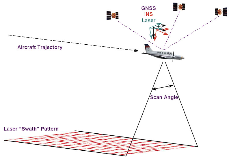
The use of a precise wide-area positioning technique for airborne trajectory solutions for LiDAR surveys provides both relative and absolute accuracies similar to those derived from using a local GNSS reference station.
Airborne light detection and ranging (LiDAR) surveys are among the most advanced means of producing high-resolution, accurate surface elevation models used for many applications in surveying and civil engineering. Precise geolocation and orientation (or georeferencing) of the LiDAR instrument with a combination of on-board GNSS and inertial sensors at the times when the measurements are made provides the key to high-quality elevation products.
The usual practice deploys reference GPS/GNSS land receivers in the area where the aircraft will be flying, to obtain a precise trajectory by short-baseline differential GNSS techniques. This could mean installing and operating receivers at many sites during a flight mission if the area surveyed is a large one.
We have tried a different approach: using as reference receivers those of a sparse network of Continuously Operating Reference Stations (CORS) in New South Wales known as CORSnet-NSW, and a wide-area differential GPS technique for obtaining the aircraft trajectory with sub-decimeter accuracy even with baseline lengths of several hundred kilometers. This may be comparable in precision and accuracy to the short-baseline method, but without the cost and logistical complications. This opens up a new level of operational capability, allowing flexibility for weather conditions and priority response applications.
The tests described here were organized and conducted by the NSW government’s Land and Property Management Authority, in collaboration with the University of New South Wales, in June 2009. CORSnet-NSW consists, at this writing, of 46 stations and by 2012 will provide statewide GNSS positioning infrastructure across NSW with a planned 70 stations in operation.
Precise Wide-Area Positioning
We used a technique for long-baseline differential, off-line positioning, able to deliver centimeter precision for fixed receivers and sub-decimeter precision for moving receivers. This choice was dictated by three considerations:
The intended application was the geolocation of the data of an airborne scanning LiDAR sensor to be used in the generation of high-accuracy digital elevation models (DEM).
Off-line processing, where all the GNSS data collected during the flight are available for processing and (as in this case) there is no need for immediate results, is intrinsically more reliable than real-time processing, where the data are available only up to the present epoch, and accurate results must be obtained right away, with no chance for a second try.
Differential processing makes it possible to resolve the carrier-phase ambiguities using well-understood methods.
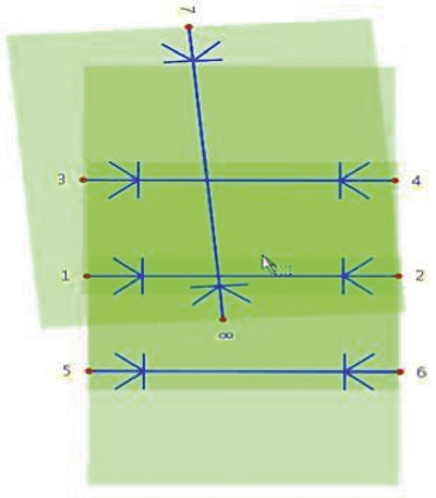
Technique. It is common practice in airborne LiDAR surveys to use GNSS both to position the instrument precisely, and to assist an inertial navigation system (INS) to obtain the orientation of the aircraft in space, as both position and orientation are needed to interpret the data properly. FIGURE 1 illustrates the relationship between the sensors used for airborne LiDAR surveys. The aircraft uses a GNSS antenna combined with an INS to georeference its trajectory. The bore-sight calibration process aligns the individual sensor orientations and standardizes the range measurements. However, if the survey is to achieve the now-expected high level of vertical accuracy (615 centimeters, 1 sigma), then the position of the GNSS/INS-derived aircraft trajectory for each laser swath must be determined with a relative precision in the order of just a few centimeters. This is achieved via differential GNSS post-processing of the kinematic airborne data together with static observations collected on precisely surveyed ground reference stations. The GNSS positions are then blended with high-frequency measurements taken by the onboard INS to produce the final trajectory and reference orientations.
Figure 1. Airborne LiDAR reference frame.
To such ends, the aircraft trajectory is usually determined by short-baseline differential GNSS, with ground receivers deployed near the intended flight path of the aircraft. In this way it is possible to use GNSS data analysis techniques that are both precise and quite straightforward to implement in software. The simplicity of these techniques is possible because, in short-baseline differential solutions, the data of the aircraft receiver and any nearby network receivers have much the same systematic errors (due to such things as satellite ephemerides errors, transmission delays, and so on) that cancel out — or nearly so — when their observations are differenced between them. This also makes it possible to resolve quickly and reliably the cycle ambiguities in the observed carrier phase, the most precise type of GNSS data, overcoming one of the main obstacles to obtaining good results. Furthermore, it is possible to get such results with single-frequency receivers, as ionospheric delay is one of the systematic effects that can be largely canceled out.
In wide-area solutions, those cancellations are not complete enough to ignore the systematic data errors, and they have to be included in the form of additional unknown parameters in the observation equations. Also, it is necessary to account for the ionospheric delays using dual-frequency data, which means using more expensive GNSS receivers and antennas.
Resolving the carrier-phase ambiguities is no longer straightforward or assured. The standard way of dealing with the ambiguities is to include them as unknowns in the observation equations and adjust them along with the other unknowns: this is often referred to as “floating the ambiguities.” Fixing (or resolving) those ambiguities to their most likely integer values in a matter of seconds to a minute is possible on occasion, when the aircraft is within less than 20 kilometers from a ground receiver, or very precise corrections for the ionospheric delay are available; otherwise slower techniques, that require tens of minutes, may be used. It is also necessary to correct as well as possible such things as the neutral atmospheric delay of the GNSS radio signals, the movement of the “fixed” stations due to plate tectonics, the solid earth tide using mathematical models, and, in the case of the tropospheric delay, estimating the error in the corrections made using a standard formula as an additional unknown per receiver.
Over the years all these difficulties have been gradually dealt with more effectively, more efficiently, more reliably and, from the user’s point of view, less painfully. Originally developed for the repeated determination of station positions to measure the slow tectonic deformations of the Earth’s crust, and to calculate precisely the orbit of Earth-observing satellites, these days, after nearly 30 years of steady progress, GNSS wide-area techniques and the corresponding software find many applications in science, engineering, and navigation, and are becoming widely used in remote sensing.
Software. We used the Interferometric Translocation (IT) wide-area positioning software developed by one of us for the long-baseline aircraft trajectory solutions and also to re-position in the IGS05 international reference frame some CORSnet-NSW stations, so their data could be used consistently in the differential wide-area solutions. These stations were originally given in the Geocentric Datum of Australia (GDA94). For both purposes we used the precise final GPS orbits computed and distributed by the IGS.
To validate the aircraft trajectories calculated with the wide-area method, we relied mainly on the quality of the LiDAR DEM results obtained with those trajectories. We also used commercial software to generate short-baseline differential solutions with receivers deployed near the intended aircraft flight-path, as is common practice in this type of survey, and compared them with the wide-area solutions (they turned out to be quite similar to short-baseline solutions obtained with the wide-area software).
Airborne Tests
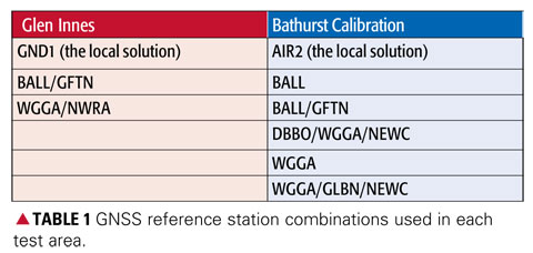
This study has used data from two airborne LiDAR surveys conducted by the NSW Land and Property Management Authority (LPMA) in June 2009. The first took place near the township of Glen Innes, and the second was a bore-sight calibration flight near the city of Bathurst. For both LiDAR surveys, the following data were acquired:
Aircraft trajectory, raw dual-frequency GPS (1 Hz) and IMU data (200 Hz).
LiDAR (raw return data for each laser pulse).
GPS reference station data from local receivers and multiple CORSnet-NSW sites.
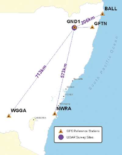
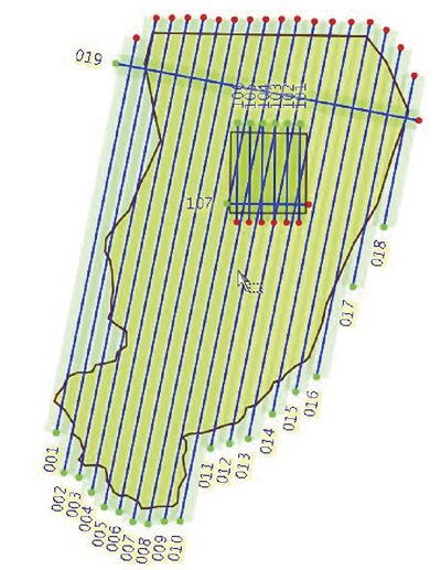
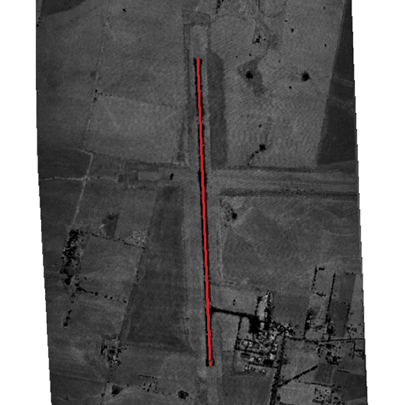
Glen Innes Test. This operational LiDAR survey established GND1 as the local reference station within the survey area. CORSnet-NSW data were collected for the test from GNSS receivers in Ballina (BALL), Grafton (GFTN), Nowra (NWRA), and Wagga Wagga (WGGA). FIGURE 2 shows the distribution of the reference stations and the flight runs.
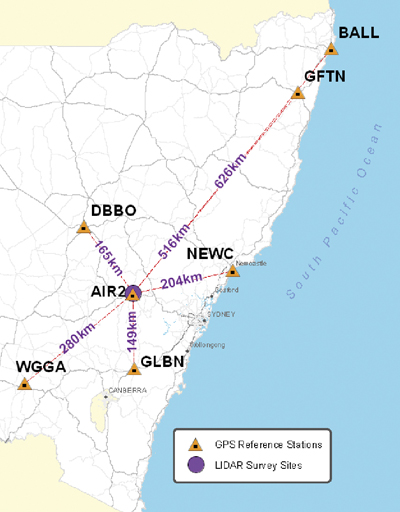
Figure 2. Glen Innes survey of June 9, 2009, showing the distribution of reference stations with baseline lengths and the survey area with (numbered) flight runs.Bathurst Test. Bathurst Airport is LPMA’s LiDAR calibration site and has various arrays of accurate ground checkpoints. AIR2, near the runway of the Bathurst airport, is the locally established GNSS reference station. CORSnet-NSW data were collected for the test from receivers in Ballina (BALL), Dubbo (DBBO), Grafton (GFTN), Newcastle (NEWC), Nowra (NWRA), and Wagga Wagga (WGGA). FIGURE 3 shows reference-station distribution and a schematic of the flight runs.
Figure 3. Bathurst test of June 16, 2009, showing the distribution of reference stations with baseline lengths and the survey area with (numbered) flight runs.
Effect on LiDAR Data
Rather than simply comparing aircraft trajectories, this study aimed to determine what effect the use of wide-area GNSS positioning has on the actual LiDAR point data and associated elevation surfaces. In terms of the horizontal accuracy required for LiDAR surveys, initial tests showed that the differences between the horizontal positions of various trajectories was negligible; therefore, only the vertical component was considered in this analysis.
To quantify differences between LiDAR data generated from trajectories using various combinations of distant GNSS reference sites, we applied four types of analysis:
Comparison of trajectories — directly compare the locally computed trajectory (assumed to be truth) with each wide-area derived trajectory.
Relative LiDAR point comparison — compare the positions for a sample of LiDAR ground points derived from the locally computed trajectory with those derived from each wide-area derived trajectory.
DEM comparison — difference the raster surfaces derived from the locally computed trajectory and a wide-area derived trajectory to find the effect over a LiDAR run.
Absolute LiDAR ground control comparison — compare the LiDAR derived surface from various trajectories to the surveyed ground control (Bathurst Calibration test site only). This also involves vertically shifting the resulting surface so that its offset relative to the one used as control is zero, thus removing the effect of using different reference frames for the GNSS trajectories and the control surface.
Trajectory Comparison
The comparison between the locally determined and each wide-area derived trajectory was made along the entire trajectory for each flight. The importance of this step lies in the assumption that all LiDAR data are directly positioned from the trajectory and so any systematic effect in the trajectory should be reflected on the ground. For each test site the locally derived solution is assumed to be “truth” with the vertical difference computed against wide-area solutions for each combination of reference stations used (TABLE 1).
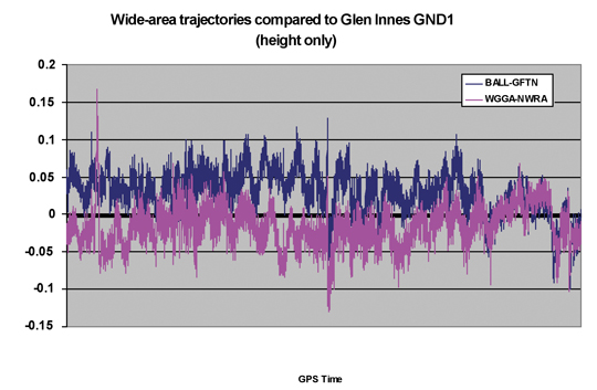
Glen Innes Test. FIGURE 4 shows the vertical comparison of two wide-area derived trajectories (using BALL and GFTN, and WGGA and NWRA, respectively) against the locally derived trajectory (using GND1). It can be seen that once the aircraft attained its stable operating altitude, the wide-area derived trajectories are generally within 5 centimeters of the locally derived solution.
Figure 4. Trajectory elevation differences for entire Glen Innes flight.
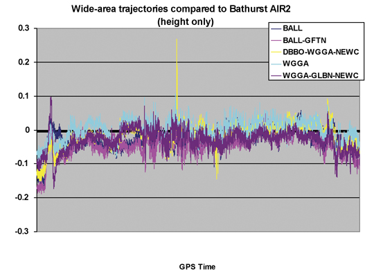
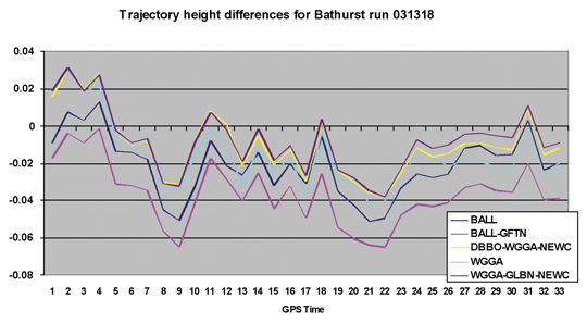
Bathurst Test. The Bathurst test differs from the Glen Innes test in that both the duration of the flight and the length of each run are significantly shorter. FIGURE 5 shows the vertical component of five wide-area derived trajectories, using several combinations of CORSnet-NSW reference stations, compared against the locally derived trajectory (using AIR2). The results once again show a remarkably consistent comparison with the locally derived solution. Data spikes showing up in the DBBO/WGGA/NEWC (yellow) solution were attributed to small data glitches at the DBBO CORSnet-NSW site. Unfortunately, LiDAR data were not collected at those instances; therefore, the effect on ground data could not be fully assessed.
Figure 5. Trajectory elevation differences for entire Bathurst calibration flight.
Relative Comparison
Regardless of the trajectory and orientation used to georeference LiDAR data, the same number of points will be created. It is therefore possible to create a LiDAR dataset using the same raw LiDAR data but different GNSS trajectories, and compare the results to determine the relative positioning differences on the ground.
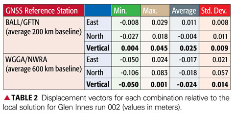
Given the large number (many millions) of points in a LiDAR dataset, we used a representative sample of evenly spaced 10 2 10 meter areas each containing 50–100 points (on level ground) for statistical analysis. We calculated displacement vectors between points computed from the locally derived trajectory and those using wide-area trajectories. Results from flight run 002 at Glen Innes (see Figure 2) and run 7 at the Bathurst Calibration test site (see Figure 3) are presented here.
Glen Innes Test Run 002. The displacement vectors from 46 sample areas (4,620 points) are summarized in TABLE 2, being points computed using the two wide-area solutions compared with the locally derived solution using reference station GND1. Note the high accuracy achieved in the all important vertical component.
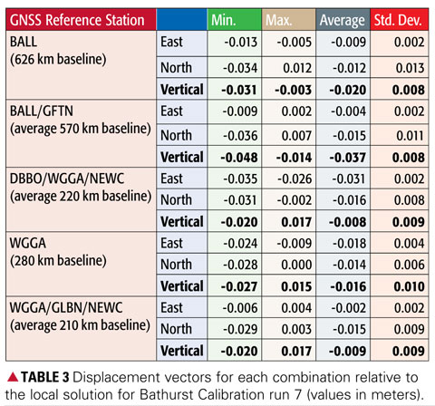
Bathurst Test Run 7. The displacement vectors from 25 sample areas (1,700 points) are summarized in TABLE 3, being points computed using the five wide-area solutions compared with the locally derived solution using reference station AIR2. Once again the results clearly show that the height values agree to within a few centimeters, even over baselines of more than 600 kilometers in length.
DEM Comparison
To investigate how the LiDAR surfaces derived from each trajectory compare across the entire data swath, we created raster surfaces from the LiDAR point data. Each surface was then subtracted from the local solution to create a difference surface. Visual inspection and interpretation was then used to discern any patterns or effects.
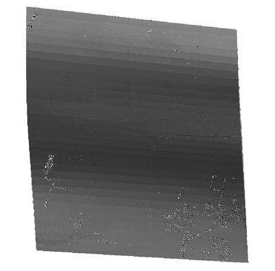
The result shown in FIGURE 6 (Bathurst Calibration flight run 7) was typical of the cyclical effect evident for all solutions. The magnitude of the difference was in the order of 2–3 centimeters and is in the direction of flight (north to south). If this cyclical variation is compared with the trajectory comparison for just the 33-second duration of flight run 7, a clear (expected) correlation with the variation in height is evident (FIGURE 7).
Figure 6. Subtraction surface for Bathurst Calibration run 7 (AIR2 vs. BALL).Figure 7. Trajectory comparison for Bathurst Calibration run 7 (031318).
No DEM comparison results are presented for the Glen Innes data because of significant variation in terrain and vegetation, making interpolation difficult and unreliable.
Absolute LiDAR Comparison
Ground control points serve two purposes in a LiDAR survey:
The calculation of statistics to describe vertical accuracy, that is, quantifying the match of the surface to the local height datum.
The calculation of a surface adjustment to enable transformation of the LiDAR points to fit the local height datum.
Additionally, ground control points with accurate heights are used to calibrate the sensor before use in active LiDAR surveys to account for internal electrical delays in the ranging and measurement system. LPMA maintains a calibration site at Bathurst Airport for this purpose, and regularly surveys the area to ensure the sensor is operating at maximum accuracy. It should be noted that the sensor was calibrated using Bathurst Airport ground control data prior to this study.
Surveyed Ground Control. The airport runway centerline vertical profile for the Bathurst Calibration site (FIGURE 8) was re-computed in terms of the same IGS05 reference frame determined for the LiDAR trajectories, thereby allowing an independent comparison with ground truth.
Figure 8. Runway vertical profile at the Bathurst Airport calibration site.
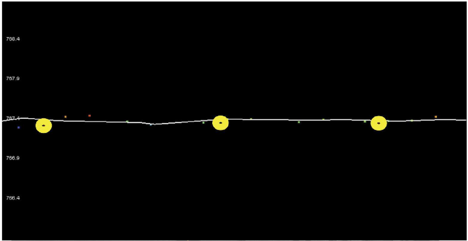
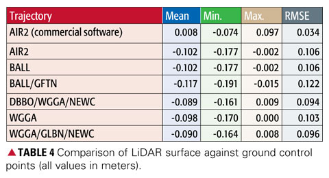
Point Comparison. Data from Bathurst run 7 were used to compare LiDAR results with the established ground control using a basic triangulated irregular network (TIN) surface comparison (FIGURE 9 and TABLE 4). In Figure 9, the TIN surface is indicated by the white line, while the ground control points are shown with yellow buffers.
Figure 9. Comparison of LiDAR surface and ground control points.
The first trajectory in Table 4 is the original calibration comparison using commercial software and orthometric height data. All wide-area solutions display a similar vertical offset, because of the use of different reference frames for the GrafNav and wide-area solutions (IGS05 vs. GDA94), and differences in the implementation in software of, for example, antenna corrections and atmospheric modeling. At first glance, the significant differences to the GrafNav trajectory caused the wide-area result to not satisfy the accuracy specifications for LiDAR. However, had the wide-area solutions been used for the sensor calibration, the figures would have been much closer to the ground truth.
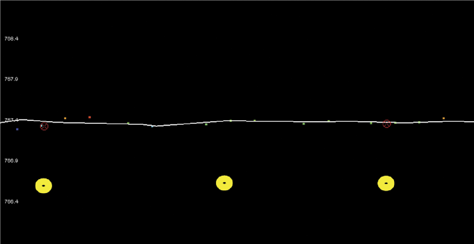
Block-Shifted Data Comparison. In an operational environment, because of systematic errors in the resulting DEM relative to the local height datum, this mean vertical offset is a common occurrence with comparisons against ground control similar to those shown in FIGURE 10. Again, the TIN surface is indicated by the white line, and the ground control points are shown with yellow buffers.
Figure 10. Usual operational comparison of LiDAR surface and ground control points.
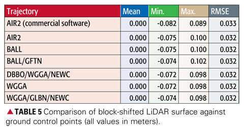
In standard LiDAR operations, the mean vertical offset between the initial results and the ground control, at the control points, produces a zero-mean offset. Following this procedure in this case results in the variation in the comparison of LiDAR data with ground truth now being well within the required limits of 615 centimeters (TABLE 5). The values show that after a block shift, trajectory solutions are virtually identical with a root mean square error of 32 millimeters. Thus, local GNSS reference stations can be replaced by distant CORS sites without loss of accuracy.
Conclusions
A precise wide-area positioning technique for airborne trajectory solutions provides both relative and absolute accuracies similar to those derived from usinga local GNSS reference station. Irrespective of which reference sites are used and once calibration and antenna modeling issues are addressed, the absolute comparison with ground control is well within the required accuracies. With the configuration of a GNSS network such as CORSnet-NSW (when complete, at least one site will always be within 150 kilometers of any point within New South Wales), an airborne LiDAR survey in the network’s service area can provide data for computation of an accurate sensor trajectory. This potentially negates the need to place and maintain ground reference stations close to the survey area — an exercise which not only requires significant resources but also reduces the operational flexibility of the aircraft.
The challenge for this technique in an operational environment is to define and maintain a precise reference frame for all CORSnet-NSW sites and observations, including the use of a stable ellipsoidal height datum with compatible geoid modeling in order to provide local orthometric elevation data. The knowledge base required for computation of wide-area GNSS solutions is significant and requires understanding of geodesy, GNSS positioning, absolute antenna modeling, application of precise ephemerides, and derivation of the other parameters inherent to successful ambiguity resolution over long distances.
Regardless of processing method, a LiDAR survey will always require independent ground surveys for collection of vertical checkpoints, which provide quality control to ensure the accuracy meets specifications, and the means to define any transformations necessary to fit LiDAR data with local height datum.
Manufacturer
NovAtel’s WayPoint GrafNav software was used for comparison purposes.
The ”IT” Software
Runs under Windows, Unix, Linux, and FreeBSD.
Source code compatible with most Fortran compilers.
Follows the IERS 2003 conventions.
Available mainly for collaborative research purposes, with a Free Software Foundation General Public Lice
nse.
Stop-and-go for rapid mobile surveys with pre-surveyed waypoints.
Differential, precise point positioning, mixed mode (precise differential + point positioning).
Data corrected for: Earth tide, neutral atmosphere radio signal delays, carrier phase windup, and so on.
Estimated parameters:
Receiver position in the IGS05 reference frame, with the WGS84 reference ellipsoid, earth spin-rate, light speed, GM constant.
Biases in ionosphere-free carrier-phase linear combination (“floated” ambiguities).
Neutral zenith delay correction error.
Broadcast orbit errors (allows precise differential near-real time solutions).
Integer ambiguity resolution available in differential mode, with short baselines up to 20 kilometers (in minutes), and baselines of unlimited length (in tens of minutes — or just minutes, with a precise ionosphere correction).
Oscar L. Colombo received a degree in electrical engineering from the National University of la Plata, Argentina, and a Ph.D. in electrical engineering from the University of New South Wales, Australia. He is an independent consultant.
Shane Brunker is an airborne LiDAR and imaging specialist working in a consulting capacity for specialized LiDAR survey company Network Mapping (United Kingdom).
Glenn Jones is a senior surveyor at the NSW Land and Property Management Authority in Bathurst, Australia.
Volker Janssen is a GNSS surveyor (CORS Network) in the Survey Infrastructure and Geodesy branch at the NSW Land and Property Management Authority in Bathurst, Australia. He holds a Ph.D. from the University of New South Wales.
Chris Rizos is head of the School of Surveying and Spatial Information Systems of the University of New South Wales, has a surveyor’s degree and a Ph.D. from the same university, and is an specialist in geodesy and GNSS positioning.
Earlier today (August 31), I conducted a webinar entitled “Solar Activity, SBAS and 24+3 GPS Constellation Updates.” Considering we only announced the webinar three weeks ago, we had a fantastic registration numbers, with more than 570 registered. Thank you for attending if you did. If you weren’t able to you’ll be able to download the presentation by registering here. After registering, you’ll be notified when it’s available for download (usually a couple of days after the webinar).
I had a lot of questions before and during the webinar. As customary, I’d like to address some of those as well as present the poll results here. First, the poll questions and results with accompanying pie charts to illustrate the results.
Poll #1: How concerned are you about solar activity affecting your GNSS operations?
Total votes: 157
Gakstatter comment: These numbers don’t surprise me. Personally, I probably fall in the “Somewhat” category, but my GPS/GNSS field work is pretty flexible so I can easily adjust without much inconvenience. However, if I had several crews using GPS/GNSS on a daily or near-daily basis or I had equipment relying on GPS/GNSS, I think I’d be in the “Very” category because the $$ impact would be much higher.
Poll #2: If it was available, would you be interested in receiving alerts/warnings of solar activity that may affect GNSS operations?
Total votes: 176
Gakstatter comment: I’m not surprised at these results either. When I initially considered this poll, I was thinking about asking which type of platform you would prefer to receive alerts/warnings with the choices being Droid app, iPhone app, Blackberry app, text message, e-mail, etc. If you have a preference on that, fire off a quick e-mail to me. Secondly, a few of you pointed out that NASA has an app for this, but keep in mind that the system I’m considering is focused specifically on high-performance/precision GPS/GNSS users, which would eliminate a lot of the baggage of the alert/warning systems available today. Poll #3: Do any of your GPS receivers use SBAS (WAAS/EGNOS/MSAS) as a primary source of corrections?
Total votes: 115
Gakstatter comment: Not much to say here except that a substantial number of commercial GPS users are relying on SBAS. This has definitely been the trend over the past five years.
Poll #4: Do you expect that the GPS 24+3 configuration will improve your GPS productivity?
Total votes: 172
Gakstatter comment: Like most of you, I have great expectations for the 24+3 configuration. While launching more satellites with L5 would be nice, that’s a long-term effort, whereas the 24+3 configuration is something we will benefit from in a few months and are seeing some marginal benefit now. In January 2011, once all the satellites have arrived at their destination slots, I’ll plot new visibility charts and see where we stand.
Following are some of the questions that were posed by the audience during the webinar: Question #1: The blueline ends in late 2009. Any information on up-to-date activity?
Gakstatter comment: This question was in reference to the Solar Cycle 24 prediction chart I displayed. The chart was probably small and difficult to read when displayed on your computer. Here’s a larger version of it. This was a chart released by the NOAA Space Weather Prediction Center in May 2009. Although sunspots don’t directly affect GPS operations, there is some relationship between sunspots and geomagnetic storms. Below it is an updated chart with actual values through the end of July 2010.
Question #2: What tools/online sites can be used to see if there is a TEC anomaly at a specified time, including “today”?
Gakstatter comment: There is a cool real-time chart of the U.S. on NOAA’s Space Weather Prediction Center website. There are other interesting charts on SWPC’s website like the 10-day trend chart. The JPL had a website that displayed a real-time TEC, but I just checked it and it hasn’t been updated since June. Another website to check is the National Satellite Test Bed that displays a real-time plot of the WAAS ionospheric grid points. Click here to view a global real-time (updated every 60 minutes) TEC chart of the world published by the Australian Space Weather Agency.
Question #3: What is better for a receiver, Differential GPS or dual frequency? Any references on this?
Gakstatter comment: With respect to performance during periods of heightened solar activity, definitely dual-frequency receivers. Although I don’t have a specific cite for you right now, there has been plenty written on this subject. Single frequency DGPS receivers are the most vulnerable during periods of heightened solar activity.
Question #4: Is the disruption in the sub-meter scale, single-digit meters, or tens of meters?
Gakstatter comment: It depends on the severity of the geomagnetic storm. During the worst times of the Oct. 2003 event, it was up to 25 meters. That order of magnitude would be rare. Remember, those events occurred in about four days over the 11-year cycle. I have some figures that relate TEC to position error, but I’ll withhold those until I’ve got a better understanding of how practical they are.
Question #5: Is there some type of notification system for GNSS users of major solar events? E-mail alerts? Twitter tweets?
Gakstatter comment: Following are instructions for signing up for the NOAA alerts/warnings. This is a good start. Stay tuned for my alert/warning system later this fall. Follow me on Twitter at http://twitter.com/GPSGIS_Eric
Following are detailed instructions for signing up for alerts:
-Click on Email products (under the Support Services menu on the left)
-Create an account if you don’t have one already (it’s free).
-Click on Subscribe
You don’t want to subscribe to everything. Here are the ones specific for GPS operations:
-Advisories/Space Weather Bulletin
-Geomagnetic Storm Products/(sign up for both Alerts and Warnings for K6, K7, K8, K9 events.
-For high latitude (55 degrees and higher) users, als
o sign up for Alerts and Warnings for K4 and K5 events.
Question #6: There is already an iPhone/iPod application that gives alerts of solar activity.
Gakstatter comment: Yes, I’m aware of the NASA app and there maybe others, but in my opinion they are too broad for high-performance/high-precision GPS/GNSS users. Personally, I don’t need to know about new sunspots and where they are located on the sun (although it’s cool to see in that app). I need to know when geomagnetic events are occurring that may interrupt or affect my GPS/GNSS fieldwork.
Question #7: Ouch, we’re at 59 degrees north, and 134 west. Seems like these problems are “picking” on Juneau.
Gakstatter comment: The good news for you is that Alaska has the most dense concentration of WAAS Reference Stations in the entire WAAS coverage area. Well, maybe not Juneau, but certainly “mainland” Alaska :-). Seriously, parts of Alaska produce the best WAAS accuracy due to the high density of WAAS reference stations.
Question #8: Will parts of BC, Canada, be affected by the SBAS outage?
Gakstatter comment: Not really, except that you’ll have one less WAAS GEO satellite in view for a month or so until PRN 133 is operational in November. I don’t think you’ll notice any change in performance. The exception would be if your receiver uses SBAS ranging. In that case, you’d be tracking one less satellite between the time that PRN 135 becomes unusable and the time PRN 133 becomes operational.
Following is an elevation plot of the current WAAS GEO satellites (PRN 135 and PRN 138):
Following is an elevation plot of only PRN 138. This is a possible scenario after PRN 135 is unusable in October 2010 and before PRN 133 is placed into service in November 2010.
Following is an elevation plot of PRN 138 and the new PRN 133 GEO which is expected to be placed into service sometime in November 2010.
Question #9: With the 24+3 configuration, is it that some sats were flying almost in tandem and they are spreading them out more?
Gakstatter comment: Yes, that is essentially what is happening. Some believe, including me, that a 24+6 configuration would be even better! But, one step at a time. I feel good that the U.S. Air Force is listening and responding.
I addressed many of the questions from the webinar. Some will take a little research on my side to answer properly. I should be able to address those in the mid-September newsletter. Thanks again to those who registered for the webinar. Feel free to send me an e-mail any time with comments, suggestions or questions.
You might have heard reports this week about a solar storm this week. This is part of the new solar cycle (Solar Cycle 24) that I’ve written about several times. I want to periodically touch on this subject as the solar activity is going to increase over the next few years, and if the solar activity (geomagnetic storms, not sunspots) is severe enough, it will have an effect on GPS accuracy and tracking. Here’s the scoop on this week’s solar activity.
First of all, I’ll let you in on a secret. I’m working on a new solar activity notification system specifically designed for GPS users. The problem is that people see reports in the mainstream media about solar activity and they automatically assume that it’s going to affect their GPS. Not all solar storms affect GPS; in fact only very specific ones (geomagnetic storms) of sufficient strength will affect GPS operations. I’m working on a notification system that will be tailored to both GPS L1 and GPS L1/L2 users (they are affected differently) so GPS users can have a reliable and specific source of information on solar activity without having to wade through the mainstream media noise.
Stay tuned for details this fall in this newsletter to learn more about my notification system and how to and access it. If you’ve ever used some of the GPS hardware/software products I helped design, you know my top priority is to make it easy to use and understandable.
This week’s event was probably the strongest geomagnetic storm of this solar cycle and of recent years (edit: actually, the storm in early April 2010 was a little stronger), maybe since late 2006. It will create some beautiful “northern lights,” but as strong as that may seem, it still wasn’t strong enough to elicit even a “cautionary” warning to GPS users (neither GPS L1 nor GPS L1/L2).
NASA video of sun’s activity on August 2, 2010
The last geomagnetic storm that adversely affected GPS users was in December 2006. It affected some GPS users for 10-15 minutes. For such a short time, most users would not notice or they might attribute it to a local system malfunction. By the time they investigate and reset the system, the event has passed and the user is back in operation. It was barely noticeable, if at all.
On the other hand, a severe geomagnetic storm such as the one that occurred in October 2003 can last for days and wreak havoc on precision GPS receivers. During extreme geomagnetic storms like that one, GPS accuracy suffers a lot, especially with GPS L1 users. During that event, simulations from the University of Calgary showed that WAAS maximum horizontal error (95th percentile) reached 25 meters while single baseline DGPS maximum horizontal error (95th percentile) reached 18 meters.
Dual-frequency users aren’t affected as much by extreme events but aren’t immune. Extreme events such as October 2003 can cause a loss of phase lock, especially with L2 on receivers that utilizing codeless and semicodeless techniques, which are virtually all of the dual-frequency GPS receivers on the market as of today.
For GPS users, nothing can be done to mitigate the effects of a strong geomagnetic storm. The next best step is to try to predict when they will occur so GPS users know what to expect. Fortunately, these storms are not common and scientists can reasonably predict when an event will occur.
There are some good websites to reference when checking up on solar activity. A great place for Europeans to do this is at the Royal Meteorological Institute of Belgium’s website. The U.S. National Weather Service also operates the Space Weather Prediction Center. The Australian Space Weather Agency operates a Space Weather Prediction Center, too. Also, note that for those users along the equator and at higher latitudes, your area is more susceptible to stronger geomagnetic storm activity.
The websites listed above are chock full of information and predictive systems on space weather. In fact, I believe it’s too much information for most GPS users to efficiently interpret. The goal with my new initiative is to provide GPS users with a quick summary so they are able to make informed decisions in a few seconds. Again, stay tuned this fall for the rollout.
Conference/Webinar Presentations
Between webinars and conferences, I’ve put together a fair number of Powerpoint presentations. I’m in the process of uploading many of them, some dating back years, to our website. Currently, I’ve uploaded ones that date back to April 2010. I hope you enjoy them.
The following presentations have all been converted to PDF format and are copyrighted. Feel free to incorporate them (or parts of them) into your documents if you like, just please remember to attribute each page you use to my name, Eric Gakstatter, and GPS World/Geospatial Solutions.
2010 (July San Diego, California) ESRI Surveying and Engineering GIS Summit luncheon keynote presentation: Get It Surveyed (GIS).
2010 (June, Seattle, Washington) Asia-Pacific Economic Cooperation meeting: Mapping and Surveying with SBAS+GPS.
2010 (June, Portland, Oregon) Webinar: GIS Mapping for Forestry, Agriculture, and Other Natural Resource Professionals.
Note that for the following webinar, you can also download an audio portion of the webinar free of charge by clicking here.
2010 (April, Phoenix, Arizona) GITA Annual Conference: How the Evolution of GPS is Transforming Surveying and Mapping (along with Pamela Fromhertz of NGS).
Part 1 – GNSS Mapping/Surveying Technology Update
2010 (April, Phoenix, Arizona) GITA Annual Conference: How the Evolution of GPS is Transforming Surveying and Mapping (along with Pamela Fromhertz of NGS).
Part 2 – Machine Control Using GNSS
2010 (April, Phoenix, Arizona) GITA Annual Conference: How the Evolution of GPS is Transforming Surveying and Mapping (along with Pamela Fromhertz of NGS).
Part 3 – Sub-Meter Mapping Using GPS
2010 (April, Phoenix, Arizona) GITA Annual Conference: How the Evolution of GPS is Transforming Surveying and Mapping (along with Pamela Fromhertz of NGS).
The field at Commonwealth Stadium in Edmonton, Alberta, recently received a CDN $2 million renovation. The old natural-grass field had become expensive to maintain properly, and the Grey Cup game, Canada’s Super Bowl, will be played at Commonwealth Stadium this year. The stage needed to be re-set.
Renovation required total removal of the existing medium and subgrade materials to a 1.2-meter depth. Wilco Contractors Northwest replaced the subgrade to a planarity or flatness tolerance of 3 millimeters over a 3-meter length. To achieve this precision, Wilco used a machine automation system on a Volvo G-960 motor grader fitted with a GPS receiver, and base station nearby. A second grader carried a robotic total station.
“We probably have a quarter-million dollars invested in this,” said Wilco President Art Maat. “The machine-control equipment pays for itself on an annual basis. It enables us to construct projects to tolerances that other contractors cannot match, even though they have the same big iron capabilities we do.”
Work began with removal of existing soil mixes, drainage rock, and subgrade clay. A bulldozer and the two motorgraders graded the subgrade to a 0.5 percent slope on both sides of the field’s center spine. The work included the D-shaped zone behind each goal post, created by a running track encircling the field. In all areas, the slope must be constant. “The problem is, how do you grade that half-circle?” said Maat. “Grader operators and surveyors want to work in straight lines or on rectangular grids. We use the geo-tracker, or robotic total station, to control the grader blade three-dimensionally. It is one step more accurate than a GPS system.”
Using the robotic total station involves entering a digital terrain model, called a TIN-file, into the grader’s onboard computer. The grader is fitted with a mast and prism, which has a fixed relation to the grader blade. The robotic total station can see the prism, read its 3D location, and communicate it back to the grader. The computer processes the differences between the actual blade location and the digital terrain model to control the blade.
The GPS-equipped grader did the rough grading at 20-millimeter accuracy, and the prism-equipped grader handled the fine grading at sub-centimeter accuracy. With final subgrade complete, Wilco dug trenches to install a drainage system, covered with a geotextile. Working in four lifts of 300 millimeters each, Wilco filled the excavation with coal bottom ash, a gritty product like playground sand. “We took the TIN file and offset the elevation by 300 millimeters at a time.”
Savings. The machine-control equipment saved Wilco $15,000–$20,000 on surveying, for 100 hours or more at $150 an hour for a crew. “The systems make our equipment 25 percent more efficient on low-tolerance sites such as fields and running tracks where grades are critical,” Maat added.
To test planarity, Wilco stretched a stringline over a 3-meter distance at many points on the field and measured with a Canadian dollar coin, a looney. If they could fit a couple of loonies under the string, they had found a low spot. If they could fit only one, the 3-millimeter tolerance had been met. “Our feedback from the consultants was that they had never seen a field prepared this well, with very little adjustment required. The slope of the field had to be 0.25 percent from the centerline spine to the sides. And the slope of the D-shaped areas behind the goal posts was exactly the same.”
Manufacturers
Wilco uses a Leica PowerGrade GPS/GNSS receiver, Leica Redline base station, Redline Power Tracker robotic total station, and Geo-Tracker.
I attended (and presented at) the 2010 ESRI Surveying and Engineering GIS Summit (SEGS) last week, as well as the ESRI International User Conference (UC). I’m telling you, if you’ve never been to the SEGS and UC, just treat yourself one time. Make a mini-vacation out of it. San Diego is a beautiful place to visit. The weather is always moderate with low humidity and warm temperature. It was a little cooler this year than years past, but still absolutely beautiful with tons of sigh-seeing. My wife has accompanied me for the past few years and she always enjoys herself and finds something new every year.
I believe that if you just go just one time, your vision of surveying, engineering, construction and GIS will change forever. I know it sounds like an advertisement from ESRI, but I think my pitch is even better than theirs :-). Seriously though, there are so many people presenting so many different ideas, and they are all related to the kind of geographic data you work with on a regular basis.
But, like anything else, it’s not all good. There are some drawbacks, so I’ve come up with my Good, Bad, Ugly list with respect to the conference. I think its pretty objective.
The Good
The single largest gathering (13,000+) of GIS, surveyors and engineers in the world (although one could argue that Europe’s INTERGEO might be larger).
A pre-conference (SEGS) that is designed specifically to cater to the land surveying and engineering folks.
Ideas and technology are presented that you will not find anywhere else.
The opportunity to network and collaborate with a large number of peers that you will not find anywhere else.
In 2011, the national ACSM (American Congress on Surveying and Mapping) conference will be combined with the SEGS.
San Diego is a beautiful city with beautiful weather and lots to do within walking distance of the convention center.
The Bad
Since it’s a vendor-specific conference, ESRI competitors such as Autodesk, Intergraph, etc., are not invited. In fact, if you tick them off, they might not invite you back next year.
A lot of time away from work during prime field season (July).
You could be overloaded if you aren’t prepared for the barrage of information and technology.
The Ugly
The whole experience isn’t cheap. The conference registration is expensive and San Diego is an expensive place to visit.
The San Diego airport is horrible, but at least it’s a very short ride to the convention center.
The Surveying and Engineering GIS Summit (SEGS) is held the weekend prior to the massive User Conference (13,000+ people).
I’ve heard rumblings about this for quite awhile. Here are my thoughts.
The ACSM national conference is dying and needed to do something drastic. This year, it co-located with the GITA (Geospatial Infrastructure Technology Association) national conference in Phoenix, Arizona, back in April. I attended that conference, too. Even though I was disappointed in the lack of coordination between the ACSM and GITA technical programs in Phoenix, the technical content was very good. Attendance, on the other hand, was horrible. It wasn’t sustainable from a business standpoint.
Because the annual ACSM conference was on a quick road to nowhere; it had to make a move to team up with another conference. Who?
The GITA conference dissed ACSM (or maybe the other way around) and is flying solo next year in Dallas, Texas. I think the attendance at the GITA conference will be a disaster. They already have a GITA Oil & Gas conference in Houston.
Another partner choice would be ASPRS, but for some reason, ACSM and ASPRS can’t figure out how to put something together even though the conferences were at the same time this year. Someone’s ego probably got bruised.
Partner with Autodesk? No way. Autodesk is a $2 billion behemoth. They don’t need or have the time to deal with ACSM.
That leaves the ESRI SEGS. Attendance-wise, the SEGS has been flat, or even lost ground. It needed a boost. Bringing in ACSM was a smart move, essentially increasing its attendance from 300 to 1,200. For ACSM, it wasn’t the ideal choice, but it was the only choice. It couldn’t afford another solo event in some off-beat city. The bottom line is that conferences need a healthy number of exhibitors and commercial sponsors in order to be financially viable. For companies to be interested there needs to be a healthy number of attendees. It’s a vicious circle. If attendance wanes, then exhibitors and commercial sponsors start to pull out.
Even though there is some pretty good upside for ACSM and ACSM membership in combining the conferences, I think the general ACSM membership will suffer. The primary reason is because it’s stuck in San Diego for the next three years. The U.S. Mid-Westerners and U.S. East Coaster’s will hesitate to make the trip due to the distance and expense of the conference, especially with the poor U.S. economy. I think what you’ll see are the state association conferences becoming stronger as they have been in the last few years. I wish, somehow, that some of the energy and excitement from the ESRI conferences could make their way to the state conferences.
I may sound wishy-washy, but in the final analysis, I think this is a good move. For ACSM, it was the only move and for ESRI, a feather in their cap. It’s interesting to note that even though it’s a three-year agreement, either can opt out annually.
On to the technical part of the SEGS conference
I blogged about the SEGS while I was in San Diego. Click here to view my summary.
A few of points I’d like to quickly emphasize:
Crowd-sourced data. There’s a lot of buzz about this, and rightfully so. SEGS keynote speaker Nancy von Meyer commented on crowd-sourced data and the challenge of “authenticating” it. Crowd-sourced, or third-part,y data is coming in a big way. You can choose to ignore it, but the smart people will take the time to understand it and use it when appropriate.
On a related point, a Community Basemap initiative was announced at the ESRI UC Plenary. The idea is that you contribute to the “community basemap” and, in return, you receive a better basemap than you started with. Granted, you have the same “data authentication” issues as crowd-sourced data, but if you understand it, there is value.
Imagery (e.g. ,satellite images, aerial photography). From following t
he satellite imagery vendors, I’ve known that imagery is progressing. Its quality (pixel resolution) and availability is improving. But, I’ll admit that I was taken back a bit when Lawrie Jordan, founder of ERDAS (he later sold to Leica) said this is the most exciting time in his 40-year career in imagery. He said that in less than five years, every square inch of the Earth will be constantly imaged by satellites. Now, ground truth accuracy is another story…
On Sunday, I made the keynote presentation during lunch. The title of my presentation was Get It Surveyed (GIS). The title was said tongue-in-cheek of course. There were many directions I could have gone, but I decided on three topics.
A GIS isn’t driven by spatial data accuracy.
GNSS technology in the next 10 years is going to advance significantly faster than the past 10 years.
The land surveyor’s role in the next 10 years is going to change significantly more than the past 10 years.
You may take offense to some of the details in #3, and I’m sure some of you did. I assure you, my intent was not to offend, but rather stimulate thought and consideration. Some comments I received after my presentation.
“You said what I’ve wanted to say, but can’t because my RPLS colleagues would kill me” (heard a version this from several people, two of whom are very prominent in the RPLS community).
“You are spot-on” (heard some version of this several times).
“Don’t forget about those who specialize in boundary surveys.”
“Your timeline of 10 years is too conservative; it will be more like five.”
A criticism I heard (not directly, but through the grapevine), was from someone who was particularly incensed by my presentation. I’m sure there were several people with this attitude. No doubt these criticisms are in reference to my thesis about land surveyors’ practices evolving and/or my comment that most RPLS’s aren’t qualified to manage a GIS. The criticism doesn’t surprise me. I’d be surprised (and probably disappointed) if it didn’t evoke any. Change doesn’t come easy and some will choose to give up rather than change.
No matter if you were at the live presentation or not, I’d love you hear your comments on it. You can download it by clicking here.
Lastly, during the Q&A after my presentation, I was caught flat-footed with a question about GIS licensure. I sort of stumbled and then stated that the technology is moving too rapidly and the bureaucracy of licensure couldn’t keep up. It didn’t take long for me to realize, and others to point out, that it wasn’t a very intelligent answer. Several people approached me afterwards and were able to express their opinions more eloquently and clearly. For what it’s worth, not one of them was in favor of GIS licensure. I will dedicate another article to this subject.
In closing, following are some photos I took at the SEGS. I hope you enjoy them.
Interesting slide from ESRI’s Brent Jones showing the attendance breakdown at the SEGS
Countries represented at the SEGS
Panel Discussion lead by ACSM’s Curt Sumner (Nancy von Meyer – VP Fairview Industries, David Cowen – NGA Committee Member, Wayne Harrison – President NSPS)
Thought-provoking slide from Brent Jones
Another thought-provoking slide from Brent
Opportunities for surveyors in GIS according to Brent Jones
I received some interesting e-mails and saw some web comments regarding my newsletter column a couple of weeks ago titled “What’s Going to Happen When High-Accuracy GPS is Cheap?” The comments ranged from “I don’t believe it’s going to happen” to “We’d better adapt to the changes in technology.”
One comment in particular had me thinking about the title of the original article. Looking back, perhaps I should have used the word “precision” instead of “accuracy” in the title of the article. Accuracy is a tricky subject and a subjective term. What’s accurate to one person may not be to another. Also, you may be precisely correct, but not very accurate at all.
The point of the commentor was that high-precision GPS equipment in the hands of the general public will create many problems. There’s no doubt that will happen. Is there going to be a new type of service that surveyors can market to in order to clean up the problems that are created? Probably, and quite possibly only a small percentage of today’s surveyors will be qualified to do this type of work. One’s ability to understand and work with spatial data will be critical in helping organizations solve geospatial data problems. Thus, the importance of data management knowledge and skills I’ve mentioned before.
Geodesy is going to play a big role in the future, regardless if you don’t believe in GPS precision becoming as cheap as I believe. One can’t argue that precision and accuracy are improving, and with that will come geodetic problems with legacy data that need to be solved. Just imagine an electric utility company with its entire distribution system in a GIS (or CAD) that’s been ammended many times over a 30-year period. Imagine the disparate data sources and wildly varying data accuracy in such a system.
Let’s look at two of the other comments I received. Please note I’ve paraphrased, and sometimes combined, comments for the sake of brevity:
“They thought EDMs, total stations and online GIS were going to change surveying too, but they really didn’t.”
EDM’s and total stations are complicated and complex instruments (not to say that GPS receivers aren’t). About 10 years ago when my eldest son was nine, I taught him how to map using RTK. Granted, he was a classic “button-pusher,” having no idea what the technology was doing, but he knew which buttons to push to map a soccer field. I taught him to do this in less than 15 minutes. There’s no way I could have taught him to map a soccer field using an EDM or a total station in that amount of time, even if I had a full day. The first difference between GPS and other mapping instruments: it’s very easy to learn and use.
This subject reminds me of a photo sent to me from Indonesia many years ago. A guy I knew was training a massive number of Indonesian (200+) foresters on how to use handheld GPS/GIS data collectors. They had little or no previous experience with GPS. He had an auditorium set up with a large projection screen. In one of his Powerpoint slides, he had a photo of a chimpanzee sitting next to a GPS receiver. His point was, of course, that anyone can be taught to map using a GPS receiver. At that time, equipment and software wasn’t as easy to use as it is today. For starters, one had to post-process GPS data to improve accuracy, but even then the point he was making was clear. The ending exercise for the class was to locate three $100 bills stashed separately somewhere in Jakarta using only GPS coordinates provided. I thought that was an ingenius way of keeping the class attentive.
Anyway, back to the topic.
There are several reasons one can’t view future high-precision GPS L1/L5 receivers the same as EDMs, total stations, or any other automated measurement tool. GPS is simply different and will have a much greater impact on the way surveyors and their clients work.
GPS receivers are orders of magnitude easier to use and more productive than any other surveying measurement tool in history.
GPS is a mainstream consumer electronic technology that is spurring a lot of innovation.
With L5, GPS technology will be very precise (horizontal and vertical) and very inexpensive.
For these reasons, I think you can view GPS L1/L5 receivers as game-changing and industry-altering technology. The combination of ease-of-use and low-cost will put high-precision GPS in the hands of everyone from the garbage collector to the policeman mapping accident scenes. That wasn’t the case with EDMs, total stations, or any other measurement technology.
“Consumer-grade GPS receivers and survey-grade GPS receivers are not the same quality and never will be.”
This isn’t the case according to several GNSS receiver designers I’ve spoken to. There’s no reason a “consumer-grade” L1/L5 GPS receiver can’t achieve cm-level precision (horizontally and vertically) with a good quality antenna. Of course, it will need a source of correction, but in the 5-10 year window, RTK corrections will be more available and less expensive than they are today. The RTK corrections will likely be free so the only expense will be the wireless data plan.
There will be dozens, maybe hundreds of GPS chipsets designed for L1/L5. Many will be open systems where companies will be able to load their own firmware into the receiver to add specific features (e.g., more robust ambiguity resolution for surveying). The baseline L1/L5 GPS receiver may be only a few hundred dollars, but a customized version for specific applications will have a premium of a few hundred, or maybe $1,000+. For example, a GPS L1/L5 receiver that also includes Galileo signal and is customized for machine control with specific features might be $1,500. Commercial users will pay that premium. They already justify paying tens of thousands of dollars for the same performance today. The difference is that a low price point will attract a much larger audience.
There’s no doubt that there will be boutique, niche GPS L1/L5 receivers that will be able to garner a premium price, but surely the days of many thousands of dollars for high-precision GPS receiver are heading to an end.
This is not the end of land surveying. I didn’t claim it before and I don’t claim it now. That idea is ludicrous. But, you have to ask yourself how much time you spend on projects that will be affected by this technology.
If 75% of your work is boundary surveys, perhaps you won’t be concerned as much as the company that generates 75% of its revenue from construction work or topographic surveys.
If 75% of your work is mortgage surveys, you’ve got more to worry about than high-precision GPS. :-)
My point is that change is inevitable and that people who have the attitude that this is just another Chicken Little call (the sky is falling!) will be in for a rude awakening when the rubber hits the road. We can have a friendly debate about when this will happen, but there’s absolutely no doubt that it will.
Free Webinar on June 24
On June 24, Geospatial Solutions will be conducting a free 60-minute webinar, moderated by me, on “GIS Mapping for Forestry, Agriculture, and Other Natural Resource Professionals.” I will discuss GIS mapping software tools/concepts/techniques as well as GIS mapping hardware such as GPS receivers, digital cameras, and laser rangefinders. Although focused on natural resources, it will be relevant for all pe
ople interested in GIS mapping, which could be utility companies, municipalities, transportation organizations, etc. Sign up now by clicking here and submit questions in advance.