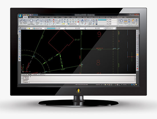
MicroSurvey Software has released MicroSurvey CAD 2016, the newest generation of its desktop survey and design program for land surveyors and civil engineers. Powered by a new IntelliCAD 8.1a engine and enhanced with a suite of new point-cloud management tools, the software makes high-impact drafting and design fast and intuitive, the company said.
Users on multi-core computers will experience up to 300 percent faster performance compared to previous versions, which substantially improves productivity. Navigation has been enhanced through a new ribbon interface with high-resolution icons that provide easy access to frequently used tools. The newest version of the software is also able to open and export DGN files, handle annotation scaling, and publish drawings as DWF/DWFX, PNG and JPG files.
Point Clouds. The new release includes significant enhancements for working with point clouds. The Ultimate and Studio versions of the software are now powered by the same point-cloud engine that drives Leica Cyclone and CloudWorx software, making it possible to directly import Leica Cyclone and Leica JetStream databases using Cyclone dialogs.
Users can view panoramic photographs captured by the laser scanner and snap to points directly from the photographs in a TruSpace window. Point-cloud data is now displayed directly within the CAD model space, and users can snap to the point-cloud points using standard CAD tools.
MicroSurvey CAD is compatible with field data from all major total stations and data collectors and is fully compatible with AutoCAD. It includes complete survey drafting, COGO, DTM, traversing, volumes, contouring, point-cloud manipulation and data-collection interfacing. No plug-ins or modules are necessary. Both a 64-bit version and a 32-bit version of the software are available.
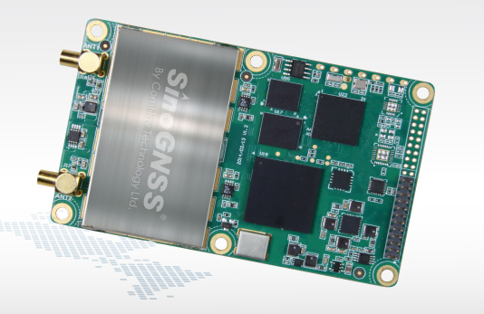
Positioning and heading for mission-critical applications
The K528G dual-frequency, multi-constellation GNSS board provides the highest accuracy in differential positioning. It benefits from numerous constellation signals because of its advanced tracking performance of both GPS and GLONASS. The K528G can provide positioning and heading information generated by two antennas. It is designed for guiding and positioning construction engines, dredges, barges, shipping container cranes, mining equipment and intelligent transportation systems.
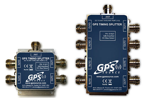
Designed for small-cell and distributed antenna systems
GPS Source has released of a line of GPS/GNSS splitters created for the small-cell wireless and distributed antenna system markets. Specifically designed for the L-band frequency, they can eliminate the cost of multiple antennas and long cable runs in wireless installations. With four or eight outputs, the new line of splitters make it possible to use a single GPS referencing antenna and cable arrangement for multiple synchronized systems. The splitters include features such as DC bias select and amplification. GPS Source RF signal splitters typically operate in conjunction with an active GPS antenna; consequently, a GPS RF signal splitter must have provisions for managing the DC voltage to the active GPS antenna. The S14GT and S18GT splitters will power an external GPS antenna from any of the RF outputs. A “hunt-and-pick” circuit is used to select only one DC input for power should more than one source be connected. Designed for redundancy, if the selected DC bias input should fail, the DC bias will automatically switch to another DC input to ensure an uninterrupted power supply to the active antenna.
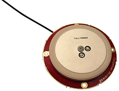
For precision industrial, agricultural and military OEM applications
A new series of L1 band wideband antennas for OEM applications is offered in three formats:
▪ TW2106/TW2108 — GPS L1
▪ TW2406/TW2408 — GPS + GLONASS
▪ TW2706/TW2708 — Galileo, BeiDou, GPS + GLONASS
Each antenna type features Tallysman’s Accutenna technology, which provides high rejection of multipath signals, with low axial ratios and tight phase center variations (PCV). Each is available with a brickwall pre-filter option to protect against saturation by high level subharmonic and L-band signals. The antenna printed circuit boards (PCBs) are 56 millimeters in diameter with four plated holes for secure mounting. They are available with a variety of connectors and custom cable lengths, and can be custom-tuned. All of them are REACH and ROHS compliant.
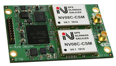
The NV08C-RTK-A is fully integrated multi-constellation L1 heading receiver with embedded real-tiime kinematic (RTK) functionality and compatibility with GPS, GLONASS, Galileo and BeiDou. The NV08C-RTK-A is designed for use in high-accuracy applications that demand low-cost, low-power consumption, a small form factor and high performance, such as construction, mining and industrial; environmental and structural monitoring; machine control; parallel driving systems; precision agriculture; UAVs; and robotics and intelligent machines.
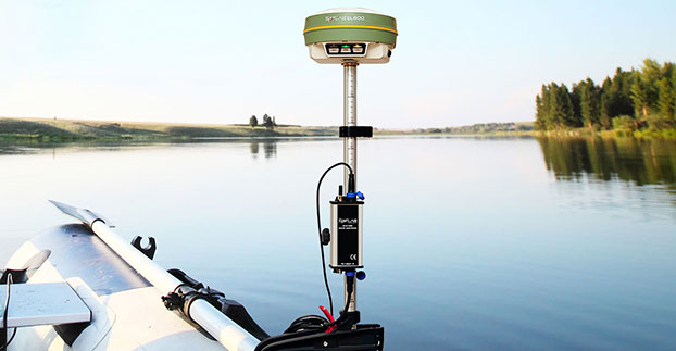
The SLD-100 GNSS Rover accessory facilitates hydrographic measurement in bodies of water up to 100 meters in depth. it is designed for anyone who finds themselves needing to survey into bodies of water, streams and rivers. With survey-grade accuracy, the SLD-100 can be added to any brand GNSS RTK rover to allow for position and depth measurements to be made simultaneously. With a built-in 10-hour lithium battery and transmitter unit with Bluetooth connectivity, the SLD-100 provides standard-depth data streams in several industry-standard NMEA formats at 1 Hz, 4800 bps, providing compatibility with any hydrographic surveying software package. Position and depth information is externally logged on a computer or controller. Included transom mounting hardware enables easy installation.
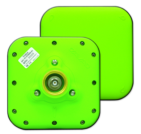
TriAnt is small, thin and rugged high-performance GNSS antenna. It measures 128 x 128 millimeters (mm) square and 39 mm thick. It can be mounted with three screws to flat surfaces. It is designed for applications such as machine control and surround anennas of the TRIUMPH-4X. The antenna cable is routed through the center of the antenna (TNC connector) for protection in harsh environments. The TriAnt can also be mounted on poles (1–14 inches thread) using its mount-pole attachment, which increases the thickness to 54.5 mm.
The X20i L1 GPS receiver by CHC Navigation is powered by a high-precision L1 GPS engine. Its integrated Bluetooth chip enables it to wirelessly collect submeter positions in real- time or centimeter post-processed on an iPhone or iPad. All location-aware apps on the iPhone and iPad are compatible with the X20i. Immediately after pairing and answering the security question allowing the X20i to take control of location services on the iOS device, 1 million iOS applications are capable of utilizing the high-accuracy data of the X20i, and become accurate to either 1 foot or 1 centimeter. Apps that can make use of the high accuracy include TerraGo Edge, ESRI’s ArcView Connector and those by CarteGraph Systems.
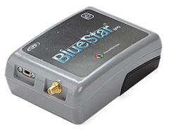
BlueStarGPS offers both GPS and GNSS options in a rugged, lightweight package. The BlueStarGPS device was designed to meet sub-meter mapping and data-collection needs in the pipeline and utility industries. It provides sub-meter precision without post-processing, and maintains accurate positioning when the SBAS signal is obstructed. This means it can function under trees, around buildings and in rugged terrain where other receivers can fail. The BlueStarGPS is designed specifically for use with Android mobile devices, such as smartphones, tablets or notebook computers, as well as cable and pipe “locating” tools with a connectivity range of up to 1 kilometer.
UAV measures through water surfaces of rivers, lakes
The RIEGL BathyCopter is a small-UAV-based surveying system capable of measuring through the water surface. It’s suitable for generating profiles of rivers or water reservoirs. The platform design integrates a topo-bathymetric green laser depth meter, an APX 15 inertial measurement unit (IMU)/GNSS with antenna, a control unit and a digital camera. Applications include generation of river profiles, survey of reservoirs and canals, landscaping, support of construction projects, and surveys for planning and carrying out hydraulic engineering work.
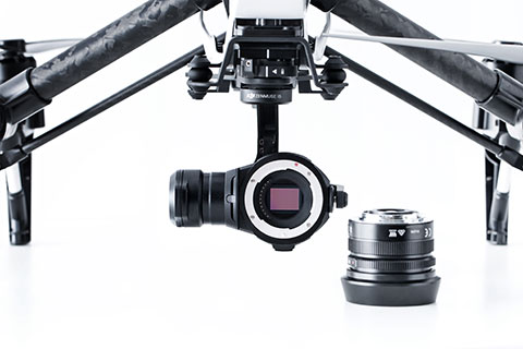
The Zenmuse X5 is a micro four-thirds (M4/3) camera designed specifically for aerial use. With a large sensor, aerial image makers will be able to capture up to 13 stops of dynamic range, enabling capture of high-resolution 16-megapixel photos or 4 k, 24 fps and 30 fps videos in complex lighting environments. It supports four interchangeable lenses. The Zenmuse X5 is designed for creation of high-quality aerial maps and 3D models, industrial and utility inspection, and professional video capture.
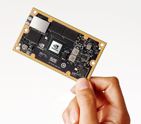
The NVIDIA Jetson TX1 module is designed to power smart devices — including drones that don’t just fly by remote control, but navigate their way through a forest for search and rescue. It is an embedded computer designed to learn to recognize objects or interpret information, incorporating capabilities such as machine learning, computer vision and navigation into a single system. This technology expands the ability of machines to operate on their own and adapt to their surroundings by recognizing images, processing conversational speech, or analyzing a room full of furniture and finding a path to navigate across it.
Part 1 of this series appeared in the June Survey Scene newsletter, Part 2 appeared in the August newsletter, and Part 3 appeared in the October newsletter. Upcoming Survey Scene newsletters will carry additional columns in this series.
Basic Procedures and Tools for Ensuring GNNS-Derived Ellipsoid Heights Meet the Project’s Desired Accuracy
David B. Zilkoski
In Part 1 of this series, I discussed the basic concepts of GNSS-derived heights; the article discussed the three types of heights involved in determining GNSS-derived orthometric heights: ellipsoid, geoid, and orthometric.
Part 2 discussed guidelines for detecting, reducing, and/or eliminating error sources in ellipsoid heights. It focused on guidelines for establishing accurate ellipsoid heights in a local geodetic network. It discussed procedures that need to be followed to detect, reduce, and/or eliminate error sources to estimate accurate GNSS-derived ellipsoid heights, and procedures for evaluating published NAD 83 (2011) ellipsoid heights.
Part 3 in this series described the differences between a scientific gravimetric geoid model and a hybrid geoid model, and why it is important to use both geoid models in your analysis. It highlighted that the latest published United States National Geodetic Survey (NGS) hybrid geoid model, Geoid12B, is made consistent with the United States national vertical height reference frame, that is the North American Vertical Datum of 1988 (NAVD 88). It emphasized that this means a user will be consistent with NAVD 88 when using GEOID12B to estimate GNSS-derived orthometric heights, but it doesn’t guarantee that your GNSS-derived orthometric heights are accurate. It demonstrated how to use these geoid models and ellipsoid heights to identify potential issues with published NAVD 88 heights.
This column (the fourth in this series) will focus on basic procedures and tools that should be used to establish accurate GNSS-derived ellipsoid heights for a project. It will provide basic procedures for ensuring a project’s GNSS-derived ellipsoid heights are meeting the desired accuracy. The accuracy of the adjusted ellipsoid heights must be evaluated first, so if there is an issue with the difference between the GNSS-derived orthometric height and published NAVD 88 height, the user will know if the ellipsoid height or the orthometric height is the problem.
NGS has developed guidelines that address the establishment and densification of vertical control networks through the use of GNSS surveys and valid NAVD 88 orthometric control. NGS has documented these procedures in NOAA Technical Memorandum NOS NGS-59, titled “Guidelines for Establishing GNSS-derived Orthometric Heights (Standards: 2 cm and 5 cm). The document provides basic rules and procedures that need to be adhered to for computing accurate NAVD 88 GNSS-derived orthometric heights. However, before we can validate NAVD 88 height constraints used to estimate GNSS-derived orthometric heights, we first need to ensure that the GNSS-derived ellipsoid heights are accurate to the desired requirements. It is impossible to describe all situations in a short newsletter, so this column will address the basic procedures with a few caveats.
Validating Your GNSS Survey Project’s Ellipsoid Heights
Part 2 discussed guidelines for detecting, reducing and eliminating error sources in ellipsoid heights (NGS 58). It focused on evaluating published NAD 83 (2011) ellipsoid heights. This column will discuss a few basic procedures for analyzing a GNSS project’s data to ensure the desired ellipsoid height accuracy standard has been met.
GNSS data can be evaluated by analyzing repeat baseline differences, network loop closures and residuals from a minimum-constraint least-squares adjustment. It was noted in the second article that if GNSS users follow the NGS guidelines, they will reduce and/or eliminate errors in ellipsoid heights and, at a minimum, they will detect problems or errors in data. It was also mentioned that the basic concepts are very simple, but they all need to be followed exactly as prescribed. For example, “the observing scheme for all stations requires that all adjacent stations (baselines) be observed at least twice on two different days and at two different times of the day.”
GNSS can provide “absolute” and relative positioning information much easier, faster and more precisely than some classical techniques. However, the wrong station can still be occupied, the height of the antenna can be measured wrong or incorrectly entered during the baseline reduction processing phase, the receiver can malfunction, an abnormal atmospheric condition can cause large errors in the height component, or some “unknown Gremlin” can be causing an error source.
Classical techniques of establishing horizontal and vertical control used networks that consisted of many loops, triangles and braced quadrilaterals. This design provided enough redundant observations to detect data outliers. NGS guidelines for establishing GNSS-derived heights were designed with this same concept in mind. Since all baselines must be repeated and adjacent station observed, analyzing repeat baseline differences, loop closures and residuals from minimum-constraint least-squares adjustments are very effective analysis tools for detecting data outliers.
Comparing Ellipsoid Height Differences from Repeat Baselines
This procedure is very simple: subtract one ellipsoid height difference from another, for instance, the ellipsoid height difference from baseline A to B on day 1 minus the ellipsoid height difference from baseline A to B on day 2. If this difference is greater than 2 cm, one of the baselines must be observed again. Comparing ellipsoid height differences from repeat baselines is a very simple procedure, but it’s also one of the most important. Many users complain about having to repeat baselines, but requiring an extra occupation session in the field can often save many days of analysis in the office. In addition, repeating the baseline provides the redundancy necessary to obtain the desired relative accuracy of the survey (that is, repeat measurements help to derive a more accurate result than a result derived from a single measurement).
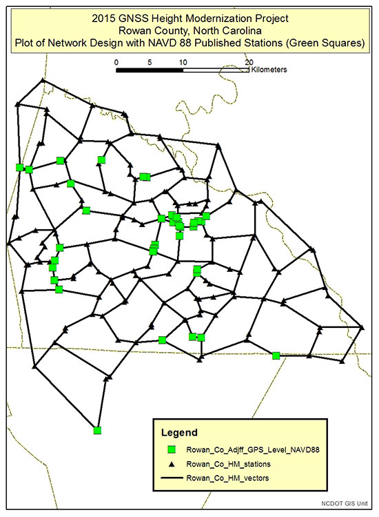
Figure 1 depicts the network design of a 2015 North Carolina Geodetic Survey (NCGS) GNSS Height Modernization Project. The data from this GNSS project was provided to me by the North Carolina Geodetic Survey (James G. Gay, chief of Western Field Operations, North Carolina Geodetic Survey, Division of Emergency Management/Risk Management, North Carolina Department of Public Safety, 2090 US 70 Highway, Swannanoa, NC 28778). It should be noted that these results should be considered preliminary and have not been finalized by NCGS personnel. This is an excellent example of a GNSS project that followed the guidelines outlined in NGS 58. The network design includes short baselines with many loops. The average length of baselines is 2.9 km, the maximum baseline is 13.5 km, and there are 465 baselines connected to 182 stations. All baselines were repeated, making the analysis easy.
Figure 1. Plot depicting the Network Design of the NCGS Rowan County Height Modernization GNSS Project.
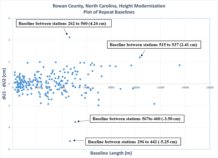
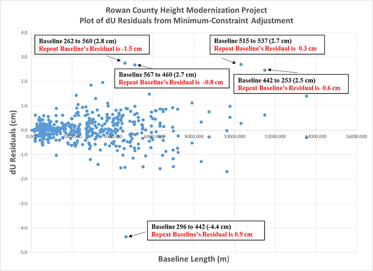
Figure 2 is a plot of the differences between repeat baselines. First, it should be noted that most baselines are less than 5 km and most repeat baselines differences are less than +/- 2 cm. There are some outliers, which is not unusual when performing GNSS surveys even when following all guidelines outlined in NGS 58. What is important is that these outliers are identified, and then additional observations are performed to meet the guidelines and obtain the desired accuracy of the survey.
The repeat baseline procedure helps to identify these outliers such as the baselines highlighted in figure 2. As noted in figure 2, the largest outliers are on two different baselines. These baselines should be re-observed to meet the NGS 58 guidelines. The requirement is to repeat the baseline on different days and at different time of the day. The reason for the requirement is to get two observations under different conditions and different satellite geometry. The user needs to determine which baseline is the outlier so he can ensure that he has two baselines with different satellite geometry. When a network is properly designed with short baselines and many loops, the results from a minimum-constraint least-squares adjustment can help identify the outlier.
Figure 2. Plot of repeat baselines for the NCGS Rowan County Height Modernization GNSS Project (does not include re-observations of repeat baselines that did not meet the 2 cm guideline).
Analyzing Loop Closures
Loop closures can be used to detect “bad” observations. If two loops with a common baseline have large closures, this may be an indication that the common baseline is an outlier. The following statement appeared in Part 2: “Please be aware that repeatability and loop closures do not always disclose all problems, and that is why it is important to adhere to the procedures outlined in NGS’ publications.” So why is it okay to use loop closures now?
Since users must repeat baselines on different days and at different times of the day, there are several different loops that can be generated from the individual baselines. If a repeat baseline difference is greater than 2 cm, then comparing the loop closures involved with the baseline may help determine which baseline is the outlier. As previously stated, according to NGS 58 guidelines, if a repeat baseline difference exceeds 2 cm, one of the baselines must be observed again, and baselines must be observed at least twice on two different days and at two different times of the day. If it can be determined which baseline is the potential outlier, the user will know which time of the day to re-observe the baseline. Therefore, loop closures can be very helpful in isolating errors when the user followed all of the guidelines outlined in the NGS 58 document.
Plotting Ellipsoid Height Residuals from Least Squares Adjustments
It is important that during the analysis of the GNSS-derived ellipsoid heights, the user performs a minimum-constraint least-squares adjustment and identifies potential outliers. This ensures that the GNSS-derived ellipsoid heights meet the user’s desired standards. This is not a complex procedure if the user knows how to perform a least-squares adjustment of GNSS data. Explaining least-squares adjustments is beyond the scope of this column. Today, most GNSS manufacturers provide support software that includes performing least-squares adjustments. NGS also provides software tools for validating data formats and performing adjustments. These tool can be found here. I used these tools to analyze and adjust the survey data of the Rowan County GNSS Height Modernization Project.
If users follow NGS guidelines and evaluate all repeat baselines, the adjustment results should confirm what has already been determined. For example, if a repeat baseline indicates a large difference between two vectors, then typically one of the residuals of one baseline should be larger than the other. Following NGS guidelines usually provides enough redundancy for the adjustment process to detect outliers and usually apply the residual to the appropriate observation, that is, the bad vector.
Like comparing repeat baselines, analyzing ellipsoid height residuals is also important. During this procedure, the user performs a 3D minimum-constraint least-squares adjustment of the GNSS survey project (constrain one latitude, one longitude and one ellipsoid height), plots the ellipsoid height residuals, and investigates all residuals greater than 2 cm.
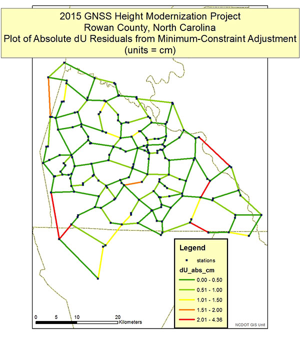
Figures 3 and 4 depict the dU residuals from a least-squares adjustment of the Rowan County Height Modernization Project. NGS’ adjustment program provides the vector residuals in dX, dY and dZ; and dN, dE and dU (local geodetic horizon coordinate system). dU residuals are not the same as dh residuals, but for all practical purposes can be analyzed just like dh residuals. Looking at Figures 3 and 4, a few items should be noted. First, all dU residuals are less than 2 cm except for five baselines. Four of the five baselines had repeat baselines that exceeded the 2 cm repeat baseline requirement (see Figure 2). For example, the plot of repeat baseline differences indicated that baseline between station 296 and 442 disagreed by 5.25 cm (see Figure 2). The plot of dU residuals (Figure 4) from the least-squares adjustment shows that one of the baseline’s residual is -4.4 cm and the other is 0.9 cm. The adjustment results are indicating which baseline needs to be re-observed to meet the guideline’s requirement of repeat baselines on two different days at two different times of the day. That’s all there is to it, when the user follows NGS guidelines exactly as prescribed.
Figure 3. Plot depicting absolute dU residuals from the NCGS GNSS Height Modernization Project (does not include re-observations of repeat baselines that did not meet the 2 cm guideline).Figure 4. Plot of all residuals from the NCGS Rowan County GNSS Height Modernization Project (does not include re-observations of repeat baselines that did not meet the 2 cm guideline).
The reader may have noticed that one large residual on the residual plot, baseline 442 to 253 (11.5 km), did not show up as a large different on the repeat baseline plot. There are several reasons why this could occur. For example, the stations involved in the baseline are not adjacent stations, so the baseline wasn’t repeated; the repeat baseline closure was large, but not greater than 2 cm; or the pair of stations are involved with many vectors and the one vector is inconsistent with the other vectors. Regardless of the reason, if there’s enough redundant observations to and from a station and the repeat baselines don’t indicate a problem, then the adjustment is doing what it’s designed to do; that is, detecting outliers and reducing their influence on the final adjusted height. In this particular case, the repeat baseline closure between stations 442 and 253 was 1.84 cm, which meets the NGS 58 guideline of 2 cm. The adjustment uses all of the data to determine the best set of coordinates. Based on the repeat baselines and loops surrounding the two stations, the adjustment indicated that one of the vectors fits better with the other vectors surrounding the two stations. Per the requirement of NGS 58 guidelines, the NCGS re-observed all five baselines with large residuals.
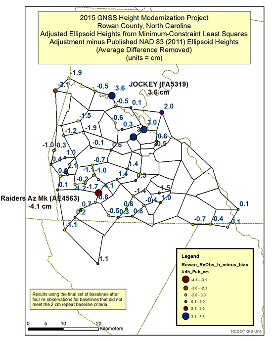
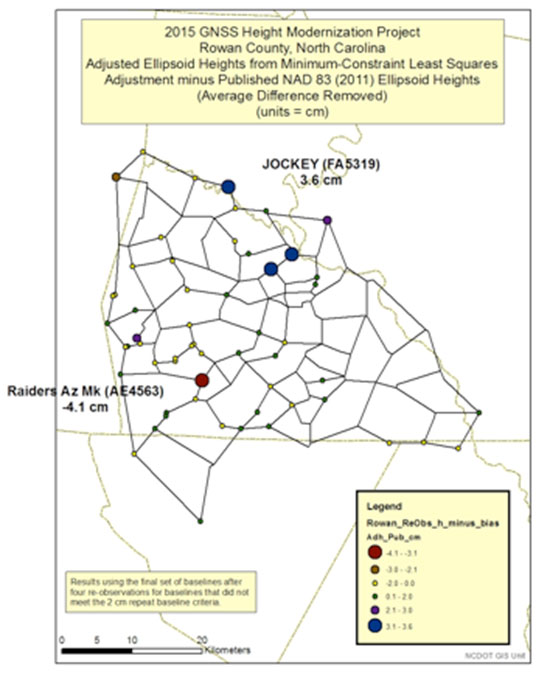
After all outliers are detected and removed from the adjustment, the user should compare the adjusted ellipsoid heights with the latest published ellipsoid heights, that is, NGS published NAD 83 (2011) ellipsoid heights. Figures 5 and 6 are plots of the adjusted ellipsoid heights from a minimum-constraint least-squares adjustment minus the NAD 83 (2011) ellipsoid heights. Since this was a minimum-constraint adjustment (that is, only one latitude, one longitude and one ellipsoid height value were constrained), a bias shift based on the average differences was removed from all differences. Most of the differences agree within +/- 2 cm. There are several that are greater than +/- 2 cm, but only one is greater than +/- 4 cm.
As mentioned in Part 2, many of the older GPS survey projects that were part of the NAD 83 (2011) network adjustment were not Height Modernization projects and were not performed following the NGS 58 guidelines. That is, most baselines are greater than 10 km and were not repeated. Therefore, in my opinion, many of the published ellipsoid heights local-height accuracies may be optimistic. The user should consider this when determining whether their results are more accurate than the published values. NGS’ Constrained Adjustment Guidelines for incorporating GNSS project data into NAD 83 (2011) state, “As a general rule, if the adjusted values of the constrained coordinates of a station shift by more than 2 cm horizontally and/or 4 cm in height, its horizontal coordinates and/or ellipsoid height, respectively, should be unconstrained.”
The stations that have height differences greater than 4 cm should be investigated. In addition, stations that have large relative height differences (greater than 4 cm) between closely spaced neighbors should also be investigated. For example, station Jockey’s difference is 3.6 cm, and two of its neighbors’ differences are only -0.5 cm. The relative difference exceeds 4 cm [3.6 cm – (-0.5 cm)] between two closely spaced stations.
Figure 5. Plot of adjusted ellipsoid height minus published NAD 83 (2011) Ellipsoid Heights (the number is the difference for that particular station; units = cm).Figure 6. Plot of adjusted ellipsoid height minus published NAD 83 (2011) published heights.
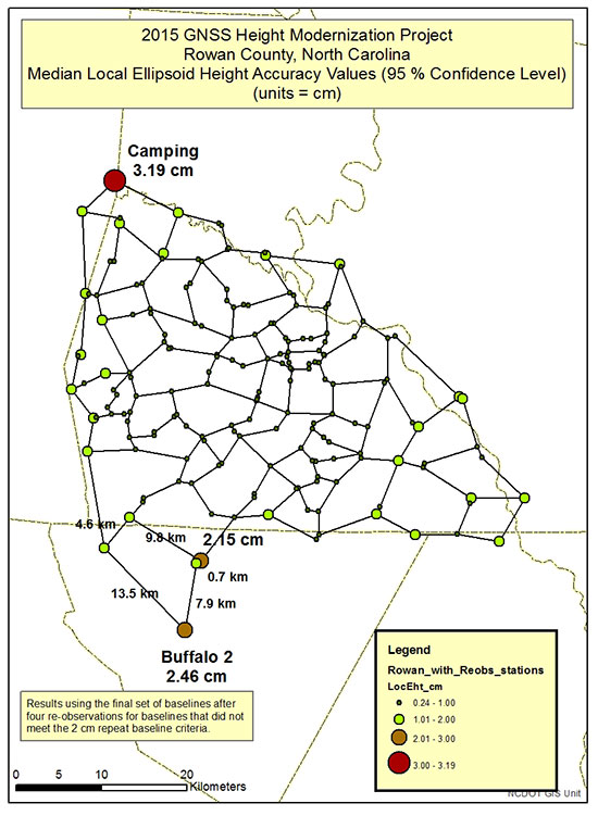
It is important to understand the quality of the adjusted ellipsoid heights. When analyzing the project’s ellipsoid heights, the user should compute the local ellipsoid height accuracy values. Part 2 discussed NAD 83 (2011) network and local accuracies. NGS’ adjustment program has an option of computing network and local accuracy values.
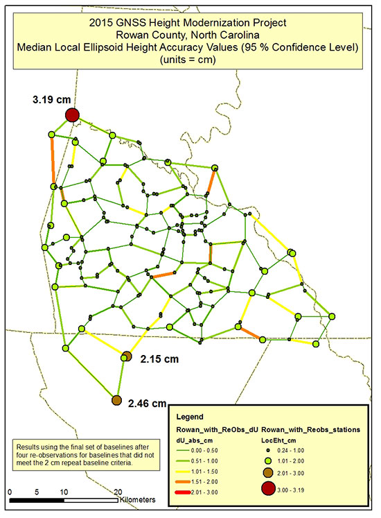
Figures 7 and 8 are plots of NCGS Rowan County GNSS Height Modernization median local ellipsoid height accuracy values. Stations that have local ellipsoid height accuracy values greater than 2 cm should be investigated. Figure 7 highlights the two largest median local ellipsoid height values [Camping (3.19 cm) and Buffalo 2 (2.46 cm)]. The observations and residuals of the baselines in the area should be closely analyzed.
Figure 8 is a plot of the local ellipsoid height accuracy value with the absolute dU residual values. If the user follows all of the NGS 58 guidelines, then all baseline residuals should be small (less than 2 cm). In this project, the largest “dU” residual is 1.86 cm. Saying that, the network design could be modified to try to improve a station’s median local ellipsoid height accuracy value.
For example, station Buffalo 2 has a median local ellipsoid height accuracy value of 2.46 cm (see Figure 7). It’s only involved in one loop, and it’s relatively large. The loop has five baselines consisting of lengths of 13.5 km, 9.8 km, 7.9 km, 4.6 km and 0.7 km. Two of the baselines lengths are greater than the guideline’s average baseline recommendation of 7 km, but all repeat baselines meet the 2 cm guidelines, and all residuals are “reasonable.” Adding another baseline between two different stations to create two smaller loops from the one larger loop would decrease the size of the loop and increase the redundancy in the network.
In this particular case, station Buffalo 2 has a published NAD 83 (2011) ellipsoid height, and the difference between the adjusted height and the published height is only 1.1 cm (Figure 5), indicating the new survey is consistent with the old survey. Station Camping also has a published NAD 83 (2011) ellipsoid height, and the difference between the adjusted ellipsoid height and published height is -1.9 cm (Figure 5). Once again, this indicates that the Rowan County GNSS survey is consistent with the previous survey.
This column focused on describing procedures for analyzing a project’s GNSS-derived ellipsoid heights. As previously stated, it important to ensure that your GNSS-derived ellipsoid heights meet the desired accuracy of the project before using the survey data to estimate GNSS-derived orthometric heights.
Figure 7. Plot of NCGS Rowan County Height Modernization project’s median local ellipsoid height accuracy values.Figure 8. Plot of NCGS Rowan County Height Modernization project’s median local ellipsoid height accuracy values and absolute dU residuals.
So far, this series has addressed the following topics:
basic concepts of GNSS-derived heights
NGS’ guidelines for establishing GNSS-derived ellipsoid heights (NGS 58)
differences between hybrid and scientific geoid models, and
procedures and tools for detecting GNSS-derived ellipsoid height data outliers.
These four columns were meant to provide the reader with basic concepts and procedures for estimating GNSS-derived ellipsoid heights.
My next column, which will appear in the February 2016 Survey Scene newsletter, will discuss procedures for estimating GNSS-derived orthometric heights. Determining valid NAVD 88 published heights is very important when using GNSS data and geoid models to estimate GNSS-derived orthometric heights. NGS has documented these procedures in NOAA Technical Memorandum NOS NGS-59. The NGS 59 guidelines are separated into three basic rules, four control requirements and five procedures that need to be adhered to for computing accurate NAVD 88 GNSS-derived orthometric heights. The next column will address the NGS 59 guidelines.
Topcon Positioning Group is collaborating with DAQRI, an augmented reality company, on wearable technology designed to change the way construction and survey professionals interface with the job site.
DAQRI is the creator of the DAQRI Smart Helmet, an industrial-grade wearable that seamlessly connects humans to their work environments by providing information about the world around them.
Topcon and DAQRI will work together to create a solution designed to make workers on the job safer and more productive through the use of augmented reality technologies. They plan to do this by integrating DAQRI’s hardware and software solutions with Topcon positioning solutions.
The DAQRI Smart Helmet was designed for the industrial workplace. It includes an advanced sensor package, an intuitive user interface that requires zero calibration, and a battery that lasts a full shift.
Powered by 4D Studio, DAQRI’s software platform for positioning, the partnership will allow construction workers to view information from their projects in the real-world work environment to make their workflows safer and more efficient.
The collaboration is designed to bring wearable technology to a wider AEC (architecture, engineering and construction) user base, empowering the wearer with a hands-free tool that can be used on the job, Topcon said in a news release.
“DAQRI is a leader in providing solutions in outdoor environments, which will meld well with our positioning and software innovations,” said Jason Hallett, Topcon vice president of product management. “It’s the first step in utilizing our mutual synergies to develop rugged, heads-up display technology for our marketplace.”
“We are committed to developing innovative solutions that power the future of work and Topcon is at the forefront of the industry with some of the most innovative products that are being used by millions of workers across a variety of environments,” said Matt Kammerait, vice president of product, DAQRI. “This makes them the perfect partner to integrate the Smart Helmet into existing workflows. We look forward to seeing how our partnership re-defines the nature of ‘work,’ by setting a new standard for wearables in the AEC space.”
When a GNSS RTK base station is started by assuming an autonomous position, it is necessary and good practice to later adjust and correct the coordinates with a solution referenced from known coordinates. JAVAD’s field software for the TRIUMPH-LS, J-Field, has the ability to adjust the RTK base station coordinates and RTK points surveyed using corrections from that base station.
Three methods can be used to accomplish this.
Manually Entering New Base Station Coordinates
Base station coordinates can be updated manually by entering new coordinates for the base station. These new coordinates can obtained through post-processing the base station data with OPUS or JAVAD’s DPOS web interface. Follow these steps to apply the corrected coordinate to the base station and adjust all the points from this base station through J-Field:
Select an RTK or base station point in the Points screen.
Tap on the blue screen displayed on the right side of this screen to view the Base Rover Statistics screen.
Tap the Base button and you will be prompted to enter the corrected coordinates for the base station.
Enter the new coordinates and tap OK.
J-Field will then search for all the points contained in the current project with the same original matching base station coordinates and apply offsets to adjust all these coordinates into the known coordinate system. The adjusted coordinates along with the original base station and surveyed origin coordinates will still remain stored in the database for documentation purposes and so that adjustments can be undone or modified if necessary.
Base Rover Statistics screen.
DPOS
When a Javad base station is started with J-Field using Base/Rover Setup, the raw GNSS data is automatically saved in the base station receiver. When the base station is then stopped with Base/Rover Setup, the data is downloaded into J-Field so that it will be available for post processing DPOS. To post-process the data, open the DPOS tool found in the CoGo menu and select the base file you wish to process. With the TRIUMPH-LS connected to the Internet, tap the DPOS button to upload the file to DPOS. This automated process will then update the base station and RTK surveyed points using the same algorithm described above.
Shift Mode
The newest feature of J-Field, Shift Mode, allows real-time corrections to be applied to receive base station corrections. A base station can be started with an autonomous position and then corrected by surveying a point with known coordinates. The known point could be a point previously surveyed with a base station setup in a different location. This feature is useful for several scenarios:
You need to move or “leapfrog” your base station to extend the radio range into a new area.
Your original base station point has been lost.
You wish to save time by starting the base station with it mounted to the top of your vehicle. Setting the base station and radio up on the top of vehicle by mounting it a roof rack or using a magnet mount saves time by eliminating the need to set up tripods and can help protect the base station from disturbances or theft in undesirable locations. For the best performance, the base station should be mounted in a level position so that phase center variations and antenna offsets are correctly applied. If you are parked on a sloped surface, it may be necessary to use a tribrach to level the receiver on the top of your car.
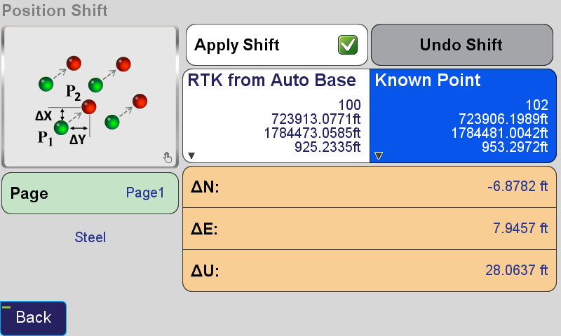
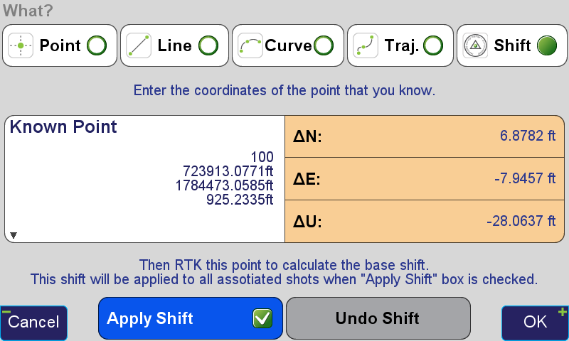
The Real-time Position Shift function can be accessed from the Setup menu under Advanced. In this screen, select a point you have collected RTK coordinates from with an autonomous base station, and then the known coordinates of this point. Check the Apply Shift and the shift will be applied to all the RTK surveyed points found in the current project collected from this base station. This shift will continue to be applied to all the points surveyed from this base station.
Position Shift screen.
Real-time Position Shift can also be accessed from the Collect Action screen by clicking the button below the Start button and changing the collection mode to Shift. In this mode, select the Known Point and then press Start from the action screen so that the offset can be calculated. After it has been calculated, you can apply the shift.
Position Shift screen from the Collect Action screen.The Collect Action screen in shift collection mode displaying the Accept/Reject Prompt for the shift.
One of the newest developments in J-Field, JAVAD GNSS’s onboard data collection software, is the Reverse-Shift. This feature will allow you to mount a base on a magnetic mount to the top of your vehicle, instead of putting your base on a tripod.
This is a good idea for several reasons. First, you won’t have to worry about your tripod sinking in hot asphalt. Second, you will not have to worry about your tripod fading on frozen ground that begins to thaw.
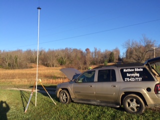
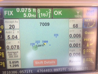
Figure 1. My TRIUMPH 2 base mounted above my driver-side door on the roof, with my 35-watt radio and antenna just to the left.
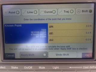
The way Reverse-Shift works is by starting your base on an autonomous position. Once your base has started transmitting, you can then go into your collect screen and change the point tab to shift. You then have the ability to select a known point (a previously surveyed or calculated point). After you have selected this known point, you can go and survey that known point.
Figure 2. The shift screen showing the known point (previously surveyed point).
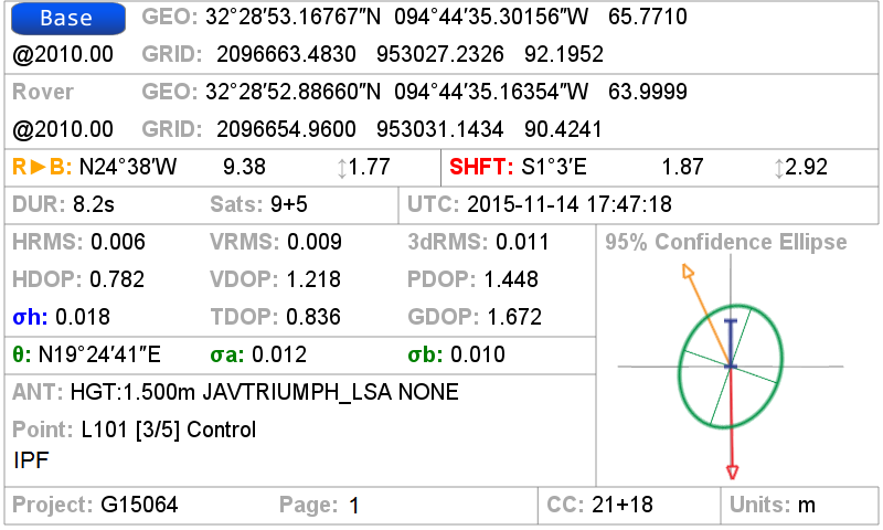
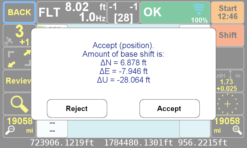
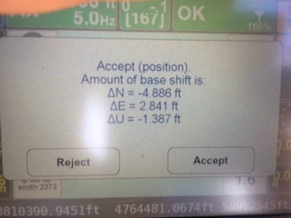
When you hit OK as shown in Figure 2, this will take you back to the collect screen, and then it will allow you to survey that point. It will give you an warning screen that states, “You are in Base Shift Calculation Mode, Do you wish to continue?” You will then be able to collect a surveyed point on the previously surveyed or calculated point. It will then give you the position shift information.
Figure 3. The adjustment parameters for the base.
Hit Accept, and this will adjust your base position by the stated difference, allowing you to continue to work on the known coordinate system without setting your base on a known point.
Figure 4. Staking back out to the (known point) after the Reverse-Shift has been completed. Notice the DTT (Distance To Target) is 0.006. degrees.
At the end of the day, when you go back to your base, hit “Stop Base”. This will download the static data out of your base into your TRIUMPH-LS rover.
The next morning when the CORS data has been uploaded, you can then post-process your base data using DPOS (JAVAD’s Data Processing Online Service). With DPOS you can then adjust your base to the TRUE state plane coordinate of where your base was actually sitting. It will also adjust all surveyed points that were collected from that base position.
For more information on JAVAD’s J-Field software, the TRIUMPH-LS or other JAVAD GNSS solutions, please feel free to visit www.javad.com, email [email protected], or call 1-888-550-5301 or 1-408-770-1770.
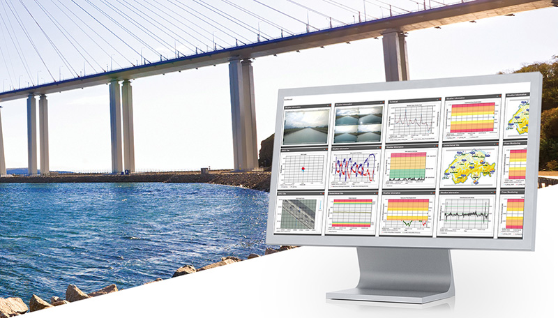
Leica Geosystems has introduced two new additions to its Leica GeoMo deformation monitoring solution: Leica GeoMoS AnyData and GeoMoS API.
Users of the system can now create comprehensible visualizations and customizable reports, which enables powerful sensor data fusion for applications, such as air or water quality monitoring and construction or building management.
With GeoMoS AnyData and GeoMoS API, multiple open interface standards are accessible to provide even more information to projects than just classic geodetic monitoring applications, according to a news release from Leica. The open solution offers flexibility; it is capable of automatically acquiring, processing and distributing intelligent information locally or via the Internet in real time.
Leica GeoMoS integrates, processes and distributes all project data within one software program.
“Monitoring professionals are confronted daily with vast amounts of data collected and provided by a variety of sensors,” said Michael Rutschmann, senior product manager of Structural Monitoring at Leica Geosystems, in the news release. “With these additions to Leica GeoMoS, all information is now easily accessible via web-based visualisation. This is absolutely the most efficient way to convert raw data streams into intelligent information for any user.”
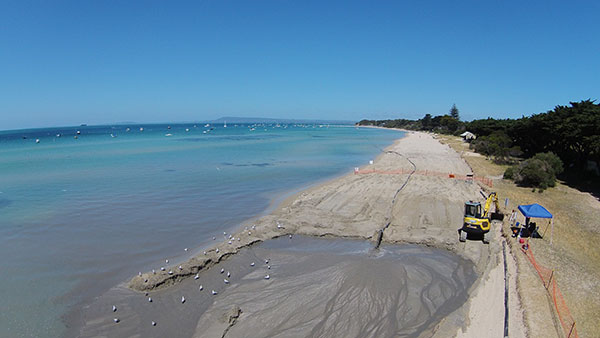
Shifting sands in Australia’s Port Phillip Bay left a popular beach without enough sand this past holiday season. As summer approached, the Mornington Peninsula Shire and Australian Department of Environment and Primary Industries (DEPI) decided to replenish Sorrento beach by dredging a nearby sandbank.
DEPI awarded the contract to Sandpiper Dredging because of its history of minimizing environmental impact. Sandpiper has a decade of dredging experience and builds its own precision dredgers in Tweed Heads, New South Wales.
Erosion of Sorrento Beach required high-tech repairs. (Photo: Trimble)
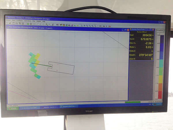
The contract specified the dredge ground extent and the minimum Australian Height Datum (AHD) height Sandpiper could dredge. To obtain precise 3D positions from the GPS receiver, GPS corrections were streamed in via cellular Internet from the Victorian government’s Continually Operating Reference System (CORS). Position and heading from the SPS461 receiver were interfaced into construction software to display dredge position. The inclinometer mounted on the dredge frame also interfaced with the software and allowed the AHD height of the cutter head to be displayed.
The dredge position displayed in the software allowed operators to stay within the dredge grounds and ensure no over-dredging occurred. The software was the central hub in the wheelhouse displaying and logging dredge positions and the AHD height of the dredge head.
Machine-control positioning enabled Sandpiper to precisely place in 3D the cutter suction head on the dredge frame in real time. (Photo: Trimble)
The software also allowed the dredge operator to focus on controlling the dredge rather than trying to determine where to dredge. Using GPS and AUSGeoid09 removed the need for considering tide data because the software displayed the AHD height. The logged data could be delivered to the client as an as-built drawing.
The beach was replenished within budget and on time for the holiday season, and the community is now enjoying the restored beach.
Hydrographic Tech
To achieve the job specifications and efficient operation of their dredge, Sandpiper needed hydrographic survey technology on board. SITECH Construction Systems, a Trimble distributor, provided the company with:
Trimble SPS461 GPS heading and positioning receiver
Inclinometer to measure the angle of the cutter head frame
Trimble HYDROpro dredge software to display and log seabed levels. The software can be configured for a wide range of dredgers.
“After speaking about the challenges we had been facing, SITECH came back with the solution of the Trimble HYDROpro system, which meant we could dredge in exactly the right place and maintain coverage, all the while protecting the environment of the beach,” said Daniel Fristch, owner of Sandpiper.
HYDROPro at work on the Sorrento Beach project. (Photo Trimble)
Handheld Group’s new Algiz RT7 tablet is designed for rugged use by mobile workers.
Handheld Group, a manufacturer of rugged mobile computers, today announced the launch of its new Android tablet, the Algiz RT7. The Algiz RT7 is a powerful, lightweight and ergonomic 7-inch tablet designed for reliable performance in demanding environments.
The Algiz RT7, which runs Android 5.1.1 (Lollipop), provides a range of features for mobile workforces, Handheld said. It’s fully rugged, meeting stringent MIL-STD-810G U.S. military standards for protection against drops, vibrations and extreme temperatures, and its IP65 rating means that it’s waterproof as well as fully sealed against sand and dust. Weighing just 650 grams, the Algiz RT7 is designed for mobility.
The Algiz RT7 comes with a built-in accelerometer, gyroscope and e-compass and a stand-alone u-blox EA-7M GPS receiver for navigation, along with built-in Qualcomm IZat location services.
A Qualcomm MSM8916 (Snapdragon) chipset and 1.2 GHz quad-core processor power the tablet, giving it processing speed, ultra-fast connectivity and long battery life. It comes standard with LTE data and voice capabilities as well as 802.11 b/g/n WLAN, BT Class 1 and Class 2, and NFC functionality. It also has dual cameras (8-megapixel rear-facing and 2-megapixel front-facing), as well as dual SIM-card slots.
Designed for the mobile worker, the Algiz RT7 sports a high-brightness 7-inch outdoor-viewable capacitive display that can handle true outdoor challenges. Battery performance is key for any mobile application, and the Algiz RT7 comes with a long-life 3.7V 6000mAh lithium-ion battery. Four programmable buttons allow users to launch and use applications in the field. To enhance data capture, users can choose an optional 2D imager or RFID plus 2D imager.
“Our new Algiz RT7 offers enterprises an exceptional value and is a highly requested product from both our end users and our extensive partner network,” said Jerker Hellström, Handheld Group CEO. “This ultra-rugged tablet delivers best-in-class performance to assist fieldworkers in their daily tasks. The Algiz RT7 is built for tough environments and delivers a streamlined Android experience with power and features appropriate for market demands.”
The Algiz RT7 can be ordered immediately. Shipping will start in December, with volume deliveries starting January 2016.
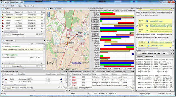
Carlson SurveyGNSS, Carlson Software’s data post-processing software, is now available in a 2016 version.
Designed for surveyors and positioning professionals, Carlson SurveyGNSS post-processing software achieves high-accuracy results for computing quality vectors and resultant positions. SurveyGNSS works with Carlson SurvCE and SurvPC data collection software, and with Carlson’s office design software.
New features include a second-generation post-processing engine, which now accepts data in enhanced RINEX 3.x formats. Users will also determine candidate vectors for simultaneous calculation. Previously, vectors were calculated individually.
Other processes have been sped up or enhanced. With “detached processing,” users will be able to start another task while SurveyGNSS is still working on a computation.
New constellation and more reference networks are another enhancement. Observations from the Chinese BeiDou and European Union Galileo join GPS and GLONASS, with future constellations in the works.
For supported “Active” (Online) Reference Networks, the International GNSS Service (IGS) and the governments of Australia, Brazil, Canada, Germany, Spain, European Union, France, Great Britain, Mexico and the Netherlands join the supported networks in addition to the U.S. CORS system.
In the temperate rainforest of the Los Lagos region of Southern Chile, where rainfall annually exceeds 1,500 millimeters and two-thirds of the days are rainy, the dense forest canopy poses a huge challenge for GNSS receivers.
Motivazion, a survey firm based in Puerto Montt, just below the rainforests, makes its living surveying in the rugged terrain under the densely canopied forest. Motivazion works primarily for hydropower development companies, surveying contours, cross sections and longitudinal profiles, as well as staking out proposed facilities. To ensure it was using the best GNSS receivers for the conditions, Motivazion conducted field tests of several sets of equipment this summer.
Motivazion owner Jorge Mesias said he typically uses a combination of total stations and GNSS receivers for his work. “If understory performance could be improved, efficiency would increase dramatically and reduce the need for using the more time-consuming total station,” Mesias said.
A light rain fell at all times during the two-day test. The test routine consisted of surveying a total of 21 points in two days. Results were compared to points established by a total station.
Base stations were set up in a small area cleared for the purpose, and the rovers moved from point to point under the canopy. Spectra Precision’s SP80 achieved fixed solutions in less than three minutes 95 percent of the time.
“The SP80 achieved remarkable results,” concluded Mesias. Geocom S.A., Spectra Precision’s dealer in Chile, provided the SP80 and technical support.
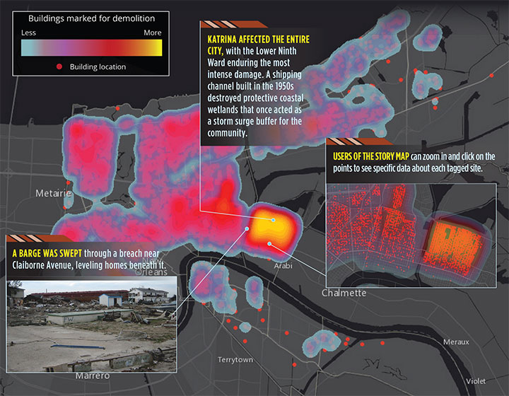
In August 2005, Hurricane Katrina struck the city of New Orleans, causing devastating damage and loss of life. A new Esri story map, “Katrina +10: A Decade of Change in New Orleans,” analyzes the damage from the storm.
“The story map is a new Esri medium for sharing not only data, photos, videos, sounds and maps, but for telling a specific and compelling story by way of that content,” wrote Esri Chief Scientist Dawn Wright in a blog. “This is all done with sophisticated cartographic functionality that does not require advanced training in cartography or GIS.” According to Wright, story maps are applications built from web maps, which in turn are built from web-accessible data.
The below map shows the physical damage in terms of buildings marked for demolition. In all, 10,317 buildings were tagged for demolition by the city of New Orleans. Following Hurricane Katrina, all properties within the city were reviewed for damage under Section 106 of the National Historic Preservation Act.
The heat map shows the density of houses deemed eligible for federally funded demolition through the Federal Emergency Management Agency (FEMA). Although not all properties on this map were demolished, the points illustrate Katrina’s extensive and pervasive physical toll on the city of New Orleans.