In following up on my example of a simple GIS app for entering and displaying lat/lon coordinates from a spreadsheet (or text file), the discussion went from cloud to client and then back to cloud. The reason may surprise you. Recall that I was looking for the best solution for a reader who was looking for a simple GIS app to display gobs lat/lon coordinates.
My first inclination was to use an online app (cloud) such as arcgis.com or Google Earth in order to stay away from the users needing to install and maintain software on their local desktop computers. No go. The functionality just wasn’t there. All along, my backup plan was to use a client app like ArcGIS Explorer. Well, after messing around a little and consulting with an online discussion group, that’s the route I went. I wrote about it last week.
Subsequently, a GIS manager from a public department (state level), wrote about his experience with client-based apps and his challenges with IT outsourcing. It really make one reconsider the cost effectiveness and efficiency of IT outsourcing. His perspective makes interesting reading:
We didn’t go the ArcGIS Explorer route primarily because of the current war (GIS vs. IT) which scientific computing is losing badly at this point in time. Our State and many others are neck deep in smelly muck created by business computing’s IT consolidation and outsourcing. I just got back from a meeting where I heard another round of horror stories from VA.
For more than five years, our WAN-based users at regional offices throughout the state have ran GIS via Citrix with customized ArcGIS desktop apps written entirely in-house by our staff in VB and .Net. We elected that strategy because at that time it was really the only serious option to allow access to the large amounts of data we had in our geospatial archive here at our headquarters. It was also attractive because back then we controlled our infrastructure and our LAN and were highly influential in WAN decisions because we had a very advanced computing environment here.
Then came IT consolidation and the predictable downgrading of advanced Agency’s capacity so we’d be able to open really big word processing documents on our desktops. By that, I mean scientific computing like GIS, Remote Sensing, etc. apps were not considered seriously in that process even though we need to operate much closer to DoD or NGA-like computing capacity compared to the average accountant. After multiple attempts to modernize our Citrix and SAN, resources were turned down and we decided we’d better switch to a new approach.
Because we’re charged serious bucks every time we put in a service call to have ArcGIS Explorer installed on an existing or new PC, we elected to go as thin client as possible. Everyone has a browser and we don’t have to pay to have that installed. We initially developed some betas using ESRI’s JavaScript solution but browser differences (both different versions of the same browser and Microsoft vs. Firefox on individual PCs just inside our unit) caused many applications development problems so we abandoned development with that API.
That’s when we elected to do a very serious Flex vs. SilverLight comparison and the rest is history. The new beta has a rainfall widget we’re particularly proud of. It grew out of our active mining program staff having to respond to horrific flash flooding typical in spring and summer in our state. This new app will allow staff to go to the permitted sites to check stability of sediment control structures where the most rainfall (… based on Nexrad) was projected to have fallen for the first time this spring.
In April this year we’ll find out if our jobs are going to be outsourced or whether our state will modernize internally. The refusal to allow Citrix and SAN improvements is a harbinger of the way that will go I believe. We have been presented with 4 SAGs in the last decade. I wonder what the total count will after the first decade of outsourcing?
Many potential problems exist for geospatial programs because of IT consolidation and the more recent potential of outsourcing GIS. IT consol first. My unit does a great many very large (… and long) computing jobs. We routiinely move data from one projection or datum to another. When you deal with thousands of raster tiles, a reprojection project can take weeks to accomplish successfully. We also do spatial analysis projects that take even longer. We recently used Landsat scenes and higher resolution commercial satellite data plus aerials from multiple dates to do change analysis. That job took more than a month on beastly PCs we’ve built up specifically for these very tough jobs.
[[Our]] ICI is an old DoD concept I pulled back into use. We built these platforms after about a year of total frustration having our big jobs crashed from IT pushes of OS upgrades happening in the middle of producing badly needed new deliverables, network disconnects dropping out our license checkout connectivity to a remote license manager on the WAN, etc. I’ve already mentioned the failure to consider geospatial in upgrading infrastructure and improving bandwidth.
Even keeping your servers local can be a big battle in the war. We have an older county size LiDAR dataset (pre-.las) processed and delivered as a point cloud. We have new LiDAR from the same county and we’re trying to do a comparison of the two datasets. Depending on what USGS quadrangles are selected it typically takes 30 to 40 minutes to load up four 1:24K quad size tiles of the older point cloud data via our LAN at fast Ethernet speed. Move that to a WAN situation and we need to start it loading in the evening so it’s ready by the following morning (but that won’t work because of the auto-shutdown software on all the desktops that executes every evening a 7PM). And then there’s the joke about the virus checking software pushed out to every desktop, configured all the same for everybody and auto executed and the twenty-one staff that mapped over five terrabytes of GIS datasets on the SAN and their very fast new computers (sarcasm) being brought to the approximate speed of molasses running up hill because the virus checking code never stopped trying to check all five TBs on each of the twenty-one PCs. It wasn’t much of a joke when the whole Agency’s networking speed dropped to a crawl! Need I say more about one-size-fits-all IT mentality shooting off their own feet!
Negative aspects of outsourcing geospatial jobs are obvious. No contractor is going to know the individual program requirements like in-house staff and that’s a challenge even for us. Good example … the rainfall widget on the new beta app I pointed you to wasn’t requested by our mining folks until we approached them with the idea that we might be able to do something like that. Would there have been that kind of insights by a big corporate consulting firm like IBM or HP? I think not.
On the good side of IT consolidation, if geospatial folks are pulled together into a core group I think that gives folks the chance to work on a broader spectrum of tasks not limited by the bounds of what one state government Agency desires, but rather the state as a whole. That could be a good thing. Also, it gives Agencies with a GIS effort, consisting of one or two folks, access to experts they’d not be able to otherwise tap into (GIS DBAs, geospatial applications development gurus, etc.) and that definitely would be a very good thing. Of course that hasn’t happened here. On the good side, with outsourcing GIS jobs, I’m clueless as to how that could ever benefit anyone except the recipient of the contract. The horrible stories from colleagues give me night terrors. PC refresh cycles of 5 years, horrendously expensive SAN storage rates, etc. You name it, &
nbsp;the customer is hosed by it.
There really is a business vs. scientific computing all-out war going on all around us and as I said initially, too many scientific computing types have their heads down doing the exciting stuff while the fight rages on, without them even knowing about it. If you can wake them up to the reality that business computing “experts” may very well be building a scientific computingless future in which they’ll have no place (or job), it would be greatly appreciated.
I’ll be writing more about this. It’s a serious issue and it’s not going away, especially with the geospatial industry continuing to put up strong growth numbers.
I’m preparing for some conference presentations I’ll be giving in a couple of weeks. One of the subjects I’m covering is spatial data transformation, or traditionally known as ETL (Extract/Transform/Load) tools. I’ve written many times before that in the geospatial industry, data is the fuel. We, as users, have access to some amazingly powerful GIS software tools.
Clearly, the geospatial enabler is data. Without it, it’s like having a fishing pole without a pond; a tool without a purpose.
If you look at emerging geospatial technologies, where’s the data coming from? Yes, crowd-sourcing, GPS/GNSS, and imagery are, and will continue to be, volume sources of geospatial data.
From an infrastructure perspective (civil engineering), 3D laser scanning is a particularly interesting source of high-volume geospatial data. Ground-based and airborne 3D scanners create insanely huge volumes of data. Although an emerging technology, these scanners (LiDAR technology) have been around for many years.
I recall using this technology on projects 8 or 9 years ago to scan accident scenes and infrastructure such as bridges. The scanning time was amazingly efficient. In some cases, the scanning data collection sessions were done in a couple of hours. During that period, literally millions of data points were collected. For the first time, the ratio between labor expended on data collection and labor expended on data processing was extremely skewed towards data processing, and that was the headache.
While scanning time was very short, data processing time to produce a deliverable was brutal, literally taking weeks. Granted, that was 8 or 9 years ago. Advanced software tools have made data processing more efficient today, but dealing with huge volumes of data is still a challenge. Some people say that scanning may eventually replace traditional surveying equipment that shoot and record one coordinate at a time. A land surveyor, on a really strong day, may be able to shoot and record upwards of a 1,000 coordinates. With a scanner, that same person could shoot and record millions of points in a day.
Data, Data, Data
Ground-based and airborne LiDAR technology are clearly on the uprise. Last year, while most conferences were struggling to maintain the 2009 levels, even failing, the SPAR 2010 3D imaging conference was up 23%, according to their reports. The International LiDAR Mapping Forum conference also reported record attendance figures. Although the conferences are still in niche-mode (less than 1,000 attendees), the growth is steady.
If you step back a bit and look at the big picture, the game is in data processing. Yes, equipment manufacturers will crank better and cheaper scanners, but turning those 3D point clouds into useful products is where the action is.
You can see this with SAFE Software’s recently announced FME 2011 product. While historically focused on GIS and CAD interoperability, SAFE obviously sees the upside in the point cloud business as a major part of FME 2011 is focused on dealing with the massive amounts of data created from 3D laser scanning.
Keeping it Simple
Changing gears…
With all this geospatial technology advancing faster than a rabbit on a motorcycle, it’s hard to slow down and look at the simple uses of GIS that still offer a lot of value. As much as most of us are pushing hard to implement more and more spatial data technology, it’s just as important that we introduce people to GIS, even a very simple version of it.
This week, a reader asked me about the best way to display a map from a bunch of lat/lon coordinates (little or no attributes) in a spreadsheet. No complex attribute tables, no strange map projection, just a spreadsheet of lat/lon coordinates.
This challenge gave me reason to revisit Esri’s freely available ArcExplorer software. It wasn’t my first choice, but it’s where I‘ll likely end up. I haven’t touched ArcExplorer (I know that’s not the name of the current software, read on) for quite some time (as in a couple of years or more). I use ArcGIS, AutoCAD and a half-dozen other spatial data software tools.
When presented with the challenge, my first inclination was to push her towards arcgis.com in order to steer her away from having to download, install and maintain desktop software. No go. After a quick post to a support group, I’m told there’s not an easy way to add this data to an arcgis.com map. My other thought was Google Earth. Naah.
I subscribed to Google Earth Pro for a year and it really is sort of cheesy, to me. Maybe it’s because my view is distorted from my experience with GIS software in the past, but it seems to me that Google Earth is still primarily eye-candy, and what I really wanted was an easy-to-use, light-weight GIS. However, I do hope that they continue pushing that technology forward.
All along, I thinking my ultimate back-up plan would be to recommend ArcExplorer. I went to download it and remembered it’s now upgraded to ArcGIS Explorer. I remember reading and posting that news awhile back, but hadn’t taken the time to download and preview it. It’s a much different animal than ArcExplorer, and I like what I see so far. I haven’t tried to import any data yet, but from the menu selection, I can see it will accept the simple ones such as shapefiles, raster imagery, ASCII, and GPS exchange files. Most simple data sets can be converted to one of these formats using freely available software tools.
ArcGIS Explorer Opening Screen
This will be an interesting experiment, and one I will update you on, likely next week, as I try it with a sample data set from the reader.
I really like the opportunity to introduce someone to GIS, even at just a simple level because I believe will open their eyes to other possibilities in the future. It empowers them to think more GIS-centric.
LizardTech announced the integration of its MrSID Generation 4 (MG4) SDK into Global Mapper version 11.01. Until recently, Global Mapper’s customers were not able to load point cloud datasets that were compressed to MrSID Generation 4 using LiDAR Compressor into Global Mapper. However, with the addition of support for MG4 in Global Mapper version 11.01 users can load point cloud datasets compressed to MrSID Generation 4 for use in volumetric analysis, contour generation, and visualization.
“Adding MG4 integration to the latest version of Global Mapper is just another step to ensure that our customers have as many mapping tools possible at their fingertips,” said Mike Childs, Global Mapper Software LLC. “Based on user feedback, we believe this integration with LizardTech will bring added value to our customers.”
“LizardTech’s goal is to give customers tools for using their point cloud data compressed with LiDAR Compressor in the applications they use every day,” said Jon Skiffington, LizardTech’s director of marketing. “Many of our customers use Global Mapper, but were not able to use it with MrSID files created in LiDAR Compressor. Now our customers can easily load point cloud datasets compressed to MrSID Generation 4
into Global Mapper.”
The place to be if your job is intelligence and why what is where.
By Art Kalinski
When I was in graduate school at the University of North Carolina at Charlotte, Dr. Jerry Ingalls shared a succinct description of the “new” geography. He stated that old geography was merely the study of where everything was. However, new geography, with its spatial analysis tools, had significantly expanded the field of the study to “why what is where” and knowing why we can start predicting new “wheres” based on known facts. That, of course, is where geospatial intelligence is today, and some of those tools and techniques identified the location of Iranian nuclear facilities long before they became public knowledge.
Learning about the latest tools and techniques is the primary reason for conferences, and there is agreement in the geospatial community that GEOINT is the place to be. Organized by the United States Geospatial Intelligence Foundation (USGIF), attendance at the San Antonio conference was the highest it has ever been, according to USGIF President Keith Masback. Even with a weak economy, the over-arching opinion of all attendees was that the intelligence business will continue to grow regardless of world politics. By its nature, this conference really had many more “chiefs” than “Indians,” and many exhibitors spared no expense at the conference, knowing that they were reaching key decision makers.
USGIF, a nonprofit educational organization created by the geospatial intelligence community, is the organizing force behind the conferences. There is heavy participation by the National Geospatial-Intelligence Agency (NGA) and other intelligence agencies, so the conference attracts top executives in the geospatial industry. The speaker and attendee list reads like a who’s who of the geospatial and intelligence fields.
General Clapper, the Under Secretary of Defense for Intelligence, was a keynote speaker. He stated his belief that regardless of geopolitical decisions, he sees no decrease in the need for intelligence in Afghanistan and many other locations around the world. He further addressed the need for much faster turn-around of actionable intelligence and cited the joint efforts between the SIGINT (Signals Intelligence) and GEOINT (Geospatial Intelligence) communities.
General Clapper discussed some of the work of the ISR (Intelligence, Surveillance, Reconnaissance) Task Force, which is seeking new technology and the Holy Grail of intelligence, automated target identification in complex environments. He also spoke about the benefits of commercial imagery sources and its use in an impressive NATO Fusion Center he toured.
The second keynote speaker was Representative C. A. Ruppersberger, D-MD, chairman of the House Technical/Tactical Intelligence Subcommittee. The congressman addressed his concern that the U.S. is in danger of losing its preeminence in space because regulations are hampering development. He specifically addressed a need to overhaul International Trade in Arms Regulations (ITAR) that are hurting the U.S. commercial satellite industry. He also stated the need for additional research and development funding like the ones that built the U.S. space program and a greater emphasis on technical education. A troubling statistic he cited is that China has 440,000 engineers compared to the USA’s 65,000.
Vice Admiral Murret, head of NGA, then spoke of his agency’s support not only for the military but humanitarian assistance in natural disasters such as flooding and earthquakes. He talked about the new NGA facility at Fort Belvoir and about how one third of his agency now works in St. Louis.
In the exhibit hall close to 200 exhibitors demonstrated their latest efforts. Some highlights include:
Cogent3D and Lockheed Martin demonstrated the release of GeoSketch, a plug-in for Google Sketch Up. GeoSketch permits military users to build 3D models using the easy to use Google Sketch Up software. The tool permits users to import military UAV video imagery, oblique imagery, and other photo sources to rapidly build 3D models even if geo-referencing data or camera models are missing. The models can then be exported in common formats such as Google, Multipatch, or OpenFlight.
Digital Globe announced the successful launch of its newest high-resolution satellite, WorldView 2. Imagery from the new satellite will be available in a few months, doubling Digital Globe’s image-collection capability, including multi-spectral imagery.
LEXISNEXIS news open source highlighted the tremendous wealth of data that it makes available to intelligence analysts. Appistry and NJVC had extensive information on cloud computing and their ability to deliver mission-critical data, including legacy data, to users around the world.
Pictometry and Lockheed Martin announced their alliance and creation of a new service, Intelligence on Demand (IOD). IOD promises to be a game changer. (See October’s column for details.)
Every conference I attend there is always a new technology that really catches my eye. Ball Aerospace was demonstrating such a technology, Flash LIDAR. Flash LIDAR has been a laboratory curiosity for a while but Ball Aerospace has made it a functional tool. Most current LIDAR collections use a laser to scan the ground with the return being sampled resulting in a collection of points on the ground that provide elevation data from which a DEM or contour lines are created. Although this is a rapid process it is sequential and not instantaneous. The resulting data can be very coarse or fine depending on the sampling interval.
Flash LIDAR is what the name implies; an entire area is imaged in one nano-second flash. The laser is diffused over an area and flashed once. The resultant image is a broad but dense sample taken at the same instant rather than through a scanning process. Since the image is taken from the same point at the same instant, the data can be used to create accurate 3D models. Those models can then be draped with photographic images or even video frames. The process is so fast that 3D models can be created almost in real time.
The below images are a practical demonstration of the Ball Aerospace process using Flash LIDAR combined with a live video camera. As each frame of the video image is taken, a simultaneous Flash LIDAR image is also taken from the co-located LIDAR unit. The photo shows the live video and point representations of the Flash LIDAR 3D surface and the resultant 3D image draped on the moving 3D model.
It’s hard to tell from these still 2D photos but seeing this system in operation was impressive since the Flash LIDAR and resulting 3D models were continuous and perfectly registered. The only limitation of this demonstration was that human flesh is not a good “Reflective Surface.” Note that in the photo the Ball representative was very animated. This stop-action screen-capture shows him as he jumped up. In all cases the Flash LIDAR kept up with the dynamic movements.
Point cloud.Point cloud.Point cloud.Wire-frame image.
This was an impressive conference that suffered from too much in too short a time. Two tools that were very helpful was a daily newspaper, the Show Daily, that recapped the previous day along with the current day’s schedule. It was published, printed, and placed under our doors as we slept. The other useful tool was a daily video show with key presentations and interviews for those that were unable to be in two places at the same time. It was available at several break locations and on our in-room TVs. This has been done at other conferences but not as well as the execution of USGIF.
The usage of three dimensional data in the geospatial industry is in its infancy. It makes sense to me. Sometimes, it’s hard enough for folks to obtain and maintain accurate two dimensional data, not to mention elevation! However, as geospatial technology continues to evolve, the availability of 3D geospatial data will evolve. I’m pretty sure that in ten years we will look back and be amazed at how little we used 3D geospatial data.
But for now, what the heck are Mean Sea Level, ellipsoidal height, orthometric height, geoid height?
Sources of accurate elevation data are difficult to find. Typically, you’re going to find elevation data from aerial photogrammetry projects, LiDAR missions or from GPS data collection projects. Since availability of this sort of data on the world-wide web isn’t as prevalent as 2D geospatial data, 3D geospatial data utilization isn’t main stream yet.
There’s also the issue of the definition of elevation. Yes, just like there are differential horizontal datums, there are a variety of elevation datums. On legacy paper maps, elevations are typically displayed with respect to Mean Sea Level (MSL). MSL is an the elevation reference for local areas, but the Earth is not like a bathtub where gravity has an equal impact on the water in the bathtub that forms a smooth surface. MSL around the world varies tremendously. 2 meters MSL in New York is orders of magnitude different than 2 meters MSL in Hong Kong.
MSL is a complicated subject in itself. Check out this web page on the National Geodetic Survey’s web site that provides definitions related to MSL. The Earth is not a perfect sphere and gravity influences vary by region. For centuries until recently, elevations were stated with respect to sea level because that was the most reliable and widely known reference.
In fact, following are a couple of graphics from the NGS as well as one from Dr. Roman’s presentation that draws a clear picture of how GPS heights are related to MSL.
H = Orthometric height (Mean Sea Level), h = Ellipsoidal height, N = Geoid height
Note that the height determined by GPS is the ellipsoidal height, not Mean Sea level. The difference between the two can be tens of meters.
Most GPS receivers have a rough model of the Geoid height built into it. However, it’s very rough and can be a few meters in error. To resolve this, significant efforts have been made in the two decades to create high resolution geoid models. Creating a high resolution geoid model (for a country) is a relatively large effort that requires very skilled people and specific equipment.
Following is a similar graphic illustrating North American Datum of 1983 and GEOID03, which was the most recent geoid model of the United States (GEOID09 was just released).
Finally, following is a graphic from Dr. Fraczek that depicts the relationship between the ellipsoid, MSL and the Earth’s surface. You can see here that at some points, the ellipsoid is actually above the geoid and at some points, it’s below the geoid.
The purpose of this column is to point out that when you receive 3D geospatial data, you should inquire what about the elevation data is referenced to. Are they ellipsoidal elevations? Are they MSL elevations? If MSL, what was the resolution of the geoid model used?
Flushing out horizontal datum inconsistencies in your GIS is, for the most part, pretty straight-forward. The 2D view is the norm and once you bring data into your GIS, you can compare the imported features to the existing features and identify fairly quickly if there’s a problem with the 2D data. The problem is that most GIS folks aren’t used to working in a 3D world. I speculate that most people figure that if the 2D data is reasonable, then the elevation (if it exists in the database at all) must be accurate. It would be interesting to hear from folks who are making a concerted effort in quality checking the heights used in their GIS.
Even though GIS horizontal data is still far from perfect with respect to accuracy, at least I can see the road to success. The quality of horizontal data in the past ten years has improved significantly thanks to widespread availability of data collected via remote sensing and GPS data. I think that trend will continue as the widespread availability of accurate horizontal data continues to improve. The roadmap for 3D data isn’t so clear. Not only is there a lack of accurate 3D data, but also the models (eg. geoid model) for generating accurate 3D data continue to evolve.
Applications for 3D data are expanding and are going to continue to expand. People, both inside the geospatial industry as well as the general public, still have a hard time visualizing 3D data. For example, a land development plan for a site can be communicated much more effectively if there’s a 3D visualization (either still image or animated video) that accompanies the engineering drawings. Following is a visualization of a particular golf course hole where the architect was trying to convey the design change to the golf course owner. The image on the top is the existing golf course. The image on the bottom is the proposed design. The data used to create the terrain model in these images was high quality 3D geospatial data.
This is real. The names have been omitted, but this is happening as I write at one city and I’m willing to bet many, many more cities around the world. The city is typical in the US. Its population is ~23,000. Geographic area is ~8 square miles. There are 430 acres of parkland, over 150 acres of designated openspace and 110 miles of sewer pipe pumping 2.3 million gallons per day.
The issue at hand? These economic times are tight and the city is considering cutting back the GIS department.
To me, an interesting fact is that this is not a city that’s behind the technology curve. In fact, I think they’re ahead of it. Has the GIS Manager (current and previous) done such a good job that they’ve worked their way out of a job? They’re using state-of-the-art GIS software products such as ArcGIS Server, ArcGIS desktop, ArcPad and even developed their own custom app using MapObjects that’s in use on 100+ computers throughout the city departments. They’re also using high performance GPS/GIS receivers to keep their GIS up-to-date.
To give you an idea, following is a graphic illustrating the layout of their GIS:
They serve up and make available data to the public much more than other municipalities that I’ve dealt with. In addition to their internal users, they serve this data up to the public 24/7 via an online, interactive web interface. Their data layers include:
Utilities – Sewer, storm, water, streets, street signs.
Land use – city-owned land, parks, open space.
Environmental – Contours, slope, wetlands, streams.
Planning – Zoning, comprehensive plan, buildable land.
Parcel mapping – Taxlots, easements, property info, plat info.
Boundaries – City limits, neighborhood assoc, special districts.
Site Addresses – Master address file, geocoding.
Digital imagery – Orthophotography, LiDAR, DEMs.
They also develop and support applications for other city departments. Users of the custom mapping application developed in MapObjects include the police (in patrol cars on rugged laptop computers), EOC (Emergency Operations Center), public works, parks, planning, engineering in addition to managers and office staff who are able to print their own maps instead of relying on other city personnel.
Earlier this year, the city conducted a survey to measure GIS usage. Following are the results:
How does this compare to your GIS user base?
Do you know how many people are utilizing your GIS and understand what they are using it for?
Does the city management/city council understand the benefits the GIS provides?
In a conversation I had with the GIS Manager, I think it was summarized best in the following statement:
“How do you put a price on instantaneous information?”
An example was used regarding utility infrastructure. How would one, without a GIS, communicate the status of the utility infrastructure system for a maintenance or development project? It would involve finding, organizing and collating paper maps (probably from different departments and maybe from different agencies, including utility companies) in a manner that would effectively and efficiently serve the requestor. That process would take several “man-days” and painfully slow interdepartmental/interagency coordination. And, at the end of the day, the product would most likely be substandard to a GIS-derived product.
I equate it to, if I may be so bold and over-simplistic, to maintaining ones vehicle. You can choose to spend the time and money to change the oil, maintain the brakes, change the transmission fluid, change the windshield wipers, wax the exterior, vacuum the interior, etc. and the vehicle will run smoothly and reliably and serve you well. On the other hand, if one does none of the above maintenance, there is a high probability that you’ll have several catastrophic vehicle failures that will consume time, money and add undue stress in dealing with ongoing problems. Dealing with emergency situations is always orders of magnitude more expensive than regular maintenance.
To me, that’s the issue.
So, while you’re focused on building your GIS, it’s easy to get caught up in the technology and forget about the economics behind it. Someone is paying the bills and those folks need to understand the benefits of maintaining an up-to-date GIS if you expect them to continue to provide funding.
LizardTech’s LiDAR Compressor can convert cloud data into MrSID files that retain 100 percent of the original raw data at just 25 percent of the file size, according to the company.
Derivatives can be extracted repeatedly from LiDAR files compressed to MrSID, LizardTech said. It can also reportedly reduce LiDAR file sizes by up 90 percent with no perceptible loss. The company introduced the LiDAR Compressor at the 2009 ESRI International User Conference in San Diego this week.
LizardTech also unveiled an improved version of the MrSID format called MrSID Generation 4 (MG4). MG4 MrSID files support the compression of LiDAR data, which will allow users to view and access their LiDAR data faster, LizardTech said.
LizardTech LiDAR Compressor is available for purchase now directly from LizardTech’s website or by contacting one of LizardTech’s sales representatives.
The U.S. Military Academy at West Point was born of unique geography; more than 200 years later, it’s teaching modern mapping methods.
By Art Kalinksi, GISP
Last week, I had the privilege of meeting with members of the GIS Program of the U.S. Military Academy at West Point. The security guards at the gate greet visitors with the academy motto, “Duty, Honor, Country,” which permeates all endeavors at West Point. The Academy has produced distinguished graduates for more than 200 years, and is known for its extremely rigorous academic and military training program. The cadets may get a free education, but it requires dedication and a full-time commitment, as well as eight years of service as a commissioned Army officer upon graduation.
The oldest engineering school and military academy in the United States got its start during the Revolutionary War, thanks to the unique geography of West Point. General George Washington was concerned that the Hudson River could provide dangerously easy access to areas north of New York and New Jersey, where the British could group to split the colonies. However, a narrowing and S-curve in the Hudson at West Point made British ships vulnerable, forcing them to drop their sails as they slowly maneuvered the tight passage. Thus were born the fortifications at West Point, and ultimately, the U.S. Military Academy.
Today, West Point relies on GIS, which is focused in two Academy organizations: the Geospatial Information Science Program within the Department of Geography and Environmental Engineering, and the Geospatial and Environmental Services Division within the Department of Housing and Public Works. The operational GIS division is headed up by Kris Brown working through Essex, a Northrop Grumman business unit. Kris and his staff support significant public works projects, security, and emergency services. They also provide support for the military training ranges, as well as environmental and archeological efforts.
Tools and Training
The primary software environments used at the Academy include Autodesk CAD software and the ESRI suite of GIS applications. Pictometry oblique imagery and software seem to be the dominant choice for public works estimators, base police, and firefighters. The police frequently use of the oblique imagery for incident reporting, but only as simple annotated images. They don’t yet use the heads-up digitizing and shapefile creation ability, but are content to provide that information to the GIS staff for inclusion in the database.
The Geospatial Information Science Program uses many of the same GIS resources, but for a different goal — the education and training of Army officers and future leaders. The program is led by Dr. John Brockhaus, and includes Colonels Michael Hendricks and Steven Fleming, both of whom have earned their PhDs and have extensive field experience. In addition, the program includes three rotating military faculty members with master’s degrees, and this year includes Michael Tischler, who is on loan from the Army’s Topographic Engineering Center (TEC, recently renamed the Army Geospatial Center [AGC]). Michael also has an extensive education and strong hands-on experience.
All Academy attendees are exposed to GIS, but based on their major, some cadets expand their GIS education. Students learn GIS theory, but also have to complete hands-on projects that demonstrate their ability to accomplish tasks with the data and software. The program includes the traditional vector-based GIS of points, lines, and polygons, as well as grid/raster-based GIS with work in projections, topology, geodatabases, DEMs, LIDAR, and other topics. Since almost all graduates will be producers or consumers of intelligence products, there is a heavy emphasis on integration of remote sensing, CIR, radar, and imagery, both ortho and oblique. Although computer-based GIS forms the core of the program, cadets must also demonstrate the ability to use traditional paper maps, and even a compass.
The West Point GIS Lab.
The program includes training in GIS software and applications from vendors such as ESRI, ERDAS, TerraGo, Pictometry, LizardTech, Trimble, Google, Microsoft, Oracle, Adobe, and many others. In addition, training in cartography and the use of experimental equipment is offered, including 360-degree video capture systems, LIDAR point cloud analysis systems, and integrative survey collection tools and techniques (such as ike-504 and NOMAD).
Efficiency in Education
To be selected for West Point, a cadet must be among the top one percent in terms of academics, drive, and motivation. But the clock and calendar are the real limiting factors of the program. Not only do cadets carry a very heavy academic load, they also have extensive military, sports, and leadership duties. The program is so tight that almost every hour is planned, with each minute important and accounted for. The bottom line is that no one can afford to waste time. Even the dining hall is an example of efficiency; 4,400 cadets are fed during one 30-minute seating.
This highly disciplined use of time is apparent in the classroom as well. I sat in on a class Colonel Hendricks was teaching — what an eye-opener! In just one class, he covered three topics normally covered in three or more sessions at other schools: Boolean logic related to intersections, joins, and unions; SQL database selections; and grid cell input/output layer selections (map algebra). Covering this much material in one class is a challenge, but the handouts and the clear progression of the classroom session showed a thoroughness and forethought that I have rarely seen.
Led by Colonel Hendricks, cadets learn about the details of GIS operations.
Most of us have suffered through classes taught by inexperienced graduate assistants, and many PhD college professors, although knowledgeable, are not very good instructors. That’s not good enough for the tight timelines at West Point — delivery of clear and concise classes that maximize learning is mandatory. It was evident that a lot of planning and thought went into each aspect of this robust GIS program.
Colonel Fleming explained unique training elements that are part of the West Point curriculum, but not found in typical GIS programs. They include exposure to services and resources available to the military from sources like NGA, USGS, ACE, TEC (AGC), including tools such as GeoPDFs, BAE Systems’ SOCET SET, and others.
GIS Enables Future Combat Systems
The Army has always relied heavily on maps, and that has not changed. What has changed is the form those maps are taking, and the speed of communication needed to coordinate modern operations. So where is all this heading? Future Combat Systems (FCS). (For those of you unfamiliar with FCS, there are several compelling YouTube videos that show the concept; search for the phrase “FCS Vanguards.”)
The impact of FCS is apparent in the curriculum. Just as the Navy moved to Aegis systems that link every ship, aircraft, sensor, and weapons system into an integrated fighting machine, the Army is making each piece of battlefield equipment — and every soldier — a data collector and data user. FCS ties everything together, and GIS is the spatial data integration environment. For you old Star Trek fans, think of the Borg. The big difference is that although cadets are taught to work as well-coordinated teams, they are also taught to think for themselves and show leadership.
For more than two centuries, West Point has trained our military leaders. During that time, mapping and other technologies have changed significantly, and they continue to evolve rapidly. What hasn’t changed is the West Point commitment to excellence, and to “Duty, Honor, Country.”
Can statistics and GIS build a more accurate geospatial picture?
By Art Kalinski, GISP
I’m a little late with this month’s column, but it was for a good reason: I had the responsibility (and honor) of swearing in my daughter at her Navy Officer Candidate School graduation in Newport, Rhode Island. It was a bizarre feeling seeing her stand on the same drill deck where I stood 37 years ago.
Seeing all those fine young men and women at the ceremony reminded me what a privilege it was to serve. I may not have thought so at the time, but now, years later, I know it was. Since you won’t hear it enough, to all of you who are or were on active duty: Thank you for serving your country.
Of course, there are other ways to serve as well, such as creating technologies that can support our first responders and military personnel. A few months ago, I learned about one that was new to me: voxels. With computers growing in power and speed, and richer, more complex datasets being developed, it will surely become more commonplace.
The term “voxel” grew from the words “volumetric” and “pixel”; it describes resolution in volumetric 3D space, not camera or flat-screen resolution. Think of it as the difference between a checkerboard and the construction toy Legos. Voxels are spatial data structures that not only describe 3D space, but can also display statistically fuzzy data.
3D Models: Simulation vs. Reality
For those of you not familiar with voxels, let’s start with GRID or Spatial Analyst, which is a grid cell-based GIS. (If you need a refresher, see my column in the June 2008 edition of GeoIntelligence Insider.) Spatial Analyst is similar to a checkerboard: a 2D space consisting of square cells with values defined in the cells by the checkers. You can even show 3D-like effects by raising or extruding each cell based on elevation data, and then draping an ortho image over the resultant surface.
People call this 3D, but it really isn’t; no matter which way you look at the model, the draped image is still a 2D photo. The other limitation is that, for the most part, all the elevation starts from a theoretical ground plane. There is no easy way to show holes in the space such as overhanging cliffs, caves, bridge underpasses, etc. (Yes, I know there are ways to get around this limitation, but not elegantly.)
There have been efforts to create 3D models of buildings using ortho imagery by extruding the buildings from their footprints, but since the side views of the buildings are limited, the quality is poor and limited to one side, if any. This is where geo-referenced oblique imagery has benefited 3D model creation. Since the geo-referenced oblique images show each side of a building in very high resolution and contain the data needed to automatically generate the 3D wireframes, the resultant models are very easy to create and are not only photo-realistic, but photo-accurate.
Although the application is still in its infancy, 3D models are also where voxels show the greatest potential. Since each volumetric cell is a 3D object in 3D space, complex 3D objects are easy to define. Just like the Legos example, you can build almost any 3D object with voxels. But Legos are solid little cubes, whose presence and location are not ambiguous; they can be there, or not there, period. They are never “maybe there” or fuzzy in their location.
Voxels have another key benefit: they can be statistically defined. By that I mean that each voxel can display the probability that it exists. If you have data that clearly defines a particular area, that region will have a very solid and unambiguous appearance. But if the data is missing, weak, or sparse, the area will appear porous instead. This is where the human observer’s mind can — and does — fill in the voids. The observer automatically understands that there is incomplete data in those places.
Building Body Models
Voxels have been around for a while in the video gaming industry, for the very reason that caves and overhangs can be displayed. Their most serious use, however, has been in building the images created from MRI (magnetic resonance imaging). There they have been a boon to physicians, who can manipulate the 3D images, viewing them from any direction. Additionally, each voxel can have varying degrees of transparency, aiding the physician in comprehending the objects he or she is reviewing.
This is an ideal environment for voxels, since the MRI scan creates very complete datasets to populate the voxel space. Each MRI scan, like the one shown at left, is a 2D “slice” of the 3D object. Assembling all the slices creates an almost perfect 3D model.
Image courtesy of Lockheed Martin.
Voxels and Imagery
There are many more ways of building 3D models that are not as easy as assembling finite, regular slices of a 3D object, and this is where things get complicated and messy. Kirk Smedley and Mark Pritt of Lockheed Martin are leading a team of researchers exploring ways to apply voxel technology to transform the traditional “TCPED” imagery chain. (For more information on this subject, you can contact Smedley at [email protected].) TCPED (short for tasking, collection, processing, exploitation, and dissemination) is shorthand for the well-established life cycle of imagery, from capture all the way to desktop application.
Lockheed’s work is based on the groundbreaking research of Dr. Joseph Mundy at Brown University, who continues to work very closely with Lockheed. The Lockheed/Brown team is performing some very sophisticated investigations into 3D voxel model creation using multiple imagery and data sources. None are as clean as the regular slices of an MRI, but instead are statistical products that generate probability distributions. Think principal component analysis, factor analysis, and Eigen value decomposition.
Yes, it hurts my brain to even think about those long-forgotten statistical methods, but for the brave few who are comfortable in those environments, the voxel is ideal — it can display very complex and imperfect data sets. Not only complex in size, shape, and location, but complex as temporal values and abstract probability distributions.
This ability to display incomplete or imperfect data accurately in a 3D model is important to Lockheed’s clients. There are many video games or training simulators that provide photo-realistic environments; much of the imagery they use is simulated by cloning or modifying textures or images from real life. However, this technique is unacceptable for use by mission planners or first responders in combat or tactical situations. With lives at stake, they need to know exactly what they will face. The 3D model has to show true reality, and display unknown areas as “unknown” or “no data.” For example, in the 3D models that are created by Pictometry and PLW, if there is no satisfactory imagery available for part of a building, that part is shown as a plain, black surface. One can’t add in a fake window or door that has no counterpart in the real world. It’s much better to show the unknown as such.
Voxels are especially well suited to show fuzziness or incomplete data not just as black, no-data representations, but as probability displays that can show fuzzy data as incomplete or semi-transparent voxels.
The varying transparency of voxels can indicate the relative completeness of data. Image courtesy of Lockheed Martin.
Voxels are also ideally suited to create temporal models (which some prefer to call 4D models). Here again, the ability of voxels to display data as probability distributions is even more important for temporal data, which may be fuzzy in some locations and vary in fuzziness over time. Researchers are now looking at the possibility of populating voxel space with multiple images (ground stills, oblique aerial images, video, LIDAR, interior stills, CAD, GIS) in a kind of 3D statistical summary version of Microsoft PhotoSynth.
We may eventually see a seamless environment, inside and out, with accurately represented data that was statistically assembled. This is not your father’s “points, lines, and polygons” GIS. Are you imagining the potential for the GIS community? I see this as yet another example of the CAD, GIS, imagery, and BIM worlds coming together for the benefit of first responders and the military.
An Introduction to Bandwidth, Gain Pattern, Polarization and All That
How do you find best antenna for particular GNSS application, taking into account size, cost, and capability? We look at the basics of GNSS antennas, introducing the various properties and trade-offs that affect functionality and performance. Armed with this information, you should be better able to interpret antenna specifications and to select the right antenna for your next job.
By Gerald J. K. Moernaut and Daniel Orban
INNOVATION INSIGHTS by Richard Langley
The antenna is a critical component of a GNSS receiver setup. An antenna’s job is to capture some of the power in the electromagnetic waves it receives and to convert it into an electrical current that can be processed by the receiver. With very strong signals at lower frequencies, almost any kind of antenna will do. Those of us of a certain age will remember using a coat hanger as an emergency replacement for a broken AM-car-radio antenna. Or using a random length of wire to receive shortwave radio broadcasts over a wide range of frequencies. Yes, the higher and longer the wire was the better, but the length and even the orientation weren’t usually critical for getting a decent signal.
Not so at higher frequencies, and not so for weak signals. In general, an antenna must be designed for the particular signals to be intercepted, with the center frequency, bandwidth, and polarization of the signals being important parameters in the design. This is no truer than in the design of an antenna for a GNSS receiver.
The signals received from GNSS satellites are notoriously weak. And they can arrive from virtually any direction with signals from different satellites arriving simultaneously. So we don’t have the luxury of using a high-gain dish antenna to collect the weak signals as we do with direct-to-home satellite TV.
Of course, we get away with weak GNSS signals (most of the time) by replacing antenna gain with receiver-processing gain, thanks to our knowledge of the pseudorandom noise spreading codes used to transmit the signals. Nevertheless, a well-designed antenna is still important for reliable GNSS signal reception (as is a low-noise receiver front end). And as the required receiver position fix accuracy approaches centimeter and even sub-centimeter levels, the demands on the antenna increase, with multipath suppression and phase-center stability becoming important characteristics.
So, how do you find the best antenna for a particular GNSS application, taking into account size, cost, and capability? In this month’s column, we look at the basics of GNSS antennas, introducing the various properties and trade-offs that affect functionality and performance. Armed with this information, you should be better able to interpret antenna specifications and to select the right antenna for your next job.
“Innovation” is a regular column that features discussions about recent advances in GPS technology and its applications as well as the fundamentals of GPS positioning. The column is coordinated by Richard Langley of the Department of Geodesy and Geomatics Engineering at the University of New Brunswick, who welcomes your comments and topic ideas. To contact him, see the “Contributing Editors” section.
The antenna is often given secondary consideration when installing or operating a Global Navigation Satellite Systems (GNSS) receiver. Yet the antenna is crucial to the proper operation of the receiver. This article gives the reader a basic understanding of how a GNSS antenna works and what performance to look for when selecting or specifying a GNSS antenna.
We explain the properties of GNSS antennas in general, and while this discussion is valid for almost any antenna, we focus on the specific requirements for GNSS antennas. And we briefly compare three general types of antennas used in GNSS applications.
When we talk about GNSS antennas, we are typically talking about GPS antennas as GPS has been the navigation system for years, but other systems have been and are being developed. Some of the frequencies used by these other systems are unique, such as Galileo’s E6 band and the GLONASS L1 band, and may not be covered by all antennas. But other than frequency coverage, all GNSS antennas share the same properties.
GNSS Antenna Properties
A number of important properties of GNSS antennas affect functionality and performance, including:
Frequency coverage
Gain pattern
Circular polarization
Multipath suppression
Phase center
Impact on receiver sensitivity
Interference handling
We will briefly discuss each of these properties in turn.
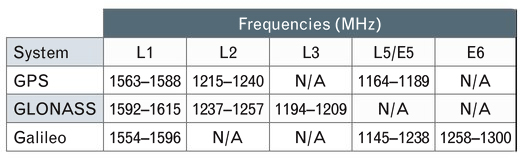
Frequency Coverage. GNSS receivers brought to market today may include frequency bands such as GPS L5, Galileo E5/E6, and the GLONASS bands in addition to the legacy GPS bands, and the antenna feeding a receiver may need to cover some or all of these bands.
TABLE 1 presents an overview of the frequencies used by the various GNSS constellations. Keep in mind that you may see slightly different numbers published elsewhere depending on how the signal bandwidths are defined.
TABLE 1. GNSS Frequency Allocations. (Data: Gerald J. K. Moernaut and Daniel Orban)
As the bandwidth requirement of an antenna increases, the antenna becomes harder to design, and developing an antenna that covers all of these bands and making it compliant with all of the other requirements is a challenge.
If small size is also a requirement, some level of compromise will be needed.
Gain Pattern. For a transmitting antenna, gain is the ratio of the radiation intensity in a given direction to the radiation that would be obtained if the power accepted by the antenna was radiated isotropically. For a receiving antenna, it is the ratio of the power delivered by the antenna in response to a signal arriving from a given direction compared to that delivered by a hypothetical isotropic reference antenna. The spatial variation of an antenna’s gain is referred to as the radiation pattern or the receiving pattern. Actually, under the antenna reciprocity theorem, these patterns are identical for a given antenna and, ignoring losses, can simply be referred to as the gain pattern.
The receiver operates best with only a small difference in power between the signals from the various satellites being tracked and ideally the antenna covers the entire hemisphere above it with no variation in gain. This has to do with potential cross-correlation problems in the receiver and the simple fact that excessive gain roll-off may cause signals from satellites at low elevation angles to drop below the noise floor of the receiver.
On the other hand, optimization for multipath rejection and antenna noise temperature (see below) require some gain roll-off.
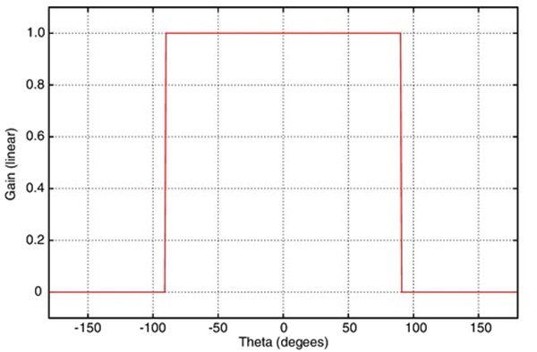
FIGURE 1. Theoretical antenna with hemispherical gain pattern. Boresight corresponds to θ = 0°. (Data: Gerald J. K. Moernaut and Daniel Orban)
FIGURE 1 shows what a perfect hemispherical gain pattern looks like, with a cut through an arbitrary azimuth.
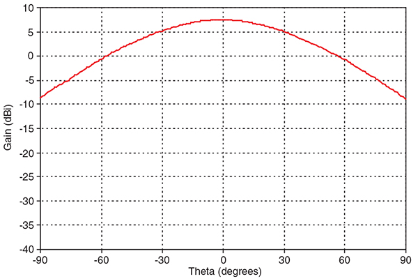
However, such an antenna cannot be built and “real-world” GNSS antennas see a gain roll-off of 10 to 20 dB from boresight (looking straight up from the antenna) to the horizon. FIGURE 2 shows what a typical gain pattern looks like as a cross-section through an arbitrary azimuth.
FIGURE 2. “Real-world” antenna gain pattern. (Data: Gerald J. K. Moernaut and Daniel Orban)
Circular Polarization. Spaceborne systems at L-Band typically use circular polarization (CP) signals for transmitting and receiving. The changing relative orientation of the transmitting and receiving CP antennas as the satellites orbit the Earth does not cause polarization fading as it does with linearly polarized signals and antennas. Furthermore, circular polarization does not suffer from the effects of Faraday rotation caused by the ionosphere. Faraday rotation results in an electromagnetic wave from space arriving at the Earth’s surface with a different polarization angle than it would have if the ionosphere was absent. This leads to signal fading and potentially poor reception of linearly polarized signals.
Circularly polarized signals may either be right-handed or left-handed. GNSS satellites use right-hand circular polarization (RHCP) and therefore a GNSS antenna receiving the direct signals must also be designed for RHCP.
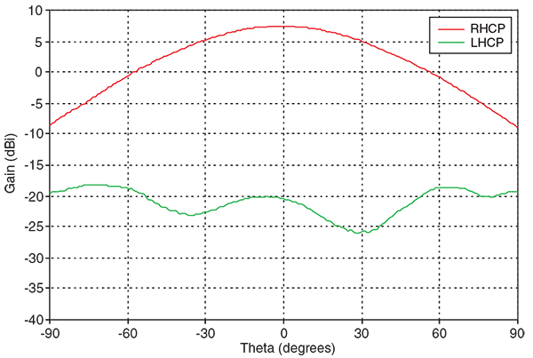
Antennas are not perfect and an RHCP antenna will pick up some left-hand circular polarization (LHCP) energy. Because GPS and other GNSS use RHCP, we refer to the LHCP part as the cross-polar component (see FIGURE 3).
FIGURE 3. Co- and cross-polar gain pattern versus boresight angle of a rover antenna. (Data: Gerald J. K. Moernaut and Daniel Orban)
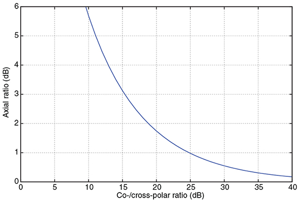
We can describe the quality of the circular polarization by either specifying the ratio of this cross-polar component with respect to the co-polar component (RHCP to LHCP), or by specifying the axial ratio (AR). AR is the measure of the polarization ellipticity of an antenna designed to receive circularly polarized signals. An AR close to 1 (or 0 dB) is best (indicating a good circular polarization) and the relationship between the co-/cross-polar ratio and axial ratio is shown in FIGURE 4.
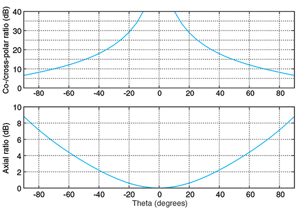
FIGURE 4. Converting axial ratio to co-/cross-polar ratio. (Data: Gerald J. K. Moernaut and Daniel Orban)FIGURE 5. Co-/cross-polar and axial ratios versus boresight angle of a rover-style antenna. (Data: Gerald J. K. Moernaut and Daniel Orban)
FIGURE 5 shows the ratio of the co- and cross-polar components and the axial ratio versus boresight (or depression) angle for a typical GPS antenna. The boresight angle is the complement of the elevation angle.
For high-end GNSS antennas such as choke-ring and other geodetic-quality antennas, the typical AR along the boresight should be not greater than about 1 dB. AR increases towards lower elevation angles and you should look for an AR of less than 3 to 6 dB at a 10° elevation angle for a high-performance antenna. Expect to see small (<1 dB) variations of AR versus azimuth at the low elevation angles.
Maintaining a good AR over the entire hemisphere and at all frequencies requires a lot of surface area in the antenna and can only be accomplished in high-end antennas like base station and rover antennas.
Multipath Suppression. Signals coming from the satellites arrive at the GNSS receiver’s antenna directly from space, but they may also be reflected off the ground, buildings, or other obstacles and arrive at the antenna multiple times and delayed in time. This is termed multipath. It degrades positioning accuracy and should be avoided. High-end receivers are able to suppress multipath to a certain extent, but it is good engineering practice to suppress multipath in the antenna as much as possible.
A multipath signal can come from three basic directions:
The ground and arrive at the back of the antenna.
The ground or an object and arrive at the antenna at a low elevation angle.
An object and arrive at the antenna at a high elevation angle.
Reflected signals typically contain a large LHCP component. The technique to mitigate each of these is different and, as an example, we will describe suppression of multipath signals due to ground and vertical object reflections.
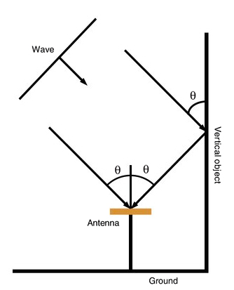
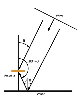
Multipath susceptibility of an antenna can be quantified with respect to the antenna’s gain pattern characteristics by the multipath ratio (MPR). FIGURE 6 sketches the multipath problem due to ground reflections.
FIGURE 6. Quantifying multipath caused by ground reflections. (Data: Gerald J. K. Moernaut and Daniel Orban)
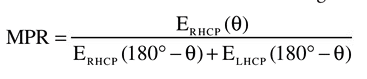
We can derive this MPR formula for ground reflections:
The MPR for signals that are reflected from the ground equals the RHCP antenna gain at a boresight angle (θ) divided by the sum of the RHCP and LHCP antenna gains at the supplement of that angle.
Signals that are reflected from the ground require the antenna to have a good front-to-back ratio if we want to suppress them because an RHCP antenna has by nature an LHCP response in the anti-boresight or backside hemisphere. The front-to-back ratio is nominally the difference in the boresight gain and the gain in the anti-boresight direction. A good front-to-back ratio also minimizes ground-noise pick-up.
Similarly, an MPR formula can be written for signals that reflect against vertical objects. FIGURE 7 sketches this.
FIGURE 7. Quantifying multipath caused by vertical object reflections. (Data: Gerald J. K. Moernaut and Daniel Orban)
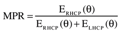
And the formula looks like this:
The MPR for signals that are reflected from vertical objects equals the RHCP antenna gain at a boresight angle (θ) divided by the sum of the RHCP and LHCP antenna gains at that angle.
Multipath signals from reflections against vertical objects such as buildings can be suppressed by having a good AR at those elevation angles from which most vertical object multipath signals arrive. This AR requirement is readily visible in the MPR formula considering these reflections are predominantly LHCP, and in this case MPR simply equals the co- to cross-polar ratio.
LHCP reflections that arrive at the antenna at high elevation angles are not a problem because the AR tends to be quite good at these elevation angles and the reflection will be suppressed. LHCP signals arriving at lower elevation angles may pose a problem because the AR of an antenna at low elevation angles is degraded in “real-world” antennas. It makes sense to have some level of gain roll-off towards the lower elevation angles to help suppress multipath signals. However, a good AR is always a must because gain roll-off alone will not do not it.
Phase Center. A position fix in GNSS navigation is relative to the electrical phase center of the antenna. The phase center is the point in space where all the rays appear to emanate from (or converge on) the antenna. Put another way, it is the point where the electromagnetic fields from all incident rays appear to add up in phase. Determining the phase center is important in GNSS applications, particularly when millimeter-positioning resolution is desired.
Ideally, this phase center is a single point in space for all directions at all frequencies. However, a “real-world” antenna will often possess multiple phase center points (for each lobe in the gain pattern, for example) or a phase center that appears “smeared out” as frequency and viewing angle are varied.
The phase-center offset can be represented in three dimensions where the offset is specified for every direction at each frequency band. Alternatively, we can simplify things and average the phase center over all azimuth angles for a given elevation angle and define it over the 10° to 90° elevation-angle range. For most applications even this simplified representation is over-kill, and typically only a vertical and a horizontal phase-center offset are specified for all bands in relation to L1.
For well-designed high-end GNSS antennas, phase center variations in azimuth are small and on the order of a couple of millimeters. The vertical phase offsets are typically 10 millimeters or less. Many high-end antennas have been calibrated, and tables of phase-center offsets for these antennas are available.
Impact on Receiver Sensitivity. The strength of the signals from space is on the order of -130 dBm. We need a really sensitive receiver if we want to be able to pick these up. For the antenna, this translates into the need for a high-performance low noise amplifier (LNA) between the antenna element itself and the receiver.
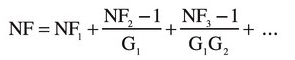
We can characterize the performance of a particular receiver element by its noise figure (NF), which is the ratio of actual output noise of the element to that which would remain if the element itself did not introduce noise. The total (cascaded) noise figure of a receiver system (a chain of elements or stages) can be calculated using the Friss formula as follows:
The total system NF equals the sum of the NF of the first stage (NF1) plus that of the second stage (NF2) minus 1 divided by the total gain of the previous stage (G1) and so on. So the total NF of the whole system pretty much equals that of the first stage plus any losses ahead of it such as those due to filters.
Expect to see total LNA noise figures in the 3-dB range for high performance GNSS antennas.
The other requirement for the LNA is for it to have sufficient gain to minimize the impact of long and lossy coaxial antenna cables — typically 30 dB should be enough. Keep in mind that it is important to have the right amount of gain for a particular installation. Too much gain may overload the receiver and drive it into non-linear behavior (compression), degrading its performance. Too little, and low-elevation-angle observations will be missed. Receiver manufacturers typically specify the required LNA gain for a given cable run.
Interference Handling. Even though GNSS receivers are good at mitigating some kinds of interference, it is essential to keep unwanted signals out of the receiver as much as possible. Careful design of the antenna can help here, especially by introducing some frequency selectivity against out-of-band interferers. The mechanisms by which in-band an out-of-band interference can create trouble in the LNA and the receiver and the approach to dealing with them are somewhat different.
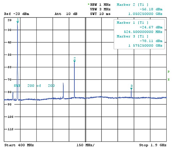
FIGURE 8. Strong out-of-band interferer and third harmonic in the GPS L1 band. (Data: Gerald J. K. Moernaut and Daniel Orban)
An out-of-band interferer is generally an RF source outside the GNSS frequency bands: cellular base stations, cell phones, broadcast transmitters, radar, etc. When these signals enter the LNA, they can drive the amplifier into its non-linear range and the LNA starts to operate as a multiplier or comb generator. This is shown in FIGURE 8 where a -30-dBm-strong interferer at 525 MHz generates a -78 dBm spurious signal or spur in the GPS L1 band.
Through a similar mechanism, third-order mixing products can be generated whereby a signal is multiplied by two and mixes with another signal. As an example, take an airport where radars are operating at 1275 and 1305 MHz. Both signals double to 2550 and 2610 MHz. These will in turn mix with the fundamentals and generate 1245 and 1335 MHz signals.
Another mechanism is de-sensing: as the interference is amplified further down in the LNA’s stages, its amplitude increases, and at some point the GNSS signals get attenuated because the LNA goes into compression. The same thing may happen down the receiver chain. This effectively reduces the receiver’s sensitivity and, in some cases, reception will be lost completely.
RF filters can reduce out-of-band signals by 10s of decibels and this is sufficient in most cases. Of course, filters add insertion loss and amplitude and phase ripple, all of which we don’t want because these degrade receiver performance.
In-band interferers can be the third-order mixing products we mentioned above or simply an RF source that transmits inside the GNSS bands. If these interferers are relatively weak, the receiver will handle them, but from a certain power level on, there is just not a lot we can do in a conventional commercial receiver.
The LNA should be designed for a high intercept point (IP)–at which non-linear behavior begins–so compression does not occur with strong signals present at its input. On the other hand, there is no requirement for the LNA to be a power amplifier. As an example, let’s say we have a single strong continuous wave interferer in the L1 band that generates -50 dBm at the input of the LNA. A 50 dB, high IP LNA will generate a 0 dBm carrier in the L1 band but the receiver will saturate.
LNAs with a higher IP tend to consume more power and in a portable application with a rover antenna — that may be an issue. In a base-station antenna, on the other hand, low current consumption should not be a requirement since a higher IP is probably more valuable than low power consumption.
GNSS Antenna Types
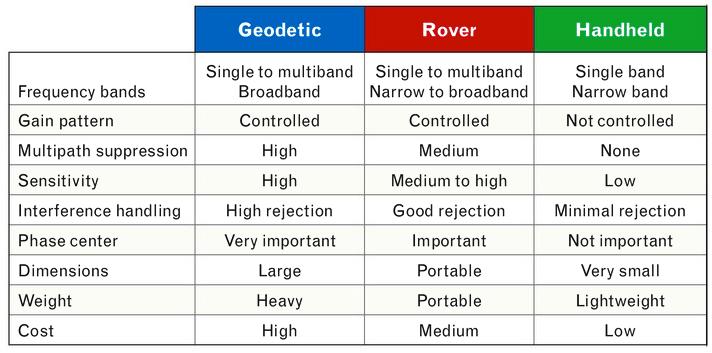
Here is a short comparison of three types of GNSS antennas: geodetic, rover, and handheld. For detailed specifications of examples of each of these types, see the references in Further Reading.
Geodetic Antennas. High precision, fixed-site GNSS applications require geodetic-class receivers and antennas. These provide the user with the highest possible position accuracy.
As a minimum, typical geodetic antennas cover the GPS L1 and L2 bands. Some also cover the GLONASS frequencies. Coverage of L5 is found in some newer designs as well as coverage of the Galileo frequencies and the L-band frequencies of differential GNSS services.
The use of choke-ring ground planes is typical in geodetic antennas. These allow good gain pattern control, excellent multipath suppression, high front-to-back ratio, and good AR at low elevation angles. Choke rings contribute to a stable phase center. The phase center is documented (as mentioned earlier), and high-end receivers allow the antenna behavior to be taken into account. Combined with a state-of-the-art LNA, these antennas provide the highest possible performance.
Rover Antennas. Rover antennas are typically used in land survey, forestry, construction, and other portable or mobile applications. They provide the user with good accuracy while being optimized for portability. Horizontal phase-center variation versus azimuth should be low because the orientation of the antenna with respect to magnetic north, say, is usually unknown and cannot be corrected for in the receiver. A rover antenna is typically mounted on a handheld pole. Good front-to-back ratio is required to avoid operator-reflection multipath and ground-noise pickup. Yet these rover-type applications are high accuracy and require a good phase-center stability. However, since a choke ring cannot be used because of its size and weight, a higher phase-center variation compared to that of a geodetic antenna is typically inherent to the rover antenna design.
A good AR and a decent gain roll-off at low elevation angles ensures good multipath suppression as heavy choke rings are not an option for this configuration.
Handheld Receiver Antennas. These antennas are single-band L1 structures optimized for size and cost. They are available in a range of implementations, such as surface mount ceramic chip, helical, and patch antenna types. Their radiation patterns are quasi-hemispherical. AR and phase-center performance are a compromise because of their small size. Because of their reduced size, these antennas tend to have a negative gain of about -3 dBi (3 dB less than an ideal isotropic antenna) at boresight. This negative gain is mostly masked by an embedded LNA. The associated elevated noise figure is typically not an issue in handheld applications.
TABLE 2. Characteristics of different GNSS antenna classes. (Data: Gerald J. K. Moernaut and Daniel Orban)
Summary of Antenna Types. TABLE 2 presents a comparison of the most important properties of geodetic, rover, and handheld types of GNSS antennas.
Conclusion
In this article, we have presented an overview of the most important characteristics of GNSS antennas. Several GNSS receiver-antenna classes were discussed based on their typical characteristics, and the resulting specification compromises were outlined. Hopefully, this information will help you select the right antenna for your next GNSS application.
Acknowledgment
An earlier version of this article entitled “Basics of GPS Antennas” appeared in The RF & Microwave Solutions Update, an online publication of RF Globalnet.
GERALD J. K. MOERNAUT holds an M.Sc. degree in electrical engineering. He is a full-time antenna design engineer with Orban Microwave Products, a company that designs and produces RF and microwave subsystems and antennas with offices in Leuven, Belgium, and El Paso, Texas.
DANIEL ORBAN is president and founder of Orban Microwave Products. In addition to managing the company, he has been designing antennas for a number of years.
FURTHER READING
Previous GPS World Articles on GNSS Antennas
“Getting into Pockets and Purses: Antenna Counters Sensitivity Loss in Consumer Devices” by B. Hurte and O. Leisten in GPS World, Vol. 16, No. 11, November 2005, pp. 34-38.
“Characterizing the Behavior of Geodetic GPS Antennas” by B.R. Schupler and T.A. Clark in GPS World, Vol. 12, No. 2, February 2001, pp. 48-55.
“A Primer on GPS Antennas” by R.B. Langley in GPS World, Vol. 9, No. 7, July 1998, pp. 50-54.
“How Different Antennas Affect the GPS Observable” by B.R. Schupler and T.A. Clark in GPS World, Vol. 2, No. 10, November 1991, pp. 32-36.
Introduction to Antennas and Receiver Noise
“GNSS Antennas and Front Ends” in A Software-Defined GPS and Galileo Receiver: A Single-Frequency Approach by K. Borre, D.M.Akos, N. Bertelsen, P. Rinder, and S.H. Jensen, Birkhäuser Boston, Cambridge, Massachusetts, 2007.
The Technician’s Radio Receiver Handbook: Wireless and Telecommunication Technology by J.J. Carr, Newnes Press, Woburn, Massachusetts, 2000.
“GPS Receiver System Noise” by R.B. Langley in GPS World, Vol. 8, No. 6, June 1997, pp. 40-45.
More on GNSS Antenna Types
“The Basics of Patch Antennas” by D. Orban and G.J.K. Moernaut. Available on the Orban Microwave Products website.
It is well known that the phase center of a GNSS antenna can vary with the satellite direction. This phase center movement leads to aspect dependent carrier phase and code phase biases in the satellite signal. For precise geo-location, one needs to characterize the antenna-induced carrier and code phase biases over the upper hemisphere. In the case of fixed pattern antennas (the antenna pattern does not vary with the incident signal environment) one can characterize the antenna induced biases a priori and use the data for corrections in the field. This is a standard practice in the surveying community.
For antennas used with AJ (Anti-Jam) systems, however, a priori characterization of the antenna induced biases may not be of much value. These antennas consist of multiple elements. The signals received by various antenna elements are weighted and then summed together to form the composite output signal. The element weights depend on the incident signal (mainly interfering signal) scenario. As the incident signal scenario changes so do the individual antenna element weights which in turn will lead to different values for antenna induced carrier phase and code phase biases.
As illustration, Figure 1 shows the antenna induced code phase bias of an AJ antenna over the upper hemisphere in the absence of all interfering signals as well as in the presence of two interfering signals.
Figure 1. Antenna induced code phase bias (in meters) over the upper hemisphere. Left: no interfering signal; right: two interfering signals.
In the figure, the center of the circle corresponds to the zenith and the outer ring corresponds to the horizon. The antenna induced code phase bias is plotted using a color scale in meters. Note that even in the absence of interfering signals, the antenna induced bias varies with the aspect angle. The presence of the interfering signals affects the antenna induced biases. This is true in the angular region surrounding the interfering signals as well as in the angular region away from the interfering signals.
One can observe this more clearly in Figure 2 where the difference between the antenna induced code phase biases in the absence of interfering signals and in the presence of interfering signals is plotted using a color scale in centimeters. Note that the difference in the antenna induced code phase bias is quite significant, and one may not be able to obtain precise location without proper corrections.
Figure 2. Difference (in cm) between the antenna-induced code phase bias in the presence of two interfering signals and in the absence of the interfering signals.
The question is what could be done to minimize the effects of adaptive antenna induced biases in GNSS receivers. In my opinion, one can take the following two approaches. In the first approach (see reference), one predicts the antenna-induced biases on the fly. This approach requires knowledge of in situ volumetric patterns of individual elements of an AJ antenna over the bandwidth of GNSS signals as well as access to the antenna element weights. With a perfect knowledge of these quantities, one can come up with a very good prediction and can correct for the antenna induced biases. The sensitivity of the prediction to various parameters, however, needs to be studied.
The second approach would be to develop novel weighting algorithms for GPS receiver adaptive antennas. Note that the current algorithms are mostly designed to either steer nulls in the interfering signal directions or maximize carrier to noise ratio in some sense. These novel algorithms should not only lead to improved carrier to noise ratio in the presence of interfering signals but should also make sure that the antenna-induced biases do not vary from their values in the absence of all interfering signals.
Further, these algorithms should not use many degrees of freedom to meet the various constraints in that GNSS AJ antennas do not have many degrees of freedom. If most of the degrees of freedom are consumed to meet the above constraints then one will not have enough degrees of freedom left to null the interfering signals. This is a very challenging task, but leads to a good research problem!
Inder J. Gupta
Ohio State University
References
I.J. Gupta, et. al., Prediction of antenna and antenna electronics induced biases in GNSS receivers, Proceedings of ION 2007 National Technical Meeting, San Diego, CA, January 2007.