Tag: algorithms and methods

Innovation: How Deep Is That White Stuff?

Using GPS Multipath for Snow-Depth Estimation

By Felipe G. Nievinski and Kristine M. Larson

INNOVATION INSIGHTS by Richard Langley

FRINGES. No, I’m not talking about the latest celebrity hairstyles nor the canopy of an American doorless, four-wheeled carriage from yesteryear (think Oklahoma!). I’m talking about interference fringes. But there is a connection to these other uses of the word fringe as we’ll see. You’ve all seen interference fringes at your local gas station, typically after it has just rained. They are the alternating bands of color we perceive when looking at a gasoline or oil slick in a puddle of water. They are caused by the white light from the Sun or artificial lighting reflected from the top surface of the slick and that from the bottom surface at the slick-water interface combining or interfering with each other at our eyeballs. The two sets of light waves arrive slightly out of phase with each other, and depending on the wavelengths of the reflected light and our angle of view, produce the colorful fringes. If the incident light was monochromatic, consisting of a single frequency or wavelength, then we would perceive just alternating bright and dark bands. The bright bands result from constructive interference when the phase difference is a near a multiple of 2π whereas the dark bands result from destructive interference when the difference is near an odd multiple of π.

Interference fringes had been seen long before the invention of the automobile. They are clearly seen on soap bubbles and the iridescent colors of peacock feathers, Morpho butterflies, and jewel beetles are also due to the interference phenomenon rather than pigmentation. Sir Isaac Newton did experiments on interference fringes (amongst other things) and tried to explain their existence — wrongly, it turned out. But he did coin the term fringes since they resembled the decorative fringe sometimes used on clothing, drapery, and, yes, surrey canopies.

It was the English polymath, Thomas Young, who, in 1801, first demonstrated interference as a consequence of the wave-nature of light with his famous double-slit experiment. You may have replicated his experiment in a high-school physics class. I did and I think I did it again as an undergraduate student taking a course in optics. Already by that point I was aiming for a career in physics or space science but I didn’t know that as a graduate student I would do research involving interference fringes. But not using light waves.

My research involved the application of very long baseline interferometry or VLBI to geodesy. VLBI had been developed by radio astronomers to better understand the structure of quasars and other esoteric celestial objects. At either ends of a baseline connecting large radio telescopes, perhaps stretching between continents, the quasar signals were recorded on magnetic tape and precisely registered using atomic clocks. When the tapes were played back and the signals aligned, one obtained interference fringes as peaks and troughs in an analog or digital waveform. Computer analysis of these fringes not only provided information on the structure of the observed radio source but also on the distance between the radio telescopes — eventually accurate enough to measure continental drift.

But what has all of this got to do with GPS? In this month’s column, we look at a technique that uses fringes generated by signals arriving at an antenna directly from GPS satellites and those reflected by snow surrounding the antenna to measure its depth and how it varies over time. GPS for measuring snow depth; who would have thought?

“Innovation” is a regular feature that discusses advances in GPS technology and its applications as well as the fundamentals of GPS positioning. The column is coordinated by Richard Langley of the Department of Geodesy and Geomatics Engineering, University of New Brunswick. He welcomes comments and topic ideas.

Snowpacks are a vital resource for human existence on our planet. They provide reservoirs of fresh water, storing solid precipitation and delaying runoff. One sixth of the world population depends on this resource. Both scientists and water-supply managers need to know how much fresh water is stored in snowpack and how fast it is being released as a result of melting.

Snow monitoring from space is currently under investigation by both NASA and ESA. Greatly complementary to such spaceborne sensors are automated ground-based methods; the latter not only serve as essential independent validation and calibration for the former, but are also valuable for climate studies and flood/drought monitoring on their own. It is desirable for such estimates to be provided at an intermediary scale, between point-like in situ samples and wider area pixels.

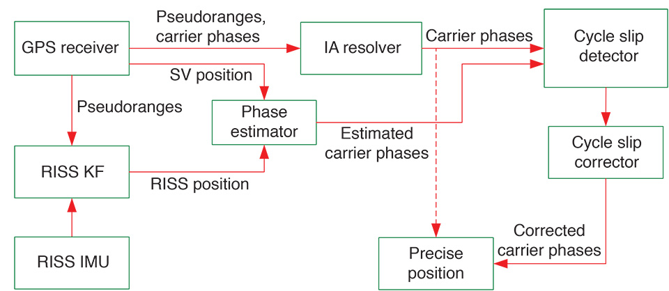
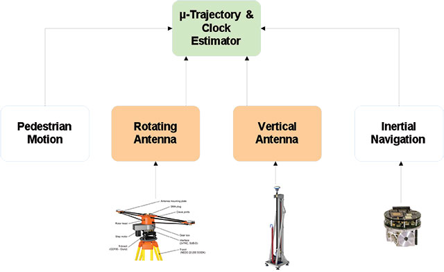
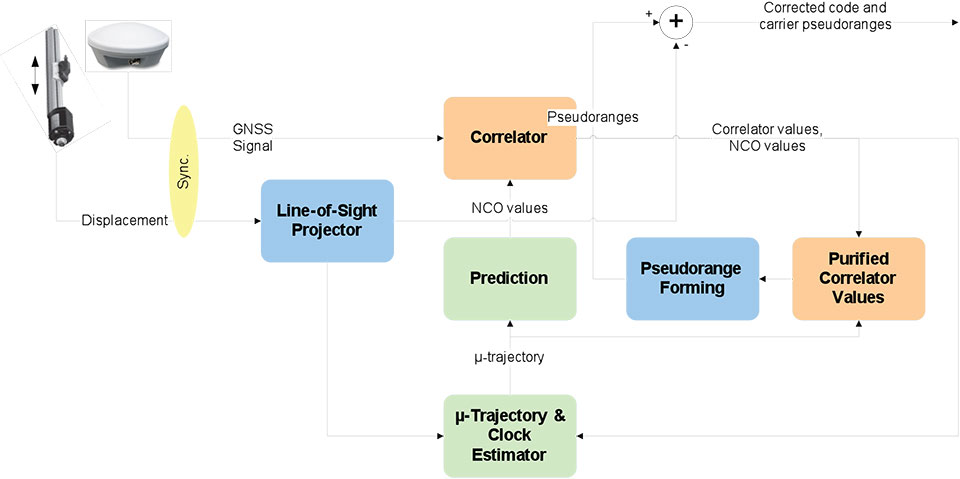
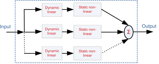
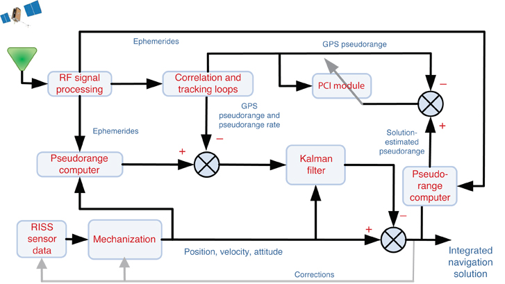
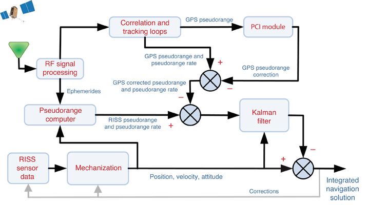
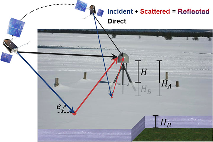
In the last decade, GPS multipath reflectometry (GPS-MR), also known as GPS interferometric reflectometry and GPS interference-pattern technique, has been proposed for monitoring snow. This method tracks direct GPS signals, those that travel directly to an antenna, that have interfered with a coherently reflected signal, turning the GPS unit into an interferometer (see FIGURE 1). Its main variant is based on signal-to-noise ratio (SNR) measurements, although GPS-MR is also possible with carrier-phase and pseudorange observables. Data are collected at existing GPS base stations that employ commercial-off-the-shelf receivers and antennas in a conventional, antenna-upright setup. Other researchers have used a custom antenna and/or a dedicated setup, with the antenna tipped for enhanced multipath reception.

FIGURE 1. Standard geodetic receiver installation. The antenna is protected by a hemispherical radome. The monument (tripod structure) is ~ 2 meters above the ground. GPS satellites rise and set in ascending and descending sky tracks, multiple times per day. The specular reflection point migrates radially away from the receiver for decreasing satellite elevation angle. The total reflector height is made up of an a priori value and an unknown bias driven by the thickness of the snow layer.

In this article, we summarize the SNR-based GPS-MR technique as applied to snow sensing using geodetic instruments. This forward/inverse approach for GPS-MR is new in that it capitalizes on known information about the antenna response and the physics of surface scattering to aid in retrieving the unknown snow conditions in the site surroundings. It is a statistically rigorous retrieval algorithm, agreeing to first order with the simpler original methodology, which is retained here for the inversion bootstrapping. The first part of the article describes the retrieval algorithm, while the second part provides validation at a representative site over an extended period of time.

Physical Forward Model

SNR observations are formulated as SNR = P_s/P_n. In the denominator, we have the noise power, P_n, here taken as a constant, based on nominal values for the noise power spectral density and the noise bandwidth. The numerator is composite signal power:

. (1)

Its incoherent component is the sum of the respective direct and reflected powers (although direct incoherent power is negligible). In contrast, the coherent composite signal power follows from the complex sum of direct and reflection average voltages (not to be confused with the electromagnetic propagating fields, which neglect the receiving antenna response and also the receiver tracking process):

(2)

It is expressed in terms of the coherent direct and reflected powers, as well as the interferometric phase,

, (3)

which amounts to the reflection excess phase with respect to the direct signal.

We decompose observations, SNR = tSNR + dSNR, into a trend

(4)

over which interference fringes are superimposed:

. (5)

From now on, we neglect the incoherent power, which only impacts tSNR, not dSNR, and drop the coherent power superscript, for brevity.

The direct or line-of-sight power is formulated as

(6)

where is the direction-dependent right-hand circularly polarized (RHCP) power component incident on an isotropic antenna; the left-handed circularly polarized (LHCP) component is negligible. The direct antenna gain, , is obtained evaluating the antenna pattern in the satellite direction and with RHCP polarization.

The reflection power,

, (7)

is defined starting with the same incident isotropic power, , as in the direct power. It ends with a coherent power attenuation factor,

(8)

where θ is the angle of incidence (with respect to the surface normal), k = 2π/λ, is the wave number, and λ = 24.4 centimeters is the carrier wavelength for the civilian GPS signal on the L2 frequency (L2C). This polarization-independent factor accounts only for small-scale residual height above and below a large-scale trend surface. The former/latter results from high-/low-pass filtering the actual surface heights using the first Fresnel zone as a convolution kernel, roughly speaking. Small-scale roughness is parameterized in terms of an effective surface standard deviation s (in meters); its scattering response is modeled based on the theories of random surfaces, except that the theoretical ensemble average is replaced by a sensing spatial average. Large-scale deterministic undulations could be modeled, but their impact on snow depth is canceled to first-order by removing bare-ground reflector heights.

At the core of , we have coupled surface/antenna reflection coefficients, , producing respectively RHCP and LHCP fields (under the assumption of a RHCP incident field). These terms include antenna response power gain and phase patterns, evaluated in the reflection direction, and separately for each polarization. The surface response is represented by complex-valued Fresnel coefficients for cross- and same-sense circular polarization, respectively. The medium is assumed to be homogeneous (that is, a semi-infinite half-space). Material models provide the complex permittivity, which drives the Fresnel coefficients.

The interferometric phase reads:

.(9)

The first term accounts for the surface and antenna properties of the reflection, as above. The last one is the direct phase contribution, which amounts to only the RHCP antenna phase-center variation evaluated in the satellite direction. The majority of the components present in the direct RHCP phase (such as receiver and satellite clock states, the bulk of atmospheric propagation delays, and so on) are also present in the reflection phase, so they cancel out in forming the difference.

At the core of the interferometric phase, we have the geometric component, φ_I = kτ_i, the product of the wave number and the interferometric propagation delay. Assuming a locally horizontal surface, the latter is simply:

(10)

in terms of the satellite elevation angle, e, and an a priori reflector height, H_A. Snow depth will be measured in terms of changes in reflector height.

The physical forward model, based only on a priori information, can then be summarized as:

(11)

where interferometric power and phase are, respectively:

(12)

. (13)

In all of these terms the pseudorandom-noise-code modulation impressed on the carrier wave can be safely neglected, given the small interferometric delay and Doppler shift at grazing incidence, stationary surface/receiver conditions, and short antenna installations.

Parameterization of Unknowns

There are errors in the nominal values assumed for the physical parameters of the model (permittivity, surface roughness, reflector height, and so on). Ideally we would estimate separate corrections for each one, but unfortunately many are linearly dependent or nearly so. Because of this dependency, we have kept physical parameters fixed to their optimal a priori values, and have estimated a few biases. Each bias is an amalgamation of corrections for different physical effects. In a later stage, we rely on multiple independent bias estimates (such as for successive days) to try and separate the physical sources.

Each satellite track is inverted independently. A track is defined by partitioning the data by individual satellite and then into ascending and descending portions, splitting the period between the satellite’s rise and set at the near-zenith culmination. Each satellite track has a duration of ~1–2 hours. This configuration normally offers a sufficient range of elevation angles, unless the satellite reaches culmination too low in the sky (less than about 20°), in which case the track is discarded. In seeking a balance between under- and over-fitting, between an insufficient and an excessive number of parameters, we estimate the following vector of unknown parameters:

. (14)

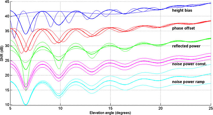
FIGURE 2 shows the effect of the constant and linear biases on the SNR observations. Reflector height bias, H_B , changes the number of oscillations; phase shift, φ_B , displaces the oscillations along the horizontal axis; reflection power, , affects the depth of fades; zeroth-order noise power, , shifts the observations up or down as a whole; and first-order noise power, , tilts the SNR curve. A good parameterization yields observation sensitivity curves as unique as possible for each parameter.

FIGURE 2. Effect of each parameter on SNR observations; curves are displaced vertically (6 dB) for clarity.

The forward model, now including the biases, can be summarized as follows:

(15)

where the modified interferometric power and phase are given by:

, (16)

. (17)

The total reflector height, H = H_A – H_B (a priori value minus unknown bias), is to be interpreted as an effective value that best fits measurements, which includes snow and other components.

Bootstrapping Parameter Priors. Biases and SNR observations are involved non-linearly through the forward model. Therefore, there is the need for a preliminary global optimization, without which the subsequent final local optimization will not necessarily converge to the optimal solution.

SNR observations would trace out a perfect sinusoid curve in the case of an antenna with isotropic gain and spherical phase pattern, surrounded by a smooth, horizontal, and infinite surface (free of small-scale roughness, large-scale undulations, and edges), made of perfectly electrically conducting material, and illuminated by constant incident power. Thus, in such an idealized case, SNR could be described exactly by constant reflector height, phase shift, amplitude, and mean values.

As the measurement conditions become more complicated, the SNR data start to deviate from a pure sinusoid. Yet a polynomial/spectral decomposition is often adequate for bootstrapping purposes.

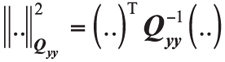
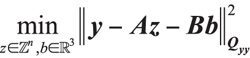
Statistical Inverse Model Formulation

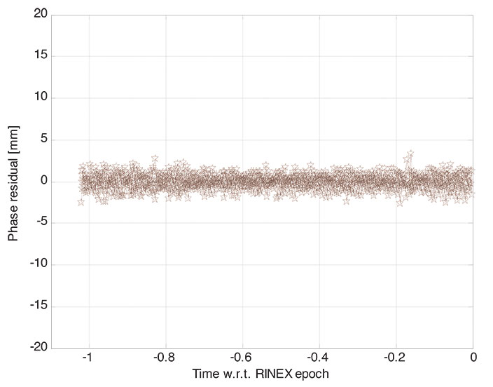
Based on the preliminary values for the unknown parameters vector and other known (or assumed) values, we run the forward model to obtain simulated observations. We form pre-fit residuals comparing the model values to SNR measurements collected at varying satellite elevation angles (separately for each track). Residuals serve to retrieve parameter corrections, such that the sum of squared post-fit residuals is minimized. This non-linear least squares problem is solved iteratively using both a functional model and a stochastic model. The functional modeling includes a Jacobian matrix of partial derivatives, which represents the sensitivity of observations to parameter changes where the partial derivatives are defined element-wise. Instead of deriving analytical expressions, we evaluate them numerically, via finite differencing. The stochastic model specifies the uncertainty and correlation expected in the residuals. Their a priori covariance matrix modifies the objective function being minimized.

Directional Dependence

It is important to know at which elevation angles the parameter estimates are best determined. Here, we focus on the phase parameters instead of reflection power or noise power parameters.

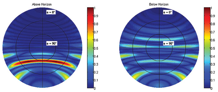
We can utilize the estimated reflector height and phase shift to evaluate the full phase bias function over varying elevation angles. Similarly, we can extract the corresponding 2-by-2 portion of the parameters’ a posteriori covariance matrix, containing the uncertainty for reflector height and for phase shift, as well as their correlation, which is then propagated to obtain the full phase uncertainty (see FIGURE 3).

FIGURE 3. Uncertainty of full phase function, propagated from the uncertainty of reflector height and of phase shift, as well as their correlation.

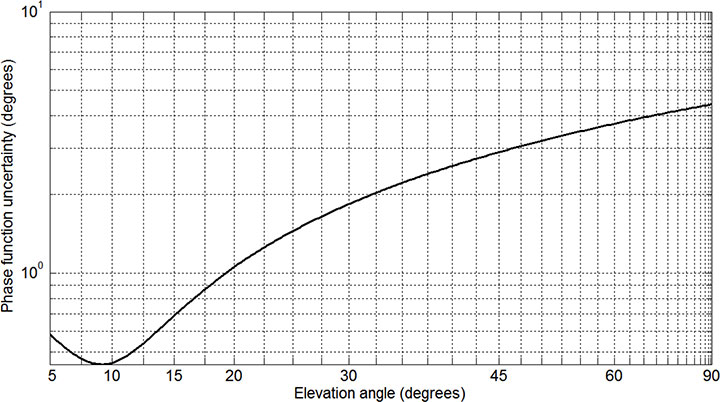
The uncertainty attains a clear minimum versus elevation angle. The least-uncertainty elevation angle pinpoints the observation direction where reflector height and phase shift are best determined (in combined form, not individually). The azimuth and epoch coinciding with the peak elevation angle act as track tags, later used for clustering similar tracks and analyzing their time series of retrievals.

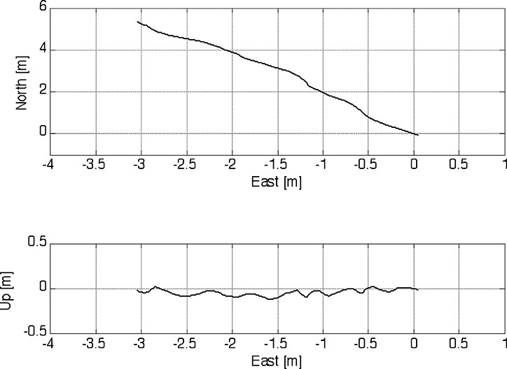
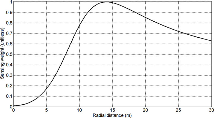
If we normalize phase uncertainty by its value at the peak elevation angle, then plot such sensing weights (between 0 and 1) versus the radial or horizontal distance to the center of the first Fresnel zone at each elevation angle, we obtain FIGURE 4. It can be interpreted as the reflection footprint, indicating the importance of varying distances, with a longer far tail and a shorter near tail (respectively regions beyond and closer than the peak distance). The implications for in situ data collection are clear: one should sample more intensely near the peak distance (about 15 meters) and less so in the immediate vicinity of the GPS antenna, tapering it off gradually away from the antenna. As a caveat, these conclusions are not necessarily valid for antenna setups other than the one considered here.

FIGURE 4. Reflection footprint in terms of a sensing weight (between 0 and 1) defined as the normalized reciprocal of full phase uncertainty, plotted versus the radial or horizontal distance from the receiving antenna to the center of the first Fresnel zone at each elevation angle; valid for an upright 2-meter-tall antenna; the receiving antenna is at zero radial distance.

Results

We now examine the snow-depth retrievals from the GPS multipath retrieval algorithm and assess both the precision and accuracy of the method. Multiple metrics have been developed to assess the quality of the results. The accuracy of the method has been evaluated by comparing with in situ data over a multi-year period. Three field sites were chosen to highlight different limitations in the method, both in terms of terrain and forest cover: grassland, alpine, and forested. We will look at the forested site in some detail.

Satellite Coverage and Track Clustering. All GPS-MR retrievals reported here are based on the newer GPS L2C signal. Of the approximately 30 GPS satellites in service, 8-10 L2C satellites were available between 2009 and 2012 (8, 9, and 10 satellites at the end of 2009, 2010, and 2011, respectively). Satellite observations were partitioned into ascending and descending portions, yielding approximately twenty unique tracks per day at a site with good sky visibility. GPS orbits are highly repeatable in azimuth, with deviations at the few-degree range over a year, translating into ~50-100-centimeter azimuthal displacement of the reflecting area (corresponding to the first Fresnel zone at 10°-15° elevation angle for a 2-meter high antenna). This repeatability permits clustering daily retrievals by azimuth. It also allows the simplification that estimated snow-free reflector heights are fairly consistent from day to day, facilitating the isolation of the varying snow depth during the snow-covered period.

For a given track, its revisit time is also repeatable, amounting to practically one sidereal day. The deficit in time relative to a calendar day results in the track time of the day receding ~4 minutes and 6 seconds every day. This slow but steady accumulation eventually makes the time of day return to its starting value after about one year. As all GPS satellites drift approximately at the same rate, the time between successive tracks remains nearly repeatable. Its reciprocal, the sampling rate, has a median equal to approximately one track per hour, with a low value of one track within two hours and a high of one track within 15 minutes; both extremes occur every day, with low-rate idle periods interspersed with high-rate bursts. The time of the day reduced to a fixed day (such as January 1, 2000) could also be used to cluster tracks. Neighboring clusters, which are close in azimuth and/or in reduced time of the day, are expected to be more comparable, as they sample similar conditions and are subject to similar errors.

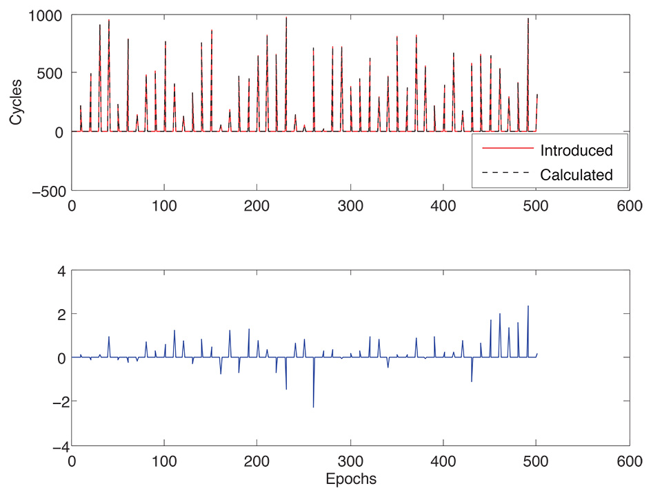
Observations. FIGURE 5 shows several representative examples of SNR observations. A typical good fit between measured and modeled values is shown in Figure 5(a), corresponding to the beginning of the snow season. Generally the model/measurement fit is good when the scattering medium is homogeneous; it deteriorates as the medium becomes more heterogeneous, particularly with mixtures of soil, snow, and vegetation. There are genuine physical effects as well as more mundane spurious instrumental issues that degrade the fit but do not necessarily cause a bias in snow-depth estimates. These include secondary reflections, interferometric power effects, direct power effects, and instrument-related issues.

FIGURE 5. Examples of observations: (a) good fit; (b) presence of secondary reflections; (c) vanishing interference fringes; (d) atypical interference fringes.

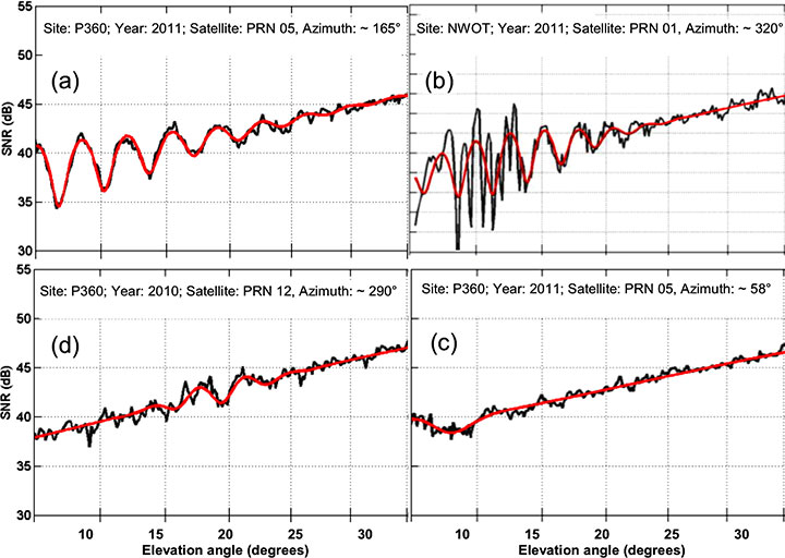
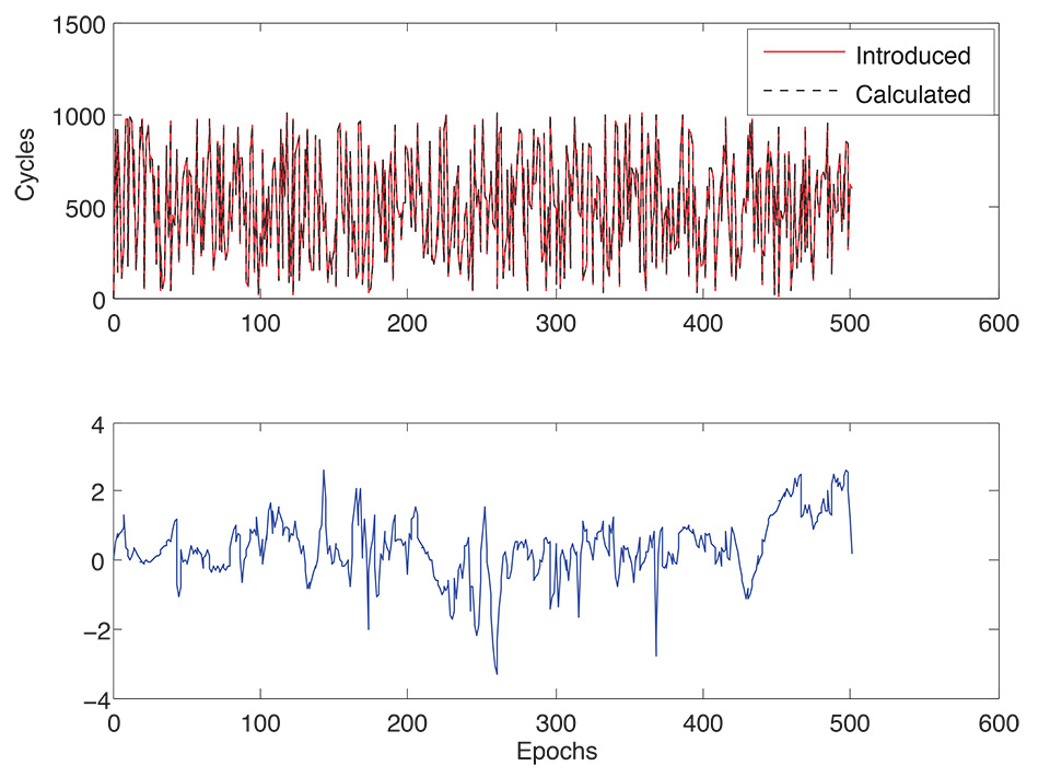
Secondary reflections originate from disjoint surface regions. Interference fringes become convoluted with multiple superimposed beats (see Figure 5(b)). As long as there is a unique dominating reflection, the inversion will have no difficulty fitting it, as the extra reflections will remain approximately zero-mean.

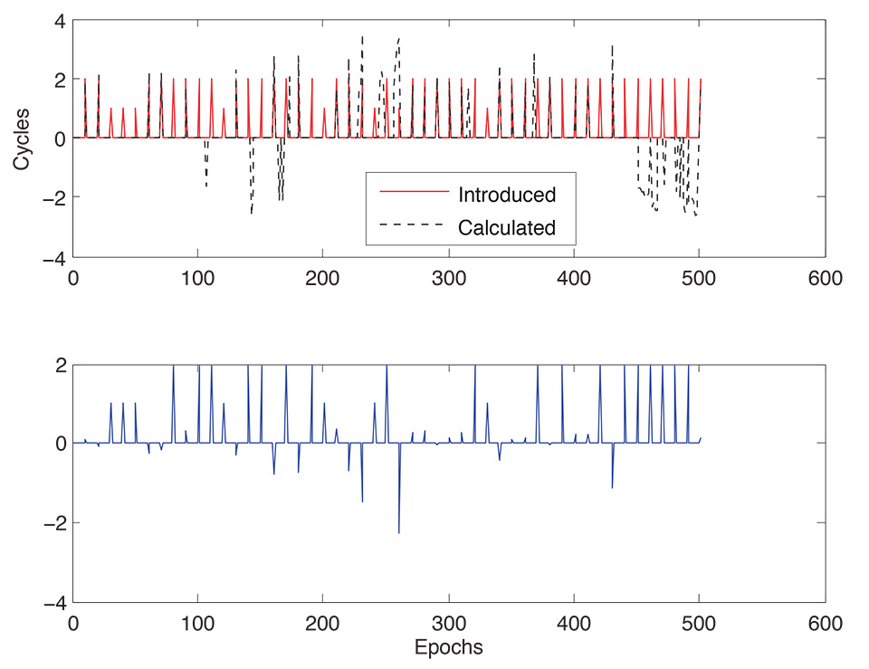
Random deviations of the actual surface with respect to its undulated approximation, called roughness or residual surface height, will affect the interferometric power. SNR measurements will exhibit a diminishing number of significant interference fringes, compared to the measurement noise level (see Figure 5(c)). This facilitates the model fit but the reflector height parameter may become ill-determined: its estimates will be more uncertain. Changes in snow density also affect the fringe amplitude.

Snow precipitation attenuates the satellite-to-ground radio link, which affects SNR measurements through the direct power term. First, this shifts the SNR measurements up or down (in decibels); second, it tilts the trend tSNR as attenuation is elevation-angle dependent; third, fringes in dSNR will change in amplitude because of the decrease in the coherent component of the direct power.

Partial obstructions can affect either or both direct and interferometric powers. In this case, SNR measurements, albeit corrupted, are still recorded. This situation is in contrast to complete blockages as caused by topography. The deposition of snow and the formation of a winter rime on the antenna are a particularly insidious type of obstruction, as their presence in the near-field of the antenna element can easily distort the gain pattern in a significant manner. In the far-field, trees are another important nuisance, so much so that their absence is held as a strong requirement for the proper functioning of multipath reflectometry.

Satellite-specific direct power offsets and also long-term power drifts are to be expected as spacecraft age and modernized designs are launched. In addition, noise power depends on the state of conservation of receiver cables and on their physical temperature. Less subtle incidents are sudden ~3-dB SNR steps, hypothesized to originate in the receiver switching between the L2C data and pilot subcodes, CM and CL.

Quality Control. Anomalous conditions may result in measurement spikes, jumps, and short-lived rapidly-varying fluctuations. For snow-depth-sensing purposes, it is necessary and sufficient to either neutralize such measurement outliers through a statistically robust fit or detect unreliable fits and discard the problematic ones that could not otherwise be salvaged.

The key to quality control (QC) is in grouping results into statistically homogeneous units, having measurements collected under comparable conditions. In our case, azimuth-clustered tracks are the natural starting unit. Secondarily, we must account for genuine temporal variations in the tendency of results, from beginning to peak to the end of the snow season. The detection of anomalous results further requires an estimate of the statistical dispersion to be expected. Considering that the sample is contaminated with outliers, robust estimators (running median instead of the running mean, and median absolute deviation over the standard deviation) are called for, if the first- and second-order statistical moments are to be representative. Given estimates of the non-stationary tendency and dispersion, a tolerance interval can then be constructed such that it bounds, say, a 99% proportion of the valid results with 95% confidence level. We also desire QC to be judicious, or else too many valid estimates will be lost. Notice that in the present intra-cluster QC, we compare an individual estimate to the expected performance of the track cluster to which it belongs; later, we complement QC with an inter-cluster comparison of each cluster’s own expected performance.

Based on our practical experience, no single statistic detects all the outliers. We use four particular statistics that we have found to be useful: 1) degrees of freedom, essentially the number of observations per track (modulo a constant number of parameters); 2) using the scaled root-mean-square error (RMSE) to test for goodness-of-fit, that is, how well measurements can be explained adjusting the unknown values for the parameters postulated in the model; 3) reflector height uncertainty; and 4) peak elevation angle, which behaves much like a random variable, as it is determined by a multitude of factors.

Combinations. We combine multiple clusters to average out random noise. Noise mitigation aims at not only coping with measurement errors but also compensating for model deficiencies, to the extent that they are not in common across different clusters. Before we combine different clusters, we have to address their long-term differences. The initial situation is that snow surface heights will be greater downhill and smaller uphill; we take this into account on a cluster-by-cluster basis by subtracting ground heights from their respective snow surface heights, resulting in snow thickness values, which is a completely physically unambiguous quantity. Snow thickness is more comparable than snow heights across varying-azimuth track clusters. Yet snow tends to fill in ground depressions, so thickness exhibits variability caused by the underlying ground surface, even when the overlying snow surface is relatively uniform. Further cluster homogeneity can be achieved by accounting for the temporally permanent though spatially non-uniform component of snow thickness.

The averaging of snow depths collected for different track clusters employs the inversion uncertainties to obtain a preliminary running weighted median, calculated for, say, daily postings, with overlapping windows or not. The preliminary post-fit residuals then go through their own averaging, necessarily employing a wider averaging window (say, monthly), which produces scaling factors for the original uncertainties. The running weighted median is then repeated, producing final averages. The variance factors reflect the fact that some clusters are better than others.

Thus, the final GPS estimates of snow depth follow from an averaging of all available tracks, whose individual snow depth values were previously estimated independently. A new average is produced twice daily utilizing the surrounding 1–2 days of data (depending on the data density), that is, 12-hour posting spacing and 24-hour moving window width. The averaging interval must be an integer number of days, so as to minimize the possibility of snow-depth artifacts caused by variations in the observation geometry, which repeats daily.

Site-Specific Results

We explored GPS-MR snow-depth retrieval at three stations over a long period (up to three years). Throughout, we assessed the performance of the GPS estimates against independent nearly co-located in situ measurements. We also compared the GPS estimates to the nearest SNOTEL station. SNOTEL (from snowpack telemetry) is an automated system for collecting snowpack and related data in the western U.S. operated by the U.S. Department of Agriculture. Although not co-located with GPS, SNOTEL data are important because they provide accurate information on the timing of snowfall events.

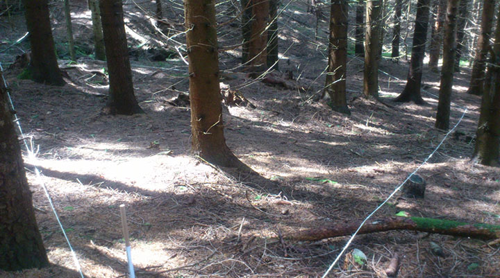
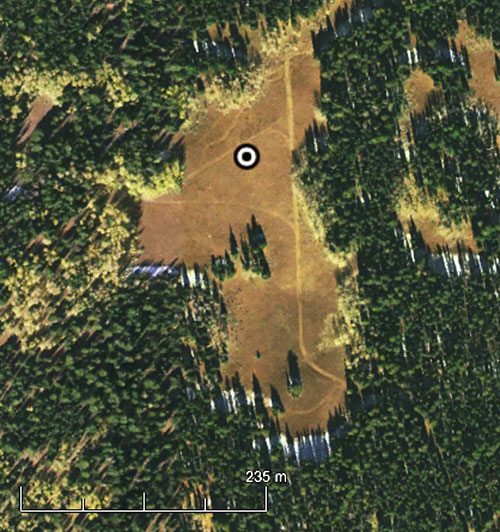
The three sites we used were 1) a site in the T.W. Daniel Experimental Forest within the Wasatch Cache National Forest in the Bear River Range of northeastern Utah, with an elevation of 2,600 meters; 2) one of the stations of the EarthScope Plate Boundary Observatory, a grassland site located near Island Park, Idaho; and 3) an alpine site in the Niwot Ridge Long-term Ecological Research Site near Boulder, Colorado. While we have fully documented the results from each site, due to space limitations we will only discuss the results from the forested site (known as RN86) in this article. This is a more challenging site than the other two, due to the presence of nearby trees. Furthermore, it was subject to denser in situ sampling of 20-150 measurements spatially replicated around the GPS antenna, and repeated approximately every other week for about one year.

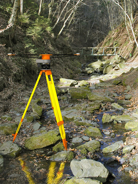
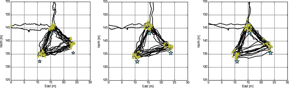
We show results for the 2012 water-year, the period starting October 1 through September 30 of the following year. Where GPS site RN86 was installed, topographical slopes range from 2.5° to 6.5° (at the 2-meter spatial scale), with average of ~5° within a 50-meter radius around the GPS antenna. RN86 was specifically built to study the impact of trees on GPS snow depth retrievals (see FIGURE 6). Ground crews manually collected in situ measurements around the GPS antenna approximately every other week starting in November 2011. Measurements were made every 1–2 meters from the antenna up to a distance of 25-30 meters. In the second half of the year, the sampling protocol was changed to azimuths of 0° (N), 45° (NE), 135° (SE), 180° (S), 225° (SW), and 315° (NW). With these data it is possible to obtain in situ average estimates, with their own uncertainties (based on the number of measurements), which allows a more meaningful comparison.

FIGURE 6. Aerial view of the forested site (RN86) around the GPS antenna (marked with a circle).

There is reduced visibility at the current site, compared to other sites. Track clusters are concentrated due south, with only two clusters located within ±90° of north. Therefore, the GPS average snow depth is not necessarily representative of the azimuthally symmetric component of the snow depth. In the presence of an azimuthal asymmetry in the snow distribution around the antenna, the GPS average would be expected to be biased towards the environmental conditions prevalent in the southern quadrant. To rule out the possibility of an azimuthal artifact in the comparisons, we have utilized only the in situ data collected along the SE/S/SW quadrant.

The comparison shows generally excellent agreement between GPS and in situ data (see FIGURE 7). The first four and the last one in situ data points were collected with coarser spacing and/or smaller azimuthal coverage, which may be partially responsible for different performance in the first and second halves of the snow season. The correlation between GPS and in situ snow depth at RN86 amounts to 0.990, indicating a very strong linear relationship. Carrying out a regression between in situ and GPS values, the RMS of snow-depth residuals improves from 9.6 to 3.4 centimeters. The regression intercept and slope (with corresponding 95% uncertainties) amount to 15.4 ± 9.11 centimeters and 0.858 ± 0.09 meters per meter, respectively. According to these statistics, the null hypotheses of zero intercept and unity slope are rejected at the 95% confidence level. This implies that at this location GPS snow-depth estimates exhibit both additive and multiplicative biases. The latter is proportional to snow depth itself, meaning that, compared to an ideal one-to-one relationship, GPS is found to under-estimate in situ snow depth at this site by 14 ± 9%, although the uncertainty is somewhat large.

FIGURE 7. Snow-depth measurement at the forested site (RN86) for the water-year 2012

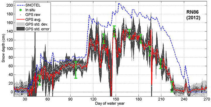
The SNOTEL sensors are exceptionally close to the GPS antenna at this site, about 350 meters horizontally distant with negligible vertical separation. Yet the former is located within trees, while the latter is located at the periphery of the forest and senses the reflections scattered from an open field. Therefore, only the timing of snowfall events agrees well, not the amount of snow. Although forest density is generally negatively correlated with snow depth, exceptions are not uncommon, especially in localized clearings exposed to intense solar radiation, where shading of the snow by the trees reduces ablation.

Conclusions

In this article, we have discussed a physically based forward model and a statistical inverse model for estimating snow depth based on GPS multipath observed in SNR measurements. We assessed model performance against independent in situ measurements and found they validated the GPS estimates to within the limitations of both GPS and in situ measurement errors after the characterization of systematic errors. The assessment yielded a correlation of 0.98 and an RMS error of 6–8 centimeters for observed snow depths of up to 2.5 meters at three sites, with the GPS underestimating in situ snow depth by ~5–15%. This latter finding highlights the necessity to assess effects currently neglected or requiring more precise modeling.

Acknowledgments

The research reported in this article was supported by grants from the U.S. National Science Foundation, NASA, and the University of Colorado. Nievinski has been supported by a Capes/Fulbright Graduate Student Fellowship and a NASA Earth System Science Research Fellowship. The article is based, in part, on two papers published in the IEEE Transactions on Geoscience and Remote Sensing: “Inverse Modeling of GPS Multipath for Snow Depth Estimation – Part I: Formulation and Simulations” and “Inverse Modeling of GPS Multipath for Snow Depth Estimation – Part II: Application and Validation.”

Manufacturers

For the forested site (RN86), a Trimble NetR9 receiver was used with a Trimble TRM57971.00 (Zephyr Geodetic II) antenna with no external radome.

FELIPE G. NIEVINSKI is a faculty member at the Federal University of Santa Catarina, Florianópolis, Brazil. He has also been a post-doctoral researcher at São Paulo State University, Presidente Prudente, Brazil. He earned a B.E. in geomatics from the Federal University of Rio Grande do Sul, Porto Alegre, Brazil, in 2005; an M.Sc.E. in geodesy from the University of New Brunswick, Fredericton, Canada, in 2009; and a Ph.D. in aerospace engineering sciences from the University of Colorado, Boulder, in 2013. His Ph.D. dissertation was awarded The Institute of Navigation Bradford W. Parkinson Award in 2013.

KRISTINE M. LARSON received a B.A. degree in engineering sciences from Harvard University and a Ph.D. degree in geophysics from the Scripps Institution of Oceanography, University of California at San Diego. She was a member of the technical staff at the Jet Propulsion Lab from 1988 to 1990. Since 1990, she has been a professor in the Department of Aerospace Engineering Sciences, University of Colorado, Boulder.

FURTHER READING

• Authors’ Journal Papers

“Inverse Modeling of GPS Multipath for Snow Depth Estimation—Part I: Formulation and Simulations” by F.G. Nievinski and K.M. Larson in IEEE Transactions on Geoscience and Remote Sensing, Vol. 52, No. 10, 2014, pp. 6555–6563, doi: 10.1109/TGRS.2013.2297681.

“Inverse Modeling of GPS Multipath for Snow Depth Estimation—Part II: Application and Validation” by F.G. Nievinski and K.M. Larson in IEEE Transactions on Geoscience and Remote Sensing, Vol. 52, No. 10, 2014, pp. 6564–6573, doi: 10.1109/TGRS.2013.2297688.

• More on the Use of GPS for Snow Depth Assessment

“Snow Depth, Density, and SWE Estimates Derived from GPS Reflection Data: Validation in the Western U.S.” by J.L. McCreight, E.E. Small, and K.M. Larson in Water Resources Research, published first on line, August 25, 2014, doi: 10.1002/2014WR015561.

“Environmental Sensing: A Revolution in GNSS Applications” by K.M. Larson, E.E. Small, J.J. Braun, and V.U. Zavorotny in Inside GNSS, Vol. 9, No. 4, July/August 2014, pp. 36–46.

“Snow Depth Sensing Using the GPS L2C Signal with a Dipole Antenna” by Q. Chen, D. Won, and D.M. Akos in EURASIP Journal on Advances in Signal Processing, Special Issue on GNSS Remote Sensing, Vol. 2014, Article No. 106, 2014, doi: 10.1186/1687-6180-2014-106.

“GPS Snow Sensing: Results from the EarthScope Plate Boundary Observatory” by K.M. Larson and F.G. Nievinski in GPS Solutions, Vol. 17, No. 1, 2013, pp. 41–52, doi: 10.1007/s10291-012-0259-7.

• GPS Multipath Modeling and Simulation

“Forward Modeling of GPS Multipath for Near-Surface Reflectometry and Positioning Applications” by F.G. Nievinski and K.M. Larson in GPS Solutions, Vol. 18, No. 2, 2014, pp. 309–322, doi: 10.1007/s10291-013-0331-y.

“An Open Source GPS Multipath Simulator in Matlab/Octave” by F.G. Nievinski and K.M. Larson in GPS Solutions, Vol. 18, No. 3, 2014, pp. 473–481, doi: 10.1007/s10291-014-0370-z.

“Multipath Minimization Method: Mitigation Through Adaptive Filtering for Machine Automation Applications” by L. Serrano, D. Kim, and R.B. Langley in GPS World, Vol. 22, No. 7, July 2011, pp. 42–48.

“It’s Not All Bad: Understanding and Using GNSS Multipath” by A. Bilich and K.M. Larson in GPS World, Vol. 20, No. 10, October 2009, pp. 31–39.

“GPS Signal Multipath: A Software Simulator” by S.H. Byun, G.A. Hajj, and L.W. Young in GPS World, Vol. 13, No. 7, July 2002, pp. 40–49.

September 1, 2014
Canadian Science Minister Announces Grant to Langley’s UNB Lab

Professor Langley (fourth from left) discusses the UNB geodesy program with Canadian Science Minister Ed Holder (third from left.)

The Canadian Minister of State for science and technology, Ed Holder, visited the University of New Brunswick on July 28 to announce the awarding by the Natural Sciences and Engineering Council of $2.4 million to 28 UNB researchers.

He was joined by Keith Ashfield, member of Parliament for Fredericton, where UNB is based, and Craig Leonard, the New Brunswick Minister of Energy and Mines.

A highlight of the visit was a tour of the Department of Geodesy and Geomatics Engineering to see the work of Prof. Richard Langley and his students. Langley received $170,000 in Natural Sciences and Engineering Research Council (NSERC) funding in the competition. The funding will support the work of his group in improving augmented multi-constellation satellite-based precise positioning in a wide range of environments. Langley is GPS World’s Innovation editor, a post he has held since the magazine’s inception.

Canadian Science Minister Ed Holder looks at GPS World magazine, which has featured Innovation columns edited by Richard Langley for more than two decades.

Although GPS was the first widely available satellite navigation system, it has now been joined by the Russian GLONASS system, and will soon be accompanied by the European Galileo system, the Chinese BeiDou system, and the Japanese QZSS — all of which have test satellites now in orbit. There are interesting problems to be solved in gaining maximum benefits from this plethora of GNSS for precise positioning and navigation, and Langley and his team will address a number of them.

The team is also involved in the analysis of data from the GPS-based instrument on the Canadian CASSIOPE scientific satellite launched at the end of September 2013. The instrument, which precisely determines the position of the satellite and provides information on the state of the Earth’s ionosphere, was designed at UNB.

The NSERC Discovery Grants Program is an integral component of the government’s efforts to develop, attract and retain the world’s most talented researchers at Canadian universities. The program funds discovery research in a multitude of scientific and engineering disciplines, which builds a broad base of research capacity across the country.

Professor Langley gave the following presentation at the NSERC Discovery Grants Scholarships Rollout Announcement at UNB on July 28:

August 26, 2014
Innovation: Ionospheric Modeling Using GPS
Greater Fidelity Using a 3D Approach

By Wei Zhang, Attila Komjathy, Simon Banville, and Richard B. Langley

INNOVATION INSIGHTS by Richard Langley

MAY YOU LIVE IN INTERESTING TIMES. So goes the purported Chinese proverb and curse. When it comes to the ionosphere, an interesting time might indeed be a curse for most users of GPS. The ionosphere – that region of the upper atmosphere where free electrons exist in sufficient numbers to affect the propagation of radio waves – owes its existence primarily to the extreme ultraviolet (EUV) and x-ray photons emitted by the sun. They ionize atoms and molecules in the upper atmosphere, freeing the outer electrons. Mostly the ionosphere is well behaved but it can get quite interesting when it is disturbed by space weather events such as solar flares or coronal mass ejections.

The signals from the GPS satellites are perturbed as they transit the ionosphere. Pseudorange measurements are increased in value (an additional delay) and carrier-phase measurements are decreased (a phase advance). If not fully modeled or otherwise accounted for, the perturbations can decrease the accuracy of GPS positioning, navigation, and timing (PNT). For highest PNT accuracies, observations are made at the two frequencies transmitted by all GPS satellites and because the ionosphere’s effect on radio signals is dispersive, a linear combination of the measurements removes almost all of the ionospheric perturbations. On the other hand, the ionosphere’s effect on single frequency observations must be corrected using a model. Most commonly, the model assumes that all of the electrons in the ionosphere can be compressed into a thin shell at a certain height above the receiver. This permits the computation of an estimate of the vertical ionospheric delay. Then, a mapping function is used to predict the slant delay, the delay contributing to a GPS measurement. The approach works reasonably well, particularly if near-real-time values of vertical delay can be provided to users as is done by the Wide Area Augmentation System and other satellite-based augmentation systems. However, this two-dimensional approach ignores the fact that the electron content of the ionosphere is actually spread out in the vertical direction and so has certain inaccuracies, which can increase when the ionosphere is disturbed.

In an effort to improve ionosphere modeling with potential application to single-frequency GNSS users, a couple of my current graduate students together with a former student, have investigated a three-dimensional approach to ionospheric modeling using empirical orthogonal functions or EOFs to describe the vertical structure of the ionosphere. EOFs reduce the dimensionality of a data set or an empirical model consisting of a large number of interrelated variables, while retaining as much of the variance present in the data set as possible. This is achieved by transforming to a new set of variables, the orthogonal functions, which are uncorrelated (orthogonal), and which are ordered so that the first few retain most of the variation present in all of the original variables. Only three functions are required to account for more than 99 percent of the variability in the International Reference Ionosphere – 2007, for example.

In this month’s column we look at the performance of this 3D approach to modeling the ionosphere including times when the ionosphere is particularly interesting.

“Innovation” is a regular feature that discusses advances in GPS technology and its applications as well as the fundamentals of GPS positioning. The column is coordinated by Richard Langley of the Department of Geodesy and Geomatics Engineering, University of New Brunswick. He welcomes comments and topic ideas.

Ionospheric modeling plays an important role in improving the accuracies of positioning and navigation, especially for current civil aircraft navigation and mass-market single-frequency users. Measurement-driven models are considered to be among the best candidates for real-time single-frequency positioning owing to their real-time applicability and relatively higher accuracy compared to empirical models, such as the GPS broadcast (also known as Klobuchar) and NeQuick models. A good example of a real-time positioning application is satellite-based augmentation systems (SBAS), including the Wide Area Augmentation System (WAAS), the European Geostationary Navigation Overlay Service (EGNOS), the Japanese MSTAT Satellite-based Augmentation System (MSAS), and the Indian GPS Aided Geo Augmented Navigation system (GAGAN). Because the ionosphere can be the largest error source in single-frequency positioning, the accuracy of ionospheric modeling is critical for single-frequency applications.

Several organizations have been routinely providing ionospheric products to correct errors caused by the ionosphere in the form of ionospheric maps — that is, vertical total electron content (vTEC) at grid points (including regional and global products), such as those from WAAS and the International GNSS Service (IGS), with various processing time delays ranging from near real time to a couple of weeks. Among the earliest works of ionosphere modeling, the University of New Brunswick-Ionospheric Modeling Technique (UNB-IMT) was developed in the mid-1990s. This technique was demonstrated to effectively derive both regional and global total electron content (TEC) maps. However, most of the models, including the current version of UNB-IMT, approximate the ionosphere using a single thin-shell approach with an altitude set at, for example 350 km, which may introduce additional modeling errors up to several TEC units (1 TECU = 10¹⁶ electrons/m²), corresponding to meter-level errors of measurement delay or advance at the GPS L1 frequency.

To overcome any downside of such models, three-dimensional (3D) ionospheric tomographic modeling methods have been proposed and implemented by several groups since the late 1990s. Different from the two-dimensional (2D) single thin-shell ionospheric models, where the parameters to be estimated are associated with TEC, the modeled variables in the tomographic model are related to electron density functions. Therefore, we may expect more complex structures of electron densities (such as those observed during ionospheric storms or in the highly variable equatorial anomaly) to be revealed by the models. A commonly accepted modeling approach is to describe the ionospheric horizontal (longitudinal and latitudinal) variability by a spherical harmonic (SH) expansion up to a specific degree and its vertical dimension modeled by empirical orthogonal functions (EOFs).

However, SH models are not ideal for capturing local variability in the ionosphere because each basis function of spherical harmonics exists over the entire geographic region of interest, such as the entire globe in the case of global modeling. In other words, localized measurements will have influence on the estimated state across the whole globe. As alternative approaches, wavelet, finite element (meshes/pixels), and local-basis-function models have been proposed and implemented to capture the localized information content in the measurements and pass this information on to the end user. On the other hand, the inversion process can occasionally become singular as many of the parameters to be estimated tend to be ineffective and less meaningful. This is especially the case when our goal is to obtain better accuracies with higher order wavelet bases or smaller meshes/pixels. Due to the potential computing and transmitting burden, the two modeling techniques may have more difficulties associated with real-time applications, such as real-time single-frequency positioning, although they have advantages for capturing localized structures in the ionosphere.

Aiming for potential real-time applications of 3D tomographic models, we have extended the UNB-IMT from 2D to 3D by modeling the vertical dimension of the ionosphere using EOFs. In this article, we discuss our approach and report on some initial tests including comparing its performance with the 3D SH approach.

The 2D UNB-IMT was demonstrated to work with various network sizes: regional, baseline-by-baseline, and even single standalone stations. Therefore, it is expected that this technique will help in capturing localized ionospheric structures above small regional networks or above a single standalone station. Additional benefits may be expected for disturbed ionospheric conditions. For assessing the two modeling techniques, a small regional network was chosen to perform station-by-station and batch processes. The performance of both methods with the two processing scenarios has been compared by analyzing the post-fit residuals and vTECs of the state estimation process, as well as the repeatability of estimates of differential code biases (DCBs) for both quiet and disturbed ionospheric conditions.

3D UNB-IMT

Because of the limited number of ionospheric parameters to be estimated, the 2D UNB-IMT was considered suitable for real-time applications, such as real-time single-frequency precise point positioning (PPP) and SBASs. In fact, it can be proven that the modeling method of the current 2D UNB-IMT is identical to the original planar fit of WAAS in nature if the locations of reference stations tend to collocate with WAAS ionospheric grid points (IGPs). Although additional parameters are involved, we believe the 3D UNB-IMT approach with its potential for improved modeling accuracy is still suitable for real-time applications. In this section, we will introduce the 3D UNB-IMT modeling strategy and demonstrate its applicability with a regional network and single standalone stations.

Model Description. In order to clearly present the technique demonstrated in our recent work, we first briefly review the 2D UNB-IMT. Linear polynomial functions were initially proposed for describing the spatial variability of the ionosphere. We model the observed slant TEC (sTEC) between a satellite and a receiver from carrier-phase and pseudorange (code) observations at some epoch as the product of a bilinear polynomial representing the vTEC at the thin-shell ionospheric pierce point (IPP) of the signal raypath and a mapping function that projects the vTEC to sTEC plus receiver and satellite instrumental biases (DCBs). The input variables are the geographic longitude of the IPP referenced to the solar-geomagnetic coordinate system (in other words, the difference between the longitude of the IPP and the longitude of the mean sun) and the difference between the geomagnetic latitude of the IPP and the geomagnetic latitude of the station. We consequently have three polynomial coefficients to estimate for each station: a constant term, one to describe the longitude variations, and one for the latitude variations.

The mapping function used in the model is the standard geometric mapping function, which computes the secant of the zenith angle of the signal geometric ray path at the IPP at a specified shell height. Because of the dependence of the ionosphere on solar radiation and the geomagnetic field, the solar-geomagnetic reference frame is used to compute the TEC over each station in this technique. Since the ionosphere changes more slowly in the sun-fixed reference frame than in the Earth-fixed one, such a reference frame is ideal for producing more accurate TEC estimates.

The initial version of UNB-IMT ignored the non-linear spatial variation of the ionosphere. Non-linear terms are expected to be able to absorb more complex variability of the ionosphere and thus more properly describe the ionosphere in disturbed conditions. Regarding this issue, the drawbacks of some modeling methods based on linear models have been reported: for example, the highly variable ionosphere might be absorbed by the estimated DCBs, making the repeatability of the estimated DCBs (day-to-day variability) correlated with the variability of the ionosphere. To enhance the performance of UNB-IMT, especially under disturbed ionospheric conditions, UNB researchers extended the linear version of UNB-IMT to a quadratic one and assessed it by using a wide-area regional network in North America. This modified approach reduced the post-fit residuals significantly by better modeling the ionospheric variations with the help of the additional second order (non-linear) terms.

To better use a priori information in the development of 3D UNB-IMT, we separate the TEC into a background reference or “known” part and a perturbation or to-be-modeled part. The background reference part of TEC could be calculated from an a priori source of electron density, such as any kind of ionospheric model, including empirical and theoretical ionospheric models. The density, as a function of latitude, longitude, height, and time, is integrated along the raypath between the receiver and a satellite.

Then, the perturbation part of the electron density is modeled by the inner product of EOFs and polynomial functions with associated estimated coefficients to depict the variability of the ionosphere in the vertical and horizontal directions respectively. And this part is similarly integrated along the raypath and added to the reference part along with the DCBs.

Empirical Orthogonal Functions. The EOF method is a method of choice for analyzing the variability of a single field (with only one scalar variable). Variability of the ionosphere with respect to height is needed for the 3D models. The method finds the spatial patterns of variability based on historical data sets (as reflected in empirical or theoretical models). In other words, the modes of variability decomposed by the method are primarily “data modes,” and not necessarily physical or actual real-time models. Due to its noted ability in describing the background ionosphere, the data sets output from the empirical Ionospheric Reference Ionosphere 2007, were utilized to form the EOFs in our technique.

Thus, the data sets of electron densities are realized by uniform sampling at the following variant time scale intervals and specific geographic locations:
- Solar cycle: [1998:1:2008] (year)
- Season of year: [Dec., Mar., Jun., Sep.] (month)
- Time of day: [1:1:24] (hour)
- Day of month: [1:9:28] (day of month)
- Geographic latitude: [30:5:60] (degree)
- Geographic longitude: [280:5:300] (degree),
where the numbers separated by colons correspond to minimum:increment:maximum. The data sets cover the whole spatial area of interest. The data sets of a whole solar cycle in typical equinox and solstice months are used to ensure that the EOFs span the range of profile variations that include the variation in solar EUV and x-ray output. Each electron density profile with respect to height at these locations and time points is sampled in the vertical dimension at [100:2:2000] (km). Figure 1 shows the first three third-order normalized EOFs based on the data sets. The first three eigenvalues account for 92.22, 6.69, and 0.78 percent of the total respectively. Provided the solution is nonsingular, the choice of the highest order of EOFs is a trade off between processing time and modeling accuracy as to the specific network and capability of computer(s). In our current work, the highest order of three was chosen. In this case, the neglected vertical variation of the ionosphere corresponding to higher order EOFs is 0.31 percent.

FIGURE 1. The normalized first three dominant EOFs extracted from the IRI-2007 empirical model.

Once the modeling approach has been constructed, the following task is to estimate the coefficients. Considering the potential real-time applications, a Kalman filter is employed to solve the TEC observation equation. To be specific, the following settings are used. The correlation time is set to five minutes, which correspond to the WAAS update interval for ionospheric grid points. The uncertainty of the dynamic model, 0.008 TECU2/second, is chosen to characterize the potential rapid change of the ionosphere.

Finally, the estimated coefficients provided by the Kalman filter are then used to reconstruct the electron density field.

Testing the Approach

In this section, we report on tests of the 3D UNB-IMT and compare its performance with that of the 3D SH approach. Because of the advantages of sensitivity of 2D UNB-IMT, especially with the single-station processing strategy, it is expected that this technique will help in better capturing localized ionospheric structures above small regional networks or above a single standalone station compared to the 3D SH approach. Additional benefits may be expected for disturbed ionospheric conditions.

For assessing the two modeling techniques, a small regional network of four IGS reference stations located from geographic latitude 39.0° N to 48.1° N and longitude 66.7° W to 77.6° W was chosen to perform single-station and multi-station (network) processing. The stations are GODZ in Greenbelt, Maryland; UNBJ and FRDN in Fredericton, New Brunswick; and VALD in Val d’Or, Quebec. Figure 2 shows the locations of the reference stations chosen for the modeling. The dual-frequency GPS data used for the tests was obtained from October 13–25 (day of year (doy) 286–298) in 2011 with the sampling time interval of 30 seconds. The corresponding values of the interplanetary magnetic field Bz component; the planetary geomagnetic index, Kp; the auroral electrojet index, AE; and the disturbance storm-time index, Dst on these days are shown in FIGURE 3. It is seen that a severe ionospheric storm triggered by a coronal mass ejection from the sun occurred late on October 24 (doy 297), 2011, and continued through the entire day of October 25 (doy 298), 2011. The other days seem relatively quiet. Thus, we chose October 16, 2011, as a typical day with quiet ionospheric conditions and October 25, 2011, as a typical day with disturbed ionospheric conditions in the following tests. The performance of both methods (3D UNB-IMT and SH model) with the two processing scenarios will be compared by analyzing the post-fit residuals and TEC of the state estimation process for both quiet and disturbed ionospheric conditions.

FIGURE 2. The network of the four stations used in the evaluation procedures.

All four reference stations in the small network have the ability to provide both C/A- and P-code pseudorange measurements. In our tests, the P-code observable is used to extract TEC through leveling the corresponding carrier-phase measurements. We used a 15°-elevation-angle cut-off in our study.

Single Station Experiment. The estimated parameters of 2D and 3D UNB-IMT have different physical meanings due to the different modeling strategies. In theory, the 3D UNB-IMT can reproduce the electron densities for any location (horizontal and vertical) at any epoch. Figure 4 shows an example of the electron density profile produced by the linear 3D UNB-IMT in the zenith direction of station FRDN at 12:00 UT on October 16 (doy 289), 2011. Therefore, we will have to integrate electron densities into TEC for the 3D UNB-IMT modeling results if we want to compare how the two approaches have modeled the ionosphere side by side. For the purpose of sensitivity comparison, the results from 2D and 3D UNB-IMT are compared in terms of post-fit residuals as well as time series of estimated vTEC in the single-station processing scenario. As discussed above, we use the GPS data from station FRDN only for October 16 and 25, 2011, in this subsection. The post-fit residuals are calculated as the difference between the measured and estimated biased sTEC.

FIGURE 4. The electron density profile produced by linear 3D UNB-IMT overhead FRDN at 12:00 (UT) on October 16 (doy 289) in 2011.

From the top to bottom panels, Figure 5 shows the estimated vTEC in the zenith direction over the station, post-fit residuals, estimated satellite and receiver DCBs, and unbiased sTEC with respect to local mean solar time series obtained with linear 2D (left-hand panels) and 3D (right-hand panels) UNB-IMT approaches respectively. We use a different color for each satellite to see individual improvement of satellites in terms of post-fit residuals, estimated DCB, and unbiased sTEC. As for the potential improvement of 3D UNB-IMT, we supposed, if the 2D model with single-shell assumption does not depict the variability of the ionosphere quite well (especially the vertical variability of the ionosphere), we should expect to see an improvement from the 3D model in terms of post-fit residuals. As seen in this figure, the 3D UNB-IMT improves the results in terms of post-fit residuals. The means and standard deviations of the residuals with the 2D and 3D UNB-IMT are shown in Table 1.

FIGURE 5. Sensitivity test (the panels from the top to the bottom correspond to: estimated vertical TEC, post-fit residuals, satellite and receiver DCB, slant TEC with respect to local time) between linear 2D (the left-hand panels) and 3D (the right-hand panels) models at FRDN on October 16 (doy 289) in 2011.

TABLE 1. The means and standard deviations of the residuals under the quiet (Q, October 16, 2011) and disturbed or storm (S, October 25, 2011) ionospheric conditions with linear (L) and quadratic (Q) modeling approaches. Units = TECU.

The 3D UNB-IMT with three times as many parameters is allowed to “accommodate” more (vertical) variations of the ionosphere. The benefits are also manifest in the improvement of the estimated vTEC and estimated satellite and receiver DCBs. In terms of estimated vTEC, the smooth variation of TEC may be expected at mid-latitudes during quiet ionospheric conditions without any ionospheric anomaly. The unmodeled variation of TEC in 2D UNB-IMT seen in the post-fit residuals is also manifest as “artificial small jumps” in the vTEC panel. In other words, the 3D UNB-IMT is able to better represent the measurements from low-elevation-angle satellites owing to the EOFs replacing the mapping function. It is the typical case when a satellite comes into or goes out of view of the receiver. The estimated DCBs are relatively constant over the entire day. But it is also found from the estimated DCBs that the results from 2D UNB-IMT have slightly more variability. Both effects seem to be related to the unmodeled errors. The post-fit residuals in the 3D UNB-IMT are closer to the zero mean Gaussian distribution.

Then, we further evaluated the performance of 2D and 3D UNB-IMT under significantly disturbed conditions. Figure 6 shows the results with the same modeling strategies as demonstrated in Figure 5 but on October 25, 2011. Similar conclusions can be drawn from Figure 6, where better results in terms of post-fit residuals are obtained with 3D UNB-IMT (Table 1). In terms of estimated vTEC, the results from both strategies under the disturbed conditions look more irregular than those under the quiet conditions and deviate a little from the sine-wave-like daily variation. Some actual variation of the ionosphere during disturbed conditions may be captured and correctly illustrated as the bumps for both approaches. Furthermore, the unmodeled errors may also be explained as artificial small jumps/bumps in vTEC curves (revealed by the magnitude of post-fit residuals). It is seen that 3D linear UNB-IMT explains more variation of the ionosphere than 2D linear UNB-IMT. However, some residual unmodeled errors may still exist with the 3D model.

FIGURE 6. Sensitivity test (the panels from the top to the bottom correspond to: estimated vertical TEC, residuals, satellite and receiver DCB, slant TEC with respect to local time) between linear 2D (the left-hand panels) and 3D (the right-hand panels) models at FRDN on October 25 (doy 298) in 2011.

As concluded by other investigators, a higher order model could explain more spatial (non-linear) variations of the ionosphere, especially for geomagnetic storm conditions. The results with 2D and 3D quadratic UNB-IMT approaches are shown in Figure 7. In the post-fit residual panels, it can be seen that the residuals with 3D quadratic UNB-IMT are mostly within ±2 TECU except for several small spikes that happened between 0:00 and 4:00 local mean solar time and reflect that not all the electron density variations had been correctly represented by the model used. But it is clear that the 3D quadratic UNB-IMT can significantly improve the modeling precision compared to the 2D quadratic/linear UNB-IMT and 3D linear UNB-IMT. The magnitude of the post-fit residuals shown in this panel is even comparable with the results for the quiet condition shown in Figure 5. In terms of vTEC, a few spurious spikes are occasionally found when processing the data from the four stations with the 3D quadratic model and single-station processing strategy. Other data sources, such as data from incoherent backscatter measurements, may be needed to confirm if the spikes are caused by the instability of the model or actual ionospheric structures. Still, the vTEC curves with 3D quadratic UNB-IMT look smoother than 2D UNB-IMT. In terms of estimated DCBs, it is found that the results with 3D quadratic UNB-IMT approach exhibit relatively fewer perturbations than the other three approaches tested.

FIGURE 7. Sensitivity test (the panels from the top to the bottom correspond to: estimated vertical TEC, residuals, satellite and receiver DCB, slant TEC with respect to local time) between quadratic 2D (the left-hand panels) and 3D (the right-hand panels) models at FRDN on October 25 (doy 298) in 2011.

As we found for the 2D modeling approaches, the single thin-shell assumption with a fixed ionospheric shell height may introduce additional modeling errors. That is mainly because the layer with highest electron density (F2 layer) is not always located at a fixed height. Especially in disturbed ionospheric conditions, such as the case shown in Figures 6 and 7, the layer height would change significantly. Some methods have been proposed and tested with the help of more reliable “true” heights from other resources, such as ionosondes. However, due to the limited number of the instruments deployed and limited information provided (only information from overhead), the applications with these methods would have to be limited to the specific area covered by stations or networks equipped with the instruments. In addition, as to real-time application, the data processing time delay of ionosondes might be another technical issue these methods have to face. Compared with these methods, one benefit of the 3D UNB-IMT is its potential for real-time application for any size of network. Another benefit is its vertical modeling capability to depict vertical variation of electron density so the improved results would also be expected for disturbed ionospheric conditions. It is clearly seen from Figures 6 and 7 that the lowest vTECs around 4:00 LT reach down to 0 TECU with the 2D linear/quatratic UNB-IMT, which are considered as unphysical results. It is confirmed that small biases still exist in the results with the 2D model likely due to the improper shell height chosen (fixed at 350 km for the results shown in this article).

Multi-Station Experiment. When using the modeling scheme for a network solution, we will generally have two possible processing scenarios. One is processing the data of all the stations as a batch, and the other is processing station by station (or baseline by baseline).

The advantages and disadvantages of the batch process can be summarized as follows. It has more redundancies in the Kalman filter to estimate a more stable and reliable set of satellite and receiver DCBs. Due to more measurements as an input (state) of the Kalman filter, the convergence time would be shorter in terms of the estimated DCBs. It would be of benefit for real-time applications if we have limited a priori information about the estimated ionospheric parameters and/or DCBs. However, the batch solution seems to be less sensitive to localized information content than the station-by-station solution. The overall effect of the batch solution is smoothing over the network, reducing the size of some small perturbations. Theoretically, localized measurements should not have significant influence on the estimated state across an extended area or even the entire globe. In other words, the batch solution may be beneficial for relatively small local-area networks, but may not be ideally suited for networks as large as wide-area ones. Another straightforward disadvantage of the batch process is its relatively longer processing time, which might be a downside if it is used for real-time applications.

In the multi-station experiment, we tested the 3D UNB- IMT with a small regional network of four IGS reference stations (Figure 2) to investigate its performance with localized ionospheric variations. We performed tests with two scenarios: batch and station-by-station. Due to space restrictions, we cannot thoroughly report the results we obtained here. Please see the conference paper listed in Further Reading for the full details. Overall, the results we obtained in terms of post-processing residuals were similar to those in the single station experiment. We also found that the 3D UNB-IMT with EOFs seems to be able to better model the measurements with low elevation angles than the 2D UNB-IMT with a mapping function.

Comparing 3D UNB-IMT with SH Model. We have compared the results using the batch processing strategy with those from the SH model. The reason for this approach is that we intended to compare the results of the two processing strategies (UNB-IMT and SH) with identical conditions. That is, both methods processed the data using a batch scheme and estimated both ionospheric parameters and DCBs simultaneously, instead of using some other source or processed results. Therefore, in this case, we can compare the results side by side and evaluate the effectiveness of the estimated ionospheric parameters.

Based on the data from the network of the four stations, the sensitivity of the SH models is lower than that of 3D UNB-IMT, although the number of ionospheric parameters of the SH models is comparable or even larger than that of 3D UNB-IMT. In other words, the ionospheric parameters in 3D UNB-IMT to describe the variability of the ionosphere are more effective and meaningful to such a network scale than those in the 3D SH model.

Given the nature of its basis functions, the SH model is an excellent tool for global modeling, but it has some shortcomings for localized variability modeling. As to larger regional networks with longer baselines, such as those used for WAAS, which covers North America, the difference of the sensitivities between the batch and the station-by-station solutions should be larger than the results we have obtained. However, we cannot conclude that the sensitivity of 3D UNB-IMT is better than that of the 3D SH model with the batch processing strategy for such large regional networks before more tests are conducted. Still, it is clearly seen in our tests that the 3D SH model is not always ideal for regional networks in terms of sensitivity.

We reached similar conclusions for October 25, 2011, where the residuals spread more widely compared with quiet-condition residuals. In the storm conditions, the residuals of the quadratic 3D UNB-IMT spread relatively less than those of other modeling strategies. This is especially the case for the several hours at the beginning of the day, which corresponds to the peak of the Dst and Kp indices shown in Figure 3. The quadratic 3D UNB-IMT seems to have the capacity to handle the ionospheric spatial and temporal variation even during severe storm conditions.

FIGURE 3. Interplanetary magnetic field Bz component, Kp index, AE index, and Dst index during October 13–25 (doy 286–298) in 2011; nT = nanoteslas (Data from World Data Center for Geomagnetism, Kyoto and Goddard Space Flight Center Space Physics Data Facility).

Repeatability of Estimated DCBs. The DCBs not only have influence on the quality (accuracy) of the vTEC estimation, but their repeatability can also provide information to evaluate ionospheric models. This implies that the ionospheric models that have the capability to estimate/eliminate more accurate DCBs, independent of ionospheric variability, are preferable. We carried out a number of tests to evaluate the repeatability of estimated DCB values using the 2D and 3D UNB-IMT approaches as well as the 3D SH technique under both quiet and disturbed ionospheric conditions. For quiet ionospheric conditions, the performance of all the tested models looks comparable, although the quadratic 3D UNB-IMT performs slightly better than the others. As to the disturbed conditions, the quadratic 2D/3D UNB-IMT seems be able to provide more stable DCBs than the other models. However, the improvement of the extension from 2D to 3D is slight for the quadratic models, although it is significant for the linear models. The performance of the 3D SH model looks fairly poor compared to 3D UNB-IMT for regional modeling. Consult the conference paper for further details.

Conclusions and Future Research

In the work described in this article, we extended the UNB-IMT from 2D to 3D and compared the performance between them in station-by-station and batch processing scenarios for both quiet and storm ionospheric conditions. We used the data from a small regional network of dual-frequency GPS receivers. The DCBs and ionospheric delays were estimated at the same time by a Kalman filter. The newly developed approach was evaluated by analyzing the post-fit residuals, TEC of the state estimation process, and the repeatability of estimates of DCBs.

In the single-station processing, the improvement of 3D UNB-IMT has been demonstrated in both quiet and disturbed ionospheric conditions in terms of post-fit residuals. The 3D UNB-IMT with more parameters allows the depiction of more complex (vertical) variability of the ionosphere. The 3D UNB-IMT is able to better deal with the measurements from low-elevation-angle satellites owing to EOFs replacing the mapping function. The artificial jumps with 2D UNB-IMT when satellites come into or go out of view of the receiver have been properly handled by the 3D UNB-IMT. In addition, the time series of estimated DCBs with 3D UNB-IMT exhibit less perturbation than the results with 2D UNB-IMT.

As to the multi-station (network) processing, it is confirmed that the station-by-station solution is more sensitive to localized information than the batch solution. Based on the results from our research, station-by-station processing with 3D UNB-IMT is suggested to increase chances to catch localized ionospheric structures.

The repeatability of estimated DCBs was investigated as another indicator to evaluate the viability ofionospheric models.

Before the 3D UNB-IMT is tested in the positioning domain for single-frequency positioning, it is worth validating the model with other data sources. In addition, the potential benefits of 3D UNB-IMT during extremely disturbed ionospheric conditions is worth investigating further.

Acknowledgments

We would like to thank the IGS and the Crustal Dynamics Data Information System for providing the GPS data, and we acknowledge the financial contribution of the Natural Sciences and Engineering Research Council of Canada for supporting the first and last authors. This article is based on the paper “Eliminating Potential Errors Caused by the Thin Shell Assumption: An Extended 3D UNB Ionospheric Modelling Technique” presented at the 26th International Technical Meeting of the Satellite Division of The Institute of Navigation, Nashville, Tennessee, September 16–20, 2013.

WEI ZHANG received his M.Sc. degree in space science in 2009 from the School of Earth and Space Science of Peking University, China. He is currently an M.Sc.E. student in the Department of Geodesy and Geomatics Engineering at University of New Brunswick (UNB) under the supervision of Dr. Richard B. Langley.

ATTILA KOMJATHY is a principal investigator at the California Institute of Technology Jet Propulsion Laboratory and an adjunct professor at UNB, specializing in remote sensing techniques using GPS. He received his Ph.D. from the Department of Geodesy and Geomatics Engineering of UNB in 1997.

SIMON BANVILLE works for the Geodetic Survey Division of Natural Resources Canada on real-time precise point positioning (PPP) using global navigation satellite systems. He is also in the process of completing his Ph.D. degree at UNB under the supervision of Dr. Langley.

FURTHER READING

• Authors’ Conference Paper

“Eliminating Potential Errors Caused by the Thin Shell Approximation: An Extended 3D UNB Ionospheric Modelling Technique” by W. Zhang, R.B. Langley, A. Komjathy, and S. Banville in Proceedings of ION GNSS+ 2013, the 26th International Technical Meeting of the Satellite Division of The Institute of Navigation, Nashville, Tennessee, September 16–20, 2013, pp. 2447–2462.

• 2D Ionosphere Modeling

“SBAS Ionospheric Modeling with the Quadratic Approach: Reducing the Risks” by H. Rho, R. Langley, and A. Komjathy in Proceedings of ION GNSS 2005, the 18th International Technical Meeting of the Satellite Division of The Institute of Navigation, Long Beach, California, September 13–16, 2005, pp. 723–734.

Global Ionospheric Total Electron Content Mapping Using the Global Positioning System by A. Komjathy, Ph.D. dissertation, Technical Report No. 188, Department of Geodesy and Geomatics Engineering, University of New Brunswick, Fredericton, New Brunswick, Canada, 1997.

“Improvement of a Global Ionospheric Model to Provide Ionospheric Range Error Corrections for Single-frequency GPS Users” by A. Komjathy and R. Langley in Proceedings of the 52nd Annual Meeting of The Institute of Navigation, Cambridge, Massachusetts, January 22–24, 1996, pp. 557–566.

• 3D (4D) Ionosphere Modeling

“Comparison of 4D Tomographic Mapping Versus Thin-shell Approximation for Ionospheric Delay Corrections for Single-frequency GPS Receivers over North America” by D.J. Allain and C.N. Mitchell in GPS Solutions, Vol. 14, No. 3, 2009, pp. 279–291, doi: 10.1007/s10291-009-0153-0.

“Regional 4-D modeling of the Ionospheric Electron Density” by M. Schmidt, D. Bilitza, C. Shum, and C. Zeilhofer in Advances in Space Research, Vol. 42, No. 4, 2008, pp. 782–790, doi: 10.1016/j.asr.2007.02.050.

“History, Current State, and Future Directions of Ionospheric Imaging” by G.S. Bust and C.N. Mitchell in Reviews of Geophysics, Vol. 46, No. 1, RG1003, March 2008, doi: 10.1029/2006RG000212.

“Development of the Global Assimilative Ionospheric Model” by C. Wang, G. Hajj, X. Pi, I.G. Rosen, and B. Wilson in Radio Science, Vol. 39, No. 1, RS1S06, February 2004, doi: 10.1029/2002RS002854.

Contributions to the 3D Ionospheric Sounding with GPS Data by M. García-Fernández, Ph.D. dissertation, Research Group of Astronomy and Geomatics, Universitat Politècnica de Catalunya, Barcelona, Spain, 2004. Available online in three parts:

http://www.tesisenred.net/bitstream/handle/10803/7015/01Mgf01de03.pdf?sequence=1

http://www.tesisenred.net/bitstream/handle/10803/7015/01Mgf01de03.pdf?sequence=2

http://www.tesisenred.net/bitstream/handle/10803/7015/01Mgf01de03.pdf?sequence=3.

• Ionospheric Reference Models

“The NeQuick Model Genesis, Uses and Evolution” by S.M. Radicella in Annals of Geophysics, Vol. 52, No. 3/4, June/August 2009, pp. 417–422, doi: 10.4401/ag-4597.

“International Reference Ionosphere 2007: Improvements and New Parameters” by D. Bilitza and B. Reinisch in Advances in Space Research, Vol. 42, No. 4, 2008, pp. 599–609, doi: 10.1016/j.asr.2007.07.048.

• Space Weather and the Ionosphere

“GNSS and the Ionosphere: What’s in Store for the Next Solar Maximum” by A.B.O. Jensen and C. Mitchell in GPS World, Vol. 22, No. 2, February 2011, pp. 40–48.

“Space Weather: Monitoring the Ionosphere with GPS” by A. Coster, J. Foster, and P. Erickson in GPS World, Vol. 14, No. 5, May 2003, pp. 42–49.

“GPS, the Ionosphere, and the Solar Maximum” by R.B. Langley in GPS World, Vol. 11, No. 7, July 2000, pp. 44–49.

• Empirical Orthogonal Functions

“Empirical Orthogonal Functions and Related Techniques in Atmospheric Science: A Review” by A. Hannachi, I.T. Jolliffe, and D.B. Stephenson in International Journal of Climatology, Vol. 27, No. 9, July 2007, pp. 1119–1152, doi: 10.1002/joc.1499.

“Empirical Orthogonal Functions: The Medium is the Message” by A.H. Monahan, J.C. Fyfe, M.H.P. Ambaum, D.B. Stephenson, and G.R. North in Journal of Climate, Vol. 22, No. 24, December 2009, pp. 6501–6514, doi: 10.1175/2009JCLI3062.1.

A Manual for EOF and SVD Analyses of Climatic Data by H. Bjornsson and S. Venegas, Report No. 97-1, Department of Atmospheric and Oceanic Sciences and Centre for Climate and Global Change Research, McGill University, Montreal, February 1997.
February 1, 2014
Innovation: Cycle Slips

Detection and Correction Using Inertial Aiding

By Malek O. Karaim, Tashfeen B. Karamat, Aboelmagd Noureldin, Mohamed Tamazin, and Mohamed M. Atia

A team of university researchers has developed a technique combining GPS receivers with an inexpensive inertial measuring unit to detect and repair cycle slips with the potential to operate in real time.

INNOVATION INSIGHTS by Richard Langley

DRUM ROLL, PLEASE. The “Innovation” column and GPS World are celebrating a birthday. With this issue, we have started the 25th year of publication of the magazine and the column, which appeared in the very first issue and has been a regular feature ever since. Over the years, we have seen many developments in GPS positioning, navigation, and timing with a fair number documented in the pages of this column.

In January 1990, GPS and GLONASS receivers were still in their infancy. Or perhaps their toddler years. But significant advances in receiver design had already been made since the introduction around 1980 of the first commercially available GPS receiver, the STI-5010, built by Stanford Telecommunications, Inc. It was a dual-frequency, C/A- and P-code, slow-sequencing receiver. Cycling through four satellites took about five minutes, and the receiver unit alone required about 30 centimeters of rack space. By 1990, a number of manufacturers were offering single or dual frequency receivers for positioning, navigation, and timing applications. Already, the first handheld receiver was on the market, the Magellan NAV 1000. Its single sequencing channel could track four satellites. Receiver development has advanced significantly over the intervening 25 years with high-grade multiple frequency, multiple signal, multiple constellation GNSS receivers available from a number of manufacturers, which can record or stream measurements at data rates up to 100 Hz. Consumer-grade receivers have proliferated thanks, in part, to miniaturization of receiver chips and modules. With virtually every cell phone now equipped with GPS, there are over a billion GPS users worldwide. And the chips keep getting smaller. Complete receivers on a chip with an area of less than one centimeter squared are common place. Will the “GPS dot” be in our near future?

The algorithms and methods used to obtain GPS-based positions have evolved over the years, too. By 1990, we already had double-difference carrier-phase processing for precise positioning. But the technique was typically applied in post-processing of collected data. It is still often done that way today. But now, we also have the real-time kinematic (or RTK) technique to achieve similar positioning accuracies in real time and the non-differenced precise point positioning technique, which does not need base stations and which is also being developed for real-time operation. But in all this time, we have always had a “fly in the ointment” when using carrier-phase observations: cycle slips. These are discontinuities in the time series of carrier-phase measurements due to the receiver temporarily losing lock on the carrier of a GPS signal caused by signal blockage, for example. Unless cycle slips are repaired or otherwise dealt with, reduction in positioning accuracy ensues. Scientists and engineers have developed several ways of handling cycle slips not all of which are capable of working in real time. But now, a team of university researchers has developed a technique combining GPS receivers with an inexpensive inertial measuring unit to detect and repair cycle slips with the potential to operate in real time. They describe their system in this month’s column.

“Innovation” is a regular feature that discusses advances in GPS technology and its applications as well as the fundamentals of GPS positioning. The column is coordinated by Richard Langley of the Department of Geodesy and Geomatics Engineering, University of New Brunswick. He welcomes comments and topic ideas.

GPS carrier-phase measurements can be used to achieve very precise positioning solutions. Carrier-phase measurements are much more precise than pseudorange measurements, but they are ambiguous by an integer number of cycles. When these ambiguities are resolved, sub-centimeter levels of positioning can be achieved.

However, in real-time kinematic applications, GPS signals could be lost temporarily because of various disturbing factors such as blockage by trees, buildings, and bridges and by vehicle dynamics. Such signal loss causes a discontinuity of the integer number of cycles in the measured carrier phase, known as a cycle slip. Consequently, the integer counter is reinitialized, meaning that the integer ambiguities become unknown again. In this event, ambiguities need to be resolved once more to resume the precise positioning and navigation process. This is a computation-intensive and time-consuming task. Typically, it takes at least a few minutes to resolve the ambiguities.

The ambiguity resolution is even more challenging in real-time navigation due to receiver dynamics and the time-sensitive nature of the required kinematic solution. Therefore, it would save effort and time if we could detect and estimate the size of these cycle slips and correct the measurements accordingly instead of resorting to a new ambiguity resolution. In this article, we will briefly review the cause of cycle slips and present a procedure for detecting and correcting cycle slips using a tightly coupled GPS/inertial system, which could be used in real time. We will also discuss practical tests of the procedure.

Cycle Slips and Their Management

A cycle slip causes a jump in carrier-phase measurements when the receiver phase tracking loops experience a temporary loss of lock due to signal blockage or some other disturbing factor. On the other hand, pseudoranges remain unaffected. This is graphically depicted in FIGURE 1. When a cycle slip happens, the Doppler (cycle) counter in the receiver restarts, causing a jump in the instantaneous accumulated phase by an integer number of cycles. Thus, the integer counter is reinitialized, meaning that ambiguities are unknown again, producing a sudden change in the carrier-phase observations.

FIGURE 1. A cycle slip affecting phase measurements but not the pseudoranges.

Once a cycle slip is detected, it can be handled in two ways. One way is to repair the slip. The other way is to reinitialize the unknown ambiguity parameter in the phase measurements. The former technique requires an exact estimation of the size of the slip but could be done instantaneously. The latter solution is more secure, but it is time-consuming and computationally intensive. In our work, we follow the first approach, providing a real-time cycle-slip detection and correction algorithm based on a GPS/inertial integration scheme.

GPS/INS Integration

An inertial navigation system (INS) can provide a smoother and more continuous navigation solution at higher data rates than a GPS-only system, since it is autonomous and immune to the kinds of interference that can deteriorate GPS positioning quality. However, INS errors grow with time due to the inherent mathematical double integration in the mechanization process. Thus, both GPS and INS systems exhibit mutually complementary characteristics, and their integration provides a more accurate and robust navigation solution than either stand-alone system. GPS/INS integration is often implemented using a filtering technique. A Kalman filter is typically selected for its estimation optimality and time-recursion properties.

The two major approaches of GPS/INS integration are loosely coupled and tightly coupled. The former strategy is simpler and easier to implement because the inertial and GPS navigation solutions are generated independently before being weighted together by the Kalman filter. There are two main drawbacks with this approach: 1) signals from at least four satellites are needed for a navigation solution, which cannot always be guaranteed; and 2) the outputs of the GPS Kalman filter are time correlated, which has a negative impact upon the system performance. The latter strategy performs the INS/GPS integration in a single centralized Kalman filter. This architecture eliminates the problem of correlated measurements, which arises due to the cascaded Kalman filtering in the loosely coupled approach. Moreover, the restriction of visibility of at least four satellites is removed. We specifically use a tightly coupled GPS/reduced inertial sensor system approach.

Reduced Inertial Sensor System. Recently, microelectromechanical system or MEMS-grade inertial sensors have been introduced for low-cost navigation applications. However, these inexpensive sensors have complex error characteristics.

Therefore, current research is directed towards the utilization of fewer numbers of inertial sensors inside the inertial measurement unit (IMU) to obtain the navigation solution.

The advantage of this trend is twofold. The first is avoidance of the effect of inertial sensor errors. The second is reduction of the cost of the IMU in general. One such minimization approach, and the one used in our work, is known as the reduced inertial sensor system (RISS). The RISS configuration uses one gyroscope, two accelerometers, and a vehicle wheel-rotation sensor. The gyroscope is used to observe the changes in the vehicle’s orientation in the horizontal plane. The two accelerometers are used to obtain the pitch and roll angles. The wheel-rotation sensor readings provide the vehicle’s speed in the forward direction. FIGURE 2 shows a general view of the RISS configuration.

FIGURE 2. A general view of the RISS configuration.

A block diagram of the tightly coupled GPS/RISS used in our work is shown in FIGURE 3. At this stage, the system uses GPS pseudoranges together with the RISS observables to compute an integrated navigation solution. In this three-dimensional (3D) version of RISS, the system has a total of nine states. These states are the latitude, longitude, and altitude errors ( ; the east, north, and up velocity errors ; the azimuth error ; the error associated with odometer-driven acceleration ; and the gyroscope error .

The nine-state error vector x_k at time t_k is expressed as:
    (1)

FIGURE 3. Tightly coupled integration of GPS/RISS using differential pseudorange measurements.

Cycle Slip Detection and Correction

Cycle slip handling usually happens in two discrete steps: detection and fixing or correction. In the first step, using some testing quantity, the location (or time) of the slip is found. During the second step, the size of the slip is determined, which is needed along with its location to fix the cycle slip. Various techniques have been introduced by researchers to address the problem of cycle-slip detection and correction. Different measurements and their combinations are used including carrier phase minus code (using L1 or L2 measurements), carrier phase on L1 minus carrier phase on L2, Doppler (on L1 or L2), and time-differenced phases (using L1 or L2). In GPS/INS integration systems, the INS is used to predict the required variable to test for a cycle slip, which is usually the true receiver-to-satellite range in double-difference (DD) mode, differencing measurements between a reference receiver and the roving receiver and between satellites. In this article, we introduce a tightly coupled GPS/RISS approach for cycle-slip detection and correction, principally for land vehicle navigation using a relative-positioning technique.

Principle of the Algorithm. The proposed algorithm compares DD L1 carrier-phase measurements with estimated values derived from the output of the GPS/RISS system. In the case of a cycle slip, the measurements are corrected with the calculated difference. A general overview of the system is given in FIGURE 4.

FIGURE 4. The general flow diagram of the proposed algorithm.

The number of slipped cycles is given by
   (2)
where
is the DD carrier-phase measurement (in cycles)
is DD estimated carrier phase value (in cycles).
is compared to a pre-defined threshold μ . If the threshold is exceeded, it indicates that there is a cycle slip in the DD carrier-phase measurements.

Theoretically, would be an integer but because of the errors in the measured carrier phase as well as errors in the estimations coming from the INS system, will be a real or floating-point number.

The estimated carrier-phase term in Equation (2) is obtained as follows:
    (3)
where
λ is the wavelength of the signal carrier (in meters)
are the estimated ranges from the rover to satellites i and j respectively (in meters)
are known ranges from the base to satellites i and j respectively (in meters).
What we need to get from the integrated GPS/RISS system is the estimated range vector from the receiver to each available satellite ( ). Knowing our best position estimate, we can calculate ranges from the receiver to all available satellites through:
(4)
where
is the calculated range from the receiver to the mth satellite
x^KF is the receiver position obtained from GPS/RISS Kalman filter solution
x^m is the position of the mth satellite
M is the number of available satellites.
Then, the estimated DD carrier-phase term in Equation (3) can be calculated and the following test quantity in Equation (2) can be applied:
   (5)
If a cycle slip occurred in the ith DD carrier-phase set, the corresponding set is instantly corrected for that slip by:
   (6)
where s is the DD carrier-phase-set number in which the cycle slip has occurred.

Experimental Work

The performance of the proposed algorithm was examined on the data collected from several real land-vehicle trajectories. A high-end tactical grade IMU was integrated with a survey-grade GPS receiver to provide the reference solution. This IMU uses three ring-laser gyroscopes and three accelerometers mounted orthogonally to measure angular rate and linear acceleration. The GPS receiver and the IMU were integrated in a commercial package. For the GPS/RISS solution, the same GPS receiver and a MEMS-grade IMU were used. This IMU is a six-degree of freedom inertial system, but data from only the vertical gyroscope, the forward accelerometer, and the transversal accelerometer was used. TABLE 1 gives the main characteristics of both IMUs. The odometer data was collected using a commercial data logger through an On-Board Diagnostics version II (OBD-II) interface. Another GPS receiver of the same type was used for the base station measurements. The GPS data was logged at 1 Hz.

Table 1. Characteristics of the MEMS and tactical grade IMUs.

Several road trajectories were driven using the above-described configuration. We have selected one of the trajectories, which covers several real-life scenarios encountered in a typical road journey, to show the performance of the proposed algorithm. The test was carried out in the city of Kingston, Ontario, Canada. The starting and end point of the trajectory was near a well-surveyed point at Fort Henry National Historic Site where the base station receiver was located. The length of the trajectory was about 30 minutes, and the total distance traveled was about 33 kilometers with a maximum baseline length of about 15 kilometers. The trajectory incorporated a portion of Highway 401 with a maximum speed limit of 100 kilometers per hour and suburban areas with a maximum speed limit of 80 kilometers per hour. It also included different scenarios including sharp turns, high speeds, and slopes.

FIGURE 5 shows measured carrier phases at the rover for the different satellites. Some satellites show very poor presence whereas some others are consistently available. Satellites elevation angles can be seen in FIGURE 6.

FIGURE 5. Measured carrier phase at the rover.

FIGURE 6. Satellite elevation angles.

Results

We start by showing some results of carrier-phase estimation errors. Processing is done on what is considered to be a cycle-slip-free portion of the data set for some persistent satellites (usually with moderate to high elevation angles). Then we show results for the cycle-slip-detection process by artificially introducing cycle slips in different scenarios. In the ensuing discussion (including tables and figures), we show results indicating satellite numbers without any mention of reference satellites, which should be implicit as we are dealing with DD data.

FIGURE 7 shows DD carrier-phase estimation errors whereas FIGURE 8 shows DD measured carrier phases versus DD estimated carrier phases for sample satellite PRN 22.

FIGURE 7. DD-carrier-phase estimation error, reference satellite with PRN 22.

FIGURE 8. Measured versus estimated DD carrier phase, reference satellite with PRN 22.

As can be seen in TABLE 2, the root-mean-square (RMS) error varies from 0.93 to 3.58 cycles with standard deviations from 0.85 to 2.47 cycles. Estimated phases are approximately identical to the measured ones. Nevertheless, most of the DD carrier-phase estimates have bias and general drift trends, which need some elaboration. In fact, the bias error can be the result of more than one cause. The low-cost inertial sensors always have bias in their characteristics, which plays a major role in this. The drift is further affecting relatively lower elevation angle satellites which can also be attributed to more than one reason. Indeed, one reason for choosing this specific trajectory, which was conducted in 2011, was to test the algorithm with severe ionospheric conditions as the year 2011 was close to a solar maximum: a period of peak solar activity in the approximately 11-year sunspot cycle.

Table 2. Estimation error for DD carrier phases (in cycles).

Moreover, the time of the test was in the afternoon, which has the maximum ionospheric effects during the day. Thus, most part of the drift trend must be coming from ionospheric effects as the rover is moving away from the base receiver during this portion of the trajectory. Furthermore, satellite geometry could contribute to this error component. Most of the sudden jumps coincide with, or follow, sharp vehicle turns and rapid tilts. Table 2 shows the averaged RMS and standard deviation (std) DD carrier-phase estimation error for the sample satellite-pairs. We introduced cycle slips at different rates or intensities and different sizes to simulate real-life scenarios. Fortunately, cycle slips are usually big as mentioned earlier and this was corroborated by our observations from real trajectory data. Therefore, it is more important to detect and correct for bigger slips in general.

Introducing and Detecting Cycle Slips. To test the robustness of the algorithm, we started with an adequate cycle slip size. Cycle slips of size 10–1000 cycles were introduced with different intensities. These intensities are categorized as few (1 slip per 100 epochs), moderate (10 slips per 100 epochs), and severe (100 slips per 100 epochs). This was applied for all DD carrier-phase measurement sets simultaneously. The threshold was set to 1.9267 (average of RMS error for all satellite-pairs) cycles. Four metrics were used to describe the results. Mean square error (MSE); accuracy, the detected cycle slip size with respect to the introduced size; True detection (TD) ratio; and Mis-detection (MD) ratio. Due to space constraints and the similarity between results for different satellites, we only show results for the reference satellite with PRN 22. FIGURES 9–12 show introduced versus calculated cycle slips along with the corresponding detection error for sample satellites in the different scenarios. TABLES 3–5 summarize these results.

FIGURE 9. Introduced and calculated cycle slips (upper plot) and detection error (lower plot). Few cycle slips case, reference satellite with PRN 22.

FIGURE 10. Introduced and calculated cycle slips (upper plot) and detection error (lower plot). Moderate cycle slips case, reference satellite with PRN 22.

FIGURE 11. Introduced and calculated cycle slips (upper plot) and detection error (lower plot). Intensive cycle slips case, reference satellite with PRN 22.

FIGURE 12. Introduced and calculated cycle slips (upper plot) and detection error (lower plot). Small cycle slips case, reference satellite with PRN 22.

Table 3. Few slips (1 slip per 100 epochs).

Table 4. Moderate slips (10 slips per 100 epochs).

Table 5. Intensive slips (100 slips per 100 epochs).

All introduced cycle slips were successfully detected in all of the few, moderate, and severe cases with very high accuracy. A slight change in the accuracy (increasing with higher intensity) among the different scenarios shows that detection accuracy is not affected by cycle-slip intensity. Higher mis-detection ratios for smaller cycle-slip intensity comes from bigger error margins than the threshold for several satellite pairs. However, this is not affecting the overall accuracy strongly as all mis-detected slips are of comparably very small sizes. MD ratio is zero in the intensive cycle-slip case as all epochs contain slips is an indicator of performance compromise with slip intensity.

It is less likely to have very small cycle slips (such as 1 to 2 cycles) in the data and usually it will be hidden with the higher noise levels in kinematic navigation with low-cost equipment. However, we wanted to show the accuracy of detection in this case. We chose the moderate cycle slip intensity for this test. TABLE 6 summarizes results for all satellites.

Table 6. Small slips (1–2 cycles) at moderate intensity (10 slips per 100 epochs).

We get a moderate detection ratio and modest accuracy as the slips are of sizes close to the threshold. The MSE values are not far away from the case of big cycle slips but with higher mis-detection ratio.

Conclusions

The performance of the proposed algorithm was examined on several real-life land vehicle trajectories, which included various driving scenarios including high and slow speeds, sudden accelerations, sharp turns and steep slopes. The road testing was designed to demonstrate the effectiveness of the proposed algorithm in different scenarios such as intensive and variable-sized cycle slips.

Results of testing the proposed method showed competitive detection rates and accuracies comparable to existing algorithms that use full MEMS IMUs. Thus with a lower cost GPS/RISS integrated system, we were able to obtain a reliable phase-measurement-based navigation solution. Although the testing discussed in this article involved post-processing of the actual collected data at the reference station and the rover, the procedure has been designed to work in real time where the measurements made at the reference station are transmitted to the rover via a radio link. This research has a direct influence on navigation in real-time applications where frequent cycle slips occur and resolving integer ambiguities is not affordable because of time and computational reasons and where system cost is an important factor.

Acknowledgments

This article is based on the paper “Real-time Cycle-slip Detection and Correction for Land Vehicle Navigation using Inertial Aiding” presented at ION GNSS+ 2013, the 26th International Technical Meeting of the Satellite Division of The Institute of Navigation held in Nashville, Tennessee, September 16–20, 2013.

Manufacturers

The research reported in this article used a Honeywell Aerospace HG1700 AG11 tactical-grade IMU and a NovAtel OEM4 GPS receiver integrated in a NovAtel G2 Pro-Pack SPAN unit, a Crossbow Technology (now Moog Crossbow) IMU300CC MEMS-grade IMU, an additional NovAtel OEM4 receiver at the base station, a pair of NovAtel GPS-702L antennas, and a Davis Instruments CarChip E/X 8225 OBD-II data logger.

Malek Karaim is a Ph.D. student in the Department of Electrical and Computer Engineering of Queen’s University, Kingston, Ontario, Canada.

Tashfeen Karamat is a doctoral candidate in the Department of Electrical and Computer Engineering at Queen’s University.

Aboelmagd Noureldin is a cross-appointment professor in the Departments of Electrical and Computer Engineering at both Queen’s University and the Royal Military College (RMC) of Canada, also in Kingston.

Mohamed Tamazin is a Ph.D. student in the Department of Electrical and Computer Engineering at Queen’s University and a member of the Queen’s/RMC NavINST Laboratory.

Mohamed M. Atia is a research associate and deputy director of the Queen’s/RMC NavINST Laboratory.

FURTHER READING

• Cycle Slips

“Instantaneous Cycle-Slip Correction for Real-Time PPP Applications” by S. Banville and R.B. Langley in Navigation, Vol. 57, No. 4, Winter 2010–2011, pp. 325–334.

“GPS Cycle Slip Detection and Correction Based on High Order Difference and Lagrange Interpolation” by H. Hu and L. Fang in Proceedings of PEITS 2009, the 2nd International Conference on Power Electronics and Intelligent Transportation System, Shenzhen, China, December 19–20, 2009, Vol. 1, pp. 384–387, doi: 10.1109/PEITS.2009.5406991.

“Cycle Slip Detection and Fixing by MEMS-IMU/GPS Integration for Mobile Environment RTK-GPS” by T. Takasu and A. Yasuda in Proceedings of ION GNSS 2008, the 21st International Technical Meeting of the Satellite Division of The Institute of Navigation, Savannah, Georgia, September 16–19, 2008, pp. 64–71.

“Instantaneous Real-time Cycle-slip Correction of Dual-frequency GPS Data” by D. Kim and R. Langley in Proceedings of KIS 2001, the International Symposium on Kinematic Systems in Geodesy, Geomatics and Navigation, Banff, Alberta, June 5–8, 2001, pp. 255–264.

“Carrier-Phase Cycle Slips: A New Approach to an Old Problem” by S.B. Bisnath, D. Kim, and R.B. Langley in GPS World, Vol. 12, No. 5, May 2001, pp. 46-51.

“Cycle-Slip Detection and Repair in Integrated Navigation Systems” by A. Lipp and X. Gu in Proceedings of PLANS 1994, the IEEE Position Location and Navigation Symposium, Las Vegas, Nevada, April 11–15, 1994, pp. 681–688, doi: 10.1109/PLANS.1994.303377.

Short-Arc Orbit Improvement for GPS Satellites by D. Parrot, M.Sc.E. thesis, Department of Geodesy and Geomatics Engineering Technical Report No. 143, University of New Brunswick, Fredericton, New Brunswick, Canada, June 1989.

• Reduced Inertial Sensor Systems

“A Tightly-Coupled Reduced Multi-Sensor System for Urban Navigation” by T. Karamat, J. Georgy, U. Iqbal, and N. Aboelmagd in Proceedings of ION GNSS 2009, the 22nd International Technical Meeting of the Satellite Division of The Institute of Navigation, Savannah, Georgia, September 22–25, 2009, pp. 582–592.

“An Integrated Reduced Inertial Sensor System – RISS / GPS for Land Vehicle” by U. Iqbal, A. Okou, and N. Aboelmagd in Proceedings of PLANS 2008, the IEEE/ION Position Location and Navigation Symposium, Monterey, California, May 5–8, 2008, pp. 1014–1021, doi: 10.1109/PLANS.2008.4570075.

• Integrating GPS and Inertial Systems

Fundamentals of Inertial Navigation, Satellite-based Positioning and their Integration by N. Aboelmagd, T. B. Karmat, and J. Georgy. Published by Springer-Verlag, New York, New York, 2013.

Aided Navigation: GPS with High Rate Sensors by J. A. Farrell. Published by McGraw-Hill, New York, New York, 2008.

Global Positioning Systems, Inertial Navigation, and Integration, 2nd edition, by M.S. Grewal, L.R. Weill, and A.P. Andrews. Published by John Wiley & Sons, Inc., Hoboken, New Jersey, 2007.

January 1, 2014
Innovation: Hunting for GNSS Echoes

Analysis of Signal Tracking Techniques for Multipath Mitigation

By Antonio Fernández, Mariano Wis, Pau Closas, Carles Fernández-Prades, José A. García, Francesca Zanier, and Massimo Crisci

INNOVATION INSIGHTS by Richard Langley

GETTING RID OF A NUISANCE. No, I’m not talking about your neighbor’s barking dog or the IT guy when he shows up to fiddle, yet again, with your computer. I’m talking about multipath. What is multipath, you ask? Herewith, Multipath 101. When a radio signal travels from a transmitting antenna to a receiving antenna, it will follow a direct line-of-sight path. But the signal might also travel to the receiving antenna after being reflected off a nearby building, say, resulting in a delayed signal or echo along with the line-of-sight one. Those of us of a certain age will remember ghost images on the screens of TVs connected to “rabbit ears” or outdoor antennas. That was multipath. These days, with TV signals primarily delivered by cable and satellite, we don’t see multipath much anymore. But we do hear it in our cars, from time to time, while listening to FM radio. Although the FM “capture effect” provides some margin against multipath, it is not uncommon to lose stereo reception or to experience fading out of the signal while driving in built-up areas as a result of reflections.

This same multipath phenomenon also affects GNSS signals. Unlike satellite TV antennas, the antennas feeding our GNSS receivers are omnidirectional. So we have the possibility of not only receiving a direct, line-of-sight signal from a GNSS satellite but also any indirect signal from the satellite that gets reflected off nearby buildings or other objects or even the ground. The related phenomena of diffraction and scattering can also generate multipath signals.

In a GNSS receiver, the line-of-sight and multipath signals combine to corrupt tracking of the line-of-sight signal resulting in increased pseudorange and carrier-phase measurement errors.

GNSS antenna and receiver manufacturers have developed techniques to minimize some of the impact of multipath on the GNSS observables. And tracking of some of the newer GNSS signals is a bit more resistant to multipath. But multipath, at some level, is still a problem looking for a better solution.

This brings us to ARTEMISA, which stands for Advanced Receiver Techniques: Multiprocessing Algorithms. It’s a European initiative to develop techniques to minimize the effects of multipath in GNSS receivers. For those of you who are a little rusty on your Greek mythology, Artemis (or Artemisa in Spanish — after all, she was a woman) was the Greek goddess of the hunt. You might better know her Roman equivalent: Diana. Her parents were Zeus and Leto, and Apollo was her twin brother. She is often depicted carrying a bow and arrows. How appropriate a name for a project whose goal is to try to kill off the effects of multipath in GNSS receivers.

In this month’s column, the team of researchers involved with ARTEMISA describe their efforts to generate synthetic multipath for GPS L1 and Galileo E1 signals and to test different signal tracking techniques in a simulated receiver to see which techniques best minimize the effects of multipath on positioning solutions and which might be feasible candidates for incorporating in real receivers. The hunt is on.

GNSS navigation in urban environments is usually challenged by a number of effects such as multipath and weak signal conditions. In particular, the pernicious effects of multipath on signal tracking and system accuracy are widely known. To mitigate these effects, there is a series of techniques that range from modified antenna design to combining the GNSS receiver with other sensors or subsystems. Another possibility is to implement advanced tracking techniques specifically designed for these purposes. Such techniques usually impose computational load and implementation complexity, which make them hard to implement in an application-specific-integrated-circuit-based receiver. However, given the current advances in computer technology and the possibilities of field-programmable-gate-array- (FPGA-)based hardware, it is possible to implement these new techniques in an operational receiver.

We have studied this possibility as part of the ARTEMISA project, carried out by DEIMOS Space and the Centre Tecnològic de Telecomunicacions de Catalunya, and supervised by the European Space Agency’s European Space Research and Technology Centre. We have implemented and tested a series of innovative techniques that are able to cope with, and even to estimate, multipath (MP) parameters, using a simulated software receiver based on the GRANADA (Galileo Receiver Analysis and Design Application) GNSS blockset for MathWork’s Simulink graphical programming language tool. These techniques are based on the maximum likelihood principle (as implemented in the Multipath Estimating Delay Lock Loop) or on online Bayesian techniques for the estimation of multipath (as implemented in the Multipath Estimating Particle Filter), involving architectural modifications of the tracking loops (as in vector tracking loops), or even constituting a new paradigm in receiver design (direct position estimation).

Our effort in this project has focused on two main tasks. The first task is the design and development of the simulation platform, the techniques to be tested, and a multipath model representative of the urban environment. The second task involves a simulation campaign that has been carried out to test the different techniques and to contrast the results obtained against the legacy delay lock loop / phase lock loop (DLL/PLL) tracking loop schemes. This article describes these tasks and some of the results we have obtained so far.

Keep in mind that at the time of writing, ARTEMISA is still ongoing. Therefore, more results are expected up until the end of the project.

Simulation Platform

The simulation platform has been developed in Matlab/Simulink with DEIMOS Engenharia’s GRANADA GNSS Blockset. This blockset is a collection of Simulink models and blocks that can be used to design and simulate any kind of GNSS receiver. The main block is the Factor Correlator Model (FCM), which implements the set of correlators through an analytical (set of equations) model. Carrier phase, code misalignment, autocorrelation function, and even the correlated noise and the multipath at the output of every virtual correlator are simulated for a given input trajectory. On the other hand, the tracking loops are implemented as independent modules representative of an actual receiver. This semi-analytical approach has the advantage of performing a fast simulation of the correlator output without the need for implementing the baseband correlation operation. In addition, its implementation in Simulink allows for the development of innovative tracking schemes. This approach also matches with the ARTEMISA project concept, where a series of innovative tracking loops has been implemented with the aim of replacing or improving conventional PLL/DLL schemes.

The main architecture of the simulation platform is shown in FIGURE 1. We use an external trajectory file to generate the reference data that will be used with the FCM block to generate the correlator output that will feed the tracking loop blocks. These trajectory files are also used to feed the multipath scenario generators, to test each technique under a number of defined scenarios so that we can assess their performances and find their limitations under multipath.

Figure 1. ARTEMISA simulation platform architecture.

We used two statistical models for the description of the signal propagation: the Controlled Stochastic Channel Model (CSCM), which is a modification of the Land Mobile Satellite channel developed by Pérez-Fontán, and the well-known Land Mobile Channel Model, developed by the German Aerospace Center (Deutsches Zentrum für Luft- und Raumfahrt or DLR); see Further Reading. These models generate a series of scenario files, which can be loaded into the FCM to introduce the multipath effects in the correlator output.

These two statistical models are complementary. The CSCM model allows the user to set the multipath channel characteristics to be able to stress the tracking technique, while the DLR model permits evaluation of the technique’s response in realistic conditions.

A deterministic user-defined multipath generator was implemented to check the response of the tracking techniques under well-defined multipath conditions. The Multipath Error Envelope (MPEE) was also computed to evaluate the response of the technique under one echo with varying delay conditions.

The purpose of this article is not to explain all the developments performed with the platform. It focuses on the results obtained with the deterministic and statistical channel model. For this reason, the development of the CSCM generator will be explained in detail.

Controlled Stochastic Channel Model

The CSCM module was specifically created for this project. Its purpose is to generate a stochastic channel, but with the capability to control the multipath power levels and the number of echoes generated in the scenario, thus creating a set of realistic multipath signals, but with the capability of being easily controlled by the user. Time series for multipath echoes are generated, following a Rice or Rayleigh stochastic model, but the mean power levels, the amplification K factors, and the power switching times are chosen by the user.

The model allows the selection of the number of satellites (channels) that are generated in the model, the sampling period (related to the loop integration time), the length of the simulation, the receiver speed, the signal carrier frequency, and channel specific parameters such as the number of echoes, the average delay of the echoes and the decay slope (echo power loss ratio with signal delay).

One of the parameters the user can set implicitly is the multipath echo lifetime. What the user really sets is the channel transition time, or the time during which the channel keeps the multipath configuration. Every time the transition time is changed, a series of multipath echoes are canceled and other ones appear. This set of disappearing/appearing echoes is performed in pairs in such a way that the transition between echoes is smooth. FIGURE 2 illustrates this mechanism.

Figure 2. CSCM echoes smooth transition.

When an echo is disappearing (a red one in the figure), its associated echo is at its maximum value (a blue scatterer). In the next interval, a new echo appears in a different delay position (a green one) and the associated scatterer begins to decrease its power. This mechanism allows the user to easily associate the transition time to half the multipath echo lifetime.

Simulation Plan

The simulation plan is structured into different stages. The first stage of the simulation plan is based on the controlled multipath environment, with specific tests for each technique. The purpose of this stage is the tuning up of the techniques. As an example, for the Multipath Estimating Delay Lock Loop (MEDLL) technique, parameters such as the precorrelation bandwidth, the number of MEDLL iterations or the number of assumed multipath echoes are parameters that are adjusted after these tests are carried out. Another purpose of this first stage is to check the performance of the techniques under deterministic, fully controlled multipath. Parameters like signal-to-multipath ratio, multipath delay, and the number of multipath echoes can be controlled at any time.

Another test is the generation of the multipath envelope error plot. The utility of this test is to find the optimal configuration of the correlator position for each kind of signal, which is a trade-off between the obtained root-mean-square error (RMSE) and the number of correlators. This procedure is repeated for each signal considered in the plan.

The next stage of the simulation plan is the test with the CSCM model. This test consists of the generation of a series of scenarios characterized by the stochastic model, the number of echoes, and the user receiver dynamics. Scenarios presented in this article are shown in TABLE 1. Two types of user environments are defined: one for pedestrian and one for vehicular receivers. The dynamics (user speed) define the integration (sampling time) and the multipath Doppler spread. The stochastic model parameters include the type of stochastic model for the line-of-sight signal (LOSS) and multipath echoes, mean power level, and amplification K factor. These scenarios represent a moderate multipath level with four echoes.

Table 1. CSCM scenarios in the simulation plan.

Each scenario was run with different settings of carrier-to-noise-density ratio (C/N₀) and with all the signals that were planned for the project: GPS L1 C/A, GPS L5, Galileo E1 and Galileo E5. In this article, we focus on L1 band signals, analyzing the results for GPS L1 and Galileo E1.

Table 2. GNSS signals considered in the analysis.

The final stage in the simulation plan is testing each technique under realistic channel conditions with the DLR model. In this case, an urban scenario is set, assuming two types of receiver dynamics (a pedestrian user and a vehicular user). No more details about this stage are given because these tests are currently ongoing.

Technique Descriptions

After an initial evaluation of the candidate techniques, the following techniques were selected for implementation and testing in the project.

Multipath Estimating Delay Lock Loop. MEDLL was proposed by Van Nee (see Further Reading). It is a robust statistical approach to the multipath problem, where the maximum likelihood principle is applied to a signal model consisting of LOSS and M-1 multipath rays or echoes. The key idea is to perform the estimation of the whole set of parameters of the incoming signals (that is, amplitude, delay, and phase) in an iterative manner. When their amplitudes, time delays, and carrier phases are estimated, the effect of the reflections in the correlation can be removed. Applying standard assumptions, the maximization of the likelihood function yields a set of interrelated equations from which one can estimate iteratively the LOSS and multipath parameters. The implementation of MEDLL considers a similar architecture as conventional DLLs, although in practice more than three correlators per loop are required for effective multipath mitigation. Despite its demanding requirements in terms of a large number of correlators and computational load, MEDLL was successfully implemented in NovAtel receivers because of its excellent performance in multipath mitigation.

The contributions of all signals (that is, LOSS and an unknown number of echoes) are not calculated simultaneously from the outset. First, the contribution of only one signal is calculated, then the contribution of a second signal is added with the contributions of both signals being optimized, then the contribution of a third signal is added and the contributions of all three signals are optimized, and so on. The process is repeated until a suitable stop criterion is fulfilled. A possible approach for deciding when to stop adding more rays to the signal model is to detect when the error increases; that is, observing that the signal-to-residual ratio when considering an extra path decreases with respect to the case of not considering it, or reaching a maximum number of considered paths, which is a design parameter of this technique.

Multipath Estimating Particle Filter. The MEPF shares with MEDLL the philosophy of estimating the parameters of multipath to mitigate its effect. The main difference is that in this case the statistical principle is not the ML (as in MEDLL) but Bayesian filtering. Here the term Bayesian means that the algorithm is using some sort of a priori information regarding these parameters (such as interdependencies and time evolution models). Therefore, instead of assuming that each integration period is independent of the others, a first-order Markov process is assumed for the unknown parameters (that is, amplitude, delay, and phase). The resulting problem is formulated as a nonlinear state-space model and can be solved by means of a Rao-Blackwellized particle filtering method.

The MEPF has a relatively high computational load, which is a function of the number of particles (N_p), the number of correlation points, and the number of rays to be estimated (M). In all cases, the larger the values the more computationally demanding the algorithm is. According to the simulations performed, configurations with N_p larger than 2000 are not worthwhile, because it implies a high computational cost and the results do not improve significantly the accuracy of a GNSS receiver. Also notice that the dimension of the state-space to be estimated is 3 × M ([amplitude, phase, delay] × M), and thus estimating an additional multipath ray implies augmenting the dimensionality by three. Theoretically, the convergence results of particle filters are independent of the dimensionality of the problem. However, it is agreed that in practice these methods fail when the problem increases in dimension. Therefore, setting M larger than 5 is not reasonable since the number of particles required for convergence would be too large to consider its implementation in a receiver.

Vector Tracking Loops. A conventional GNSS receiver consists of several parallel scalar DLLs, each of which independently estimates the individual pseudoranges. The parallel set of measured pseudoranges (plus Doppler or accumulated delta range measurements on the carrier) are then fed to a Kalman filter estimator, and thus each DLL effectively produces an independent estimate for each of the N pseudoranges for each of the N satellites. However, not all of their measurements are truly independent, although they are treated as such by the DLL, and if there are more than four measurements being made and four or fewer unknowns, the system is overdetermined. Furthermore, the geometry of the satellite-user paths generally prevents the measurements from being truly independent.

The concept of vector tracking loops firstly appeared in the early 1980s. Recently, the method has attracted the attention of many researchers (see Further Reading) due to its good performance in weak signal scenarios.

In this article, we present the implementation of a vector tracking loop that works with pseudorange and pseudorange-rate measurements and provides estimations for position, velocity, receiver clock error, and receiver clock drift. The vector loop has been integrated in a basic receiver based on the classical DLL and PLL/frequency lock loop (FLL)-assisted architecture, acting as an overlay procedure, which activates automatically once the basic receiver has obtained the first position fix. Then, the position/velocity/time solution is used to jointly estimate the synchronization parameters (time delay and carrier phase) for each of the received GNSS signals by means of an extended Kalman filter, and those values are re-injected into the tracking loop. By using position for deriving such synchronization parameters, the algorithm exploits the problem’s inherent geometric constraints, processing all the channels jointly and providing robustness in scenarios with weak receiving power, high multipath, or fast fading.

Direct Position Estimation. Although the conventional two-step position determination is the approach taken traditionally, it is seen to have a number of drawbacks. In contrast, direct position estimation (DPE for short) proposes an alternative where the estimation of a user’s position is performed directly from the received and sampled signal, thus avoiding intermediate steps and jointly considering signals from all satellites when estimating the position solution. By merging the two-step approach into a single estimation problem, DPE addresses some of the inherent drawbacks of the conventional approach where the dependencies between channels are efficiently exploited, in the sense that signals from visible satellites are jointly processed to obtain the user’s position. At the time of writing, this technique is being implemented and its analysis is left for future publications.

Results

Not all the results that we have obtained have been included in this article; only the most relevant ones for L1/E1 CBOC and BPSK signals are given.

MEDLL. Optimal Correlator Configuration. As stated previously, the test consisted of executing different correlator configurations. TABLE 3 shows the correlator configuration ID, the number of correlation samples, and the location of the late correlators with respect to the prompt one and normalized to the chip time (Tc). The corresponding early samples are defined analogously. For all these configurations, it is assumed that there is a correlator at zero chips.

Table 3. MEDLL correlator configurations tested.

These configurations were selected in order to test different possibilities as regular spacing between correlators (MP31, MP61, or MP91), setting the correlators to inflexion points of the autocorrelation function (ACF) (NC37 or NC43 for CBOC modulation), or variable spacing (as configurations AR01 to AR05 and GE01) that optimize the number of correlators. The results of the tests can be observed in FIGURE 3 for a BPSK(1) signal and for a CBOC(6,1,1/11) signal.

Figure 3. MPEE for MEDLL with BPSK and CBOC signals for different correlator configurations (Tc=chip time).

In general, it is observed that the greater the number of correlators, the smaller is the spacing and therefore, the area covered by the multipath error envelope is smaller. However, the greater the number of correlators, the greater is the processing time. Therefore, it is necessary to find an optimal configuration that best fits the multipath variation.

After having analyzed the tests for these configurations, we found that the optimal configurations are AR01 for the BPSK signal and NC37 for the CBOC(6,1,1/11) signal. These configurations are shown in FIGUR 4, and were used for the remaining tests.

Figure 4. Correlator configurations for CBOC and BPSK signals.

CSCM. As mentioned in the simulation plan description, the tests for a pedestrian and a vehicular user in a moderate multipath environment were performed with a scenario file generated with the CSCM tool. These scenarios are characterized by a series of multipath echo levels, number of echoes, and specific stochastic models that are detailed in Table 1. In this table, the pedestrian scenario is known as SP1 and the vehicular scenario is shown as SV1. The results with these scenarios are presented in this article.

The RMSE for range estimates in these scenarios is shown in FIGURE 5 for SP1 and SV1. For comparison, these plots show also the theoretical lower bound (Nunes bound) computed for each technique.

Figure 5. Range RMSE for MEDLL in pedestrian and vehicular scenarios.

The plots show that MEDLL outperforms the conventional DLL results above a minimum C/N₀ value. This happens beyond 32 dB-Hz for a CBOC signal and 35 dB-Hz for a BPSK(1) signal for low dynamics (pedestrian) environments.

In the case of vehicle scenarios such as SV1, it is observed that it requires significantly higher values of C/N₀ in order to outperform the DLL RMSE. This result makes the technique impractical for vehicular applications.

Time Performance. A collateral result that has been obtained with CSCM scenarios is the time performance of the technique, compared to the legacy DLL/PLL scheme. The ratios of the execution times needed for the techniques have been computed. This is an indicative measure of the computational load. The time performance of MEDLL with the selected correlator configuration against DLL is 10:1. That is, 10 times more time is required for the MEDLL technique than the DLL to run the same scenario. It is also observed that the ratio for BPSK modulation is slightly larger than the ratio for the CBOC signal, because more correlators are used in that case.

MEPF. Performance Under Controlled Channel. FIGURE 6 shows an example of the performance of the MEPF technique tested in a controlled channel environment.

Figure 6. Results of the MEPF in the controlled multipath environment with 2 and 3 estimated rays including the line-of-sight. For comparison purposes, DLL/PLL results are also included (blue line in upper plot).

It can be observed how the DLL/PLL technique has an error, which grows as the number of rays is increased. However, when the MEPF is applied, it can be observed how the technique is capable of dealing with a multipath-changing environment despite the fact that it is varying in time with the number of rays increasing. It can also be noticed that the response of the technique is practically the same independent of the number of estimated rays (M). These results were achieved with a BPSK signal and 500 particles.

Covariance Matrix Adjustment. Before starting the specific test for the evaluation of the scenario performance, it is necessary to calibrate the particle filter. The calibration procedure consists of the adjustment of the process covariance matrix. The observation covariance can be adjusted, simply by analyzing the raw observables, or it can even be done automatically.

The critical point is the adjustment of the states’ covariance. It has been observed that an improper adjustment of the covariance may cause an increment in the range RMSE or even the divergence of the filter. For that reason, a systematic procedure for the adjustment of the covariance matrix has been followed. This procedure evaluates the performance using different configurations of the covariance matrices of the line-of-sight and multipath parameters in two stages, and allows us to find a set of optimal values for each scenario.

Optimal Correlator Configuration. We also analyzed the optimal correlator configuration for the MEPF technique. A number of configurations in Table 3 were used under CSCM scenarios. It was found that the correlator configuration does not have a strong influence on the performance of the MEPF technique. It is worth mentioning that in cases where fewer than five correlators were used, the performance degraded. Despite the weak influence of the range RMSE with the correlator configuration, it was observed that there is a minimum for the BPSK signal that can be chosen for the MEPF technique (MP31). For the CBOC signal, the same configuration used for MEDLL is finally chosen (NC37), provided that it is the optimal configuration that balances range RMSE and the number of correlators.

Number of Particles. It is important to notice that an initial set of tests was performed with 500 particles. However, it was found that by increasing the number of particles to 2000, the performance of the technique with CSCM was remarkably better. Because of this, for the remaining tests using the CSCM, this number of particles was the default value. Using a higher number is not worthwhile since results are not much improved and the computational load becomes too high.

CSCM Results. The range RMSE results for the pedestrian scenario SP1 with the MEPF technique are shown in FIGURE 7. In this case, it is observed that for the CBOC signal, MEPF outperforms the DLL/PLL technique for low C/N₀ values. This result could not be reproduced for the BPSK signal because of the adjustment of the covariance matrix, which in this test was optimized for CBOC.

Figure 7. Range RMSE for MEPF and pedestrian scenario.

These promising results for CBOC open the possibility of using this technique in applications where the LOSS is very weak or where the multipath signals are very strong. More tests with this technique are currently being executed for a better adjustment of covariance settings for BPSK.

Time Performance. The previous time performance analysis was performed with the MEPF technique. The performance ranges among 180:1 and 340:1, when compared to DLL/PLL schemes using three correlation samples. The extremely long time required to simulate the scenario makes this technique inadvisable for implementation within an operational receiver using current technology.

VTL. CSCM Results. The same CSCM scenarios were performed for the VTL technique, but using a multi-channel receiver. Results for pedestrian SP1 and vehicular SV1 scenarios are shown in FIGURE 8.

Figure 8. Position RMSE for VTL with pedestrian and vehicular scenarios.

It must be noted that, in order to perform fair comparisons, the results of ordinary DLL/PLL tracking used a conventional KF for the computation of the position instead of the least squares module available in the GRANADA GNSS Blockset.

In our numerical simulations, a significant improvement in the performance of VTL with respect to the DLL/PLL+KF scheme was not observed in pedestrian environments, due to the low dynamics. Under those dynamic conditions, both systems exhibited similar (statistically equivalent) behavior.

In the case of scenario SV1, the velocity applied to the receiver was higher than in the pedestrian case, and the VTL exhibited a remarkable improvement over the DLL/PLL+KF-based receiver. For the BPSK modulation, it was observed that for low values of C/N₀ , the VTL performs better than DLL/PLL+KF. However, for stronger signals, both techniques have the same behavior as shown for the pedestrian scenario results. On the other hand, for the CBOC modulation, it is observed that VTL performs better than DLL/PLL+KF for the whole range of C/N₀ values. The precorrelation bandwidth was set to 8 MHz in the case of BPSK, while for CBOC it was set to 14 MHz. That wider bandwidth of the CBOC receiver has an impact in the estimation of the measurements covariance matrix. In can be observed that in such higher dynamic stress conditions, the VTL outperformed DLL/PLL+KF in our numerical simulations.

It must be mentioned that for all the simulations, we assumed the same C/N₀ for all satellites. However, we plan to run tests with LOSS fading (variation of C/N₀). It is expected that the VTL technique will show its advantage in those simulations.

It was also observed that settings of the KF covariance have an important effect on the results. This covariance must be adjusted according to the multipath signal level. Therefore, a calibration operation, which adapts the KF to a particular scenario should be performed. While the measurement covariance matrix can be adaptively estimated from the output of the DLLs and the PLLs, the process covariance matrix should be adjusted depending on the trajectory characteristics.

Time Performance. The time performance analysis also shows that the time performances of VTL and DLL/PLL+KF are very similar. Only a small increment of 15% of the computational cost for vehicular scenarios has been observed. This makes this technique a good candidate to be implemented in an operational software-based receiver.

Results Overview

After analyzing the current results from the different techniques, some general conclusions on their performance can be made.

MEDLL can be useful to mitigate and improve the pseudorange measurement provided that the C/N₀ value is greater than a threshold value. An intuitive reasoning for this is that the estimation of multipath rays is easier at high C/N₀ values. Below this value, the MEDLL technique does not present an important advantage over ordinary DLL/PLL given the time performance it has (a ratio of 10:1). MEDLL is especially well-suited for static and pedestrian environments.

MEPF is a technique that still needs research before it can be used operatively. Results show that it works quite well for low C/N₀ values when compared to DLL/PLL. Results show that for the CBOC signal, at least 2000 particles are needed to give good results for low C/N₀ values. However, its time performance is very poor (around 200:1 with respect to DLL with 2000 particles)

VTL does not present an advantage in the pseudorange measurement domain, but it clearly improves the position solution with respect to a classical DLL/PLL+KF tracker. This improvement is remarkable under dynamic conditions. It is also observed that the time performance is very similar to the DLL/PLL+KF one. Therefore this technique is a good candidate for implementation in a receiver prototype based on embedded hardware, an FPGA implementation, or software-based radio.

For the sake of completeness, a performance comparison in the range domain of the different techniques with the BPSK and CBOC signals for the pedestrian SP1 scenario are presented in FIGURE 9. The metric used is the range RMSE.

Figure 9. Compared range RMSE for different techniques: pedestrian scenario with BPSK(1) and CBOC(6,1,1/11) signals.

Conclusions and Future Work

This article has presented a series of innovative multipath-estimating techniques using non-conventional approaches in the tracking algorithms. These non-conventional approaches are based on maximum likelihood (MEDLL) or non-linear online filtering algorithms (MEPF). Alternative approaches in the positioning algorithms have also been analyzed (VTL and DPE).

To check the performance of these techniques, we have developed a simulation platform, able to carry out deterministic multipath simulations, in which the multipath environment can be controlled deterministically, and stochastic simulations based on tested multipath models (CSCM and DLR). The CSCM model is capable of simulating realistic multipath environments but with the capability to control the multipath ray parameters and the number of these rays. The DLR model allows us to perform simulations based on the conditions in realistic urban environments.

This article has focused on the CSCM model. It shows simulations for a pedestrian and a vehicular scenario that represent typical dynamic conditions for each kind of user.

These results show that the MEDLL technique performs very well in a static multipath environment under low dynamics with good visibility conditions.

Concerning the MEPF, it has been found that the adjustment of the covariance for the observables is very important for achieving good results for the range RMSE. If this adjustment is done well, the results for low values of C/N₀ outperform the ordinary DLL/PLL technique. This adjustment has been successfully achieved for a CBOC signal, but a BPSK signal still requires additional work. This may open the possibility of using this technique in applications in which the LOSS is very weak.

It has also been observed that the VTL technique is very effective in high dynamics applications and noisy environments, provided that the internal KF process noise covariance has been properly estimated. VTL also shows a performance very similar to the DLL/PLL+KF scheme in mild-condition scenarios. That makes this technique a good candidate for implementation in a real-time software-based receiver.

Finally, it is necessary to remark that ARTEMISA is still a work in progress. An extensive simulation campaign in a realistic urban environment under different conditions using the DLR multipath model is ongoing. In addition to the techniques presented in this article, other advanced techniques such as direct position estimation are under evaluation.

Acknowledgments

The ARTEMISA project, funded by the European Space Agency (ESA) is being carried out by DEIMOS Space, with the Centre Tecnològic de Telecomunicacions de Catalunya as subcontractor. The content of the present article reflects solely the authors’ views and by no means represents official ESA policy.

The authors of this article would like to thank Tiago Peres, Joao Silva, and Pedro Silva from DEIMOS Engenharia; José Antonio Pulido from DEIMOS Space; and Roberto Prieto-Cerdeira from ESA’s European Space Research and Technology Centre for their support in the adaptation of the GRANADA GNSS Blockset and the simulation platform to the requirements of the techniques and multipath environments tested in the project.

ANTONIO FERNANDEZ co-founded DEIMOS Space with headquarters in Madrid, in 2001, where he is currently in charge of the GNSS Business Unit.

MARIANO WIS is currently working for DEIMOS Space as a project engineer in the GNSS Business Unit. He is also a Ph.D. candidate in the Aerospace Science and Technology Program of Universitat Politècnica de Catalunya in Barcelona.

PAU CLOSAS is a senior research associate and head of the Statistical Interference Department in the Communications Systems Division of the Centre Tecnològic de Telecomunicacions de Catalunya (CTTC) in Barcelona.

CARLES FERNANDEZ–PRADES is serving as head of the Communications Systems Division at CTTC, where he holds a position as senior researcher.

JOSE A. GARCIA is with the Radio Navigation Systems and Techniques Section at the European Space Agency’s European Space Research and Technology Centre (ESA/ESTEC) in Noordwijk, The Netherlands.

FRANCESCA ZANIER is also with the ESA/ESTEC Radio Navigation Systems and Techniques Section.

MASSIMO CRISCI is the head of the ESA/ESTEC Radio Navigation Systems and Techniques Section.

FURTHER READING

• ARTEMISA

“ARTEMISA: New GNSS Receiver Processing Techniques for Positioning and Multipath Mitigation” by A.J. Fernandez, J.A. Pulido, M. Wis, F. Zanier, R. Prieto-Cerdeira, M. Crisci, P. Closas, and C. Fernández-Prades in Proceedings of Navitec 2012, the 6th ESA Workshop on Satellite Navigation Technologies, and the European Workshop on GNSS Signals and Signal Processing, Noordwijk, The Netherlands, December 5–7, 2012, doi: 10.1109/NAVITEC.2012.6423092.

• GRANADA GNSS Blockset

“Factored Correlator Model: A Solution for Fast, Flexible, and Realistic GNSS Receiver Simulations” by J.S. Silva, P.F. Silva, A. Fernández, J. Diez, and J.F.M. Lorga in Proceedings of ION GNSS 2007, the 20th International Technical Meeting of the Satellite Division of The Institute of Navigation, Fort Worth, Texas, September 25–28 2007, pp. 2676-2686.

• Signal Propagation Statistical Models

“A Location and Movement Dependent GNSS Multipath Error Model for Pedestrian Applications” by A. Steingass, A. Lehner, and F. Schubert in Proceedings of ION GNSS 2009, the 22nd International Technical Meeting of The Satellite Division of the Institute of Navigation, Savannah, Georgia, September 22–25, 2009, pp. 2284-2296.

“Statistical Modeling of the LMS Channel” by F.P. Fontan, M. Vazquez-Castro, C.E. Cabado, J.P. Garcia, and E. Kubista in IEEE Transactions on Vehicular Technology, Vol. 50, No. 6, November 2001, pp. 1549–1567, doi: 10.1109/25.966585.

• Multipath Estimating Delay Lock Loop

“The Multipath Estimating Delay Lock Loop: Approaching Theoretical Accuracy Limits” by R.D.J. Van Nee, J. Siereveld, P. C. Fenton, and B. R. Townsend in Proceedings of PLANS 1994, the Institute of Electrical and Electronics Engineers Position, Location and Navigation Symposium, Las Vegas, Nevada, April 11–15, 1994, pp. 246–251, doi: 10.1109/PLANS.1994.303320.

• Multipath Estimating Particle Filter

“Nonlinear Bayesian Tracking Loops for Multipath Mitigation” by P. Closas, C. Fernández-Prades, J. Diez, and D. de Castro in International Journal of Navigation and Observation, Vol. 2012, Article ID 359128, 15 pages, 2012, doi:10.1155/2012/359128.

• Vector Tracking Loops

Modeling and Performance Analysis of GPS Vector Tracking Algorithms by M. Lashley, Ph.D. dissertation, Auburn University, Auburn, Alabama, December 2009.

“A VDLL Approach to GNSS Cell Positioning for Indoor Scenarios” by F.D. Nunes, F.M.G. Sousa, and N. Blanco-Delgado in Proceedings of ION GNSS 2009, the 22nd International Technical Meeting of the Satellite Division of The Institute of Navigation, Savannah, Georgia, September 22–25, 2009, pp. 1690–1699.

• Direct Position Estimation

“Maximum Likelihood Estimation of Position in GNSS” by P. Closas, C. Fernández-Prades, and J.A. Fernández-Rubio in IEEE Signal Processing Letters, Vol. 14, No. 15, May 2007, pp. 359-362, doi: 10.1109/LSP.2006.888360.

• Some Previous Innovation Columns on Multipath Mitigation

“Under Cover: Synthetic-Aperture GNSS Signal Processing” by T. Pany, N. Falk, B. Riedl, C. Stöber, J.O. Winkel, and F.-J. Schimpl in GPS World, Vol. 24, No. 9, September 2013, pp. 42–50.

“Multipath Minimization Method: Mitigation Through Adaptive Filtering for Machine Automation Applications” by L. Serrano, D. Kim, and R.B. Langley in GPS World, Vol. 22, No. 7, July 2011, pp. 42–48.

“Multipath Mitigation: How Good Can it Get With the New Signals?” by L.R. Weill, in GPS World, Vol. 14, No. 6, June 2003, pp. 106–113.

“GPS Signal Multipath: A Software Simulator” by S.H. Byun, G.A. Hajj, and L.W. Young in GPS World, Vol. 13, No. 7, July 2002, pp. 40–49.

“Conquering Multipath: The GPS Accuracy Battle” by L.R. Weill in GPS World, Vol. 8, No. 4, April 1997, pp. 59–66.

November 1, 2013
Innovation: Under Cover
Synthetic-Aperture GNSS Signal Processing

By Thomas Pany, Nico Falk, Bernhard Riedl, Carsten Stöber, Jón O. Winkel, and Franz-Josef Schimpl

INNOVATION INSIGHTS by Richard Langley

A SYNTHETIC APERTURE? WHAT’S THAT? Well, an aperture in optics is just a hole or opening through which light travels. Those of us into photography know that the amount of light reaching the camera’s imaging sensor is controlled by the shutter speed and the size of the lens opening or aperture (called the f-stop). And a correct combination of the aperture setting and shutter speed results in a correct exposure. For an optical telescope, its aperture is the diameter of its main, light-gathering lens or mirror. A larger aperture gives a sharper and brighter view or image.

In the radio part of the electromagnetic spectrum, the term aperture refers to the effective collecting (or transmitting) area of an antenna. The gain of the antenna is proportional to its aperture and its beamwidth or resolution is inversely proportional to it.

Astronomers, whether using optical or radio telescopes, often seek higher and higher resolutions to see more detail in the objects they are investigating. Conventionally, that means larger and larger telescopes. However, there are limits to how large a single telescope can be constructed. But by combining the light or radio signals from two or more individual telescopes, one can synthesize a telescope with a diameter equal to the baseline(s) connecting those telescopes. The approach is known as interferometry. It was first tried in the optical domain by the American physicist Albert Michelson who used the technique to measure the diameter of the star Betelgeuse. Radio astronomers developed cable- and microwave-connected interferometers and subsequently they invented the technique of very long baseline interferometry (VLBI) where atomic-clock-stabilized radio signals are recorded on magnetic tape and played back through specially designed correlators to form an image. (VLBI has also been used by geodesists to precisely determine the baselines between pairs of radio telescopes even if they are on separate continents.)

A similar approach is used in synthetic-aperture radar (SAR). Mounted on an aircraft or satellite, the SAR beam-forming antenna emits pulses of radio waves that are reflected from a target and then coherently combined. The different positions of the SAR, as it moves, synthesize an elongated aperture resulting in finer spatial resolution than would be obtained by a conventional antenna.

But what has all of this got to do with GNSS? In this month’s column, we take a look at a novel GNSS signal-processing technique, which uses the principles of SAR to improve code and carrier-phase observations in degraded environments such as under forest canopy. The technique can simultaneously reject multipath signals while maximizing the direct line-of-sight signal power from a satellite. Along with a specially programmed software receiver, it uses either a single conventional antenna mounted, say, on a pedestrian’s backpack for GIS applications or a special rotating antenna for high-accuracy surveying. Want to learn more? Read on.

“Innovation” is a regular feature that discusses advances in GPS technology andits applications as well as the fundamentals of GPS positioning. The column is coordinated by Richard Langley of the Department of Geodesy and Geomatics Engineering, University of New Brunswick. He welcomes comments and topic ideas.

Over the past few years, we have been developing new GNSS receivers and antennas based on an innovative signal-processing scheme to significantly improve GNSS tracking reliability and accuracy under degraded signal conditions. It is based on the principles of synthetic-aperture radar. Like in a multi-antenna phased-array receiver, GNSS signals from different spatial locations are combined coherently forming an optimized synthetic antenna-gain pattern. Thereby, multipath signals can be rejected and the line-of-sight received signal power is maximized. This is especially beneficial in forests and in other degraded environments.

The method is implemented in a real-time PC-based software receiver and works with GPS, GLONASS, and Galileo signals. Multiple frequencies are generally supported.

The idea of synthetic-aperture processing is realized as a coherent summation of correlation values of each satellite over the so-called beam-forming interval. Each correlation value is multiplied with a phase factor. For example, the phase factor can be chosen to compensate for the relative antenna motion over the beam-forming interval and the resulting sum of the scaled correlation values represents a coherent correlation value maximizing the line-of-sight signal power. Simultaneously, signals arriving from other directions are partly eliminated.

Two main difficulties arise in the synthetic-aperture processing. First, the clock jitter during the beam-forming interval must be precisely known. It can either be estimated based on data from all signals, or a stable oscillator can be used. In one of our setups, a modern oven-controlled crystal oscillator with an Allan variance of 0.5 × 10-13 at an averaging period of 1 second is used. Second, the precise relative motion of the antenna during the beam-forming interval must be known. Again it can be estimated if enough sufficiently clean signals are tracked. The antenna trajectory is estimated directly from the correlator values as shown later in this article. In more severely degraded environments, the antenna may be moved along a known trajectory. We are developing a rotating antenna displacement unit. (see FIGURE 1). The rotational unit targets forestry and indoor surveying applications. The relative motion of the antenna is measured with sub-millimeter accuracy.

FIGURE 1. Artist’s impression of the synthetic-aperture GNSS system for surveying in a forest.

After beam-forming, the code pseudoranges and the carrier phases are extracted and used in a conventional way. That is, they are written into Receiver Independent Exchange (RINEX) format files and standard geodetic software can be used to evaluate them. In the case where the artificial movement antenna is used, the GNSS signal processing removes the known part of the movement from the observations, and the observations are then like those from a static antenna. As a result, common static positioning algorithms, including carrier-phase ambiguity fixing, can be applied. The presented method therefore prepares the path for GNSS surveying applications in new areas. An important point is the mechanical realization of the antenna movement. This has to be done in a cost-efficient and reliable way. Lubrication-free actuators are used together with magnetic displacement sensors. The sensors are synchronized to the software receiver front end with better than 1 millisecond accuracy. The rotating antenna uses slip rings to connect the antenna elements. The rotating antenna can also be used to map the received signal power as a function of elevation and azimuth angles. This is beneficial for researchers. For example, it could be used to estimate the direction of arrival of a spoofing signal or to determine which object causes multipath in an indoor environment. For the latter purpose, the rotating antenna can be equipped with left-hand and right-hand circularly polarized antennas on both ends of the rotating bar. The rotating antenna is mounted on a geodetic tripod. See Further Reading for reports of initial studies of the rotating antenna.

Tracking Modes

The synthetic-aperture tracking scheme can be extended to different user-motion schemes or sensor-aiding schemes allowing a wide range of applications. This is reflected in the algorithm implementation within the modular structure of the software receiver. The base module “µ-trajectory & Clock Estimator” in Figure 2 prepares the synthetic-aperture tracking scheme. Different implementations derive from this base class. Each derived module is used for a different user motion scheme and makes use of a different sensor.

FIGURE 2. Different µ-trajectory motion estimators used by the synthetic-aperture processing.

Basically, the modules differ in the way they estimate the relative antenna motion over the beam-forming interval. This relative motion is called the µ-trajectory. Usually the µ-trajectory covers time spans from a few hundreds of milliseconds to a few seconds.

The µ-trajectories have the following characteristics:
- The pedestrian motion estimator does not rely on any sensor measurements and fits a second-order polynomial into the user µ-trajectory of a walking pedestrian. A second-order polynomial is good for representing the motion for up to a quarter of a second.
- The sensor input to the rotating antenna estimator is the relative angular displacement of the rotating antenna. The estimator estimates the absolute direction, which is stable in time. Thus the number of µ-trajectory parameters equals one.
- The vertical antenna motion estimator retrieves the vertical position of the antenna and does not estimate any µ-trajectory parameters. Only clock parameters are estimated.
- Finally, the inertial navigation estimator uses accelerometer and gyro measurements and estimates the 3D user motion. The µ-trajectory parameters consist of accelerometer biases, the gyro biases, attitude errors, and velocity errors. The estimation process is much more complex and exploits the timely correlation of the parameters.
Signal Processing Algorithm

Two kinds of (related) carrier-phase values occur in a GNSS receiver: the numerically controlled oscillator (NCO) internal carrier phase    and the carrier phase pseudorange , which is actually the output of the receiver in, for example, RINEX format files. Both are a function of time t and when expressed in radians are related via Equation (1):

    (1)

Here, f_o denotes the receiver internal nominal intermediate frequency (IF) at which all signal processing takes place. The output carrier-phase pseudorange is an estimate of the true carrier-phase pseudorange , which, in turn, relates to the geometric distance to the satellite by the following standard model:

   (2)

This model applies to each signal propagation path separately; that is, a separate model can be set up for the line-of-sight signal and for each multipath signal. In Equation (2), λ denotes the nominal carrier wavelength in meters, ρ(t) is the geometric distance in meters between transmitting and receiving antennas, f_RF is the nominal carrier frequency in hertz, dt_sat(t) and dt_rec(t) are the satellite and receiver clock errors in seconds, N is the carrier-phase ambiguity, and T(t) contains atmospheric delays as well as any hardware delays in meters. Here, no measurement errors are included, because we are considering the relationship between true values.

Defining now a reference epoch t₀, we will describe a procedure to obtain an improved carrier-phase estimate for this epoch using data from an interval [t₀ – T_BF, t₀]. The beam-forming interval T_BF can be chosen to be, for example, 0.2–2 seconds but should be significantly longer than the employed predetection integration time (the primary one, without beam forming).

Correlator Modeling. In this sub-section, the relationships between phase, correlator values, and geometric distances will be established. These relationships apply for each propagation path individually. In the next section these relationships will be applied to the total received signal, which is the sum of all propagation paths plus thermal noise. To model the correlator output we assume that any effect of code or Doppler-frequency-shift misalignment on carrier-phase tracking can be neglected. This is reasonable if the antenna motion can be reasonably well predicted and this prediction is fed into the tracking loops as aiding information. Then the prompt correlator output is given as

.   (3)

Again, any noise contribution is not considered for the moment. Here a(t) denotes the signal amplitude and d(t) a possibly present navigation data bit. The carrier phase difference Δφ is given as

(4)

where φ(t) is the true carrier phase and φ_NCO(t) is the NCO carrier phase used for correlation.

We now split the geometric line-of-sight distance into an absolute distance, the satellite movement and a relative distance:

(5)

For the example of the rotating antenna, t₀ might be the epoch when the antenna is pointing in the north direction. The term ρ₀(t₀) is the conventional satellite-to-reference-point distance (for example, to the rotation center) and ρ_sat(t₀,t) accounts for the satellite movement during the beam-forming interval.

The term Δρ_µ(t) is the rotational movement and may depend on the parameter µ. The parameter µ represents, for the rotating antenna, the absolute heading but may represent more complex motion parameters. The absolute term ρ₀(t₀) is constant but unknown in the beam-forming interval. We assume that approximate coordinates are available and thus Δρ_µ(t) can be computed for a given set of µ (that is, the line-of-sight projection of the relative motion is assumed to be well predicted even with only approximate absolute coordinates). The same applies also to ρ_sat(t₀,t).

Let’s assume that the NCOs are controlled in a way that the satellite movement is captured as well as the satellite clock drift and the atmospheric delays:

. (6)

Then

(7)

and

.(8)

Thus the correlator output depends on the absolute distance of the reference point to the satellite at t₀, the relative motion of the antenna, the receiver clock error, the received amplitude and the broadcast navigation data bits. Satellite movement and satellite clock drift are absent.

Let us now denote m as the index for the different satellites under consideration. The index k denotes correlation values obtained during the beam-forming interval at the epoch t_k. Then:

.(9)

If multiple signal reflections are received and if they are denoted by the indices m₁, m₂, … , then the correlator output is the sum of those:

.(10)

For the following, m or m₁ denotes the line-of-sight signal and mn with n > 1 denoting multipath signals.

Estimation Principle. It seems natural to choose receiver clock parameters dt_rec and trajectory parameters µ in a way that they optimally represent the receiver correlation values. This approach mimics the maximum likelihood principle. The estimated parameters are:

.(11)

Data bits are also estimated in Equation (11). Once this minimization has been carried out, the parameters µ and dt_rec are known as well as the data bits. The real-time implementation of Equation (11) is tricky. It is the optimization of a multi-dimensional function. Our implementation consists of several analytical simplifications as well as a highly efficient implementation in C code. The pedestrian estimator has been ported to a Compute-Unified-Device-Architecture-capable graphics processing unit exploiting its high parallelism.

Equation (11) realizes a carrier-phase-based vector tracking approach and the whole µ-trajectory (not only positions or velocity values) is estimated at once from the correlation values. This optimally combines the signals from all satellites and frequencies. The method focuses on the line-of-sight signals as only line-of-sight signals coherently add up for the true set of µ-trajectory and clock parameters. On the other hand, multipath signals from different satellites are uncorrelated and don’t show a coherent maximum.

Purified Correlator Values. The line-of-sight relative distance change Δρ_µ^m(t) due to the antenna motion is basically the projection of the µ-trajectory onto the line-of-sight. Multipath signals may arrive from different directions, and   is the antenna motion projected onto the respective direction of arrival.

Let the vector denote the phase signature of the nth multipath signal of satellite m based on the assumed µ-trajectory parameters µ:

.(12)

Projecting the correlator values that have been corrected by data bits and receiver clock error onto the line-of-sight direction yields:

. (13)

The correlator values Q are called purified values as they are mostly free of multipath, provided a suitable antenna movement has been chosen. This is true if we assume a sufficient orthogonality of the line-of-sight signal to the multipath signals, and we can write:

.(14)

where K is the number of primary correlation values within the beam-forming interval. The projection onto the line-of-sight phase signature is then

.(15)

Thus the purified correlator values represent the unknown line-of-sight distance from the reference point to the satellite. Those values are used to compute the carrier pseudorange. The procedure can similarly also be applied for early and late correlators. The purified and projected correlation values represent the correlation function of the line-of-sight signal and are used to compute the code pseudorange.

Block Diagram

This section outlines the block diagram shown in Figure 3 to realize the synthetic-aperture processing. The signal processing is based on the code/Doppler vector-tracking mode of the software receiver.

FIGURE 3. Synthetic-aperture signal processing.

The scheme has not only to include the algorithms of the previous section but it has also to remove the known part of the motion (for the rotating antenna, say) from the output observations. In that case, the output RINEX observation files should refer to a certain static reference point. This is achieved by a two-step process.

First, the known and predictable part of the motion is added to the NCO values. By doing that, the correlation process follows the antenna motion to a good approximation, and the antenna motion does not stress the tracking loop dynamics of the receiver. Furthermore, discriminator values are small and in the linear region of the discriminator. Second, the difference between the current antenna position and the reference point is projected onto the line-of-sight and is removed from the output pseudoranges and Doppler values. For further details on the processing steps of the block diagram, see the conference paper on which this article is based, listed in Further Reading.

Pedestrian Estimator

We tested the synthetic-aperture processing for pedestrians on a dedicated test trial and report the positing results in this section. These results are not final and are expected to improve as more GNSSs are included and general parameter tuning is performed.

Test Area. To test the pedestrian estimator, we collected GPS L1 C/A-code and GLONASS G1 signals while walking through a dense coniferous forest. The trees were up to 30–40 meters high and are being harvested by a strong local lumber industry. The test was carried out in May 2012. We staked out a test course inside the forest and used terrestrial surveying techniques to get precise (centimeter accuracy) coordinates of the reference points. Figure 4 shows a triangular part of the test course.

FIGURE 4. Triangular test course in a forest.

Measurement data was collected with a geodetic-quality GNSS antenna fixed to a backpack. This is a well-known style of surveying. We used a GNSS signal splitter and a commercial application-specific-integrated-circuit- (ASIC-) based high-sensitivity GNSS receiver to track the signals and to have some kind of benchmark. The algorithms of this ASIC-based receiver are not publicly known, but the performance is similar to other ASIC-based GNSS receivers inside forests.

We came from the west, walked the triangular path five times, left to the north, came back from the north, walked the triangular path again five times clockwise, and left to the west. We note that the ASIC-based receiver shows a 3–5 meter-level accuracy with some outliers of more than 10 meters. We further note that the use of the geodetic antenna was critical to achieve this rather high accuracy inside the forest.

µ-trajectory Estimation. As mentioned before, the pedestrian estimator uses a second-order polynomial to model the user motion over an interval of 0.2 seconds. If we stack the estimated µ-trajectories over multiple intervals, we get the relative motion of the user. An example of the estimated user motion outside (but near) the forest is shown in Figure 5.

FIGURE 5. Estimated relative user trajectory over 5 seconds outside the forest; user walking horizontally.

The figure clearly shows that the walking pattern is quite well estimated. An up/down movement of ~10 cm linked to the walking pattern is visible. Inside the forest, the walking pattern is visible but with less accuracy.

Synthetic-Aperture Antenna Pattern. It is possible to estimate the synthetic antenna gain pattern for a given antenna movement (see “Synthetic Phased Array Antenna for Carrier/Code Multipath Mitigation” in Further Reading). The gain pattern is the sensitivity of the receiver/antenna system to signals coming from a certain direction. It depends on the known direction of the line-of-sight signal and is computed for each satellite individually. It adds to the normal pattern of the used antenna element.

We assume that the system simply maximizes the line-of-sight signal power for an assumed satellite elevation of 45° and an azimuth of 135°. We model the pedestrian movement as horizontal with a constant speed of 1 meter per second, and an up/down movement of ± 7.5 centimeters with a period of 0.7 seconds. Employing a beam-forming interval of 2 seconds yields the synthetic antenna gain pattern of Figure 6.The pattern is symmetric to the walking direction. It shows that ground multipath is suppressed.

FIGURE 6. Synthetic antenna aperture diagram for a walking user and beam-forming interval of 2 seconds.

Positioning Results. Our receiver implements a positioning filter based on stacking the estimated µ-trajectory segments. As already mentioned, the stacked µ-trajectory segments represent the relative movement of the user. GNSS code pseudorange observations are then used to get absolute coordinates. Basically, an extended Kalman filter is used to estimate a timely variable position offset to the stacked µ-trajectory segments. The Kalman filter employs a number of data-quality checks to eliminate coarse outliers. They are quite frequent in this hilly forested environment.

The positioning results obtained are shown in Figure 7. They correspond to the same received GPS+GLONASS signal but three different beam-forming intervals (0.2, 1, and 2 seconds) have been used. The position output rate corresponds to the beam-forming interval. Blue markers correspond to the surveyed reference positions, and the yellow markers are estimates when the user is at those reference markers. For each marker, there are ten observations.

FIGURE 7. Estimated user trajectory with 0.2, 1, and 2 seconds beam-forming interval (blue: surveyed reference markers).

The triangular walking path is clearly visible. We observe a bias of around 3 meters and a distance-root-mean-square of 1.2 meters if accounting for this bias (the values refer to the 2-second case). The reason for the bias has not yet been investigated. It could be due to ephemeris or ionospheric errors, but also possibly multipath reflections.

For the short beam-forming interval of 0.2 seconds, we observe noisier walking paths, and we would also expect less accurate code observations. However, the code observation rate is highest in this case (5 Hz), and multipath errors tend to average out inside the Kalman filter. In contrast, the walking paths for the 1-second or 2-second case are straighter. The beam-forming seems to eliminate the multipath, and there are fewer but more precise observations.

Artificial Motion Antennas

The rotating antenna targets surveying applications. It fits standard geodetic equipment. The antenna is controlled by the software receiver, and the rotational information is synchronized to the received GNSS signal.

Synthetic-Aperture Antenna Pattern. With the same methodology as referenced previously, it is possible to estimate the synthetic antenna gain pattern. We assume that the pattern simply maximizes the line-of-sight signal power for an assumed satellite elevation angle of 45° and an azimuth of 135°. We use a rotation radius of 50 cm. The antenna has a really high directivity, eliminating scattered signals from trees. The gain pattern is symmetric with respect to the horizon and ground multipath of perfectly flat ground would not be mitigated by the synthetic aperture. Ground multipath is only mitigated by the antenna element itself (for example, a small ground plane can be used). However, mostly the ground is not flat, and in that case the rotating antenna also mitigates the ground multipath.

Results with a Simulator. The rotating antenna has been tested with simulated GNSS signals using an RF signal generator. The signal generator was configured to start with the antenna at rest, and at some point the antenna starts rotating with a speed of 15 revolutions per minute. Six GPS L1 C/A-code signals have been simulated.

The signal-processing unit has to estimate the antenna state (static or rotating) and the north direction. The quality of the estimation can be visualized by comparing the complex argument of the prompt correlator values to the modeled correlator values. Two examples are shown in FIGURES 8 and 9. In Figure 8, the differences are at the millimeter level corresponding to the carrier-phase thermal noise. This indicates that the absolute heading and receiver clock parameters have been estimated to a high precision.

FIGURE 8. Carrier-phase residuals for all satellites observed with the rotating antenna without multipath. Time is in seconds and all data contributing to the RINEX observation record has been considered.

FIGURE 9. Carrier-phase residuals for all satellites observed with the rotating antenna with multipath. Time is in seconds and all data contributing to the RINEX observation record has been considered.

If multipath from a reflection plane is present (see Figure 9), the phase residuals show the multipath reflection. For example, around t = -0.65 seconds in the figure, the antenna is moving parallel to the reflection plane and the phase residuals are constant over a short time span. As the distance of the antenna to the reflection plane changes, the phase residuals start to oscillate. Generally, the estimation of the absolute heading and of the receiver clock parameters works even with strong multipath signals, but the parameters are not as stable as in the multipath-free case.

In the case when the antenna is rotating, signal processing has to remove the rotation from the code and carrier observations. To check if this elimination of the artificial motion is done correctly, we use carrier-smoothed code observations to compute a single-point-positioning solution. Only if the antenna is rotating can the system estimate the absolute heading and refer the observations to the rotation center. Before that point, the observations refer to the antenna position. The antenna position and the rotation center differ by the radius of 0.5 meters. Since the position is stable for t > 100 seconds, we conclude that the elimination of the artificial motion has been done correctly.

Conclusion

We are in the process of developing positioning solutions for degraded environments based on principles of synthetic-aperture processing. The tools target operational use as an end goal, supporting standard geodetic form factors (tripods) and the software receiver running on standard laptops, and producing data in standardized formats (such as RINEX or the National Marine Electronics Association (NMEA) standards).
Acknowledgments

The research leading to the results reported in this article received funding from the European Community’s Seventh Framework Programme (FP7/2007-2013) under grant agreement No. 287226. This support is gratefully acknowledged. It also received funding from the Upper Bavarian Administration Aerospace Support Program under the contract number 20-8-3410.2-14-2012 (FAUSST), which is also thankfully acknowledged. This article is based on the paper “Concept of Synthetic Aperture GNSS Signal Processing Under Canopy” presented at the European Navigation Conference 2013, held in Vienna, Austria, April 23–25, 2013.

Manufacturer

The research described in this article used an IFEN SX-NSR GNSS software receiver and an IFEN NavX-NCS RF signal generator. The rotating antenna displacement unit was designed and manufactured by Blickwinkel Design & Development.

THOMAS PANY works for IFEN GmbH in Munich, Germany, as a senior research engineer in the GNSS receiver department. He also works as a lecturer (Priv.-Doz.) at the University of the Federal Armed Forces (FAF) Munich and for the University of Applied Science in Graz, Austria. His research interests include GNSS receivers, GNSS/INS integration, signal processing and GNSS science.

NICO FALK received his diploma in electrical engineering from the University of Applied Sciences in Offenburg, Germany. Since then, he has worked for IFEN GmbH in the receiver technology department, focusing on signal processing, hardware, and field-programmable-gate-array development.

BERNHARD RIEDL received his diploma in electrical engineering and information technology from the Technical University of Munich. Since 1994, he has been concerned with research in the field of real-time GNSS applications at the University FAF Munich, where he also received his Ph.D. In 2006, he joined IFEN GmbH, where he is working as the SX-NSR product manager.

JON O. WINKEL is head of receiver technology at IFEN GmbH since 2001. He studied physics at the universities in Hamburg and Regensburg, Germany. He received a Ph.D. (Dr.-Ing.) from the University FAF Munich in 2003 on GNSS modeling and simulations.

FRANZ-JOSEF SCHIMPL started his career as a mechanical engineer and designer at Wigl-Design while studying mechanical engineering. In 2002, he founded Blickwinkel Design & Development with a focus on prototyping and graphic design.

FURTHER READING

• Authors’ Conference Paper

“Concept of Synthetic Aperture GNSS Signal Processing Under Canopy” by T. Pany, N. Falk, B. Riedl, C. Stöber, J. Winkel, and F.-J. Schimpl, Proceedings of ENC-GNSS 2013, the European Navigation Conference 2013, Vienna, Austria, April 23–25, 2013.

• Other Publications on Synthetic-Aperture GNSS Signal Processing

“Synthetic Aperture GPS Signal Processing: Concept and Feasibility Demonstration” by A. Soloviev, F. van Graas, S. Gunawardena, and M. Miller in Inside GNSS, Vol. 4, No. 3, May/June 2009, pp. 37–46. An extended version of the article is available online: http://www.insidegnss.com/node/1453

“Demonstration of a Synthetic Phased Array Antenna for Carrier/Code Multipath Mitigation” by T. Pany and B. Eissfeller in Proceedings of ION GNSS 2008, the 21st International Technical Meeting of The Institute of Navigation, Savannah, Georgia, September 16–19, 2008, pp. 663-668.

“Synthetic Phased Array Antenna for Carrier/Code Multipath Mitigation” by T Pany, M. Paonni, and B. Eissfeller in Proceedings of ENC-GNSS 2008, the European Navigation Conference 2013, Toulouse, France, April 23–25, 2008.

• Software Receiver

“Software GNSS Receiver: An Answer for Precise Positioning Research” by T. Pany, N. Falk, B. Riedl, T. Hartmann, G. Stangl, and C. Stöber in GPS World, Vol. 23, No. 9, September 2012, pp. 60–66.
September 1, 2013
GNSS PPP Workshop Early Registration Extended to May 3
The International Association of Geodesy, Natural Resources Canada, the International GNSS Service, and York University will be hosting GNSS Precise Point Positioning: Reaching Full Potential in Ottawa, Canada, June 12-14, 2013.

The primary objective of this workshop is to provide a forum for international experts from academia, government and industry to discuss PPP-related matters, including data processing, error modelling, data products, dissemination, applications, and associated policy.

The preliminary program is now available on the workshop website, along with details about accommodations and registration. Note that early registration has been extended until May 3, 2013.

Given recent rapid developments in PPP technology, the objectives of this workshop will be to:
1. Provide a forum for international experts from academia, government and industry to discuss PPP-related matters, including data processing, error modelling, data products, dissemination, applications, and associated policy.
2. Define the current state of PPP performance and communicate global PPP activities and applications in all sectors.
3. Identify and investigate the technical and non-technical issues that need to be addressed to improve the technology.
4. Suggest PPP performance and utility in the next five to ten years.
April 25, 2013
Innovation: Getting at the Truth
A Civilian GPS Position Authentication System

By Zhefeng Li and Demoz Gebre-Egziabher

INNOVATION INSIGHTS by Richard Langley

MY UNIVERSITY, the University of New Brunswick, is one of the few institutes of higher learning still using Latin at its graduation exercises. The president and vice-chancellor of the university asks the members of the senate and board of governors present “Placetne vobis Senatores, placetne, Gubernatores, ut hi supplicatores admittantur?” (Is it your pleasure, Senators, is it your pleasure, Governors, that these supplicants be admitted?). In the Oxford tradition, a supplicant is a student who has qualified for their degree but who has not yet been admitted to it. Being a UNB senator, I was familiar with this usage of the word supplicant. But I was a little surprised when I first read a draft of the article in this month’s Innovation column with its use of the word supplicant to describe the status of a GPS receiver.

If we look up the definition of supplicant in a dictionary, we find that it is “a person who makes a humble or earnest plea to another, especially to a person in power or authority.” Clearly, that describes our graduating students. But what has it got to do with a GPS receiver? Well, it seems that the word supplicant has been taken up by engineers developing protocols for computer communication networks and with a similar meaning. In this case, a supplicant (a computer or rather some part of its operating system) at one end of a secure local area network seeks authentication to join the network by submitting credentials to the authenticator on the other end. If authentication is successful, the computer is allowed to join the network. The concept of supplicant and authenticator is used, for example, in the IEEE 802.1X standard for port-based network access control.

Which brings us to GPS. When a GPS receiver reports its position to a monitoring center using a radio signal of some kind, how do we know that the receiver or its associated communications unit is telling the truth? It’s not that difficult to generate false position reports and mislead the monitoring center into believing the receiver is located elsewhere — unless an authentication procedure is used. In this month’s column, we look at the development of a clever system that uses the concept of supplicant and authenticator to assess the truthfulness of position reports.

“Innovation” is a regular feature that discusses advances in GPS technology andits applications as well as the fundamentals of GPS positioning. The column is coordinated by Richard Langley of the Department of Geodesy and Geomatics Engineering, University of New Brunswick. He welcomes comments and topic ideas. Contact him at lang @ unb.ca.

This article deals with the problem of position authentication. The term “position authentication” as discussed in this article is taken to mean the process of checking whether position reports made by a remote user are truthful (Is the user where they say they are?) and accurate (In reality, how close is a remote user to the position they are reporting?). Position authentication will be indispensable to many envisioned civilian applications. For example, in the national airspace of the future, some traffic control services will be based on self-reported positions broadcast via ADS-B by each aircraft. Non-aviation applications where authentication will be required include tamper-free shipment tracking and smart-border systems to enhance cargo inspection procedures at commercial ports of entry. The discussions that follow are the outgrowth of an idea first presented by Sherman Lo and colleagues at Stanford University (see Further Reading).

For illustrative purposes, we will focus on the terrestrial application of cargo tracking. Most of the commercial fleet and asset tracking systems available in the market today depend on a GPS receiver installed on the cargo or asset. The GPS receiver provides real-time location (and, optionally, velocity) information. The location and the time when the asset was at a particular location form the tracking message, which is sent back to a monitoring center to verify if the asset is traveling in an expected manner. This method of tracking is depicted graphically in FIGURE 1.

FIGURE 1. A typical asset tracking system.

The approach shown in Figure 1 has at least two potential scenarios or fault modes, which can lead to erroneous tracking of the asset. The first scenario occurs when an incorrect position solution is calculated as a result of GPS RF signal abnormalities (such as GPS signal spoofing). The second scenario occurs when the correct position solution is calculated but the tracking message is tampered with during the transmission from the asset being tracked to the monitoring center. The first scenario is a falsification of the sensor and the second scenario is a falsification of the transmitted position report.

The purpose of this article is to examine the problem of detecting sensor or report falsification at the monitoring center. We discuss an authentication system utilizing the white-noise-like spreading codes of GPS to calculate an authentic position based on a snapshot of raw IF signal from the receiver.

Using White Noise as a Watermark

The features for GPS position authentication should be very hard to reproduce and unique to different locations and time. In this case, the authentication process is reduced to detecting these features and checking if these features satisfy some time and space constraints. The features are similar to the well-designed watermarks used to detect counterfeit currency.

A white-noise process that is superimposed on the GPS signal would be a perfect watermark signal in the sense that it is impossible reproduce and predict. FIGURE 2 is an abstraction that shows how the above idea of a superimposed white-noise process would work in the signal authentication problem. The system has one transmitter, T_x , and two receivers, R_s and R_a. R_s is the supplicant and R_a is the authenticator. The task of the authenticator is to determine whether the supplicant is using a signal from T_x or is being spoofed by a malicious transmitter, T_m. R_a is the trusted source, which gets a copy of the authentic signal, V_x(t) (that is, the signal transmitted by T_x). The snapshot signal, V_s(t), received at R_s is sent to the trusted agent to compare with the signal, V_a(t), received at R_a. Every time a verification is performed, the snapshot signal from R_s is compared with a piece of the signal from R_a. If these two pieces of signal match, we can say the snapshot signal from R_s was truly transmitted from T_x. For the white-noise signal, match detection is accomplished via a cross-correlation operation (see Further Reading). The cross-correlation between one white-noise signal and any other signal is always zero. Only when the correlation is between the signal and its copy will the correlation have a non-zero value. So a non-zero correlation means a match. The time when the correlation peak occurs provides additional information about the distance between R_a and R_s.

Unfortunately, generation of a white-noise watermark template based on a mathematical model is impossible. But, as we will see, there is an easy-to-use alternative.

FIGURE 2. Architecture to detect a snapshot of a white-noise signal.

An Intrinsic GPS Watermark

The RF carrier broadcast by each GPS satellite is modulated by the coarse/acquisition (C/A) code, which is known and which can be processed by all users, and the encrypted P(Y) code, which can be decoded and used by Department of Defense (DoD) authorized users only. Both civilians and DoD-authorized users see the same signal. To commercial GPS receivers, the P(Y) code appears as uncorrelated noise. Thus, as discussed above, this noise can be used as a watermark, which uniquely encodes locations and times. In a typical civilian GPS receiver’s tracking loop, this watermark signal can be found inside the tracking loop quadrature signal.

The position authentication approach discussed here is based on using the P(Y) signal to determine whether a user is utilizing an authentic GPS signal. This method uses a segment of noisy P(Y) signal collected by a trusted user (the authenticator) as a watermark template. Another user’s (the supplicant’s) GPS signal can be compared with the template signal to judge if the user’s position and time reports are authentic. Correlating the supplicant’s signal with the authenticator’s copy of the signal recorded yields a correlation peak, which serves as a watermark. An absent correlation peak means the GPS signal provided by the supplicant is not genuine. A correlation peak that occurs earlier or later than predicted (based on the supplicant’s reported position) indicates a false position report.

System Architecture

FIGURE 3 is a high-level architecture of our proposed position authentication system. In practice, we need a short snapshot of the raw GPS IF signal from the supplicant. This piece of the signal is the digitalized, down-converted, IF signal before the tracking loops of a generic GPS receiver. Another piece of information needed from the supplicant is the position solution and GPS Time calculated using only the C/A signal. The raw IF signal and the position message are transmitted to the authentication center by any data link (using a cell-phone data network, Wi-Fi, or other means).

FIGURE 3. Architecture of position authentication system.

The authentication station keeps track of all the common satellites seen by both the authenticator and the supplicant. Every common satellite’s watermark signal is then obtained from the authenticator’s tracking loop. These watermark signals are stored in a signal database. Meanwhile, the pseudorange between the authenticator and every satellite is also calculated and is stored in the same database.

When the authentication station receives the data from the supplicant, it converts the raw IF signal into the quadrature (Q) channel signals. Then the supplicant’s Q channel signal is used to perform the cross-correlation with the watermark signal in the database. If the correlation peak is found at the expected time, the supplicant’s signal passes the signal-authentication test. By measuring the relative peak time of every common satellite, a position can be computed. The position authentication involves comparing the reported position of the supplicant to this calculated position. If the difference between two positions is within a pre-determined range, the reported position passes the position authentication.

While in principle it is straightforward to do authentication as described above, in practice there are some challenges that need to be addressed. For example, when there is only one common satellite, the only common signal in the Q channel signals is this common satellite’s P(Y) signal. So the cross-correlation only has one peak. If there are two or more common satellites, the common signals in the Q channel signals include not only the P(Y) signals but also C/A signals. Then the cross-correlation result will have multiple peaks. We call this problem the C/A leakage problem, which will be addressed below.

C/A Residual Filter

The C/A signal energy in the GPS signal is about double the P(Y) signal energy. So the C/A false peaks are higher than the true peak. The C/A false peaks repeat every 1 millisecond. If the C/A false peaks occur, they are greater than the true peak in both number and strength. Because of background noise, it is hard to identify the true peak from the correlation result corrupted by the C/A residuals.

To deal with this problem, a high-pass filter can be used. Alternatively, because the C/A code is known, a match filter can be designed to filter out any given GPS satellite’s C/A signal from the Q channel signal used for detection. However, this implies that one match filter is needed for every common satellite simultaneously in view of the authenticator and supplicant. This can be cumbersome and, thus, the filtering approach is pursued here.

In the frequency domain, the energy of the base-band C/A signal is mainly (56 percent) within a ±1.023 MHz band, while the energy of the base-band P(Y) signal is spread over a wider band of ±10.23 MHz. A high-pass filter can be applied to Q channel signals to filter out the signal energy in the ±1.023 MHz band. In this way, all satellites’ C/A signal energy can be attenuated by one filter rather than using separate match filters for different satellites.

FIGURE 4 is the frequency response of a high-pass filter designed to filter out the C/A signal energy. The spectrum of the C/A signal is also plotted in the figure. The high-pass filter only removes the main lobe of the C/A signals. Unfortunately, the high-pass filter also attenuates part of the P(Y) signal energy. This degrades the auto-correlation peak of the P(Y) signal. Even though the gain of the high-pass filter is the same for both the C/A and the P(Y) signals, this effect on their auto-correlation is different. That is because the percentage of the low-frequency energy of the C/A signal is much higher than that of the P(Y) signal. This, however, is not a significant drawback as it may appear initially. To see why this is so, note that the objective of the high-pass filter is to obtain the greatest false-peak rejection ratio defined to be the ratio between the peak value of P(Y) auto-correlation and that of the C/A auto-correlation. The false-peak rejection ratio of the non-filtered signals is 0.5. Therefore, all one has to do is adjust the cut-off frequency of the high-pass filter to achieve a desired false-peak rejection ratio.

FIGURE 4. Frequency response of the notch filter.

The simulation results in FIGURE 5 show that one simple high-pass filter rather than multiple match filters can be designed to achieve an acceptable false-peak rejection ratio. The auto-correlation peak value of the filtered C/A signal and that of the filtered P(Y) signal is plotted in the figure. While the P(Y) signal is attenuated by about 25 percent, the C/A code signal is attenuated by 91.5 percent (the non-filtered C/A auto-correlation peak is 2). The false-peak rejection ratio is boosted from 0.5 to 4.36 by using the appropriate high-pass filter.

FIGURE 5. Auto-correlation of the filtered C/A and P(Y) signals.

Position Calculation

Consider the situation depicted in FIGURE 6 where the authenticator and the supplicant have multiple common satellites in view. In this case, not only can we perform the signal authentication but also obtain an estimate of the pseudorange information from the authentication. Thus, the authenticated pseudorange information can be further used to calculate the supplicant’s position if we have at least three estimates of pseudoranges between the supplicant and GPS satellites. Since this position solution of the supplicant is based on the P(Y) watermark signal rather than the supplicant’s C/A signal, it is an independent and authentic solution of the supplicant’s position. By comparing this authentic position with the reported position of the supplicant, we can authenticate the veracity of the supplicant’s reported GPS position.

FIGURE 6. Positioning using a watermark signal.

The situation shown in Figure 6 is very similar to double-difference differential GPS. The major difference between what is shown in the figure and the traditional double difference is how the differential ranges are calculated. Figure 6 shows how the range information can be obtained during the signal authentication process. Let us assume that the authenticator and the supplicant have four common GPS satellites in view: SAT1, SAT2, SAT3, and SAT4. The signals transmitted from the satellites at time t are S₁(t), S₂(t), S₃(t), and S₄(t), respectively. Suppose a signal broadcast by SAT1 at time t₀ arrives at the supplicant at t₀ + ν₁^s where ν₁^s is the travel time of the signal. At the same time, signals from SAT2, SAT3, and SAT4 are received by the supplicant. Let us denote the travel time of these signals as ν₂^s, ν₃^s, and ν₄^s, respectively. These same signals will be also received at the authenticator. We will denote the travel times for the signals from satellite to authenticator as ν₁^a, ν₂^a, ν₃^a, and ν₄^a. The signal at a receiver’s antenna is the superposition of the signals from all the satellites. This is shown in FIGURE 7 where a snapshot of the signal received at the supplicant’s antenna at time t₀ + ν₁^s includes GPS signals from SAT1, SAT2, SAT3, and SAT4. Note that even though the arrival times of these signals are the same, their transmit times (that is, the times they were broadcast from the satellites) are different because the ranges are different. The signals received at the supplicant will be S₁(t₀), S₂(t₀ + ν₁^s – ν₂^s), S₃(t₀ + ν₁^s – ν₃^s), and S₄(t₀ + ν₁^s – ν₄^s). This same snapshot of the signals at the supplicant is used to detect the matched watermark signals from SAT1, SAT2, SAT3, and SAT4 at the authenticator. Thus the correlation peaks between the supplicant’s and the authenticator’s signal should occur at t₀ + ν₁^a, t₀ + ν₁^s – ν₂^s + ν₂^a, t₀ + ν₁^s – ν₃^s + ν₃^a, and t₀ + ν₁^s – ν₄^s + ν₄^a.

Referring to Figure 6 again, suppose the authenticator’s position (x_a, y_a, z_a) is known but the supplicant’s position (x_s, y_s, z_s) is unknown and needs to be determined. Because the actual ith common satellite (x_i , y_i , z_i ) is also known to the authenticator, each of the ρ_i^a, the pseudorange between the ith satellite and the authenticator, is known. If ρ_i^s is the pseudorange to the ith satellite measured at the supplicant, the pseudoranges and the time difference satisfies equation (1):

ρ₂^s – ρ₁^s= ρ₂^a – ρ₁^a – ct₂₁ + cχ₂₁(1)

where χ₂₁ is the differential range error primarily due to tropospheric and ionospheric delays. In addition, c is the speed of light, and t₂₁ is the measured time difference as shown in Figure 7. Finally, ρ_i^s for i = 1, 2, 3, 4 is given by:

(2)

FIGURE 7. Relative time delays constrained by positions.

If more than four common satellites are in view between the supplicant and authenticator, equation (1) can be used to form a system of equations in three unknowns. The unknowns are the components of the supplicant’s position vector r_s = [x_s, y_s, z_s]^T. This equation can be linearized and then solved using least-squares techniques. When linearized, the equations have the following form:

Aδr_s= δm (3)

where δr_s = [δx_s,δy_s,δz_s]^T, which is the estimation error of the supplicant’s position. The matrix A is given by

where is the line of sight vector from the supplicant to the ith satellite. Finally, the vector δm is given by:

(4)

where δr_iis the ith satellite’s position error, δρ_i^a is the measurement error of pseudorange ρ_i^a or pseudorange noise. In addition, δt_ij is the time difference error. Finally, δχ_ij is the error of χ_ij defined earlier.

Equation (3) is in a standard form that can be solved by a weighted least-squares method. The solution is

δr_s= ( A^T R^-1 A)^-1 A^T R^-1δm (5)

where R is the covariance matrix of the measurement error vector δm. From equations (3) and (5), we can see that the supplicant’s position accuracy depends on both the geometry and the measurement errors.

Hardware and Software

In what follows, we describe an authenticator which is designed to capture the GPS raw signals and to test the performance of the authentication method described above. Since we are relying on the P(Y) signal for authentication, the GPS receivers used must have an RF front end with at least a 20-MHz bandwidth. Furthermore, they must be coupled with a GPS antenna with a similar bandwidth. The RF front end must also have low noise. This is because the authentication method uses a noisy piece of the P(Y) signal at the authenticator as a template to detect if that P(Y) piece exists in the supplicant’s raw IF signal. Thus, the detection is very sensitive to the noise in both the authenticator and the supplicant signals. Finally, the sampling of the down-converted and digitized RF signal must be done at a high rate because the positioning accuracy depends on the accuracy of the pseudorange reconstructed by the authenticator. The pseudorange is calculated from the time-difference measurement. The accuracy of this time difference depends on the sampling frequency to digitize the IF signal. The high sampling frequency means high data bandwidth after the sampling.

The authenticator designed for this work and shown in FIGURE 8 satisfies the above requirements. A block diagram of the authenticator is shown in Figure 8a and the constructed unit in Figure 8b. The IF signal processing unit in the authenticator is based on the USRP N210 software-defined radio. It offers the function of down converting, digitalization, and data transmission. The firmware and field-programmable-gate-array configuration in the USRP N210 are modified to integrate a software automatic gain control and to increase the data transmission efficiency. The sampling frequency is 100 MHz and the effective resolution of the analog-to-digital conversion is 6 bits. The authenticator is battery powered and can operate for up to four hours at full load.

FIGURE 8a. Block diagram of GPS position authenticator.

Performance Validation

Next, we present results demonstrating the performance of the authenticator described above. First, we present results that show we can successfully deal with the C/A leakage problem using the simple high-pass filter. We do this by performing a correlation between snapshots of signal collected from the authenticator and a second USRP N210 software-defined radio. FIGURE 9a is the correlation result without the high-pass filter. The periodic peaks in the result have a period of 1 millisecond and are a graphic representation of the C/A leakage problem. Because of noise, these peaks do not have the same amplitude. FIGURE 9b shows the correlation result using the same data snapshot as in Figure 9a. The difference is that Figure 9b uses the high-pass filter to attenuate the false peaks caused by the C/A signal residual. Only one peak appears in this result as expected and, thus, confirms the analysis given earlier.

FIGURE 9a. Example of cross-correlation detection results without high-pass filter.

FIGURE 9b. Example of cross-correlation with high-pass filter.

We performed an experiment to validate the authentication performance. In this experiment, the authenticator and the supplicant were separated by about 1 mile (about 1.6 kilometers). The location of the authenticator was fixed. The supplicant was then sequentially placed at five points along a straight line. The distance between two adjacent points is about 15 meters. The supplicant was in an open area with no tall buildings or structures. Therefore, a sufficient number of satellites were in view and multipath, if any, was minimal. The locations of the five test points are shown in FIGURE 10.

FIGURE 10. Five-point field test. Image courtesy of Google.

The first step of this test was to place the supplicant at point A and collect a 40-millisecond snippet of data. This data was then processed by the authenticator to determine if:
- The signal contained the watermark. We call this the “signal authentication test.” It determines whether a genuine GPS signal is being used to form the supplicant’s position report.
- The supplicant is actually at the position coordinates that they say they are. We call this the “position authentication test.” It determines whether or not falsification of the position report is being attempted.
Next, the supplicant was moved to point B. However, in this instance, the supplicant reports that it is still located at point A. That is, it makes a false position report. This is repeated for the remaining positions (C through E) where at each point the supplicant reports that it is located at point A. That is, the supplicant continues to make false position reports.

In this experiment, we have five common satellites between the supplicant (at all of the test points A to E) and the authenticator. The results of the experiment are summarized in TABLE 1. If we can detect a strong peak for every common satellite, we say this point passes the signal authentication test (and note “Yes” in second column of Table 1). That means the supplicant’s raw IF signal has the watermark signal from every common satellite. Next, we perform the position authentication test. This test tries to determine whether the supplicant is at the position it claims to be. If we determine that the position of the supplicant is inconsistent with its reported position, we say that the supplicant has failed the position authentication test. In this case we put a “No” in the third column of Table 1. As we can see from Table 1, the performance of the authenticator is consistent with the test setup. That is, even though the wrong positions of points (B, C, D, E) are reported, the authenticator can detect the inconsistency between the reported position and the raw IF data. Furthermore, since the distance between two adjacent points is 15 meters, this implies that resolution of the position authentication is at or better than 15 meters. While we have not tested it, based on the timing resolution used in the system, we believe resolutions better than 12 meters are achievable.

Table 1. Five-point position authentication results.

Conclusion

In this article, we have described a GPS position authentication system. The authentication system has many potential applications where high credibility of a position report is required, such as cargo and asset tracking. The system detects a specific watermark signal in the broadcast GPS signal to judge if a receiver is using the authentic GPS signal. The differences between the watermark signal travel times are constrained by the positions of the GPS satellites and the receiver. A method to calculate an authentic position using this constraint is discussed and is the basis for the position authentication function of the system. A hardware platform that accomplishes this was developed using a software-defined radio. Experimental results demonstrate that this authentication methodology is sound and has a resolution of better than 15 meters. This method can also be used with other GNSS systems provided that watermark signals can be found. For example, in the Galileo system, the encrypted Public Regulated Service signal is a candidate for a watermark signal.

In closing, we note that before any system such as ours is fielded, its performance with respect to metrics such as false alarm rates (How often do we flag an authentic position report as false?) and missed detection probabilities (How often do we fail to detect false position reports?) must be quantified. Thus, more analysis and experimental validation is required.

Acknowledgments

The authors acknowledge the United States Department of Homeland Security (DHS) for supporting the work reported in this article through the National Center for Border Security and Immigration under grant number 2008-ST-061-BS0002. However, any opinions, findings, conclusions or recommendations in this article are those of the authors and do not necessarily reflect views of the DHS. This article is based on the paper “Performance Analysis of a Civilian GPS Position Authentication System” presented at PLANS 2012, the Institute of Electrical and Electronics Engineers / Institute of Navigation Position, Location and Navigation Symposium held in Myrtle Beach, South Carolina, April 23–26, 2012.

Manufacturers

The GPS position authenticator uses an Ettus Research LLC model USRP N210 software-defined radio with a DBSRX2 RF daughterboard.

Zhefeng Li is a Ph.D. candidate in the Department of Aerospace Engineering and Mechanics at the University of Minnesota, Twin Cities. His research interests include GPS signal processing, real-time implementation of signal processing algorithms, and the authentication methods for civilian GNSS systems.

Demoz Gebre-Egziabher is an associate professor in the Department of Aerospace Engineering and Mechanics at the University of Minnesota, Twin Cities. His research deals with the design of multi-sensor navigation and attitude determination systems for aerospace vehicles ranging from small unmanned aerial vehicles to Earth-orbiting satellites.

FURTHER READING

• Authors’ Proceedings Paper

“Performance Analysis of a Civilian GPS Position Authentication System” by Z. Li and D. Gebre-Egziabher in Proceedings of PLANS 2012, the Institute of Electrical and Electronics Engineers / Institute of Navigation Position, Location and Navigation Symposium, Myrtle Beach, South Carolina, April 23–26, 2012, pp. 1028–1041.

• Previous Work on GNSS Signal and Position Authentication

“Signal Authentication in Trusted Satellite Navigation Receivers” by M.G. Kuhn in Towards Hardware-Intrinsic Security edited by A.-R. Sadeghi and D. Naccache, Springer, Heidelberg, 2010.

“Signal Authentication: A Secure Civil GNSS for Today” by S. Lo, D. D. Lorenzo, P. Enge, D. Akos, and P. Bradley in Inside GNSS, Vol. 4, No. 5, September/October 2009, pp. 30–39.

“Location Assurance” by L. Scott in GPS World, Vol. 18, No. 7, July 2007, pp. 14–18.

“Location Assistance Commentary” by T.A. Stansell in GPS World, Vol. 18, No. 7, July 2007, p. 19.

• Autocorrelation and Cross-correlation of Periodic Sequences

“Crosscorrelation Properties of Pseudorandom and Related Sequences” by D.V. Sarwate and M.B. Pursley in Proceedings of the IEEE, Vol. 68, No. 5, May 1980, pp. 593–619, doi: 10.1109/PROC.1980.11697. Corrigendum: “Correction to ‘Crosscorrelation Properties of Pseudorandom and Related Sequences’” by D.V. Sarwate and M.B. Pursley in Proceedings of the IEEE, Vol. 68, No. 12, December 1980, p. 1554, doi: 10.1109/PROC.1980.11910.

• Software-Defined Radio for GNSS

“Software GNSS Receiver: An Answer for Precise Positioning Research” by T. Pany, N. Falk, B. Riedl, T. Hartmann, G. Stangle, and C. Stöber in GPS World, Vol. 23, No. 9, September 2012, pp. 60–66.

Digital Satellite Navigation and Geophysics: A Practical Guide with GNSS Signal Simulator and Receiver Laboratory by I.G. Petrovski and T. Tsujii with foreword by R.B. Langley, published by Cambridge University Press, Cambridge, U.K., 2012.

“Simulating GPS Signals: It Doesn’t Have to Be Expensive” by A. Brown, J. Redd, and M.-A. Hutton in GPS World, Vol. 23, No. 5, May 2012, pp. 44–50.

A Software-Defined GPS and Galileo Receiver: A Single-Frequency Approach by K. Borre, D.M. Akos, N. Bertelsen, P. Rinder, and S.H. Jensen, published by Birkhäuser, Boston, 2007.
January 1, 2013
Innovation: Getting Along

Collaborative Navigation in Transitional Environments

By Dorota A. Grejner-Brzezinska, J.N. (Nikki) Markiel, Charles K. Toth and Andrew Zaydak

INNOVATION INSIGHTS by Richard Langley

COLLABORATION, n. /kəˌlæbəˈreɪʃən/, n. of action. United labour, co-operation; esp. in literary, artistic, or scientific work — according to the Oxford English Dictionary. Collaboration is something we all practice, knowingly or unknowingly, even in our everyday lives. It generally results in a more productive outcome than acting individually. In scientific and engineering circles, collaboration in research is extremely common with most published papers having multiple authors, for example.

The term collaboration can be applied not only to the endeavors of human beings or other living creatures but also to inanimate objects, too. Researchers have developed systems of miniaturized robots and unmanned vehicles that operate collaboratively to complete a task. These platforms must navigate as part of their functions and this navigation can often be made more continuous and accurate if each individual platform navigates collaboratively in the group rather than autonomously. This is typically achieved by exchanging sensor measurements by some kind of short-range wireless technology such as Wi-Fi, ultra-wide band, or ZigBee, a suite of communication protocols for small, low-power digital radios based on an Institute of Electrical and Electronics Engineers’ standard for personal area networks.

A wide variety of navigation sensors can be implemented for collaborative navigation depending on whether the system is designed by outdoor use, for use inside buildings, or for operations in a wide variety of environments. In addition to GPS and other global navigation satellite systems, inertial measurement units, terrestrial radio-based navigation systems, laser and acoustic ranging, and image-based systems can be used.

In this month’s article, a team of researchers at The Ohio State University discusses a system under development for collaborative navigation in transitional environments — environments in which GPS alone is insufficient for continuous and accurate navigation. Their prototype system involves a land-based deployment vehicle and a human operator carrying a personal navigator sensor assembly, which initially navigate together before the personal navigator transitions to an indoor environment. This system will have multiple applications including helping first responders to emergencies. Read on.

“Innovation” is a regular feature that discusses advances in GPS technology andits applications as well as the fundamentals of GPS positioning. The column is coordinated by Richard Langley of the Department of Geodesy and Geomatics Engineering, University of New Brunswick. He welcomes comments and topic ideas. To contact him, see the “Contributing Editors” section on page 6.

Collaborative navigation is an emerging field where a group of users navigates together by exchanging navigation and inter-user ranging information. This concept has been considered a viable alternative for GPS-challenged environments. However, most of the developed systems and approaches are based on fixed types and numbers of sensors per user or platform (restricted in sensor configuration) that eventually leads to a limitation in navigation capability, particularly in mixed or transition environments.

As an example of an applicable scenario, consider an emergency crew navigating initially in a deployment vehicle, and, when subsequently dispatched, continuing in collaborative mode, referring to the navigation solution of the other users and vehicles. This approach is designed to assure continuous navigation solution of distributed agents in transition environments, such as moving between open areas, partially obstructed areas, and indoors when different types of users need to maintain high-accuracy navigation capability in relative and absolute terms.

At The Ohio State University (OSU), we have developed systems that use multiple sensors and communications technologies to investigate, experimentally, the viability and performance attributes of such collaborative navigation. For our experiments, two platforms, a land-based deployment vehicle and a human operator carrying a personal navigator (PN) sensor assembly, initially navigate together before the PN transitions to the indoor environment.

In the article, we describe the concept of collaborative navigation, briefly describe the systems we have developed and the algorithms used, and report on the results of some of our tests. The focus of the study being reported here is on the environment-to-environment transition and indoor navigation based on 3D sensor imagery, initially in post-processing mode with a plan to transition to real time.

The Concept

Collaborative navigation, also referred to as cooperative navigation or positioning, is a localization technique emerging from the field of wireless sensor networks (WSNs). Typically, the nodes in a WSN can communicate with each other using wireless communications technology based on standards, such as Zigbee/IEEE 802.15.4. The communication signals in a WSN are used to derive the inter-nodal distances across the network. Then, the collaborative navigation solution is formed by integrating the inter-nodal range measurements among nodes (users) in the network using a centralized or decentralized Kalman filter, or a least-squares-based approach.

A paradigm shift from single to multi-sensor to multi-platform navigation is illustrated conceptually in Figure 1. While conventional sensor integration and integrated sensor systems are commonplace in navigation, sensor networks of integrated sensor systems are a relatively new development in navigation. Figure 2 illustrates the concept of collaborative navigation with emphasis on transitions between varying environments. In actual applications, example networks include those formed by soldiers, emergency crews, and formations of robots or unmanned vehicles, with the primary objective of achieving a sustained level of sufficient navigation accuracy in GPS-denied environments and assuring seamless transition among sensors, platforms, and environments.

Figure 1. Paradigm shift in sensor integration concept for navigation.

Figure 2. Collaborative navigation and transition between varying environments.

Field Experiments and Methodology

A series of field experiments were carried out in the fall of 2011 at The Ohio State University (OSU), and in the spring of 2012 at the Nottingham Geospatial Institute of the University of Nottingham, using the updated prototype of the personal navigator developed earlier at the OSU Satellite Positioning and Inertial Navigation Laboratory, and land-based multisensory vehicles. Note that the PN prototype is not a miniaturized system, but rather a sensor assembly put together using commercial off-the-shelf components for demonstration purposes only.

The GPSVan (see Figure 3), the OSU mobile research navigation and mapping platform, and the recently upgraded OSU PN prototype (see Figure 4) jointly performed a variety of maneuvers, collecting data from multiple GPS receivers, inertial measurement units (IMUs), imaging sensors, and other devices. Parts of the collected data sets have been used for demonstrating the performance of navigation indoors and in the transition between environments, and it is this aspect of our experiments that will be discussed in the present article.

Figure 3. Land vehicle, OSU GPSVan.

Figure 4. Personal navigator sensor assembly.

The GPSVan was equipped with navigation, tactical, and microelectromechanical systems (MEMS)-grade IMUs, installed in a two-level rigid metal cage, and the signals from two GPS antennas, mounted on the roof, were shared among multiple geodetic-grade dual-frequency GPS receivers. In addition, odometer data were logged, and optical imagery was acquired in some of the tests.

The first PN prototype system, developed in 2006–2007, used GPS, IMU, a digital barometer, a magnetometer compass, a human locomotion model, and 3D active imaging sensor, Flash LIDAR (an imaging light detection and ranging system using rapid laser pulses for subject illumination). Recently, the design was upgraded to include 2D/3D imaging sensors to provide better position and attitude estimates indoors, and to facilitate transition between outdoor and indoor environments. Consequently, the current configuration allows for better distance estimation among platforms, both indoors and outdoors, as well as improving the navigation and tracking performance in general.

The test area where data were acquired to support this study, shown in Figure 5, includes an open parking lot, moderately vegetated passages, a narrow alley between buildings, and a one-storey building for indoor navigation testing. The three typical scenarios used were:
1)   Sensor/platform calibration: GPSVan and PN are connected and navigate together.
2)   Both platforms moved closely together, that is, the GPSVan followed the PN’s trajectory.
3)   Both platforms moved independently.

Image-Based Navigation

The sensor of interest for the study reported here is an image sensor that actually includes two distinct data streams: a standard intensity image and a 3D ranging image, see Figure 6. The unit consists primarily of a 640 × 480 pixel array of infrared detectors. The operational range of the sensor is 0.8–10 meters, with a range resolution of 1 centimeter at a 2-meter distance.

Figure 6. PN captured 3D image sequence from inside the building.

In this study, the image-based navigation (no IMU) was considered. To overcome this limitation, the intensity images acquired simultaneously with the range data by the unit were leveraged to provide crucial information. The two intensity images were processed utilizing the Scale Invariant Feature Transform (SIFT) algorithm to identify matching features between the pair of 2D intensity images.

The SIFT algorithm has been primarily applied to 1D and 2D imagery to date; the authors are not aware of any research efforts to apply SIFT to 3D datasets for the expressed purpose of positioning. Analysis at our laboratory supported well-published results regarding the exceptional performance of SIFT with respect to both repeatability and extraction of the feature content. The algorithm is remarkably robust to most image corruption schema, although white noise above 5 percent does appear to be the primary weakness of the algorithm. The algorithm suffers in three critical areas with respect to providing a 3D positioning solution. First, the algorithm is difficult to scale in terms of the number of descriptive points; that is, the algorithm quickly becomes computationally intractable for a large number (>5,000) of pixels. Secondly, the matching process is not unique; it is exceptionally feasible for the algorithm to match a single point in one image to multiple points in another image. Finally, since the algorithm loses spatial positioning capabilities to achieve the repeatability, the ability to utilize matching features for triangulation or trilateration becomes impaired. Owing to the noted issues, SIFT was not found to be a suitable methodology for real-time positioning based on 3D Flash LIDAR datasets.

Despite these drawbacks, the intensity images offer the only available sensor input beyond the 3D ranging image. As such, the SIFT methodology provides what we believe to be a “best in class” algorithmic approach for matching 2D intensity images. The necessity of leveraging the intensity images will be apparent shortly, as the schema for deriving platform position is explained.

The algorithm has been developed and implemented by the second author (see Further Reading for details). The algorithm utilizes eigenvector “signatures” for point features as a means to facilitate matching. The algorithm is comprised of four steps:
1)   Segmentation
2)   Coordinate frame transformation
3)   Feature matching
4)   Position and orientation determination.

The algorithm utilizes the eigenvector descriptors to merge points likely to belong to a surface and identify the pixels corresponding to transitions between surfaces. Utilizing an initial coarse estimate from the IMU system, the results from the previous frame are transformed into the current coordinate reference frame by means of a Random Sampling Consensus or RANSAC methodology. Matching of static transitional pixels is accomplished by comparing eigenvector “signatures” within a constrained search window. Once matching features are identified and determined to be static, the closed form quaternion solution is utilized to derive the position and orientation of the acquisition device, and the result updates the inertial system in the same manner as a GPS receiver within the common GPS/IMU integration. The algorithm is unique in that the threshold mechanisms at each step are derived from the data itself, rather than relying upon a-priori limits. Since the algorithm only utilizes transitional pixels for matching, a significant reduction in dimensionality is generally accomplished and facilitates implementation on larger data frames.

The key point in this overview is the need to provide coarse positioning information to the 3D matching algorithm to constrain the search space for matching eigenvector signatures. Since the IMU data were not available, the matching SIFT features from the intensity images were correlated with the associated range pixel measurements, and these range measurements were utilized in Horn’s Method (see Further Reading) to provide the coarse adjustment between consecutive range image frames. The 3D-range-matching algorithm described above then proceeds normally.

The use of SIFT to provide the initial matching between the images entails the acceptance of several critical issues, beyond the limitations previously discussed. First, since the SIFT algorithm is matching 2D features on the intensity image; there is no guarantee that the matched features represent static elements in the field of view. As an example, SIFT can easily “match” the logo on a shirt worn by a moving person; since the input data will include the position of non-static elements, the resulting coarse adjustment may possess very large biases (in position). If these biases are significant, constraining the search space may be infeasible, resulting in either the inability to generate eigenvector matches (worst case) or a longer search time (best case). Since the 3D-range-matching algorithm checks the two range images for consistency before the matching process begins, this can be largely mitigated in implementation. Secondly, the SIFT features are located with sub-pixel location, thus the correlation to the range pixel image will inherently possess an error of ± 1 pixel (row and column). The impact of this error is that range pixels utilized to facilitate the coarse adjustment may in fact not be correct; the correct range pixel to be matched may not be the one selected. This will result in larger errors during the initial (coarse) adjustment process. Third, the uncertainty of the coarse adjustment is not known, so a-priori estimates of the error ellipse must be made to establish the eigenvector search space. The size and extent of these error ellipses is not defined on-the-fly by the data, which reduces one of the key elements of the 3D matching algorithm. Fourth, the limited range of the image sensor results in a condition where intensity features have no associated range measurement (the feature is out of range for the range device). This reduces the effective use of SIFT features for coarse alignment. However, using the intensity images does demonstrate the ability of the 3D-range-matching algorithm to generically utilize coarse adjustment information and refine the result to provide a navigation solution.

Data Analysis

In the experiment selected for discussion in this article, initially, the PN was initially riding in the GPSVan. After completing several loops in the parking lot (the upper portion of Figure 5), the PN then departed the vehicle and entered the building (see Figure 7), exited the facility, completed a trajectory around the second building (denoted as “mixed area” in Figure 5), and then returned to the parking lot.

Figure 7. Building used as part of the test trajectory for indoor and transition environment testing; yellow line: nominal personal navigator indoor trajectories; arrows: direction of personal navigator motion inside the building; insert: reconstructed trajectory section, based on 3D image-based navigation.

While minor GPS outages can occur under the canopy of trees, the critical portion of the trajectory is the portion occurring inside the building since the PN platform will be unable to access the GPS signal during this portion of the trajectory. Our efforts are therefore focused on providing alternative methods for positioning to bridge this critical gap.

Utilizing the combined intensity images (for coarse adjustment via SIFT) and the 3D ranging data, a trajectory was derived for travel inside the building at the OSU Supercomputing Facility. There is a finite interval between exiting the building and recovery of GPS signal lock during which the range acquisition was not available; thus the total extent of travel distance during GPS signal outage is not precisely identical to the travel distance where 3D range solutions were utilized for positioning. We estimate the distance from recovery of GPS signals to the last known 3D ranging-derived position to be approximately 3 meters. Based upon this estimate, the travel distance inside the building should be approximately 53.5 meters (forward), 9.5 meters (right), and 0.75 meters (vertical). Based upon these estimates, the total misclosure based upon 3D range-derived positions is provided in Table 1. The asterisk in the third row indicates the estimated nature of these values.

Table 1. Approximate positional results for the OSU Supercomputing Facility trajectory.

The average positional uncertainty reflects the relative, frame-to-frame error reported by the algorithm during the indoor trajectory. This includes both IMU and 3D ranging solutions. The primary reason for the rather large misclosure in the forward and vertical directions is the result of three distinct issues. First, the image ranging sensor has a limited range; during certain portions of the trajectory the sensor is nearly “blind” due to lack of measurable features within the range. During this period, the algorithm must default to the IMU data, which is known to be suspect, as previously discussed. Secondly, the correlation between SIFT features and range measurement pixels can induce errors, as discussed above. Third, the 3D range positions and the IMU data were not integrated in this demonstration; the range positions were used to substitute for the lost GPS signals and the IMU was drifting. Resolving this final issue would, at a minimum, reduce the IMU drift error and improve the overall solution.

A follow-up study conducted at a different facility was completed using the same platform and methodology. In this study, a complete traverse was completed indoors forming a “box” or square trajectory, which returned to the original entrance point. A plot of the trajectory results is provided in Figure 8. The misclosure is less than four meters with respect to both the forward (z) and right (x) directions. While similar issues exist with IMU drift (owing to lack of tight integration with the ranging data), a number of problems between the SIFT feature/range pixel correlation portion of the algorithm are evident; note the large “clumps’ of data points, where the algorithm struggles to reconcile the motions reported by the coarse (SIFT-derived) position and the range-derived position.

Figure 8. Indoor scenario: square (box) trajectory.

Conclusions

As demonstrated in this paper, the determination of position based upon 3D range measurements can be seen to have particular potential benefit for the problem of navigation during periods of operation in GPS-denied environments. The experiment demonstrates several salient points of use in our ongoing research activities. First, the effective measurement range of the sensor is paramount; the trivial (but essential) need to acquire data is critical to success. A major problem was the presence of matching SIFT features but no corresponding range measurement. Second, orientation information is just as critical as position; the lack of this information significantly extended the time required to match features (via eigenvector signatures). Third, there is a critical need for the sensor to scan not only forward (along the trajectory) but also right/left and up/down. Obtaining features in all axes would support efforts to minimize IMU drift, particularly in the vertical. Alternatively, a wider field of view could conceivably accomplish the same objective. Finally, the algorithm was not fully integrated as a substitute for GPS positioning and the IMU was free to drift. Since the 3D ranging algorithm cannot guarantee a solution for all epochs, accurate IMU positioning is critical to bridge these outages. Fully integrating the 3D ranging solution with a GPS/IMU/3D schema would significantly reduce positional errors and misclosure.

Our study indicates that leveraging 3D ranging images to achieve indoor relative (frame-to-frame) positioning shows great promise. The utilization of SIFT to match intensity images was an unfortunate necessity dictated by data availability; the method is technically feasible but our efforts would suggest there are significant drawbacks to this application, both in terms of efficiency and positional accuracy. It would be better to use IMU data with orientation solutions to derive the best possible solution. Our next step is the full integration within the IMU to enable 3D ranging solutions to update the ongoing trajectory, which we believe will reduce the misclosure and provide enhanced solutions supporting autonomous (or semi-autonomous) navigation.

Acknowledgments

This article is based on the paper “Cooperative Navigation in Transitional Environments,” presented at presented at PLANS 2012, the Institute of Electrical and Electronics Engineers / Institute of Navigation Position, Location and Navigation Symposium held in Myrtle Beach, South Carolina, April 23–26, 2012.

Manufacturers

The equipment used for the experiments discussed in this article included a NovAtel Inc. SPAN system consisting of a NovAtel OEMV GPScard, a Honeywell International Inc. HG1700 Ring Laser Gyro IMU, a Microsoft Xbox Kinect 3D imaging sensor, and a Casio Computer Co., Ltd. Exilim EX-H20G Hybrid-GPS digital camera.

DOROTA GREJNER-BRZEZINSKA is a professor and leads the Satellite Positioning and Inertial Navigation (SPIN) Laboratory at OSU, where she received her M.S. and Ph.D. degrees in geodetic science.

J.N. (NIKKI) MARKIEL is a lead geophysical scientist at the National Geospatial-Intelligence Agency. She obtained her Ph.D. in geodetic engineering at OSU.

CHARLES TOTH is a senior research scientist at OSU’s Center for Mapping. He received a Ph.D. in electrical engineering and geoinformation sciences from the Technical University of Budapest, Hungary.

ANDREW ZAYDAK is a Ph.D. candidate in geodetic engineering at OSU.

FURTHER READING

◾ The Concept of Collaborative Navigation

“The Network-based Collaborative Navigation for Land Vehicle Applications in GPS-denied Environment” by J-K. Lee, D.A. Grejner-Brzezinska and C. Toth in the Royal Institute of Navigation Journal of Navigation; in press.

“Positioning and Navigation in GPS-challenged Environments: Cooperative Navigation Concept” by D.A. Grejner-Brzezinska, J-K. Lee and C. K. Toth, presented at FIG Working Week 2011, Marrakech, Morocco, May 18-22, 2011.

“Network-Based Collaborative Navigation for Ground-Based Users in GPS-Challenged Environments” by J-K. Lee, D. Grejner-Brzezinska, and C.K. Toth in Proceedings of ION GNSS 2010, the 23rd International Technical Meeting of the Satellite Division of The Institute of Navigation, Portland, Oregon, September 21-24, 2010, pp. 3380-3387.

◾ Sensors Supporting Collaborative Navigation

“Challenged Positions: Dynamic Sensor Network, Distributed GPS Aperture, and Inter-nodal Ranging Signals” by D.A. Grejner-Brzezinska, C.K. Toth, J. Gupta, L. Lei, and X. Wang in GPS World, Vol. 21, No. 9, September 2010, pp. 35-42.

“Positioning in GPS-challenged Environments: Dynamic Sensor Network with Distributed GPS Aperture and Inter-nodal Ranging Signals” by D.A. Grejner-Brzezinska, C. K. Toth, L. Li, J. Park, X. Wang, H. Sun, I.J. Gupta, K. Huggins and Y. F. Zheng (2009): in Proceedings of ION GNSS 2009, the 22nd International Technical Meeting of the Satellite Division of The Institute of Navigation, Savannah, Georgia, September 22-25, 2009, pp. 111–123.

“Separation of Static and Non-Static Features from Three Dimensional Datasets: Supporting Positional Location in GPS Challenged Environments – An Update” by J.N. Markiel, D. Grejner-Brzezinska, and C. Toth in Proceedings of ION GNSS 2007, the 20th International Technical Meeting of the Satellite Division of The Institute of Navigation, Fort Worth, Texas, September 25-28, 2007, pp. 60-69.

◾ Personal Navigation

“Personal Navigation: Extending Mobile Mapping Technologies Into Indoor Environments” by D. Grejner-Brzezinska, C. Toth, J. Markiel, and S. Moafipoor in Boletim De Ciencias Geodesicas, Vol. 15, No. 5, 2010, pp. 790-806.

“A Fuzzy Dead Reckoning Algorithm for a Personal Navigator” by S. Moafipoor, D.A. Grejner-Brzezinska, and C.K. Toth, in Navigation, Vol. 55, No. 4, Winter 2008, pp. 241-254.

“Quality Assurance/Quality Control Analysis of Dead Reckoning Parameters in a Personal Navigator” by S. Moafipoor, D. Grejner-Brzezinska, C.K. Toth, and C. Rizos in Location Based Services & TeleCartography II: From Sensor Fusion to Context Models, G. Gartner and K. Rehrl (Eds.), Lecture Notes in Geoinformation & Cartography, Springer-Verlag, Berlin and Heidelberg, 2008, pp. 333-351.

“Pedestrian Tracking and Navigation Using Adaptive Knowledge System Based on Neural Networks and Fuzzy Logic” by S. Moafipoor, D. Grejner-Brzezinska, C.K. Toth, and C. Rizos in Journal of Applied Geodesy, Vol. 1, No. 3, 2008, pp. 111-123.

◾ Horn’s Method

“Closed-form Solution of Absolute Orientation Using Unit Quaternions” by B.K.P. Horn in Journal of the Optical Society of America, Vol. 4, No. 4, April 1987, p. 629-642.

November 1, 2012
The Kinematic GPS Challenge: First Gravity Comparison Results
By Theresa Diehl

The National Geodetic Survey (NGS) has issued a “Kinematic GPS Challenge” to the community in support of NGS’ airborne gravity data collection program, called Gravity for the Redefinition of the American Vertical Datum (GRAV-D). The “Challenge” is meant to provide a unique benchmarking opportunity for the kinematic GPS community by making available two flights of data from GRAV-D’s airborne program for their processing. By comparing the gravity products that are derived from a wide variety of kinematic GPS processing products, a unique quality assessment is possible.

GRAV-D has made available two flights over three data lines (one line was flown twice) from the Louisiana 2008 survey. For more information on the announcement of the Challenge and descriptions of the data provided, see Gerald Mader’s blog on November 29, 2011. The GRAV-D program routinely operates at long-baselines (up to 600 km), high altitudes (20,000 to 35,000 ft), and high speeds (up to 280 knots), a challenging data set from a GPS perspective. As of December 2011, ten groups of kinematic GPS processors have provided a total of sixteen position solutions for each flight. At two data lines per flight, this yielded 64 total position solutions. Only a portion of the December 2011 data is discussed here, but all test results will soon be available on when the Challenge website is completed.

Why use the application of airborne gravity to investigate the quality of kinematic GPS processing solutions? Because the gravity measurement itself is an acceleration, which is being recorded with a sensor on a moving platform, inside a moving aircraft, in a rotating reference frame (the Earth). The gravity results are completely reliant on our ability to calculate the motion of the aircraft— position, velocity, and acceleration. These values are used in several corrections that must be applied to the raw gravimeter measurement in order to recover a gravity value (Table 1). The corrections in Table 1 are simplified to assume that the GPS antenna and gravimeter sensor are co-located horizontally and offset vertically by a constant, known distance.

Table 1. GPS-Derived Values that are used in the Calculation of Free-Air Gravity Disturbances

All Challenge solutions are presented anonymously here, with f## designations. For each flight of data, the software that made the f01 solution is the same as for f16, f02 the same as f17, and so on.

Test #1: Are the solutions precise and accurate?

The first Challenge test compares each free-air gravity result versus the unweighted average of all the results, here called the ensemble average solution (Figure 1). This comparison highlights any GPS solutions whose gravity result is significantly different from the others, and will group together solutions that are similar to each other (precise). Precision is easy to test this way, but in order to tell which gravity results are accurate calculations of the gravity field, a “truth” solution is necessary. So, the Challenge data are also plotted alongside data from a global gravity model (EGM08) that is reliable, though not perfect, in this area.

Figure 1 shows two of the four data lines processed for the Challenge; these two data lines are actually the same planned data line, which was reflown (F15 L206, flight 15 Line 206) due to poor quality on the first pass (F06 L106, flight 6 Line 106). The 5-10 mGal amplitude spikes of medium frequency along L106 are due to turbulence experienced by the aircraft, turbulence that the GPS and gravity processing could not remove from the gravity signal.

Figure 1.

Figure 2.

Data from Flight 6, Line 106 (F06 L106, top) and Flight 15, Line 206 (F15, L206, bottom) for all Challenge solutions (anonymously labeled with f## designators). Figures 1 and 2. Comparison of Challenge free-air gravity disturbances (FAD) to the ensemble average gravity disturbance (dotted black line) and comparison to a reliable global gravity model, EGM08 (dotted red line).

Figure 3.

Figure 4.

Figures 3 and 4. Difference between the individual Challenge gravity disturbances and the ensemble average. The thin black lines mark the 2-standard deviation levels for the differences. For F15 L206, one solution (f23) was removed from the difference plot and statistics because it was an outlier. For both lines, the ensemble’s difference with EGM08 is not plotted because it is too large to fit easily on the plot.

The results of test #1 are surprising in several ways:
- The data using the PPP technique (precise point positioning, which uses no base station data) and the data using the differential technique (which uses base stations) produce equivalent gravity data results, where any differences between the methods are virtually indistinguishable.
- There was one outlier solution (f23) that was removed from the difference plots and is still under investigation. Also, on F15 L206, solution f28 had an unusually large difference from the average though it performed predictably on the other lines. Of the remaining solutions, four solutions stand out as the most different from all the others: f03/f18, f04/f19, f05/f20, and f07/f22.
- The solutions on the difference plots (right panels) cluster closely together, with 2-standard deviation values shown as thin horizontal lines on the plots. The Challenge solutions meet the precision requirements for the GRAV-D program: +/- 1 mGal for 2-standard deviations.
- However, the large differences between the Challenge gravity solutions and the EGM08 “truth” gravity (left panels) mean that none of the solutions come close to meeting the GRAV-D accuracy requirement, which is the more important criterion for this exercise.
Test #2: Does adding inertial measurements to the position solution improve results?

NGS operates an inertial measurement unit (IMU) on the aircraft for all survey flights. The IMU records the aircraft’s orientation (pitch, roll, yaw, and heading). Including the orientation information in the calculation of the position solution should yield a better position solution than GPS-only calculations, but it was not expected to be significantly better. Figure 2 shows the NGS best loosely-coupled GPS/IMU free-air gravity result versus the Challenge GPS-only results and Table 2 shows the related statistics.

Figure 5.

Figure 6.

Figures 5 and 6. F06 L105. (Figure 5) Comparison of Challenge FAD gravity solutions (ensemble=black dotted line) with EGM08 (red dotted line); (Figure 6) comparison of Challenge gravity solutions (all GPS-only; ensemble=black dotted line) with NGS’ coupled GPS/IMU gravity solution (red dotted line).

Table 2. Statistics for Comparison of GPS-only Challenge Ensemble Gravity and NGS GPS/IMU Gravity.

For all data lines, the GPS/IMU solution matches the EGM08 “truth” gravity solution more closely than any of the Challenge GPS-only solutions. In fact, the more motion that is experienced by the aircraft, the more that adding IMU information improves the solution. One conclusion from this test is that IMU data coupled with GPS data is a requirement, not optional, in order to obtain the best free-air gravity solutions.

Additional Testing and Future Research

Other testing has already been completed on the Challenge data and the results will be available on the Challenge website soon. Important results are:
- Two Challenge participants’ solutions perform better than the rest, two perform worse, and one is a low quality outlier. The reasons for these differences are still under investigation.
- A very small magnitude sawtooth pattern in the latitude-based gravity correction (normal gravity correction) is the result of a periodic clock reset for the Trimble GPS unit in the aircraft. This clock reset is uncorrected in the majority of Challenge solutions. The clock reset causes an instantaneous small change in apparent position, which results in a 1-2 mGal magnitude unreal spike in the gravity tilt correction at each epoch with a clock reset.
- There are significant differences, as noted by Gerry Mader, in the ellipsoidal heights of the Challenge solutions and the differences result in unusual patterns and magnitude differences in the free-air gravity correction.
In order to further explore these Challenge results, IMU data will be released to the GPS Challenge participants in the spring of 2012 and GPS/IMU coupled solutions solicited in return. Additionally, basic information about the Challenge participants’ software and calculation methodologies will be collected and will form the basis of the benchmarking study.

We will still accept new Challenge participants through the end of February, when we will close participation in order to complete final analyses. Please contact Theresa Diehl and visit the Challenge website for data if you’re interested in participating.
March 14, 2012
Innovation: Filling in the Gaps

Improving Navigation Continuity Using Parallel Cascade Identification

By Umar Iqbal, Jacques Georgy, Michael J. Korenberg, and Aboelmagd Noureldin

To reliably navigate with fewer than four satellites, GPS pseudoranges needs to be augmented with measurements from other sensors, such as a reduced inertial sensor system or RISS. What is the best way to combine the RISS measurements with the GPS measurements? The classic approach is to integrate the measurements in a conventional tightly coupled Kalman filter. But in this month’s column, we look at how a mathematical procedure called parallel case identification can improve the Kalman filter’s job, when navigating with three, two, one, or even no GPS satellites.

INNOVATION INSIGHTS by Richard Langley

THREE, TWO, ONE, ZERO! Can you still navigate with just a GPS receiver when the number of tracked GPS satellites drops from four to none? As we know, pseu- doranges from a minimum of four satellites, preferably well spaced out in the sky, are required for three-dimensional positioning. That’s because there are four unknowns to estimate: the three position coordinates (latitude, longitude, and height) and the offset of the receiver clock from GPS System Time. If we had a stable clock in the receiver, then we could hold the clock offset constant and have 3D navigation with just three satellites. But for every 3 nanoseconds of clock drift, we will have about 1 meter of pseudorange error, which will lead to several meters of position error depend- ing on the receiver-satellite geometry. On the other hand, we could hold the height coor- dinate constant (viable for navigation over slowly changing topography or at sea) and estimate the horizontal coordinates and the receiver clock offset. So far, so good.

What if the number of tracked satellites then drops to two? We can now only esti- mate two unknowns. They could be the two horizontal coordinates, if we hold both the receiver clock offset and the height fixed. Any errors in those fixed values will propagate into the estimated horizontal coordinates but the resulting position errors might still be acceptable. Instead of holding the clock offset
fixed, we could assume a constant heading and compute the position along the assumed trajectory. However, navigation will rapidly deteriorate as soon as we make the first turn. And one satellite? We would have to make assumptions about the vehicle trajectory, the height, and the clock offset, with likely very poor results. And with no satellites? We might be able to navigate over a short period of time by “dead reckoning,” assuming a constant trajectory and speed, but the resulting positions will be educated guesses at best.

Clearly, if we want to reliably navigate with fewer than four satellites we need to augment the GPS pseudoranges with measurements from some other sensors. A common approach is to use inertial measurement units or IMUs. A complete IMU consists of three accelerometers and three gyroscopes, and small, cost-effective microelectromechanical IMUs are readily available. For land navigation, however, it can be advantageous to use a reduced inertial sensor system or RISS, consisting of one single-axis gyroscope, two accelerometers, and the vehicle speedometer. We can also make use of GPS pseudorange rates along with the pseudoranges.

But what is the best way to combine the RISS measurements with the GPS measurements? The classic approach is to integrate the measurements in a conventional tightly coupled Kalman filter. But in this month’s column, we look at how a mathematical procedure called parallel cascade identification can improve the Kalman filter’s job, when navigating with three, two, or even one GPS satellite.

The Global Positioning System meets the requirements for numerous navigational applications when there is direct line-of-sight (LOS) to four or more GPS satellites. Vehicular navigation systems and personal positioning systems may suffer from satellite signal blockage as LOS to at least four satellites may not be readily available when operating in urban landscapes with high buildings, underpasses, and tunnels, or in the countryside with thick forested areas. In such environments, a typical GPS receiver will have difficulties attaining and maintaining signal tracking, which causes GPS outages resulting in degraded or non-existent positioning information. Due to these well-known limitations of GPS, multi-sensor system integration is often employed. By integrating GPS with complementary motion sensors, a solution can be obtained that is often more accurate than that of GPS alone.

Microelectromechanical systems (MEMS) inertial sensors have enabled production of lower-cost and smaller-size inertial measurement units (IMUs) with little power consumption. A complete IMU is composed of three accelerometers and three gyroscopes. These MEMS sensors have composite error characteristics that are stochastic in nature and difficult to model. In traditional low-cost MEMS-based IMU/GPS integration, a few minutes of degraded GPS signals can cause position errors, which can reach several hundred meters. For full 3D land vehicle navigation, we had earlier proposed a low-cost MEMS-based reduced inertial sensor system (RISS) based on only one single-axis gyroscope, two accelerometers, and the vehicle odometer, and we have integrated this system with GPS. RISS mitigates several error sources in the full-IMU solution; moreover, RISS reduces system cost further due to the use of fewer sensors. Another enhancement can be achieved by using tightly coupled integration, which can provide GPS aiding for a navigation solution when the number of visible satellites is three or lower, removing the foremost requirement of loosely coupled integration, which is visibility of at least four satellites. GPS aiding during limited GPS satellite availability can improve the operation of the navigation system for tightly coupled systems. Thus, in our reseach, a Kalman filter (KF) is used to integrate low-cost MEMS-based RISS with GPS in a tightly coupled scheme.

The KF employed in tightly coupled RISS/GPS integration utilizes pseudoranges and pseudorange rates measured by the GPS receiver. The accuracy of the position estimates is highly dependent on the accuracy of the range measurements. The tightly coupled solutions presented in the literature assume that the pseudorange measurement, after correcting for ionospheric and tropospheric delays, satellite clock errors, and ephemeris errors, only have errors due to the receiver clock and white noise. These latter two are the only errors modeled inside the measurement model in the tightly coupled solutions presented in the literature. Experimental investigation of the GPS pseudoranges for vehicle trajectories in different areas and for different scenarios showed that, in addition, there are residual correlated errors. Since it has been experimentally proven that there are residual correlated errors in addition to white noise and receiver clock errors, we have proposed using a nonlinear system identification technique called parallel cascade identification (PCI) to model such correlated errors in pseudorange measurements.

We propose that the PCI model for the residual pseudorange errors be cascaded with a KF since this nonlinear model cannot be included inside the KF measurement model. The normal operation of a KF is as follows: the difference between the measured pseudorange and pseudorange rate from the mth GPS satellite and the corresponding RISS-predicted estimates of pseudorange and pseudorange rate are used as a measurement update for the KF integration, which computes the estimated RISS errors and corrects the mechanization output. We propose the use of a PCI module, where the role of PCI is to model the pseudorange residual errors. When GPS is available, estimated full 3D position, velocity, and attitude are obtained by integrating the MEMS-based RISS with GPS. In parallel, as a background routine, a PCI model is built for each visible satellite to model its pseudorange error. The actual pseudorange of each visible satellite is used as the input to the model; the target output is the error between the corrected pseudorange (calculated based on corrected receiver position from the integrated solution) and the actual pseudorange. This target output provides the reference output to build the PCI model of the pseudorange residual error. Dynamic characteristics between system input and output help to identify a nonlinear PCI model and the algorithm can then achieve a residual pseudorange error model.

When fewer than four satellites are visible, the identified parallel cascades for the remaining visible satellites will be used to predict the pseudorange errors for these satellites and correct the pseudorange values to be provided to the KF. This improvement of pseudorange measurements will result in a more accurate aiding for RISS, and thus more accurate estimates of position and velocities.

We examined the performance of the proposed technique by conducting road tests with real-life trajectories using a low-cost MEMS-based RISS. The ultimate check for the proposed system’s accuracy is during GPS signal degradation and blockage. This work presents both downtown scenarios with natural GPS degradation and scenarios with simulated GPS outages where the number of visible satellites was varied from three to zero. The results are examined and compared with KF-only tightly coupled RISS/GPS integration without pseudorange correction using a PCI module. This comparison clearly demonstrates the advantage of using a PCI module for correcting pseudoranges for tightly coupled integration.

RISS/GPS Integration

Earlier, we proposed the reduced inertial sensor system to reduce the overall cost of a positioning system for land vehicles without appreciable performance compromise depending on the fact that land vehicles mostly stay in the horizontal plane. It is the gyroscope technology that contributes the most both to the overall cost of an IMU and to the performance of the INS. In RISS mechanization, the heading (azimuth) angle is obtained by integrating the gyroscope measurement, ω_z. Since this measurement includes the component of the Earth’s rotation as well as rotation of the local level frame on the Earth’s curved surface, these quantities are removed from the measurement before integration. Assuming relatively small pitch and roll angles for land vehicle applications, we can write the rate of change of the azimuth angle directly in the local level frame as:
(1)
where ω^e is the Earth’s rotation rate, φ is the latitude, v_e is the east velocity of the vehicle, h is the altitude of the vehicle and R_N is the normal (prime vertical) radius of curvature of the vehicle’s position on the reference ellipsoid.

The two horizontal accelerometers can be employed for obtaining the pitch and roll angles of the vehicle. Thus, a 3D navigation solution can be achieved to boost the performance of the solution. When the vehicle is moving, the forward accelerometer measures the forward vehicle acceleration as well as the component due to gravity, g. To calculate the pitch angle, the vehicle acceleration derived from the odometer measurements, a_od, is removed from the forward accelerometer measurements, f_y. Consequently, the pitch angle is computed as:

(2)

Similarly, the transversal accelerometer measures the normal component of the vehicle acceleration as well as the component due to gravity. Thus, to calculate the roll angle, the transversal accelerometer measurement, f_x, must be compensated for the normal component of acceleration. The roll angle is then given by:

(3)

The computed azimuth and pitch angles allow the transformation of the vehicle’s speed along the forward direction, v_od (obtained from the odometer measurements) to east, north, and up velocities (v_e, v_n, and v_u respectively) as follows:
(4)
where is the rotation matrix that transforms velocities in the vehicle body frame to the navigation frame. The east and north velocities are transformed and integrated to obtain position in geodetic coordinates (latitude, φ, and longitude, λ). The vertical component of velocity is integrated to obtain altitude, h. The following equation shows these operations:
(5)

where, in addition to the terms already defined, RM is the meridional radius of curvature. We have used the KF as the estimation technique for tightly coupled RISS/GPS integration in our approach. KF is an optimal estimation tool that provides a sequential recursive algorithm for the optimal least mean variance (LMV) estimation of the system states. In addition to its benefits as an optimal estimator, the KF provides real-time statistical data related to the estimation accuracy of the system states, which is very useful for quantitative error analysis. The filter generates its own error analysis with the computation of the error covariance matrix, which gives an indication of the estimation accuracy.

In tightly coupled RISS/GPS system architecture, instead of using the position and velocity solution from the GPS receiver as input for the fusion algorithm, raw GPS observations such as pseudoranges and Doppler shifts are used. The range measurement is usually known as a pseudorange due to the contamination of errors, such as atmospheric errors, as well as synchronization errors between the satellite and receiver clocks.

After correcting for the satellite clock error and the ionospheric and tropospheric errors, we can obtain a corrected pseudorange. The receiver clock error and the residual errors remaining in the corrected pseudorange, assumed as white Gaussian noise, are the only errors modeled inside the measurement model in the tightly coupled solutions presented in the literature. Experimental investigation of the GPS pseudoranges in trajectories in different areas and under different scenarios showed that the residual errors are not just white noise as assumed in the literature, but, in fact, are correlated errors. As the GPS observables are used to update the KF, a technique must be developed to adequately model these errors to improve the overall performance of the KF. We propose using PCI to model these correlated errors. A PCI module models these errors, and then provides corrections prior to sending the GPS pseudoranges to aid the KF during periods of GPS partial outages (when the number of visible satellites drops below four).

Parallel Cascade Identification

What is PCI? System identification is a procedure for inferring the dynamic characteristics between system input and output from an analysis of time-varying input-output data. Most of the techniques assume linearity due to the simplicity of analysis since nonlinear techniques make analysis much more complicated and difficult to implement than for the linear case. However, for more realistic dynamic characterization nonlinear techniques are suggested. PCI is a nonlinear system identification technique proposed by one of us [MJK]. This technique models the input/output behavior of a nonlinear system by a sum of parallel cascades of alternating dynamic linear (L) and static nonlinear (N) elements. The parallel array shown in Figure 1 can be built up one cascade at a time.

Figure 1. Block diagram of parallel cascade identification.

It has been proven that any discrete-time Volterra series with finite memory and anticipation can be uniformly approximated by a finite sum of parallel LNL cascades, where the static nonlinearities, N, are exponentials and logarithmic functions. [A Volterra series, named after the Italian mathematician and physicist Vito Volterra, is similar to the more familiar infinite Taylor series expansion of a function used, for example, in systems analysis, but the Volterra series can include system “memory” effects.] It has been shown that any discrete-time doubly finite (finite memory and order) Volterra series can be exactly represented by a finite sum of LN cascades where the N are polynomials. A key advantage of this technique is that it is not dependent on a white or Gaussian input, but the identified individual L and N elements may vary depending on the statistical properties of the input chosen. The cascades can be found one at a time and nonlinearities in the models are localized in static functions. This reduces the computation as higher order nonlinearities are approximated using higher degree polynomials in the cascades rather than higher order kernels in a Volterra series approximation.

The method begins by approximating the nonlinear system by a first such cascade. The residual (that is, the difference between the system and the cascade outputs) is treated as the output of a new nonlinear system, and a second cascade is found to approximate the latter system, and thus the parallel array can be built up one cascade at a time. Let y_k(n) be the residual after fitting the kth cascade, with y_o(n) = y(n). Let z_k(n) be the output of the kth cascade, so
(6)
where k = 1, 2, …

The dynamic linear elements in the cascades can be determined in a number of ways. The method we have employed uses cross correlations of the input with the current residual. Best fitting of the current residuals was used to find the polynomial coefficients of the static nonlinearities. These resulting cascades are such that they drive the cross-correlations of the input with the residuals to zero. However, a few basic parameters have to be specified in order to identify a parallel cascade model, including the memory length of the dynamic linear element that begins each cascade, the degree of the polynomial static nonlinearity that follows the linear element (this polynomial is best fit to minimize the mean-square error (MSE) of the approximation of the residual), the maximum number of cascades allowable in the model, and a threshold based on a standard correlation test for determining whether a cascade’s reduction of the MSE justifies its addition to the model.

Augmented Kalman Filter

In the previous section, the parallel cascade model was briefly presented, together with a simple method for building up the model to approximate the behavior of a dynamic nonlinear system, given only its input and output. In order to apply PCI to 3D RISS/GPS integration, we propose the use of a KF-PCI module, where the role of PCI is to model the residual errors of GPS pseudoranges.

In full GPS coverage when four or more satellites are available to the GPS receiver, the KF integrated solution provides an adequate position benefiting from both GPS and RISS readings, and the PCI builds the model for the pseudorange errors for each visible satellite. The input of each PCI module is the pseudorange of the visible mth GPS satellite, and the reference output is the difference between the observed pseudorange and the estimated pseudorange from the corrected navigation solution.

The reference output has no corrections during full GPS coverage. It is only used to build the PCI model. Dynamic characteristics between system input and output help to achieve a residual pseudorange error model as shown in the Figure 2.

Figure 2. Block diagram of augmented KF-PCI module for pseudoranges during GPS availability.

During partial GPS coverage, when there are fewer than four satellites available, the PCI modules for all satellites cease training, and the available PCI model for each visible satellite is used to predict the corresponding residual pseudorange errors, as shown in Figure 3. The KF operates as usual, but in this instance the GPS observed pseudorange is corrected by the output of the corresponding PCI. The pre-built PCI models, only for the visible satellites during the partial outage, predict the corresponding residual pseudorange errors to obtain a correction. Thus, the corrected pseudorange can then be obtained.

During a full GPS outage, when no satellites are available, the KF operates in prediction mode and the PCI modules neither provide corrections nor operate in training mode.

FIGURE 3 Block diagram of augmented KF-PCI module for pseudoranges during limited availability of GPS.

Experimental Setup

The performance of the developed navigation solution was examined with road test experiments in a land vehicle. The experimental data collection was carried out using a full-size passenger van carrying a suite of measurement equipment that included inertial sensors, GPS receivers, antennae, and computers to control the instruments and acquire the data as shown in the Figure 4. The inertial sensors used in our tests are packaged in a MEMS-grade IMU. The specifications of the IMU are listed in Table 1.

Table 1. IMU specifications.

The vehicle’s forward speed readings were obtained from vehicle built-in sensors through the On-Board Diagnostics version II (OBD II) interface. The sample rate for the collection of speed readings was 1 Hz. The GPS receiver used in our integrated system was a high-end dual-frequency unit. Our results were evaluated with respect to a reference solution determined by a system consisting of another receiver of the same type, integrated with a tactical grade IMU.

This system provided the reference solution to validate the proposed method and to examine the overall performance during simulated GPS outages.
Several road test trajectories were carried out using the setup described above. The road test trajectory considered for this article was performed in the city of Kingston, Ontario, Canada, and is shown in Figure 5. This road test was performed for nearly 48 minutes of continuous vehicle navigation and a distance of around 22 kilometers. Ten simulated GPS outages of 60 seconds each were introduced in post-processing (they are shown as blue circles overlaid on the map in Figure 5) during good GPS availability. The trajectory was run four times with the simulated partial outages having three, two, one, and zero visible satellites, respectively. The case with no satellites seen is like a scenario that would occur in loosely coupled integration. The errors estimated by KF-PCI and KF-only solutions were evaluated with respect to the reference solution.

Experimental Results

The results in Figure 6 and Figure 7 demonstrate the benefits of the proposed PCI module. The main benefit of using PCI for pseudorange correction is the modeling capability, which enables correction of the raw GPS measurements. The benefit of more satellite availability can also be seen from these results. Figures 6 and 7 clearly show that both the average maximum position error and the average root-mean-square (RMS) position error are lower with the KF-PCI approach compared to the conventional KF, even when data from only one satellite is available.

Figure 6. Bar graph showing average maximum positional errors for all outages.

Figure 7. Bar graph for RMS positional errors for all outages.

To gain more insight about the performance of the proposed technique to enhance the aiding of the KF by correcting the pseudoranges, we can look at the results of KF-PCI and KF approaches with different numbers of satellites visible to the receiver for one of the artificial outages. Figure 8 shows a map featuring the different compared solutions during outage number 8. Eight solutions are presented for the cases of three, two, one, and zero satellites observed for the standard KF and KF with PCI. To get some idea of the vehicle dynamics during this outage, we can examine Figure 9, which depicts the forward speed of the vehicle as well as its azimuth angle as obtained from the reference solution. There is a significant variation in speed, with only a small variation in azimuth.

Figure 8. Performance of tightly coupled 3D-RISS during outage #8.

Figure 9. Vehicle dynamics (speed and azimuth) during GPS outage #8.

Figure 10 illustrates the performance differences between the KF-PCI and KF-only solutions for different numbers of satellites for this outage. Similar to Figure 7, Figure 10 shows the average RMS position differences between the KF-PCI and KF-only solutions and the reference solution (without the artificial outages). While the differences increase as the number of available satellites decreases, the accuracies may still be acceptable for many navigation purposes.

And while the differences between the KF-PCI and KF-only approaches for this particular outage are small, the KF-PCI approach consistently provides better accuracy.

Figure 10. Performance of PCI-KF (shades of blue for different number of satellites) and KF (shades of green for different number of satellites) of tightly coupled 3D-RISS during outage #8.

Conclusion

In this article, we have described a novel design for a navigation system that augments a tightly coupled KF system with PCI modules using low-cost MEMS-based 3D RISS and GPS observations to produce an integrated positioning solution. A PCI module is built for each satellite during good signal availability where the integrated solution presents a good position estimate. The output of each PCI module provides corrections to the GPS pseudoranges of the corresponding visible satellite during GPS partial outages, thereby decreasing residual errors in the GPS observations. This KF-PCI module was tested with real road-test trajectories and compared to a KF-only approach and was shown to improve the overall maximum position error during GPS partial outages.

Future work with PCI for modeling the residual pseudorange errors will consider replacing the KF with a particle filter to provide more robust integration and a consistent level of accuracy.

Acknowledgments

The research discussed in this article was supported, in part, by grants from the Natural Sciences and Engineering Research Council of Canada, the Geomatics for Informed Decisions (GEOIDE) Network of Centres of Excellence, and Defence Research and Development Canada. The equipment was acquired by research funds from the Directorate of Technical Airworthiness and Engineering Support, the Canada Foundation for Innovation, the Ontario Innovation Trust, and the Royal Military College of Canada. The article is based on the paper “Modeling Residual Errors of GPS Pseudoranges by Augmenting Kalman Filter with PCI for Tightly Coupled RISS/GPS Integration” presented at ION GNSS 2010, the 23rd International Technical Meeting of the Satellite Division of The Institute of Navigation held in Portland, Oregon, September 21–24, 2010.

Manufacturers

The test discussed in this article used a NovAtel Inc. OEM4 dual-frequency GPS receiver and a Crossbow Technology Inc., now Moog Crossbow IMU300CC-100 MEMS-grade IMU. The On-Board Diagnostics data was accessed with a Davis Instruments CarChip Pro data logger. The reference solutions were provided by a NovAtel G2 Pro-Pack SPAN unit, interfacing a NovAtel OEM4 receiver with a Honeywell HG1700 tactical grade IMU.

Umar Iqbal is a doctoral candidate at Queen’s University, Kingston, Ontario, Canada. He received a master’s of electrical engineering degree in integrated positioning and navigation systems from Royal Military College (RMC) of Canada, Kingston, in 2008. He also holds an M.Sc. in electronics engineering from the Ghulam Ishaq Khan Institute of Engineering Sciences and Technology, Topi, Pakistan, and a B.Sc. in electrical engineering from the University of Engineering and Technology, Lahore, Pakistan. His research focuses on the development of enhanced performance navigation and guidance systems that can be used in several applications including car navigation.

Jacques Georgy received his Ph.D. degree in electrical and computer engineering from Queen’s University in 2010. He received B.Sc. and M.Sc. degrees in computer and systems engineering from Ain Shams University, Cairo, Egypt, in 2001 and 2007, respectively. He is working in positioning and navigation systems for vehicular, machinery, and portable applications with Trusted Positioning Inc., Calgary, Alberta, Canada. He is also a member of the Navigation and Instrumentation Research Group at RMC. His research interests include linear and nonlinear state estimation, positioning and navigation by inertial navigation system/global positioning system integration, autonomous mobile robot navigation, and underwater target tracking.

Michael J. Korenberg is a professor in the Department of Electrical and Computer Engineering at Queen’s University. He holds an M.Sc. (mathematics) and a Ph.D. (electrical engineering) from McGill University, Montreal, Quebec, Canada, and has published extensively in the areas of nonlinear system identification and time-series analysis.

Aboelmagd Noureldin is a cross-appointment associate professor with the Department of Electrical and Computer Engineering at Queen’s University and the Department of Electrical and Computer Engineering at RMC. He is also the founder and leader of the Navigation and Instrumentation Research Group at RMC. He received the B.Sc. degree in electrical engineering and the M.Sc. degree in engineering physics from Cairo University, Giza, Egypt, in 1993 and 1997, respectively, and the Ph.D. degree in electrical and computer engineering from The University of Calgary, Calgary, Alberta, Canada, in 2002. His research is related to artificial intelligence, digital signal processing, spectral estimation and de-noising, wavelet multiresolution analysis, and adaptive filtering, with emphasis on their applications in mobile multisensor system integration for navigation and positioning technologies.

FURTHER READING

◾ Reduced Inertial Sensing Systems

Integrated Reduced Inertial Sensor System/GPS for Vehicle Navigation: Multi-sensor Positioning System for Land Applications Involving Single-Axis Gyroscope Augmented with Vehicle Odometer and Integrated with GPS by U. Iqbal and A. Noureldin, published by VDM Verlag Dr. Müller, Saarbrucken, Germany, 2010.

“A Tightly-Coupled Reduced Multi- Sensor System for Urban Navigation” by T.B. Karamat, J. Georgy, U. Iqbal, and A. Noureldin in Proceedings of ION GNSS 2009, the 22nd International Technical Meeting of the Satellite Division of The Institute of Navigation, Savannah, Georgia, September 22–25, 2009, pp. 582–592.

“An Integrated Reduced Inertial Sensor System – RISS/GPS for Land Vehicle” by U. Iqbal, A.F. Okou, and A. Noureldin, in Proceedings of PLANS 2008, IEEE/ION Position Location and Navigation Symposium, Monterey, California, May 5–8, 2008, pp. 912– 922, doi: 0.1109/PLANS.2008.4570075.

◾ Integrated Positioning

“Experimental Results on an Integrated GPS and Multisensor System for Land Vehicle Positioning” by U. Iqbal, T.B. Karamat, A.F. Okou, and A. Noureldin in International Journal of Navigation and Observation, Hindawi Publishing Corporation, Vol. 2009, Article ID 765010, 18 pp., doi: 10.1155/2009/765010.

“Performance Enhancement of MEMS Based INS/GPS Integration for Low Cost Navigation Applications” by A. Noureldin, T.B. Karamat, M.D. Eberts, and A. El-Shafie in IEEE Transactions on Vehicular Technology, Vol. 58, No. 3, March 2009, pp. 1077–1096, doi: 10.1109/TVT.2008.926076.

Aided Navigation: GPS with High Rate Sensors by J.A. Farrell, published by McGraw-Hill, New York, 2008.

Global Positioning Systems, Inertial Navigation, and Integration by M.S. Grewal, L.R. Weill, and A.P. Andrews, 2nd ed., published by Wiley- Interscience, Hoboken, New Jersey, 2007.

“Continuous Navigation: Combining GPS with Sensor-based Dead Reckoning by G. zur Bonsen, D. Ammann, M. Ammann, E. Favey, and P. Flammant in GPS World, Vol. 16, No. 4, April 2005, pp. 47–54.

“Inertial Navigation and GPS” by M.B. May in GPS World, Vol. 4, No. 9, September 1993, pp. 56–66.

◾ Kalman Filtering

Kalman Filtering: Theory and Practice Using MATLAB, 2nd ed., by M.S. Grewal and A.P. Andrews, published by John Wiley & Sons Inc., New York, 2001.

“The Kalman Filter: Navigation’s Integration Workhorse” by L.J. Levy, in GPS World, Vol. 8, No. 9, September, 1997, pp. 65–71.

Applied Optimal Estimation by the Technical Staff, Analytic Sciences Corp., ed. A. Gelb, published by The MIT Press, Cambridge, Massachusetts, 1974.

◾ Parallel Cascade Identification

“Simulation of Aircraft Pilot Flight Controls Using Nonlinear System Identification” by J.M. Eklund and M.J. Korenberg in Simulation, Vol. 75, No. 2, August 2000, pp.72–81, doi: 10.1177/003754970007500201.

“Parallel Cascade Identification and Kernel Estimation for Nonlinear Systems” by M.J. Korenberg in Annals of Biomedical Engineering, Vol. 19, 1991, pp. 429–455, doi: 10.1007/ BF02584319.

“Statistical Identification of Parallel Cascades of Linear and Nonlinear Systems” by M.J. Korenberg in Proceedings of the Sixth International Federation of Automatic Control Symposium on Identification and System Parameter Estimation, Washington, D.C., June 7–11, 1982, Vol. 1, pp. 580–585.

◾ On-Board Diagnostics

“Low-cost PND Dead Reckoning using Automotive Diagnostic Links” by J.L. Wilson in Proceedings of ION GNSS 2007, the 20th International Technical Meeting of the Satellite Division of The Institute of Navigation, Fort Worth, Texas, September 25–28, 2007, pp. 2066–2074.

October 1, 2011
Innovation: The Right Attitude

Experimenting with GPS on Board High-Altitude Balloons

By Peter J. Buist, Sandra Verhagen, Tatsuaki Hashimoto, Shujiro Sawai, Shin-Ichiro Sakai, Nobutaka Bando, and Shigehito Shimizu

In this month’s column, we look at how a team of Dutch and Japanese researchers is using GPS to determine the attitude of a payload launched from a high-altitude balloon.

INNOVATION INSIGHTS by Richard Langley

IT IS NOT WIDELY RECOGNIZED that relative or differential positioning using GNSS carrier-phase measurements is an interferometric technique. In interferometry, the difference in the phase of an electromagnetic wave at two locations is precisely measured as a function of time. The phase differences depend, amongst other factors, on the length and orientation of the baseline connecting the two locations. The classic demonstration of interferometry, showing that light could be interpreted as a wave phenomenon, was the 1803 double-slit experiment of the English polymath, Thomas Young. Many of us recreated the experiment in high school or university physics classes. A collimated beam of light is shone through two small holes or narrow slits in a barrier placed between the light source and a screen. Alternating light and dark bands are seen on the screen. The bands are called interference fringes and result from the waves emanating from the two slits constructively and destructively interfering with each other. The colors seen on the surface of an audio CD, the colors of soap film, and those of peacock feathers and the wings of the Morpho butterfly are all examples of interference.

Interference fringes also reveal information about the source of the waves. In 1920, the American Nobel-prize-winning physicist, Albert Michelson, used an interferometer attached to a large telescope to measure the diameter of the star Betelgeuse. Radio astronomers extended the concept to radio wavelengths, using two antennas connected to a receiver by cables or a microwave link. Such radio interferometers were used to study the structure of various radio sources including the sun. Using atomic frequency standards and magnetic tape recording, astronomers were able to sever the real-time links between the antennas, giving birth to very long baseline interferometry (VLBI) in 1967. The astronomers used VLBI to study extremely compact radio sources such as the enigmatic quasars. But geodesists realized that high resolution VLBI could also be used to determine — very precisely — the components of the baseline connecting the antennas, even if they were on separate continents.

That early work in geodetic VLBI led to the concept developed by Charles Counselman III and others at the Massachusetts Institute of Technology in the late 1970s of recording the carrier phase of GPS signals with two separate receivers and then differencing the phases to create an observable from which the components of the baseline connecting the receivers’ antennas could be determined. This has become the standard high-precision GPS surveying technique. Later, others took the concept and applied it to short baselines on a moving platform allowing the attitude of the platform to be determined.

In this month’s column, we look at how a team of Dutch and Japanese researchers is using GPS to determine the attitude of a payload launched from a high-altitude balloon.

The Japan Aerospace Exploration Agency (JAXA) is developing a system to provide a high-quality, long duration microgravity environment using a capsule that can be released from a high-altitude balloon. Since 1981, an average of 100 million dollars is spent every year on microgravity research by space agencies in the United States, Europe, and Japan. There are many ways to achieve microgravity conditions such as (in order of experiment duration) drop towers, parabolic flights, balloon drops, sounding rockets, the Space Shuttle (unfortunately, no longer), recoverable satellites, and the International Space Station. The order of those options is also approximately the order of increasing experiment cost, with the exception of the balloon drop. Besides being cost-efficient, a balloon-based system has the advantage that no large acceleration is required before the experiment can be performed, which could be important for any delicate equipment that is carried aloft.

In this article, we will describe JAXA’s Balloon-based Operation Vehicle (BOV) and the experiments carried out in cooperation with Delft University of Technology (DUT) using GPS on the gondola of the balloon in 2008 (single baseline estimation) and 2009 (full attitude determination and relative positioning). The attitude calculated using observations from the onboard GPS receiver during the 2009 experiment is compared with that from sun and geomagnetic sensors as well as that provided by the GPS receiver itself.

Nowadays, GNSS is used for absolute and relative positioning of aircraft and spacecraft as well as determination of their attitude. What these applications have in common is that, in general, the orientation of the platform is changing relatively slowly and, to a large extent, predictably. Here, we will discuss a balloon-based application where the orientation of the platform, at times, varies very dynamically and unpredictably.

Balloon Experiments

Scientific balloons have been launched in Japan by the Institute of Space and Astronautical Science (ISAS), now a division of JAXA, since 1965, and it holds the world record for the highest altitude reached by a balloon — 53 kilometers. Recently, balloon launches have taken place from the Multipurpose Aviation Park (MAP) in Taiki on the Japanese island of Hokkaido. The balloons are launched using a so-called sliding launcher. The sliding launcher and the hanger at MAP are shown in FIGURE 1.

Balloon-Based Operation Vehicle. As previously mentioned, JAXA’s BOV has been designed for microgravity research. The scenario of a microgravity experiment is illustrated in FIGURE 2. The vehicle is launched with a balloon, which carries it to an altitude of more than 40 kilometers, where it is released.

Figure 2. Microgravity experiment procedure.

After separation, the BOV is in free fall until the parachute is released so that the vehicle can make a controlled landing in the sea. The BOV is recovered by helicopter and can be reused. The capsule has a double-shell drag-free structure and it is controlled so as not to collide with the inner shell. The flight capsule, shown hanging at the sliding launcher in Figure 1, consists of a capsule body (the outer shell), an experiment module (the inner shell), and a propulsion system. The inner capsule shown in FIGURE 3 is kept in free-falling condition after release of the BOV from the balloon, and no disturbance force acts on this shell and the microgravity experiment it contains.

Figure 3. Balloon-based Operation Vehicle overview.

The outer shell has a rocket shape to reduce aerodynamic disturbances. The distance between the outer and inner shells is measured using four laser range sensors. Besides the attitude of the BOV, the propulsion system controls the outer shell so that it does not collide with the inner s
hell. The propulsion system uses 16 dry-air gas-jet thrusters of 60 newtons, each controlling it not only in the vertical direction but also in the horizontal direction to compensate disturbances from, for example, wind.

Flight experiments with the BOV were carried out in 2006 (BOV1) and in 2007 (BOV2), when a fine microgravity environment was established successfully for more than 7 and 30 seconds, respectively.

Attitude Determination. Balloon experiments are performed for a large number of applications, some of which require attitude control. Observations from balloon-based telescopes are an example of an application in which stratospheric balloons have to carry payloads of hundreds of kilograms to an altitude of more than 30 kilometers to be reasonably free of atmospheric disturbances. In this application, the typical requirement for the control of the azimuth angle of the platform is to within 0.1 degrees.

JAXA is developing the Attitude Determination Package (ADP, see TABLE 1) for a future version of the BOV, which contains Sun Aspect Sensors (SAS), the Geomagnetic Aspect Sensor (GAS), an inclinometer, and a gyroscope. Each SAS determines the attitude with a resolution of one degree around one axis and the ADP has four of these sensors pointing in different directions. Inherently, this type of sensor can only provide attitude information if the sun is within the field of view of the sensor. The GAS also determines one-axis attitude. The resolution of magnetic flux density measured by the GAS and applied to obtain an attitude estimate is 50 parts per million. This results in an attitude determination accuracy of the GAS of 1.5 degrees with dynamic bias compensation. The inclinometer determines two-axis attitude with a resolution of 0.2 degrees.

Table 1. Sensor specifications.

Background GPS Experiment. DUT is involved in a precise GPS-based relative positioning and attitude determination experiment onboard the BOV and the gondola of the balloon. Not only is the BOV a challenging environment, but so is the gondola itself, because of the rather rapidly varying attitude (due to wind and — especially at takeoff and separation — rotation) and the high altitude. For a GPS experiment, the altitude of around 40 kilometers is interesting as not many experiments have been performed at this height, which is higher than the altitude reachable by most aircraft but below the low earth orbits for spacecraft. An altitude of about 40 kilometers is a harsh environment for electrical devices because the pressure is about 1/1000 of an atmosphere and the temperature ranges from –60 to 0 degrees Celsius. Furthermore, the antennas are placed under the balloon, which affects the received GPS signals. Later on, we will describe in detail two experiments performed in 2008 and 2009, respectively.

The GPS receivers on the first flight in 2008 were a navigation-type receiver, not especially adapted for such an experiment. The data was collected on a single baseline with two dual-frequency receivers. The receivers were controlled by, and the data stored on, an ARM Linux board using an RS-232 serial connection.

For the second flight in 2009, we used a multi-antenna receiver, for which the Coordinating Committee for Multilateral Export Controls altitude restriction was explicitly removed. This receiver has three RF inputs that can be connected to three antennas, so the observations from the three antennas are time-synchronized by a common clock. The receiver has the option to store observations internally, which simplified the control of the GPS experiment. We used three antennas: one L1/L2 antenna as the main antenna and two L1 antennas as auxiliary antennas.

Theory of Attitude Determination

In this section, we will provide background information on the models applied in our GPS experiment. More details can be found in the publications listed in Further Reading.

Standard LAMBDA. Most GNSS receivers make use of two types of observations: pseudorange (code) and carrier phase. The pseudorange observations typically have a precision of decimeters, whereas carrier-phase observations have precisions up to the millimeter level.

Carrier-phase observations are affected, however, by an unknown number of integer-cycle ambiguities, which have to be resolved before we can exploit the higher precision of these observations. The observation equations for the double-difference (between satellites and between antennas/receivers) can be written for a single baseline as a system of linearized observation equations:

(1)

where E(y) is the expected value and D(y) is the dispersion of y. The vector of observed-minus-computed double-difference carrier-phase and code observations is given by y; z is the vector of unknown ambiguities expressed in cycles rather than distance units to maintain their integer character; b is the baseline vector, which is unknown for relative navigation applications but for which the length in attitude determination is generally known; A is a design matrix that links the data vector to the vector z; and B is the geometry matrix containing normalized line-of-sight vectors. The variance-covariance matrix of y is represented by the positive definite matrix Qyy, which is assumed to be known.

The least-squares solution of the linear system of observation equations as introduced in Equation (1) is obtained using from:

. (2)

The integer solution of this system can be obtained by applying the standard Least-Squares Ambiguity Decorrelation Adjustment (LAMBDA) method.

Constrained LAMBDA. In applications for which some of the baseline lengths are known and constant, for example GNSS-based attitude determination, we can exploit the so-called baseline-constrained model. Then, the baseline-constrained integer ambiguity resolution can make use of the standard GNSS model by adding the length constraint of the baseline, ||b|| = , where is known. The least-squares criterion for this problem reads:

.(3)

The solution can be obtained with the baseline-constrained (or C-)LAMBDA method, which is described in referred literature listed in Further Reading. Later on, we will refer to the attitude calculated by this approach simply as C-LAMBDA.

For platforms with more than one baseline, the C-LAMBDA method can be applied to each baseline individually, and the full attitude can be determined using those individual baseline solutions. For completeness, we also mention a recently developed solution of this problem, called the multivariate-constrained (MC-) LAMBDA, which integrally accounts for both the integer and attitude matrix. Both approaches are applied in the analyses of the BOV data.

Onboard Attitude Determination. In this article, we also use the onboard estimate of the attitude as provided by the multi-antenna receiver. The method applied in the receiver is based on a Kalman filter and the ambiguities are resolved by the standard LAMBDA method. The baseline length, if the information is provided to the receiver a priori, is used to validate the results. For baseline lengths of about 1 meter, the receiver’s pitch and roll accuracy is about 0.60 degrees, and heading about 0.30 degrees according to the receiver manual. We will refer to the attitude as provided by the receiver as KF.

Flight Experiments

In this section, we will discuss our analyses of the GPS data from two of the BOV experiments.

Gondola Experimental Flight 2008. In September 2008, we performed a test of the ADP for a future version of the BOV and a GPS system containing two navigation-grade GPS receivers. The goal of the experiment was to confirm nominal performance in the real environment of the ADP sensors and GPS receivers on the gondola; therefore, the BOV was not launched. The data from the single baseline was used to determine the pointing direction of the gondola, an application referred to as the GNSS compass. The receivers and the controller were stored in an airtight container (see FIGURE 4) and the antennas were sealed in waterproof bags. The location of the two GPS antennas on the gondola is indicated in Figure 4. The baseline length was 1.95 meters. Both receivers used their own individual clocks, so observations were not synchronized. The trajectory (altitude) of this flight is shown in the right-hand side of Figure 4, with the longitude and latitude shown in FIGURE 5. This is a typical flight profile for our application. The flight takes about three hours and reaches an altitude of more than 40 kilometers.

Figure 4B. Single baseline experiment performed in September 2008, the flight trajectory (altitude).

First, the balloon makes use of the wind direction in the lower layers of the atmosphere, which brings it eastwards. During this part of the flight, the balloon is kept at a maximum altitude of about 12 kilometers. After about 30 minutes, the altitude is increased to make use of a different wind direction that carries the balloon back in the westerly direction toward the launch base in order to ease the recovery of the capsule and/or the gondola.

At the end of the flight, there is a parachute-guided fall over 40 kilometers to sea level, for both the gondola and the BOV (if it is launched), which takes about 30 minutes. In this experiment, we could confirm the nominal operation of some of the sensors and reception of the GPS signals on the gondola under the large balloon.

Gondola Experimental Flight 2009. In May 2009, the third flight of the BOV was performed. The three GPS receiver antennas and the other attitude sensors were placed on an alignment frame for stiffness, which was then attached to the gondola. Furthermore, we used a ground station to demonstrate the combination of GPS-based attitude determination and relative positioning between the platform and the ground station. As the motion of the system is rather unpredictable, we used a kinematic approach for both attitude determination and relative positioning.

Preflight static test: Before the flight, we did a ground test using the actual antenna frame of the gondola (see FIGURE 6). The roll, pitch, and heading angles for this static test are shown on the right-hand side of this figure. Due to the geometry of the baselines, the heading angle is more accurate. For this static test, we can calculate the standard deviation of the three angles to confirm the accuracy achievable for the flight test. These results are summarized in TABLE 2. For the baselines with a length of about 1.4 meters, we achieved an accuracy of about 0.25 degrees for the roll and pitch angles and 0.1 degrees for heading, which is as expected from the lengths and geometry of the baselines. Using single-epoch data, we could resolve the ambiguities correctly for more than 99 percent of the epochs (see TABLE 3). Also, the standard deviation of the receiver’s Kalman-filter-based attitude estimate (KF) is included in the table. The accuracy is, after convergence of the filter, similar to our C-LAMBDA result, although the applied method is very different. The Kalman filter takes about 10 seconds to converge for this static experiment, whereas the C-LAMBDA method provides this accuracy from the very first epoch. For completeness, the instantaneous success rate of the standard LAMBDA and MC-LAMBDA methods are also included in Table 3.

Figure 6. Static experiment: C-LAMBDA-based attitude estimates.

Table 2. Standard deviation of attitude angles for static test.

Table 3. Single-epoch, overall success rate for baseline 1-2 (static experiment).

Gondola nominal flight: Next, we applied the same GPS configuration on the gondola. An important difference with respect to the static field experiment is that the antennas were now placed under the balloon and inside waterproof bags (see the picture on the left-hand side of FIGURE 7). The right-hand side of Figure 7 shows the flight trajectory (altitude) of the experiment. At 21:05 UTC (07:05 Japan Standard Time), the balloon was released from the sliding launcher (Figure 1). In 2.5 hours, the balloon reached an altitude of more than 41 kilometers from which the BOV was dropped. At 23:55, the BOV was released from the Gondola, and at 23:59 the gondola was separated from the balloon. After the release of the BOV, the balloon and gondola ascended more than 2 kilometers because of the reduced mass of the system. For this flight, the attitude determination package and the GPS system were installed on the gondola to confirm the nominal performance of all the sensors.

Figure 7A. Full attitude experiment performed in May 2009, sensor configuration.

Figure 7B. Full attitude experiment performed in May 2009, flight trajectory (altitude).

Using the new GPS receiver with three antennas, we are able to calculate the full attitude of the gondola. The roll and pitch estimates, from both C-LAMBDA and KF, are shown in FIGURE 8. The heading angle from the GPS-based C-LAMBDA and KF, and that from the GAS and SAS sensors are shown in FIGURE 9. As explained in a previous section, the four SAS sensors will only output an attitude estimate if the sun is in the field of view of a sensor. Therefore we can distinguish four bands in the heading estimate of the SAS, corresponding to the individual sensors (indicated in Figure 7 as SAS1 to SAS4).

Figure 8A. GPS results for roll angles during nominal flight.

Figure 8B. GPS results for pitch angles during nominal flight.

Figure 9A. GPS results for heading angle during nominal flight.

Figure 9B. GAS and SAS results for heading angle during nominal flight.

The number of locked GPS satellites at the main antenna is shown on the right-hand side of Figure 7. Before takeoff, we saw that the number of locked channels varies rapidly due to obstructions, but after takeoff the number is rather constant until the BOV is separated from the gondola. Before takeoff, the GPS observations are affected by the obstruction of the sliding launcher and therefore ambiguity resolution is only possible on the second baseline (see Figure 8). Also, the GPS receiver itself does not provide an attitude estimation during this phase of the experiment. During takeoff, we see large variations in orientation of the gondola (up to 20 degrees (±10 degrees) for both roll and pitch), which can be estimated well by both C-LAMBDA and KF. Again, the Kalman filter takes a few epochs to converge (in this case, 15 seconds from takeoff), whereas the C-LAMBDA method provides an accurate solution from the very first epoch. After takeoff, the attitude of the gondola stabilizes and the C-LAMBDA and KF attitude estimates are very similar.

We investigated the difference between the attitude estimation from the different sensors during nominal flight. The mean and standard deviations of the differences are shown in TABLE 4. If we compare the C-LAMBDA and KF attitudes, we observe biases for all angles. This is something we have to investigate further, but the most likely cause for this bias is the time delay of the Kalman filter in response to changes in attitude, as we observed in the static experiment in the form of convergence time.

Table 4. Attitude differences (offset/standard deviation) for flight test of 2009.

The standard deviation for the difference in the estimates of roll, pitch, and heading is as expected. For the comparison with the other sensors, we use the C-LAMBDA attitude as the reference. Between C-LAMBDA and GAS/SAS, we observe a bias, most likely due to minor misalignment issues between the sensors. The standard deviations in Table 4 are in line with expectation based on the sensor specifications. During this part of the flight, we achieved a single-epoch, single-frequency empirical overall success rate for ambiguity resolution on the two baselines of 95.09 percent. As a reference, we also include in TABLE 5 the success rate for standard LAMBDA using observations from a single epoch. If we make use of the MC-LAMBDA method, the success rate is increased to 99.88 percent as shown in the table. The success rate is higher as the integrated model for all the baselines is stronger.

Table 5. Single-epoch, overall success rate for baseline 1-2 (flight experiment).

Gondola flight after BOV separation: After the separation of the BOV from the gondola, the gondola starts to ascend and sway. FIGURE 10 contains roll and pitch estimates for this part of the flight until the gondola separation. In the figure, we see large variations in the orientation of the gondola (up to 40 (±20) degrees for roll and 20 (± 10) degrees for pitch). It is interesting that after BOV separation, during the large maneuvers of the gondola caused by the separation, both KF and C-LAMBDA estimates are available but to a certain extent are different. Table 4 also contains standard deviations and biases between C-LAMBDA and KF for this part of the flight.

Figure 10A. GPS results for roll angles during nominal flight.

Figure 10B. GPS results for pitch angles during nominal flight.

We conclude that the differences (standard deviation but also bias) between C-LAMBDA and KF — both for roll and pitch — are increased compared to the nominal part of the flight. This confirms our expectation that the Kalman-filter-based result lags behind the true attitude in dynamic situations, whereas the C-LAMBDA result based on single-epoch data should be able to provide the same accurate estimate as during the other phases of the flight.

Future Work

For the final phase of the experiment program, we would like to collect multi-baseline data from a number of vehicles. The preferred option for the experiment is three antennas (two independent baselines) on the BOV, and two antennas (one baseline) on the gondola. Furthermore, similar to our 2009 experiment, a number of antennas at a reference station could be used. The goal of the final phase of the program is to collect data for offline relative positioning and attitude determination, though real-time emulation, between a number of vehicles that form a network.

Acknowledgments

Peter Buist thanks Professor Peter Teunissen for support with the theory behind ambiguity resolution and, including Gabriele Giorgi, for the pleasant cooperation during our research. The MicroNed-MISAT framework is kindly thanked for their support. The research of Sandra Verhagen is supported by the Dutch Technology Foundation STW, the Applied Science Division of The Netherlands Organisation for Scientific Research (NWO), and the Technology Program of the Ministry of Economic Affairs. This article is based on the paper “GPS Experiment on the Balloon-based Operation Vehicle” presented at the Institute of Electrical and Electronics Engineers / Institute of Navigation Position Location and Navigation Symposium 2010, held in Indians Wells, California, May 6–8, 2010, where it received a best-paper-in-track award.

Manufacturers

The Attitude Determination Package’s Sun Aspect Sensor is based on photodiodes manufactured by Hamamatsu Photonics K.K.; the Geomagnetic Aspect Sensor is based on magnetometers manufactured by Bartington Intruments Ltd.; the inclinometer is based on a module manufactured by Measurement Specialties; and the gyro is manufactured by Silicon Sensing Systems Japan, Ltd. For the 2009 experiment, we used a Septentrio N.V. PolaRx2@ multi-antenna receiver with S67-1575-96 and S67-1575-46 antennas from Sensor Systems Inc. Details on the receivers and antennas used for the 2008 experiment are not publicly available. A Trimble Navigation Ltd. R7 receiver and two NovAtel Inc. OEMV receivers were used at the reference ground station. The ARM-Linux logging computer is an Armadillo PC/104 manufactured by Atmark Techno, Inc.

Peter J. Buist is a researcher at Delft University of Technology in Delft, The Netherlands. Before rejoining DUT in 2006, he developed GPS receivers for the SERVIS-1, USERS, ALOS, and other satellites and the H2A rocket, and subsystems for QZSS in the Japanese space industry.

Sandra Verhagen is an assistant professor at Delft University of Technology in Delft, The Netherlands. Together with Peter Buist, she is working on the Australian Space Research Program GARADA project on synthetic aperture radar formation flying.

Tatsuaki Hashimoto received his Ph.D. in electrical engineering from the University of Tokyo in 1990. He is a professor of the Institute of Space and Astronautical Science (ISAS), Japan Aerospace Exploration Agency (JAXA).

Shujiro Sawai received his Ph.D. in engineering from the University
of Tokyo in 1994. He is an associate professor at ISAS/JAXA.

Shin-Ichiro Sakai received his Ph.D. degree from the University of Tokyo in 2000. He joined ISAS/JAXA in 2001 and became associate professor in 2005.

Nobutaka Bando received a Ph.D. in electrical engineering from the University of Tokyo in 2005. He is an assistant professor at ISAS/JAXA.

Shigehito Shimizu received a master’s degree in engineering from Tohoku University in Sendai, Japan, in 2007. He is an engineer in the Navigation, Guidance and Control Group at JAXA.

FURTHER READING

• Authors’ Proceedings Paper
“GPS Experiment on the Balloon-based Operation Vehicle” by P.J. Buist, S. Verhagen, T. Hashimoto, S. Sawai, S-I. Sakai, N. Bando, and S. Shimizu in Proceedings of PLANS 2010, IEEE/ION Position Location and Navigation Symposium, Indian Wells, California, May 4–6, 2010, pp. 1287–1294, doi: 10.1109/PLANS.2010.5507346.

• Balloon Applications
“Development of Vehicle for Balloon-Based Microgravity Experiment and Its Flight Results” by S. Sawai, T. Hashimoto, S. Sakai, N. Bando, H. Kobayashi, K. Fujita, T. Yoshimitsu, T. Ishikawa, Y. Inatomi, H. Fuke, Y. Kamata, S. Hoshino, K. Tajima, S. Kadooka, S. Uehara, T. Kojima, S. Ueno, K. Miyaji, N. Tsuboi, K. Hiraki, K. Suzuki, and K. M. T. Nakata in Journal of the Japan Society for Aeronautical and Space Sciences, Vol. 56, No. 654, 2008, pp. 339–346, doi: 10.2322/jjsass.56.339.

“Development of the Highest Altitude Balloon” by T. Yamagami, Y. Saito, Y. Matsuzaka, M. Namiki, M. Toriumi, R. Yokota, H. Hirosawa, and K. Matsushima in Advances in Space Research, Vol. 33, No. 10, 2004, pp. 1653–1659, doi: 10.1016/j.asr.2003.09.047.

• Attitude Determination
“Testing of a New Single-Frequency GNSS Carrier-Phase Attitude Determination Method: Land, Ship and Aircraft Experiments” by P.J.G. Teunissen, G. Giorgi, and P.J. Buist in GPS Solutions, Vol. 15, No. 1, 2011, pp. 15–28, doi: 10.1007/s10291-010-0164-x, 2010.

“Attitude Determination Methods Used in the PolarRx2@ Multi-antenna GPS Receiver” by L.V. Kuylen, F. Boon, and A. Simsky in Proceedings of ION GNSS 2005, the 18th International Technical Meeting of the Satellite Division of The Institute of Navigation, Long Beach, California, September 13–16, 2005, pp. 125–135.

“Design of Multi-sensor Attitude Determination System for Balloon-based Operation Vehicle” by S. Shimizu, P.J. Buist, N. Bando, S. Sakai, S. Sawai, and T. Hashimoto, presented at the 27th ISTS International Symposium on Space Technology and Science, Tsukuba, Japan, July 5–12, 2009.

“Development of the Integrated Navigation Unit; Combining a GPS Receiver with Star Sensor Measurements” by P.J. Buist, S. Kumagai, T. Ito, K. Hama, and K. Mitani in Space Activities and Cooperation Contributing to All Pacific Basin Countries, the Proceedings of the 10th International Conference of Pacific Basin Societies (ISCOPS), Tokyo, Japan, December 10–12, 2003, Advances in the Astronautical Sciences, Vol. 117, 2004, pp. 357–378.

“Solving Your Attitude Problem: Basic Direction Sensing with GPS” by A. Caporali in GPS World, Vol. 12, No. 3, March 2001, pp. 44–50.

• Ambiguity Estimation
“Instantaneous Ambiguity Resolution in GNSS-based Attitude Determination Applications: the MC-LAMBDA Method” by G. Giorgi, P.J.G. Teunissen, S. Verhagen, and P.J. Buist in Journal of Guidance, Control and Dynamics, accepted for publication, April 2011.

“Integer Least Squares Theory for the GNSS Compass” by P.J.G. Teunissen in Journal of Geodesy, Vol. 84, No. 7, 2010, pp. 433–447, doi: 10.1007/s00190-010-0380-8.

“The Baseline Constrained LAMBDA Method for Single Epoch, Single Frequency Attitude Determination Applications” by P.J. Buist in Proceedings of ION GPS 2007, the 20th International Technical Meeting of the Satellite Division of The Institute of Navigation, Fort Worth, Texas, September 25–28, 2007, pp. 2962–2973.

“The LAMBDA Method for the GNSS Compass” by P.J.G. Teunissen in Artificial Satellites, Vol. 41, No. 3, 2006, pp. 89–103, doi: 10.2478/v10018-007-0009-1.

“Fixing the Ambiguities: Are You Sure They’re Right?” by P. Joosten and C. Tiberius in GPS World, Vol. 11, No. 5, May 2000, pp. 46–51.

“The Least-Squares Ambiguity Decorrelation Adjustment: a Method for Fast GPS Integer Ambiguity Estimation” by P.J.G. Teunissen in Journal of Geodesy, Vol. 70, No. 1–2, 1995, pp. 65–82, doi: 10.1007/BF00863419.

• Relative Positioning
“A Vectorial Bootstrapping Approach for Integrated GNSS-based Relative Positioning and Attitude Determination of Spacecraft” by P.J. Buist, P.J.G. Teunissen, G. Giorgi, and S. Verhagen in Acta Astronautica, Vol. 68, No. 7-8, 2011, pp. 1113–1125, doi: 10.1016/j.actaastro.2010.09.027.

September 1, 2011