Tag: algorithms and methods

Innovation: Multipath Minimization Method

Mitigation Through Adaptive Filtering for Machine Automation Applications

By Luis Serrano, Don Kim, and Richard B. Langley

Multipath is real and omnipresent, a detriment when GPS is used for positioning, navigation, and timing. The authors look at a technique to reduce multipath by using a pair of antennas on a moving vehicle together with a sophisticated mathematical model. This reduces the level of multipath on carrier-phase observations and thereby improves the accuracy of the vehicle’s position.

INNOVATION INSIGHTS by Richard Langley

“OUT, DAMNED MULTIPATH! OUT, I SAY!” Many a GPS user has wished for their positioning results to be free of the effect of multipath. And unlike Lady Macbeth’s imaginary blood spot, multipath is real and omnipresent. Although it may be considered beneficial when GPS is used as a remote sensing tool, it is a detriment when GPS is used for positioning, navigation, and timing — reducing the achievable accuracy of results.

Clearly, the best way to reduce the effects of multipath is to try avoiding it in the first place by siting the receiver’s antenna as low as possible and far away from potential reflectors. But that’s not always feasible. The next best approach is to reduce the level of the multipath signal entering the receiver by attenuating it with a suitably designed antenna. A large metallic ground plane placed beneath an antenna will modify the shape of the antenna’s reception pattern giving it reduced sensitivity to signals arriving at low elevation angles and from below the antenna’s horizon. So-called choke-ring antennas also significantly attenuate multipath signals. And microwave-absorbing materials appropriately placed in an antenna’s vicinity can also be beneficial.

Multipath can also be mitigated by special receiver correlator designs. These designs target the effect of multipath on code-phase measurements and the resulting pseudorange observations. Several different proprietary implementations in commercial receivers significantly reduce the level of multipath in the pseudoranges and hence in pseudorange-based position and time estimates. Some degree of multipath attenuation can be had by using the low-noise carrier-phase measurements to smooth the pseudoranges before they are processed. The effect of multipath on carrier phases is much smaller than that on pseudoranges. In fact, it is limited to only one-quarter of the carrier wavelength when the reflected signal’s amplitude is less than that of the direct signal. This means that at the GPS L1 frequency, the multipath contamination in a carrier-phase measurement is at most about 5 centimeters. Nevertheless, this is still unacceptably large for some high-accuracy applications.

At a static site, with an unchanging multipath environment, the signal reflection geometry repeats day to day and the effect of multipath can be reduced by sidereal filtering or “stacking” of coordinate or carrier-phase-residual time series. However, this approach is not viable for scenarios where the receiver and antenna are moving such as in machine control applications. Here an alternative approach is needed.

In this month’s column, I am joined by two of my UNB colleagues as we look at a technique that uses a pair of antennas on a moving vehicle together with a sophisticated mathematical model, to reduce the level of multipath on carrier-phase observations and thereby improve the accuracy of the vehicle’s position.

Real-time-kinematic (RTK) GNSS-based machine automation systems are starting to appear in the construction and mining industries for the guidance of dozers, motor graders, excavators, and scrapers and in precision agriculture for the guidance of tractors and harvesters. Not only is the precise and accurate position of the vehicle needed but its attitude is frequently required as well.

Previous work in GNSS-based attitude systems, using short baselines (less than a couple of meters) between three or four antennas, has provided results with high accuracies, most of the time to the sub-degree level in the attitude angles. If the relative position of these multiple antennas can be determined with real-time centimeter-level accuracy using the carrier-phase observables (thus in RTK-mode), the three attitude parameters (the heading, pitch, and roll angles) of the platform can be estimated.

However, with only two GNSS antennas it is still possible to determine yaw and pitch angles, which is sufficient for some applications in precision agriculture and construction. Depending on the placement of the antennas on the platform body, the determination of these two angles can be quite robust and efficient.

Nevertheless, even a small separation between the antennas results in different and decorrelated phase-multipath errors, which are not removed by simply differencing measurements between the antennas.

The mitigation of carrier-phase multipath in real time remains, to a large extent, very limited (unlike the mitigation of code multipath through receiver improvements) and it is commonly considered the major source of error in GNSS-RTK applications. This is due to the very nature of multipath spectra, which depends mainly on the location of the antenna and the characteristics of the reflector(s) in its vicinity. Any change in this binomial (antenna/reflectors), regardless of how small it is, will cause an unknown multipath effect.

Using typical choke-ring antennas to reduce multipath is typically not practical (not to mention cost prohibitive) when employing multiple antennas on dynamic platforms. Extended flat ground planes are also impractical. Furthermore, such antenna configurations typically only reduce the effects of low angle reflections and those coming from below the antenna horizon.

One promising approach to mitigating the effects of carrier-phase multipath is to filter the raw measurements provided by the receiver. But, unlike the scenario at a fixed site, the multipath and its effects are not repeatable. In machine automation applications, the machinery is expected to perform complex and unpredictable maneuvers; therefore the removal of carrier-phase multipath should rely on smart digital filtering techniques that adapt not only to the background multipath (coming mostly from the machine’s reflecting surfaces), but also to the changing multipath environment along the machine’s path.

In this article, we describe how a typical GPS-based machine automation application using a dual-antenna system is used to calibrate, in a first step, and then remove carrier-phase multipath afterwards. The intricate dynamical relationship between the platform’s two “rover” antennas and the changing multipath from nearby reflectors is explored and modeled through several stochastic and dynamical models. These models have been implemented in an extended Kalman filter (EKF).

MIMICS Strategy

Any change in the relative position between a pair of GNSS antennas most likely will affect, at a small scale, the amplitude and polarization of the reflected signals sensed by the antennas (depending on their spacing). However, the phase will definitely change significantly along the ray trajectories of the plane waves passing through each of the antennas.

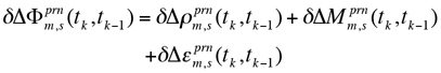
This can be seen in the equation that describes the single-difference multipath between two close-by antennas (one called the “master” and the other the “slave”):

(1)

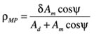
where the angle is the relative multipath phase delay between the antennas and a nearby effective reflector (α₀ is the multipath signal amplitude in the master and slave antennas, and is dependent on the reflector characteristics, reflection coefficient, and receiver tracking loop).

As our study has the objective to mimic as much as possible the multipath effect from effective reflectors in kinematic scenarios with variable dynamics, we decided to name the strategy MIMICS, a slightly contrived abbreviation for “Multipath profile from between receIvers dynaMICS.”

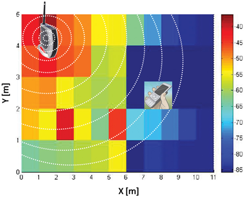
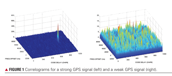
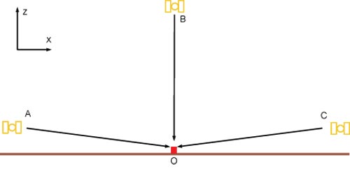
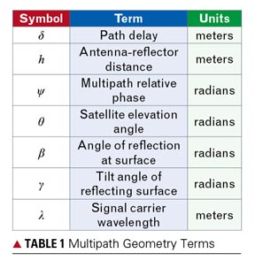
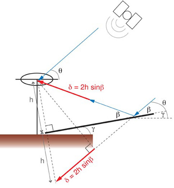
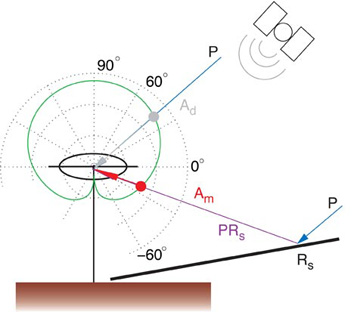
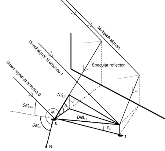
The MIMICS algorithm for a dual-antenna system is based on a specular reflector ray-tracing multipath model (see Figure 1).

Figure 1. 3D ray-tracing modeling of phase multipath for a GNSS dual-antenna system. 0 designates the “master” antenna; 1, the “slave” antenna; Elev and Az, the elevation angle and the azimuth of the satellite, respectively. The other symbols are explained in the text.

After a first step of data synchronization and data-snooping on the data provided by the two receiver antennas, the second step requires the calculation of an approximate position for both antennas, relaxed to a few meters using a standard code solution.

A precise estimation of both antennas’ velocity and acceleration (in real time) is carried out using the carrier-phase observable. Not only should the antenna velocity and acceleration estimates be precisely determined (on the order of a few millimeters per second and a few millimeters per second squared, respectively) but they should also be immune to low-frequency multipath signatures. This is important in our approach, as we use the antennas’ multipath-free dynamic information to separate the multipath in the raw data.

We will start from the basic equations used to derive the single-difference multipath observables.

The observation equation for a single-difference between receivers, using a common external clock (oscillator), is given (in distance units) by:

(2)

where m indicates the master antenna; s, the slave antenna; prn, the satellite number; Δ, the operator for single differencing between receivers; Φ, the carrier-phase observation; ρ, the slant range between the satellite and receiver antennas; N, the carrier-phase ambiguity; M, the multipath; and ε, the system noise.

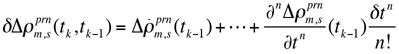
By sequentially differencing Equation (2) in time to remove the single-difference ambiguity from the observation equation, we obtain (as long as there is no loss of lock or cycle slips):

(3)

where

(4)

One of the key ideas in deriving the multipath observable from Equation (3) is to estimate given by Equation (4). We will outline our approach in a later section.

From Equation (3), at the second epoch, for example, we will have:

(5)

If we continue this process up to epoch n, we will obtain an ensemble of differential multipath observations.

If we then take the numerical summation of these, we will have

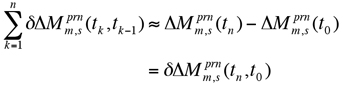(6)

Note that n samples of differential multipath observations are used in Equation (6). Therefore, we need n + 1 observations.

Assume that we perform this process taking n = 1, then n = 2, and so on until we obtain r numerical summations of Equation (6) and then take a second numerical summation of them, we will end up with the following equation:

(7)

where E is the expectation operator.

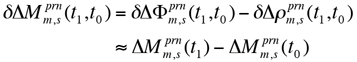
Another key idea in our approach is associated with Equation (7). To isolate the initial epoch multipath, , from the differential multipath observations, the first term on the right-hand side of Equation (7), , should be removed.

This can be accomplished by mechanical calibration and/or numerical randomization. To summarize the idea, we have to create random multipath physically (or numerically) at the initialization step. When the isolation of the initial multipath epoch is completed, we can recover multipath at every epoch using Equation (5).

Digital Differentiators. We introduce digital differentiators in our approach to derive higher order range dynamics (that is, range rate, range-rate change, and so on) using the single-difference (between receivers connected to a common external oscillator) carrier-phase observations. These higher order range dynamics are used in Equation (4).

There are important classes of finite-impulse-response differentiators, which are highly accurate at low to medium frequencies. In central-difference approximations, both the backward and the forward values of the function are used to approximate the current value of the derivative.

Researchers have demonstrated that the coefficients of the maximally linear digital differentiator of order 2N + 1 are the same as the coefficients of the easily computed central-difference approximation of order N.

Another advantage of this class is that within a certain maximum allowable ripple on the amplitude response of the resultant differentiator, its pass band can be dramatically increased. In our approach, this is something fundamental as the multipath in kinematic scenarios is conceptually treated as high-frequency correlated multipath, depending on the platform dynamics and the distance to the reflector(s).

Adaptive Estimation. To derive single-difference multipath at the initial epoch, , a numerical randomization (or mechanical calibration) of the single-difference multipath observations is performed in our approach. A time series of the single-difference multipath observations to be randomized is given as

(8)

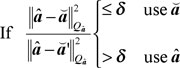
Then our goal is to achieve the following condition:

(9)

It is obvious that the condition will only hold if multipath truly behaves as a stochastic or random process. The estimation of multipath in a kinematic scenario has to be understood as the estimation of time-correlated random errors. However, there is no straightforward way to find the correlation periods and model the errors.

Our idea is to decorrelate the between-antenna relative multipath through the introduction of a pseudorandom motion. As one cannot completely rely only on a decorrelation through the platform calibration motion, one also has to do it through the mathematical “whitening” of the time series.

Nevertheless, the ensemble of data depicted in the above formulation can be modeled as an oscillatory random process, for which second or higher order autoregressive (AR) models can provide more realistic modeling in kinematic scenarios. (An autoregressive process is simply another name for a linear difference equation model where the input or forcing function is white Gaussian noise.) We can estimate the parameters of this model in real time, in a block-by-block analysis using the familiar Yule-Walker equations. A whitening filter can then be formed from the estimation parameters.

We obtain the AR coefficients using the autocorrelation coefficient vector of the random sequences. Since the order of the coefficient estimation depends on the multipath spectra (in turn dependent on the platform dynamics and reflector distance), MIMICS uses a cost function to estimate adaptively, in real time, the appropriate order. An order too low results in a poor whitener of the background colored noise, while an order too large might affect the embedded original signal that we are interested in detecting.

The cost function uses the residual sum of squared error. The order estimate that gives the lowest error is the one chosen, and this task is done iteratively until it reaches a minimum threshold value. Once this stage is fulfilled, the multipath observable can be easily obtained.

Testing

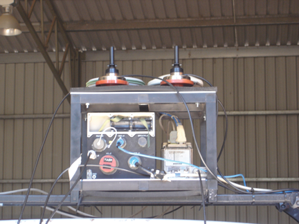
The main test that we have performed so far (using a pair of high performance dual-frequency receivers fed by compact antennas and a rubidium frequency standard, all installed in a vehicle) was designed to evaluate the amount of data necessary to perform the decorrelation, and to determine if the system was observable (in terms of estimating, at every epoch, several multipath parameters from just two-antenna observations). Receiver data was collected and post-processed (so-called RTK-style processing) although, with sufficient computing power, data processing could take place in real, or near real, time.

In a real-life scenario, the platform pseudorandom motions have the advantage that carrier-phase embedded dynamics are typically changing faster and in a three-dimensional manner (antennas sense different pitch and yaw angles). Thus a faster and more robust decorrelation is possible.

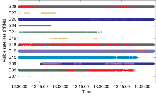
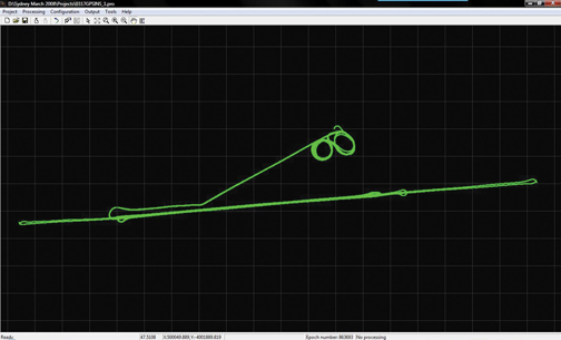
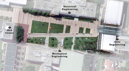
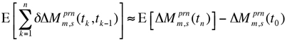
One can see from the bottom picture in Figure 2 the façade of the building behaving as the effective reflector. The vehicle performed several motions, depicted in the bottom panel of Figure 3, always in the visible parking lot, hence the building constantly blocked the view to some satellites. We used only the L1 data from the receivers recorded at a rate of 10 Hz.

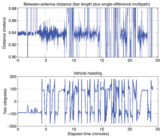
In the bottom panel of Figure 3, one can also see the kind of motion performed by the platform. Accelerations, jerk, idling, and several stops were performed on purpose to see the resultant multipath spectra differences between the antennas. The reference station (using a receiver with capabilities similar to those in the vehicle) was located on a roof-top no more than 110 meters away from the vehicle antennas during the test. As such, most of the usual biases where removed from the solution in the differencing process and the only remaining bias can be attributed to multipath. The data from the reference receiver was only used to obtain the varying baseline with respect to the vehicle master antenna.

In the top panel of Figure 3, one can see the geometric distance calculated from the integer-ambiguity-fixed solutions of both antenna/receiver combinations. Since the distance between the mounting points on the antenna-support bar was accurately measured before the test (84 centimeters), we had an easy way to evaluate the solution quality. The “outliers” seen in the figure come from code solutions because the building mentioned before blocked most of the satellites towards the southeast. As a result, many times fewer than five satellites were available.

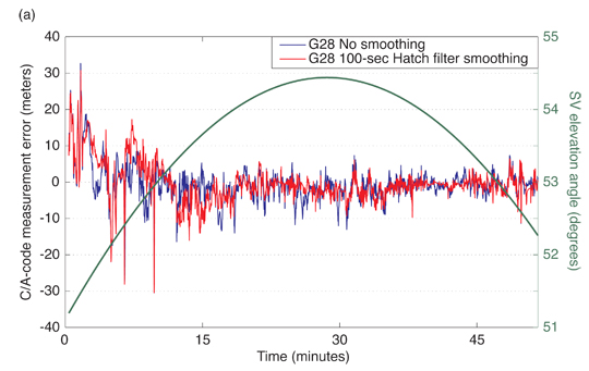
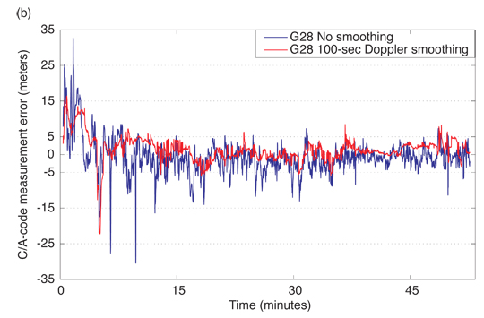
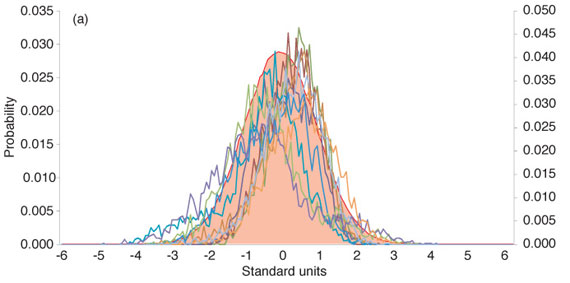
Figure 3. Correlation between vehicle dynamics (heading angle) and the multipath spectra.

Looking at the first nine minutes of results in Figure 4, one can see that when the vehicle is still stationary, the multipath has a very clear quasi-sinusoidal behavior with a period of a few minutes. Also, one can see that it is zero-mean as expected (unlike code multipath). When the vehicle starts moving (at about the four-minute mark), the noise figure is amplified (depending on the platform velocity), but one can still see a mixture of low-frequency components coming from multipath (although with shorter periods).

These results indicate, firstly, that regardless of the distance between two antennas, multipath will not be eliminated after differencing, unlike some other biases. Secondly, when the platform has multiple dynamics, multipath spectra will change accordingly starting from the low-frequency components (due to nearby reflectors) towards the high-frequency ones (including diffraction coming from the building edges and corners). As such, our approach to adaptively model multipath in real time as a quasi-random process makes sense.

Figure 4. Position results from the kinematic test, showing the estimated distance between the two vehicle antennas (upper plot) and the distance between the master antenna and the reference antenna.

Multipath Observables. The multipath observables are obtained through the MIMICS algorithm. It is quite flexible in terms of latency and filter order when it comes to deriving the observables. Basically, it is dependent on the platform dynamics and the amplitude of the residuals of the whitened time series (meaning that if they exceed a certain threshold, then the filtering order doesn’t fit the data).

When comparing the observations delivered every half second for PRN 5 with the ones delivered every second, it is clear that the larger the interval between observations, the better we are able to recover the true biased sinusoidal behavior of multipath. However, in machine control, some applications require a very low latency. Therefore, there must be a compromise between the multipath observable accuracy and the rate at which it is generated.

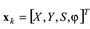
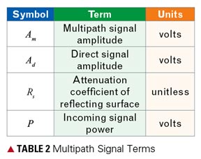
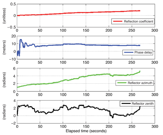
Multipath Parameter Estimation. Once the multipath observables are derived, on a satellite-by-satellite basis, it is possible to estimate the parameters (a₀, the reflection coefficient; γ₀, the phase delay; φ₀, the azimuth of reflected signal; and θ₀, the elevation angle of reflected signal) of the multipath observable described in Equation (1) for each satellite. As mentioned earlier, an EKF is used for the estimation procedure.

When the platform experiences higher dynamics, such as rapid rotations, acceleration is no longer constant and jerk is present. Therefore, a Gauss-Markov model may be more suitable than other stochastic models, such as random walk, and can be implemented through a position-velocity-acceleration dynamic model.

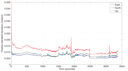
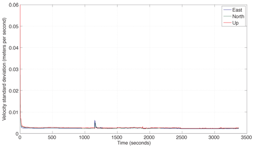
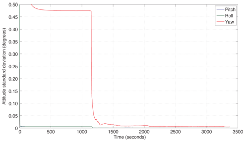
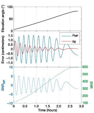
As an example, the results from the multipath parameter estimation are given for satellite PRN 5 in Figure 5. One can see that it takes roughly 40 seconds for the filter to converge. This is especially seen in the phase delay.

Converted to meters, the multipath phase delay gives an approximate value of 10 meters, which is consistent with the distance from the moving platform to the dominant specular reflector (the building’s façade).

Figure 5. PRN 5 multipath parameter estimation.

Multipath Mitigation. After going through all the MIMICS steps,
from the initial data tracking and synchronization between the dual-antenna system up to the multipath parameter estimation for each continuously observed satellite, we can now generate the multipath corrections and thus correct each raw carrier-phase observation.

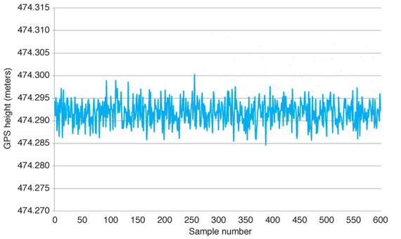
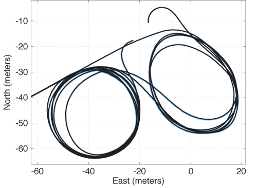
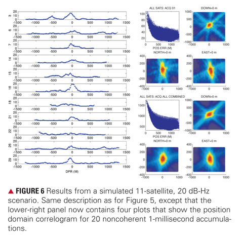
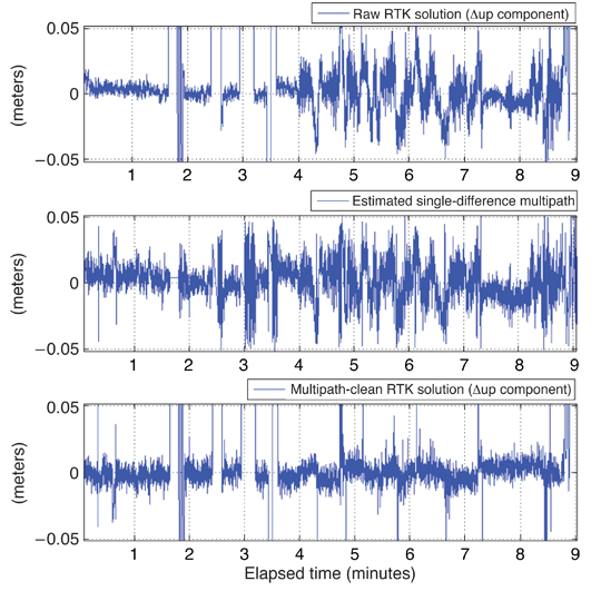
One can see in Figure 6 three different plots from the solution domain depicting the original raw (multipath-contaminated) GPS-RTK baseline up-component (top), the estimated carrier-phase multipath signal (middle), and the difference between the two above time series; that is, the GPS-RTK multipath-ameliorated solution (bottom). A clear improvement is visible. In terms of numbers, and only considering the results “cleaned” from outliers and differential-code solutions (provided by the RTK post-processing software, when carrier-phase ambiguities cannot be fixed), the up-component root-mean-square value before was 2.5 centimeters, and after applying MIMICS it stood at 1.8 centimeters.

Figure 6. MIMICS algorithm results for the vehicle baseline from the first 9 minutes of the test.

Concluding Remarks

Our novel strategy seems to work well in adaptively detecting and estimating multipath profiles in simulated real time (or near real time as there is a small latency to obtain multipath corrections from the MIMICS algorithm). The approach is designed to be applied in specular-rich and varying multipath environments, quite common at construction sites, harbors, airports, and other environments where GNSS-based heading systems are becoming standard. The equipment setup can be simplified, compared to that used in our test, if a single receiver with dual-antenna inputs is employed.

Despite its success, there are some limitations to our approach. From the plots, it’s clear that not all multipath patterns were removed, even though the improvements are notable. Moreover, estimating multipath adaptively in real time can be a problem from a computational point of view when using high update rates. And when the platform is static and no previous calibration exists, the estimation of multipath parameters is impossible as the system is not observable. Nevertheless, the approach shows promise and real-world tests are in the planning stages.

Acknowledgments

The work described in this article was supported by the Natural Sciences and Engineering Research Council of Canada. The article is based on a paper given at the Institute of Electrical and Electronics Engineers / Institute of Navigation Position Location and Navigation Symposium 2010, held in Indian Wells, California, May 6–8, 2010.

Manufacturers

The test of the MIMICS approach used two NovAtel OEM4 receivers in the vehicle each fed by a separate NovAtel GPS-600 “pinweel” antenna on the roof. A Temex Time (now Spectratime) LPFRS-01/5M rubidium frequency standard supplied a common oscillator frequency to both receivers. The reference receiver was a Trimble 5700, fed by a Trimble Zephyr geodetic antenna.

Luis Serrano is a senior navigation engineer at EADS Astrium U.K., in the Ground Segment Group, based in Portsmouth, where he leads studies and research in GNSS high precision applications and GNSS anti-jamming/spoofing software and patents. He is also a completing his Ph.D. degree at the University of New Brunwick (UNB), Fredericton, Canada.

Don Kim is an adjunct professor and a senior research associate in the Department of Geodesy and Geomatics Engineering at UNB where he has been doing research and teaching since 1998. He has a bachelor’s degree in urban engineering and an M.Sc.E. and Ph.D. in geomatics from Seoul National University. Dr. Kim has been involved in GNSS research since 1991 and his research centers on high-precision positioning and navigation sensor technologies for practical solutions in scientific and industrial applications that require real-time processing, high data rates, and high accuracy over long ranges with possible high platform dynamics.

FURTHER READING

• Authors’ Proceedings Paper
“Multipath Adaptive Filtering in GNSS/RTK-Based Machine Automation Applications” by L. Serrano, D. Kim, and R.B. Langley in Proceedings of PLANS 2010, IEEE/ION Position Location and Navigation Symposium, Indian Wells, California, May 4–6, 2010, pp. 60–69, doi: 10.1109/PLANS.2010.5507201.

• Pseudorange and Carrier-Phase Multipath Theory and Amelioration Articles from GPS World
“It’s Not All Bad: Understanding and Using GNSS Multipath” by A. Bilich and K.M. Larson in GPS World, Vol. 20, No. 10, October 2009, pp. 31–39.

“Multipath Mitigation: How Good Can It Get with the New Signals?” by L.R. Weill, in GPS World, Vol. 14, No. 6, June 2003, pp. 106–113.

“GPS Signal Multipath: A Software Simulator” by S.H. Byun, G.A. Hajj, and L.W. Young in GPS World, Vol. 13, No. 7, July 2002, pp. 40–49.

“Conquering Multipath: The GPS Accuracy Battle” by L.R. Weill, in GPS World, Vol. 8, No. 4, April 1997, pp. 59–66.

• Dual Antenna Carrier-phase Multipath Observable
“A New Carrier-Phase Multipath Observable for GPS Real-Time Kinematics Based on Between Receiver Dynamics” by L. Serrano, D. Kim, and R.B. Langley in Proceedings of the 61st Annual Meeting of The Institute of Navigation, Cambridge, Massachusetts, June 27–29, 2005, pp. 1105–1115.

“Mitigation of Static Carrier Phase Multipath Effects Using Multiple Closely-Spaced Antennas” by J.K. Ray, M.E. Cannon, and P. Fenton in Proceedings of ION GPS-98, the 11th International Technical Meeting of the Satellite Division of The Institute of Navigation, Nashville, Tennessee, September 15–18, 1998, pp. 1025–1034.

• Digital Differentiation
“Digital Differentiators Based on Taylor Series” by I.R. Khan and R. Ohba in the Institute of Electronics, Information and Communication Engineers (Japan) Transactions on Fundamentals of Electronics, Communications and Computer Sciences, Vol. E82-A, No. 12, December 1999, pp. 2822–2824.

• Autoregressive Models and the Yule-Walker Equations
Random Signals: Detection, Estimation and Data Analysis by K.S. Shanmugan and A.M. Breipohl, published by Wiley, New York, 1988.

• Kalman Filtering and Dynamic Models
Introduction to Random Signals and Applied Kalman Filtering: with MATLAB Exercises and Solutions, 3rd edition, by R.G. Brown and P.Y.C. Hwang, published by Wiley, New York, 1997.

“The Kalman Filter: Navigation’s Integration Workhorse” by L.J. Levy in GPS World, Vol. 8, No. 9, September 1997, pp. 65–71.

July 1, 2011
Innovation: Doppler-Aided Positioning
Improving Single-Frequency RTK in the Urban Enviornment

By Mojtaba Bahrami and Marek Ziebart

A look at how Doppler measurements can be used to smooth noisy code-based pseudoranges to improve the precision of autonomous positioning as well as to improve the availability of single-frequency real-time kinematic positioning, especially in urban environments.

INNOVATION INSIGHTS by Richard Langley

WHAT DO A GPS RECEIVER, a policeman’s speed gun, a weather radar, and some medical diagnostic equipment have in common? Give up? They all make use of the Doppler effect. First proposed in 1842 by the Austrian mathematician and physicist, Christian Doppler, it is the change in the perceived frequency of a wave when the transmitter and the receiver are in relative motion.

Doppler introduced the concept in an attempt to explain the shift in the color of light from certain binary stars. Three years later, the effect was tested for sound waves by the Dutch scientist Christophorus Buys Ballot. We have all heard the Doppler shift of a train whistle or a siren with their descending tones as the train or emergency vehicle passes us. Doctors use Doppler sonography — also known as Doppler ultrasound — to provide information about the flow of blood and the movement of inner areas of the body with the moving reflectors changing the received ultrasound frequencies. Similarly, some speed guns use the Doppler effect to measure the speed of vehicles or baseballs and Doppler weather radar measures the relative velocity of particles in the air.

The beginning of the space age heralded a new application of the Doppler effect. By measuring the shift in the received frequency of the radio beacon signals transmitted by Sputnik I from a known location, scientists were able to determine the orbit of the satellite. And shortly thereafter, they determined that if the orbit of a satellite was known, then the position of a receiver could be determined from the shift. That realization led to the development of the United States Navy Navigation Satellite System, commonly known as Transit, with the first satellite being launched in 1961. Initially classified, the system was made available to civilians in 1967 and was widely used for navigation and precise positioning until it was shut down in 1996. The Soviet Union developed a similar system called Tsikada and a special military version called Parus. These systems are also assumed to be no longer in use — at least for navigation.

GPS and other global navigation satellite systems use the Doppler shift of the received carrier frequencies to determine the velocity of a moving receiver. Doppler-derived velocity is far more accurate than that obtained by simply differencing two position estimates. But GPS Doppler measurements can be used in other ways, too. In this month’s column, we look at how Doppler measurements can be used to smooth noisy code-based pseudoranges to improve the precision of autonomous positioning as well as to improve the availability of single-frequency real-time kinematic positioning, especially in urban environments.

Correction and Further Details

The first experimental Transit satellite was launched in 1959. A brief summary of subsequent launches follows:
- Transit 1A launched 17 September 1959 failed to reach orbit
- Transit 1B launched 13 April 1960 successfully
- Transit 2A launched 22 June 1960 successfully
- Transit 3A launched 30 November 1960 failed to reach orbit
- Transit 3B launched 22 February 1961 failed to deploy in correct orbit
- Transit 4A launched 29 June 1961 successfully
- Transit 4B launched 15 November 1961 successfully
- Transits 4A and 4B used the 150/400 MHz pair of frequencies and provided geodetically useful results.
- A series of Transit prototype and research satellites was launched between 1962 and 1964 with the first fully operational satellite, Transit 5-BN-2, launched on 5 December 1963.
- The first operational or Oscar-class Transit satellite, NNS O-1, was launched on 6 October 1964.
- The last pair of Transit satellites, NNS O-25 and O-31, was launched on 25 August 1988.
“Innovation” is a regular column that features discussions about recent advances in GPS technology and its applications as well as the fundamentals of GPS positioning. The column is coordinated by Richard Langley of the Department of Geodesy and Geomatics Engineering at the University of New Brunswick, who welcomes your comments and topic ideas. To contact him, email lang @ unb.ca.

Real-time kinematic (RTK) techniques enable centimeter-level, relative positioning. The technology requires expensive, dedicated, dual-frequency, geodetic-quality receivers. However, myriad industrial and engineering applications would benefit from small-size, cost-effective, single-frequency, low-power, and high-accuracy RTK satellite positioning. Can such a sensor be developed and will it deliver? If feasible, such an instrument would find many applications within urban environments — but here the barriers to success are higher. In this article, we show how some of the problems can be overcome.

Single-Frequency RTK

Low-cost single-frequency (L1) GPS receivers have attained mass-market status in the consumer industry. Notwithstanding current levels of maturity in GPS hardware and algorithms, these receivers still suffer from large positioning errors. Any positioning accuracy improvement for mass-market receivers is of great practical importance, especially for many applications demanding small size, cost-effectiveness, low power consumption, and highly accurate GPS positioning and navigation. Examples include mobile mapping technology; machine control; agriculture fertilization and yield monitoring; forestry; utility services; intelligent transportation systems; civil engineering projects; unmanned aerial vehicles; automated continuous monitoring of landslides, avalanches, ground subsidence, and river level; and monitoring deformation of built structures. Moreover, today an ever-increasing number of smartphones and handsets come equipped with a GPS receiver. In those devices, the increasing sophistication of end-user applications and refinement of map databases are continually tightening the accuracy requirements for GPS positioning.

For single-frequency users, the RTK method does appear to offer the promise of highly precise position estimates for stationary and moving receivers and can even be considered a candidate for integration within mobile handhelds. Moreover, the RTK approach is attractive because the potential of the existing national infrastructures such as Great Britain’s Ordnance Survey National GNSS Network-RTK (OSNet) infrastructure, as well as enabling technologies such as the Internet and the cellular networks, can be exploited to deliver RTK corrections and provide high-precision positioning and navigation.

The basic premise of relative (differential) positioning techniques such as RTK is that many of the sources of GNSS measurement errors including the frequency-dependent error (the ionospheric delay) are spatially correlated. By performing relative positioning between receivers, the correlated measurement errors are completely cancelled or greatly reduced, resulting in a significant increase in the positioning accuracy and precision.

Single-Frequency Challenges. Although RTK positioning is a well-established and routine technology, its effective implementation for low-cost, single-frequency L1 receivers poses many serious challenges, especially in difficult and degraded signal environments for GNSS such as urban canyons. The most serious challenge is the use of only the L1 frequency for carrier-phase integer ambiguity resolution and validation. Unfortunately, users with single-frequency capability do not have frequency diversity and many options in forming useful functions and combinations for pseudorange and carrier-phase observables. Moreover, observations from a single-frequency, low-cost receiver are typically “biased” due to the high level of multipath and/or receiver signal-tracking anomalies and also the low-cost patch antenna design that is typically used. In addition, in those receivers, measurements are typically contaminated with high levels of noise due to the low-cost hardware design compared to the high-end receivers. This makes the reliable fixing of the phase ambiguities to their correct integer values, for single-frequency users, a non-trivial problem. As a consequence, the reliability of single-frequency observations to resolve ambiguities on the fly in an operational environ
ment is relatively low compared to the use of dual-frequency observations from geodetic-quality receivers. Improving performance will be difficult, unless high-level noise and multipath can be dealt with effectively or unless ambiguity resolution techniques can be devised that are more robust and are less sensitive to the presence of biases and/or high levels of noise in the observations.

Traditionally, single-frequency RTK positioning requires long uninterrupted initialization times to obtain reliable results, and hence have a time-to-fix ambiguities constraint. Times of 10 to 25 minutes are common. Observations made at tens of continuous epochs are used to determine reliable estimates of the integer phase ambiguities. In addition, these continuous epochs must be free from cycle slips, loss of lock, and interruptions to the carrier-phase signals for enough satellites in view during the ambiguity fixing procedure. Otherwise, the ambiguity resolution will fail to fix the phase ambiguities to correct integer values. To overcome these drawbacks and be able to determine the integer phase ambiguities and thus the precise relative positions, observations made at only one epoch (single-epoch) can be used in resolving the integer phase ambiguities. This allows instantaneous RTK positioning and navigation for single-frequency users such that the problem of cycle slips, discontinuities, and loss of lock is eliminated. However, for single-frequency users, the fixing of the phase ambiguities to their correct integer values using a single epoch of observations is a non-trivial problem; indeed, it is considered the most challenging scenario for ambiguity resolution at the present time.

Instantaneous RTK positioning relies fundamentally upon the inversion of both carrier-phase measurements and code measurements (pseudoranges) and successful instantaneous ambiguity resolution. However, in this approach, the probability of fixing ambiguities to correct integer values is dominated by the relatively imprecise pseudorange measurements. This is more severe in urban areas and difficult environments where the level of noise and multipath on pseudoranges is high. This problem may be overcome partially by carrier smoothing of pseudoranges in the range/measurement domain using, for example, the Hatch filter. While carrier-phase tracking is continuous and free from cycle slips, the carrier smoothing of pseudoranges with an optimal smoothing filter window-width can effectively suppress receiver noise and short-term multipath noise on pseudoranges. However, the effectiveness of the conventional range-domain carrier-smoothing filters is limited in urban areas and difficult GNSS environments because carrier-phase measurements deteriorate easily and substantially due to blockages and foliage and suffer from phase discontinuities, cycle-slip contamination, and other measurement anomalies. This is illustrated in Figure 1. The figure shows that in a kinematic urban environment, frequent carrier-phase outages and anomalies occur, which cause frequent resets of the carrier-smoothing filter and hence carrier smoothing of pseudoranges suffers in robustness and effective continuous smoothing.

Figure 1. Satellite tracking and carrier-phase anomaly summary during the observation time-span. These data were collected in a dense urban environment in both static and kinematic mode. The superimposed red-points show epochs where carrier-phase observables are either missing or contaminated with cycle slips, loss of locks, and/or other measurement anomalies.

Doppler Frequency Shift. While carrier-phase tracking can be discontinuous in the presence of continuous pseudoranges, a receiver generates continuous Doppler-frequency-shift measurements. The Doppler measurements are immune to cycle slips. Moreover, the precision of the Doppler measurements is better than the precision of pseudoranges because the absolute multipath error of the Doppler observable is only a few centimeters. Thus, devising methods that utilize the precision of raw Doppler measurements to reduce the receiver noise and high-frequency multipath on pseudoranges may prove valuable especially in GNSS-challenged environments. Figure 2 shows an example of the availability and the precision of the receiver-generated Doppler measurements alongside the delta-range values derived from the C/A-code pseudoranges and from the L1 carrier-phase measurements. This figure also shows that frequent carrier-phase outages and anomalies occur while for every C/A-code pseudorange measurement there is a corresponding Doppler measurement available.

Figure 2. Plots of C/A-code-pseudorange-derived delta-ranges (top), L1 carrier-phase-derived delta-ranges (middle), and L1 raw receiver-generated Doppler shifts that are transformed into delta-ranges for the satellite PRN G18 during the observation time-span when it was tracked by the receiver (bottom).

Smoothing. A rich body of literature has been published exploring aspects of carrier smoothing of pseudoranges. One factor that has not received sufficient study in the literature is utilization of Doppler measurements to smooth pseudoranges and to investigate the influence of improved pseudorange accuracy on both positioning and the integer-ambiguity resolution. Utilizing the Doppler measurements to smooth pseudoranges could be a good example of an algorithm that maximally utilizes the information redundancy and diversity provided by a GPS/GNSS receiver to improve positioning accuracy. Moreover, utilizing the Doppler measurements does not require any hardware modifications to the receiver. In fact, receivers measure Doppler frequency shifts all the time as a by-product of satellite tracking.

GNSS Doppler Measurement Overview

The Doppler effect is the apparent change in the transmission frequency of the received signal and is experienced whenever there is any relative motion between the emitter and receiver of wave signals. Theoretically, the observed Doppler frequency shift, under Einstein’s Special Theory of Relativity, is approximately equal to the difference between the received and transmitted signal frequencies, which is approximately proportional to the receiver-satellite topocentric range rate.

Beat Frequency. However, the transmitted frequency is replicated locally in a GNSS receiver. Therefore, strictly speaking, the difference of the received frequency and the receiver locally generated replica of the transmitted frequency is the Doppler frequency shift that is also termed the beat frequency. If the receiver oscillator frequency is the same as the satellite oscillator frequency, the beat frequency represents the Doppler frequency shift due to the relative, line-of-sight motion between the satellite and the receiver. However, the receiver internal oscillator is far from being perfect and therefore, the receiver Doppler measurement output is the apparent Doppler frequency shift (that includes local oscillator effects). The Doppler frequency shift is also subject to satellite-oscillator frequency bias and other disturbing effects such as atmospheric effects on the signal propagation.

To estimate the range rate, a receiver typically forms an average of the delta-range by simply integrating the Doppler over a very short period of time (for example, 0.1 second) and then dividing it by the duration of the integration interval. Since the integration of frequency over time gives the phase of the signal over that time interval, the procedure continuously forms the carrier-phase observable that is the integrated Doppler over time. Therefore, Doppler frequency shift can also be estimated by time differencing carrier-phase measurements. The carrier-phase-derived Doppler is com
puted over a longer time span, leading to smoother Doppler measurements, whereas direct loop filter output is an instantaneous measure produced over a short time interval.

Doppler frequency shift is routinely used to determine the satellite or user velocity vector. Apart from velocity determination, it is worth mentioning that Doppler frequency shifts are also exploited for coarse GPS positioning. Moreover, the user velocity vector obtained from the raw Doppler frequency shift can be and has been applied by a number of researchers to instantaneous RTK applications to constrain the float solution and hence improve the integer-ambiguity-resolution success rates in kinematic surveying. In this article, a simple combination procedure of the noisy pseudorange measurements and the receiver-generated Doppler measurements is suggested and its benefits are examined.

Doppler-Smoothing Algorithm Description

Motivated both by the continual availability and the centimeter-level precision of receiver-generated (raw) Doppler measurements, even in urban canyons, a method has been introduced by the authors that utilizes the precision of raw Doppler measurements to reduce the receiver noise and high-frequency multipath on code pseudoranges. For more detail on the Doppler-smoothing technique, see Further Reading. The objective is to smooth the pseudoranges and push the accuracy of the code-based or both code- and carrier-based positioning applications in GNSS-challenged environments.

Previous work on Doppler-aided velocity/position algorithms is mainly in the position domain. In those approaches, the improvement in the quality of positioning is gained mainly by integrating the kinematic velocities and accelerations derived from the Doppler measurement in a loosely coupled extended Kalman filter or its variations such as the complementary Kalman filter. Essentially, these techniques utilize the well-known ability of the Kalman filter to use independent velocity estimates to reduce the noise of positioning solutions and improve positioning accuracy. The main difference among these position-domain filters is that different receiver dynamic models are used.

The proposed method combines centimeter-level precision receiver-generated Doppler measurements with pseudorange measurements in a combined pseudorange measurement that retains the significant information content of each.

Two-Stage Process. The proposed Doppler-smoothing process has two stages: (1) the prediction or initialization stage and (2) the filtering stage. In the prediction stage, a new estimated smoothed value of the pseudorange measurement for the Doppler-smoothing starting epoch is obtained. In this stage, for a fixed number of epochs, a set of estimated pseudoranges for the starting epoch is obtained from the subsequent pseudorange and Doppler measurements. The estimated pseudoranges are then averaged to obtain a good estimated starting point for the smoothing process. The number of epochs used in the prediction stage is the averaging window-width or Doppler-smoothing-filter length. In the filtering stage, the smoothed pseudorange profile is constructed using the estimated smoothed starting pseudorange and the integrated Doppler measurements over time. The Doppler-smoothing procedures outlined here can be performed successively epoch-by-epoch (that is, in a moving filter), where the estimated initial pseudorange (the averaged pseudorange) is updated from epoch to epoch. Alternatively, an efficient and elegant implementation of the measurement-domain Doppler-smoothing method is in terms of a Kalman filter, where it can run as a continuous process in the receiver from the first epoch (or in post-processing software, but then without the real-time advantage). This filter allows real-time operation of the Doppler-smoothing approach.

In the experiments described in this article, a short filter window-width is used. The larger the window width used in the averaging filter process, the more precise the averaged pseudorange becomes. However, this filter is also susceptible to the ionospheric divergence phenomenon because of the opposite signs of the ionospheric contribution in the pseudorange and Doppler observables. Therefore, the ionospheric divergence effect between pseudoranges and Doppler observables increases with averaging window-width and the introduced bias in the averaged pseudoranges become apparent for longer filter lengths.

Using the propagation of variance law, it can be shown that the precision of the delta-range calculated with the integrated Doppler measurements over time depends on both the Doppler-measurement epoch interval and the precision of the Doppler measurements, assuming that noise/errors on the measurements are uncorrelated.

Experimental Results

To validate the improvement in the performance and availability of single-frequency instantaneous RTK in urban areas, the proposed Doppler-aided instantaneous RTK technique has been investigated using actual GPS data collected in both static and kinematic pedestrian trials in central London. In this article, we only focus on the static results and the kinematic trial results are omitted. It is remarked, however, that the data collected in the static mode were post-processed in an epoch-by-epoch approach to simulate RTK processing.

In the static testing, GPS test data were collected with a measurement rate of 1 Hz. At the rover station, a consumer-grade receiver with a patch antenna was used. This is a single-frequency 16-channel receiver that, in addition to the C/A-code pseudoranges, is capable of logging carrier-phase measurements and raw Doppler measurements. Reference station data were obtained from the Ordnance Survey continuously operating GNSS network. Three nearby reference stations were selected that give different baseline lengths: Amersham (AMER) ≈ 38.3 kilometers away, Teddington (TEDD) ≈ 20.8 kilometers away, and Stratford (STRA) ≈ 7.1 kilometers away. In addition, a virtual reference station (VRS) was also generated in the vicinity (60 meters away) of the rover receiver.

Doppler-Smoothing. Before we present the improvement in the performance of instantaneous RTK positioning, the effect of the Doppler-smoothing of the pseudoranges in the measurement domain and comparison with carrier-phase smoothing of pseudoranges is given. To do this, we computed the C/A-code measurement errors or observed range deviations (the differences between the expected and measured pseudoranges) in the static mode (with surveyed known coordinates) using raw, Doppler-smoothed and carrier-smoothed pseudoranges. FIGURE 3a illustrates the effect of 100-second Hatch-filter carrier smoothing and FIGURE 3b shows a 100-second Doppler-smoothing of the pseudoranges for satellite PRN G28 (RINEX satellite designator) with medium-to-high elevation angle. The raw observed pseudorange deviations (in blue) are also given as reference. The quasi-sinusoidal oscillations are characteristic of multipath. Comparing the Doppler-smoothing in Figure 3b to the Hatch carrier-smoothing in Figure 3a, it can be seen that Doppler-smoothing of pseudoranges offers a modest improvement and is more robust and effective than that of the traditional Hatch filter in difficult environments.

Figure 3. Smoothed pseudorange errors (observed range deviations) using the traditional Hatch carrier-smoothing filter. Smoothing filter length in the experiments for both filters was set to 100 seconds. Satellite PRN G28 was chosen to represent a satellite at medium-to-high elevation angle.

Figure 3. Smoothed pseudorange errors (observed range deviations) using the Doppler-smoothing filter. Smoothing filter length in the experiments for both filters was set to 100 seconds. Satellite PRN G28 was chosen to represent a satellite at medium-to-high elevation angle.

Figure 4a illustrates carrier-phase Hatch-filter smoothing for low-elevation angle satellite PRN G18. In this figure, the Hatch carrier-smoothing filter reset is indicated. It can be seen that due to the frequent carrier-phase discontinuities and cycle slips, the smoothing has to be reset and restarted from the beginning and hardly reaches its full potential. In contrast, Doppler smoothing for PRN G18 shown in FIGURE 4b had few filter resets and managed effectively to smooth the very noisy pseudorange in some sections of the data.

Figure 4. Smoothed pseudorange errors (observed range deviations) and filter resets and filter length (window width) using the traditional Hatch carrier-smoothing filter. Smoothing filter length in the experiments for both filters was set to 100 seconds. Satellite PRN G18 was chosen to represent a satellite at low elevation angle as it rises from 10 to 30 degrees.

Figure 4. Smoothed pseudorange errors (observed range deviations) and filter resets and filter length (window width) using the Doppler-smoothing. Smoothing filter length in the experiments for both filters was set to 100 seconds. Satellite PRN G18 was chosen to represent a satellite at low elevation angle as it rises from 10 to 30 degrees.

Considering RTK in this analysis, we can demonstrate the increase in the success rate of the Doppler-aided integer ambiguity resolution (and hence the RTK availability) by comparison of the obtained integer ambiguity vectors from the conventional LAMBDA (Least-squares AMBiguity Decorrelation Adjustment) ambiguity resolution method using Doppler-smoothed pseudoranges with those obtained without Doppler-aiding in post-processed mode. The performance of ambiguity resolution was evaluated based on the number of epochs where the ambiguity validation passed the discrimination/ratio test. The ambiguity validation ratio test was set to the fixed critical threshold of 2.5 in all the experiments. In addition to the ratio test, the fixed solutions obtained using the fixed integer ambiguity vectors that passed the ratio test were compared against the true position of the surveyed point to make sure that indeed the correct set of integer ambiguities were estimated.

The overall performance of the single-epoch single-frequency integer ambiguity resolution obtained by the conventional LAMBDA ambiguity resolution method without Doppler-aiding is shown in Figure 5 for baselines from 60 meters up to 38 kilometers in length. In comparison, the performance of the single-epoch single-frequency integer ambiguity resolution from the LAMBDA method using Doppler-smoothed pseudoranges are shown in Figure 6 for those baselines and they are compared with integer ambiguity resolution success rates of the conventional LAMBDA ambiguity resolution method without Doppler-aiding. Figure 6 shows that using Doppler-smoothed pseudoranges enhances the probability of identifying the correct set of integer ambiguities and hence increases the success rate of the integer ambiguity resolution process in instantaneous RTK, providing higher availability. This is more evident for shorter baselines. For long baselines, the residual of satellite-ephemeris error and atmospheric-delay residuals that do not cancel in double differencing potentially limits the effectiveness of the Doppler-smoothing approach. It is well understood that those residuals for long baselines strongly degrade the performance of ambiguity resolution. Relative kinematic positioning with single frequency mass-market receivers in urban areas using VRS has also shown improvement.

Figure 5. Single-epoch single-frequency integer ambiguity resolution success rate obtained by the conventional LAMBDA ambiguity resolution method without Doppler-aiding.

Figure 6. Plots of integer ambiguity resolution success rates: single-epoch single-frequency integer ambiguity resolution success rate obtained by the conventional LAMBDA ambiguity resolution method without Doppler-aiding (in blue) and using Doppler-smoothed pseudoranges (in green).

Conclusion

In urban areas, the proposed Doppler-smoothing technique is more robust and effective than traditional carrier smoothing of pseudoranges. Static and kinematic trials confirm this technique improves the accuracy of the pseudorange-based absolute and relative positioning in urban areas characteristically by the order of 40 to 50 percent.

Doppler-smoothed pseudoranges are then used to aid the integer ambiguity resolution process to enhance the probability of identifying the correct set of integer ambiguities. This approach shows modest improvement in the ambiguity resolution success rate in instantaneous RTK where the probability of fixing ambiguities to correct integer values is dominated by the relatively imprecise pseudorange measurements.

The importance of resolving the integer ambiguities correctly must be emphasized. Therefore, devising innovative and robust methods to maximize the success rate and hence reliability and availability of single-frequency, single-epoch integer ambiguity resolution in the presence of biased and noisy observations is of great practical importance especially in GNSS-challenged environments.

Acknowledgments

The study reported in this article was funded through a United Kingdom Engineering and Physical Sciences Research Council Engineering Doctorate studentship in collaboration with the Ordnance Survey. M. Bahrami would like to thank his industrial supervisor Chris Phillips from the Ordnance Survey for his continuous encouragement and support. Professor Paul Cross is acknowledged for his valuable comments. The Ordnance Survey is acknowledged for sponsoring the project and providing detailed GIS data.

Manufacturer

The data for the trial discussed in this article were obtained from a u-blox AG AEK-4T receiver with a u-blox ANN-MS-0-005 patch antenna.

Mojtaba Bahrami is a research fellow in the Space Geodesy and Navigation Laboratory (SGNL) at University College London (UCL). He holds an engineering doctorate in space geodesy and navigation from UCL.

Marek Ziebart is a professor of space geodesy at UCL. He is the director of SGNL and vice dean for research in the Faculty of Engineering Sciences at UCL.

FURTHER READING

• Carrier Smoothing of Pseudoranges

“Optimal Hatch Filter with an Adaptive Smoothing Window Width” by B. Park, K. Sohn, and C. Kee in Journal of Navigation, Vol. 61, 2008, pp. 435–454, doi: 10.1017/S0373463308004694.

“Optimal Recursive Least-Squares Filtering of GPS Pseudorange Measurements” by A. Q. Le and P. J. G. Teunissen in VI Hotine-Marussi Symposium on Theoretical and Computational Geodesy, Wuhan, China, May 29 – June 2, 2006, Vol. 132 of the International Association of Geodesy Symposia, Springer-Verlag, Berlin and Heidelberg, 2008, Part II, pp. 166–172, doi: 10.1007/978-3-540-74584-6_26.

“The Synergism of GPS Code and Carrier Measurements” by R. Hatch in Proceedings of the 3rdInternational Geodetic Symposium on Satellite Doppler Positioning, Las Cruces, New Mexico, February 8-12, 1982, Vol. 2, pp. 1213–1231.

• Combining Pseudoranges and Carrier-phase Measurements in the Position Domain

“Position Domain Filtering and Range Domain Filtering for Carrier-smoothed-code DGNSS: An Analytical Comparison” by H. Lee, C. Rizos, and G.-I. Jee in IEE Proceedings Radar, Sonar and Navigation, Vol. 152, No. 4, August 2005, pp. 271–276, doi:10.1049/ip-rsn:20059008.

“Complementary Kalman Filter for Smoothing GPS Position with GPS Velocity” by H. Leppakoski, J. Syrjarinne, and J. Takala in Proceedings of ION GPS/GNSS 2003, the 16th International Technical Meeting of the Satellite Division of The Institute of Navigation, Portland, Oregon, September 9–
12, 2003, pp. 1201–1210.

“Precise Platform Positioning with a Single GPS Receiver” by S. B. Bisnath, T. Beran, and R. B. Langley in GPS World, Vol. 13, No. 4, April 2002, pp. 42–49.

“GPS Navigation: Combining Pseudorange with Continuous Carrier Phase Using a Kalman Filter” by P. Y. C. Hwang and R. G. Brown in Navigation, Journal of The Institute of Navigation, Vol. 37, No. 2, 1990, pp. 181–196.

• Doppler-derived Velocity Information and RTK Positioning

“Advantage of Velocity Measurements on Instantaneous RTK Positioning” by N. Kubo in GPS Solutions, Vol. 13, No. 4, 2009, pp. 271–280, doi: 10.1007/s10291-009-0120-9.

• Doppler Smoothing of Pseudoranges and RTK Positioning

Doppler-Aided Single-Frequency Real-Time Kinematic Satellite Positioning in the Urban Environment by M. Bahrami, Ph.D. dissertation, Space Geodesy and Navigation Laboratory, University College London, U.K., 2011.

“Instantaneous Doppler-Aided RTK Positioning with Single Frequency Receivers” by M. Bahrami and M. Ziebart in Proceedings of PLANS 2010, IEEE/ION Position Location and Navigation Symposium, Indian Wells, California, May 4–6, 2010, pp. 70–78, doi: 10.1109/PLANS.2010.5507202.

“Getting Back on the Sidewalk: Doppler-Aided Autonomous Positioning with Single-Frequency Mass Market Receivers in Urban Areas” by M. Bahrami in Proceedings of ION GNSS 2009, the 22nd International Technical Meeting of the Satellite Division of The Institute of Navigation, Savannah, Georgia, 22–25 September 2009, pp. 1716–1725.

• Integer Ambiguity Resolution

“GPS Ambiguity Resolution and Validation: Methodologies, Trends and Issues” by D. Kim and R. B. Langley in Proceedings of the 7th GNSS Workshop – International Symposium on GPS/GNSS, Seoul, Korea, 30 November – 2 December 2000, Tutorial/Domestic Session, pp. 213–221.

The LAMBDA Method for Integer Ambiguity Estimation: Implementation Aspects by P. de Jong and C. Tiberius. Publications of the Delft Geodetic Computing Centre, No. 12, Delft University of Technology, Delft, The Netherlands, August 1996.

“A New Way to Fix Carrier-phase Ambiguities” by P.J.G. Teunissen, P.J. de Jonge, and C.C.J.M. Tiberius in GPS World, Vol. 6, No. 4, April 1995, pp. 58–61.

“The Least-Squares Ambiguity Decorrelation Adjustment: a Method for Fast GPS Integer Ambiguity Estimation” by P.J.G. Teunissen in Journal of Geodesy, Vol. 70, No. 1–2, 1995, pp. 65–82, doi: 10.1007/BF00863419.
May 1, 2011
Innovation: Accuracy versus Precision

A Primer on GPS Truth

By David Rutledge

True to its word origins, accuracy demands careful and thoughtful work. This article provides a close look at the differences between the precision and accuracy of GPS-determined positions, and should alleviate the confusion between the terms — making abuse of the truth perhaps less likely in the business of GPS positioning.

INNOVATION INSIGHTS by Richard Langley

JACQUES-BÉNIGNE BOSSUET, the 17th century French bishop and pulpit orator, once said “Every error is truth abused.” He was referring to man’s foibles, of course, but this statement is much more general and equally well applies to measurements of all kinds. As I am fond of telling the students in my introduction to adjustment calculus course, there is no such thing as a perfect measurement. All measurements contain errors. To extract the most useful amount of information from the measurements, the errors must be properly analyzed.

Errors can be broadly grouped into two major categories: biases, which are systematic and which can be modeled in an equation describing the measurements, thereby removing or significantly reducing their effect; and noise or random error, each value of which cannot be modeled but whose statistical properties can be used to optimize the analysis results.

Take GPS carrier-phase measurements, for example. It is a standard approach to collect measurements at a reference station and a target station and to form the double differences of the measurements between pairs of satellites and the pair of receivers. By so doing, the biases in the modeled measurements that are common to both receivers, such as residual satellite clock error, are canceled or significantly reduced. However, the random error in the measurements due to receiver thermal noise and the quasi-random effect of multipath cannot be differenced away. If we estimate the coordinates of the target receiver at each epoch of the measurements, how far will they be from the true coordinates?

That depends on how well the biases were removed and the effects of random error. By comparing the results from many epochs of data, we might see that the coordinate values agree amongst themselves quite closely; they have high precision. But, due to some remaining bias, they are offset from the true value; their accuracy is low. Two different but complementary measures for assessing the quality of the results.

In this month’s column, we will examine the differences between the precision and accuracy of GPS-determined positions and, armed with a better understanding of these often confused terms, perhaps be less likely to abuse the truth in the business of GPS positioning.

“Innovation” features discussions about advances in GPS technology, its applications, and the fundamentals of GPS positioning. The column is coordinated by Richard Langley, Department of Geodesy and Geomatics Engineering, University of New Brunswick.

For many, Global Positioning System (GPS) measurement errors are a mystery. The standard literature rarely does justice to the complexity of the subject. A basic premise of this article is that despite this, most practical techniques to evaluate differential GPS measurement errors can be learned without great difficulty, and without the use of advanced mathematics. Modern statistics, a basic signal-processing framework, and the careful use of language allow these disruptive errors to be easily measured, categorized, and discussed.

The tools that we use today were developed over the last 350 years as mathematicians struggled to combine measurements and to quantify error, and to generally understand the natural patterns. A distinguished group of scientists carried out this work, including Adrien-Marie Legendre, Abraham de Moivre, and Carl Friedrich Gauss. These luminaries developed potent techniques to answer numerous and difficult questions about measurements.

We use two special terms to describe systems and methods that measure or estimate error. These terms are precision and accuracy. They are terms used to describe the relationship between measurements, and to underlying truth. Unfortunately, these two terms are often used loosely (or worse used interchangeably), in spite of their specific definitions. Adding to the confusion, accuracy is only properly understood when divided into its two natural components: internal accuracy and external accuracy.

GPS measurements are like many other signals in that with enough samples the probability distribution for each of the three components is typically bell-shaped, allowing us to use a particularly powerful error model. This bell-shaped distribution is often called a Gaussian distribution (after Carl Friedrich Gauss, the great German mathematician) or a normal distribution. Once enough GPS signal is accumulated, a normal distribution forms. Then, potent tools like Gauss’s normal curve error model and the associated square-root law can be brought to bear to estimate the measurement error.

An interesting aspect of GPS, however, is that over short periods of time, data are not normally distributed. This is of great importance because many applications are based upon small datasets. This results in a fundamental division in terms of how measurement error is evaluated. For short periods of time, the gain from averaging is difficult to quantify, and it may or may not improve accuracy. For longer periods of time the gain from averaging is significant, a normal distribution forms, and the square-root law is used to estimate the gain. The absence of a Gaussian distribution in these datasets (1 hour or less) is one source of the confusion surrounding measurement error. Another source of confusion is the richly nuanced concept of accuracy. By closely looking at each of these, a clear picture emerges about how to effectively analyze and describe differential GPS measurement error.

The GPS Signal

It is helpful to consider consecutive differential GPS measurements as a signal, and thus from the vantage of signal processing. Here, we use the term measurement to refer to position solutions rather than the raw carrier-phase and pseudorange measurements a receiver makes. Sequential position measurements from a GPS system are discrete signals, the result of quantization, transformation, and other processing of the code and carrier data into more meaningful digital output. In comparison, a continuous signal is usually analog based and assumes a continuous range of values, like a DC voltage. A signal is a way of describing how one value is related to another.

Figure 1 shows a time series consisting of a discrete signal from a typical GPS dataset (height component). These data are based on processing carrier-phase data from a pair of GPS receivers, in double-difference mode, holding the position of one fixed while estimating that of the other. The vertical axis is often called the dependent variable and can be assigned many labels. Here it is labeled GPS height. The horizontal axis is typically called the independent variable, or the domain. This axis could be labeled either time or sample number, depending on how we want this variable to be represented. Here it is labeled sample number. The data in Figure 1 are in the time domain because each GPS measurement was sampled at equal intervals of time (1 second). We’ll refer to a particular data value (height) as x_i.

Figure 1. A 10-minute sample of GPS height data.

Ten minutes of GPS data are displayed in Figure 1. These data are the first 600 measurements from a larger 96-hour dataset that forms the basis of this paper. The mean (or average) is the first number to calculate in any error-assessment work. The mean is indicated by . There is nothing fancy in computing the mean; simply add all of the measurements together and divide by the total sample number, or N. Equation 1 is its mathematical form:

[1]

The mean for these data is 474.2927 meters, and gives us the average value or “center” of the signal. By itself, the mean provides no information on the overall measurement error, so we start our investigation by calculating how far each GPS height determination is located away from the mean, or how the measurements spread or disperse away from the center. In mathematical form, the expression denotes how far the ith sample differs from the mean.

As an example, the first sample deviates by 0.0038 meters (note that we always take the absolute value). The average deviation (or average error) is found by simply summing the deviations of all of the samples and dividing by N. The average deviation quantifies the spreading of the data away from the mean, and is a way of calculating precision. When the average deviation is small, we say the data are precise. For these data, the average deviation is 0.0044 meters.

For most GPS error studies, however, the average deviation is not used. Instead, we use the standard deviation where the averaging is done with power rather than amplitude. Each deviation from the mean, , is squared, , before taking the average. Then the square root is taken to adjust for the initial squaring. Equation 2 is the mathematical form of the standard deviation (SD):

[2]

The standard deviation for the data in Figure 1 is 0.0052 meters.

But note that these data have a changing mean (as indicated by the slowly varying trend). The statistical or random noise remains fairly constant, while the mean varies with time. Signals that change in this manner are called nonstationary. In this 10-minute dataset, the changing mean interferes with the calculation of the standard deviation. The standard deviation of this dataset is inflated to 0.0052 meters by the shifting mean, whereas if we broke the signal into one-minute pieces to compensate, it would be only 0.0026 meters.

To highlight this, Figure 2 is presented as an artificially created (or synthetic) dataset with a stationary mean equal to the first data point in Figure 1, and with the standard deviation set to 0.0026 meters. This figure, with its stable mean and consistent random noise, displays a Gaussian distribution (as we will soon see graphically), and illustrates what our dataset is not.

Figure 2. A 10-minute sample of synthetic data.

Contrasting these two datasets helps us to understand a critical aspect of differential GPS data. Analyzing a one-minute segment of GPS data from Figure 1 would provide a correct estimate of the standard deviation of the higher frequency random component, but would likely provide an incorrect estimate of the mean. This is because of its wandering nature; a priori we do not know which of the 10 one-minute segments is closer to the truth. It is tempting then to think that by calculating the statistics on the full 10 minutes we will conclusively have a better estimate of the mean, but this is not true.

The mean might be moving toward or away from truth over the time period. It is not yet centered over any one value because its distribution is not Gaussian. What’s more, when we calculate the statistics on the full 10 minutes of data, we will distort the standard deviation of the higher frequency random component upwards (from 0.0026 meters to 0.0052 meters).

This situation results in a great deal of confusion with respect to the study of GPS measurement error. When we look at Figures 1 and 2 side by side we see the complication. Figure 2 is a straightforward signal with stationary mean and Gaussian noise. Averaging a consecutive series of data points will improve the accuracy. Figure 1 is composed of a higher frequency random component (shown by the circle), plus a lower frequency non-random component. It is the superimposition of these two that causes the trouble. We cannot reliably calculate the increase in accuracy as we accumulate more data until the non-random component converges to a random process. This results in a very interesting situation; in numerous cases gathering more data can actually move the location parameter (the mean, ) away from truth rather than toward it.

To fully understand the implications of this, consider its effect on estimating accuracy. If the mean is stationary, statistical methods developed by Gauss and others could be used to estimate the measurement error of an average for any set of N samples. For example, the so-called standard error of the average (SE) can be computed by taking the square root of the sample number, multiplying it by the standard deviation, and then dividing by the sample number (a method to provide an estimate of the error for any average that is randomly distributed). Equation 3 is its mathematical form:

[3]

which simplifies to S/√N . This model can only be used if the data have a Gaussian distribution. Clearly this model cannot be used for the data in Figure 1, but can be used for the data in Figure 2. The implications are significant. The data from Figure 1 are not Gaussian because of the nonstationary mean, so we do not know if the gain from 10 minutes of averaging is better or worse than the first measurement. By contrast, the data in Figure 2 are Gaussian, so we know that the average of the series is more accurate than any individual measurement by a factor equal to the square root of the measurements.

By shifting these data into another domain we can see this more clearly. Figure 3 shows the 10 minutes of GPS data from Figure 1 plotted as a histogram or distribution of the number of data values falling within particular ranges of values. We call each range a bin. The histogram shows the frequencies with which given ranges of values occur. Hence it is also known as a frequency distribution. The frequency distribution can be converted to a probability distribution by dividing the bin totals by the total number of data values to give the relative frequency. If the number of observations is increased indefinitely and simultaneously the bin size is made smaller and smaller, the histogram will tend to a smooth continuous curve called a probability distribution or, more technically, a probability density function. A normal probability distribution curve is overlain in Figure 3 for perspective. This curve simultaneously demonstrates what a normal distribution looks like, and serves to graphically display the underlying truth (by showing the correct frequency distribution, mean, and standard deviation). It was generated by calculating the statistics of the 96-hour dataset, then using a random-number generator with adjustable mean and standard deviation (this is an example of internal accuracy, and will be discussed at length in an upcoming section). We can see that our Figure 1 dataset is not Gaussian because it does not have a credible bell shape. By contrast, when we convert the synthetic data from Figure 2 into a frequency distribution, we see the effect of the stationary mean — the data are distributed in a normal fashion because the mean is not wandering.

Figure 3. Frequency distribution of a 10-minute sample of GPS height data.

Recall that all that is needed to use the Gauss model of measurement error is the presence of a random process. Mathematically, the measurement accuracy for the average of the data in Figures 1 and 3 is the overall standard deviation, or 0.0052 meters, because there is no gain per the square-root law. In comparison, the measurement accuracy for the average in Figure 4 is SE = (√ 600•0.0026) / 600 = 0.0001 meters. The standard deviation from the mean is still 0.0026 meters, but the accuracy of the averaged 600 samples is 0.0001 meters. Recall that precision is the spreading away from the mean, whereas accuracy is closeness to truth. When a process is normally distributed, the more data we collect the closer we come to underlying truth. The difference between the two is remarkable. Measurement error can be quickly beaten down when the frequency distribution is normal. This has significant implications for people who collect more than an hour of data, and raises the following question: At what point can we use the standard error model?

Figure 4. Frequency distribution of a 10-minute sample of synthetic data.

Frequency Distribution

In an ideal world, GPS data would display a Gaussian distribution over both short and long time intervals. This is not the case because of the combination of frequencies that we saw earlier (random + non-random). As an aside, this combination is a good example of why power is used rather than amplitude to calculate the deviation from the mean. When two signals combine, the resultant noise is equal to the combined power, and not amplitude.

Interesting things happen as we accumulate more data and continue our analysis of the 96-hour dataset. Earlier we discussed calculating the SD and the mean, and we looked at short intervals of GPS data in the time domain and the frequency-distribution domain. Moving forward, we will continue to look at the data in the frequency-distribution domain because it is far easier to recognize a Gaussian distribution there. The goal is to discover the approximate point at which GPS data behave in a Gaussian fashion as revealed by the appearance of a true bell curve distribution.

Figure 5 shows one minute of GPS data along with the “truth” curve for perspective. This normal curve, as discussed above, was generated using a random number generator with programmable SD and mean variables. The left axis shows the probability distribution for the GPS data, and the right axis shows the probability distribution function for the normal curve. This figure reinforces what we already know: one minute of GPS data are typically not Gaussian (Figure 3 shows the same thing for 10 minutes of data).

Figure 5. Frequency distribution of a 1-minute sample of GPS height data.

Figure 6 shows 1 hour of GPS data. The data in Figure 6 show the beginnings of a clear normal distribution. Note that the mean of the GPS data is still shifted from the mean of the overall dataset. The appearance of a normal distribution at around 1 hour of data indicates that we can begin use of the standard error model, or the Gaussian error model. Recall that this states that the average of the collection of measurements is more accurate that any individual measurement by a factor equal to the square root of the number of measurements, provided the data follow the Gauss model and are normally distributed. For one hour of data, the gain is square root of 1 times the SD divided by N. In effect, no gain. But from this point forward each hour of data provides √N gain. Figure 7 shows 12 hours of data with a gain of √12. By calculating the standard error for the average of 12 hours of data, SE = (√12•0.0069)/12, or 0.0020 meters, we see a clear gain in accuracy. Notice also that at 12 hours the normal curve and the GPS data are close to being one and the same.

Figure 6. Frequency distribution of a 1-hour sample of GPS height data.

Figure 7. Frequency distribution of a 12-hour sample of GPS height data.

Several things are worth pointing out here. The non-stationary mean converts to a Gaussian process after approximately 1 hour. There is nothing magical about this; conversion at some point is a necessary condition for the system to successfully operate. If it did not, the continually wandering mean would render it of little use as a commercial positioning system. Because it is non-stationary over the shorter occupations considered normal for many applications, it is confusing. Collecting more data in some instances can contribute to less accuracy. This situation also creates a gulf between those who collect an hour or two, and those who collect continuously. It is worth emphasizing that the distribution of data under our “truth” curve fills out nicely after 12 hours. This coincides with one pass of the GPS constellation, suggesting (as we already know) that a significant fraction of the wandering mean is affected by the geometrical error between the observer and the space vehicles overhead.

By looking at the 12 one-hour Gaussian distributions that comprise a 12-hour dataset, we see clearly what Francis Galton discovered in the 1800s. A normal mixture of normal distributions is itself normal, as Figure 8 shows. This sounds simple, but in fact it has significant implications. The unity between consecutive 1-hour segments of our dataset is the normal outline, reinforcing the increasing accuracy of the location parameter, , as more and more normal curves are summed together.

Figure 8. (a) Frequency distribution of 12 1-hour samples of GPS height data; (b) the 12 1-hour samples combined.

Internal vs. External Accuracy

Figure 9 shows the relationship between precision and accuracy. The dashed vertical line indicates the mean of the dataset (the inflection point at which the histogram balances). The red arrows bracket the spread of the dataset at 1 standard deviation from the mean (precision), while the black arrows bracket the offset of the mean from truth (accuracy). Notice that the mean ( ) is a location parameter, while the standard deviation (<e
m>s) is a spread parameter. What we do with the mean is accuracy related; what we do with the standard deviation is precision related.

Figure 9. Relationship between precision and accuracy.

Accuracy is the difference between the true value and our best estimate of it. While the definition may be clear, the practice is not. Earlier we discussed two techniques used to calculate precision — the average deviation, and the standard deviation. We also discussed the square-root law that estimates the measurement error of a series of random measurements. As we saw, it was not possible to calculate this until roughly 1 hour of data had been collected. Furthermore, the data were said to be accurate when a good correlation appeared between the overlain curve and the GPS data at 12 hours.

But here is the interesting thing; the truth curve was derived internally. As previously discussed, data were accumulated for 96 hours, and then statistics were calculated on the overall dataset. Then a random number generator with programmable mean and standard deviation was used to generate a perfectly random distribution curve with the same location parameter and spread. This was declared as truth, and then smaller subsets of the same dataset were essentially compared with a perfect version of itself! This is an example of what is called internal accuracy.

By contrast, external accuracy is when a standard, another instrument, or some other reference system is brought to bear to gauge accuracy. A simple example is when a physical standard is used to confirm a length measurement. For instance, a laser measurement of 1 meter might be checked or calibrated against a 1-meter platinum iridium bar that is accepted as a standard. The important point here is that truth does not just appear — it has to be established through an internal or external process.

Accuracy can be evaluated in two ways: by using information internal to the data, and by using information external to the data. The historical development of measurement error is mostly about internal accuracy. Suppose that a set of astronomical measurements is subjected to mathematical analysis, without explicit reference to underlying truth. This is internal accuracy, and was famously expressed by Isaac Newton in Book Three of his Principia: “For all of this it is plain that these observations agree with theory, so far as they agree with one another.”

Internal accuracy constrains and simplifies the problem. It eliminates the need to bring other instruments or systems to bear. It makes the problem manageable by allowing us to use what we already have. Most importantly, it eliminates the need to consider point of view. Because we are not venturing outside of the dataset, it becomes the reference frame. By contrast, when you ponder bringing an external source of accuracy to bear it gets complicated, especially with GPS.

For example, is it sufficient to use one GPS receiver to check the accuracy of another, or should an entirely different instrument be used? Is it suitable to use the Earth-centered, Earth-fixed GPS frame to check itself, or should another frame be used? If we use another frame, should it extend beyond the Earth, or is it sufficient to consider accuracy from an Earth perspective? When we say a GPS measurement is accurate, what we are really saying is that it is accurate with respect to our reference frame. But what if you were an observer located on the Sun? An Earth-centric frame no longer makes sense when the point that you wish to measure is located on a planet that is rotating in an orbit around you. For an observer on the Sun, a Sun-centered, Sun-fixed reference frame would probably make more sense, and would result in easier to understand measurements. But we are not on the Sun, so a reference frame that rotates with the Earth — making fixed points appear static — makes the most sense. The difference between the two is that of perspective, and it can color our perception of accuracy.

Internal accuracy assessments sidestep these complications, but make it difficult to detect systematic errors or biases. Keep in mind that any given GPS measurement can be represented by the following equation: measurement = exact value + bias + random error. The random-error component presents roughly the same problem for both internal and external assessments. The bias however, requires external truth for detection. There is no easy way to detect a constant shift from truth in a dataset by studying only the shifted dataset.

In practice, people generally look for internal consistency, as Newton did. We look for consistency within a continuous dataset, or we collect multiple datasets at different times and then look for consistency between datasets. It is not uncommon to use the method taken in this article: let data accumulate until one is confident that the mean has revealed truth, and then use this for all further analysis. For this approach, accuracy implies how the measurements mathematically “agree with one another.”

All of this shows that accuracy is a very malleable term. Internal accuracy assumes that the process is centered over truth. It is implicitly understood that more measurements will increase the accuracy once the distribution is normal. The standard error is calculated by taking the square root of the sample number, multiplying it by the standard deviation, and then dividing by the sample number. With more samples, the standard error of the average decreases, and we say that the accuracy is increasing. Internal accuracy is a function of the standard deviation and the frequency distribution.

External accuracy derives truth from a source outside the dataset. Accuracy is the offset between this truth and the measurement, and not a function of the standard deviation of the dataset. The concept is simple, but in practice establishing an external standard for GPS can be quite challenging. For counterpoint, consider the convenient relationship between a carpenter and a tape measure. He is in the privileged position of carrying a replica of the truth standard. GPS users have no such tool. It is impossible to bring a surrogate of the GPS system to bear to check a measurement. Fortunately, new global navigation satellite systems are coming on line to help, but a formal analysis of how to externally check GPS accuracy leads one into a morass of difficult questions.

Accuracy is not a fundamental characteristic of a dataset like precision. This is why accuracy lacks a formal mathematical symbol. One needs to look no further than internal accuracy for the proof. For a dataset that is shifted away from truth, or biased, no amount of averaging will improve its accuracy. Because it is possible to be unaware of a bias using internal accuracy assessments, it follows that accuracy cannot be inherent to a dataset.

Looking at the interplay between mathematical notation and language provides more insight. For example, we describe the mathematical symbol with the word mean. We don’t stop there, however; we also sometimes call it the average. Likewise, the mathematical symbol s is described by the words standard deviation, but we also know s as precision, sigma, repeatability, and sometimes spread. English has a wealth of synonyms, giving it an ability to describe that is unparalleled. In fact, it is one of only a few languages that require a thesaurus. This is why it is important to make a clear distinction between the relatively clear world of mathematical notation and the more free-form world of words. Language gives us flexibility and power, but can also confound with its ability to provide subtle differences in meaning.

When we look at the etymology of the word accuracy, we can see that it is aptly named. It comes from the Latin word accuro, which means to take care of, to prepare with care, to trouble about, and to do painstakingly. Accuro is itself derived from the root cura, which means roughly the same thing and is familiar to us today in the form of the word curator. It is fitting language for a process that requires so much care.

When we discuss measurement error we seldom use mathematical symbols; we use language that is every bit as important as the symbols. The word error itself derives from the Latin erro, which means to wander, or to stray, and suitably describes the random tendency of measurements.

Whether we describe it with mathematics or language, error describes a fundamental pattern we see in nature; independent measurements tend to randomly wander around a mean. When the frequency distribution is normal, accuracy from the underlying truth occurs in multiples of √N. Error is the umbrella covering the other terms because it is the natural starting point for any discussion. Because of this, precision and accuracy are naturally subsumed under error, with accuracy further split into internal and external accuracy. By contemplating all of this, we expose the healthy tension between words and mathematical notation. Neither is perfect. Mathematics establishes natural patterns and provides excellent approximation tools, but is not readily available to everyone. Language opens the door to perspective and point of view, and invites questions in a way that mathematical notation does not.

Final Notes

Making sense of GPS error requires that we take a close look at the intricacies of the GPS signal, with particular attention to the ramp up to a normal distribution. It also requires a good hard look at the language of error. Shifting the GPS data back and forth between the frequency-distribution and time domains nicely illustrates the complications imposed by a non-stationary mean. Datasets that are an hour or less in duration do not always increase in accuracy when the measurements are averaged. Averaging may provide a gain, but it is not a certainty. When the non-stationary mean converges to a Gaussian process after an hour or so, we begin to see what De Moivre discovered almost 275 hundred years ago: accuracy increases as the square root of the sample size.

The GPS system is so good that the division of accuracy into its proper internal and external accuracy components is shimmering beneath the surface for most users. It is rare that a set of GPS measurements has a persistent bias, so internal accuracy assessments are usually appropriate. This should not stop us from being careful with how we discuss accuracy, however. Some attempt should be made to distinguish between the two types, and neither should be used interchangeably with precision. What’s more, while accuracy is not something intrinsic to a dataset like precision, it is still much more than just a descriptive word. Accuracy is the hinge between the formal world of mathematics and point of view. Its derivation from N and s in internal assessments stands in stark contrast to the more perspective-driven derivation often found in external assessments. When carrying out internal assessments, we must be aware that we are assuming that the measurements are centered over truth. When carrying out external assessments, we must be mindful of what outside mechanism we are using to provide truth. True to its word origins, accuracy demands careful and thoughtful work.

David Rutledge is the director for infrastructure monitoring at Leica Geosystems in the Americas. He has been involved in the GPS industry since 1995, and has overseen numerous high-accuracy GPS projects around the world.

FURTHER READING

• Highly Readable Texts on Basic Statistics and Probability
The Drunkard’s Walk: How Randomness Rules Our Lives by L. Mlodinow, Pantheon Books, New York, 2008.

Noise by B. Kosko,Viking Penguin, New York, 2006.

• Basic Texts on Statistics and Probability Theory
A Practical Guide to Data Analysis for Physical Science Students by Louis Lyons, Cambridge University Press, Cambridge, U.K., 1991.

Principles of Statistics by M.G. Bulmer, Dover Publications, Inc., New York, 1979.

• Relevant GPS World Articles
“Stochastic Models for GPS Positioning: An Empirical Approach” by R.F. Leandro and M.C. Santos in GPS World, Vol. 18, No. 2, February 2007, pp. 50–56.

“GNSS Accuracy: Lies, Damn Lies, and Statistics” by F. van Diggelen in GPS World, Vol. 18, No. 1, January 2007, pp. 26–32.

“Dam Stability: Assessing the Performance of a GPS Monitoring System” by D.R. Rutledge, S.Z. Meyerholtz, N.E. Brown, and C.S. Baldwin in GPS World, Vol. 17, No. 10, October 2006, pp. 26–33.

“Standard Positioning Service: Handheld GPS Receiver Accuracy” by C. Tiberius in GPS World, Vol. 14, No. 2, February 2003, pp. 44–51.

“The Stochastics of GPS Observables” by C. Tiberius, N. Jonkman, and F. Kenselaar in GPS World, Vol. 10, No. 2, February 1999, pp. 49–54.

“The GPS Observables” by R.B. Langley in GPS World, Vol. 4, No 4, April 1993, pp. 52–59.

“The Mathematics of GPS” by R.B. Langley in GPS World, Vol. 2, No. 7, July/August 1991, pp. 45–50.

May 1, 2010
Innovation: Hybrid Positioning

A Prototype System for Navigation in GPS-Challenged Environments

By Chris Rizos, Dorota A. Grejner-Brzezinska, Charles K. Toth, Andrew G. Dempster, Yong Li, Nonie Politi, Joel Barnes, Hongxing Sun, and Leilei Li

A team of Australian and U.S. researchers have integrated a ground-based system with GPS and INS to create a hybrid system that provides precise and accurate position information continuously in a variety of environments where GPS alone comes up short.

INNOVATION INSIGHTS by Richard Langley

GPS HAS ITS LIMITATIONS. Although it is a 24/7 global system, it doesn’t work everywhere. The microwave radio signals transmitted by the satellites are rather weak, and although they can provide excellent positioning performance when a receiver’s antenna has a direct line-of-sight view of a sufficient number of satellites well spread out in the sky, positioning accuracy degrades or becomes impossible when the signals are effectively blocked by obstacles such as trees, rock faces, and buildings outdoors and by roofs, ceilings, and walls indoors.

In many obstructed environments, the signals aren’t completely blocked but rather their power is severely attenuated so that they are no longer strong enough to be acquired and tracked by a conventional GPS receiver. Remarkable progress has been made in the development of super-sensitive receivers that, in conjunction with an appropriate antenna and assistance information provided over a mobile phone network, can provide position fixes in such environments. However, the precisions and accuracies of these pseudorange-based positions are often very poor — perhaps as low as 100 meters or more.

So, is it possible to obtain precise and accurate positions in obstructed environments? Well, we could add measurements from GLONASS (or other satellites) to GPS measurements, but GLONASS suffers the same problem as GPS, and while the additional satellites could be an advantage in some partially obscured areas there are many places where we won’t be any better off. We could use an inertial navigation system (INS), but such devices have their own weaknesses such as the requirement of initial calibration and the accumulation of position error with time. Are there any other technologies available?

We know GPS works very well when there is a direct line-of-sight view between the satellite transmitters and the receivers and carrier-phase measurements can provide decimeter- and even centimeter-accuracies. So why not develop a ground-based system that works in a similar way to GPS, which would allow you to place the transmitters wherever you like? Well, such a system has indeed been developed and in this month’s column, a team of Australian and U.S. researchers describes how they integrated the ground-based system together with GPS and INS to create a hybrid system that provides precise and accurate position information continuously in a variety of environments where GPS alone comes up short.

“Innovation” features discussions about advances in GPS technology, its applications, and the fundamentals of GPS positioning. The column is coordinated by Richard Langley, Department of Geodesy and Geomatics Engineering, University of New Brunswick.

The determination of the position and orientation (or “pointing direction”) of a device (or platform to which it is attached), to high accuracy, in all outdoor environments, using reliable and cost-effective technologies is something of a “holy grail” quest for navigation researchers and engineers.

However, ongoing research has identified two classes of applications that place stringent demands on the positioning/orientation device: (a) man-portable mapping and imaging systems that operate in a range of difficult urban and rural environments, often used for the detection of underground utility assets (such as pipelines, cables, conduits), unexploded ordnances and buried objects, and (b) the guidance/control of construction or mining equipment in environments where good “sky view” is not guaranteed.

The solution to this positioning/orientation problem is increasingly seen as being based on an integration of several technologies: satellite (GNSS including GPS) and terrestrial ranging systems, inertial navigation systems (INSs), laser guidance/scanning systems, and even electro-optical devices such as surveyors’ total stations or laser scanners. Each has its shortcomings, but within an integrated system, advantage can be taken of the complementary characteristics of several of these sensor technologies.

Centimeter-level accuracy positioning systems for outdoor use typically have at their core the GPS technology. GPS is, in fact, the most effective general-purpose navigation tool ever developed because of its ability to address a wide variety of applications: air, sea, land, and space navigation; precise timing; geodesy; surveying and mapping; machine guidance/control; military and emergency services operations; hiking and other leisure activities; personal location; and location-based services. The varied applications use different and appropriate receiver instrumentation, operational procedures, and data processing techniques. But all require signal availability from a minimum of four GPS satellites for three-dimensional fixes.

However, one of the usual limiting factors in using GPS is the need for direct line-of-sight between the satellites and the ground receiver. In particular, the robustness of positioning is compromised when GPS receivers are near or under trees, in urban/suburban areas, or in deep open-pit mines and construction sites, where there is partial sky view obstruction by buildings or walls. The traditional means of overcoming the gaps in navigation coverage due to satellite signal blockages is to use an INS. An INS (with its inertial measurement unit or IMU) is also the most convenient means of determining the orientation of the device or platform. The integration of GPS and INS can, in principle, overcome the defects of standalone INS (sensor errors that grow unbounded with time) and GPS (signal availability requirement). But navigation accuracy degrades rapidly if there are no GPS measurements to calibrate the INS sensor errors.

A new terrestrial RF-based distance measurement technology offers promise of continuous signal coverage, even in difficult urban/rural environments. This technology is known as “Locata.”

The Locata approach is to deploy a network of ground-based transceivers that cover an area with strong time-synchronized ranging signals. When a Locata receiver uses four or more ranging signals it can compute a high-accuracy position entirely independent of GPS or INS. However, a standalone Locata receiver has its own shortcomings: (a) in some situations it may be difficult to achieve good vertical dilution of precision due to logistical constraints of placing transmitters (to give a variation in elevation angle between the terrestrial transmitters and the receiver whose positions are to be determined), and (b) as with GPS, multiple receivers/antennas are required to derive orientation information.

What is therefore required is several carefully selected navigation sensor technologies, integrated within a single hardware package, the measurements from which are simultaneously processed to provide continuous, reliable, and accurate navigation solutions (that is, both position and orientation information).

In cooperation with Locata Corporation, the SNAP Laboratory within the School of Surveying and Spatial Information Systems at the University of New South Wales (UNSW) and the SPIN Laboratory at The Ohio State University have assembled a working prototype of a hybrid system based on GPS, inertial navigation, and Locata receiver technology to provide seamless and reliable navigation aimed at supporting vehicle guidance and control, open-pit mining, mobile and GIS mapping, and industrial applications.

Locata Technology

The SNAP Lab has been conducting pseudolite research for many years, and has experimented with pseudolites in nonsynchronous and synchronized modes for a variety of applications, using both the GPS L1 frequency as well as the 2.4 GHz ISM band frequencies. Locata Corporation has developed state-of-the-art RF terrestrial positioning technology (“Locata”), which consists of a network (“LocataNet”) of time-synchronized pseudolite-like transceivers (“LocataLites”). UNSW has assisted in the development of the technology through experimental testing and benchmarking. In a relatively open outdoor environment, the LocataNet can provide real-time stand-alone kinematic positioning (without a base station) at centimeter-level accuracy. Even in an indoor environment where LocataLite signals arrive at a Locata receiver via non-line-of-sight paths (penetrating the walls of buildings), the static positioning quality can be at the sub-centimeter level, and also at the sub-meter level for kinematic positioning.

Locata has several advanced features that have been developed over a period of about 10 years through several technology generations, including a time-synchronized positioning network, network propagation to many LocataLites, improved signal penetration, change of transmitting frequency and signal structure, and spatial and frequency diversity.

In TABLE 1, the key characteristics of the two generations of Locata technology are listed. Using 2.4 GHz not only means the frequency is license-free, but also permits transceiver output power of up to 1 watt, which means greater operating distances (up to 10 kilometers). Using dual-frequency signals changes the initial phase-bias resolution from known-point initialization to on-the-fly (OTF), where the initial phase bias is resolved while the receiver is moving. The higher chipping rate (10 MHz) results in less pseudorange multipath error, because the delay in a reflected signal will rarely be more than two chips. The 10-Hz measurement rate allows relatively high velocities of the receiver.

Table 1. Specification summary of Locata’s first- and second- generation systems.

In terrestrial-based RF-based positioning, multipath error is more severe than with GPS, because the terrestrially transmitted signal arrives at the receiver at a very low (typically less than 10 degrees) or even a negative elevation angle, which can result in severe multipath signal fading. In the second-generation Locata system, spatial and frequency diversity techniques are employed. Spatial and frequency diversity are two of the three types of diversity principles (the other being polarization) that are common practices in terrestrial RF communications to mitigate against signal fading. The LocataLite transceiver uses two spatially separated (usually in the vertical) antennas, which transmit two signals at different frequencies. This gives a cluster of four diverse signals transmitted from one LocataLite. With this diversity technology, Locata kinematic positioning in moderately obstructed environments can provide centimeter-level quality with 100-percent coverage, as well as consistent geometry and high reliability. The Locata’s multipath mitigation technology is very important and relevant to this project, because the operational environments are often vegetated or wooded.

Triple Integration

As discussed in the preceding sections, there are both advantages and disadvantages to every navigation sensor. GPS and Locata have high positioning accuracy in open or moderately obstructed environments, but they are sensitive to signal blockage such as the case in dense forests, urban canyons, deep mine pits, and indoors. In contrast, INS is totally autonomous — that is, independent of external signal sources — and has high output rate for position, velocity, and attitude, but its unaided navigation error grows rapidly with time.

The most common data-processing tool to integrate GPS and INS is the Kalman filter, which forms the basis for multi-sensor integration in this research. The basic Kalman filter applies to linear system models. Therefore, several variations were developed to cope with the non-linear navigation model, such as the extended Kalman filter and the unscented Kalman filter.

The following discussion of the integration of the GPS/INS/Locata sensors is focused on two aspects: 1) the system state selection, and 2) the measurement model or integration model that decides which information to pass to the filter.

The error state vector consists of a nine-dimensional navigation error state sub-vector (three for the position, three for the velocity, and three for the orientation), an accelerometer error state sub-vector, a gyroscope error state sub-vector, and a three-dimensional gravity disturbance state sub-vector. Of course, other sensor error models can be considered for the gyroscope and accelerometer sensors, such as a combination of random constants, first-order Gauss-Markov variables, scale factors, and so on. In this case, the state space could have a dimension of more than 30. The objective is to adjust the sensor error model later based on experimental results (if needed). However, because of the limitations of observability, it is not yet known whether an augmented error state vector would give better results.

When integrating INS hardware with other sensors, the sensors cannot share the same physical location, which would be ideal from a theoretical point of view. Knowing the spatial relationship among the sensors is important to ensure the highest possible navigation performance. The displacement vectors or mounting biases are offsets, also referred to as lever arms, from the center of the IMU to the centers of the other sensors. These lever-arm parameters may be included in the Kalman filter and thus can be estimated. However, if the lever arms are precisely measured during the assembly of the system, they do not need to be included in the filter as estimable parameters.

For multiple sensor integration in a Kalman filter, there are essentially two types of general models: loosely coupled and tightly coupled. The loosely-coupled model uses a decentralized filter that has several sub-filters to process the sub-systems independently. In other words, the Kalman filter solutions from the sub-systems are combined in an overall Kalman filter that provides the integrated navigation solution. In contrast, the tightly-coupled model uses a single main filter to process the output of all sensors. In GPS/INS integration, tightly-coupled systems have obvious advantages in environments where GPS signals are frequently lost, because they can rely on the other sensor(s) when GPS positioning becomes impossible.

In the tightly-coupled model, the raw observations of all sensors will be input to the main filter. For GPS and Locata, the primary observations will be the carrier phase measurements, as code (pseudorange) observations cannot provide the required accuracy. High-accuracy GPS positioning needs to address the issue of carrier-phase ambiguity. The ambiguity can be treated as an unknown in the Kalman filter, but it may take several minutes to resolve the ambiguity using GPS alone. Using certain ambiguity resolution techniques, however, the ambiguity can be resolved outside the main filter in the GPS/INS high-precision (carrier-phase) integration filter. Note that if the ambiguity were to be resolved within the filter, this would increase the number of states of the filter. For the GPS component, ionospheric delay should be included for applications that cover a large area. Ionospheric delay can be resolved using network-based differential techniques,
but it will affect the ambiguity resolution for single baseline differential positioning if it is not included in the local solution. The filter is designed either to use, or not to use, ionospheric delay, which can ensure flexibility to accommodate network-based and single-baseline differential positioning.

As mentioned above, the measurement model in the tightly-coupled model is based on the raw observations. For GPS and Locata, the observations will be the carrier-phase observations. The approximate values for the linearization of the GPS and Locata measurement equations are provided by the INS navigation solution.

The GPS carrier-phase ambiguity is solved independently outside the Kalman filter with OTF techniques. The GPS differential positioning coefficient matrix remains the same regardless of whether or not a network-based differential technique is used. For velocity determination, the double-differenced Doppler observation is used to eliminate the clock error rate as an unknown (because it is difficult to model this in the filter). The initial carrier-phase bias of the Locata is also not included in the filter, because it can be resolved instantaneously with dual-frequency data in the Locata second-generation system.

The implementation of the filter will be flexible, so adjustments can be made to account for actual environmental conditions. The filter is designed with an open interface and is modular in structure, so that components can be added (or removed) from the model. In open-sky areas, GPS is sufficient for system positioning, so only its observations need to be processed. In moderately obstructed environments, GPS and Locata observations will be processed. In this case the number of GPS observation equations is limited and sometimes will be less than four. FIGURE 1 illustrates the flowchart of the triple-integration of GPS, INS, and Locata.

Figure 1. Workflow of the integrated GPS/ INS/Locata system.

Field Tests

For experimental purposes, we used a dual INS, based on a navigation grade unit and a tactical grade unit. In addition, a Locata receiver and a dual-frequency GPS receiver were placed on a vehicle at Locata’s Numeralla Test Facility (NTF) near Canberra, Australia. This test site features both open-sky and obscured environments, allowing for testing the system’s performance under truly challenging scenarios. The test was repeated by mounting the devices on an autonomous electrical car, driven on the UNSW campus. In both cases, the separation between the rover and the terrestrial transmitters was between a few tens of meters to several kilometers. The GPS and Locata data were processed separately (for testing the internal consistency) as well in a hybrid solution, resulting in few-centimeter-level accuracy per coordinate, depending primarily on GPS availability and the geometry between the rover and Locata devices, as well as the level of multipath fading.

Test 1: NTF. The first integration test was conducted at the NTF on March 17, 2008. The NTF covers an area of approximately three hundred acres (2.5 kilometers × 0.6 kilometers) and is ideally suited to real-world system testing over a wide area. At the NTF, a number of LocataNet configurations are possible through the installation of permanent antenna towers. The network configuration used for this experiment is illustrated in FIGURE 2.

Figure 2. NTF: LocataLite network.

Before the test, a special mounting platform was designed and built. The platform, shown in FIGURE 3, consists of a two-level metal frame. The bottom level can accommodate two inertial measurement units, while the top level can hold up to four antennas. The platform can be easily attached to either the roof of the NTF test vehicle or to the body of UNSW’s small electric car (described later).

Figure 3. Devices setup for the NTF test.

The devices used in the test include two dual-frequency GPS receivers (one used as the rover receiver and the other as the base station), one navigation grade INS, and one Locata rover unit. The GPS antenna and the Locata antenna were mounted with the INS together on the top of a truck. The GPS data rates were set to 1 Hz. The average length of the GPS differential baselines was about 1.2 kilometers. The GPS observation conditions were good during the testing period. The Locata data rate was set to 10 Hz, while INS data rate was 256 Hz, and both were synchronized with the GPS time using SNAP-Lab-developed time synchronization devices based on field-programmable gate array (FPGA) technology.

The GPS/INS data were first processed in tightly-coupled mode. The trajectory is depicted in FIGURE 4. The standard deviation of position, velocity, and attitude are shown in FIGURES 5-7 respectively.

Figure 4. The trajectory of the vehicle in the NTF test

Figure 5. The standard deviation of position in the test.

Figure 6. The standard deviation of velocity in the test.

Figure 7. The standard deviation of attitude in the test.

In Figures 5-7, it can be seen that the standard deviations of position and velocity are less than 0.02 meters and 0.01 meters per second respectively. The standard deviations of pitch and roll angles are less than 0.001 degrees as well as that of yaw, which is less than 0.01 degrees after the vehicle starts to move, at about the 1500th second.

The Locata data was post-processed using Locata’s Integrated Navigation Engine (LINE). It provides an unsmoothed single point position using carrier-phase measurements. The initial ambiguity bias was resolved using the data from the GPS carrier-phase position. Following this initialization, the Locata solution was computed independently of GPS. A 15-meter tower LocataLite location in the vicinity of the start and end of the test (indicated by the “figure eight” pattern in FIGURE 8) allowed sufficient geometry for 3D positioning using Locata. For the rest of the data where there was insufficient vertical geometry, GPS height aiding was used. Figures 8 and 9 show the independent Locata and GPS solutions (without lever arm correction) for the section of the trajectory in the vicinity and the end of the test, respectively. The Locata solution compared to the GPS solution to within a few centimeters for the entire trajectory.

Figure 8. Section of trajectory showing independent Locata solution (black) vs. GPS (blue) with no lever-arm correction.

Figure 9. End of trajectory showing independent Locata solution (black) vs. GPS (blue) with no lever-arm correction.

To test the GPS/INS/Locata integration, some GPS observation epochs were deleted to simulate two GPS blockages from seconds of week 94100 to 94250 and from 94500 to 94600. The INS standalone navigation errors with this deleted GPS data were about 8 meters and 2.6 meters, respectively.

In the final GPS/INS/Locata integration test, Locata compensated for the missing GPS data. The integration result was almost identical to the GPS/INS integration result obtained with the original GPS observed data clearly showing that the Locata system could seamlessly replace GPS in this scenario.

Test 2: Electric Car. Early in 2007, UNSW researchers established a permanent LocataNet on the university campus to provide a research and test facility at UNSW devoted to the Locata technology. The LocataNet setup at UNSW is illustrated in FIGURE 10. It consists of four dual-frequency LocataLites situated on tops of four buildings surrounding a lawn test area. The master LocataLite is on the Civil Engineering building and the other three LocataLites are synchronized to it.

Figure 10. LocataLites on the UNSW campus.

Currently, to be able to obtain a carrier-phase position solution with Locata, the initial ambiguities need to be resolved by initializing the rover receiver on a known position. For this purpose, a point in the middle of the test area was surveyed, and the coordinates were used to initialize the Locata receiver.

SNAP Lab has developed a small electric car that can be driven using an attached handheld controller (see FIGURE 11). The controller enables the car to move in both forward and reverse and to steer the front wheels.

Figure 11. The electronic car used in the test.

For these tests, the same mounting platform as the one used in the previous experiment allowed all the sensors and ancillary equipment to be attached to the car. For this experiment, we used the following equipment: a Locata receiver, two GPS receivers, a tactical grade INS, a 360-degree prism (tracked by a robotic total station), and two time-sync FPGA data-logging devices.

The starting position was the known point in the middle of the Locata network. The car was then driven in a circular path three times before finishing back at the starting position.

During the test the raw data stream from the Locata receiver, the GPS receivers, and the INS were recorded using the time-sync data-logging devices. In addition, a robotic total station (RTS), which was set up at the edge of the test area, automatically tracked the prism position (the data was recorded internally).

The Locata data was post-processed using LINE to give a single point unsmoothed carrier-phase solution. The initial ambiguity bias was resolved using the data from the GPS carrier-phase position. Following this initialization, the Locata solution was computed independently of GPS. Where there was insufficient vertical geometry (at the very west end of the trajectory shown in FIGURE 12), GPS height aiding was used. The Locata-only solution and the RTS result are shown in Figure 12. The two solutions compare to within a few centimeters of each other.

Figure 12. The trajectory from the Locata-only and robotic total station solutions.

We then carried out the integrated GPS/INS processing. To test the GPS/INS/Locata integration, two GPS outages were simulated by simply removing the data from the GPS file, between seconds of week 103703 and 103713 and 103834 and 103844, respectively.

We then carried out the integrated GPS/INS processing. To test the GPS/INS/Locata integration, two GPS outages were simulated by simply removing the data from the GPS file, between seconds of week 103703 and 103713 and 103834 and 103844, respectively.

In comparison to the original GPS/INS integration, the standalone INS solution has errors of about 35 meters and 12 meters during the first and second outages, respectively.

The Locata/INS integration significantly reduced the navigation error during the GPS outages, as summarized in TABLE 2.

Table 2. The difference between the Locata/INS solution and the original GPS/ INS solution

From Table 2 it can be seen that 3D position differences between the Locata/INS and the original GPS/INS integration result have been reduced to 1.143 meters and 0.053 meters during the two GPS outages, respectively. However, the improvement in the accuracy of the attitude angles is not obvious because a 10-second GPS outage is not long enough to cause a significant INS drift.

Concluding Remarks

The test experiments described here are a demonstration of the proof-of-concept of a triple-integration GPS/INS/Locata system. The navigation results indicate that this sensor combination may support navigation in GPS-denied environments, as long as some partial view of the LocataLites within the network is available. Further development of this triple integration system is being undertaken.

Acknowledgments

The research is funded by the Australian Research Council. This article is based on the paper “A Hybrid System for Navigation in GPS-challenged Environments: A Case Study,” presented at ION GNSS 2008, the 21st International Technical Meeting of the Satellite Division of The Institute of Navigation, Savannah, Georgia, September 16-19, 2008.

Manufacturers

The Numerella test equipment included Locata devices, a Honeywell H-764G navigation-grade INS, a Boeing (now Systron Donner) C-MIGITS II tactical grade INS, and a Leica System 1200 dual-frequency GPS receiver. The UNSW campus test equipment included Locata devices, an Omnistar GPS receiver, a Leica MC500 GPS receiver, a Boeing C-MIGITS II INS, a Leica GRZ4 360-degree prism, and a Leica robotic total station TCRP 1203+.

CHRIS RIZOS is a graduate of the University of New South Wales (UNSW), Sydney, Australia, where he obtained a Ph.D. in satellite geodesy. He is head of the School of Surveying and Spatial Information Systems at UNSW.

DOROTA BRZEZINSKA is a professor and leader of the Satellite Positioning and Inertial Navigation (SPIN) Laboratory at The Ohio State University (OSU) in Columbus, Ohio. She received her M.S. and Ph.D. in geodetic science from OSU.

CHARLES TOTH is a senior research scientist at OSU’s Center for Mapping. He received a Ph.D. in electrical engineering and geo-information sciences from the Technical University of Budapest, Hungary.

ANDREW G. DEMPSTER is the director of research in the School of Surveying and Spatial Information Systems at UNSW.

YONG LI is a senior research fellow at the SNAP Lab. He obtained a Ph.D. in aerospace engineering.

NONIE POLITI is a graduate of the School of Electrical Engineering and Telecommunications at UNSW. He obtained a Bachelor’s degree in Telecommunication Engineering and an M.Eng.Sc. in electronics.

JOEL BARNES is director of navigation R&D for Locata Corporation and is also a senior visiting research fellow at the SNAP Lab.

HONGXING SUN is a post-doctoral researcher in the SPIN Lab. He received a bachelor’s degree in geodesy and M.S. and Ph.D. degrees in photogrammetry from Wuhan University, China.

LEILEI LI is a Ph.D. candidate at Chongqing University, China. He is also a visiting Ph.D. student in the SPIN Lab. He received an M.S. degree in instrument science and technology from Chongqing University.

FURTHER READING

• Locata

“Locata: A New Technology for High Precision Positioning” by N. Politi, Y. Li, F. Khan, M. Choudhury, J. Bertsch, J.W. Cheong, A. Dempster, and C. Rizos in Proceedings of ENC-GNSS 2009, the European Navigation Conference, Naples, Italy, May 3-6, 2009.

“Deploying a Locata Network to Enable Precise Positioning in Urban Canyons” by J.-P. Montillet, G.W. Roberts, C. Hancock, X. Meng, O. Ogundipe, and J. Barnes in Journal of Geodesy, Vol. 83, 2009, pp. 91–103 (doi: 10.1007/s00190-008-0236-7).

“LocataLites as a Solution to Open-cut Mining Applications” by J. Barnes in GPS World’s online TechTalk blog, posted February 21, 2008.

“High Accuracy Positioning Using Locata’s Next Generation Technology” by J. Barnes, C. Rizos, M. Kanli, A. Pahwa, D. Small, G. Voigt, N. Gambale, and J. Lamance in Proceedings of ION GNSS 2005, the 18th International Technical Meeting of the Satellite Division of The Institute of Navigation, Long Beach, California, September 13–16, 2005, pp. 2049–2056.

“A Positioning Technology for Classically Difficult GNSS Environments from Locata” by J. Barnes, C. Rizos, M. Kanli, and A. Pahwa in Proceedings of IEEE/ION PLANS 2006, the Position, Location, and Navigation Symposium, San Diego, California, April 25–27, 2006, pp. 715–721.

• Integrated Positioning

“Seamless Navigation Through GPS Outages – A Low-cost GPS/INS Solution” by Y. Li, P. Mumford, and C. Rizos in Inside GNSS, Vol. 3, No. 5, July/August 2008, pp. 39–45.

“Ubiquitous Positioning: Anyone, Anything: Anytime, Anywhere” by X. Meng, A. Dodson, T. Moore, and G. Roberts in GPS World, Vol. 18, No. 6, June 2007, pp. 60–65.

“Photogrammetry for Mobile Mapping: Bridging Degraded GPS/INS Performance in Urban Centers” by T. Hassan, C. Ellum, S. Nassar, W. Cheng, and N. El-Sheimy in GPS World, Vol. 18, No. 3, March 2007, pp. 44–48.

“Development of a GPS/INS Integrated System on the Field Programmable Gate Array Platform” by Y. Li, P. Mumford, J. Wang, and C. Rizos in Proceedings of ION GNSS 2006, the 19th International Technical Meeting of the Satellite Division of The Institute of Navigation, Fort Worth, Texas, September 26–30, 2006, pp. 2222–2231.

“An Integrated Positioning System: GPS + INS + Pseudolites” by Y. Yi, D. Grejner-Brzezinska, C. Toth, J. Wang, and C. Rizos in GPS World, Vol. 14, No. 7, July 2003, pp. 42–49.

• Kalman Filtering for Integrated Systems

“Tightly-coupled GPS/INS Integration Using Unscented Kalman Filter and Particle Filter” by Y. Yi and D.A. Grejner-Brzezinska in Proceedings of ION GNSS 2006, the 19th International Technical Meeting of the Satellite Division of The Institute of Navigation, Fort Worth, Texas, September 26–30, 2006, pp. 2182–2191.

“Low-cost Tightly Coupled GPS/INS Integration Based on a Nonlinear Kalman Filtering Design” by Y. Li, J. Wang, C. Rizos, P. Mumford, and W. Ding in Proceedings of NTM 2006, the National Technical Meeting of The Institute of Navigation, Monterey, California, January 18–20, 2006, pp. 958–966.

• Data Time Synchronization

“A Time-synchronisation Device for Tightly Coupled GPS/INS Integration” by P. Mumford, Y. Li, J. Wang, C. Rizos, and W. Ding in Proceedings of IGNSS Symposium 2006, International Global Navigation Satellite Systems Society, Gold Coast, Australia, July 17–21, 2006.

March 1, 2010
Multi-Sensor, Multi-Network Positioning

By Ruizhi Chen, Heidi Kuusniemi, Yuwei Chen, Ling Pei, Wei Chen, Jingbin Liu, Helena Leppäkoski, Jarmo Takala

Currently, no single technology, system, or sensor can provide a positioning solution any time, anywhere. The key is to utilize multiple technologies. We are now exploring a multi-sensor multi-network (MSMN) approach for a seamless indoor-outdoor solution. Its hardware platform is described in the previous article. The digital signal processor (DSP) is embedded in the GPS module. All sensors are integrated to the DSP that hosts core software for real-time sensor data acquisition and real-time processing to estimate user location. A smartphone handset provides wireless network measurements.

Positioning Algorithms

The multi-sensor positioning platform enables a positioning solution with a combination of GPS and reduced inertial navigation system (INS), or GPS and pedestrian dead reckoning (PDR). The reduced INS consists of a 3D accelerometer and a 2D digital compass, as a low-cost alternative to augment GNSS positioning. The reduced INS combined with GPS uses a loosely coupled Kalman filter for data integration, while the combination of PDR and GPS uses algorithms for estimating the position change with pedestrian step-length estimation.

PDR. The PDR solution uses human physiological characteristics, implemented in a local-level frame, with equations:

where k denotes the current epoch, Y is the coordinate in East direction, X is the coordinate in North direction, S is step length, and φ is the heading.

The PDR positioning algorithm includes step detection, step length estimation, determination of heading, and positioning.

To achieve an accurate heading, compass measurements are corrected with an empirical online estimated error model, which requires some training data.

WLAN and Bluetooth. Figure 1 describes the basic concept of the WLAN or Bluetooth locating solution using a fingerprint database approach. The circles around the access point (AP) in the figure represent the radio coverage area and the color the signal strength. This radio map is a simplified example representing measurements from just one AP.

FIGURE 1. Sample WLAN or Bluetooth fingerprint map, in meters.

For the fingerprinting approach, the received signal strength indicators (RSSIs) are the basic observables. The whole process consists of a training phase and a positioning phase. During the training phase, a radio map of probability distribution of the received signal strength is constructed for the targeted area. The targeted area is divided into a matrix of grids, and the central point of each grid is referred to as a reference point. The probability distribution of the received signal strength at each reference point is represented by a Weibull function, and the parameters of the Weibull function are estimated with the limited number of training observation samples. Based on the constructed radio map, the positioning phase determines the current location using the measured RSSI observations in real time.

Given the observation vector , the problem is to find the most probable location (l) with the maximized conditional probability , maximized by Bayesian theorem as:

We applied an assumption of Hidden Markov Models (HMM) to represent the pedestrian movement process. The locating problem is then translated into finding such a state sequence (locations) that is most likely to have generated the output sequence (the measured RSSIs) assuming the given HMM model. The Viterbi algorithm typically solves these kinds of problems efficiently. This study also utilizes the Viterbi algorithm to trace the user trajectory.

MSMN. The general integration scheme combining the GPS output, sensor measurements, WLAN, or Bluetooth output, and their variance estimates is depicted in Figure 2. A simplified representation of the central filter combining different input sources can be described with typical Kalman filter equations. The measurement model is z_k= H_kx_k+v_k where the state estimate vector is ,

with X, Y, and φ as previously defined, and S the user horizontal velocity (speed). The measurement vector is given as

where g refers to GPS, W to WLAN/Bluetooth, acc to accelerometer, and dc to digital compass. The matrix H_k is the design matrix of the system and the vector v_k is the measurement error vector.

FIGURE  2. Integration scheme for multi-sensor, multi-network positioning approach

The recursive sequence includes prediction and update steps. The prediction step includes the typical equations of

and

while the update step includes

Indoor Test Results

A field test has been carried out on a sports field, described in the accompanying article (see Going 3D). An indoor test was carried out in an office-building corridor, but the test started and ended in an outdoor terrace area. During the test, the indoor corridor was covered with eight WLAN and three BT APs.

Figure 3 shows the positioning results of the GPS-only (red), Bluetooth-only (black), and WLAN-only (magenta) solutions; Figure 4 shows that of the integrated multi-sensor multi-network (MSMN) solution (blue) for an outdoor-indoor-outdoor test. A reference trajectory is in green in both figures and building outlines in grey. The position update rate achievable by the WLAN and Bluetooth fingerprinting approach is only 0.1 Hz whereas the GPS-only and the integrated MSMN solutions are obtained every second and thus have a higher availability.

FIGURE  3. Pedestrian test results with GPS-only, BT-only, and WLAN-only positioning approaches with respect to a reference trajectory

FIGURE 4. Pedestrian test result with the multi-sensor multi-network positioning approach with respect to a reference trajectory

Figure 5 shows the horizontal errors obtained with the different positioning solutions over time in the indoor test. A mean horizontal error of 2.2 meters was achieved with the WLAN solution. The Bluetooth solution is not as accurate as the WLAN solution, due to the smaller amount of BT APs; it achieved a mean horizontal error of 5.1 meters. When moving inside the corridor, the GPS solutions are used for the MSMN integration only with very low weights due to their poor quality. GPS is mainly used as a source of location outdoors where the test starts and ends. The mean horizontal error of the GPS-only solutions during the whole test is 8.4 meters. WLAN- and Bluetooth-derived locations and the self-contained sensors are the main sources used inside the building for the MSMN positioning solution: the mean horizontal accuracy o
btained with MSMN is 2.7 meters with a solution availability of 1 Hz.

FIGURE 5. Horizontal errors of GPS-only, BT-only, WLAN-only and the MSMN positioning approaches with respect to time in the pedestrian indoor test

The MSMN solution obviously performs much better than a GPS-only solution indoors. The track of the pedestrian walking inside the corridor can be identified clearly, which is not the case with typical approaches of GPS-only or GPS/low-cost sensors. WLAN fingerprinting provides good position accuracy indoors, but the MSMN solution provides the best result when taking into account positioning accuracy and the solution availabilities in both time and space domains.

Conclusions

Further development is needed for indoor areas to be able to obtain fully seamless outdoor-to-indoor location, though GPS initialization followed by sensor and WLAN/BT combination already provide very good initial results. Additional sensors and more refined pedestrian-specific algorithms will be added to further improve the positioning accuracy.

February 1, 2010
Innovation: Collective Detection

Enhancing GNSS Receiver Sensitivity by Combining Signals from Multiple Satellites

By Penina Axelrad, James Donna, Megan Mitchell, and Shan Mohiuddin

A new approach to enhancing signal sensitivity combines the received signal power from multiple satellites in a direct-to-navigation solution.

INNOVATION INSIGHTS by Richard Langley

ALTHOUGH I HAVE MANAGED the Innovation column continuously since GPS World’s first issue, it wasn’t until the second issue that I authored a column article. That article, co-written with Alfred Kleusberg, was titled “The Limitations of GPS.” It discussed some of the then-current problems of GPS, including poor signal reception, loss of signal integrity, and limited positioning accuracy.

In the ensuing 20 years, both signal integrity and positioning accuracy have improved significantly. Advances in the GPS control segment’s capabilities to continuously monitor and assess signal performance, together with receiver-autonomous integrity monitoring and integrity enhancement provided by augmentation systems, have reduced worries about loss of signal integrity. The removal of Selective Availability and use of error corrections provided by augmentation systems, among other approaches, have improved positioning accuracy.

But the problem of poor reception due to weak signals is still with us. In that March/April 1990 article, we wrote “[GPS] signals propagate from the satellites to the receiver antenna along the line of sight and cannot penetrate water, soil, walls, or other obstacles very well. … In surface navigation and positioning applications, the signal can be obstructed by trees, buildings, and bridges. … [In] the inner city streets of urban areas lined with skyscrapers, the ‘visibility’ of the GPS satellites is very limited. In such areas, the signals can be obstructed for extended periods of time or even [be] continuously unavailable.”

Poor signal reception in other than open-sky environments is still a problem with conventional GPS receivers. However, extending signal integration times and using assisted-GPS techniques can give GPS some degree of capability to operate indoors and in other restricted environments, albeit typically with reduced positioning accuracy. An antenna with sufficient gain is needed and capable systems are available on the market. The pilot channels of modernized GNSS signals will also benefit signal acquisition and tracking in challenging environments.

In this month’s column, we look at a completely different approach to enhancing signal sensitivity. Rather than requiring each satellite’s signal to be acquired and tracked before it can be used in the navigation solution, the new approach — dubbed “collective detection” — combines the received signal power from multiple satellites in a direct-to-navigation-solution procedure. Besides providing a quick coarse position solution with weak signals, this approach can be used to monitor the signal environment, aid deeply-coupled GPS/inertial navigation, and assist with terrain and feature recognition.

“Innovation” features discussions about advances in GPS technology, its applications, and the fundamentals of GPS positioning. The column is coordinated by Richard Langley, Department of Geodesy and Geomatics Engineering, University of New Brunswick.

Growing interest in navigating indoors and in challenging urban environments is motivating research on techniques for weak GPS signal acquisition and tracking. The standard approach to increasing acquisition and tracking sensitivity is to lengthen the coherent integration times, which can be accomplished by using the pilot channels in the modernized GPS signals or by using assisted GPS (A-GPS) techniques. These techniques operate in the traditional framework of independent signal detection, which requires a weak signal to be acquired and tracked before it is useful for navigation. This article explores a complementary, but fundamentally different, approach that enhances signal sensitivity by combining the received power from multiple GPS satellites in a direct-to-navigation-solution algorithm. As will be discussed in the following sections, this collective detection approach has the advantage of incorporating into the navigation solution information from signals that are too weak to be acquired and tracked, and it does so with a modest amount of computation and with no required hardware changes. This technology is appropriate for any application that requires a navigation solution in a signal environment that challenges traditional acquisition techniques. Collective detection could be used to monitor the signal environment, aid deeply coupled GPS/INS during long outages, and help initiate landmark recognition in an urban environment. These examples are explained further in a subsequent section. In order to understand how the collective detection algorithm works, it is instructive to first consider the traditional approach to acquisition and tracking.

Acquisition Theory and Methods

In a typical stand-alone receiver, the acquisition algorithm assesses the signal’s correlation power in discrete bins on a grid of code delay and Doppler frequency (shift). The correlation calculations take the sampled signal from the receiver’s RF front end, mix it with a family of receiver-generated replica signals that span the grid, and sum that product to produce in-phase (I) and quadrature (Q) correlation output. The correlation power is the sum of the I and Q components, I2 + Q2. Plotting the power as a function of delay and frequency shift produces a correlogram, as shown in FIGURE 1. It should be noted that both correlation power and its square root, the correlation amplitude, are found in the GPS literature. For clarity, we will always use the correlation power to describe signal and noise values.

If a sufficiently powerful signal is present, a distinct peak appears in the correlogram bin that corresponds to the GPS signal’s code delay and Doppler frequency. If the peak power exceeds a predefined threshold based on the integration times and the expected carrier-to-noise spectral density, the signal is detected. The code delay and Doppler frequency for the peak are then passed to the tracking loops, which produce more precise measurements of delay — pseudoranges — from which the receiver’s navigation solution is calculated. When the satellite signal is attenuated, however, perhaps due to foliage or building materials, the correlation peak cannot be distinguished and the conventional approach to acquisition fails.

The sensitivity of traditional tracking algorithms is similarly limited by the restrictive practice of treating each signal independently. More advanced tracking algorithms, such as vector delay lock loops or deeply integrated filters, couple the receiver’s tracking algorithms and its navigation solution in order to take advantage of the measurement redundancy and to leverage information gained from tracking strong signals to track weak signals. The combined satellite detection approach presented in this article extends the concept of coupling to acquisition by combining the detection and navigation algorithms into one step.

Collective Detection

In the collective detection algorithm, a receiver position and clock offset grid is mapped to the individual GPS signal correlations, and the combined correlation power is evaluated on that grid instead of on the conventional independent code delay and Doppler frequency grids. The assessment of the correlation power on the position and clock offset grid leads directly to the navigation solution. The mapping, which is key to the approach, requires the receiver to have reasonably good a priori knowledge of its position, velocity, and clock offset; the GPS ephemerides; and, if necessary, a simplified ionosphere model. Given this knowledge, the algorithm defines the position and clock offset search grid centered on the assumed receiver state and generates predicted ranges and Doppler frequencies for each GPS signal, as illustrated in FIGURE 2. The mapping then relates each one of the position and clock offset grid points to a specific code delay and Doppler frequency for each GPS satellite, as illustrated in FIGURE 3. Aggregating the multiple delay/Doppler search spaces onto a single position/clock offset search space through the mapping allows the navigation algorithm to consider the total correlation power of all the signals simultaneously. The correlation power is summed over all the GPS satellites at each position/clock-offset grid point to create a position domain correlogram. The best position and clock-offset estimates are taken as the grid point that has the highest combined correlation power. This approach has the advantage of incorporating into the position/clock-offset estimate information contained in weak signals that may be undetectable individually using traditional acquisition/tracking techniques.

It should be noted that a reasonable a priori receiver state estimate restricts the size of the position and clock-offset grid such that a linear mapping, based on the standard measurement sensitivity matrix used in GPS positioning, from the individual signal correlations, is reasonable. Also, rather than attempt to align the satellite correlations precisely enough to perform coherent sums, noncoherent sums of the individual satellite correlations are used. This seems reasonable, given the uncertainties in ranging biases between satellites, differences and variability of the signal paths through the ionosphere and neutral atmosphere, and the large number of phases that would have to be aligned.

Applications

The most obvious application for collective detection is enabling a navigation fix in circumstances where degraded signals cause traditional acquisition to fail. The sweet spot of collective detection is providing a rapid but coarse position solution in a weak signal environment. The solution can be found in less time because information is evaluated cohesively across satellites. This is especially clear when the algorithm is compared to computationally intensive long integration techniques.

There are several ways that collective detection can support urban navigation. This capability benefits long endurance users who desire a moderate accuracy periodic fix for monitoring purposes. In some circumstances, the user may wish to initiate traditional tracking loops for a refined position estimate. However, if the signal environment is unfavorable at the time, this operation will waste valuable power. The collective detection response indicates the nature of the current signal environment, such as indoors or outdoors, and can inform the decision of whether to spend the power to transition to full GPS capabilities.

In urban applications, deeply integrated GPS/INS solutions tolerate GPS outages by design. However, if the outage duration is too long, the estimate uncertainty will eventually become too large to allow conclusive signal detection to be restored. Running collective detection as a background process could keep deeply integrated filters centered even in long periods of signal degradation. Because collective detection approaches the acquisition problem from a position space instead of the individual satellite line-of-sight space, it provides inherent integrity protection. In the traditional approach, acquiring a multipath signal will pollute the overall position fix. In collective detection, such signals are naturally exposed as inconsistent with the position estimate.

Another use would be to initialize landmark correlation algorithms in vision navigation. Landmark correlation associates street-level video with 3D urban models as an alternative to (GPS) absolute position and orientation updates. This technique associates landmarks observed from ground-level imagery with a database of landmarks extracted from overhead-derived 3D urban models. Having a coarse position (about 100 meters accuracy) enhances initialization and restart of the landmark correlation process. Draper Laboratory is planning to demonstrate the utility of using collective detection to enable and enhance landmark correlation techniques for urban navigation.

In all of these applications, collective detection is straightforward to implement because it simply uses the output of correlation functions already performed on GPS receivers.

Simulations and Processing

The new algorithm has been tested using live-sky and simulated data collected by a Draper Laboratory wideband data recorder. A hardware GPS signal simulator was used to simulate a stationary observer receiving 11 equally powered GPS signals that were broadcast from the satellite geometry shown in FIGURE 4. The data recorder and the signal simulator were set up in a locked-clock configuration with all of the simulator’s modeled errors set to zero. No frequency offsets should exist between the satellites and the receiver. A clock bias, however, does exist because of cable and other fixed delays between the two units. The data recorder houses a four-channel, 14-bit A/D module. It can support sample rates up to 100 MHz. For this work, it was configured to downconvert the signal to an IF of 420 kHz and to produce in-phase and quadrature samples at 10 MHz.

Results and Discussion

To combine satellites, a position domain search space is established, centered on the correct location and receiver clock bias. A grid spacing of 30 meters over a range of ± 900 meters in north and east directions, and ± 300 meters in the vertical. In the first simulated example, the correlation power for all the satellites is summed on the position grid using a single 1-millisecond integration period. In this case, the true carrier-to-noise-density ratio for each signal is 40 dB-Hz. The results are shown in FIGURE 5. The plots in the left panel show the individual signal correlations as a function of range error. The four plots in the upper-right panel show several views of the combined correlation as a function of position error. The upper-left plot in the panel shows the correlation value as a function of the magnitude of the position error. The upper-right plot shows the correlation as a function of the north-east error, the lower-left the north-down error, and the lower-right the east-down error. Notice how the shape of the constant power contours resembles the shape of the constant probability contours that would result from a least-squares solution’s covariance matrix. The final plot, the bottom-right panel, shows a 3D image of the correlation power as a function of the north-east error. It is clear in these images that in the 40 dB-Hz case each satellite individually reaches the highest correlation power in the correct bin and that the combined result also peaks in the correct bin. In the combined satellite results, each individual satellite’s correlation power enters the correlogram as the ridge that runs in a direction perpendicular to the receiver-satellite line-of-sight vector and represents a line of constant pseudorange.

FIGURE 6 shows a similar set of graphs for a simulator run at 20 dB-Hz. The plots in the left panel and the four plots in the upper-right panel show the individual and combined correlations, as in Figure 5. In the lower-right panel, the 3D image has been replaced with correlations calculated using 20 noncoherent 1-millisecond accumulations. The indistinct peaks in many of the individual correlations (left panel) suggest that these signals may not be acquired and tracked using traditional methods. Those signals, therefore, would not contribute to the navigation solution. Yet in the combined case, those indistinct peaks tend to add up and contribute to the navigation solution. These results indicate the feasibility of using the information in weak signals that may not be detectable using traditional methods and short acquisition times. The situation is further improved by increasing the number of noncoherent integration periods.

Impact of Reduced Geometry. Of course, it is a bit unrealistic to have 11 satellites available, particularly in restricted environments, so we also considered three subsets of four-satellite acquisitions, under the same signal levels. FIGURE 7 compares the position domain correlograms for the following 20 dB-Hz cases: (1) a good geometry case (PRNs 3, 14, 18, 26), (2) an urban canyon case where only the highest 4 satellites are visible (PRNs 15, 18, 21, 22), and (3) a weak geometry case where just a narrow wedge of visibility is available (PRNs 18, 21, 26, 29). As expected, the correlation power peak becomes less distinct as the satellite geometry deteriorates. The pattern of degradation, morphing from a distinct peak to a ridge, reveals that the position solution remains well constrained in some directions, but becomes poorly constrained in others. Again, this result is expected and is consistent with the behavior of conventional positioning techniques under similar conditions.

Focusing on Clock Errors. In some real-world situations, for example, a situation where a receiver is operating in an urban environment, it is possible for the position to be fairly well known, but the clock offset and frequency to have substantial uncertainty. FIGURE 8 shows how the combined satellites approach can be used to improve sensitivity when viewed from the clock bias and frequency domain. The figure presents example 1-millisecond correlograms of clock bias and clock drift for three 20 dB-Hz cases: (1) a single GPS satellite case; (2) a four-satellite, good geometry case; and (3) an 11-satellite, good geometry case. The assumed position solution has been offset by a random amount (generated with a 1-sigma of 100 meters in the north and east components, and 20 meters in the up component), but no individual satellite errors are introduced. These plots clearly show the improved capability for acquisition of the clock errors through the combining process.

Live Satellite Signals. FIGURE 9 shows combined correlograms derived from real data recorded using an outdoor antenna. The first example includes high-signal-level satellites with 1.5-second noncoherent integration. The second example includes extremely attenuated satellite signals with a long noncoherent integration period of six seconds.

The plots in the upper-left and upper-right panels show combined correlograms as a function of the north-east position error for satellite signals with carrier-to-noise-density ratios of 48 dB-Hz or higher. The plots in the lower-left and lower-right panels show combined correlograms resulting from much weaker satellites with carrier-to-noise-density ratios of roughly 15 to 19 dB-Hz, using a coherent integration interval of 20 milliseconds and a noncoherent interval of six seconds. FIGURE 10 shows one of the individual single-satellite correlograms. In this attenuated case, the individual satellite power levels are just barely high enough to make them individually detectable. This is the situation in which collective detection is most valuable.

Conclusions

The example results from a hardware signal simulator and live satellites show how the noncoherent combination of multiple satellite signals improves the GPS position error in cases where some of the signals are too weak to be acquired and tracked by traditional methods. This capability is particularly useful to a user who benefits from a rapid, but coarse, position solution in a weak signal environment. It may be used to monitor the quality of the signal environment, to aid deeply coupled navigation, and to initiate landmark recognition techniques in urban canyons. The approach does require that the user have some a priori information, such as a reasonable estimate of the receiver’s location and fairly accurate knowledge of the GPS ephemerides. Degradation in performance should be expected if the errors in these models are large enough to produce pseudorange prediction errors that are a significant fraction of a C/A-code chip. Absent that issue, the combined acquisition does not add significant complexity compared to the traditional approach to data processing. It can be used to enhance performance of existing acquisition techniques either by improving sensitivity for the current noncoherent integration times or by reducing the required integration time for a given sensitivity. Further development and testing is planned using multiple signals and frequencies.

Acknowledgments

The authors appreciate the contributions of David German and Avram Tewtewsky at Draper Laboratory in collecting and validating the simulator data; Samantha Krenning at the University of Colorado for assistance with the simulator data analysis and plotting; and Dennis Akos at the University of Colorado for many helpful conversations and for providing the Matlab software-defined radio code that was used for setting up the acquisition routines. This article is based on the paper “Enhancing GNSS Acquisition by Combining Signals from Multiple Channels and Satellites” presented at ION GNSS 2009, the 22nd International Technical Meeting of the Satellite Division of The Institute of Navigation, held in Savannah, Georgia, September 22–25, 2009.

The work reported in the article was funded by the Charles Stark Draper Laboratory Internal Research and Development program.

Manufacturers

Data for the analyses was obtained using a Spirent Federal Systems GSS7700 GPS signal simulator and a GE Fanuc Intelligent Platforms ICS-554 A/D module.

PENINA AXELRAD is a professor of aerospace engineering sciences at the University of Colorado at Boulder. She has been involved in GPS-related research since 1986 and is a fellow of The Institute of Navigation and the American Institute of Aeronautics and Astronautics.

JAMES DONNA is a distinguished member of the technical staff at the Charles Stark Draper Laboratory in Cambridge, Massachusetts, where he has worked since 1980. His interests include GNSS navigation in weak signal environments and integrated inertial-GNSS navigation.

MEGAN MITCHELL is a senior member of the technical staff at the Charles Stark Draper Laboratory. She is involved with receiver customization for reentry applications and GPS threat detection.

SHAN MOHIUDDIN is a senior member of the technical staff at the Charles Stark Draper Laboratory. His interests include GNSS technology, estimation theory, and navigation algorithms.

FURTHER READING

• Background
“Noncoherent Integrations for GNSS Detection: Analysis and Comparisons” by D. Borio and D. Akos in IEEE Transactions on Aerospace and Electronic Systems, Vol. 45, No. 1, January 2009, pp. 360–375 (doi: 10.1109/TAES.2009.4805285).

“Impact of GPS Acquisition Strategy on Decision Probabilities” by D. Borio, L. Camoriano, and L. Lo Presti in IEEE Transactions on Aerospace and Electronic Systems, Vol. 44, No. 3, July 2008, pp. 996–1011 (doi:10.1109/TAES.2008.4655359).

“Understanding the Indoor GPS Signal” by T. Haddrell and A.R. Pratt in Proceedings of ION GPS 2001, the 14th International Technical Meeting of the Satellite Division of The Institute of Navigation, Salt Lake City, Utah, September 11–14, 2001, pp. 1487–1499.

“The Calculation of the Probability of Detection and the Generalized Marcum Q-Function” by D.A. Shnidman in IEEE Transactions on Information Theory, Vol. 35, No. 2, March 1989, pp. 389–400 (doi: 10.1109/18.32133).

• Weak Signal Acquisition and Tracking
“Software Receiver Strategies for the Acquisition and Re-Acquisition of Weak GPS Signals” by C. O’Driscoll, M.G. Petovello, and G. Lachapelle in Proceedings of The Institute of Navigation 2008 National Technical Meeting, San Diego, California, January 28-30, 2008, pp. 843–854.

“Deep Integration of Navigation Solution and Signal Processing” by T. Pany, R. Kaniuth, and B. Eissfeller in Proceedings of ION GNSS 2005, the 18th International Technical Meeting of the Satellite Division of The Institute of Navigation, Long Beach, California, September 13–16, 2005, pp. 1095–1102.

“Deeply Integrated Code Tracking: Comparative Performance Analysis” by D. Gustafson and J. Dowdle in Proceedings of ION GPS 2003, the 16th International Technical Meeting of the Satellite Division of The Institute of Navigation, Portland, Oregon, September 9–12, 2003, pp. 2553–2561.

“Block Acquisition of Weak GPS Signals in a Software Receiver” by M.L. Psiaki in Proceedings of ION GPS 2001, the 14th International Technical Meeting of the Satellite Division of The Institute of Navigation, Salt Lake City, Utah, September 11–14, 2001, pp. 2838–2850.

• General Combining Techniques
“Coherent, Non-Coherent, and Differentially Coherent Combining Techniques for the Acquisition of New Composite GNSS Signals” by D. Borio, C. O’Driscoll, and G. Lachapelle, in IEEE Transactions on Aerospace and Electronic Systems, Vol. 45, No. 3, July 2009, pp. 1227–1240.

“Comparison of L1 C/A-L2C Combined Acquisition Techniques” by C. Gernot, K. O’Keefe, and G. Lachapelle in Proceedings of the European Navigation Conference ENC-GNSS 2008, Toulouse, France, April 23–25, 2008, 9 pp.

Performance Analysis of the Parallel Acquisition of Weak GPS Signals by C. O’Driscoll, Ph.D. dissertation, National University of Ireland, Cork, 2007; available on line: <http://plan.geomatics.ucalgary.ca/papers/phd_thesis_cillian_odriscoll_jan07.pdf>.

• Coherent Combining of Signals from Multiple Satellites
“GPS PRN Code Signal Processing and Receiver Design for Simultaneous All-in-View Coherent Signal Acquisition and Navigation Solution Determination” by R. DiEsposti in Proceedings of The Institute of Navigation 2007 National Technical Meeting, San Diego, California, January 22–24, 2007, pp. 91–103.

January 1, 2010
Innovation: Improving Dilution of Precision

A Companion Measure of Systematic Effects

By Dennis Milbert

GPS receivers must deal with measurements and models that have some degree of error, which gets propagated into the position solution. If the errors are systematically different for the different simultaneous pseudoranges, as is typically the case when trying to correct for ionospheric and tropospheric effects, these errors propagate into the receiver solution in a way that is fundamentally different from the way that random errors propagate. So in addition to dilution of precision, we need a companion measure of systematic effects. In this month’s column, we introduce just such a measure.

INNOVATION INSIGHTS by Richard Langley

WE LIVE IN AN IMPERFECT WORLD. We know this all too well from life’s everyday trials and tribulations. But this statement extends to the world of GPS and other global navigation satellite systems, too. A GPS receiver computes its three-dimensional position coordinates and its clock offset from four or more simultaneous pseudoranges. These are measurements of the biased range (hence the term pseudorange) between the receiver’s antenna and the antenna of each of the satellites being tracked. The receiver processes these measurements together with a model describing the satellite orbits and clocks and other effects, such as those of the atmosphere, to determine its position. The precision and accuracy of the measured pseudoranges and the fidelity of the model determine, in part, the overall precision and accuracy of the receiver-derived coordinates.

If we lived in an ideal world, a receiver could make perfect measurements and model them exactly. Then, we would only need measurements to any four satellites to determine our position perfectly. Unfortunately, the receiver must deal with measurements and models that have some degree of error, which gets propagated into the position solution. Furthermore, the geometrical arrangement of the satellites observed by the receiver — their elevation angles and azimuths — can significantly affect the precision and accuracy of the receiver’s solution, typically degrading them. It is common to express the degradation or dilution by dilution of precision (DOP) factors. Multiplying the measurement and model uncertainty by an appropriate DOP value gives an estimate of the position error.

These estimates are reasonable if the measurement and model errors are truly random. However, it turns out that this simple geometrical relationship breaks down if some model errors are systematic. If that systematic error is a constant bias and if it is common to all pseudoranges measured simultaneously, then the receiver can easily estimate it along with its clock offset, leaving the position solution unaffected. But if the errors are systematically different for the different simultaneous pseudoranges, as is typically the case when trying to correct for ionospheric and tropospheric effects, these errors propagate into the receiver solution in a way that is fundamentally different from the way that random errors propagate. This means that in addition to DOP, we need a companion measure of systematic effects.

In this month’s column, Dennis Milbert introduces just such a measure — the error scale factor or ESF. ESF, combined with DOP, forms a hybrid error model that appears to more realistically portray the real-world GPS precisions and accuracies we actually experience.

“Innovation” features discussions about advances in GPS technology, its applications, and the fundamentals of GPS positioning. The column is coordinated by Richard Langley, Department of Geodesy and Geomatics Engineering, University of New Brunswick.

The recent edition of the Standard Positioning Service (SPS) Performance Standard (PS) and the corresponding document for the Precise Positioning Service (PPS) both emphasize a key element. They only specify the GPS signal-in-space (SIS) performance. Since these standards do not define performance for any application of a GPS signal, it becomes even more important to understand the relationship of signal statistics to positioning accuracy. Historically, as well as in Appendix B of the SPS-PS and PPS-PS, this relationship is modeled by covariance elements called dilution of precision (DOP).

Many references are available which describe DOP. The core of DOP is the equation of random error propagation:

Q_x = ( A^t Q^-1A ) ^-1

where, for n observations, A is the n x 4 matrix of observation equation partial differentials, Q is the n x n covariance matrix of observations, and Q_x is the 4 x 4 covariance matrix of position and time parameters (X, Y, Z, T) used to compute DOPs. This equation describes the propagation of random error (noise) in measurements into the noise of the unknown (solved for) parameters. Elements of the Q_x matrix are then used to form the DOP.

The equation above is linear for any measurement scale factor of Q. For example, halving the dispersion of the measurements will halve the dispersion of the positional error. This scaling behavior is exploited when forming DOP where, by convention, Q is taken as the identity matrix, I. DOPs then become unitless, and are treated as multipliers that convert range error into various forms of positional error. Thus, we see relationships in the SPS-PS Appendix B such as:

UHNE = UERE x HDOP

where UERE is user equivalent range error, HDOP is horizontal dilution of precision, and UHNE is the resulting user horizontal navigation error.

DOP is a model relationship between signal statistics and position statistics based on random error propagation. But, since the cessation of Selective Availability (SA), the GPS signal in space now displays less random dispersion than the average systematic effects of ionosphere and troposphere propagation delay error. It’s useful to test if a random error model can capture the current behavior of GPS positioning on the ground.

The Federal Aviation Administration collects GPS data at the Wide Area Augmentation System (WAAS) reference stations and analyzes GPS SPS performance. These analyses are documented in a quarterly series called the Performance Analysis (PAN) Reports. To test horizontal and vertical accuracy, the 95th percentile of positional error, taken comprehensively over space and time, without any subsetting whatsoever, is chosen. This measure is always found in Figures 5-1 and 5-2 of the PAN reports. Note that the Appendix A 95% “predictable accuracy” in the reports through PAN report number 51 refers to a worst-site condition and cannot be considered comprehensive. The PAN report 95th percentiles of positional error measured since the cessation of SA are reproduced in FIGURE 1.

Figure 1. Accuracy (95th percentile) of horizontal and vertical L1-only point positioning. GPS data are gathered at WAAS reference stations, analyzed quarterly, and published in the PAN reports. The red line is vertical accuracy and the blue line is horizontal accuracy.

By the DOP error model, the positional error should be the product of the underlying pseudorange error times HDOP
or vertical DOP (VDOP). It is convenient to form the vertical to horizontal positional error ratio, V/H, shown in FIGURE 2. This error ratio should, formally, be independent of the magnitude of the range error. The error ratio should reflect the GPS constellation geometry. One expects the positional error ratio, V/H, to be relatively uniform, and it should also equal the VDOP/HDOP ratio. However, Figure 2 shows a number of spikes (from PAN Reports 37, 40, 44, 64) in the error ratio, and a general increase over the past nine years. The positional error ratios in Figure 2 do not portray the uniform behavior expected for a DOP error model based on random error propagation.

Figure 2. Ratio of the vertical/horizontal accuracy (95th percentile). The spikes indicate effects that are not caused by constellation geometry or signal-in-space error.

The PAN reports form a challenge to our ability to understand and describe the measured performance of the GPS system. In the past, when SA was imposed on the GPS signal, the measured pseudorange displayed random, albeit time-correlated, statistics. DOP was effective then in relating SA-laden range error to positional error. Now, with SA set to zero, the role of DOP should be revisited.

In this article, I will introduce a hybrid error model that takes into account not only the effects of random error but also that of systematic error due to incomplete or inaccurate modeling of observations. But first, let’s examine predicted GPS performance based on DOP calculations alone.

Random Error Propagation

FIGURE 3 displays detail of a 24-hour HDOP time series. Considerable short wavelength structure is evident. Spikes as thin as 55 seconds duration can be found at higher resolutions. Given the abrupt, second-to-second transitions in DOP, and given that the GPS satellites orbit relative to the Earth at about 4 kilometers per second, one may suspect that short spatial scales as well as short time scales are needed to describe DOP behavior.

Figure 3. All-in-view HDOP, July 20, 2007, near the Washington Monument, 5° elevation angle cutoff. Note the abrupt transitions, and that HDOP is around 1.0. VDOP (not pictured) is about 1.5.

To investigate DOP transitions, the conterminous United States (CONUS) was selected as a study area. HDOP and VDOP, with a 5° elevation-angle cutoff, were computed using an almanac on a regular 3 minute by 3 minute grid over the region 24°-53° N, 230°-294° E. These DOP grids were computed at 2,880 30-second epochs for July 20, 2007, yielding more than two trillion DOP evaluations. This fine time/space granularity was selected to capture most of the complex DOP structure seen in Figure 3.

FIGURE 4 plots the HDOP distribution over CONUS and parts of Canada and Mexico at 02:40:30 GPS Time. This epoch was selected to show an HDOP excursion (HDOP 4 2.58) seen in the red zone just north of Lake Ontario. DOPs are rather uniform within zones, and these zones have curved boundaries. The boundaries are sharply delineated and move geographically in time, which explains the jumps seen in high-rate DOP time series (as in Figure 3). The broad, curved boundaries seen in Figure 4 are the edges of the footprints of the various GPS satellites. The gradual variation in hue within a zone shows the gradual variation of DOP as the spatial mappings of the local elevation angles change for a given set of GPS satellites in a region.

Figure 4. HDOP, July 20, 2007, 02:40:30 GPS Time, 5° cutoff. The curved boundaries, which show abrupt transitions in DOP, are the edges of the footprints of various GPS satellites.

The 2,880 color images of HDOP (and VDOP) were converted into an animation that runs 4 minutes and 48 seconds at 10 frames per second. The effect is kaleidoscopic, as the various footprints cycle across one another, and as the zones change color. The footprint boundaries transit across the map in various directions and create a changing set of triangular and quadrilateral zones of fairly uniform DOP. There is no lower limit to temporal or spatial scale of a given DOP zone delimited by three transiting boundaries. The size of a zone can increase or shrink in time. Zones can take a local maximum, a local minimum, or just some intermediate DOP value. And the DOP magnitude in a given zone often changes in time. The animation shows that the DOP maximums are quite infrequent, and the DOPs generally cluster around the low end of the color scale. The animations are available.

To get a quantitative measure of distribution, the HDOPs (and VDOPs) are histogrammed with a bin width of 0.01 in FIGURE 5. Tabulations of various percentiles, computed from the bin counts, are displayed in TABLE 1. HDOP ranges from 0.600 to 2.685 and VDOP ranges from 0.806 to 3.810.

Figure 5. HDOP, July 20, 2007, 5° cutoff. DOP has a strong central tendency and a tail showing rare instances of large DOP. Here HDOP ranges from 0.600 to 2.685.

Chart: GPS World

Since the DOP zone boundaries are related to satellites rising and setting, it is natural to expect a relation to a selected cutoff limit of the elevation angle. As a test, DOP was recomputed with a 15° cutoff limit, and histogrammed with a bin width of 0.01 in FIGURE 6. Tabulations of various percentiles, computed from the bin counts, are displayed in TABLE 2. HDOP ranges from 0.735 to 26.335, and VDOP ranges from 1.045 to 72.648.

Figure 6. HDOP, July 20, 2007, 15° cutoff. DOP is sensitive to cutoff angle. Here HDOP ranges from 0.735 to 26.335. This is a large increase over the HDOP with a 5° cutoff.

The Figures 5 and 6 and Tables 1 and 2 show that DOPs are markedly sensitive to cutoff angles. The histogram tails increase and the maximum DOPs dramatically increase as the cutoff angle is increased. The 95th percentile HDOP increases by about 50 percent when the cutoff angle increases from 5° to 15°. The solutions weaken to some degree and the poorer solutions get much worse. The effect is somewhat greater for VDOP.

One normally considers DOP as a property of the satellite constellation that has a space-time mapping. DOP is seen to strongly depend upon horizon visibility. This is a completely local property that is highly variable throughout the region. Clearly, DOP depends on the antenna site as well as the constellation.

Systematic Error Propagation

It is known that certain error sources in GPS are systematic. Such errors will display different behaviors from random error. For example, the impact of ionosphere and troposphere error on GPS performance has been recognized in the literature (see “Further Reading”). DOP is not successful in modeling systematic effects. A new metric for systematic positional error is needed.

Consider a systematic bias, b, in measured pseudorange, R. One may propagate the bias through the weighted least-squares adjustment:

(A^tQ^-1A) x = A^tQ^-1y

by setting the n x 1 vector, y = b. Vector x will then contain the differential change (error) in coordinates (δx, δy, δz, δt) induced by the bias. The coordinate rror can then be transformed into the north, east, and up local horizon system (δN, δE, δU). Positional systematic error is defined as horizontal error, (δN² + δE²)^½, and vertical error, |δU|.

As with DOP, the equations above are linear for any measurement bias scale factor, k, which applies to all satellite pseudoranges at an epoch. For example, if one halves a bias that applies to all pseudoranges (for example, ky), then one will halve the associated coordinate error, kx. Analogous to DOP, we take bias with a base error b = 1, to create a unitless measure that can be treated as a multiplier. We now designate the horizontal error as horizontal error scale factor (HESF) and vertical error as vertical error scale factor (VESF). This adds a capability of developing error budgets for systematic effects that parallels DOP.

Systematic errors in GPS position solutions have a distinctly different behavior than random errors. This is illustrated by a trivial example. If one repeats any of the tests above with a constant value, c, for the bias, one will find that, aside from computer round-off error, no systematic error propagates into the position. The coordinates are recovered perfectly, and the constant bias is absorbed into the receiver time bias parameter, δ t. This is no surprise, since the GPS point position model is constructed to solve for a constant receiver clock bias.

The ionosphere and troposphere, on the other hand, cause unequal systematic errors in pseudoranges. These systematic errors are greater for lower elevation angle satellites than for higher elevation angle satellites. So, unlike the trivial example above, these errors cannot be perfectly absorbed into δ t. The systematic errors never vanish, even for satellites at zenith. One may expect some nonzero positional error that does not behave randomly.

The systematic effect of the ionosphere and troposphere differ through their mapping functions. These are functions of elevation angle, E, and are scale factors to the systematic effect at zenith (E = 90°). Because of the different altitudes of the atmospheric layers, the mapping functions take different forms. For this reason, systematic error scale factors (ESFs) for the ionosphere and troposphere must be considered separately.

Ionosphere Error Scale Factor. Following Figure 20-4 of the Navstar GPS Space Segment/Navigation User Interfaces document, IS-GPS-200D, the ionospheric mapping function associated with the broadcast navigation message, F, is

F = 1.0 + 16.0 (0.53 – E)³

where E is in semicircles and where semicircles are angular units of 180 degrees and of π radians. Since the base error is considered to be b = 1 for ESFs, y is simply populated with the various values of F appropriate to the elevation angles, E, of the various satellites visible at a given epoch. The resulting HESF and VESF values will portray how systematic ionosphere error will be magnified into positional error, just as DOPs portray how random pseudorange error is magnified into positional error.

As was done with the DOPs, more than two trillion ionosphere HESFs (and VESFs) were computed for CONUS and histogrammed in FIGURE 7. Tabulations of various percentiles, computed from the bin counts, are displayed in TABLE 3. Ionosphere HESF ranges from 0.0 to 0.440 and VESF ranges from 1.507 to 2.765.

Figure 7. HESF, ionosphere, July 20, 2007, 5° cutoff. The HESF-I are much smaller than the HDOP. The VESF-I (not depicted) have an average larger magnitude than the VDOP.

The distribution of the HESF-I in Figure 7 differs profoundly from HDOP. Ionosphere error is seen to have a weak mapping into horizontal positional error, with HESF-I values approaching zero, and having a long tail. The VESF-I is roughly comparable to the magnitude of the ionosphere mapping function at a low elevation angle. The VESFs also fall into a fixed range, without long tails, and are skewed to the right. The percentiles in Table 3 show ionosphere error has a greater influence on the height than that predicted by DOP.

Systematic Range Error and Height. Both troposphere and ionosphere propagation error leads to error in height. The mechanism underlying the behavior in Table 3 is not obvious. Consider the simplified positioning problem in FIGURE 8, where we solve for two unknowns: the up-component of position and receiver bias, dt (which includes effects common to all pseudoranges measured at the same time, such as the receiver clock offset). The atmosphere will cause the pseudoranges AO, BO, and CO to measure systematically longer. However, the ionosphere error will be about three times larger at low elevation angles than at the zenith. (Troposphere error will be about 10 times larger at low elevation angles than at the zenith.)

Figure 8. Schematic of pseudorange positioning. Computing up and receiver clock bias through 3 pseudoranges (AO, BO, CO), BO is biased by +5 meters ionosphere; AO and CO are biased by +15 meters ionosphere. Clock bias will absorb the +15 meters from the conflicting horizontal pseudoranges, and overcorrect the BO pseudorange by 10 meters.

In this simplified example, assume the zenith pseudorange, BO, measures 5 meters too long because of unmodeled ionosphere delay. Then the near-horizon pseudoranges, AO and CO, will measure 15 meters too long. AO and CO can’t both be 15 meters too long at the same time, so that bias is absorbed by the receiver bias term, dt. That dt term is also a component of the up solution from BO. While the AO and CO pseudoranges have superb geometry in establishing receiver clock bias, they also have terrible geometry in establishing height. The height is solved from the BO pseudorange that is overcorrected by 10 meters. Point O rises by 10 meters. The presence of the receiver bias term causes atmospheric systematic error to be transferred to the height. It also shows that the horizontal error will largely be canceled in mid-latitude and equatorial scenarios.

Troposphere Error Scale Factor. A variety of troposphere models and mapping functions are available in the literature. We choose the Black and Eisner mapping function, M(E), which is specified in the Minimum Operational Performance Standards for WAAS-augmented GPS operation:

As was done for the ionosphere ESFs, y is populated with the various values of M(E) for the satellites visible at a given epoch.

The troposphere HESFs (and VESFs) are computed for CONUS and histogrammed in FIGURE 9. Tabulations of various percentiles, computed from the bin counts, are displayed in TABLE 4. Troposphere HESF ranges from 0.0 to 5.203, and VESF ranges from 1.882 to 13.689.

Figure 9. HESF, troposphere, July 20, 2007, 5° cutoff. The HESF-Ts are significantly larger than the HESF-Is, showing that unmodeled troposphere propagation error can more readily influence horizontal position. The VESF-Ts are substantially larger than the VDOPs and VESF-Is.

The troposphere HESFs in Table 4 have similarities with, and differences from, the ionosphere HESFs of Table 3. Troposphere error maps more strongly into the horizontal coordinates than ionosphere error. The VESFs are much larger than the HESFs. And the VESFs still fall into a fixed range, without long tails.

Unlike DOP, which is derived from random error propagation, ESF is constructed for systematic error propagation. A good “vest pocket” number for the tropospheric delay of pseudorange at zenith is 2.4 meters at mean sea level. Thus, without a troposphere model, one can expect horizontal error of 1.80 x 2.4 meters = 4.32 meters or less 95 percent of the time according to Table 4.

Cutoff Angle. We now briefly consider the behavior of ESF under an increased elevation angle cutoff. The ionosphere ESFs with a 10° cutoff show minor improvements. This is a distinct difference from DOP (see Table 2), which showed degraded precision with a larger cutoff angle. The troposphere ESFs with a 10° cutoff angle are computed from histogram bin counts (TABLE 5). 10° cutoff troposphere HESF ranges from 0.0 to 3.228 and VESF ranges from 1.161 to 9.192.

Comparing Table 5 to Table 4 demonstrates a substantial improvement in troposphere ESF with a 10° cutoff. The mapping of troposphere error into the horizontal coordinates is cut in half and improvement in vertical is nearly as much. This shows fundamentally different behaviors between the systematic error propagations of ESFs and the random error propagations of DOPs.

GPS Error Models

We can now construct a calibrated error model derived from the PAN measurements that accommodates both random error and systematic error behaviors. To begin, consider the simple random error model (as found in Appendix B of the SPS-PS and PPS-PS):

M_h = r D_h

M_v = r D_v

where r denotes an unknown calibration coefficient for random error, and where:

D_h is HDOP 95th percentile at 5° cutoff

(1.24 by Table 1)

D_v is VDOP 95th percentile at 5° cutoff (1.92 by Table 1)

M_h is measured 95th percentile horizontal error (varies with PAN report number, Figure 1)

M_v is measured 95th percentile vertical error (varies with PAN report number, Figure 1).

One immediately sees by inspection that we have not one, but two estimates of r for each PAN report. And these estimates are inconsistent.

Now, add the ionosphere and troposphere components to produce a hybrid error model:

M_h² = r² D_h² + i² I_h² + t² T_h²

M_v² = r² D_v² + i² I_v² + t² T_v²

where i denotes an unknown calibration coefficient for residual ionosphere systematic error and where:

I_h is HESF-I 95th percentile at 5° cutoff (0.162 by Table 3)

I_v is VESF-I 95th percentile at 5° cutoff (2.40 by Table 3)

t is an unknown coefficient for residual troposphere systematic error

T_h is HESF-T 95th percentile at 5° cutoff

T_v is VESF-T 95th percentile at 5° cutoff.

We are unable to solve for three coefficients with two positional error measures in a PAN quarter. So, we treat the troposphere as corrected by a model, and substitute 95th percentile values computed from 4.9 centimeters of residual troposphere error:

M_h² = r² D_h² + i² I_h² + (0.01)2

M_v² = r² D_v² + i² I_v² + (0.60)2

This leads to a 2 x 2 linear system for each PAN quarter. The r and i coefficients are solved for and displayed in FIGURE 10.

Figure 10. Hybrid model of random and ionosphere error by PAN report number. Red line is random error; blue line is ionosphere. Gaps in the plot indicate inconsistent coefficient solutions.

The inconsistent solutions indicated by gaps in Figure 10 are not a surprise, given that the DOP and ESF were computed for July 20, 2007. Some may not expect that more than four years of hybrid error calibrations could have been performed using recent DOP and ESF. Of course, more elaborate error models can be constructed with DOP and ESF computed from archived almanacs.

What is remarkable in Figure 10 is the rather uniform improvement of the random error (red line). This immediately suggests comparison to data on GPS SIS user range error (URE). Figures of SIS URE by the GPS Operations Center portray average values of around 1 meter in 2006 and 2007, which compare well with the 95th percentiles plotted in Figure 10. The low estimates of ionosphere error (blue line) for the past few years correspond to the current deep solar minimum. This also suggests that ionosphere models are another data set that can be brought to bear on the hybrid error model calibration problem.

This hybrid error model is just a first attempt at simultaneously reconciling random and systematic effects. It shows some capability to distinguish ionosphere error from other truly random noise sources. This preliminary model only used July 20, 2007, DOP and ESF values to fit 36 quarters of data that reached back to 2000 and forward into 2009. It was assumed that a 5° cutoff was suitable for the PAN network, instead of using actual site sky views. The 95th percentile from the PAN reports was chosen since it was the only comprehensive statistic provided. A 50th percentile, if it had been available, is a more robust statistic.

Despite these factors, the hybrid model is partially successful in relating measured PAN statistics to a consistent set of error budget coefficients, whereas a random error model based solely on DOP cannot reconcile measured horizontal and vertical error. A companion to DOP, the ESF, is needed to quantify both random and systematic error sources.

Acknowledgments

Thanks go to ARINC, whose WSEM software provided reference values to test correct software operation. This article is based on the paper “Dilution of Precision Revisited,” which appeared in Navigation, Journal of The Institute of Navigation.

DENNIS MILBERT is a former chief geodesist of the National Geodetic Survey, National Oceanic and Atmospheric Administration, from where he retired in 2004. He has a Ph.D. from The Ohio State University. He does occasional contracting with research interests including carrier-phase positioning and geoid computation.

FURTHER READING

• Dilution Of Precision

“Dilution of Precision Revisited” by D. Milbert in Navigation, Journal of The Institute of Navigation, Vol. 55, No. 1, 2008, pp. 67–81.

“Dilution of Precision” by R.B. Langley in GPS World, Vol. 10, No. 5, May 1999, pp. 52–59.

“Satellite Constellation and Geometric Dilution of Precision” by J.J. Spilker Jr. and “GPS Error Analysis” by B.W. Parkinson in Global Positioning System: Theory and Applications, Vol. 1, edited by B.W. Parkinson and J.J. Spilker Jr., Progress in Astronautics and Aeronautics, Vol. 163, American Institute of Aeronautics and Astronautics, Washington, D.C., 1996, pp. 177–208 and 469–483.

• Measures of GPS Performance

Global Positioning System (GPS) Standard Positioning Service (SPS) Performance Analysis Report, No. 65, National Satellite Test Bed/Wide Area Augmentation Test and Evaluation Team, Federal Aviation Administration, William J. Hughes Technical Center, Atlantic City International Airport, New Jersey.

• Impact of Systematic Error on GPS Performance

“Post-Modernization GPS Performance Capabilities” by K.D. McDonald and C.J. Hegarty in Proceedings of the IAIN World Congress and the 56th Annual Meeting of The Institute of Navigation, San Diego, California, June 26–28, 2000, pp. 242–249.

“The Residual Tropospheric Propagation Delay: How Bad Can It Get?” by J.P. Collins and R.B. Langley in Proceedings of ION GPS-98, 11th International Technical Meeting of the Satellite Division of The Institute of Navigation, Nashville, Tennessee, September 15–18, 1998, pp. 729–738.

“The Role of the Clock in a GPS Receiver” by P.N. Misra in GPS World, Vol. 7, No. 4, April 1996, pp. 60–66.

“The Effects of Ionospheric Errors on Single-Frequency GPS Users” by R.L. Greenspan, A.K. Tet[e]wsky, J. I. Donna, and J.A. Klobuchar in ION GPS 1991, Proceedings of the 4th International Technical Meeting of the Satellite Division of the Institute of Navigation, Albuquerque, New Mexico, September 11–13, 1991, pp. 291–298.

• GPS Standards and Specifications

Global Positioning System Standard Positioning Service Performance Standard, U.S. Department of Defense, Washington, D.C., September 2008.

Global Positioning System Precise Positioning Service Performance Standard, U.S. Department of Defense, Washington, D.C., February 2007.

Navstar Global Positioning System Interface Specification, IS-GPS-200D, Revision D, IRN-200D-001, by ARINC Engineering Services, LLC for GPS Joint Program Office, El Segundo, California, March 2006.

November 1, 2009
Innovation: It’s Not All Bad

Understanding and Using GNSS Multipath

By Andria Bilich and Kristine M. Larson

Telltale signs of multipath are the fluctuations in the signal-to-noise ratios (SNRs) reported by some GNSS receivers. In this month’s column, the authors look at how an analysis of SNR values can be used to map the multipath environment surrounding an antenna so that models of multipath can be constructed to further minimize its effect. Also, although an annoyance for most GNSS users, it turns out that multipath has its positive points.

INNOVATION INSIGHTS by Richard Langley

CAST YOUR MIND BACK 30 OR 40 YEARS. (Sorry, students, this exercise is for the older folks.) What was one of the most striking features of the suburban landscape? Virtually every house was topped with a Yagi TV antenna. The only way to receive TV signals before cable and satellite TV was directly from the transmitter tower. And, unless you had one of those fancy antenna rotors, reception wasn’t always that great. Not only did we have to put up with weak signals, there was the problem of multipath. Besides a direct signal from the transmitter, the antenna could pick up a signal reflected off a nearby building, say, resulting in a delayed ghost image to the right of the main image on the TV screen. Even those out in the country weren’t immune from multipath as a fluttery image might be seen caused by reflections from passing aircraft.

These days, with TV signals primarily delivered by cable and satellite, we don’t see multipath much anymore. But we do hear it in our cars, from time to time, while listening to FM radio. (Students can tune back in now.) Although the FM “capture effect” provides some margin against multipath, it is not uncommon to lose stereo reception or to experience fading out of the signal while driving in built-up areas as a result of reflections.

This same multipath phenomenon also affects GNSS signals. Unlike satellite TV antennas, the antennas feeding our GNSS receivers are omnidirectional. So we have the possibility of not only receiving a direct, line-of-sight signal from a GNSS satellite but also any indirect signal from the satellite that gets reflected off nearby buildings or other objects or even the ground. GNSS antenna and receiver manufacturers have developed techniques to minimize the impact of multipath on the GNSS observables. Nevertheless, there is typically some residual multipath afflicting the pseudorange and carrier-phase observables that limits the precision and accuracy of position determinations.

Telltale signs of multipath are the quasi-periodic fluctuations in the signal-to-noise ratios (SNRs) reported by some GNSS receivers, and in this month’s column, we learn how an analysis of SNR values can be used to map and better understand the multipath environment surrounding an antenna.

And, although an annoyance for most GNSS users, it turns out that multipath is not all bad. By analyzing the SNR fluctuations due to multipath, characteristics of the reflector can be deduced. If the reflector is the ground, then the amount of moisture in the soil can be measured. GNSS for measuring soil moisture? Who would have thought?

“Innovation” is a regular column that features discussions about recent advances in GPS technology and its applications as well as the fundamentals of GPS positioning. The column is coordinated by Richard Langley of the Department of Geodesy and Geomatics Engineering at the University of New Brunswick.

We often hear “multipath” blamed as the last great source of unmodeled errors in GNSS observations, and therefore positions. But what is multipath? And what can we do about it? Can we remove multipath, or understand its temporal and spatial nature, or use it in new and novel ways? In this article, we address some of these outstanding multipath questions through the lens of the signal-to-noise ratio, or SNR. This article begins with background on the multipath phenomenon and discusses how carrier-phase multipath is related to SNR, an observable that is routinely collected by GNSS receivers but rarely used. The remainder of the article details a few new applications of SNR observations for multipath analysis. With this single observable type and a few assumptions about its relation to tracking loops and the environment surrounding the antenna, we can understand the multipath environment, remove multipath errors from carrier-phase measurements, and in some cases even transform this error into a new source of environmental information.

Multipath is exactly what it sounds like — a signal that travels along more than one path. When GNSS radio waves propagate from the GNSS satellite toward the receiving antenna, it is possible for the incoming signal to travel more than one path via reflection, diffraction, scattering, or a combination of these. Although all these phenomena contribute to multipath, in this article we limit multipath to reflections of a specular nature. Specular reflections occur when an electromagnetic wave hits an object (such as the surface of the Earth, a building, or a car) that is smooth relative to the signal wavelength. Upon reflection from the smooth surface, the outgoing energy is coherent, discrete, and sent in a single direction. From this point forward, multipath is taken to mean specular reflections from a large object.

When received by a GNSS antenna, this coherent reflected signal will disturb the tracking loops and distort the measured code and phase. The code and phase distortions occur because the GNSS receiver tracks a composite signal, which is the sum of the direct or line-of-sight signal and one or more multipath signals. The composite signal is biased from the direct signal simply because the multipath signal travels a longer path length than the desired direct signal. GNSS tracking and positioning rely upon the assumption of direct line-of-sight between satellite and receiver, thus tracking a composite signal will result in mismeasurement of the carrier and code ranges.

Why is multipath still an unsolved problem with GNSS positioning? As discussed below, multipath is a site-specific phenomenon — each GNSS site or satellite or vehicle will have a unique multipath-generating environment. Multipath is also dynamic — errors evolve with motion of the GNSS satellites and change as the reflecting surfaces (such as growing vegetation, moving cars, dry or damp ground) around the receiving antenna also change. Multipath errors cannot be simply differenced away — multipath at one station will not cancel out upon differencing with observables from another station. Nor can multipath always be “averaged out” — with real-time or rapid static GNSS positioning, the spatial and temporal complexity of site-specific multipath environments can adversely affect position determination.

Simplified Multipath Model

On the most basic level, multipath errors are driven by the geometric relationships between the receiving point (the GNSS receiver antenna), the sending point (the GNSS satellite antenna), and the reflecting object. We illustrate these geometric relationships using simple ray tracing; for a more involved ray-tracing technique, see the paper “Development and Testing of a New Ray-Tracing Approach to GNSS Carrier-Phase Multipath Modelling” listed in Further Reading. The geometric relationships between the satellite, receiving antenna, and reflecting objects dictate the additional path length traveled by the multipath signal, and how this path length changes as the satellite moves.

In an ideal, multipath-free world, this geometry is described only by the line-of-sight betwxeen satellite and receiver, which we describe via the azimuth and elevation angle of the satellite relative to the receiver. The geometry becomes more complicated when a reflecting/multipath object is introduced. TABLE 1 introduces some multipath terms and FIGURE 1 shows how these factors combine to create a forward-scatter multipath environment where a single reflected signal is received by the GNSS antenna. This illustration shows an antenna receiving two signals from one GNSS satellite, the desired direct ray and a second ray that reflects off a tilted, planar object before reception. For this example, we assume all angles are coplanar and disregard the third dimension.

FIGURE 1. (a) Forward-scatter multipath geometry, where the red arrows indicate the longer path traveled by the multipath signal relative to the direct signal. See Table 1 for definition of terms. (b) Signal amplitudes after including antenna gain pattern (green line) effects and attenuation upon reflection at a surface; see Table 2 for definition of terms.

Using the multipath terms listed in Table 1 and the geometric relationships depicted in Figure 1a, the additional distance traveled by the reflected/multipath signal relative to the direct one is the path delay. The phase of the multipath signal (again, relative to the direct signal) is the angular equivalent of path delay:

     [1]

Already, we see that the path delay and multipath relative phase are a function of the antenna-reflector distance (h) and the angle of reflection from the surface (β), and that the same multipath object will result in different multipath phases for different GNSS signals due to the dependence on λ.

As discussed below, the time-varying nature of multipath is key to understanding and mitigating its effects. Thus we examine the multipath frequency, that is, the rate of change of the multipath phase:

     [2]

If we assume a single stationary reflecting object, the only time-varying factor in Figure 1 is the satellite — as the satellite moves relative to the receiving antenna, the reflection point also moves, changing the path delay and multipath relative phase. Substituting the angular relationships (see Figure 1a) between the satellite, receiver, and reflecting object into the previous equation makes this more obvious:

[3]

But how is “multipath frequency” related to quantities measured by our GNSS receivers: the code range, carrier phase, and signal-to-noise ratio (SNR)? To answer that question, we must introduce another set of multipath quantities, which describe the dominant signal strength factors (TABLE 2) for the direct and multipath signals; we ignore thermal noise, cable losses, etc.

The amplitude of the direct signal (A_d) is equivalent to the GNSS signal strength as it is received and is affected by the antenna gain pattern (Figure 1b). The multipath signal comes through the antenna gain pattern at a different angle; by design, most GNSS antennas will apply less gain at angles consistent with common multipath geometries, such as below the antenna horizon. The multipath signal will also experience some amount of attenuation upon reflection; the combination of attenuation and antenna gain yields the amplitude of the multipath signal (A_m). Note that the broadcast GNSS signals are right-hand circularly polarized (RHCP), which are largely converted to left-hand polarization upon reflection. Thus the simplified “gain pattern” introduced here must incorporate both RHCP and LHCP patterns.

Under the simplified model of GNSS receiver response to tracking direct plus short-delay (smaller than 1.5 code chips) reflected signals, the multipath relative phase and signal amplitudes describe both the code and carrier-phase multipath errors, respectively denoted ρ_MP and δφ:

        [4]

.      [5]

These equations are derived from code and carrier tracking behavior in the presence of multipath. Look in Further Reading for precise derivations and additional background material.

In addition to carrier phase and code observables, GNSS receivers routinely record SNR (or the related carrier-to-noise-density ratio — C/N₀) for each satellite. As the term indicates, SNR is a ratio of signal power to the noise floor of the GNSS observation, and has conventionally been used only for comparison of signal strengths between channels and satellites or to assess interference. Like code and carrier-phase multipath errors, SNR is a function of multipath phase and signal strengths:

.      [6]

If we remove the effects of the direct signal, the remaining SNR is due only to multipath and is reduced to a simple function of multipath signal amplitude, relative phase, and a time-invariant phase offset:

.      [7]

Note that the equations for code multipath, carrier-phase multipath, and SNR contain the cosine or sine of the multipath relative phase, ψ. Therefore all three GNSS observables will have quasi-sinusoidal behavior driven by ω. To illustrate this, FIGURE 2 gives an example for a rising satellite reflecting off horizontal ground 1.0 meters below the antenna. All three GNSS observables oscillate at the same frequency; however, pseudorange error and SNR are in phase while carrier-phase error is 90 degrees out of phase.

FIGURE 2. Simulated carrier-phase error, code error, and SNR (recorded direct-plus-multipath SNR in green; SNR due to multipath alone in blue in linear amplitude units for a horizontal surface 1.0 meters below the antenna, assuming Rs 5 0.2 reflection coefficient and a choke ring antenna gain pattern.

In this article, we use SNR observations to understand and quantify multipath effects. We choose SNR over the other observable types because multipath effects on SNR have the most unambiguous relationship to multipath. Typical levels of pseudorange noise will swamp all but the most extreme of multipath errors; carrier-phase data are more precise, but extracting multipath from these data requires first modeling clocks, orbits, and atmospheric delays. SNR data are directly related to carrier-phase multipath, are largely independent of the above effects, and are determined independently for individual satellites. Unfortunately, not all GNSS receivers provide SNR data with the requisite precision and accuracy to clearly observe the multipath relationships; see “Scientific Utility of the Signal-to-Noise Ratio (SNR) Reported by Geodetic GPS Receivers” in Further Reading for information on high-utility SNR. When SNR data are of sufficient quality, they can provide a unique and direct window on the multipath errors affecting the code and carrier observations.

SNR Multipath Applications

A number of new scientific applications of SNR data are evolving to exploit the above multipath relationships. In the following sections, we describe three different SNR-multipath applications and provide relevant (although not exhaustive) references. All of these applications draw upon the above relationships and require precise and accurate SNR data that conform to the simplified multipath model described above.

Multipath Corrections. Recall that the multipath errors in GNSS observables are simply a function of signal amplitudes and the relative phase between direct and multipath signals. It stands to reason that if these amplitudes and phases can be estimated, we can model and remove multipath errors from our code and carrier observations. SNR data allow us to do just that. After extracting the direct signal (A_d) to reveal the SNR due only to multipath (SNR_MP), this remaining time series depends only on A_m and ψ. As shown in Figure 2 and Equation 7, SNR due to multipath oscillates with a constituent frequency ω, which is the time derivative of ψ, and has an amplitude envelope equivalent to A_m. Therefore, from SNR due to multipath we can estimate multipath relative phase and multipath amplitude as a function of time.

This idea of modeling SNR data to estimate multipath parameters as time-varying quantities was first explored in a multi-antenna differential environment. This concept was extended to undifferenced SNR data so that carrier-phase errors at single-antenna GPS stations could be modeled and removed. In our implementation, we used wavelet analysis to first separate the direct amplitude from the multipath signal, then estimated the frequency content ω(t) of SNR_MP as a function of time. Using as the primary input to an adaptive least-squares algorithm, we then estimated multipath amplitude and relative phase as a function of time. Substituting these A_d, A_m, and ψ estimates into Equation 5 for carrier-phase multipath yielded a multipath-error correction profile.

A simple example from the Salar de Uyuni, a large salt flat in Bolivia, illustrates the process. For PRN8 observed during September 2002 with an antenna about 1.4 meters above the salt surface, the SNR due to multipath has very clear oscillations with a constituent frequency of approximately 0.0021 Hz (470 second period) (see FIGURE 3). Using frequency estimates as an input, the adaptive estimation algorithm estimates direct and multipath signal amplitudes as well as the multipath relative phase, which is approximately linear with time due to the relatively constant frequency estimate. Figure 3 shows that the modeled SNR_MP closely matches the SNR data, and the carrier phase correction profile closely matches the phase errors.

FIGURE 3. SNR modeling example from the Salar de Uyuni data set, PRN8, ascending arc, in seconds since the beginning of the satellite pass. Real data are given in black, while estimated quantities are colored lines; estimation uses SNR due only to multipath, i.e., after the direct signal has been removed, in linear amplitude units. The goal of SNR modeling is to generate a phase-multipath correction profile, shown in the bottom panel as a red line overlaying phase residuals.

SNR-based phase-error estimation techniques show great promise for removing multipath errors from phase data. For the Salar de Uyuni test session, we derived SNR-based carrier-phase corrections for all satellites in view. By applying these corrections, we achieved a reduction in carrier-phase postfit residual root-mean-square error of up to 20 percent for static positioning, and 1–7 dB reduction in spectral power at multipath periods for kinematic positions.

Power Spectral Maps. Sadly, the complex and time-varying nature of multipath error cannot always be removed. In those cases, a better understanding of the multipath environment (the direction of and distance to reflecting objects) may aid the GNSS analyst. With this information, an analyst could discern the effect of multipath on position solutions, or de-weight multipath-corrupted observations, or simply choose one solution strategy (static, real-time kinematic or RTK, long vs. short occupation, etc.) over another to minimize or avoid multipath effects. For example, short duration but high-frequency multipath errors would be unimportant to someone solving for a single position using 24 hours of data, but that same multipath source could wreak havoc in an RTK survey. A method to evaluate the multipath environment at different frequencies and with a sense or orientation is therefore of great value.

As with the phase-error modeling example above, we accomplish multipath characterization via the frequency content of SNR oscillations, but this time backing out the distance, h (see Equation 3). This distance is directly related to the multipath frequency — nearby objects yield low-frequency errors, distant objects lead to high-frequency errors. By relating the distance, h, to angles (θ,γ) describing the direction and orientation of reflecting objects (Figure 1a), we can fully describe the multipath environment.

In this application, dubbed power spectral mapping, a wavelet transform is applied to each satellite’s SNR time series to extract multipath power estimates over a range of frequencies or height values. The 3-D power vs. frequency vs. spatial coordinate data cube is then sliced into frequency bands of interest (i.e., height ranges), and all data contributing to a frequency band are combined. The signal power is assigned to the satellite’s location and projected onto a “sky plot.” This type of plot has four quadrants for north, south, east and west; concentric rings indicate satellite elevation angle; the center of the plot is the zenith while the outer ring is the horizon. This combination and projection process forms a map depicting the multipath characteristics of a GPS site.

These maps can help the analyst determine the source of multipath errors. For example, at first glance the permanent International GNSS Service (IGS) GPS station MKEA (see PHOTO) on Mauna Kea volcano in Hawaii seems to be multipath-free as it is surrounded by nothing but jagged rocky ground — uneven ground (relative to the GNSS wavelength) should create a diffuse multipath signature.

Mauna Kea GPS station MKEA, facing northwest

The SNR data tell a different story, with strong coherent oscillations (see FIGURE 4) over a range of frequencies. By conducting wavelet analysis for all satellites in view, the combined power spectral maps (see FIGURE 5) show very strong reflections coming from the south-southeast and northwest, the location of volcanic cinder cones. Although rocky, these cinder cones generate strong multipath reflections. The sloped hillsides can be broken into a set of discrete reflectors at different distances, creating multipath oscillations at different frequencies over each satellite pass. For a more in-depth discussion of MKEA multipath and other power spectral map examples, see “Mapping the GPS Multipath Environment Using the Signal-to-Noise Ratio (SNR),” listed in Further Reading.

FIGURE 4. Example SNR profile from MKEA (top panel) as a function of time, in linear amplitude units after direct signal contributions have been removed. The bottom panels show wavelet power at different periods (colored lines), which are averaged together to form the wavelet power over 30–60 and 60–90 seconds-period bands of interest (heavy black lines).

FIGURE 5. GPS L1 power spectral maps for MKEA SNR data for four different frequency bands (given as periods in upper right-hand corner of each plot). Figure is reproduced from “Mapping the GPS Multipath Environment Using the Signal-to-Noise Ratio (SNR).”

Soil Moisture. Manuel Martin-Neira is credited with introducing the idea, in 1993, that reflected GPS signals could be used for scientific studies. Since then, GPS reflection studies for ocean altimetry and winds, soil moisture, and snow sensing have all been discussed in the literature. These studies typically use an antenna pointed to optimize Earth reflections and specifically designed to track reflected (LHCP) signals. This means that antennas designed to suppress ground reflections, such as those used by the geophysical, geodetic, and surveying communities, are not used.

Motivated by our studies showing that multipath effects could clearly be seen in geodetic-quality data collected with multipath-suppressing antennas, we proposed that these same GPS data could be used to extract a multipath parameter that would correlate with changes in the reflectance of the ground surface. In our initial study, we used data from an existing IGS GPS site in Tashkent, Uzbekistan, and concentrated on SNR reflectance changes caused by rain and subsequent drying of the soil. While the correlation between the SNR data and precipitation models was strong, we lacked proper ground instrumentation to demonstrate that we were measuring true soil moisture changes.

Subsequently, together with other colleagues, we carried out an experiment designed to more rigorously demonstrate the link between GPS SNR and soil moisture. Specifically, we were interested in using GPS reflection parameters to determine the soil’s volumetric water content — the fraction of the total volume of soil that is occupied by water, an important input to climate and meteorological models. Traditional soil moisture sensors (water content reflectometers) were buried in the ground at multiple depths (2.5 and 7.5 centimeters) at a site just south of the University of Colorado in Boulder. Precipitation data were also collected. Using a fixed frequency, Equation 7 was used to model the SNR data and estimate an amplitude and phase offset on each day. FIGURE 6 shows phase estimates converted to water content for six satellites that pass over the same ground south of the GPS antenna. We specifically concentrated on these six satellites because they transmit the new L2C signal, which yields superior SNR data compared to the L1 C/A-code signal.

FIGURE 6. Variation in volumetric water content (VWC) from multiple GPS satellites (colored dots) and water content reflectometers buried at 2.5-centimeter depth (data range given by grey shaded region). Daily precipitation totals in blue. Figure is reproduced from “Use of GPS Receivers as a Soil Moisture Network for Water Cycle Studies.”

Figure 6 shows excellent agreement between in situ sensors and the GPS multipath parameters. Soil moisture values rise within hours of a precipitation event, and then drop over approximately one week as the soil dries. It is important to note that the GPS SNR data are sensing much larger spatial regions (hundreds of square meters) whereas the soil probes measure values over a very small soil region (100 centimeters square). Climate scientists desire soil moisture measurements that have large footprints, and SNR data from some existing GPS stations are uniquely poised to provide this scale of soil moisture measurements.

Conclusions

Under the simplified multipath model discussed here, SNR data have a defined relationship to both carrier-phase and pseudorange multipath errors. Although SNR is traditionally used only as a measure of signal tracking, we have demonstrated some applications that use this common but underutilized observable to identify potential multipath sources, model and remove phase multipath errors, or retrieve soil moisture content from ground reflections. All of these applications are predicated upon accurate and precise SNR measurements, which conform to the simplified multipath model. Not all receivers are created equal in this respect, thus care must be taken in selecting reliable SNR data for analysis.

Acknowledgments

We acknowledge technical support from UNAVCO and funding from the National Science Foundation. We thank our colleagues Eric Small, John Braun, Ethan Gutmann, Valery Zavorotny, and Penina Axelrad.

Manufacturers

The Salar de Uyuni and Mauna Kea data sets were obtained from Ashtech (now Magellan Professional) Z-12 receivers using Allen Osborne Associates (acquired by ITT Communications Systems) AOAD/M_T element antennas while the soil moisture experiment data set was from a Trimble NetRS receiver fed by a model TRM29659.00 choke ring antenna with SCIT radome.

ANDRIA BILICH is a geodesist with the National Geodetic Survey’s Geosciences Research Division in Boulder, Colorado. Her research interests include GPS multipath characterization, antenna calibration, and precision improvements to high-rate positioning for geoscience applications. She received her B.S. in geophysics in 1999 from the University of Texas and a Ph.D. in aerospace engineering in 2006 from the University of Colorado. Dr. Bilich was the recipient of the 2007 Parkinson Award from The Institute of Navigation for her dissertation titled Improving the Precision and Accuracy of Geodetic GPS: Applications to Multipath and Seismology.

KRISTINE M. LARSON received a B.A. in engineering sciences from Harvard University in 1985 and a Ph.D. in geophysics from the Scripps Institution of Oceanography, University of California at San Diego, in 1990. Since 1990, she has been a faculty member in the Department of Aerospace Engineering Sciences at the University of Colorado at Boulder. The primary focus of her work is developing and improving GPS applications for measuring plate tectonics, episodic slip, volcanic deformation, ice-sheet motion, timing, seismic waves, soil moisture, and snow depth.

Further Reading

• Multipath Basics and Mitigation Techniques

“Introduction to Multipath: Why is Multipath Such a Problem for GNSS?” by A. Bilich in GPS World’s online Tech Talk, posted January 19, 2008.

“GPS Receiver Architectures and Measurements” by M.S. Braasch and A.J. van Dierendonck in Proceedings of the IEEE, Vol. 87, No. 1, January 1999, pp. 48–64.

“Conquering Multipath: The GPS Accuracy Battle” by L.R. Weill in GPS World, Vol. 8, No. 4, April 1997, pp. 59–66.

“Multipath Effects” by M.S. Braasch in Global Positioning System: Theory and Applications, edited by B.W. Parkinson, J.J. Spilker Jr., P. Axelrad, and P. Enge, Vol. 1, Chp. 14, American Institute of Aeronautics and Astronautics, Washington, D.C., 1996.

• Multipath Ray Tracing

“Development and Testing of a New Ray-Tracing Approach to GNSS Carrier-Phase Multipath Modelling” by L. Lau and P.A. Cross in Journal of Geodesy, Vol. 81, No. 11, pp. 713–732, 2007 (d
oi: 10.1007/s00190-007-0139-z).

• Assessing and Modeling Multipath Using Signal-to-Noise Ratios

“Mapping the GPS Multipath Environment Using the Signal-to-Noise Ratio (SNR)” by A. Bilich and K. M. Larson in Radio Science, Vol. 42, RS6003, 2007 (doi:10.1029/2007RS003652).

“Scientific Utility of the Signal-to-Noise Ratio (SNR) Reported by Geodetic GPS Receivers” by A. Bilich, P. Axelrad, and K. M. Larson in Proceedings of ION GNSS 2007, the 20th International Technical Meeting of the Satellite Division of The Institute of Navigation, Fort Worth, Texas, September 26–28, 2007, pp 1999-2010.

“Modeling GPS Phase Multipath with SNR: Case Study from Salar de Uyuni, Bolivia” by A. Bilich, K. M. Larson, and P. Axelrad in Journal of Geophysical Research, Vol. 113, B04401, 2008 (doi:10.1029/2007JB005194).

• Using GPS to Estimate Soil Moisture

“Using GPS Receivers to Measure Soil Moisture Fluctuations: Initial Results” by K.M. Larson, E. E. Small, E. Gutmann, A. Bilich, P. Axelrad, and J. Braun in GPS Solutions, Vol. 12, No. 3, pp. 173–177, 2008 (doi: 10.1007/s10291-007-0076-6).

“Use of GPS Receivers as a Soil Moisture Network for Water Cycle Studies by K.M. Larson, E. E. Small, E. D. Gutmann, A. L. Bilich, J. J. Braun, and V. U. Zavorotny in Geophysical Research Letters, Vol. 35, L24405, 2008 (doi:10.1029/2008GL036013).

• Measuring Reflected GPS Signals from Space

“Reflecting on GPS: Sensing Land and Ice from Low Earth Orbit” by S.T. Gleason in GPS World, Vol. 18, No. 10, October 2007, pp. 44–49.

“A Passive Reflectometry and Interferometry System (PARIS): Application to Ocean Altimetry” by M. Martin-Neira in ESA Journal, Vol. 17, No. 4, 1993, pp. 331–355.

October 1, 2009
Integer ambiguity validation: Still an open problem?
By Sandra Verhagen

High-precision Global Navigation Satellite System (GNSS) positioning results are obtained with carrier phase measurements, once the integer cycle ambiguities have been successfully resolved.

The position solution is obtained in four steps:

1. Float solution:least-squares, discarding integer nature.

2. Integer solution: real-valued float ambiguities mapped to integer-valued ambiguities.Examples of integer estimators (Teunissen, 1998a):
- Integer Least-Squares: optimal, requires search to obtain solution.
- Integer Bootstrapping: may perform close to optimal (decorrelating ambiguity transformation required), no search required (e.g. widelaning, CIR, TCAR).
- Integer Rounding: the simplest of all methods.
3. Integer acceptance test: decision whether or not to accept integer ambiguity solution. Examples: ratio test, distance test, projector test.

4. Fixed solution: if the integer solution is accepted, the fixed baseline is computed.

The third step is often referred to as the ‘integer validation’ problem. In Verhagen (2004) this problem was addressed, and different approaches were compared.

As an example, we will now consider the popular ratio test, which is defined as:

Where ȃ is the float solution with Qȃ, the corresponding variance matrix; and ă and ă’, the corresponding integer estimate and the second-best integer candidate, respectively; δ is the critical value. Note: in practice, often the reciprocal of the ratio test, as specified here, is used.

The underlying principle of the ratio test can be explained with a 2-dimensional example, see the figure below. Assume we have two ambiguities in our model. The black hexagons are the so-called integer least-squares pull-in regions: if the float ambiguity estimate falls inside a certain hexagon, the integer solution is equal to the grid point in the center of this pull-in region. Applying the ratio test, however, implies that this integer solution is only accepted if it falls inside one of the red regions. Otherwise, the float ambiguity is considered to be too close to the boundary of a pull-in region, such that the integer solution is not sufficiently more likely than the second-best integer candidate.

Note that the size of the regions is controlled by the critical value, δ, see Verhagen and Teunissen (2006), and Teunissen and Verhagen (2007), where it is described how this value should be chosen.

It can be seen that the acceptance regions are invariant for translations with an integer value. As such, the ratio test is invariant to integer biases. In fact, the ratio test is not suitable for testing the correctness of the solution. A model error, such as a bias in the observations, will propagate into the float ambiguities, but it does not necessarily mean that the float ambiguity will be close to the boundary of a pull-in region.

Hence, the ratio test is not a model validation test, and should only be applied in order to test whether or not the integer solution can be regarded sufficiently more likely than any other integer candidate.

With regard to GNSS model validation, we can make the following remarks:

1. Classical testing theory based on statistical hypothesis testing is not applicable due to the integer nature of the carrier-phase ambiguities (Teunissen, 1998b).

2. Testing theory for testing the presence/absence of a model error is not yet available.

3. Questions that need to be answered are:
- What are the appropriate test statistics?• How are they distributed under the null-hypothesis and alternative hypothesis?
- What are the appropriate acceptance/rejection regions?
References

Teunissen, P.J.G. (1998). “A class of unbiased integer GPS ambiguity estimators.” Artificial Satellites, 33(1): 4-10.

Teunissen, P.J.G. (1998b). “GPS carrier phase ambiguity fixing concepts.” In: Teunissen, P.J.G. and A Kleusberg. GPS for Geodesy, Springer-Verlag, Berlin.

Teunissen, P.J.G. and Verhagen, S. (2007). “GNSS phase ambiguity validation: a review.” Proceedings Space, Aeronautical and Navigational Electronics Symposium SANE2007, The Institute of Electronics, Information and Communication Engineers (IEICE), Japan, 107(2): 1-6.

Verhagen, S. (2004). “Integer ambiguity validation: an open problem?” GPS Solutions, 8(1): 36-43.

Verhagen, S. and Teunissen, P.J.G. (2006). “New global navigation satellite system ambiguity resolution method compared to existing approaches.” Journal of Guidance, Control and Dynamics, 29(4): 981-991.

Dr.ir. Sandra Verhagen,
DEOS-MGP, TU Delft
July 30, 2007
Innovation: GNSS Radio (PDF)

Innovation: GNSS Radio: A System Analysis and Algorithm Development Research Tool for PCs (PDF)

By J.K. Ray, S.M. Deshpande, R.A. Nayak, and M.E. Cannon

Published: May 2006 GPS World

In this month’s column, a team of researchers from India and Canada describe a GNSS radio and how they have used it to develop and test algorithms for processing both legacy L1 GPS signals and the new L2C signal.—Richard Langley

May 1, 2006