Tag: alternative PNT

Timing Accuracy Down to Picoseconds

Wide-Area Wireless Network Synchronization with LocataNets

The United States Naval Observatory conducted several independent frequency synchronization experiments in Washington, D.C., using an alternative PNT technology in multiple network configurations. The results suggest that sub-nanosecond time transfer using this technology may be possible over wide urban areas, and that it could thus serve as a GPS augmentation or back-up solution over wide areas for critical applications that depend on precise time.

By Edward Powers and Arnold Colina

Because of the great responsibility of being the prime source of time for many critical national systems, the United States Naval Observatory’s (USNO’s) clock system must be at least one step ahead of the demands expected to be made on its accuracy. Therefore, innovative methods of transferring precise time and frequency must continually be anticipated, investigated and supported.

The USNO has developed one of the world’s most accurate and precise atomic clock systems, used by many systems requiring highly precise time. The USNO operates the U.S. Master Clock, which provides the precise time source for the GPS satellite constellation run by the Air Force; it is also the time standard for the U.S. Department of Defense. Along with its sister organization, the National Institute of Standards and Technology (NIST), it provides the official time for the entire nation.

To investigate new precise time transfer methods, the USNO desired to independently test Locata’s TimeLoc methodology as a possible technology for maintaining precise frequency synchronization across an urban or wide-area network — the foundation for supporting precise time transfer.

Internet of Everything Ups Timing Requirements

Many critical modern systems such as 4G mobile phone networks, banking, and electricity grids demand high-accuracy time and frequency stability across specified areas. Precise network synchronization is critical for nearly all digital networks, and more stringent network stability requirements are expected to emerge as the user base for these applications continues to grow. To date, the preferred method to achieve this performance is via synchronization from GPS. However, the vulnerability of GPS signals causes growing concern among industry experts. Many actively seek alternative means of precise time transfer and frequency stability across wide areas.

Alternative position, navigation, and timing (PNT) technologies such as chip scale atomic clocks (CSAC), precision time protocol (PTP), and enhanced long range radio navigation (eLoran) are proposed or operational today, with each serving different markets.

Meanwhile, timing needs for wireless protocols continue to increase with the proliferation of mobile phones and other wireless communication devices. To accommodate a booming user base, wireless spectrum must be carefully managed to improve bandwidth and channel efficiency. Wireless communication performance is fundamentally dependent upon precise time and frequency, so improvements in highly accurate timekeeping methods will permit better spectrum utilization, which in turn permits more users and more bandwidth per user.

Clearly, synchronization is a core enabling technology for modern digital systems, both for radiopositioning and the world’s telecommunications highways. But synchronization is taken for granted because, when it works well, it is effectively invisible. Without it, however, everything is likely to fall apart.

Synchronization will become even more crucial for the next generation of digital systems. A recent paper by the U.S. National Institute of Standards and Technology (NIST) states that we stand at the advent of a revolutionary new economy fueled by a global Internet of Everything (IoE), in which 37 billion new things will be connected to the Internet by 2020.
This NIST paper adds that “One fundamental enabler of this revolution will be the marriage of timing signals and data that breaks through the existing barriers. Timing is critical for future development and improvements.”

Improved wireless synchronization has proved very challenging to realize, as the timer in each network node is derived from an independent oscillator that is affected by long/short term frequency drifts and jitter. Many alternative timekeeping methods present serious limitations in terms of precision or network size.

Encouraged by earlier published results showing that Locata Corporation’s radio-based PNT technology enables network synchronization at the nanosecond level, and suggesting that it could perform comparably across large urban areas, the United States Naval Observatory (USNO) conducted its own synchronization experiments on Locata technology.

Real-World Challenges

The USNO campus is situated about 4 kilometers northwest of the White House in Washington, D.C. The grassy tree-lined campus is, unfortunately, a relatively small area for testing wide-area synchronization capabilities. It became apparent that realistic long-distance tests would necessitate extending the LocataNet outside USNO boundaries. This meant coordinating access to other facilities in theWashington, D.C., area to allow remote housing of LocataLites and their antennas. As many researchers will confirm: when real-world testing requires access to multiple external sites and their disparate administrations, the coordination required to keep everything on track can quickly become the most daunting challenge of the exercise. We needed to find cooperative facilities, preferably with line-of-sight (LOS) to the USNO and its Master Clock in order to establish the best TimeLoc link between facilities. As we also wanted to exercise TimeLoc’s ability to cascade its synchronization through multiple LocataLites, ever more D.C. facilities would need to be involved. Predictably, it transpired that not many facility managers in the Washington district were eager to help the USNO broadcast and receive new and unknown signals in or around their government buildings! And those who were amenable to support the demonstration either lacked a LOS, or were not willing to assist without considerable monetary compensation.

Step 1: LocataLite A transmits a unique signal (code and carrier). Step 2: LocataLite B acquires, tracks and measures the signal generated by A. Step 3: LocataLite B generates its own unique signal (code and carrier) which is transmitted in the normal manner. Importantly, the transmitted signal is received by the receiver section of LocataLite B as well. Step 4: LocataLite B calculates the difference between the signal received from LocataLite A and its own locally generated and received unique signal. Ignoring propagation errors, the differences between the two signals are due to the difference in the clocks between the two devices, and the geometric separation between them. Step 5: LocataLite B adjusts its local oscillator to bring the differences between its own signal and LocataLite A’s received signal to zero. The signal differences are continually monitored and adjusted so that they remain zero. In other words, the local oscillator of B follows precisely that of A. Step 6: The system corrects for the geometrical offset (range) between LocataLite A and B, using the known coordinates of the LocataLites’ antennas. When this step is accomplished, TimeLoc has been achieved.

After months of attempts to secure appropriate partners for this demonstration, we finally found some supporters in the shape of the Federal Aviation Administration Building in Rosslyn, Va., and the National Cathedral in Washington, D.C. Regrettably, it turned out that these facilities were not going to be available at the same time! Logistic challenges never end. This scheduling reality necessitated spreading the TimeLoc demonstration over several months in three different blocks of trials. Nevertheless, we were eventually able to devise a plan which leveraged access to the USNO and still accommodated the timetables of the supporting external facilities.

A series of experiments were planned to measure and evaluate the stability between master and slave LocataLite 1-pulse per second (PPS) signals in several urban LocataNet configurations. Many of the trials were specifically designed to measure TimeLoc’s ability to cascade multiple times through multiple LocataLites, exercising the technology’s capabilities over increasing distances and hence correspondingly larger notional coverage areas.

Figure 2. LocataLites under test at USNO.

Locata signals were broadcast in the Industrial, Scientific and Medical (ISM) 2.4 GHz radio band, commonly known as the Wi-Fi band, with a total radiated power of 200–500 mW. LocataLites and their respective antennas were installed at locations that permitted LOS between units, according to whichever specific LocataNet configuration was being evaluated at the time. In each configuration, the master LocataLite, designated as LocataLite 1, was synchronized to the USNO Master Clock so that the Master Clock’s time would be propagated through the LocataNet. Both the master and slave LocataLite 1PPS signals were collected into a time interval counter and the time difference between their rising edges was measured.

When tracking radio frequency signals over a significant distance, tropospheric delay becomes an important error source for measurements used in timing solutions. The speed of light can only be assumed to be universally constant in a vacuum, so atmospheric temperature, pressure and humidity materially changes the speed of light when propagating through air. In fact, using standard atmospheric parameters, the unmodeled tropospheric delay is surprisingly large — approximately 280 parts per million (ppm), which equates to slowing down almost one nanosecond over each kilometer of radio transmission. Obviously, as transmission distances increase, tropospheric error becomes a substantial factor which must be accounted for in hyper-accurate timing systems. Devising methodologies that effectively mitigate large tropospheric errors becomes essential.

To help solve this problem, Locata developed new tropospheric models that use relatively inexpensive meteorological (MET) stations which measure temperature, pressure and relative humidity at the LocataLite sites. This modeling alone is able to mitigate the tropospheric effects to within just few parts per million. This proved to be an essential feature, as the weather during the course of the entire months-long testing campaign varied significantly among the separate trials.

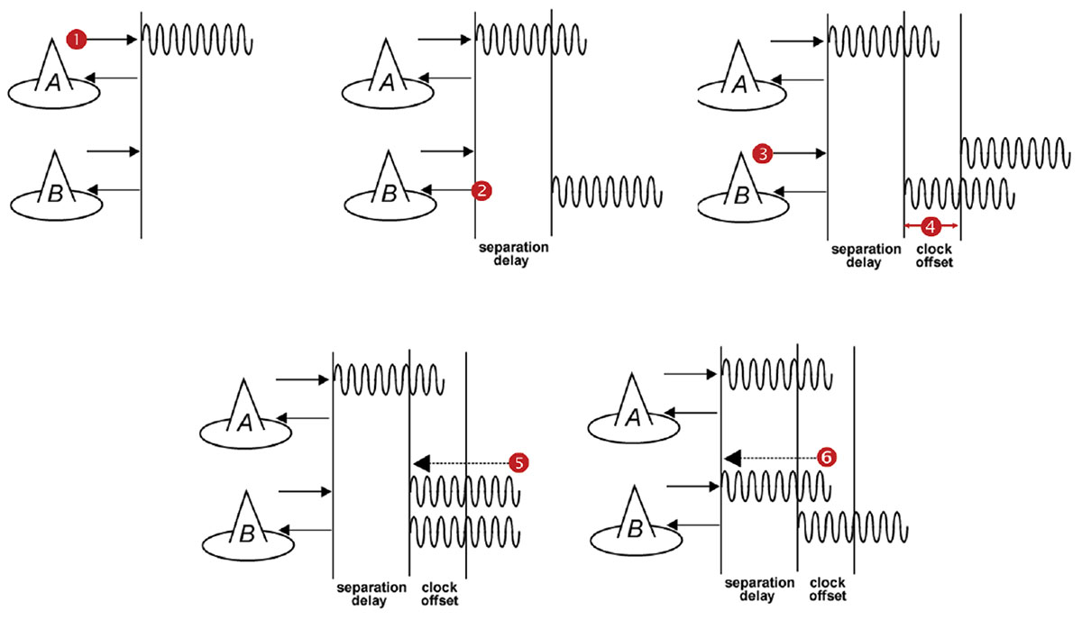
The TimeLoc Process

LocataNets function as local ground-based replicas of the satellite-based GPS position and timing networks. A LocataNet can be designed and configured by the user to deliver a powerful, local, controllable, tailored signal as required by different applications.

The easiest LocataNet layout to describe is a hub-and-spoke model consisting of a single master LocataLite transceiver and one or more slave LocataLites. More complex network configurations have been deployed in many commercial systems in use today. The patented process by which slaves are synchronized to the master (or other slaves) is known as TimeLoc.

In 2013, a University of New South Wales team demonstrated that Locata’s radio-based TimeLoc technology provided accurate time transfer (~5 ns) and frequency stability (~1 ppb) across a large distance of 73 kilometers (45.4 miles). This significantly outperforms GPS for wireless time transfer. Given this demonstrated radius of transmission in a rudimentary configuration, Locata was shown as being able to supply nanosecond-accurate time to a 146 km diameter circle, which would cover 16,750 km²— almost 200 times the size of Manhattan. Ranges greater than this can be deployed if required for safety-of-life, military or government-mandated systems.

As TimeLoc is accomplished without the use of atomic clocks, this represents a new level in precision network synchronization of this scale. It could conceivably serve as a GPS augmentation or back-up solution over wide areas for critical applications that depend on precise time.

Since Locata technology was originally developed as a high-accuracy non-GPS-based positioning and navigation solution, the time synchronization accuracy requirements for a LocataLite transceiver are very high. If sub-centimeter positioning precision is desired for a Locata receiver, every smallest fraction of a second is significant; for example, a 1-nanosecond error in time equates to an error of approximately 30 centimeters.

TimeLoc wireless synchronization enables LocataLites to achieve high levels of synchronization without atomic clocks, without external control cables, without differential corrections, and without a master reference receiver.

In theory, there is no limit to the number of LocataLites that can be synchronized together. TimeLoc allows a LocataNet to propagate into difficult environments or over wide areas. For example, if a third LocataLite C can only receive the signals from B (and not A) then it can use these signals from B for time synchronization instead. The only requirement for establishing a LocataNet using TimeLoc is that LocataLites must receive signals from one other LocataLite. This does not have to be the same central or master LocataLite, since this may not be possible in difficult environments with obstructions, or when propagating the LocataNet over wide areas.

This method of cascading TimeLoc through intermediate LocataLites has been proven in a growing number of real-world operational LocataNets, including a network in use today by the U.S. Air Force which is configured to cover up to 2,500 square miles (6,500 square kilometers) of the White Sands Missile Range in New Mexico.

In large networks where extremely high synchronization accuracies are required, it is useful to incorporate a meteorological sensor at each LocataLite to monitor the change in weather over considerable distances. This is certainly the case for long-range systems such as the USAF LocataNet installed at the huge White Sands Missile Range, where distances of over 50 km can be found between LocataLites. However, for the purposes of these USNO Washington experiments, where the longest point-to-point transmission distance was 2.9 km, it was assumed that weather parameters would be virtually identical at all LocataLite locations. Therefore only one MET station was employed within the entire network, which for these trials was collocated with the master LocataLite.

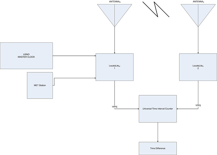
The very first experiment conducted by the USNO to gain some familiarization with TimeLoc was run entirely within the grounds of the USNO campus. It employed two LocataLites with their respective antennas on the roof of USNO Building 78. In this initial configuration the antennas were positioned 15.24 m apart. It was intended to use the measured result as a baseline against which TimeLoc synchronization over longer distance could be compared. This first arrangement is referred to as the two-node setup. A diagram of this configuration is shown in Figure 3.

Figure 3. Two-node setup (total range: 15.24 m/50 ft).

Second and third experiments demonstrated Locata’s ability to cascade the master 1PPS signal to an intermediary slave LocataLite, which in turn transmits a signal to which a third LocataLite can TimeLoc. This LocataNet configuration is referred to as the three-node setup (Figure 4).

Figure 4. Three-node setup (total range: 5.794 km/3.6 mi and 2.401 km/1.49 mi).

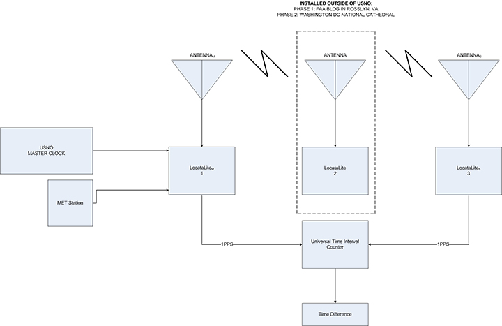
This experiment was conducted twice using two different intermediate LocataLite locations. The first intermediate location was indoors on the top floor of the FAA Building in Rosslyn, Va. (Figure 5). The distance between the master/slave antennas to the intermediate antenna in the FAA building was 2.897 km, but since the signal was propagated through a tinted window, the received signal strength inside the building was greatly attenuated, effectively simulating a much longer transmission distance. The second intermediate (LocataLite 2) location was from the balcony of the National Cathedral’s Ringing Chamber. In this case the distance between USNO LocataLite 1 master/slave to the intermediate antenna in the National Cathedral was approximately 1.183 km.

Figure 5. Intermediate LocataLite 2 antennas inside FAA building. In the distance, both the USNO and the National Cathedral are visible.

In both cases in Figure 4, the distance between master and terminal slave antennas was 3.048 m on the USNO building, but they were intentionally not TimeLoc’d to each other. The timing signal was therefore forced to route through the intermediate LocataLite 2 at either the FAA Building or the National Cathedral.

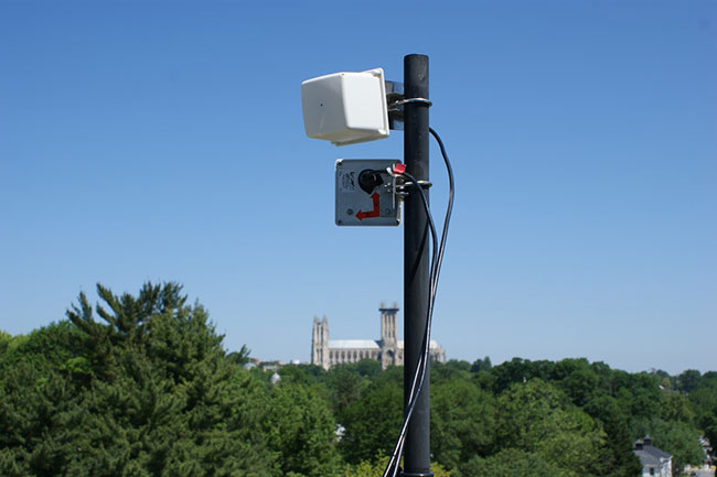
A fourth experiment included yet another intermediate cascade where the TimeLoc signal was transmitted from the second to a third LocataLite/antenna before arriving at the fourth LocataLite in the chain. This LocataNet configuration is referred to as the four-node setup. A diagram of the setup is shown in Figure 6, and it now added a LocataLite on USNO Building 1 to expand the set-up, along with the intermediate LocataLite installed at the National Cathedral (Figure 7).

Figure 6. Four-node setup (total range: 2.413 km/1.5 mi).

Figure 7. LocataLite antennas outside the Ringing Chamber of the National Cathedral Spire.

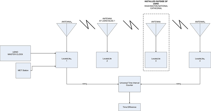
Referring to Figure 6, the distance between the master LocataLite (antenna 1) at USNO Building 78 and the LocataLite (antenna 2) at USNO Building 1 was approximately 42.672 m. The distance between the USNO Building 1 (antenna 2) to the Washington National Cathedral (antenna 3), was approximately 1.144 km. The distance between the Washington National Cathedral (antenna 3) back to antenna 4 on USNO Building 78 was approximately 1.183 km. The total range in this four-node chain was 2.413 km. In this configuration, LocataLites 1 and 4 are intentionally not TimeLoc’d to each other, forcing the 1PPS signal to be routed through LocataLites 2 and 3.

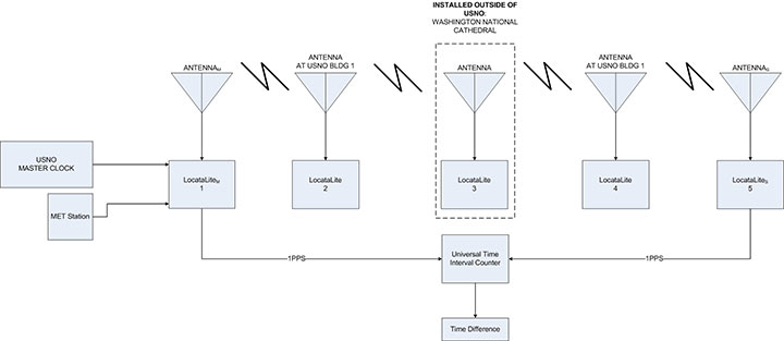
A fifth experiment included yet one more LocataLite and antenna at USNO Building 1 (Figure 9), totaling cascaded TimeLoc among five LocataLites and their respective antennas: the five-node setup, shown in Figure 8. In this configuration LocataLites 1 and 5 are intentionally not TimeLoc’d to each other, forcing the 1PPS signal to be routed through LocataLites 2, 3 and 4.

Figure 8. Five-node setup (total range: 2.427 km/1.51 mi).

Figure 9. LocataLite antennas on USNO Building 1. National Cathedral in background.

Measurement Methodology

A measurement of time difference between master and slave LocataLite 1PPS readings was done using a Stanford SR620 universal time interval counter. The rising edge of the 1PPS signals were inspected at 1-Volt trigger level. A 10 MHz reference was provided to the counter from the USNO’s Master Clock. Channels A and B on the counter were designated to the master and slave 1PPS signals respectively. Data were collected from the counter through serial connection to a PC. The length of each experiment was time-limited in some way because of limited access to facilities, such as the FAA building or National Cathedral. However, a minimum of at least 30,000 seconds (8.33 hours) of data were collected for each test to characterize the overall stability of the 1PPS signals between master and terminal slave LocataLites.

Collected Data

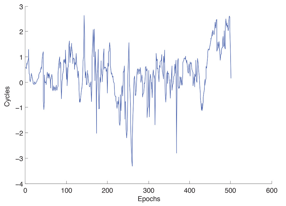
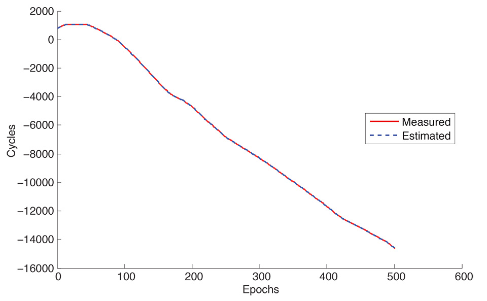
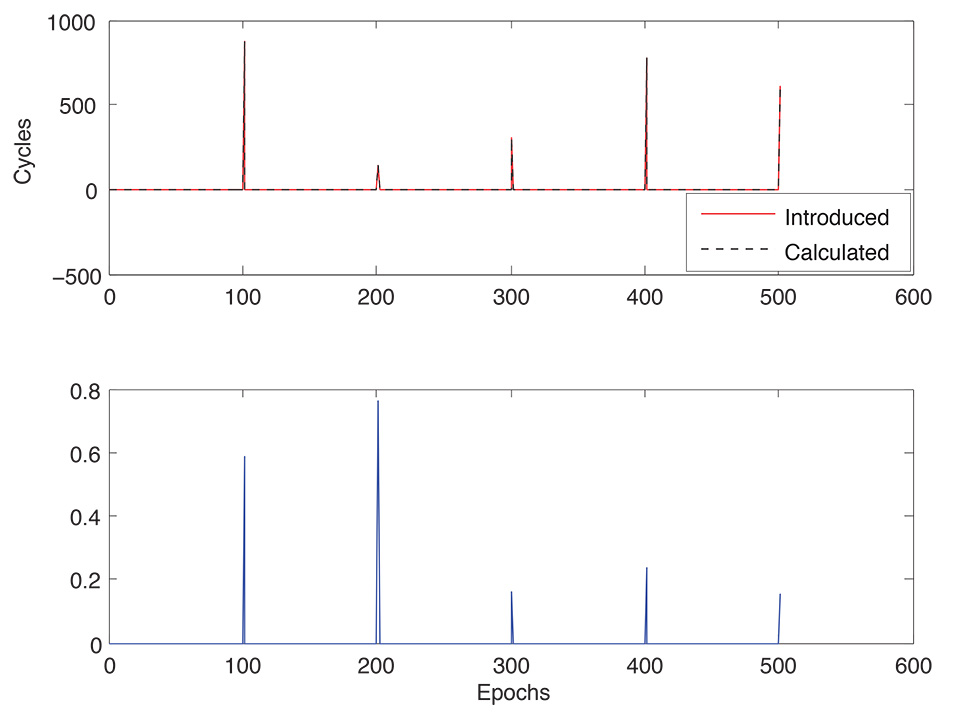
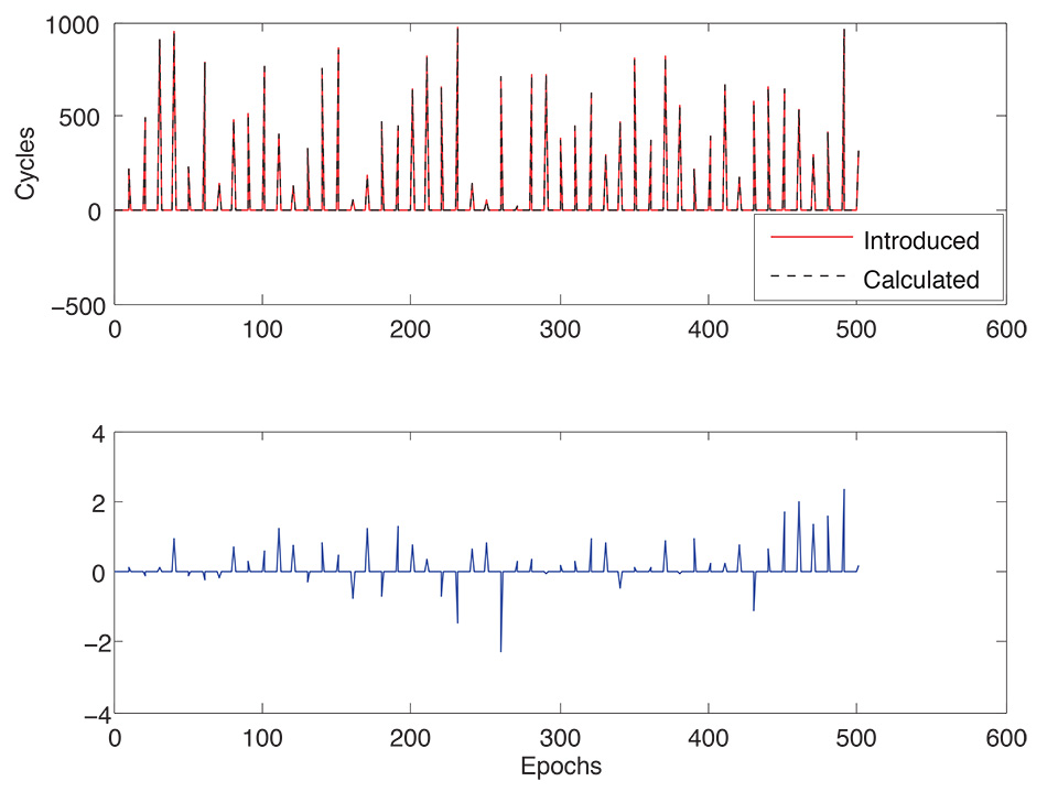
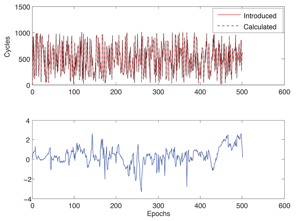
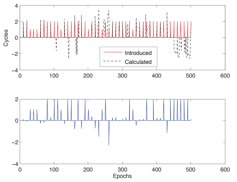
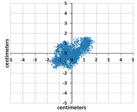
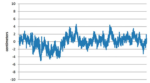
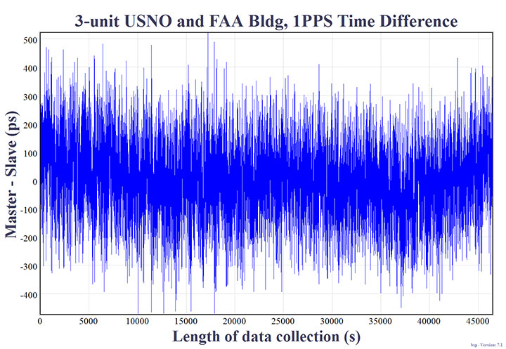
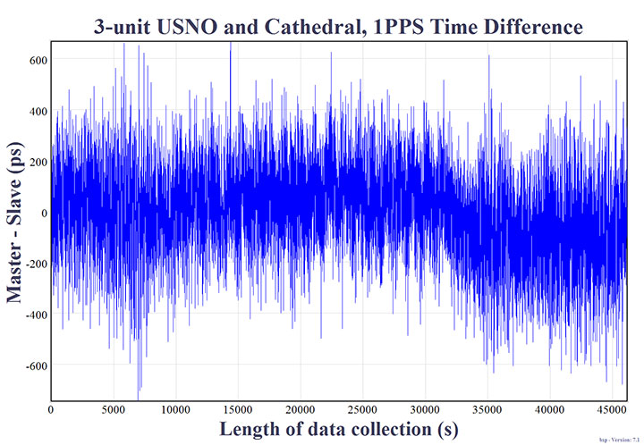
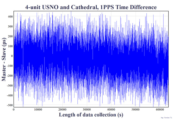
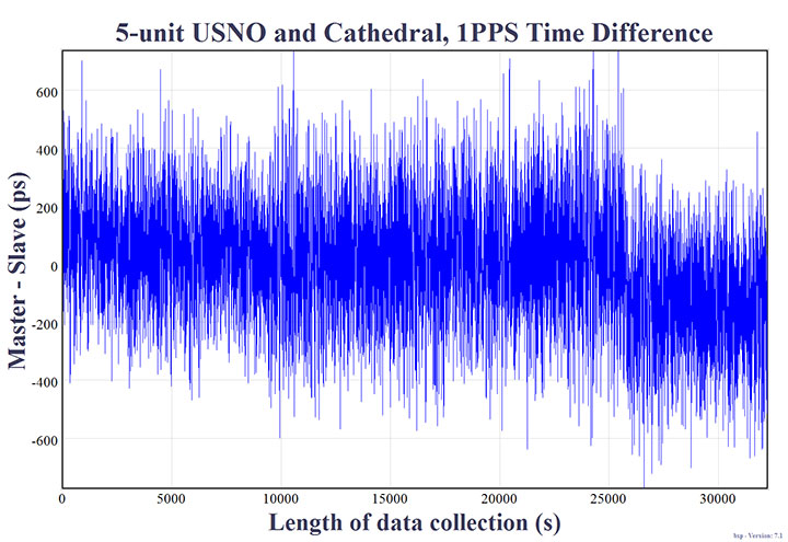
Figures 10 to 14 show the normalized 1PPS time difference between the master LocataLite and the terminal slave LocataLite. Normalization effectively removes errors due to unsurveyed antenna locations and uncorrected cable delays; hence it highlights the frequency coherence of the network.

Figure 10. Two-node setup on USNO rooftop, collected for slightly more than 1 day. Distance: 15.24 m/50 ft. Synchronization Standard Deviation (SSD) = 51.095 picoseconds.

Figure 11. Three-node setup at USNO and FAA Building, collected for over 12 hours: 5.794 km/3.6 mi. SSD = 127.333 picoseconds.

Figure 12. Three-node setup at USNO National Cathedral, collected for over 12-hours: 2.401 km/1.49 mi. SSD = 171.325 picoseconds.

Figure 13. Four-node setup at USNO with cascades at National Cathedral and USNO building 1, collected for over 17-hours: 2.413 km/1.5 mi. SSD = 145.247 picoseconds.

Figure 14. Five-node setup with cascades at National Cathedral and 2 hops at USNO building 1, collected for over 8-hours: 2.427 km/1.51 mi. SSD = 197.766 picoseconds.

Results

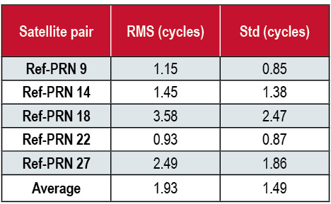
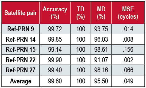
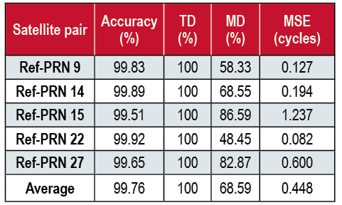
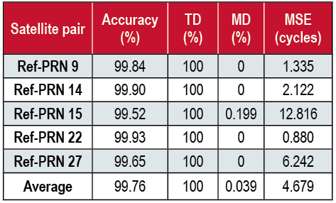
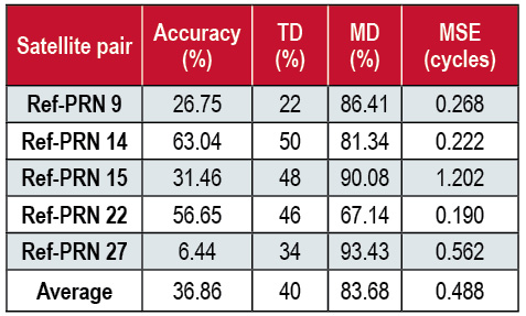
The results in Table 1 show the 1PPS signal variability for each LocataNet under evaluation. These values represent the frequency coherence between master and terminal slave LocataLite 1PPS signals for each experiment.

Table 1. LocataNet frequency stability.

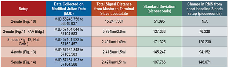
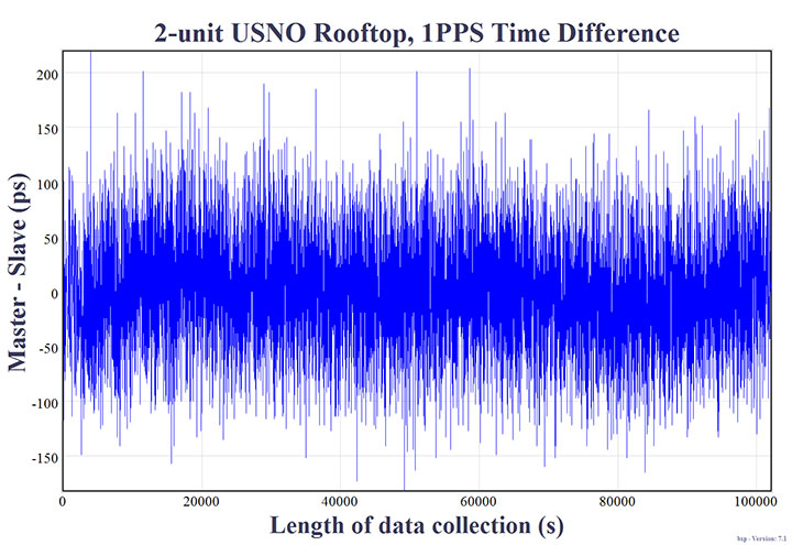
The two-node setup used two LocataLite antennas located within 15.24m of each other. The measured precision standard deviation was 51.095 picoseconds. This value is a culmination of the total Locata noise budget, which is expected to consist of TimeLoc noise, residual tropospheric error, multipath change (signal scattering/diffusion), PPS generation, and PPS measurement. This two-node result can be used as a baseline for Table 1 measurement results over longer distances. The differences are shown in the last column of Table 1. For example, cascading TimeLoc over the 5.794 km three-node setup introduced an additional deviation of 76.238 picoseconds, compared to the two-node set-up.

The three-node setup tested the effect of adding a TimeLoc cascade wherein the Locata signal from the master is routed to an intermediate LocataLite, and then to the terminal slave. When the master LocataLite signal was cascaded through the intermediate LocataLite at the FAA Building, the configuration showed a standard deviation of 127.333 ps across a total signal path length of 5.794 km. Alternatively, when the master LocataLite signal was cascaded through the intermediate LocataLite at the National Cathedral, that three-node configuration showed a standard deviation of 171.325 ps across a total signal path length of 2.401 km.

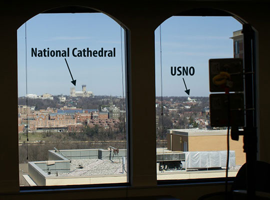
Interestingly, it appears that in the two different three-node setups, the intermediate cascade to the FAA building (2.9 km from the master and terminal slave LocataLites) delivered slightly better time transfer performance than the configuration which leveraged the closer (1.183 km) National Cathedral intermediate cascade. We believe this is attributable to the fact that the line-of-sight between USNO Building 78 (the site of the master and terminal slave) and the National Cathedral (the intermediate cascade) was completely obscured by heavy foliage seen in Figure 9, and that this particular configuration required the signal to pass through the foliage twice when being transmitted back and forth. Not only does foliage introduce multipath, but the properties of this foliage also changed regularly according to wind and moisture — two weather attributes that varied significantly over the course of the week in which those particular experiments were set up and run. This theory seems reasonable, since the four-node setup only required the signal to pass through this foliage once, and the recorded performance was better than the three-node setup — despite the fact that an additional TimeLoc cascade point was introduced.

The four-node setup included TimeLoc cascades at USNO Building 1 and the Washington National Cathedral. In this configuration, the data from Table 1 shows a standard deviation of 145.247ps across a total signal path length of 2.413 km.

The five-node setup included yet another TimeLoc cascade between the National Cathedral and Building 1 at USNO before reaching the terminal LocataLite slave. In this configuration, the data from Table 1 shows a standard deviation of 197.766ps across a total signal path length of 2.427 km.

Frequency Stability

Frequency stability is best measured over long periods. Because all of the equipment in the two-node setup was located on USNO premises, it could be run undisturbed for a longer period of time than configurations which required access to external facilities outside of the USNO’s control. Data obtained from the two-node setup were used to calculate the frequency stability between the two TimeLoc’d LocataLites. The length of this data set was 28 hours, 22 minutes, and 40 seconds. During this period, the approximate one-day frequency stability was measured as 1×10^-15(1 part per quadrillion).

To put this measurement into a more practical context: Stratum 1 is defined as a source of frequency with an accuracy of at least 1×10- 11, hence Stratum 1 performance generally originates from an atomic standard. For example, Cesium beam atomic clocks typically provide better performance than this, with one day Allen deviation stabilities in the mid- Ex10-14 (usually stable to between 3×10-14 to 6×10-14). Rubidium clocks are typically never more stable than 1×10-13 and Maser clocks are typically stable to mid-to-low Ex10-15 over one day.

Locata’s link stability — achieved without the use of atomic clocks — is clearly capable of distributing Stratum 1 frequency and precise time without substantially degrading the reference clock stability. This measured performance is significant, because a stable network is an essential prerequisite for precise time and frequency transfer. Moreover, for many traditional timing applications and developing digital and IoE applications, stability is more important than accuracy; just as for most advanced technology applications, frequency is more important than time of day.

Conclusions

The five USNO experiments suggest that the variations of the measured frequency synchronization between master and terminal slave LocataLites were not inevitably attributable to the distance between LocataLites, but rather governed by the number of nodes or cascade points in the LocataNet configuration, and LocataLite signal quality. Each signal cascade through an intermediate LocataLite introduced ~25ps of jitter into the solution.

Additionally, it was noted that transmitting TimeLoc signals across an urban environment did not always allow for unobstructed line-of-sight or completely open-sky environments. For instance, some of the LocataNet configurations required the signal to travel through dense, leafy trees which appeared to slightly affect overall frequency stability. Additionally, one FAA configuration required the signal to travel indoors through a tinted window which ultimately affected received signal strength.

These USNO tests highlighted the capability of the LocataLite as a viable option for a stable 1PPS distribution setup within an urban environment in support of applications like cell tower synchronization in “GPS-challenged” environments. All tested configurations demonstrated frequency synchronization of less than 200 picoseconds. This is significantly better than any other known wireless network synchronization methodology, including GPS. Furthermore, if clear line-of-sight is available between a master and slave LocataLite, the 2-node precision has been shown to be on the order of 50ps, and has one-day stabilities to 1×10-15.

These results, reinforced by those previously reported in University of New South Wales tests over a very large area, suggest that distance between nodes is not a significant factor, provided that sufficient signal quality is maintained. Thus, there are no theoretical or technical problems with scaling LocataNets to very large areas. In fact, this has already been demonstrated at the White Sands Missile Range where the USAF has now deployed a fully-operational Locata network that covers up to 2,500 square miles (6,500 square km), about 80 times the size of Manhattan.

The USNO trials reported here have clearly demonstrated TimeLoc’s relative picosecond-level synchronization of independent Locata networks. If this highly-stable network capability were not in place, precise time transfer would not be possible. The next step is to demonstrate how well a LocataNet can deliver absolute time transfer of the USNO’s Master Clock time to any other network node across similar areas of Washington, D.C.

Acknowledgments

The authors would like to thank James Shepherd of the National Cathedral and Paul Worcester of the FAA for use of their respective buildings. The authors would also like to thank Locata personnel for the use of their equipment and technical assistance in setting up the LocataNets under evaluation.

This article is based on a paper presented at ION GNSS+ 2015.

Disclaimer

Though particular vendor products are mentioned, neither official USNO endorsement nor recommendation of any product is herein implied.

Edward Powers is the GNSS and Network Time Transfer Operations Division Chief at USNO. He also serves as an advisor to the USAF GPS Directorate supporting space atomic clock development, modernized GPS III navigation message design, GPS accuracy improvement studies, and GPS UE development.

Arnold Colina is an electronics engineer in USNO’s GNSS and Network Time Transfer division, tasked with providing accurate UTC reference through GPS and performing calibration tests on GNSS receivers.

Timing Versus Synchronization

“They say “timing is everything” but nowadays it’s probably more correct to say “synchronization is everything”. There is a significant difference, yet many are surprised to learn they are not the same thing.

“Time dependent” applications rely on their clocks being close to the “real time”, as defined by a consensus of super-accurate atomic clocks managed by national bodies like the USNO. Once agreed upon by the labs, this “real time” can be distributed to various “time dependent” networks as a reference time to drive their operations.

“Time synchronized” applications, on the other hand, employ a methodology in which a common network time can be transferred to each network node. In other words, often the real technology enabler is that all the clocks in a defined network are synchronized to each other, even if they all run to what is any arbitrarily defined time-base. The “real time” doesn’t matter as much as how closely the node times agree with each other. As Einstein famously taught us: “Everything is relative.”

For example, accurate synchronization enables GPS positioning to work because a user’s GPS receiver relies on time-of-arrival comparisons from four or more satellites transmitting their signals at the same instant. But — even in this GPS paradigm where atomic clocks are always touted to be the most fundamental of requirements — it is important to appreciate this: A GPS user’s receiver does not care how, or to what “time,” the satellites are made synchronous. The only things the user receiver needs to know is where the satellites are, and that the satellites are synchronized when they transmit their signal.

Unfortunately sustaining high-precision, reliable time synchronization of multiple network nodes is a mammoth engineering task. Just ask the US Air Force! All clocks, no matter how accurate they are, eventually drift, so they cannot remain synchronized without comparison and adjustment.

Given the world’s exploding, insatiable demand for more data transmitted via ever-faster wireless systems, synchronization will become even more important than it is today. More wireless users and more bandwidth per user means that nanosecond — or even picosecond — network synchronization is one of the emerging engineering challenges of the 21st century. There are few resource on earth which are as scarce, or more precious today, than spectrum. So there is no question that better or cheaper ways to greatly improve network frequency and synchronization will translate directly into better use of the world’s exceptionally valuable, extremely limited spectrum resource.

October 5, 2015
Locata Positioning Will Underpin NASA’s Unmanned Aerial System Research 

NASA’s Ikhana is being used to test a system that will allow uncrewed aircraft to fly routine operations within the National Airspace System. (Credit: NASA)

NASA plans to install a Locata network (LocataNet) as the core positioning technology for safety-critical unmanned aerial systems (UAS) research at its Langley Research Center in Hampton, Va., according to an announcement by Locata.

NASA Langley is tasked with performing rigorous and repeatable scientific evaluation of new  UAS safety and technology concepts under development. The LocataNet will provide high-precision non-GPS-based positioning, navigation and timing (PNT) that is essential for this work. Known for its long history of aeronautics research, NASA Langley is a key center for UAS research and development. In June, one of Langley’s unmanned hexacopters (a drone with six rotors) delivered medical supplies to a clinic, the first such delivery by an unmanned drone.

Locata’s centimeter-accurate positioning will now assist NASA to develop and improve flight-critical technology systems that support air transportation safety, efficiency and performance. Langley’s extensive state-of-the-art facilities will be further enhanced with the installation of the LocataNet.

The NASA LocataNet is scheduled to be installed and commissioned before the end of 2015. Locata will supply the LocataLite Transmitters and Locata receivers required by NASA for the installation. Aviation-quality Locata antennas, developed by Cooper Antennas (UK) and previously used by the U.S. Air Force in its own military LocataNets, will also be installed. Locata engineers will support the physical installation, ongoing training and the future technical support required by NASA Langley for this world-first UAS deployment.

Locata Corporation has invented new terrestrial positioning networks which function as local, ground-based replicas of GPS. These networks can be thought of as “GPS hotspots,” according to the company. Locata has amassed 146 granted patents to date protecting these innovations, with many more patents in the works.

Locata is currently shipping commercial systems to demanding and professional end users such as the USAF, NASA, Leica Geosystems, and many others. Locata enables their integration partners to extend GPS-like positioning coverage to modern industrial, commercial, consumer and government applications in areas where GPS is erratic, jammed or unavailable.

“Locata is proud and delighted to have received an order for NASA’s first LocataNet. Globally significant installations like this prove Locata’s new technology is delivering unprecedented levels  of performance to many important new applications,” said Nunzio Gambale, Locata CEO. “As our technology roll-out begins to gain pace, the exceptional value Locata brings to next-gen mobile apps has attracted interest from players all over the world. In fact, our list of relationships is now looking like a roster of the world’s crème-de-la-crème. I honestly can’t think of a better or more prestigious name than NASA to add to our growing partner list.”

“Our team is savoring the opportunity to work alongside NASA engineers and we’re excited that Locata will help advance the safety-critical performance of Unmanned Aerial Systems,” he continued. “Almost all future mobile devices or machines, be they on the road, in the air, on a mine site, in a port, in a warehouse, in your mobile phone, or part of the inevitable Internet of Things — all of them are critically dependent on pervasive, reliable, high-accuracy positioning. Locata is being leveraged into these next-gen systems because it’s clear that satellite-based solutions alone can no longer deliver what’s required. Soon, as we bring miniaturized Locata transmitters and receivers to market, our innovations will enable even greater advances in cutting-edge consumer, commercial, and government applications.”

NASA Testing Program. As part of its UAS research, NASA is testing a system that would make it possible for unmanned aircraft to fly routine operations in United States airspace. Through the agency’s Unmanned Aircraft Systems Integration in the National Airspace System (UAS-NAS) project, NASA, General Atomics Aeronautical Systems, Inc. (GA-ASI) and Honeywell International, Inc., are flying a series of tests which began on June 17 and will run through July at NASA’s Armstrong Flight Research Center in California.

“We are excited to continue our partnership with GA-ASI and Honeywell to collect flight test data that will aid in the development of standards necessary to safely integrate these aircraft into the National Airspace System,” said Laurie Grindle, UAS-NAS project manager at Armstrong.

This is the third series of tests that builds upon the success of similar experiments conducted late last year that demonstrated a proof-of-concept sense-and-avoid system. The tests engage the core air traffic infrastructure and supporting software components through a live and virtual environment to demonstrate how a remotely piloted aircraft interacts with air traffic controllers and other air traffic.

“This is the first time that we are flight testing all of the technology developments from the project at the same time,” Grindle said.

This series of tests is made up of two phases. The first is focused on validation of sensor, trajectory and other simulation models using live data. Some of the tests will be flown with an Ikhana aircraft, based at Armstrong, that has been equipped with an updated sense-and-avoid system, as well as other advanced software from Honeywell.

Other tests will involve an S-3B plane from NASA’s Glenn Research Center in Cleveland, serving as a high-speed piloted surrogate aircraft. Both tests will use other aircraft following scripted flight paths to intrude on the flight path the remotely-piloted craft is flying, prompting it to either issue an alert or maneuver out of the other aircraft’s path. These flights will also conduct the first full test of the traffic alert and collision avoidance system (TCAS II) on a remotely piloted aircraft.

During the June 17 test, which lasted a little more than five hours, the team accomplished 14 encounters using the Ikhana aircraft and a Honeywell-owned Beech C90 King Air acting as the intruder. A second test was flown the following day, with a total of 23 encounters. The project team plans to fly more than 200 encounters throughout the first phase of the test series.

“Our researchers and project engineers will be gathering a substantial amount of data to validate their pilot maneuver guidance and alerting logic that has previously been evaluated in simulations,” said Heather Maliska, Armstrong’s UAS-NAS deputy project manager.

The second phase of the third test series will begin in August and will include a T-34 plane equipped with a proof-of-concept control and non-payload communications system. It will evaluate how well the systems work together so that the aircraft pilots itself, interacts with air traffic controllers and remains well clear of other aircraft while executing its operational mission. The aircraft, which will have an onboard safety pilot, will fly an operationally representative mission in a virtual airspace sector complete with air traffic control and live and virtual traffic.

August 6, 2015
eDLoran: The Next-Gen Loran
Potential GNSS Back-up Improves to GPS-Level Accuracy

A new enhanced differential Loran system demonstrates 5-meter accuracy not achievable by the current DLoran system, and requires less expensive reference stations. A prototype tested in Rotterdam’s Europort area uses standard mobile telecom networks and the Internet to reduce correction data latency — a key source of error — by one to two orders of magnitude.

By Durk van Willigen, René Kellenbach, Cees Dekker, and Wim van Buuren

For maritime applications, Loran is considered as the most promising backup for GNSS for situations where the use of navigation satellite signals is denied. For this reason, the Dutch Pilots’ Corporation askedReelektronika to investigate whether differential Loran could meet the Dutch Pilots’ 5-meter accuracy requirement for a harbor navigation system. This proved to be an enormous challenge, as preliminary tests showed that even 10 meters was difficult to achieve with differential Loran (DLoran) as promoted by Trinity House, the UK lighthouse authority. This led to a thorough renewed investigation of all possible error sources of a complete differential Loran system. The outcome of this research is very promising, as a couple of major error sources could be isolated. This made the complete system better understandable, so adequate countermeasures could be taken.

Loran History

The development of Loran-C started in the United States about fifty years ago. It is a terrestrial low-frequency (100 kHz) system organized as chains, each consisting of a master station with two or more secondary stations. Each station broadcasts in a strict time format series of 8 or 9 pulses of approximately 250 µs. The effective radiated power is in the range of 100 to 1,000 kW, depending on the required working range. These high powers are required by the high levels of atmospheric noise in the 100 kHz frequency band.

Figure 1 shows the test area of enhanced Differential Loran (eDLoran), using the Loran stations of Lessay (France), Sylt (Germany), and Anthorn (UK).

Figure 1. The Loran configuration in the test area of Europort.

Radiating such high-power pulses requires large vertical transmitting antennae of about 200 meters height (Figure 2). These high power levels have long been seen as a drawback of Loran-C. However, the upcoming GNSS interference risks changed this apparent drawback into an advantage, as jamming such high field strengths is hardly achievable unnoticed. Loran-C is, unfortunately, less accurate than GNSS but it is nearly impossible to jam over large areas. This is one of the major reasons that Loran gets so much renewed interest by all who face risks in life-critical and environment-critical applications of radio navigation.

Figure 2. Left, the antenna park of 13 masts of ≈200 meters at Anthorn, UK. Right, the 200-meter mast at Sylt, Germany.

Differential Loran

Standard Loran does not meet accuracy requirements for harbor entrance and approaches. The International Maritime Organization requires 10 meters (95 percent), which is at least 5 times more demanding than standard Loran can provide. So, differential techniques have been developed and implemented, which are comparable with differential GPS. Although the error sources of GPS and Loran are quite different, the major common error source in both systems is the lack of accurate propagation models.

Several years ago, the General Lighthouse Authorities (GLAs) of the UK and Ireland implemented Differential Loran (DLoran) in the test area around Harwich. DLoran is based on a Loran reference station in the area of interest which measures temporal deviations of the measured pseudoranges. These “errors” are then sent to the user receiver through the Eurofix Loran Data Channel. This technique strongly resembles that of differential GPS. Unfortunately, for a number of reasons it proved to be impossible to achieve absolute accuracies of better than 10 meters with DLoran.

This has led to a new research project to find a more accurate differential Loran technique. All possible error sources have been investigated again where possible, producing unexpected solutions regarding accuracy and cost.

Error Sources

The total position error of Loran depends on the accuracy in time of the high-power generated Loran pulses feeding the antenna, the stability of the physical phase center of the Loran transmitter antenna, stability of the tuning of the antenna circuit, the accuracy of the measured additional secondary phase factor stored in the Additional Secondary Factor (ASF)database, and the quality of the Loran receiver. ASF is the additional delay when Loran signals propagate over land with a varying conductivity. As the ASF data are not fixed but vary slightly over time, temporal de-correlation, differential techniques have been developed to counteract that effect. In standard DLoran systems, the differential corrections are sent to the user through the Eurofix data link. Particular error sources include:

Transmitter Timing Accuracy. A Loran transmitter sends about 100 pulses per second. Each station has three cesium clocks time-synchronized to Coordinated Universal Time (UTC) via a time-transfer network. A two-way satellite time-transfer system will make it simpler and more accurate.

Antenna Phase-Center Stability. Loran transmitter antennas are vertical towers approximately 200 meters high to provide vertical polarization. Its phase center, at the published position, does not move more than about 1 meter according to the station crew at Sylt.

This situation is very different for a wire antenna as installed at the station at Anthorn in Northern England. The top-loaded wire antenna is installed between two towers 200 meters tall and separated by 675 meters (Figure 3). In stormy weather, the antenna position is not stable and does not continuously coincide within 1 meter of the published position of the antenna.

Figure 3. The enormous top-loaded Loran wire antenna at Anthorn. This type of antenna is not rigidly stable during storm. By courtesy of Babcock International Group.

ASF Data. The net travel time of the Loran signal from the transmitter to the receiver antenna is the sum of the propagation through the atmosphere (primary factor or PF), some extra delay due to traveling over seawater (secondary factor or SF), and finally ASF. The PF and SF are calculated from models, while the ASF must be measured. These calculations can only be accurate if the net travel time can be accurately determined and the distance between transmitter and receiver can be calculated with the help of GPS-RTK. The time stamps of the signal when leaving the antenna are not sufficiently accurate. The time stamps on the received signals are established by using a GPS-disciplined rubidium (Rb) clock. In conclusion, we cannot accurately measure and compute the absolute ASF values. All mentioned possible errors led to the use of differential techniques.

Differential Loran

As it is not possible to measure ASF data to sufficient accuracy, time-stamp errors at the transmitter can be circumvented by applying differential techniques over a limited area of interest. The receiver at the reference site and the rover receiver experience the same transmitter timing error, which makes it a common error and harmless in differential Loran. It is more difficult to cope with the offset of the Rb clocks at the reference and the rover sites, which is, unfortunately, not common-mode. Differential clock errors of a moving rover receiver may easily rise to 20 ns, equivalent to 6 meters. This type of error limits the achievable accuracy of an ASF data base.

The measured/calculated ASF data are due to weather effects on propagation slightly moving with time. That is the reason to use a reference receiver to measure these temporal variations and send these as AFS corrections to the rover receiver via the 30 bps Eurofix data link. Unfortunately, this rather slow data link introduces significant data latency, which turned out to be the source of significant differential Loran errors.

In the UK, many tests have been conducted to measure these ASF shifts and use the Eurofix data link for sending correction data to the user receiver. DLoran data are sent as pseudorange corrections per station. A complete set of DLoran correction data takes about 90 seconds. The UK plans to send correction data from multiple reference stations via a single Eurofix channel. The resulting very large data latency will preclude accuracies any better than 10 meters. The main reason of this conclusion was found by further analysis of measurements of the position of the rover receiver. These positions are shown as a scatter plot in Figure 4.

Figure 4. On the left the position deviation scatter plot at the rover receiver. The middle plot is the result after applying DLoran corrections from a reference station. The right plot of the same DLoran plot after being low-pass filtered indicating the slow moving of the phase center of the Anthorn transmitter. The axes are in meters.

The left-hand plot gives the position deviation of 2,500 independent measurements, where the scattering was thought to be caused by noise on the measurements. The middle plot is the result after being corrected by DLoran data with a 90-second data latency, which shows a somewhat modified form but still quite noisy plot. However, when the DLoran data were low-pass filtered, it appeared that often all separate measurements more or less formed lines, which would not happen with just atmospheric noise. Further, the scattering after filtering did not decrease much, which would happen if the disturbances were due to noise. See the right-hand plot in Figure 4.

This demonstrates that the source of the problem is the slow data rate through the Eurofix channel, in combination with the movements of the phase center of the transmitter antenna at Anthorn. Apparently, the solution had to be found in a much faster data link which could neither be offered by Eurofix (30 bps) nor by the U.S.-proposed OFDM technique with a data rate of approximately 1 kb/s. This unexpected result forced us to drastically change the concept of differential Loran to get much better accuracy results, as requested by the Rotterdam pilots.

Enhanced Differential Loran

The above mentioned difficulties with DLoran have led to a new concept of differential Loran which had to fulfil three important primary improvements. The first is a significant reduction in the latency of the data in the data channel; the second is that a large number of reference stations should be allowed to send correction data to the user without saturating the data channel. Finally, it is necessary to measure ASF data more accurately without being dependent on atomic clocks.

The simple conclusion was that Eurofix could not meet the first two improvements. As Eurofix is an invention of Delft University in the Netherlands, it was somewhat painful for the Dutch to admit that a much faster data link is absolutely needed to achieve a two-fold better differential Loran position accuracy. However, Eurofix is still the prime GNSS backup candidate for distributing accurate UTC over very large parts of Europe. Further, Eurofix has the capability to send short messages, which might be encrypted for secure communication purposes that might then form a terrestrial backup for Galileo PRS.

Finally, the third improvement to generate more accurate ASF data cannot be found on a pseudorange method but has to be established on position bases.

Instead of using the Eurofix channel, eDLoran uses the public Global System for Mobile (GSM) network to send the differential corrections to users. eDLoran receivers therefore contain a simple modem for connection to the GSM network. The eDLoran reference stations are also connected to the Internet, which may be implemented via a cabled access or also via a GSM modem.

Fortunately, today many GSM networks are robust in respect of GPS outages. The eDLoran concept is quite simple and is shown in Figure 5.

Figure 5. Concept of eDLoran. By courtesy of Babcock International Group.

The eDLoran infrastructure is not connected with any Loran transmitter station and operates completely autonomously. An eDLoran reference station is connected to a central eDLoran server by its connection to the Internet.

The measured positions of these reference receivers are processed in the eDLoran server, which returns the resulting correction data to the user, also via the Internet. Data latency will be not more than 2 seconds. The rover receiver starts the entire process by sending the raw position to the server, which will then return the optimal ASF database for that particular area. Corrections can be calculated by using data from multiple reference stations. Reference stations for eDLoran are small and consume not more than 10 Watts. Two types of reference stations are under development. A portable simple battery-powered version, not larger than 2 meters, can operate for 8 hours. This version is meant to do interference analysis on selected candidate locations. For a permanent installation, a continuously operating solar-powered unit is also under development. See Figure 6.

Figure 6. Concepts of a mini reference station (left) and a permanent eDLoran reference station.

It has been mentioned that measuring accurately the departure and arrival times of Loran pulses is difficult. It is however needed in order to work out the ASF data on the pseudorange measurement for each Loran station in view. Therefore, a DLoran ASF measurement receiver concept uses Rb clocks and is relatively large and power-hungry. With eDLoran, position offsets due to ASF effects are measured and an eDLoran reference server outputs position- instead of pseudorange-corrections. Measuring positions is much simpler and more accurate and can be done with standard miniature low-power eLoran receivers. No GPS-disciplined Rb clock is needed, and total costs are significantly lower. The gain in accuracy of this simpler ASF measurement receiver together with the very low data latency is one of the reasons that the resulting eDLoran position accuracy is now approximately 5 meters instead of 10 meters with DLoran.

eDLoran Results

We conducted real-life static and dynamic tests to demonstrate the capabilities of this new concept. The static tests were done in post-processing with logged data from Hook of Holland and at Reelektronika, about 40 kilometers to the east. Only standard eLoran receivers, mostly equipped with E-field antennae, were used, and no atomic clocks were applied. At Reelektronika ,we used two 2-meter mini-reference stations, while in Hook of Holland the Loran antenna was mounted on top of the 30-meter lighthouse. Dynamic tests were done on board of the MS Polaris, the new pilot-station vessel of the Dutch Pilots’ Corporation.

Static Tests. To give a realistic image of the resulting errors of eDLoran, the scatter plots in Figures 7 and 8 are depicted in the position domain. The radial errors are shown in the time domain where the horizontal axis gives the 5-second epochs. The left and the middle plot show the results of the rover and the reference receiver, respectively. The eDLoran plots on the right depict interesting results, as those variations in ASF are largely cancelled while the scattering is smaller than that of the measurements at the rover and the reference receiver, individually. The scattering at the two locations was apparently partly due to low-frequency disturbances, for example because of the moving phase center of the antenna at Anthorn, or instabilities in the time-control loops in the transmitters.

Figure 7. Position scatter plots in the upper row and radial error plots in the lower row of the user receiver on the Maasvlakte and the reference receiver at Hook of Holland. The right-hand column depicts the results for eDLoran. The two sites are separated by about 11 km. The horizontal axis shows the 5-second epochs.

Figure 8. Position scatter plots in the upper row and radial error plots in the lower row of the receivers at Reelektronika and Hook of Holland. The right-hand column depicts the results for eDLoran. The two sites are separated by about 40 km. Some eDLoran accuracy degradation around events 250 and 500 may be due to local interference at Reelektronika.

Figure 7 shows the situation where the rover and the reference receiver were separated by 11 kilometers, while Figure 8 depicts the results when the rover receiver was at Reelektronika, more than 40 kilometers from the reference site at Hook of Holland.

This effect of movement of the phase center of the transmitter antenna is further made visible by applying an alpha-tracker (α = 0.9) on the position data of both receivers, which have an update rate of 5 seconds. The lining-up of dots on some parts of the scatter plots in Figure 9 are believed to be due to swaying of the transmitter antenna. Due to the low-pass filtering, the disturbances now contain fewer high-frequency terms.

Investigating the radial error plots of Figure 9, it is remarkable that the large excursions at event 1880 largely cancelled. The disturbance at event 1880 might be caused by antenna movement at Anthorn, which is nearly perfectly cancelled by eDLoran.

Figure 9. Above plots are based on the same data as in Figure 8 but now after passing through an alpha tracker with α = 0.9. Note the correlation of the radial deviations around events 1800 in both 40 km separated receivers and the strong reduction in scattering.

Investigating the radial error plots of Figure 8 and 9, it is remarkable that the large excursions around epoch 1900 largely cancel, while this is not happening at epoch 250. There, some local interference might have been the cause. The disturbance at event 1900 might be caused by swaying of the Anthorn antenna which is then a common-mode error at both receivers and is therefore strongly reduced in the eDLoran plots.

Dynamic Tests. Dynamic testing on board the Polaris at sea (Figure 10) is somewhat more complex to do correctly. The eDLoran receiver was installed about 1 meter above the GPS-RTK reference receiver. In this way, the lever-arm problem of not installing the antennae of the two receivers at the same location was avoided. The next issue was measuring ASF position data, which should happen synchronously with the GPS measurements. Time synchronization can be achieved by using simple GPS receivers at both Loran receivers. Some months later, the eDLoran concept was tested by using the stored AFS data and using a Reelektronika eDLoran receiver as a portable pilot unit (PPU) which looks identical to the GPS-based units the Rotterdam pilots use, manufactured by AD Navigation in Norway.

Figure 10. Top right, the Pilot Station Vessel MS Polaris (80 meters) used to test eDLoran (photo copyright Loodswezen). Below is a complete eDLoran receiver with a ‘life-line’ connected to avoid losing the receiver by accident and to allow charging the internal batteries.

Figure 11. Five test antennae on the MS Polaris. From left to right the ADNav Master Processing Unit, the ADNav Heading Unit, the ADNav Position Unit with the Reelektronika eDLoran receiver 1 meter above it and, finally, a second Reelektronika eDLoran receiver.

The results have been demonstrated to the harbor authorities in real-time on the laptop of the pilots on which the GPS-RTK and the eDLoran position were simultaneously shown. See Figure 12, where the large gray ship model represents the position and heading derived from GPS-RTK. The width of the ship model is 10 meters. The red triangle gives the eDLoran position; it remains within the borders of the ship symbol. For further demonstration purposes, the logged GPS-RTK data could also be plotted on a Google Earth map (Figure 13). The track was widened to 10 meters, as the accuracy requirements are 5 meters on either side of the track. The raw eLoran track is also shown, as well as the final white eDLoran track of unfiltered raw eDLoran data, which stays well within the 5-meter boundaries.

Figure 12. The large ship symbol (grey) is derived from the GPS-RTK receiver of the Rotterdam pilots. The width of the ship symbol is 10 meters and the speed-over-ground was 11 kts. The red triangle is generated by the eDLoran receiver and remains between the required ± 5 meter limits for eDLoran.

Figure 13. The red track is based on raw eLoran data without any corrections. The transparent blue line is made by GPS-RTK and is widened to 10 meters giving the required ± 5 meter limits of eDLoran. The white line is output from the eDLoran receiver which stays within the borders of the 10 meter wide transparent blue line.

During the sea trials, the eDLoran receiver was connected to the eDLoran server on land via a miniature GSM modem to the Internet. All differential data were read via this mobile link. The required data bandwidth is very low, approximately 150 bps per ship (client).

Conclusions

The outcome of this research opens some new and quite surprising possibilities for multiple applications:
- eDLoran offers the best possible eLoran accuracy, as it does not suffer from unstable transmitter antennas, sub-optimal timing control of the transmitter station, and differential data latency.
- There is no need to replace older Loran-C stations with eLoran transmitters; this potentially would save large amounts of money. Further savings may be obtained by containerizing the transmitter and operating the stations unmanned.
- Installing eDLoran reference stations is fast, simple, and very cost-effective.
- The Eurofix Loran Data Channel can be freed from a relatively large stream of DLoran data, which leaves the full data bandwidth available for UTC and short-message services over very large areas.
- As there is no data channel bandwidth limitation, multiple reference stations can be installed, offering increased reliability and making the system more robust to terrorism and lightning damage.
- Single or multiple eDLoran servers can be installed in a protected area. There is hardly a practical limit to the number of differential reference stations to serve.
- The server selects the most optimal differential data based on the raw position of the user (client) and the available reference stations.
- As there is no need for any Loran data channel, eDLoran can be installed in all locations where Loran or Chayka coverage and access to the Internet are available. Required data bandwidth is approximately 150 bps per user.
- Standard eLoran receivers used on controlled trajectories (for example, pilots and ferries) collect position data when accurate DGNSS is available. The collected GNSS and eLoran data can be uploaded to the server to further refine the ASF data base. It is basically a self-learning system.
- All eDLoran reference stations monitor the eLoran and GNSS positions to offer alarm services in case of GNSS jamming or spoofing.
Acknowledgments We are very grateful for the near-endless hospitality of the Rotterdam Pilots and especially the crew of the MS Polaris and the MS Markab. Without their help, we would not have obtained the eDLoran results presented here. During the days at sea, we learned how much experience and professionalism is needed to bring those extremely large vessels safely in the harbor of Rotterdam.

We thank Martin Rumens and Dave Kelleher of Babcock International Group for their valued comments and diagrams.

DURK VAN WILLIGEN is a retired professor of electronic systems for navigation at the Delft University of Technology. He is founder and president of Reelektronika B.V., and started the development of Eurofix in 1985. He received the Thurlow Navigation Award of the Institute of Navigation (U.S.) and the Gold Medal of the Royal Institute of Navigation (UK).

RENÉ KELLENBACH graduated from Delft University of Technology in electrical engineering. After joining Reelektronika as a systems engineer, he has been involved in designing hardware and software for radionavigation and radar systems.

CEES DEKKER graduated from the Delft University of Technology in electrical engineering. He worked previously at Philips Research Labs and now assists Reelektronika B.V. with the development of Loran systems and GPS-related projects, and information systems.

WIM VAN BUUREN is a licensed maritime pilot in Rotterdam who took the initiative to develop a backup positioning system for the approaches to Rotterdam. He has been involved in the design and development of the hardware and software of Portable Pilot Units on a national and European level since 2000.
June 28, 2014
Out in Front: How Much Farther?
For some years now, we have been talking about GNSS interoperability. The concept has received so much careful attention at conferences, in R&D laboratories, in international working group forums, and behind closed high-level government and military doors, that one might understandably conclude that we have talked interoperability into existence.

Not quite. Not nearly. Not by the farthest, if measuring into the next decade constitutes far, reach of our actual, real-world grasp.

“If you can imagine it, you can achieve it.” William Arthur Ward, a professional inspirer of the 20th century, said that.

For nearly as many years now, we have been talking about GPS and GNSS backup. Similarly, the concept has undergone careful examination and much repeated (’til blue in the face) urging and warning and alarum-
sounding and planning and conjecturing and running through the halls of Congress. One might understandably conclude that we have conjured backup for critical infrastructure into actual, tangible, effective existence.

Again, not quite.

“Everybody talks about GPS backup, but nobody does anything about it.” Mark Twain said that.

April’s GLONASS downfall prompted distinguished industry leaders to again take up cudgels for multi-GNSS and for redundant PNT. They deserve and require our support, on all fronts, whether in the public arena, the lab, or the marketplace. But neither concept yet exists, truly and pervasively, that is to say effectively for all users.

When will reliable, robust, consistent and continuous positioning, navigation, and timing become a reality? Should we rely on whatever technology we currently possess until the perfect system comes available, or should we continuously upgrade at each iterative step along the way?

We take up this topic in our June 5 webinar, “How Much Farther to the Promised Land? Purchase Decisions in the Evolving Landscape of GPS, Multi-GNSS, and Alternative PNT.”

Four speakers will present:
- a high-precision GNSS manufacturer,
- a mass-market GNSS manufacturer,
- an alternative PNT provider,
- a design and manufacturing firm,
followed by questions from you, our audience. Come for a glimpse into the future, and estimations of its distance and time of travel from current location.

Among the key insights: technology changes too fast to wait until the next generation of a product to add new capabilities, when doing so risks loss of competitive edge or, worse, risks introducing a new product already obsolete. A mid-lifecycle component change can deliver both greater performance and cost savings. For details on this prior to June 5, visit the White Paper section of our website.
May 1, 2014
Innovation: Cycle Slips

Detection and Correction Using Inertial Aiding

By Malek O. Karaim, Tashfeen B. Karamat, Aboelmagd Noureldin, Mohamed Tamazin, and Mohamed M. Atia

A team of university researchers has developed a technique combining GPS receivers with an inexpensive inertial measuring unit to detect and repair cycle slips with the potential to operate in real time.

INNOVATION INSIGHTS by Richard Langley

DRUM ROLL, PLEASE. The “Innovation” column and GPS World are celebrating a birthday. With this issue, we have started the 25th year of publication of the magazine and the column, which appeared in the very first issue and has been a regular feature ever since. Over the years, we have seen many developments in GPS positioning, navigation, and timing with a fair number documented in the pages of this column.

In January 1990, GPS and GLONASS receivers were still in their infancy. Or perhaps their toddler years. But significant advances in receiver design had already been made since the introduction around 1980 of the first commercially available GPS receiver, the STI-5010, built by Stanford Telecommunications, Inc. It was a dual-frequency, C/A- and P-code, slow-sequencing receiver. Cycling through four satellites took about five minutes, and the receiver unit alone required about 30 centimeters of rack space. By 1990, a number of manufacturers were offering single or dual frequency receivers for positioning, navigation, and timing applications. Already, the first handheld receiver was on the market, the Magellan NAV 1000. Its single sequencing channel could track four satellites. Receiver development has advanced significantly over the intervening 25 years with high-grade multiple frequency, multiple signal, multiple constellation GNSS receivers available from a number of manufacturers, which can record or stream measurements at data rates up to 100 Hz. Consumer-grade receivers have proliferated thanks, in part, to miniaturization of receiver chips and modules. With virtually every cell phone now equipped with GPS, there are over a billion GPS users worldwide. And the chips keep getting smaller. Complete receivers on a chip with an area of less than one centimeter squared are common place. Will the “GPS dot” be in our near future?

The algorithms and methods used to obtain GPS-based positions have evolved over the years, too. By 1990, we already had double-difference carrier-phase processing for precise positioning. But the technique was typically applied in post-processing of collected data. It is still often done that way today. But now, we also have the real-time kinematic (or RTK) technique to achieve similar positioning accuracies in real time and the non-differenced precise point positioning technique, which does not need base stations and which is also being developed for real-time operation. But in all this time, we have always had a “fly in the ointment” when using carrier-phase observations: cycle slips. These are discontinuities in the time series of carrier-phase measurements due to the receiver temporarily losing lock on the carrier of a GPS signal caused by signal blockage, for example. Unless cycle slips are repaired or otherwise dealt with, reduction in positioning accuracy ensues. Scientists and engineers have developed several ways of handling cycle slips not all of which are capable of working in real time. But now, a team of university researchers has developed a technique combining GPS receivers with an inexpensive inertial measuring unit to detect and repair cycle slips with the potential to operate in real time. They describe their system in this month’s column.

“Innovation” is a regular feature that discusses advances in GPS technology and its applications as well as the fundamentals of GPS positioning. The column is coordinated by Richard Langley of the Department of Geodesy and Geomatics Engineering, University of New Brunswick. He welcomes comments and topic ideas.

GPS carrier-phase measurements can be used to achieve very precise positioning solutions. Carrier-phase measurements are much more precise than pseudorange measurements, but they are ambiguous by an integer number of cycles. When these ambiguities are resolved, sub-centimeter levels of positioning can be achieved.

However, in real-time kinematic applications, GPS signals could be lost temporarily because of various disturbing factors such as blockage by trees, buildings, and bridges and by vehicle dynamics. Such signal loss causes a discontinuity of the integer number of cycles in the measured carrier phase, known as a cycle slip. Consequently, the integer counter is reinitialized, meaning that the integer ambiguities become unknown again. In this event, ambiguities need to be resolved once more to resume the precise positioning and navigation process. This is a computation-intensive and time-consuming task. Typically, it takes at least a few minutes to resolve the ambiguities.

The ambiguity resolution is even more challenging in real-time navigation due to receiver dynamics and the time-sensitive nature of the required kinematic solution. Therefore, it would save effort and time if we could detect and estimate the size of these cycle slips and correct the measurements accordingly instead of resorting to a new ambiguity resolution. In this article, we will briefly review the cause of cycle slips and present a procedure for detecting and correcting cycle slips using a tightly coupled GPS/inertial system, which could be used in real time. We will also discuss practical tests of the procedure.

Cycle Slips and Their Management

A cycle slip causes a jump in carrier-phase measurements when the receiver phase tracking loops experience a temporary loss of lock due to signal blockage or some other disturbing factor. On the other hand, pseudoranges remain unaffected. This is graphically depicted in FIGURE 1. When a cycle slip happens, the Doppler (cycle) counter in the receiver restarts, causing a jump in the instantaneous accumulated phase by an integer number of cycles. Thus, the integer counter is reinitialized, meaning that ambiguities are unknown again, producing a sudden change in the carrier-phase observations.

FIGURE 1. A cycle slip affecting phase measurements but not the pseudoranges.

Once a cycle slip is detected, it can be handled in two ways. One way is to repair the slip. The other way is to reinitialize the unknown ambiguity parameter in the phase measurements. The former technique requires an exact estimation of the size of the slip but could be done instantaneously. The latter solution is more secure, but it is time-consuming and computationally intensive. In our work, we follow the first approach, providing a real-time cycle-slip detection and correction algorithm based on a GPS/inertial integration scheme.

GPS/INS Integration

An inertial navigation system (INS) can provide a smoother and more continuous navigation solution at higher data rates than a GPS-only system, since it is autonomous and immune to the kinds of interference that can deteriorate GPS positioning quality. However, INS errors grow with time due to the inherent mathematical double integration in the mechanization process. Thus, both GPS and INS systems exhibit mutually complementary characteristics, and their integration provides a more accurate and robust navigation solution than either stand-alone system. GPS/INS integration is often implemented using a filtering technique. A Kalman filter is typically selected for its estimation optimality and time-recursion properties.

The two major approaches of GPS/INS integration are loosely coupled and tightly coupled. The former strategy is simpler and easier to implement because the inertial and GPS navigation solutions are generated independently before being weighted together by the Kalman filter. There are two main drawbacks with this approach: 1) signals from at least four satellites are needed for a navigation solution, which cannot always be guaranteed; and 2) the outputs of the GPS Kalman filter are time correlated, which has a negative impact upon the system performance. The latter strategy performs the INS/GPS integration in a single centralized Kalman filter. This architecture eliminates the problem of correlated measurements, which arises due to the cascaded Kalman filtering in the loosely coupled approach. Moreover, the restriction of visibility of at least four satellites is removed. We specifically use a tightly coupled GPS/reduced inertial sensor system approach.

Reduced Inertial Sensor System. Recently, microelectromechanical system or MEMS-grade inertial sensors have been introduced for low-cost navigation applications. However, these inexpensive sensors have complex error characteristics.

Therefore, current research is directed towards the utilization of fewer numbers of inertial sensors inside the inertial measurement unit (IMU) to obtain the navigation solution.

The advantage of this trend is twofold. The first is avoidance of the effect of inertial sensor errors. The second is reduction of the cost of the IMU in general. One such minimization approach, and the one used in our work, is known as the reduced inertial sensor system (RISS). The RISS configuration uses one gyroscope, two accelerometers, and a vehicle wheel-rotation sensor. The gyroscope is used to observe the changes in the vehicle’s orientation in the horizontal plane. The two accelerometers are used to obtain the pitch and roll angles. The wheel-rotation sensor readings provide the vehicle’s speed in the forward direction. FIGURE 2 shows a general view of the RISS configuration.

FIGURE 2. A general view of the RISS configuration.

A block diagram of the tightly coupled GPS/RISS used in our work is shown in FIGURE 3. At this stage, the system uses GPS pseudoranges together with the RISS observables to compute an integrated navigation solution. In this three-dimensional (3D) version of RISS, the system has a total of nine states. These states are the latitude, longitude, and altitude errors ( ; the east, north, and up velocity errors ; the azimuth error ; the error associated with odometer-driven acceleration ; and the gyroscope error .

The nine-state error vector x_k at time t_k is expressed as:
    (1)

FIGURE 3. Tightly coupled integration of GPS/RISS using differential pseudorange measurements.

Cycle Slip Detection and Correction

Cycle slip handling usually happens in two discrete steps: detection and fixing or correction. In the first step, using some testing quantity, the location (or time) of the slip is found. During the second step, the size of the slip is determined, which is needed along with its location to fix the cycle slip. Various techniques have been introduced by researchers to address the problem of cycle-slip detection and correction. Different measurements and their combinations are used including carrier phase minus code (using L1 or L2 measurements), carrier phase on L1 minus carrier phase on L2, Doppler (on L1 or L2), and time-differenced phases (using L1 or L2). In GPS/INS integration systems, the INS is used to predict the required variable to test for a cycle slip, which is usually the true receiver-to-satellite range in double-difference (DD) mode, differencing measurements between a reference receiver and the roving receiver and between satellites. In this article, we introduce a tightly coupled GPS/RISS approach for cycle-slip detection and correction, principally for land vehicle navigation using a relative-positioning technique.

Principle of the Algorithm. The proposed algorithm compares DD L1 carrier-phase measurements with estimated values derived from the output of the GPS/RISS system. In the case of a cycle slip, the measurements are corrected with the calculated difference. A general overview of the system is given in FIGURE 4.

FIGURE 4. The general flow diagram of the proposed algorithm.

The number of slipped cycles is given by
   (2)
where
is the DD carrier-phase measurement (in cycles)
is DD estimated carrier phase value (in cycles).
is compared to a pre-defined threshold μ . If the threshold is exceeded, it indicates that there is a cycle slip in the DD carrier-phase measurements.

Theoretically, would be an integer but because of the errors in the measured carrier phase as well as errors in the estimations coming from the INS system, will be a real or floating-point number.

The estimated carrier-phase term in Equation (2) is obtained as follows:
    (3)
where
λ is the wavelength of the signal carrier (in meters)
are the estimated ranges from the rover to satellites i and j respectively (in meters)
are known ranges from the base to satellites i and j respectively (in meters).
What we need to get from the integrated GPS/RISS system is the estimated range vector from the receiver to each available satellite ( ). Knowing our best position estimate, we can calculate ranges from the receiver to all available satellites through:
(4)
where
is the calculated range from the receiver to the mth satellite
x^KF is the receiver position obtained from GPS/RISS Kalman filter solution
x^m is the position of the mth satellite
M is the number of available satellites.
Then, the estimated DD carrier-phase term in Equation (3) can be calculated and the following test quantity in Equation (2) can be applied:
   (5)
If a cycle slip occurred in the ith DD carrier-phase set, the corresponding set is instantly corrected for that slip by:
   (6)
where s is the DD carrier-phase-set number in which the cycle slip has occurred.

Experimental Work

The performance of the proposed algorithm was examined on the data collected from several real land-vehicle trajectories. A high-end tactical grade IMU was integrated with a survey-grade GPS receiver to provide the reference solution. This IMU uses three ring-laser gyroscopes and three accelerometers mounted orthogonally to measure angular rate and linear acceleration. The GPS receiver and the IMU were integrated in a commercial package. For the GPS/RISS solution, the same GPS receiver and a MEMS-grade IMU were used. This IMU is a six-degree of freedom inertial system, but data from only the vertical gyroscope, the forward accelerometer, and the transversal accelerometer was used. TABLE 1 gives the main characteristics of both IMUs. The odometer data was collected using a commercial data logger through an On-Board Diagnostics version II (OBD-II) interface. Another GPS receiver of the same type was used for the base station measurements. The GPS data was logged at 1 Hz.

Table 1. Characteristics of the MEMS and tactical grade IMUs.

Several road trajectories were driven using the above-described configuration. We have selected one of the trajectories, which covers several real-life scenarios encountered in a typical road journey, to show the performance of the proposed algorithm. The test was carried out in the city of Kingston, Ontario, Canada. The starting and end point of the trajectory was near a well-surveyed point at Fort Henry National Historic Site where the base station receiver was located. The length of the trajectory was about 30 minutes, and the total distance traveled was about 33 kilometers with a maximum baseline length of about 15 kilometers. The trajectory incorporated a portion of Highway 401 with a maximum speed limit of 100 kilometers per hour and suburban areas with a maximum speed limit of 80 kilometers per hour. It also included different scenarios including sharp turns, high speeds, and slopes.

FIGURE 5 shows measured carrier phases at the rover for the different satellites. Some satellites show very poor presence whereas some others are consistently available. Satellites elevation angles can be seen in FIGURE 6.

FIGURE 5. Measured carrier phase at the rover.

FIGURE 6. Satellite elevation angles.

Results

We start by showing some results of carrier-phase estimation errors. Processing is done on what is considered to be a cycle-slip-free portion of the data set for some persistent satellites (usually with moderate to high elevation angles). Then we show results for the cycle-slip-detection process by artificially introducing cycle slips in different scenarios. In the ensuing discussion (including tables and figures), we show results indicating satellite numbers without any mention of reference satellites, which should be implicit as we are dealing with DD data.

FIGURE 7 shows DD carrier-phase estimation errors whereas FIGURE 8 shows DD measured carrier phases versus DD estimated carrier phases for sample satellite PRN 22.

FIGURE 7. DD-carrier-phase estimation error, reference satellite with PRN 22.

FIGURE 8. Measured versus estimated DD carrier phase, reference satellite with PRN 22.

As can be seen in TABLE 2, the root-mean-square (RMS) error varies from 0.93 to 3.58 cycles with standard deviations from 0.85 to 2.47 cycles. Estimated phases are approximately identical to the measured ones. Nevertheless, most of the DD carrier-phase estimates have bias and general drift trends, which need some elaboration. In fact, the bias error can be the result of more than one cause. The low-cost inertial sensors always have bias in their characteristics, which plays a major role in this. The drift is further affecting relatively lower elevation angle satellites which can also be attributed to more than one reason. Indeed, one reason for choosing this specific trajectory, which was conducted in 2011, was to test the algorithm with severe ionospheric conditions as the year 2011 was close to a solar maximum: a period of peak solar activity in the approximately 11-year sunspot cycle.

Table 2. Estimation error for DD carrier phases (in cycles).

Moreover, the time of the test was in the afternoon, which has the maximum ionospheric effects during the day. Thus, most part of the drift trend must be coming from ionospheric effects as the rover is moving away from the base receiver during this portion of the trajectory. Furthermore, satellite geometry could contribute to this error component. Most of the sudden jumps coincide with, or follow, sharp vehicle turns and rapid tilts. Table 2 shows the averaged RMS and standard deviation (std) DD carrier-phase estimation error for the sample satellite-pairs. We introduced cycle slips at different rates or intensities and different sizes to simulate real-life scenarios. Fortunately, cycle slips are usually big as mentioned earlier and this was corroborated by our observations from real trajectory data. Therefore, it is more important to detect and correct for bigger slips in general.

Introducing and Detecting Cycle Slips. To test the robustness of the algorithm, we started with an adequate cycle slip size. Cycle slips of size 10–1000 cycles were introduced with different intensities. These intensities are categorized as few (1 slip per 100 epochs), moderate (10 slips per 100 epochs), and severe (100 slips per 100 epochs). This was applied for all DD carrier-phase measurement sets simultaneously. The threshold was set to 1.9267 (average of RMS error for all satellite-pairs) cycles. Four metrics were used to describe the results. Mean square error (MSE); accuracy, the detected cycle slip size with respect to the introduced size; True detection (TD) ratio; and Mis-detection (MD) ratio. Due to space constraints and the similarity between results for different satellites, we only show results for the reference satellite with PRN 22. FIGURES 9–12 show introduced versus calculated cycle slips along with the corresponding detection error for sample satellites in the different scenarios. TABLES 3–5 summarize these results.

FIGURE 9. Introduced and calculated cycle slips (upper plot) and detection error (lower plot). Few cycle slips case, reference satellite with PRN 22.

FIGURE 10. Introduced and calculated cycle slips (upper plot) and detection error (lower plot). Moderate cycle slips case, reference satellite with PRN 22.

FIGURE 11. Introduced and calculated cycle slips (upper plot) and detection error (lower plot). Intensive cycle slips case, reference satellite with PRN 22.

FIGURE 12. Introduced and calculated cycle slips (upper plot) and detection error (lower plot). Small cycle slips case, reference satellite with PRN 22.

Table 3. Few slips (1 slip per 100 epochs).

Table 4. Moderate slips (10 slips per 100 epochs).

Table 5. Intensive slips (100 slips per 100 epochs).

All introduced cycle slips were successfully detected in all of the few, moderate, and severe cases with very high accuracy. A slight change in the accuracy (increasing with higher intensity) among the different scenarios shows that detection accuracy is not affected by cycle-slip intensity. Higher mis-detection ratios for smaller cycle-slip intensity comes from bigger error margins than the threshold for several satellite pairs. However, this is not affecting the overall accuracy strongly as all mis-detected slips are of comparably very small sizes. MD ratio is zero in the intensive cycle-slip case as all epochs contain slips is an indicator of performance compromise with slip intensity.

It is less likely to have very small cycle slips (such as 1 to 2 cycles) in the data and usually it will be hidden with the higher noise levels in kinematic navigation with low-cost equipment. However, we wanted to show the accuracy of detection in this case. We chose the moderate cycle slip intensity for this test. TABLE 6 summarizes results for all satellites.

Table 6. Small slips (1–2 cycles) at moderate intensity (10 slips per 100 epochs).

We get a moderate detection ratio and modest accuracy as the slips are of sizes close to the threshold. The MSE values are not far away from the case of big cycle slips but with higher mis-detection ratio.

Conclusions

The performance of the proposed algorithm was examined on several real-life land vehicle trajectories, which included various driving scenarios including high and slow speeds, sudden accelerations, sharp turns and steep slopes. The road testing was designed to demonstrate the effectiveness of the proposed algorithm in different scenarios such as intensive and variable-sized cycle slips.

Results of testing the proposed method showed competitive detection rates and accuracies comparable to existing algorithms that use full MEMS IMUs. Thus with a lower cost GPS/RISS integrated system, we were able to obtain a reliable phase-measurement-based navigation solution. Although the testing discussed in this article involved post-processing of the actual collected data at the reference station and the rover, the procedure has been designed to work in real time where the measurements made at the reference station are transmitted to the rover via a radio link. This research has a direct influence on navigation in real-time applications where frequent cycle slips occur and resolving integer ambiguities is not affordable because of time and computational reasons and where system cost is an important factor.

Acknowledgments

This article is based on the paper “Real-time Cycle-slip Detection and Correction for Land Vehicle Navigation using Inertial Aiding” presented at ION GNSS+ 2013, the 26th International Technical Meeting of the Satellite Division of The Institute of Navigation held in Nashville, Tennessee, September 16–20, 2013.

Manufacturers

The research reported in this article used a Honeywell Aerospace HG1700 AG11 tactical-grade IMU and a NovAtel OEM4 GPS receiver integrated in a NovAtel G2 Pro-Pack SPAN unit, a Crossbow Technology (now Moog Crossbow) IMU300CC MEMS-grade IMU, an additional NovAtel OEM4 receiver at the base station, a pair of NovAtel GPS-702L antennas, and a Davis Instruments CarChip E/X 8225 OBD-II data logger.

Malek Karaim is a Ph.D. student in the Department of Electrical and Computer Engineering of Queen’s University, Kingston, Ontario, Canada.

Tashfeen Karamat is a doctoral candidate in the Department of Electrical and Computer Engineering at Queen’s University.

Aboelmagd Noureldin is a cross-appointment professor in the Departments of Electrical and Computer Engineering at both Queen’s University and the Royal Military College (RMC) of Canada, also in Kingston.

Mohamed Tamazin is a Ph.D. student in the Department of Electrical and Computer Engineering at Queen’s University and a member of the Queen’s/RMC NavINST Laboratory.

Mohamed M. Atia is a research associate and deputy director of the Queen’s/RMC NavINST Laboratory.

FURTHER READING

• Cycle Slips

“Instantaneous Cycle-Slip Correction for Real-Time PPP Applications” by S. Banville and R.B. Langley in Navigation, Vol. 57, No. 4, Winter 2010–2011, pp. 325–334.

“GPS Cycle Slip Detection and Correction Based on High Order Difference and Lagrange Interpolation” by H. Hu and L. Fang in Proceedings of PEITS 2009, the 2nd International Conference on Power Electronics and Intelligent Transportation System, Shenzhen, China, December 19–20, 2009, Vol. 1, pp. 384–387, doi: 10.1109/PEITS.2009.5406991.

“Cycle Slip Detection and Fixing by MEMS-IMU/GPS Integration for Mobile Environment RTK-GPS” by T. Takasu and A. Yasuda in Proceedings of ION GNSS 2008, the 21st International Technical Meeting of the Satellite Division of The Institute of Navigation, Savannah, Georgia, September 16–19, 2008, pp. 64–71.

“Instantaneous Real-time Cycle-slip Correction of Dual-frequency GPS Data” by D. Kim and R. Langley in Proceedings of KIS 2001, the International Symposium on Kinematic Systems in Geodesy, Geomatics and Navigation, Banff, Alberta, June 5–8, 2001, pp. 255–264.

“Carrier-Phase Cycle Slips: A New Approach to an Old Problem” by S.B. Bisnath, D. Kim, and R.B. Langley in GPS World, Vol. 12, No. 5, May 2001, pp. 46-51.

“Cycle-Slip Detection and Repair in Integrated Navigation Systems” by A. Lipp and X. Gu in Proceedings of PLANS 1994, the IEEE Position Location and Navigation Symposium, Las Vegas, Nevada, April 11–15, 1994, pp. 681–688, doi: 10.1109/PLANS.1994.303377.

Short-Arc Orbit Improvement for GPS Satellites by D. Parrot, M.Sc.E. thesis, Department of Geodesy and Geomatics Engineering Technical Report No. 143, University of New Brunswick, Fredericton, New Brunswick, Canada, June 1989.

• Reduced Inertial Sensor Systems

“A Tightly-Coupled Reduced Multi-Sensor System for Urban Navigation” by T. Karamat, J. Georgy, U. Iqbal, and N. Aboelmagd in Proceedings of ION GNSS 2009, the 22nd International Technical Meeting of the Satellite Division of The Institute of Navigation, Savannah, Georgia, September 22–25, 2009, pp. 582–592.

“An Integrated Reduced Inertial Sensor System – RISS / GPS for Land Vehicle” by U. Iqbal, A. Okou, and N. Aboelmagd in Proceedings of PLANS 2008, the IEEE/ION Position Location and Navigation Symposium, Monterey, California, May 5–8, 2008, pp. 1014–1021, doi: 10.1109/PLANS.2008.4570075.

• Integrating GPS and Inertial Systems

Fundamentals of Inertial Navigation, Satellite-based Positioning and their Integration by N. Aboelmagd, T. B. Karmat, and J. Georgy. Published by Springer-Verlag, New York, New York, 2013.

Aided Navigation: GPS with High Rate Sensors by J. A. Farrell. Published by McGraw-Hill, New York, New York, 2008.

Global Positioning Systems, Inertial Navigation, and Integration, 2nd edition, by M.S. Grewal, L.R. Weill, and A.P. Andrews. Published by John Wiley & Sons, Inc., Hoboken, New Jersey, 2007.

January 1, 2014
UrsaNav Accepts Delivery of First Production Nautel NL40 eLoran Transmitter

UrsaNav’s President, Charles Schue, shown accepting the transmitter from Nautel’s President, Peter Conlon.

After extensive Final Acceptance Testing at Nautel’s Hackett’s Cove, NS facility, UrsaNav has accepted delivery of the first production NL40 Loran-C and Enhanced Loran (eLoran) transmitter. This seventh-generation Loran transmitter technology is the culmination of more than six years of collaborative development between the two companies.

The transmitter successfully met or exceeded all of the requirements of the U.S. Coast Guard “Specification of the Transmitted Loran-C Signal.” Testing was conducted into a simulated antenna matching the characteristics of a U.S. Coast Guard “standard” 625-foot top-loaded monopole. The NL-Series transmitters are capable of transmitting Loran-C, eLoran, Chayka, and eChayka in any combination at power levels exceeding one megawatt. They are qualified for today, and prepared for tomorrow, UrsaNav said.

“Resilient PNT begins with complementary technologies, layered one upon the other in such a way that the user is ensured improved continuity of operations over a sole-source solution,” said UrsaNav President Charles Schue. “eLoran is the terrestrial co-primary complement to GNSS, and our technology makes eLoran the most economical, efficient, and wide-area alternative when GNSS is not available.”

November 19, 2013
Moving the Game Forward: Transceivers Aboard Light Vehicles

By John Carr and James Earl

Perspectives from a senior technical specialist and a production engineer at Newmont Boddington Gold Mine.

Newmont Fleet Management Services now continually monitors and plots the performance of JPS Locata alongside traditional GNSS in an effort to fine-tune the installed infrastructure. Learning to sculpt the perfect network continues as we move our JPS LocataLite transmitters to accommodate an ever-changing and expanding pit design.

Large twelve-meter benches and an aggressive mining plan have seen both North Pit and South Pit at NBG rapidly increase in depth, bringing the problems associated with GPS coverage in a deep-pit environment.

As mine sites develop and evolve, for the first time ever, we have the ability to dictate and control which areas we direct our own positioning coverage, and guarantee we can sustain accurate high-precision navigation wherever we need it. This level of control has just never been available before, and is literally impossible with satellite-based positioning signals. With GPS you just get what you get.

We are rapidly re-evaluating what may now be possible. We believe we are only at the very beginnings of where we can go with the LocataNet in the mining environment.

See also:
Synchronized Ground Networks Usher in Next-Gen GNSS

Staying One Step Ahead. Shape changes from week to week keep operations continuously relocating around the mine benches; this can, in some instances, make optimal positioning of the Jps LocataNet challenging. In the early stages of the project, we relied on producing computer-generated radio-coverage heat-map models of the pit to determine optimum positions for the individual LocataLite transmitters on the pit rim, and this is still a valid path if given the time.

However, with more Jps rovers becoming available, we now tend to make highly accurate predictions about network configuration on the fly. We can now install spare rovers as portable units in light vehicles (LVs) used by technicians onsite. This roaming functionality allows use of the Jps web browser in the rover to instantly validate, in the pit, any changes that may be required for the network before drilling and digging equipment is moved into place. Thus we can monitor real-world signal conditions in specific areas and adjust LocataLite positions to optimize positioning availability for machines that will soon arrive.

The typical network monitoring scenario nowadays is to quickly move a JPS-enabled LV onto a bench or area yet to be drilled or excavated, and review the signals from the individual LocataLite transmitters in real time. Technicians then make any necessary placement changes to the network in advance of any mining equipment arriving. Our ability to now ensure maximum possible positioning and navigation coverage at all times was undreamt of even 12 months ago.

Dual Rover. A modified HP Leica Drill JS System utilizing a Dual Jps Locata Rover has been installed into the drilling supervisors’ LV wagon. The drilling superintendent and supervisors had been exploring ways of moving towards a paperless system that could not only check the drill pattern itself, but also the areas being mined around the pattern. They identified a use-case example where having accurate positional information available in a vehicle enables supervisors to quickly review the construction and positioning of the protective windrows around the drill patterns. Access tracks and bench heights could also be checked without needing to call surveyors in to help. This degree of instantaneous clarity removes the guesswork associated with windrow construction, designed to provide a safety barrier between trucking and drilling operations. Incorrectly placed windrows can lead to potential flow restrictions in either operation, so getting it right the first time in active areas is important.

Mark-up by Night. Drilling supervisors can now accurately measure and monitor progress across the drill patterns using Locata technology to display virtual maps of all active drilling areas. Another spin-off benefit has been the introduction of a fixed point mounted to the front vehicle bullbar, to provide emergency mark-up of patterns during the nightshift when surveyors are not available on site. This helps particularly when a localized Wi-Fi outage prevents drills from downloading the blast pattern to commence drilling operations in an area of the mine. Before Jps, use of this high-precision GPS technology in vehicle had been considered ineffective and impractical because of the unreliable GPS coverage in the bottom of both pits. Plans are now under way to install a similar system into the shovel and auxiliary supervisors’ vehicles.

Forward! Recent group discussions found consensus that the best way to move forward with this technology now is continued integration into GPS, rather than stand-alone systems. Miners are generally a cautious lot: we could hedge our bets through a combined GPS+Locata solution package. Full-scale integration of Locata technology into future standard GPS products is perceived as a way companies such as NovAtel can provide the total package. We envisage a unified system available from all positioning receiver manufacturers that combines the benefits of GPS technology with the evident improvements and back-up that Locata has provided for environments where GPS is unable to function.

We have been in the enviable position of gaining a glimpse into the future, when the power of GPS-style positioning is improved to fill the GPS holes. The results we have obtained are, frankly, addictive. Having experienced this revolution first-hand, it would now be extremely painful to even contemplate going back to our previous GPS-only world.

October 1, 2013
Synchronized Ground Networks Usher in Next-Gen GNSS
LocataLite installation showing Jps transceiver tower.

Locata Fills Satellite Availability Holes in Obstructed Environments

By Chris Rizos, Nunzio Gambale, and Brendon Lilly

An integrated GNSS+Locata system installed on drills, shovels, and bulldozers — the full complement of high-precision machines on site — at Australia’s Newmont Boddington Gold Mine has increased positioning accuracy and availability, as well as mine operational efficiencies, demonstrating an improvement in availability over GNSS-only of 75.3 to 98.7 percent.

Many of the new paradigms in mining have at their core the requirement for reliable, continuous centimeter-level positioning accuracy to enable increased automation of mining operations. The deployment of precision systems for navigating, controlling, and monitoring machinery such as drills, bulldozers, draglines, and shovels with real-time position information increases operational efficiency, and the automation reduces the need for workers to be exposed to hazardous conditions.

GPS singly, and GNSS collectively, despite their accuracy and versatility, cannot satisfy the stringent requirements for many applications in mine surveying, and mine machine guidance and control. Increasingly, open-cut mines are getting deeper, reducing the sky-view angle necessary for GNSS to operate satisfactorily.

A new terrestrial high-accuracy positioning system can augment GNSS with additional terrestrial signals to enable centimeter-level accuracy, even when there are insufficient GNSS (GPS+GLONASS) satellite signals in view for reliable positioning and navigation. Locata relies on a network of synchronized ground-based transceivers that transmit positioning signals that can be tracked by suitably equipped user receivers.

In September 2012, Leica Geosystems launched the first commercial product integrating GNSS and Locata capabilities into a single high-accuracy and high-availability positioning device for open-cut mine machine automation applications: Leica Jigsaw Positioning System (Jps) – Powered by Locata. This article describes technical aspects of this technology and presents positioning results of actual mine operations.

In the near future — perhaps by 2020 — the number of GNSS and augmentation system satellites useful for high-accuracy positioning will increase to almost 150, with perhaps six times the number of broadcast signals on which carrier phase and pseudorange measurements can be made. However, the most severe limitation of GNSS performance will still remain: the accuracy of positioning deteriorates very rapidly when the user receiver loses direct view of the satellites. This typically occurs in deep open-cut mines as well as in skyscraper-dominated urban canyons.

Locata’s positioning technology solution provides an option either to augment GNSS with extra terrestrial signals, or to replace GNSS entirely. Locata relies on a network of synchronized ground-based transceivers (LocataLites) that transmit positioning signals that can be tracked by suitably equipped user receivers. These transceivers form a network (LocataNet) that can operate in combination with GNSS, or entirely independent of GNSS.

See also:
Moving the Game Forward: Transceivers Aboard Light Vehicles

Next-Generation Positioning

Pseudolites are ground-based transmitters of GPS-like signals. Most pseudolites developed to date transmit signals at the GPS frequency bands. Both pseudorange and carrier-phase measurements can be made on the pseudolite signals. The use of pseudolites can be traced back to the early stages of GPS development in the late 1970s, when they were used to validate the GPS concept before launch of the first GPS satellites.

In 1997, Locata Corporation began developing a technology to provide an alternate local GPS signal capability that would overcome many of the limitations of pseudolite-based positioning systems by using a time-synchronized transceiver. The LocataLite transmits GPS-like positioning signals but also can receive, track, and process signals from other LocataLites. A network of LocataLites forms a LocataNet, and the first-generation system transmitted signals using the same L1 frequency as GPS. Time-synchronized signals allow carrier-phase single-point positioning with centimeter-level accuracy for a mobile unit. In effect, the LocataNet is a new constellation of signals, with some unique features such as having no base station data requirement, requiring no wireless data link from reference station to mobile receiver, and no requirement for measurement double-differencing.

Improvements dating from 2005 use a proprietary signal transmission structure that operates in the license-free Industry Scientific and Medical (ISM) band (2.4–2.4835GHz), known globally as the Wi-Fi band. Within this ISM band, the LocataLite design allows for the transmission of two frequencies, each modulated with two spatially-diverse PRN codes. From the beginning the driver for the Locata technology was to develop a centimeter-level accuracy positioning system that could complement, or replace, conventional RTK-GNSS in environments such as open-cut mines, deep valleys, heavily forested areas, urban and even indoor locations, where obstruction of satellite-based signals occurs.

Leica Geosystems has been testing Locata in the Newmont Boddington Gold Mine (NBG) in Western Australia for several years. In 2006, NBG started installing Leica Geosystems high-precision GPS-based guidance systems for fleet management. The mine operators determined early on that as the pit grew deeper, they would need an alternative positioning system for these guidance systems to continue working for the life of the mine. In March 2012, Leica Geosystems deployed a world-first production version of its Jigsaw Positioning system, integrating GNSS+Locata, at the NBG mine.

Expected to become Australia’s largest gold producer, the mine consists of two pits (Figure 1). The North Pit at NBG is currently about 1 kilometer long, 600 meters wide, and now approaching 275 meters deep.

Figure 1. Location of 12 LocataLites at NBG Mine.

Figure 2. The Newmont Boddington pit, 900 feet deep and going deeper all the time, creates difficulties for GNSS equipment positioning the mine’s heavy machinery.

A single LocataNet consisting of 12 LocataLites was deployed during April and May 2012 in an initial installation designed to cover both pits in the mine. The results presented here are taken from tests in the North Pit.

Leica’s version of the LocataLite is solar-powered and designed to be placed in the best locations to achieve the maximum benefit. As no special consideration for the location of a transmitter base station is required, the LocataLites can be placed in areas on the rim of the pit or just above the machines operating in the pit floor. The only set-up requirement is that they are able to see at least one other LocataLite to synchronize their transmissions to around 1 nanosecond or better throughout the mine.

Each Jps transmit tower has four small patch antennas mounted in an array. The uppermost is a GNSS antenna used to self-survey the top of the tower, and hence derive the positions of the other antennas below it on the tower. The Locata transmit 1 antenna is mounted directly under the GNSS antenna. The Locata receive antenna is directly under that, and the Locata transmit 2 antenna is around two meters lower down on the tower.

All the antennas are separated by a known distance, and the LocataLite transmit antennas can be tilted down into the pit to maximize the signal broadcast into the area. Each LocataLite transmits four independent positioning signals, two signals from each transmit antenna. These signals provide a level of redundancy and greatly assist in the mitigation of multipath problems in the pit, thereby contributing to the robustness and reliability of the positioning solution.

Jps receivers were first installed on two production drill rigs in April 2012. Installation on drills was the highest priority because they are the machines at NBG that operate closest to pit walls and other obstructions, and therefore stood to benefit most from having more reliable positioning. Each Jps receiver incorporates two GNSS and two Locata receivers (Figure 3). One GNSS and Locata receiver pair is connected to a co-located antenna on one side of the machine and the other GNSS and Locata receiver pair is connected to the other co-located antenna. The GNSS receivers obtain their RTK corrections from an RTK base station. The Locata receivers do not require any corrections. The system uses the NMEA outputs from both pairs of receivers to determine the position and heading of the drill rig for navigation purposes.

Figure 3. Jps receiver with integrated GNSS and Locata receivers and two receiver antennas.

The goal of the Jps receiver is to improve the availability of high-accuracy RTK positions with fixed carrier phase integer ambiguities. The results presented here are therefore divided into three sections:
- Improvements in availability over a two-month period for all the data in the North Pit.
- Improvements in availability for an area in the pit where the GNSS savings are expressed in dollar terms.
- Accuracy results achieved and maintained in this GNSS-degraded area.
The performance results shown here are real-world samples of the system operating on drills at NBG. However, it will be appreciated that GNSS satellites are in constant motion, so GNSS-only position availability in different parts of the pit changes by the hour. The results therefore only apply to those drills in those positions in the pit at that time.

Another drill a little distance away in the same pit could experience far better or far worse GNSS availability at exactly the same time.

Overall Availability

Figure 4 shows the performance difference between using GNSS-only (left) and Jps GNSS+Locata (right). The data for these plots was recorded for the two drills that contained the Jps receiver in the North Pit during the months of April and May 2012. A green dot represents the time the receiver had a RTK fixed solution, and a red dot represents all other lower-quality position solutions — essentially when the receiver was unable to achieve the required RTK accuracy because of insufficient GNSS signals or geometry.

Figure 4. Plots of availability and position quality in the North Pit at NBG for April and May 2012 for GNSS (left) and Jps (right). Green = RTK (fixed) solution, Red = all lesser quality solutions.

Although the availability of GNSS-only RTK fixed position solutions was reasonably good over this entire area, being at the 92.3 percent level at that time, the Jps nevertheless provided a measurable improvement of 6.5 percent to availability, bringing it up to 98.8 percent. Considering that during those two months, the two drills spent a total of 72.24 operational days in the North Pit, this improvement equates to nearly 4.7 days or 112.7 hours of additional guidance availability.

Figure 5 highlights the low positional quality for the GNSS-only solutions and how Jps significantly improved the availability in areas of limited GNSS satellite visibility.

Figure 5. Plots showing non-RTK quality positions, demonstrating that Jps can help reduce lesser-quality RTK solutions. (Performance in the circled area is highlighted in more detail in Figure 6.)

Availability in Poor GNSS Visibility

The ellipse in Figure 5 highlights a particular location in the North Pit where GNSS positioning consistently struggles due to the presence of the northern wall and to a lesser extent from the eastern wall. The integration of GNSS and Locata signals improved availability as shown in Figure 6, which in this case increased by 23.4 percent.

Figure 6. Zoomed-in area where GNSS performance was poor between May 2 and May 4, 2012. The circled area shows where the accuracy tests were performed.

As the machine downtime due to not having a RTK position costs the mine approximately U.S. $1000 per hour for each drill, the improvement in availability of 112.7 hours for just the two drills shown in Figure 5 over the two months equates to a savings of $112,700 in operational costs. This productivity increase is significant, considering that the GNSS-only availability in this case still seems relatively good at 92.3 percent. If the GNSS availability for those two months was more like 75 percent — as was the case shown in Figure 6 for the two days in May — then the cost savings become far greater, approaching nearly $400,000, for just two drills over two months. Even a small increase in productivity brings a significant financial benefit ($110,000 per hour) when all 11 drill rigs running in the mine are affected by loss of GNSS positioining availability, yet continue to operate with Jps.

Today all 11 drills in the pits have been fitted with the Jps GNSS+Locata Receivers. As a point of reference to emphasize the level of operational savings: if the Jps had been fitted to all 11 drills during the April and May 2012 period shown in the above results, the cost savings at that time would have been on the order of $1,000,000. It is clear that the savings in production costs that can be gained from improving the availability to the fleet guidance system has a significant impact on the return-on-investment, potentially covering the installation costs within months of deployment. It should also be emphasized that as the pits get deeper, GNSS availability will only degrade further, and the evident production and dollar benefits of the integrated GNSS+Locata system become even larger.

Relative Accuracy

The above levels of improvement in availability are of no benefit if the position accuracy is not maintained within acceptable limits. In order to compare the relative accuracy between the two systems, a dataset was taken from the same data above (circle in Figure 6) when the machine was stationary.

The average position difference between the GNSS-only and Jps receivers for the hour-long dataset was 1.2 centimeters horizontally and 2.7 cm in the vertical component (Table 1). The spread of the position solutions for the two receivers were comparable in the horizontal, with Jps providing a slightly better horizontal RMS value due to the extra Locata signals being tracked and the stronger overall geometry. Additionally, Jps showed a better RMS in the vertical compared to GNSS-only.

Table 1. Comparison of relative accuracy and RMS between the GNSS-only and GNSS+Locata solutions.

Figure 7a shows the spread of horizontal positions for the Jps receiver, where 0,0 is the mean horizontal position during this time. Note that all the positions are grouped within +/-2 cm of the mean without any outliers. Figure 7b shows the corresponding spread in the vertical positions. These are well within the acceptable accuracy limits required by the machine guidance systems used at the mine.

Figure 7A. Scatter plot of the positions from the Jps receiver over a period of over an hour.

Figure 7B. Vertical error for same sample set as Figure 7a.

Concluding Remarks

Based on the experiences at Newmont Boddington Gold, use of Jps has improved the operational availability of open-pit drilling machines by at least 6.5 percent by reducing the outages in 3D positioning caused by poor GNSS satellite visibility commonly associated with deep pits. When Jps is subjected to much harsher conditions closer to high walls, the Jps continues to perform and the improvement in availability compared to GNSS-only is more significant while still maintaining RTK-GNSS levels of accuracy. The additional availability achieved translates directly into cost savings in production for the mine.

Acknowledgments

The first author acknowledges the support on the Australian Research Council grants that have supported research into pseudolites and Locata:
- LP0347427 “An Augmented-GPS Software Receiver for Indoor/Outdoor Positioning,”
- LP0560910 “Network Design & Management of a Pseudolite and GPS Based Ubiquitous Positioning System,”
- LP0668907 “Structural Deformation Monitoring Integrating a New Wireless Positioning Technology with GPS,”
- DP0773929 “A Combined Inertial, Satellite & Terrestrial Signal Navigation Device for High Accuracy Positioning & Orientation of Underground Imaging Systems.”
The authors also thank the many people that have contributed to the development of the Leica Jps product. The Leica Geosystems Machine Control Core and CAL teams in Brisbane and Switzerland, other Hexagon companies such as Antcom Corporation and NovAtel, the Locata team in Canberra and the United States, and the people at Newmont Boddington Gold that have gone out of their way to make this a success.

Chris Rizos is a professor of geodesy and navigation at the University of New South Wales; president of the International Association of Geodesy; a member of the Executive and Governing Board of the International GNSS Service (IGS), and co-chair of the Multi-GNSS Asia Steering Committee.

Nunzio Gambale is co-founder and CEO of Locata Corporation, and represents the team of engineers who invented and developed Locata.

Brendon Lilly is the product manager for the Leica Jps product at Leica Geosystems Mining and has worked for more than 20 years in both software and hardware product development. He has a Ph.D. from Griffith University.
October 1, 2013
GNSS Vulnerability and Alternative PNT
As NextGen air traffic management increasingly relies on GNSS for safety-critical functions, some form of backup is needed in the event of GNSS signal loss, whether due to intentional jamming or other causes.

A group working under the auspices of the Federal Aviation Administration (FAA) Navigation Services Directorate recently prepared a study assessing non-GNSS navigation system architectures to provide alternate positioning, navigation, and timing (APNT) services for aviation users, to mitigate GNSS vulnerability to radio frequency interference (RFI). The APNT architecture would be based on selected elements of today’s terrestrial navigation network, possibly upgraded, plus new elements anticipated for the 2025 timeframe.

This article summarizes the scope and initial results of the study; to download the full paper, visit env-gpsworld-integration.kinsta.cloud/alternativePNT. As a result of the 2001 Volpe Vulnerability Study and subsequent U.S. government policy on PNT services provided by GPS, the FAA has begun investigating APNT concepts by which the safety, security, and efficiency of the U.S. National Airspace System (NAS) can be maintained in the event of a loss of GPS-provided PNT services. The sought-after APNT network should be cost-effective based on likely aircraft equipage in the 2025 timeframe.

The FAA recognizes that during migration from the current NAS to the Next Generation Air Transportation System (NextGen), reliance on PNT services will increase to support area navigation (RNAV), digital communications, and enhanced surveillance services. This paper, presented by the FAA to the International Civil Aviation Organization’s (ICAO’s) Navigation Services Panel in May, identifies three major areas of research and analysis. The APNT work represents a constructive response to concerns raised by the simultaneous 9/11 terrorist attacks and the Volpe Report on GPS vulnerability.

The first area of research proposes to investigate current distance measuring equipment (DME) to see if better RNAV services can be provided to current and future users, and to mitigate the possible problem of over-interrogation as demand on the system grows. The second area will investigate multi-lateration to see how the services based on systems currently being planned and fielded could be expanded or enhanced by synergy with other ground-based navigation systems such as DMEs.

The third area of interest will investigate the use of the current and future DME network, and potentially other ground-based equipment, to provide a robust RNAV pseudolite system broadcasting in the current DME L band. This third alternative receives the bulk of the attention of this two-page digest of the full paper.

Background

The United States is pursuing the NextGen air traffic modernization program to support a predicted increase in operations by a factor of 2–3 by 2025. Many of the new capabilities depend on PNT services provided by GNSS. Specifically, performance-based navigation (PBN) and automatic dependent surveillance broadcast (ADS-B) will be based on GPS with satellite-based augmentation systems (SBAS) and ground-based augmentation systems (GBAS). PBN and ADS-B will, in turn, support trajectory-based operations, area navigation (RNAV), required navigation performance (RNP), precision approach, closely spaced parallel operations, and other operational improvements.
As NextGen modernization and implementation progresses, U.S. NAS dependence on GNSS services will increase. Appropriate mitigations for GNSS vulnerability to RFI also must be assessed and implemented where necessary.

APNT Assumptions

The study group established a set of assumptions to guide the analysis activity. Key among the 13 assumptions were:
- In 2025, there will be “RNAV everywhere and RNP where beneficial.” There will likely be many different variants of RNAV and RNP that are yet to be defined.
- APNT is a means to continue RNAV and RNP operations to a safe landing during periods when it is discovered that GNSS services are unavailable, due to interference.
- Users equipped for APNT will be able to continue conducting RNAV and RNP operations (dispatch, departure, cruise, arrival) during the GNSS outage after the transition to APNT.
- Users not equipped for APNT may not be able to continue RNAV and RNP operations in areas where GNSS is required during the GNSS outage.
- APNT service performance may not be equivalent to GPS performance.
- At least one instrument landing system will be retained at airports wherever required for safety or economically justified.
Pseudolite Multi-Lateration

This article passes over the paper’s discussion (see link cited earlier for full version) of DME network optimization and passive wide-area multi-lateration (WAM) to take a brief overview of the pseudolite-based multi-lateration.

As shown in Figure 1, the pseudolite (PL) architecture allocates the position and integrity functions to the aircraft, similar to how GPS receiver-autonomous integrity monitoring works. The PL alternative would leverage all of the existing 1,100 DME facilities plus the planned ADS-B ground-based transceiver (GBT) facilities to provide a combined network of approximately 1,900 sites.

As shown in Figure 2, the PL architecture requires the GBT and DME sites to be synchronized to a common time standard so each facility can generate and transmit a heartbeat message consisting of the station identification and an accurate time stamp. The ADS-B in avionics would host the position calculation and integrity monitoring functions and pass this information to the aircraft navigation over a new interface, if GPS becomes unavailable.

Figure 2. Multi-lateration (MLAT) alternative block diagram.

The potential advantages of this alternative include a simpler architecture that does not require a ground system to compute the position of the aircraft. A common non-GNSS or robust GNSS time reference is required.

Straw Man Signal Design

The authors propose a straw man signal design for the broadcast of one-way ranging signals from existing DME transmitters. The goal is not to provide a final design for such a signal. They recognize that many modifications and improvements will be required to bring such a function to fruition. Rather, they offer the proposal as a catalyst for the community, and hope that it will serve as a starting point for a vigorous discussion on this critical topic.

Signal design is directed at these goals:
- The new signals should be added to the existing broadcast from operational DME beacons without significant degradation to the two-way ranging accuracy provided by the DME beacon to legacy users. The new signals would overlay the existing replies that complete the traditional two-way DME transactions. More specifically, they could be implemented by triggering existing beacon with requests from a pseudo-aircraft located near the operational DME beacon. Thus, they hope to avoid any changes to existing ground hardware and by so doing realize benefit from the entire set of DME beacons in operation today.
- The new signals should provide one-way ranging to modified avionics. The authors do not wish to modify the ground equipment, but recognize that one-way ranging from a DME station will require new avionics.
- In addition to one-way ranging, the new signals should also support a modest data capability. This data would include the DME location, DME identification, time information, and a parity field to ensure data integrity. The proposal targets a data capacity around 150 bits per second, because similar capacity has served well for other one-way ranging systems such as GNSS and SBAS.
- Finally, the new signal should also enable source authentication. The authors feel that signal authentication is needed, becau
  se radio navigation may be subject to electromagnetic attack in the decades ahead.
The authors then describe and illustrate in seven figures the definition of a DME chip, a do-no-harm criterion, synchronization sequence, data field, data erasures and errors caused by competing channel traffic, data content, and source authentication. They indicate that they are looking at other signal alternatives for the DME band as well. These alternatives would make more liberal use of spread-spectrum technology.

Authors of the APNT study were Leo Eldredge (FAA), Per Enge (Stanford), Mike Harrison, Randy Kenagy, Robert Lilly (all with Aviation Management Associates), Sherman Lo (Stanford), Robert Loh (ISI), Mitch Narins (FAA), and Rick Niles (MITRE CAASD).
July 1, 2010