The Continuously Operating Reference Station network’s Silver Spring facility will be go offline starting at about 2 p.m. Eastern time Friday, but is expected to be back online by noon Sunday. “Our alternate facility will have full data holdings,” the National Geodetic Survey says on its CORS website.
The shutdown is for a building-wide upgrade. The Online Positioning User Service (OPUS) will be unavailable during the entire shutdown period.
Eric Gakstatter, GPS World’s Survey/GIS editor, has outlined alternatives that surveyors and GIS professionals can use during a shutdown.
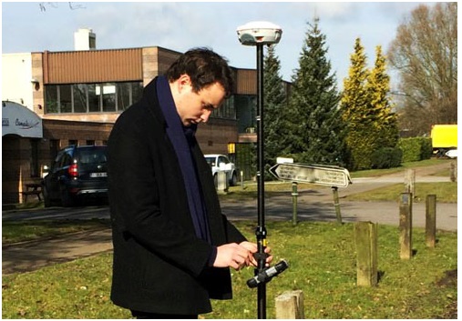
Experiencing the Qiao Station with ComNav T300 for surveying.
Europe’s first commercial BeiDou CORS station — Qiao CORS Station — has been built in Wallonia, Belgium. ComNav partnered with local company CGEOS – Creative Geosensing on the project. ComNav develops and manufactures GNSS OEM boards and receivers for demanding high-precision positioning applications.
Qiao means bridge in Chinese, and Joël van Cranenbroeck, managing director of CGEOS, is working to build the bridge between the Chinese and European GNSS industries by introducing the Chinese high-precision GNSS technologies of ComNav Technology to European users, ComNav said in a statement.
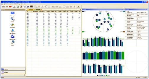
The Qiao Station can track BeiDou Navigation Satellite System on the three frequencies and transmit observation data in RTCM format in real time through NTRIP and observation data in RINEX format. It enhances the positioning performance and result by combining BeiDou with GPS and GLONASS.
Currently, the BeiDou Navigation Satellite System mainly covers the Asia Pacific region. Though China is still in the process of building it into a global network, up to six BeiDou satellites can now be tracked in Europe during certain periods of the day. With the new Qiao Station, European users can now try the BeiDou system.
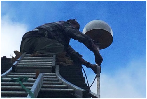
Setting up Qiao Station.
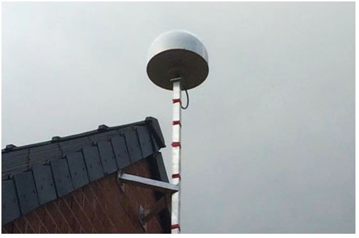
European’s first BeiDou CORS station has been built in Belgium.
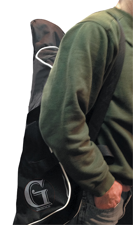
Geomatics USA from Gainesville, Fla., has designed a precision surveying and mapping system that can be easily stowed in an overhead compartment for airline travel. Surveyors can fit everything needed for important mapping and surveying jobs into a baseball-style bag, including tripods. The compact, light-weight system offers differential sub-foot accuracy.
Components easily pack into a baseball-style case.
The G1-m1 receiver system has many advantages over conventional GNSS receivers, Geomatics said. The system is designed for precision surveying jobs that require travel to remote areas of the world, and for traveling to job sites by commercial airline. The complete base and rover kit, including the tripods, rods, and batteries, fits into a single baseball style bag and weigh less than 10 kg, making it easy to stow as carry-on luggage.
The Geomatics USA G1 system is scalable from a simple single-frequency semi-mobile receiver — ideal for control networks and some semi-kinematic mapping applications — to a dual-frequency network RTK solution. All of the Geomatics USA G1 solutions perform precision-quality tasks at a fraction of the cost of major-brand equipment.
The G1-m1 system comes with a free processing software license for the first 50 systems that supports carrier-phase relative positioning and CA-code differential correction. The software is designed with a simple user interface for easy selection of base and rover data or automatic data download of the closest Continuously Operating Reference Station (CORS) from the U.S. National Geodetic Survey database. It is compatible with other RINEX based post-process systems around the world.
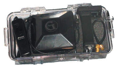
Complete survey set including GNSS receiver, antenna, battery and cables, fits in a small handheld plastic case.
According to Geomatics USA Chief Technology Officer Ahmed Mohamed, “The G1 product line fills the gap between survey applications, where cm-level precision is an absolute necessity, and mapping applications, where meter-level precision is acceptable. In fact, the G1-m1 product offers sub-foot precision in most cases and cm-level precision in ideal situations. Geomatics USA uses readily available components and open-source code to develop its end user product solutions. The objective is to make sure the software performs correctly with a very short learning curve for the user.”
For a limited time, Geomatics is offering a specially priced configuration for the first 50 systems through NavtechGPS, its worldwide distributor.
Being a person who enjoys spending time in the field using RTK and DGPS, I followed up on my column last month, “Sources of Public, Real-time, High-Precision Corrections,” with a trip to the field to test the NGS CORS Streaming service. About a month ago, I made a trip to Colorado to attend the Space Weather Workshop in Boulder, stop by the SPAR conference in Colorado Springs, and visit with some of my colleagues in the Denver area.
When I arrived in Denver, my plan was to meet Tim Smith (GPS Coordinator for the U.S. National Park Service) and travel to the Bakerville GPS test site in the Rocky Mountains, which was at about ~11,000 feet in elevation. My intent was to test the CORS Streaming and PBO real-time streaming that I discussed last month to better understand the accuracy and reliability of those services.
I arrived at the Denver airport early on a Monday ready to rock and roll into the Rockies with some high-precision GNSS equipment. As it turned out, I was denied. In Colorado, the weather is dynamic. It was quickly degrading when I arrived in Denver. Snow was definitely in my future for the next few days. Tim made the decision that we shouldn’t travel to Bakerville. The reason for Tim’s trepidation wasn’t necessarily due to the weather in Bakerville, but rather that the I-70 Interstate might turn into a parking lot and we’d be stuck in traffic for a few hours. Fair enough. The backup plan was to do some local testing in the parking lot adjacent to Tim’s office in Denver.
Tim invited Mel Philbrook to join us. Mel is a long-time GNSS technologist who works for the local Trimble dealer. He brought an SUV full of Trimble GNSS equipment, including one of the new R10 GNSS units as well as a GeoXH handheld with an external antenna.
Mel also had an Intuicom RTK Bridge in the trunk of his SUV that facilitated the different sources of RTK reference data we could use. He could switch from CORS Streaming to the local VRS via NTRIP to UHF at the flip of a switch, sending corrections to both the R10 and the GeoXH. I was particularly interested in seeing how the units performed using CORS Streaming, which is/was a free RTK service (single baseline) that was in beta test phase. In Oregon, I don’t have access to CORS Streaming because the only CORS Streaming station west of the Mississippi River is in Boulder, Colorado. The station is TMGO (Table Mountain CORS).
The baseline distance from TMGO to our location was about 55 km. The R10 was reporting a horizontal precision of about 4 cm. Not bad for a 55-km baseline. I didn’t compare the results to a survey mark (shame on me, but keep reading because I get to that) so I’m trusting the R10’s precision estimate. Tim said he’s run the test before using a GeoXH and a longer baseline and saw sub 10-cm horizontal precision. It’s not what the typical person using short baseline or RTK network is accustomed to, but for the high-precision GIS user who’s mapping utility, transportation, and infrastructure, that’s pretty darn good.
Tim, Mel and I spent an hour or so messing around with the equipment before packing it up. Not a very scientific study, but it confirmed that CORS Streaming was accessible via NTRIP and reasonably accurate.
In the meantime, the snow wasn’t letting up. This is the view as I was leaving Tim’s office to head to Boulder for the Space Weather Workshop:
I wasn’t finished with my CORS Streaming testing yet. My experience at Tim’s office gave me enough confidence to allocate time later in the week to conduct a more detailed test after the Space Weather Workshop. Hopefully, the weather would cooperate (call me a fair-weather field guy).
Space Weather Workshop
Every April, NOAA’s Space Weather Prediction Center in Boulder hosts the Space Weather Workshop (SWW), a gathering that has evolved into the leading conference in the U.S. for space weather-related topics. It attracts attendees, experts and speakers from all over the world. The discussion isn’t centered on GNSS, but GNSS certainly is a topic that is discussed. This year’s central topic was the electric power grid. You can view the SWW program here.
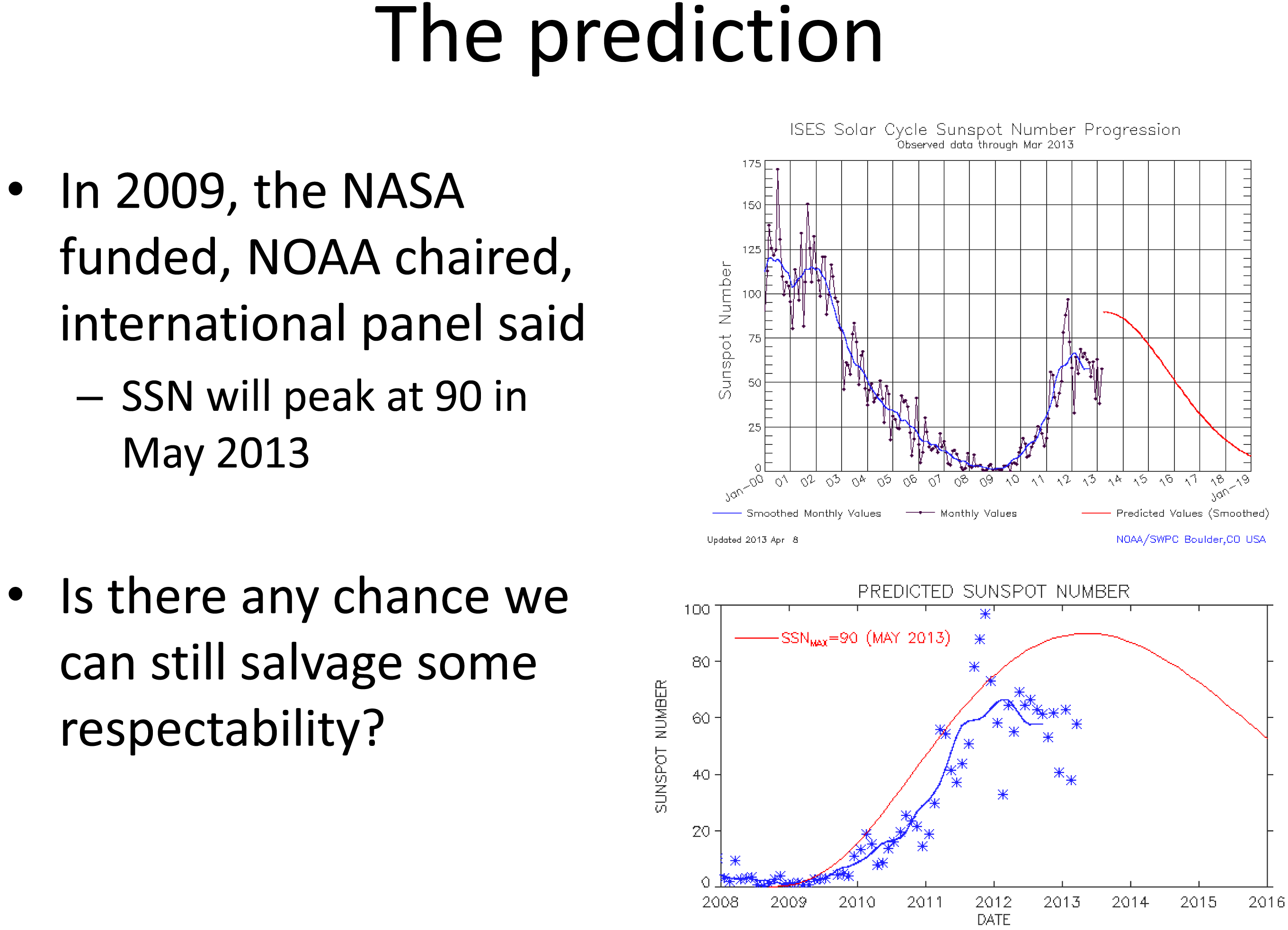
Believe it or not, this month (May 2013) was the predicted “solar maximum” for the current solar cycle (Solar Cycle 24, an 11-year cycle). However, Solar Cycle 24 has been unexpectedly weak. See the following slide presented by Doug Bisecker of the Space Weather Prediction Center. Doug is the Chairman of the Solar Cycle 24 Prediction Panel. His question, “Is there any chance we can still salvage some respectability?” speaks volumes about the difficulty in predicting space weather.
Source: Doug Bisecker presentation at the 2013 Space Weather Workshop
From the above, you can see the actual number of sun spot occurrence has been significantly less than predicted. Although sun spots aren’t what cause GNSS receivers to have problems, sun spots can indicate the amount of solar activity, which can be related to geomagnetic storms. Geomagnetic storms disturb the ionosphere and are the events that cause the most problems for GNSS receivers. Looking at the top chart above, you can see the difference in activity between the last solar maximum (peaked in early 2002) and today. The difference is clearly significant.
Does this mean we, the high-precision GNSS users, get a free pass on Solar Cycle 24?
Not at all.
Historically speaking, the most extreme geomagnetic storms (e.g., Oct/Nov 2002) have occurred after the solar maximum so our sensitivity to this issue should be keen for the next two years. Furthermore, there are orders of magnitude more high-precision GNSS receivers being used than ever before, and in mission-critical applications such as auto-steer in machine control (agriculture, construction, etc.). Most GNSS high-precision users today haven’t experienced the effects of an extreme geomagnetic storm. For a short primer on the effects of solar activity on GNSS/GPS, you might want to take a look at this article I wrote in 2008 as well Richard Langley’s 2011 Innovation column “GNSS and the Ionosphere.” In addition to the content, they both contain some valuable links to relevant articles.
In line with a goal of the workshop, a panel of GNSS professionals looked at issues that users face as they go about their business at solar max. The panel was “Global Navigation Satellite System (GNSS) Services: Research Needed to Fill Operational Gaps.” Joe Kunches (SWPC) moderated the panel that included Dr. Geoff Crowley (Astra), Dr. Anthea Coster (MIT), Capt. Steven Miller (USAF) and myself. We highlighted precision GNSS, satellite navigation for commercial aviation (ADS-B), and current work to better understand the errors the ionosphere imposes on user activities.
Something else I learned at the conference was how tough ionospheric scintillation is on GNSS receivers in Brazil. I feel for those users. When I mentioned I was traveling to Chile for an RTK project, the scientists said it is worse in Chile than the U.S., but still not as bad as Brazil. I’ll be very interested to experience how different it is than the U.S. (or other parts of the world where I’ve traveled).
I keep a pretty close eye on space weather and in contact with NOAA’s Space Weather Prediction Center. When I hear of a space weather event that may affect high-precision GNSS/GPS receivers, I send out a Tweet with the hashtag #SolarActivity. You can follow me on Twitter at https://twitter.com/GPSGIS_Eric.
From Space Weather Back to Local Weather
As the week progressed during the Space Weather Workshop, the snow continued. Boulder looked like Christmas in April.
I really wanted to spend some more time in the field to test the accuracy of the NGS’s CORS Streaming service and I was running out of time. In order to perform the test the way I wanted, I needed to find a local NGS survey mark that was observed using GPS. I checked out the NGS survey mark database and got lucky. There was one (PID = KK2060) located on a vista point parking area off of Highway 36 on the way from my hotel to the Space Weather Workshop. I couldn’t have asked for a better or more convenient survey mark location. I was planning to use a Bluetooth GNSS receiver so I could actually collect data while sitting in my car.
On Thursday morning, Mother Nature cleared her skies for me so I drove to the vista point. Remember, there’s a couple of feet of snow on the ground, so I was really hoping to see some kind of wood lathe that would get me close to the survey mark (no, I didn’t preload the KK2060 coords in my GPS L). Fortunately, a wood stake was near the survey mark. However, I didn’t have a shovel or a metal detector so it was either using my hands to shovel and search under two feet of snow for the mark, or…thanks to the rental car company, the car came with a healthy-sized windshield scraper. After 15 minutes of digging in the snow with a windshield scraper, I found KK2060. I’m sure to the people parked on the vista enjoying the view; I looked very suspicious using a windshield scraper to dig a hole in the snow. I wouldn’t have been surprised if a state trooper had shown up.
KK2060 recovered from under two feet of snow with a windshield scraper.
My final challenge was…no tripod or tribrach. I travel light and didn’t want to pack a set and, of course, I forgot to ask Tim if I could borrow a set. It’s never a good idea to set a GNSS antenna directly on the ground, but the antenna was small (<3” in diameter) and I did have a 5” diameter ground plane with about a 1” post. I was able to place it over the survey mark with reasonable confidence.
As I mentioned before, I was using a Bluetooth GNSS receiver (GPS L1/L2, GLONASS), the SXBlue III GNSS.
To collect the data, I was using an SXPad handheld with an AT&T SIM card for the Internet connection. For data-collection software, I used VisualGPSce, a free GPS data-collection program that collects and displays raw NMEA data. Although it doesn’t display enough digits of precision for the horizontal position, it accomplishes the simple task of collecting NMEA-formatted data without applying any transformation so I get the raw NMEA-formatted data from the receiver. It also displays some useful information such as PDOP, RTK indicator and elevation.
The last piece of data-collection software I used was a free NTRIP client software written by the SXBlue people called SXBlue RTN. I needed an NTRIP client software to access the CORS Streaming mount point. The software manages the IP address, port and login/pwd of the CORS Streaming system.
Logging into the NGS CORS Streaming site was painless, and within a few seconds I had an RTK FIXed position from the GNSS receiver, all from the comfort of my rental car, thanks to long-range Bluetooth. I collected ~45 minutes of NMEA data (1-Hz data rate) without interruption.
When I returned to the office, I began the process of comparing the results from CORS Streaming to the NGS survey mark coordinate. I checked with NGS and they reported that CORS Streaming is referenced to the ITRF00 (epoch 1997.0) datum. The KK2060 coordinate is published in NAD83/2011 (epoch 2010.0). I needed to reconcile the datum difference before performing any analysis so I used the NGS HTDP (Horizontal Time Dependent Positioning) online tool to accomplish this.
Finally, I used NMEA Analyzer (custom-built software for performing statistical analysis on GNSS NMEA data to NSSDA horizontal accuracy standards) to calculate accuracy (not precision) values of the data. I set up the NMEA Analyzer software to randomly select 200 epochs out of the ~2,700 collected to mitigate any bias due to filtering or other receiver “tricks”. Following are the horizontal results:
Not bad for an antenna sitting on the ground and an 18-km baseline using a $6,000 GNSS receiver and a free RTK base station. Folks, this is the direction that GNSS technology is heading. The continued proliferation of high-precision GNSS infrastructure (RTK networks, real-time PPP, etc.) and the falling prices of RTK GNSS receivers will dramatically increase the availability of high-precision technology to those who previously could not afford to make the investment.
I didn’t get a chance to test the PBO real-time streaming while I was in Colorado, but fortunately there are many PBO real-time stations that I can test from the comfort of my home office here in Oregon. In fact, there are so many in Oregon and Washington that I can test many different baseline distances to understand what accuracy users can expect. Look for my test results on that sometime this summer.
National Geodetic Survey (NGS) Suffering
Only a week after I did my field test of NGS’ CORS Streaming system in Colorado, NGS announced it was shutting down the CORS Streaming service effective April 26. On April 23, NGS issued the following notice by email:
*********************************************
The National Geodetic Survey’s prototype Real Time GNSS Data Service (Streaming CORS) will be discontinued effective April 26, 2013. The prototype was introduced a few years ago as a small research project to gauge interest and usage as well as test a proof of concept with the RTCM communities. However, due to low usage of this prototype service and staff limitations within the National Geodetic Survey, we have decided to discontinue the prototype. There were many contributing factors that lead to this decision but the following recent series of events has had a significant impact on project support and operations:
— Funds were cut due to sequestration and rescission
— Upcoming furloughs will impact all National Geodetic Survey Personnel
— A NOAA-wide hiring freeze is in effect
— Our only real-time expert will retire on April 30, 2013
If you have any questions or comments to share, please contact Neil Weston at 301-713-3191 or by email – [email protected].
*********************************************
I think the action was premature. Hardly anyone knew about the CORS Streaming service and it was only deployed in a small number of locations, which was not enough to cover a significant geographic area or major metro areas.
Nonetheless, I think this action points to bigger problems at the NGS. To all of us in the U.S. (and those in other countries), the NGS has been a tremendous source of GNSS technical expertise, products and services. The problem is that they are losing expertise at a faster rate than they are gaining. Just in the past few months, Dave Doyle and Bill Henning have both retired. Those two were a big part of the NGS user community outreach “boots on the ground” effort.
Furthermore, as the notice indicates, NGS’s only “real-time expert” (Bill Henning) is now retired. That’s a problem. As real-time, high-precision GNSS is gaining traction quickly in industries beyond surveying and engineering, the resources for NGS to support this trend should also expand, not contract. On the other hand, the use of GNSS post-processing is not increasing, yet NGS has loads of resources allocated to support post-processing. As technology trends shift, resources need to be redistributed in alignment with those trends.
The Future of NDGPS Open for Public Comment
The U.S. NDGPS program is on the chopping block again. However, this time it’s much more serious. The last time this issue surface was in 2007 when funding for some of the NDGPS sites was being threatened. At that time, only some of the inland sites were facing decommissioning. The U.S. Coast Guard DGPS part of NDGPS was safe and funded.
However, that’s not the case this time. Even the U.S. Coast Guard is starting to question the value of the DGPS system it created and has been using for more than 15 years. The FAA’s WAAS (Wide Area Augmentation System) has proven to be a viable alternative to NDGPS and is used by thousands of sport mariners and commercial marine pilot associations across the U.S., as well as high-precision users in GIS and surveying/engineering. To further complicate the issue, the use of GLONASS is not supported by NDGPS. Like what we’ve seen in high-precision surveying/engineering receivers, GLONASS is becoming an important feature in receivers used by commercial mariners who have to deal with terrain and structures that impede satellite visibility. Even though WAAS doesn’t support GLONASS, some newer GNSS receivers are able to integrate GLONASS data into the WAAS solution, further increasing the value of WAAS over NDGPS.
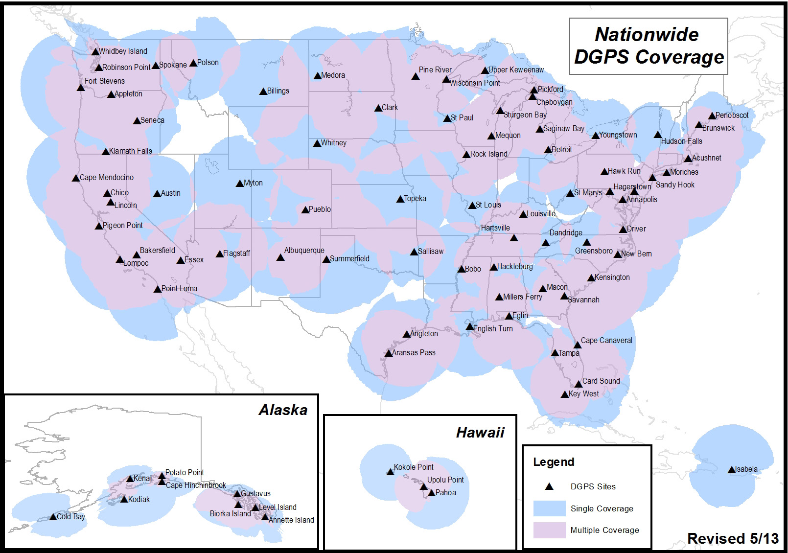
It’s likely that you aren’t an NDGPS user, but you might still be affected if the NDGPS is decommissioned. There are a total of 86 NDGPS stations across the Continental U.S., Alaska and Hawaii. As well as being NDGPS signal broadcasters, they are also part of the NGS CORS program that is used by the NGS’s OPUS online post-processing service. If you are using OPUS or NGS CORS for post-processing, you might be using NDGPS CORS data and not realize it. Following is a map of all NDGPS stations in the U.S.:
U.S. NDGPS coverage map.
If you’re interested in reading an explanation from the U.S. Coast Guard and Department of Transportation about the request for public comment and submitting a comment, click here. To be considered, comments must be submitted by July 15.
The team installs a HARNS in the southern province of Basra. Since 2005, Iraqi engineers have attempted to recover HARNS, but many were destroyed by locals who thought they indicated buried treasure.
As a geodetic surveyor, I served in the U.S Army for 10 years. During that time, my team and I developed a nationwide GPS infrastructure system called the Iraqi Geospatial Reference System (IGRS). We installed Continuously Operating Reference Stations (CORS) and High Accuracy Reference Network Stations (HARNS), the first Iraqi owned and maintained system of its type.
As a native Arabic speaker, my role was to train the Iraqi engineers to install additional CORS, as well as update and maintain the IGRS as a part of the International GNSS Service (IGS) network to sustain the accuracy of engineering and mapping projects. The IGRS was critical to other major infrastructure projects in the effort of rebuilding the battered nation, such as telecommunications, public works, and natural resource management to name a few.
Some of the CORS we installed have Virtual Reference System (VRS) capability, a technology newly developed to establish real-time corrections in the field by using CORS as a base station for real-time kinematic (RTK) data collection.
Key coordinators for the installation included Wisam Al-Hassani of the Iraq Ministry of Water Resources, Paul McKenzie of the Canadian Army, Linda Allen of the U.S. State Department, and myself, representing the U.S. Army, in addition to representatives from National Geodetic Survey (NGS), National Geospatial-Intelligence Agency (NGA), and Trimble Navigation.
In addition to developing the IGRS, we performed several critical projects to assist in the rebuilding efforts as well as providing force protection, navigation, and mapping. My topographic engineering unit was responsible for providing coalition forces with GIS analysis, map production, and geodetic surveys.
GPS equipment collecting data on a reference benchmark used to monitor the deformation of the Haditha Dam.
For my second tour in Iraq (2007–2008), I was the platoon sergeant, which is equivalent to a project manager in a surveying firm. During the 15-month deployment, my team performed various survey projects including: 10 airport obstruction surveys, a dam deformation survey, more than 30 artillery and target-acquisition radar surveys, base-camp designs, site layouts, and ground-truth data collection for photogrammetry and remote sensing projects. We also established a nationwide database of all survey control stations in Iraq. The CORS was installed using Trimble NetRS receivers and Zephyr geodetic antennas. Trimble GPSNet and GPSBase software were used to process the continuous satellite data, for inclusion in the worldwide CORS network for public use. Field survey operations were conducted using Trimble 5700 GPS equipment.
Traveling in Iraq was a major obstacle for survey operations. We had a choice: either fly on helicopters or drive military vehicles. Flying in helicopters with survey equipment was a challenge because we could never fit all our personnel and equipment. However, it was much safer than ground transportation through the dangerous roads of Iraq. In one incident, we were building a bridge in Baiji to help Iraqis and coalition forces cross the Tigris River after the original bridge was destroyed during the 2003 invasion. Our vehicle hit an improvised explosive device (IED). Some of the survey equipment was damaged, but we went back the next day and eventually built the bridge.
Anas Malkawi served 10 years in the Army as a geodetic surveyor and senior technical engineer. He is currently enrolled in Old Dominion University’s Civil Engineering program while working at Transocean International Corporation as the Iraq program manager.
The initial plan of IGRS and placement of CORS/HARN through the Southern provinces.Soldiers establish geodetic control for an airport aeronautical survey.Soldiers survey airport navigational aids that require high geodetic accuracy.Malkawi discusses installation of Iraqi operated and maintained CORS with Al-Hassani.The result of traveling in military vehicles over roads infested with IED.Key coordinators for the installation of the first Iraqi owned and maintained Continuously Operating Reference Station (CORS.) From left are Hussein, Malkawi, McKenzie, and Allen.The 2005 U.S./British IGRS Team. Despite the difficulties, the soldiers I am honored to have served with stayed motivated and performed exceptionally every day by providing accurate data that saved lives.
The use of a precise wide-area positioning technique for airborne trajectory solutions for LiDAR surveys provides both relative and absolute accuracies similar to those derived from using a local GNSS reference station.
Airborne light detection and ranging (LiDAR) surveys are among the most advanced means of producing high-resolution, accurate surface elevation models used for many applications in surveying and civil engineering. Precise geolocation and orientation (or georeferencing) of the LiDAR instrument with a combination of on-board GNSS and inertial sensors at the times when the measurements are made provides the key to high-quality elevation products.
The usual practice deploys reference GPS/GNSS land receivers in the area where the aircraft will be flying, to obtain a precise trajectory by short-baseline differential GNSS techniques. This could mean installing and operating receivers at many sites during a flight mission if the area surveyed is a large one.
We have tried a different approach: using as reference receivers those of a sparse network of Continuously Operating Reference Stations (CORS) in New South Wales known as CORSnet-NSW, and a wide-area differential GPS technique for obtaining the aircraft trajectory with sub-decimeter accuracy even with baseline lengths of several hundred kilometers. This may be comparable in precision and accuracy to the short-baseline method, but without the cost and logistical complications. This opens up a new level of operational capability, allowing flexibility for weather conditions and priority response applications.
The tests described here were organized and conducted by the NSW government’s Land and Property Management Authority, in collaboration with the University of New South Wales, in June 2009. CORSnet-NSW consists, at this writing, of 46 stations and by 2012 will provide statewide GNSS positioning infrastructure across NSW with a planned 70 stations in operation.
Precise Wide-Area Positioning
We used a technique for long-baseline differential, off-line positioning, able to deliver centimeter precision for fixed receivers and sub-decimeter precision for moving receivers. This choice was dictated by three considerations:
The intended application was the geolocation of the data of an airborne scanning LiDAR sensor to be used in the generation of high-accuracy digital elevation models (DEM).
Off-line processing, where all the GNSS data collected during the flight are available for processing and (as in this case) there is no need for immediate results, is intrinsically more reliable than real-time processing, where the data are available only up to the present epoch, and accurate results must be obtained right away, with no chance for a second try.
Differential processing makes it possible to resolve the carrier-phase ambiguities using well-understood methods.
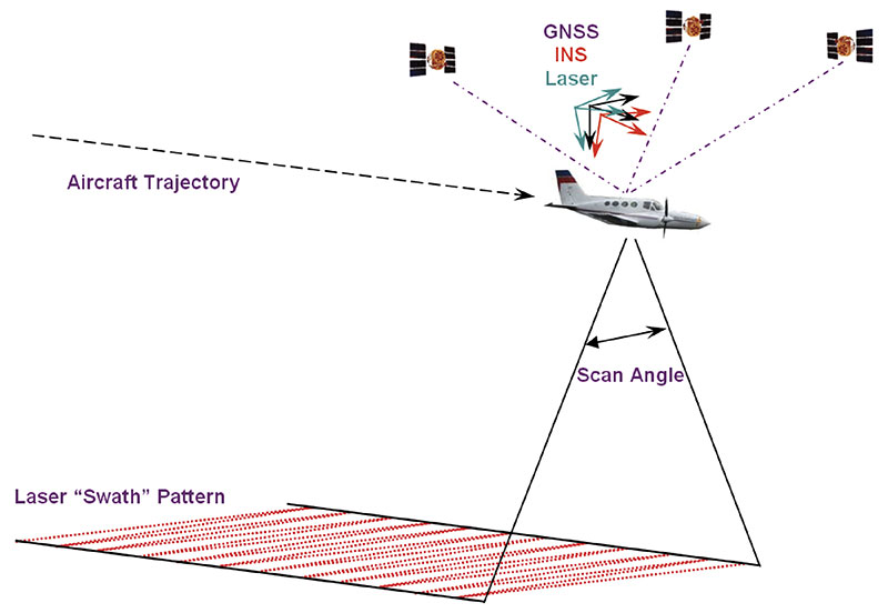
Technique. It is common practice in airborne LiDAR surveys to use GNSS both to position the instrument precisely, and to assist an inertial navigation system (INS) to obtain the orientation of the aircraft in space, as both position and orientation are needed to interpret the data properly. FIGURE 1 illustrates the relationship between the sensors used for airborne LiDAR surveys. The aircraft uses a GNSS antenna combined with an INS to georeference its trajectory. The bore-sight calibration process aligns the individual sensor orientations and standardizes the range measurements. However, if the survey is to achieve the now-expected high level of vertical accuracy (615 centimeters, 1 sigma), then the position of the GNSS/INS-derived aircraft trajectory for each laser swath must be determined with a relative precision in the order of just a few centimeters. This is achieved via differential GNSS post-processing of the kinematic airborne data together with static observations collected on precisely surveyed ground reference stations. The GNSS positions are then blended with high-frequency measurements taken by the onboard INS to produce the final trajectory and reference orientations.
Figure 1. Airborne LiDAR reference frame.
To such ends, the aircraft trajectory is usually determined by short-baseline differential GNSS, with ground receivers deployed near the intended flight path of the aircraft. In this way it is possible to use GNSS data analysis techniques that are both precise and quite straightforward to implement in software. The simplicity of these techniques is possible because, in short-baseline differential solutions, the data of the aircraft receiver and any nearby network receivers have much the same systematic errors (due to such things as satellite ephemerides errors, transmission delays, and so on) that cancel out — or nearly so — when their observations are differenced between them. This also makes it possible to resolve quickly and reliably the cycle ambiguities in the observed carrier phase, the most precise type of GNSS data, overcoming one of the main obstacles to obtaining good results. Furthermore, it is possible to get such results with single-frequency receivers, as ionospheric delay is one of the systematic effects that can be largely canceled out.
In wide-area solutions, those cancellations are not complete enough to ignore the systematic data errors, and they have to be included in the form of additional unknown parameters in the observation equations. Also, it is necessary to account for the ionospheric delays using dual-frequency data, which means using more expensive GNSS receivers and antennas.
Resolving the carrier-phase ambiguities is no longer straightforward or assured. The standard way of dealing with the ambiguities is to include them as unknowns in the observation equations and adjust them along with the other unknowns: this is often referred to as “floating the ambiguities.” Fixing (or resolving) those ambiguities to their most likely integer values in a matter of seconds to a minute is possible on occasion, when the aircraft is within less than 20 kilometers from a ground receiver, or very precise corrections for the ionospheric delay are available; otherwise slower techniques, that require tens of minutes, may be used. It is also necessary to correct as well as possible such things as the neutral atmospheric delay of the GNSS radio signals, the movement of the “fixed” stations due to plate tectonics, the solid earth tide using mathematical models, and, in the case of the tropospheric delay, estimating the error in the corrections made using a standard formula as an additional unknown per receiver.
Over the years all these difficulties have been gradually dealt with more effectively, more efficiently, more reliably and, from the user’s point of view, less painfully. Originally developed for the repeated determination of station positions to measure the slow tectonic deformations of the Earth’s crust, and to calculate precisely the orbit of Earth-observing satellites, these days, after nearly 30 years of steady progress, GNSS wide-area techniques and the corresponding software find many applications in science, engineering, and navigation, and are becoming widely used in remote sensing.
Software. We used the Interferometric Translocation (IT) wide-area positioning software developed by one of us for the long-baseline aircraft trajectory solutions and also to re-position in the IGS05 international reference frame some CORSnet-NSW stations, so their data could be used consistently in the differential wide-area solutions. These stations were originally given in the Geocentric Datum of Australia (GDA94). For both purposes we used the precise final GPS orbits computed and distributed by the IGS.
To validate the aircraft trajectories calculated with the wide-area method, we relied mainly on the quality of the LiDAR DEM results obtained with those trajectories. We also used commercial software to generate short-baseline differential solutions with receivers deployed near the intended aircraft flight-path, as is common practice in this type of survey, and compared them with the wide-area solutions (they turned out to be quite similar to short-baseline solutions obtained with the wide-area software).
Airborne Tests
This study has used data from two airborne LiDAR surveys conducted by the NSW Land and Property Management Authority (LPMA) in June 2009. The first took place near the township of Glen Innes, and the second was a bore-sight calibration flight near the city of Bathurst. For both LiDAR surveys, the following data were acquired:
Aircraft trajectory, raw dual-frequency GPS (1 Hz) and IMU data (200 Hz).
LiDAR (raw return data for each laser pulse).
GPS reference station data from local receivers and multiple CORSnet-NSW sites.
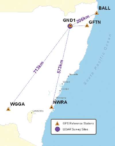
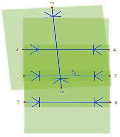
Glen Innes Test. This operational LiDAR survey established GND1 as the local reference station within the survey area. CORSnet-NSW data were collected for the test from GNSS receivers in Ballina (BALL), Grafton (GFTN), Nowra (NWRA), and Wagga Wagga (WGGA). FIGURE 2 shows the distribution of the reference stations and the flight runs.
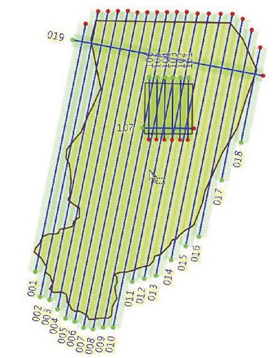
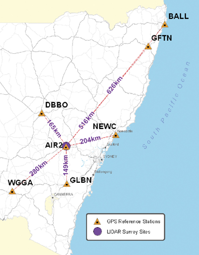
Figure 2. Glen Innes survey of June 9, 2009, showing the distribution of reference stations with baseline lengths and the survey area with (numbered) flight runs.Bathurst Test. Bathurst Airport is LPMA’s LiDAR calibration site and has various arrays of accurate ground checkpoints. AIR2, near the runway of the Bathurst airport, is the locally established GNSS reference station. CORSnet-NSW data were collected for the test from receivers in Ballina (BALL), Dubbo (DBBO), Grafton (GFTN), Newcastle (NEWC), Nowra (NWRA), and Wagga Wagga (WGGA). FIGURE 3 shows reference-station distribution and a schematic of the flight runs.
Figure 3. Bathurst test of June 16, 2009, showing the distribution of reference stations with baseline lengths and the survey area with (numbered) flight runs.
Effect on LiDAR Data
Rather than simply comparing aircraft trajectories, this study aimed to determine what effect the use of wide-area GNSS positioning has on the actual LiDAR point data and associated elevation surfaces. In terms of the horizontal accuracy required for LiDAR surveys, initial tests showed that the differences between the horizontal positions of various trajectories was negligible; therefore, only the vertical component was considered in this analysis.
To quantify differences between LiDAR data generated from trajectories using various combinations of distant GNSS reference sites, we applied four types of analysis:
Comparison of trajectories — directly compare the locally computed trajectory (assumed to be truth) with each wide-area derived trajectory.
Relative LiDAR point comparison — compare the positions for a sample of LiDAR ground points derived from the locally computed trajectory with those derived from each wide-area derived trajectory.
DEM comparison — difference the raster surfaces derived from the locally computed trajectory and a wide-area derived trajectory to find the effect over a LiDAR run.
Absolute LiDAR ground control comparison — compare the LiDAR derived surface from various trajectories to the surveyed ground control (Bathurst Calibration test site only). This also involves vertically shifting the resulting surface so that its offset relative to the one used as control is zero, thus removing the effect of using different reference frames for the GNSS trajectories and the control surface.
Trajectory Comparison
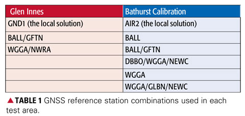
The comparison between the locally determined and each wide-area derived trajectory was made along the entire trajectory for each flight. The importance of this step lies in the assumption that all LiDAR data are directly positioned from the trajectory and so any systematic effect in the trajectory should be reflected on the ground. For each test site the locally derived solution is assumed to be “truth” with the vertical difference computed against wide-area solutions for each combination of reference stations used (TABLE 1).
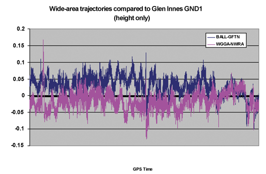
Glen Innes Test. FIGURE 4 shows the vertical comparison of two wide-area derived trajectories (using BALL and GFTN, and WGGA and NWRA, respectively) against the locally derived trajectory (using GND1). It can be seen that once the aircraft attained its stable operating altitude, the wide-area derived trajectories are generally within 5 centimeters of the locally derived solution.
Figure 4. Trajectory elevation differences for entire Glen Innes flight.
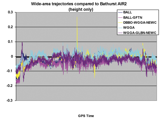
Bathurst Test. The Bathurst test differs from the Glen Innes test in that both the duration of the flight and the length of each run are significantly shorter. FIGURE 5 shows the vertical component of five wide-area derived trajectories, using several combinations of CORSnet-NSW reference stations, compared against the locally derived trajectory (using AIR2). The results once again show a remarkably consistent comparison with the locally derived solution. Data spikes showing up in the DBBO/WGGA/NEWC (yellow) solution were attributed to small data glitches at the DBBO CORSnet-NSW site. Unfortunately, LiDAR data were not collected at those instances; therefore, the effect on ground data could not be fully assessed.
Figure 5. Trajectory elevation differences for entire Bathurst calibration flight.
Relative Comparison
Regardless of the trajectory and orientation used to georeference LiDAR data, the same number of points will be created. It is therefore possible to create a LiDAR dataset using the same raw LiDAR data but different GNSS trajectories, and compare the results to determine the relative positioning differences on the ground.
Given the large number (many millions) of points in a LiDAR dataset, we used a representative sample of evenly spaced 10 2 10 meter areas each containing 50–100 points (on level ground) for statistical analysis. We calculated displacement vectors between points computed from the locally derived trajectory and those using wide-area trajectories. Results from flight run 002 at Glen Innes (see Figure 2) and run 7 at the Bathurst Calibration test site (see Figure 3) are presented here.
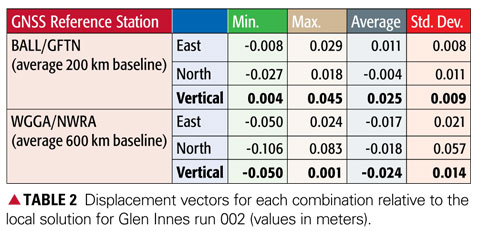
Glen Innes Test Run 002. The displacement vectors from 46 sample areas (4,620 points) are summarized in TABLE 2, being points computed using the two wide-area solutions compared with the locally derived solution using reference station GND1. Note the high accuracy achieved in the all important vertical component.
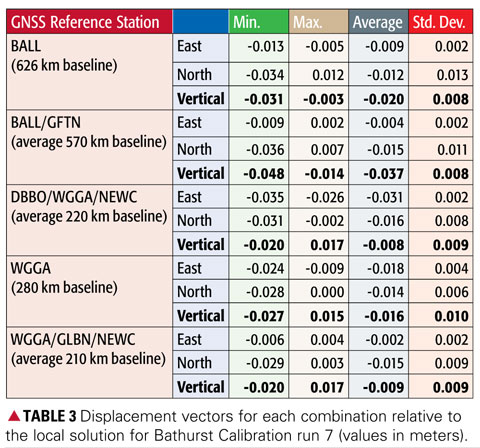
Bathurst Test Run 7. The displacement vectors from 25 sample areas (1,700 points) are summarized in TABLE 3, being points computed using the five wide-area solutions compared with the locally derived solution using reference station AIR2. Once again the results clearly show that the height values agree to within a few centimeters, even over baselines of more than 600 kilometers in length.
DEM Comparison
To investigate how the LiDAR surfaces derived from each trajectory compare across the entire data swath, we created raster surfaces from the LiDAR point data. Each surface was then subtracted from the local solution to create a difference surface. Visual inspection and interpretation was then used to discern any patterns or effects.
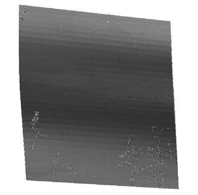
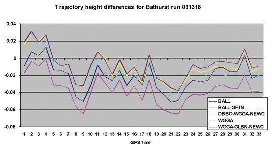
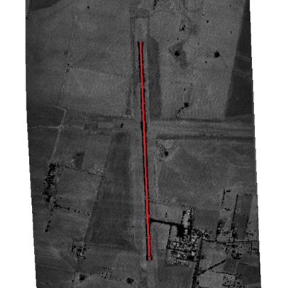
The result shown in FIGURE 6 (Bathurst Calibration flight run 7) was typical of the cyclical effect evident for all solutions. The magnitude of the difference was in the order of 2–3 centimeters and is in the direction of flight (north to south). If this cyclical variation is compared with the trajectory comparison for just the 33-second duration of flight run 7, a clear (expected) correlation with the variation in height is evident (FIGURE 7).
Figure 6. Subtraction surface for Bathurst Calibration run 7 (AIR2 vs. BALL).Figure 7. Trajectory comparison for Bathurst Calibration run 7 (031318).
No DEM comparison results are presented for the Glen Innes data because of significant variation in terrain and vegetation, making interpolation difficult and unreliable.
Absolute LiDAR Comparison
Ground control points serve two purposes in a LiDAR survey:
The calculation of statistics to describe vertical accuracy, that is, quantifying the match of the surface to the local height datum.
The calculation of a surface adjustment to enable transformation of the LiDAR points to fit the local height datum.
Additionally, ground control points with accurate heights are used to calibrate the sensor before use in active LiDAR surveys to account for internal electrical delays in the ranging and measurement system. LPMA maintains a calibration site at Bathurst Airport for this purpose, and regularly surveys the area to ensure the sensor is operating at maximum accuracy. It should be noted that the sensor was calibrated using Bathurst Airport ground control data prior to this study.
Surveyed Ground Control. The airport runway centerline vertical profile for the Bathurst Calibration site (FIGURE 8) was re-computed in terms of the same IGS05 reference frame determined for the LiDAR trajectories, thereby allowing an independent comparison with ground truth.
Figure 8. Runway vertical profile at the Bathurst Airport calibration site.
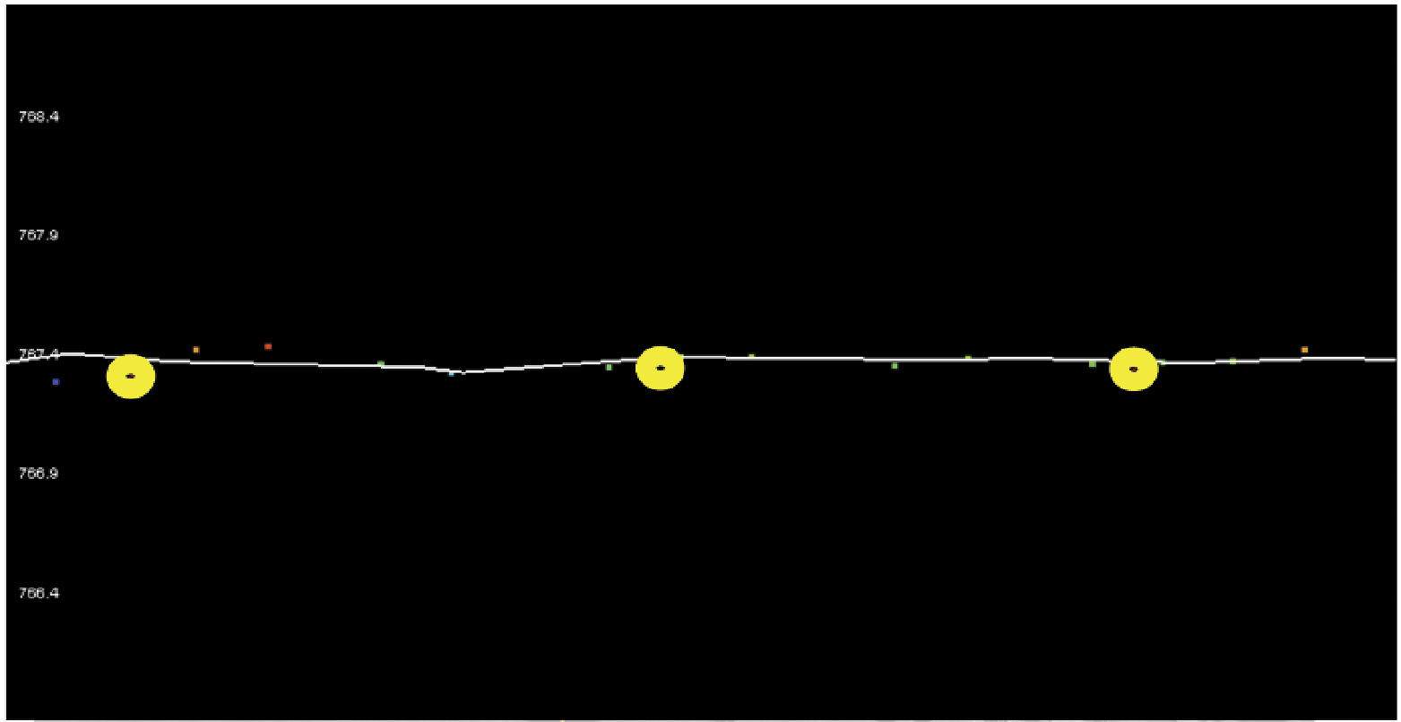
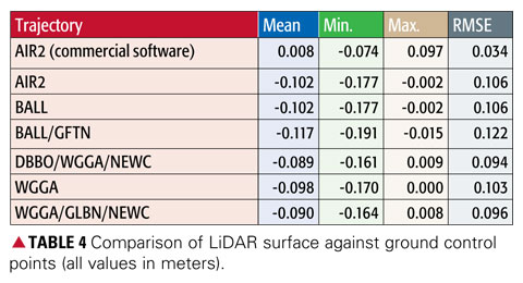
Point Comparison. Data from Bathurst run 7 were used to compare LiDAR results with the established ground control using a basic triangulated irregular network (TIN) surface comparison (FIGURE 9 and TABLE 4). In Figure 9, the TIN surface is indicated by the white line, while the ground control points are shown with yellow buffers.
Figure 9. Comparison of LiDAR surface and ground control points.
The first trajectory in Table 4 is the original calibration comparison using commercial software and orthometric height data. All wide-area solutions display a similar vertical offset, because of the use of different reference frames for the GrafNav and wide-area solutions (IGS05 vs. GDA94), and differences in the implementation in software of, for example, antenna corrections and atmospheric modeling. At first glance, the significant differences to the GrafNav trajectory caused the wide-area result to not satisfy the accuracy specifications for LiDAR. However, had the wide-area solutions been used for the sensor calibration, the figures would have been much closer to the ground truth.
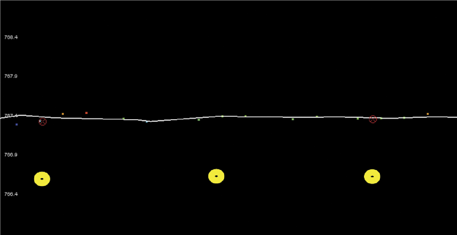
Block-Shifted Data Comparison. In an operational environment, because of systematic errors in the resulting DEM relative to the local height datum, this mean vertical offset is a common occurrence with comparisons against ground control similar to those shown in FIGURE 10. Again, the TIN surface is indicated by the white line, and the ground control points are shown with yellow buffers.
Figure 10. Usual operational comparison of LiDAR surface and ground control points.
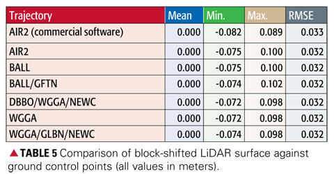
In standard LiDAR operations, the mean vertical offset between the initial results and the ground control, at the control points, produces a zero-mean offset. Following this procedure in this case results in the variation in the comparison of LiDAR data with ground truth now being well within the required limits of 615 centimeters (TABLE 5). The values show that after a block shift, trajectory solutions are virtually identical with a root mean square error of 32 millimeters. Thus, local GNSS reference stations can be replaced by distant CORS sites without loss of accuracy.
Conclusions
A precise wide-area positioning technique for airborne trajectory solutions provides both relative and absolute accuracies similar to those derived from usinga local GNSS reference station. Irrespective of which reference sites are used and once calibration and antenna modeling issues are addressed, the absolute comparison with ground control is well within the required accuracies. With the configuration of a GNSS network such as CORSnet-NSW (when complete, at least one site will always be within 150 kilometers of any point within New South Wales), an airborne LiDAR survey in the network’s service area can provide data for computation of an accurate sensor trajectory. This potentially negates the need to place and maintain ground reference stations close to the survey area — an exercise which not only requires significant resources but also reduces the operational flexibility of the aircraft.
The challenge for this technique in an operational environment is to define and maintain a precise reference frame for all CORSnet-NSW sites and observations, including the use of a stable ellipsoidal height datum with compatible geoid modeling in order to provide local orthometric elevation data. The knowledge base required for computation of wide-area GNSS solutions is significant and requires understanding of geodesy, GNSS positioning, absolute antenna modeling, application of precise ephemerides, and derivation of the other parameters inherent to successful ambiguity resolution over long distances.
Regardless of processing method, a LiDAR survey will always require independent ground surveys for collection of vertical checkpoints, which provide quality control to ensure the accuracy meets specifications, and the means to define any transformations necessary to fit LiDAR data with local height datum.
Manufacturer
NovAtel’s WayPoint GrafNav software was used for comparison purposes.
The ”IT” Software
Runs under Windows, Unix, Linux, and FreeBSD.
Source code compatible with most Fortran compilers.
Follows the IERS 2003 conventions.
Available mainly for collaborative research purposes, with a Free Software Foundation General Public Lice
nse.
Stop-and-go for rapid mobile surveys with pre-surveyed waypoints.
Differential, precise point positioning, mixed mode (precise differential + point positioning).
Data corrected for: Earth tide, neutral atmosphere radio signal delays, carrier phase windup, and so on.
Estimated parameters:
Receiver position in the IGS05 reference frame, with the WGS84 reference ellipsoid, earth spin-rate, light speed, GM constant.
Biases in ionosphere-free carrier-phase linear combination (“floated” ambiguities).
Neutral zenith delay correction error.
Broadcast orbit errors (allows precise differential near-real time solutions).
Integer ambiguity resolution available in differential mode, with short baselines up to 20 kilometers (in minutes), and baselines of unlimited length (in tens of minutes — or just minutes, with a precise ionosphere correction).
Oscar L. Colombo received a degree in electrical engineering from the National University of la Plata, Argentina, and a Ph.D. in electrical engineering from the University of New South Wales, Australia. He is an independent consultant.
Shane Brunker is an airborne LiDAR and imaging specialist working in a consulting capacity for specialized LiDAR survey company Network Mapping (United Kingdom).
Glenn Jones is a senior surveyor at the NSW Land and Property Management Authority in Bathurst, Australia.
Volker Janssen is a GNSS surveyor (CORS Network) in the Survey Infrastructure and Geodesy branch at the NSW Land and Property Management Authority in Bathurst, Australia. He holds a Ph.D. from the University of New South Wales.
Chris Rizos is head of the School of Surveying and Spatial Information Systems of the University of New South Wales, has a surveyor’s degree and a Ph.D. from the same university, and is an specialist in geodesy and GNSS positioning.