Tag: NAPGD2022

Plate tectonics and NGS’s new NSRS terrestrial reference frames
The adoption of the new, modernized National Spatial Reference System (NSRS) is rapidly approaching, with official implementation now expected in the first quarter of 2027.

One of the most common questions I receive during presentations is: How will the National Geodetic Survey (NGS) account for plate tectonics in the modernized NSRS, and what does that mean for my geospatial products and services?

First, I have some very sad news to share.

Dr. Chris Pearson

Our friend and colleague, Dr. Chris Pearson, unexpectedly passed away while in Cape Town attending the May 2026 International Federation of Surveyors (FIG) conference. At the time, he was serving as a Geodetic Advisor for Trimble and as co-chair of FIG Commission 5.2.

Chris previously worked for the National Geodetic Survey (NGS) as a Geodetic Advisor, where he played a key role in developing the comprehensive block model of crustal deformation — widely known as HTDP — across the western United States, including Alaska.

He was an active and respected member of several professional organizations and will be greatly missed by the entire geodetic and surveying community.

Now, let’s discuss how the National Geodetic Survey (NGS) will handle plate tectonics in the modernized National Spatial Reference System (NSRS) and what this will mean for users’ geospatial products and services.

Map of tectonic plates (Image: Dave Zilkoski)

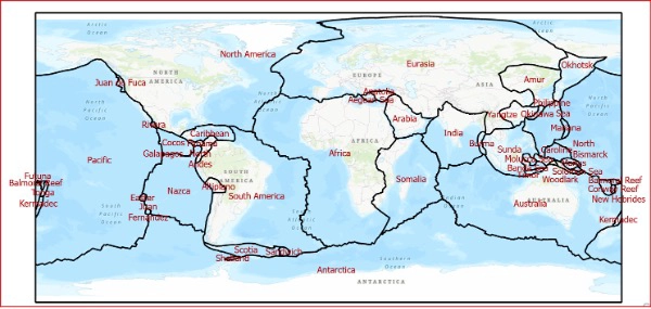
Plate tectonics is the scientific theory that describes how Earth’s outer shell, known as the lithosphere, is divided into large, rigid pieces called tectonic plates. These plates float atop the hotter, more ductile rock in the mantle below and move very slowly — roughly at the same rate as your fingernails grow, about 1 to 10 centimeters per year.

So why does plate tectonics matter for geodetic coordinates? Because the most significant geological activity — including earthquakes, volcanic eruptions, and crustal deformation — occurs primarily at the boundaries where these plates interact.

My last newsletter highlighted several activities by the North Carolina 2022 Reference Frame Working Group (NC RFWG) that are addressing this issue and other challenges related to the implementation of the new NSRS.

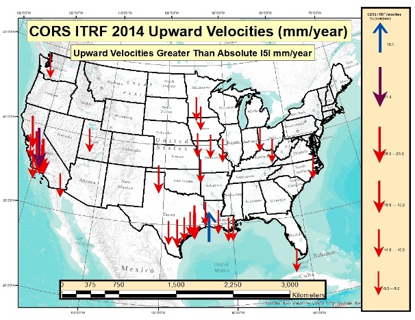
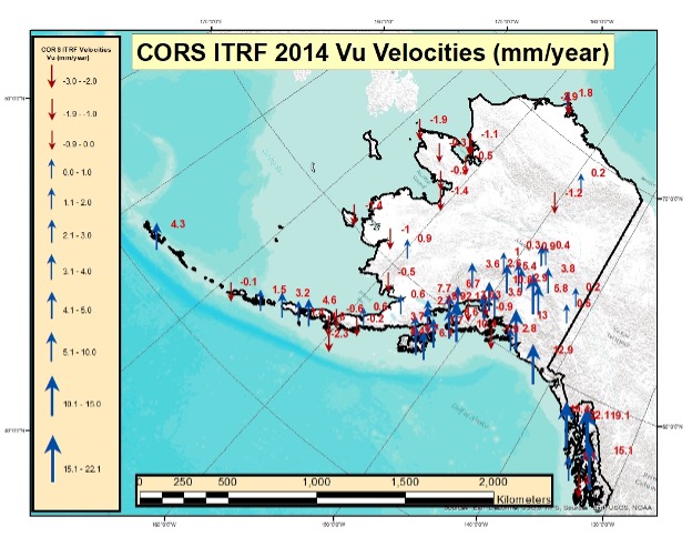
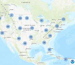
During my presentations on the modernized NSRS, I always show the National Geodetic Survey (NGS) maps that illustrate the approximate horizontal and vertical changes expected when the new Terrestrial Reference Frames (TRFs) are adopted, with coordinates referenced to epoch 2020.00. These maps provide a high-level (“30,000-foot”) overview of the anticipated changes. However, they do not include the level of detail that many users are looking for.

Participants at these seminars and meetings consistently want to know the expected coordinate differences for their specific state or local region, and how the time-dependent components will impact their work.

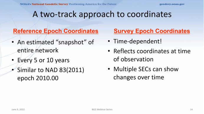
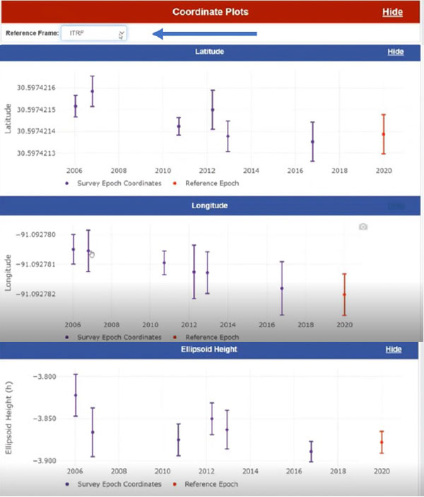
Most geospatial users now understand that International Terrestrial Reference Frame (ITRF) coordinates include a velocity component caused by tectonic plate movement. To manage these changing coordinates, the National Geodetic Survey (NGS) plans to incorporate time-dependent modeling. NGS has developed two key models — EPP2022 and IFDM2022 — to make time-dependent geodetic control practical and usable.
- EPP2022 (Euler Pole Parameters) describes the rigid rotation of tectonic plates.
- IFDM2022 (Intra-Frame Deformation Model) computes the internal deformation and drift within a tectonic plate.
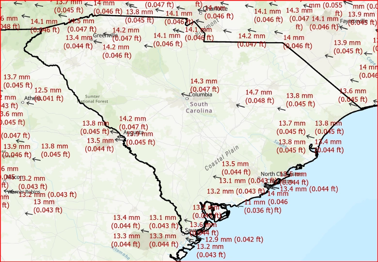
As shown in the figure below, the NOAA CORS Network station COLA in Columbia, South Carolina — located on the North American Plate — is moving at approximately 0.05 feet (14 mm) per year.

This velocity is provided on the published ITRF2020 position and velocity data for the station (NGS CORS Position and Velocity Sheet for COLA). As a result, a surveyor working in June 2026 would observe a shift of about 0.3 feet in the ITRF2020 horizontal coordinates compared to the 2020.00 reference epoch, solely due to tectonic plate motion.

Motion due to plate movement (rates per year) – based on ITRF2020 velocity rates

(Image: Dave Zilkoski)

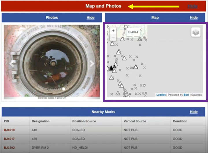
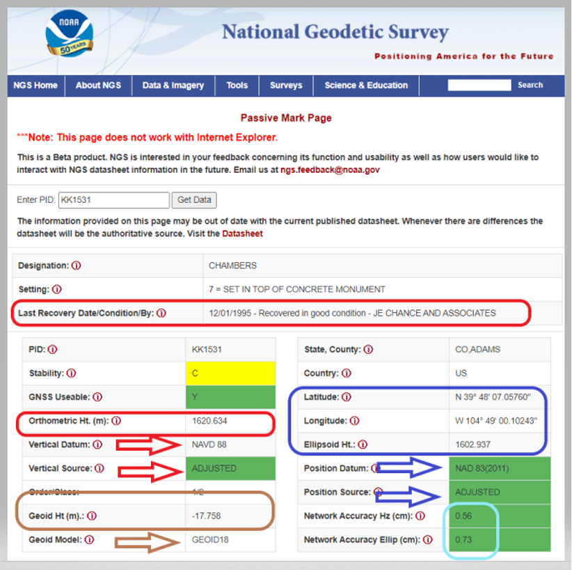
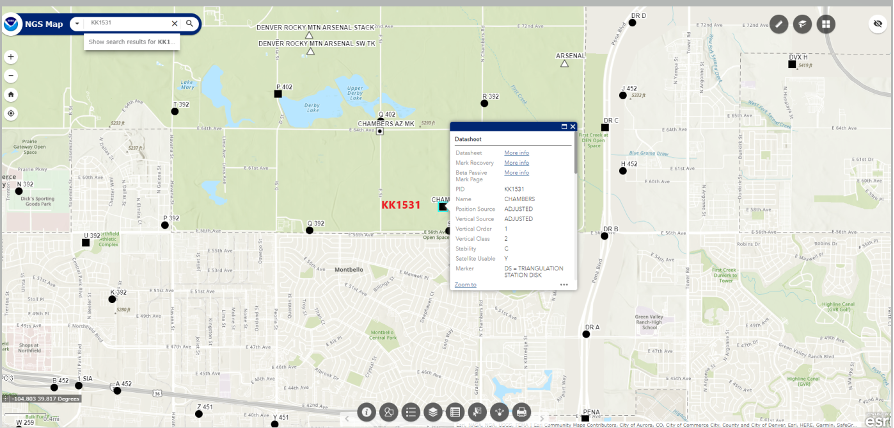
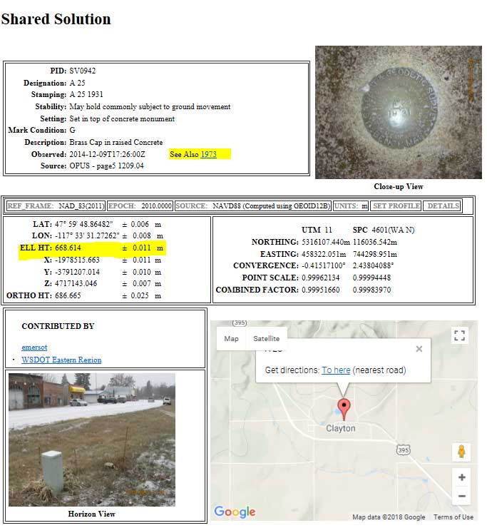
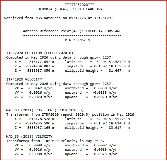
The National Geodetic Survey (NGS) provides detailed information for all NOAA CORS Network (NCN) stations on the NGS NCN Station Pages.

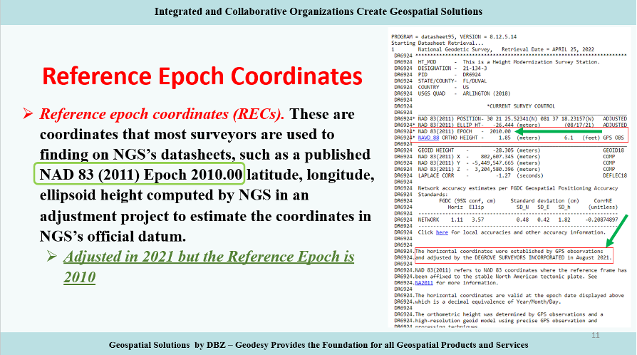
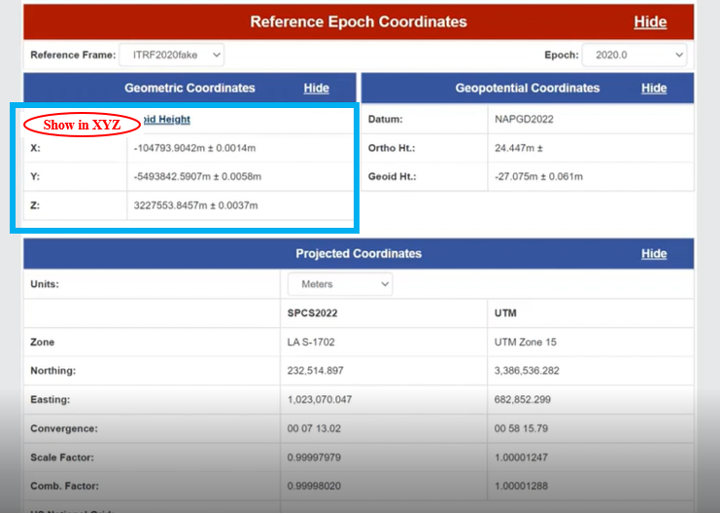
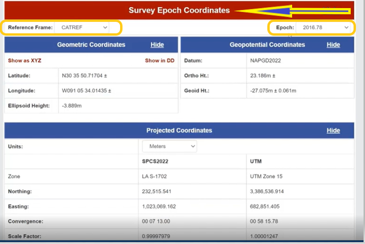
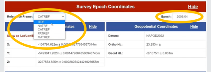
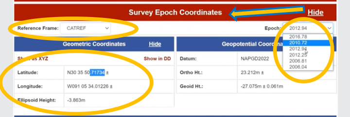
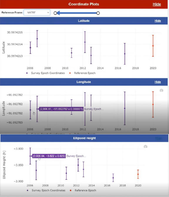
In the section titled “Coordinates and Velocities”, simply click the Position and Velocity button to view the station’s ITRF2020 coordinates and velocities (referenced to epoch 2020.00), as well as the NAD 83 (2011) coordinates and velocities (referenced to epoch 2010.00).

NGS CORS position and velocity sheet for COLA

So, what does this mean for users?

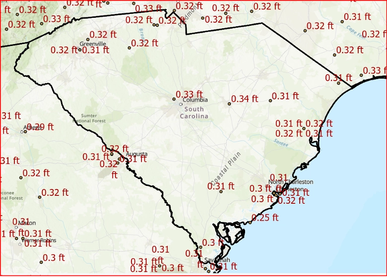
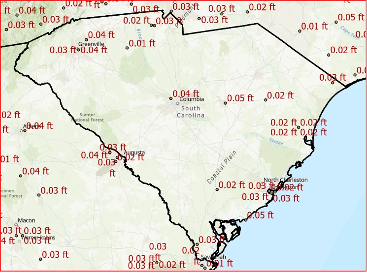
As previously mentioned, the National Geodetic Survey (NGS) is expected to adopt the new modernized NSRS in the first quarter of 2027. The figure below shows the change in ITRF2020 coordinate values between epoch 2020.00 and 2027.00 for NOAA CORS Network (NCN) stations in South Carolina. This shift of approximately 0.33 feet (10 cm) is the result of seven years of tectonic plate motion.

ITRF2020, Epoch 2020 to ITRF2020, Epoch 2027 (units ift)

Image: Dave Zilkoski

That said, what will the change in NATRF2022 coordinate values be between epoch 2020.00 and 2027.00?

This is where NGS’s EPP2022 and IFDM2022 models become essential. My February 2022 and July 2024 GPS World newsletters discussed the Euler Pole Parameters (EPP) process in detail.

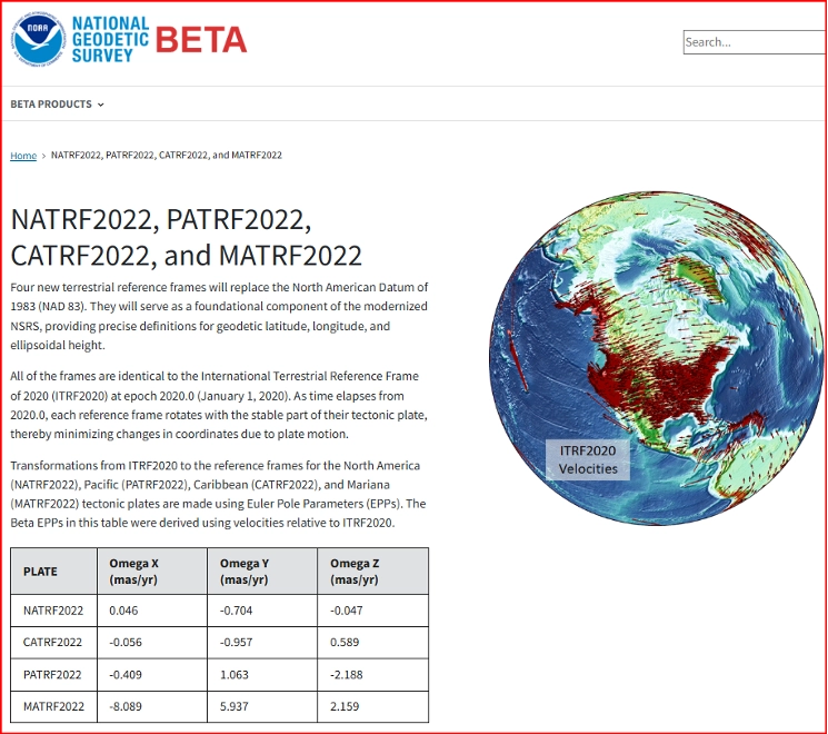
The Beta NATRF2022 website provides the Euler Pole Parameters (EPP) needed to define the relationship between ITRF2020 and the new NATRF2022 frames for the North American, Caribbean, Pacific, and Mariana plates, as outlined in NGS’s Blueprint Part 1 document. The values in the table have proven especially useful to programmers developing and testing their software.

Beta Values for EPP

(Image: NGS)

As stated in Blueprint Part 1, the National Geodetic Survey (NGS) will define the official relationship between ITRF2020 and the four NSRS Terrestrial Reference Frames (TRFs) through Equation 59. This equation uses the rotation matrix provided in Equation 58, which results in Equation 60.

See the box titled “Official Relationship Between ITRF2020 and the Four NSRS TRFs” for the equations.

Official relationship between ITRF2020 and the four NSRS TRFs

(Image: NGS Blueprint pt. 1)

So, what does this mean for surveyors?

The primary purpose of the EPP2022 model is to remove the rigid tectonic plate motion from the coordinates. After applying the EPP2022 model to the ITRF2020 coordinates at epoch 2027.00, the resulting NATRF2022 horizontal coordinates for station COLA (epoch 2027.00) will change by only 0.04 feet (12 mm).

EPP applied

NATRF2022, Epoch 2020 to NATRF2022, Epoch 2027 in SC (units ift)

Image: Dave Zilkoski

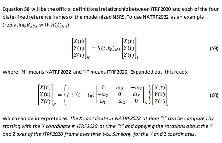
As shown in the figure, the EPP2022 model removes most of the horizontal movement caused by seven years of tectonic plate motion — reducing it to just 0.04 feet (1.2 cm) at station COLA. In other words, the EPP model effectively removes the vast majority of plate tectonic effects.

Additionally, the plot shows that the relative horizontal differences between nearby marks are very small — typically less than 0.01 feet (0.3 cm).

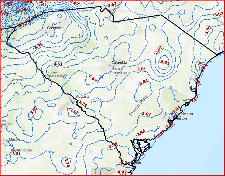
As previously mentioned, the NGS maps provide a high-level (“30,000-foot”) view of the expected changes between the current NSRS and the new modernized NSRS. So, what are the anticipated differences between NAD 83 (2011) and NATRF2022 specifically in South Carolina?

The figures below illustrate the differences in both horizontal position and ellipsoid heights between NAD 83 (2011) and NATRF2022 coordinates across South Carolina.

NAD83 (2011), Epoch 2010 to NATRF2022, Epoch 2020 Horizontal Changes in SC (Units ift)

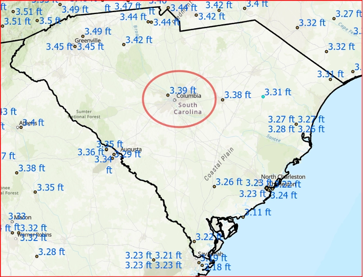
NAD83 (2011), Epoch 2010 to NATRF2022, Epoch 2020 Ellipsoid Height Changes in SC (Units ift)

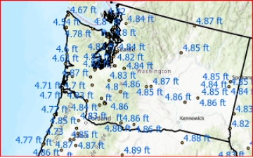
The magnitude of these changes varies depending on your location. To illustrate this, I’ve provided two additional examples: one for Iowa and one for Washington State. As the plots clearly show, the differences in these states are noticeably different from those depicted for South Carolina.

NAD83 (2011), Epoch 2010 to NATRF2022, Epoch 2020 Horizontal Changes (Units ift)

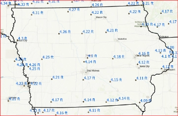
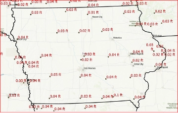
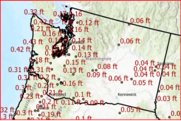
That said, the differences between NATRF2022 at epoch 2020.00 and epoch 2027.00 in Iowa and Washington State — after applying the EPP2022 model — are very similar to the values shown for South Carolina.

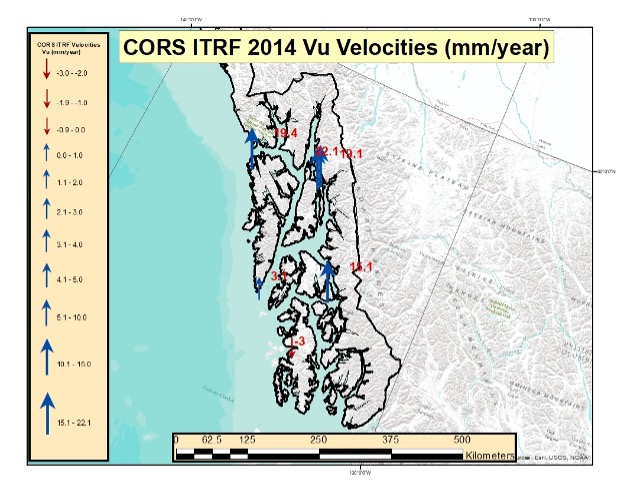
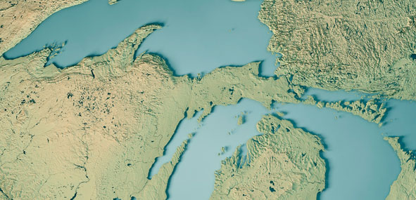
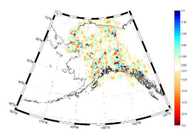
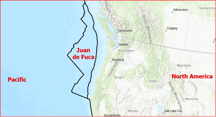
However, readers should note that the differences in Washington State increase as you move toward the coast. This is because the area lies near the boundary between the North American Plate and the Pacific Plate. The Juan de Fuca Plate, a small microplate in the eastern North Pacific, is also actively involved in this region.

(See the box titled “Juan de Fuca Plate.”)

NATRF2022, Epoch 2020 to NATRF2022, Epoch 2027 (units ift)EPP Applied

Juan de Fuca Plate

The Juan de Fuca plate or Juan de Fuca microplate is a small oceanic tectonic plate (microplate) generated from the Juan de Fuca Ridge that is subducting beneath the northerly portion of the western side of the North American plate at the Cascadia subduction zone.

Image: Dave Zilkoski

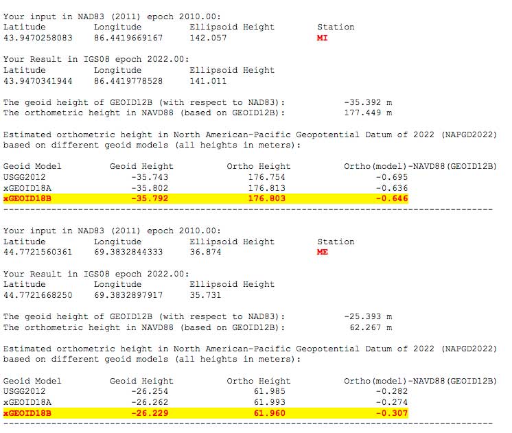
What about orthometric height changes in the new NSRS?

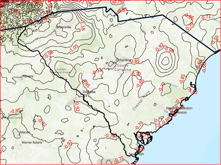
As an example, the orthometric height differences between NAPGD 2022 and NAVD 88 in South Carolina are expected to range from approximately -0.8 feet to -1.3 feet.

Difference between NAPGD2022 and NAVD 88 (Units ift) in S.C.

Image: Dave Zilkoski

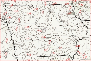
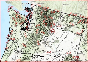
The differences between NAPGD 2022 and NAVD 88 vary significantly depending on your location. The figures below illustrate these orthometric height differences for Iowa and Washington State as examples.

Difference between NAPGD2022 and NAVD 88 (Units ift)

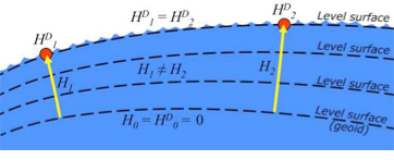
The new NSRS will use a gravimetric geoid (GEOID2022) rather than a hybrid geoid (GEOID18) to compute GNSS-derived orthometric heights.

During my presentations, I always remind participants that a hybrid geoid is not a “true” geoid. It is simply a transformation model that converts ellipsoid heights in one reference frame to orthometric heights in a specific vertical datum. Specifically, GEOID18 is a transformation tool that allows users to derive NAVD 88 orthometric heights from NAD 83 (2011), epoch 2010 ellipsoid heights.

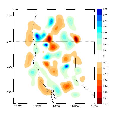
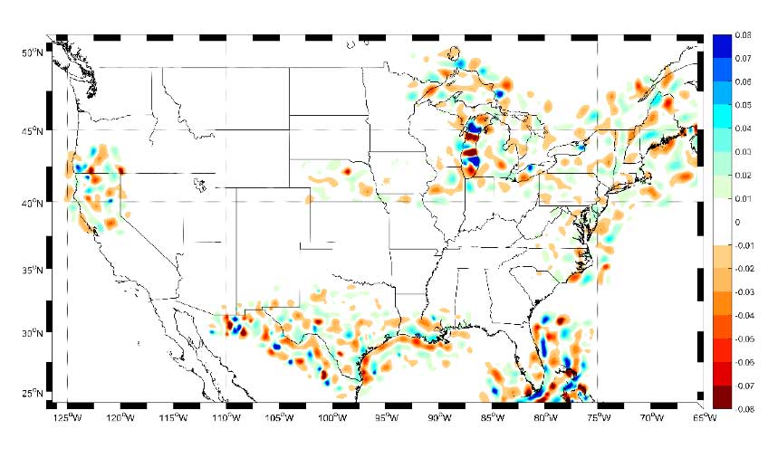
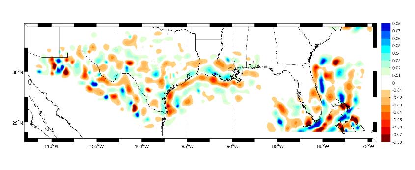
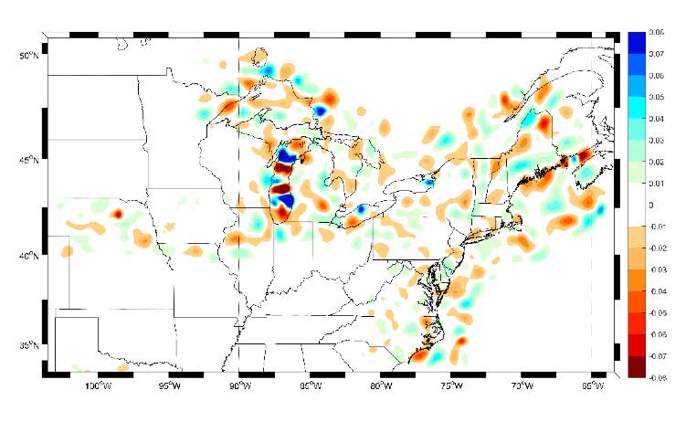
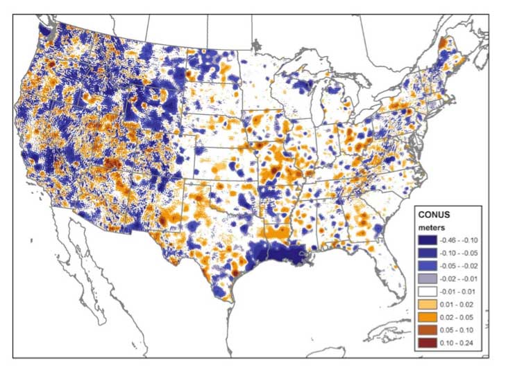
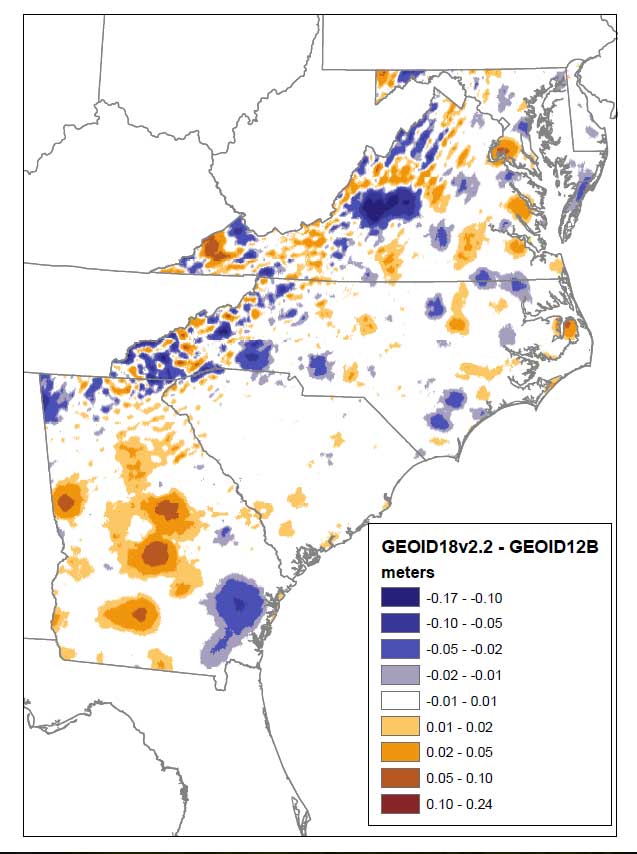
The figure below shows the differences between the gravimetric geoid model GEOID2022 and the hybrid geoid model GEOID18.

Important note: Users cannot use GEOID18 with NATRF2022 ellipsoid heights to obtain NAVD 88 orthometric heights. Instead, GEOID2022 must be used with NATRF2022 ellipsoid heights to compute orthometric heights in the new vertical datum, NAPGD 2022.

Differences between GEOID2022 and GEOID18 in SC (Units ift)

As noted at the outset of this newsletter, the transition to the modernized National Spatial Reference System (NSRS) is rapidly approaching, with official implementation scheduled for the first quarter of 2027.

The National Geodetic Survey (NGS) released the following announcement on May 28, 2026:

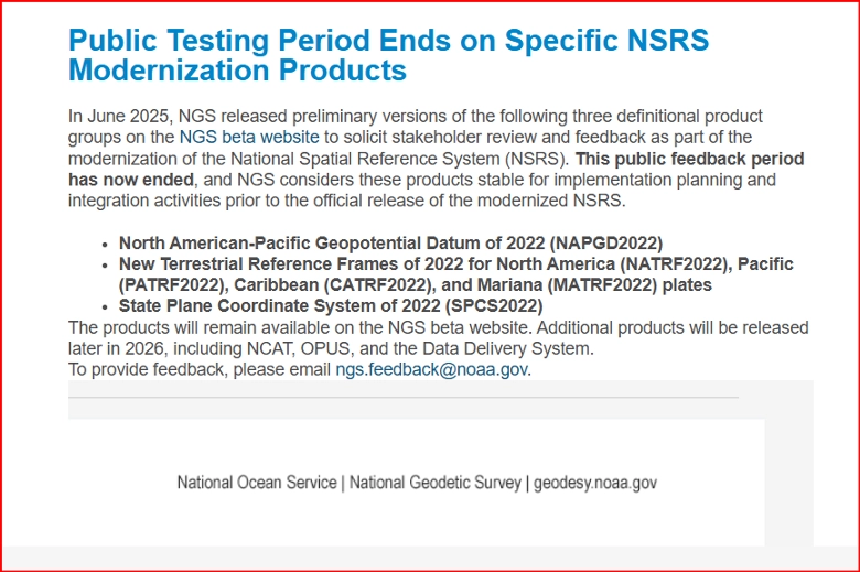
Public Testing Period Ends for Key NSRS Modernization Products

NGS has declared the following products stable and ready for implementation planning and integration activities ahead of the official release:
- North American-Pacific Geopotential Datum of 2022 (NAPGD2022)
- New Terrestrial Reference Frames of 2022:
  - North America (NATRF2022)
  - Pacific (PATRF2022)
  - Caribbean (CATRF2022)
  - Mariana (MATRF2022)
- State Plane Coordinate System of 2022 (SPCS2022)
Additional modernization products, including NCAT, OPUS, and the Data Delivery System, are scheduled for release later in 2026.

NGS news

Public testing period ends on specific NSRS modernization products

Image: NOAA

Image: NOAA

This newsletter highlighted the role of the EPP2022 model in accounting for plate tectonics and illustrated the anticipated local differences between the current National Spatial Reference System (NSRS) and the upcoming modernized version.

Future editions will continue to explore additional NGS Beta products as they are released later in 2026.
June 3, 2026
What will the data delivery system of the modernized 2022 NSRS look like?
My previous column highlighted that orthometric heights in NAPGD2022 will be defined through ellipsoid heights and a geoid model, such as GEOID2022. Therefore, changes in the geoid model will be very important to users estimating orthometric heights using GNSS. I briefly described the geophysical reasons for changes in the geoid that affect the orthometric height of a mark.

For the past four years, I have discussed in my columns the tasks associated with the new, modernized 2022 reference frames. It’s now the middle of 2022, so where are the new reference frames? Well, on June 9, Dru Smith, NSRS modernization manager for the National Geodetic Survey (NGS), provided an update on the status of the modernization in a webinar. The Powerpoint slides and video of the presentation can be downloaded from the NGS website under the following title: It’s 2022…Are You Done Yet? I will highlight some of the items from the webinar, but I encourage everyone to download the video and listen to the webinar.

First, Smith mentioned that NGS will be providing new types of coordinates. The NGS denotes this as a two-track approach to coordinates: Reference Epoch Coordinates (REC) and Survey Epoch Coordinates (SEC). See the box below.

New types of coordinates (Image: NGS June 6 webinar)

Reference Epochs Coordinates (REC) are defined in NGS Blueprint for the Modernized NSRS, Part 3 as coordinates computed by NGS in an adjustment project to estimate the coordinates at one of the official reference epochs that NGS will define in 2025. RECs are similar to coordinates computed by NGS in a nationwide adjustment project such as the National Adjustment of 2011 (see the box below).

NAD 83 (2011) epoch 2010.00 coordinates (Image: NGS)

NGS has not determined what data will be included in the first iteration of RECs. For the 2020.00 project, the current cutoff date for incorporating data is Dec. 31. Users can submit the data to NGS via OPUS projects and the OPUS-Share tool. To increase the submission of GNSS observations on marks, NGS has developed a beta OPUS-Projects 5.0 webtool that will allow real-time kinematic and real time network (RTK/RTN) observations to be submitted.

As previously mentioned, at this time, the NGS has not determined the cutoff for the earliest data to be included in the determination of the 2020.00 RECs. The agency will be conducting experiments to determine the appropriate cutoff date. These coordinates will require an intra-frame velocity model (IFVM) to generate the RECs at the specific reference epoch.

As of February 2021, based on NGS’ Blueprint for the Modernized NSRS, Part 3, version February 2021, the following is the agency’s policy with regard to RECs:
- For a given mark and a given reference epoch, the REC will never be changed–except to correct a blunder.
- This does not prevent NGS from adding new RECs
  - on points with new data that have not yet had an REC computed
  - for marks that do not have an REC in the most recently passed reference epoch, a new REC can be computed and added to the NSRS.
- Per NGS’ Blueprint for the Modernized NSRS, Part 3, version February 2021, for simplicity, RECs may happen on the same schedule as SECs.
Survey epoch coordinates (SECs) are defined as coordinates computed by NGS at a specific survey epoch. Users will submit their data and its metadata to NGS, and NGS will then check, adjust and define the coordinates at one “survey epoch.” These coordinates will be “part of the NSRS,” Smith said. NGS is computing coordinates in this manner to provide the best estimate of the coordinates at any mark at a specific moment in time, which is very important in areas influenced by crustal movement.

So, how will NGS process and generate these SECs?

Survey epoch coordinates (SECs) are designed to provide time-dependent geodetic coordinates. Therefore, NGS has to choose some time span in which all observations will be processed together to yield a single SEC of a mark. NGS denotes this time span as a “geometric adjustment window.” NGS wants the adjustment window to be short enough so that movement of a mark did not occur between repeat observations (or was small enough to be ignored) and long enough for users to efficiently and effectively collect redundant observations for submission to NGS (see the box below).

Proposed SEC geometric adjustment window. (Image: NGS)

As of February 2021, based on the NGS Blueprint for the Modernized NSRS, Part 3, the following is the policy with regard to SECs:
- One or more GNSS occupation(s) over a single mark will be processed into one survey epoch coordinate when all occupations take place within one geometric adjustment window.
- If a user submits two occupations on one mark, but they happen to fall in two consecutive geometric adjustment windows, NGS will use them to create two distinct survey epoch coordinates. Each SEC will be based on one occupation.
Future columns will provide more explanation about this concept of a geometric adjustment window and how NGS will process the data to generate survey epoch coordinates.

NGS is developing models and tools for users to submit data to NGS to compute coordinates — including OPUS coordinates, reference epoch coordinates and survey epoch coordinates. Figure 9 from Blueprint for the Modernized NSRS, Part 3, version February 2021, is a schematic that shows the flexibility NGS is building into an OPUS-type webtool. Basically, if users follow NGS guidelines and rules, and submit their data to NGS, then NGS will compute and publish REC and SEC coordinates (see the blue outline in the box below). If users only want to compute OPUS coordinates, then they can use NGS’s webtool without submitting the data to NGS (see the red outline in the box below).

Building flexibility into OPUS (Image: NGS)

Dru Smith’s June 9 update on the status of the modernization provided a mockup of how users will be able to retrieve data using their web browsers — a prototype is being developed. The data will also be available in downloadable form such as an XML file for users to input the data and metadata into their programs or databases. I recently discussed some of this material at seminars I presented at the Florida Surveyors and Mapping Society’s 67th annual conference held in Palm Beach Gardens. The participants were very interested in the prototype, but really wanted to learn more about the format and process of the downloadable XML files. I’m sure future NGS webinars will address this topic. I emphasized to the group that they should watch the entire presentation and provide feedback to NGS. As mentioned above, Powerpoint slides and video can be downloaded from the NGS webinar website.

The boxes below highlight a few of the options NGS is considering. The box “Data Delivery – Prototype” is an example provided by Smith during his webinar. It should be noted that the images of the prototype are not included in the downable slides, but they are part of the video. The images presented in this column are screen captures from the video.

Data delivery prototype. (Image: NGS)

The box below provides some of the basic information of a mark, such as its PID, name, stability, GNSS usable code, setting and the latest recovery information. Again, this is a prototype, so users should feel free to send feedback to NGS. NGS wants to generate a usable product, and is interested in user feedback.

Primary information prototype. (Image: NGS)

As previously stated, NGS is implementing a two-track approach to coordinates: publishing REC and SEC. The box below provides the REC information of a mark when a user clicks the “Show” button. As shown in the diagram, the reference frame and epoch are provided, as well as the geometric coordinates (latitude, longitude, ellipsoid height) and geopotential coordinate information (NAPGD2022 orthometric height and geoid height).

Reference epoch coordinates prototype. (Image: NGS)

NGS provides an option for individuals who want the geometric coordinates in the X, Y, Z format (see the box below). Remember, this is only a mockup of a prototype, to give us an idea of the direction NGS is going with its data delivery system in the new, modernized 2022 NSRS.

REC Shown in X,Y,Z. (Image: NGS)

Similar to the REC, the prototype includes SEC. For a mark, the latter are different from the former because SEC are computed at the epoch of the survey observations (see the box below).

Survey epoch coordinates – prototype. (Image: NGS)

The box titled “SEC in CATRF – Prototype” is an example of a mark in the CATRF reference frame and the survey epoch of 2012.94. As indicated in the diagrams, users will be able to select the reference frame (ITRF, NATRF, CATRF, PATRF and MATRF) and the survey epoch.

SEC in CATRF – Prototype

Option to Select Survey Epoch

Options to select reference frame (Images: NGS)

Another feature of the data delivery system is that it provides plots of a mark’s survey epoch coordinate values at different epochs. In the example shown in the box below, the plots provide values of a mark’s latitude, longitude and ellipsoid heights based on each survey epoch data. The user can select various reference frames of the mark to understand the change based on the reference frame.

Coordinate plots in ITRF prototype. (Image: NGS)

The box below clearly shows a slope in the changes in coordinates based on survey epochs, especially in the longitude. This is the plate rotating in time. You can see the changes in latitude, longitude and ellipsoid height in the NATRF reference frame for the same mark. The latitude and longitude plots do not show a slope because the plate rotation is removed using a model to change from the ITRF reference frame to the NATRF reference frame. That said, the ellipsoid height plots look the same because the rotation model does not change the ellipsoid height.

Coordinate plots in NATRF prototype. (Image: NGS)

The prototype also provides maps, photos and descriptive text of the mark.

Map and photos of a mark in the prototype. (Image: NGS)

Descriptive text prototype (Image: NGS)

Some of this data delivery output may seem familiar to users who have used the NGS beta routines (see the box below).

Beta Routines

Beta routines (Image: NGS)

For example, the Passive Mark Page Webtool provides the coordinate information for a mark. My October 2020 column described the tool is detail. See below for an example of the passive mark tool.

Beta Passive Mark of KK1531 (Image: NGS)

The NGS Beta Map routine enables users to link to NGS datasheets, the passive mark tool and mark recovery, as well as connect to OPUS Shared Solutions and the NOAA CORS Network. See below for an example. It also provides a measuring tool, multiple basemaps and the ability to export data. My December 2021 column described the NGS Beta Map in detail.

Example of NGS Beta Map Routine for KK1531 (Image: National Geodetic Survey)

Only three years remain before the release of the new, modernized NSRS. I encourage everyone to try all of the beta products, and download Dru Smith’s June 6 webinar for a better understanding of the agency’s current thoughts on how it will provide data to users in the new, modernized NSRS. As for all the NGS beta products, the agency would like users to try the tools and provide feedback on what they liked and what they didn’t like, as well as any additional information you need or would like to see. The NGS is trying to develop tools useful to everyone, but that won’t be possible unless they hear from users.

The following statement on NGS beta products explains how to provide feedback and why it is important:

“This is a beta product. NGS is interested in your feedback concerning its function and usability as well as how users would like to interact with NGS datasheet information in the future. Email us at [email protected].”
August 3, 2022
The effects of vertical movement on NGS’s modernized 2022 NSRS
My February column explained why it is important to account for horizontal movement of marks everywhere, and not just in areas influenced by active crustal movement due to earthquakes such as Southern California.

It provided information about the NOAA CORS Network (NCN) rates of movement based on International Reference Frame of 2014 (ITRF2014) coordinates and horizontal velocity information. It highlighted reports from the National Geodetic Survey (NGS) that describe models that will facilitate users transferring coordinates between reference frames and dealing with intra-frame movement between marks based on surveys performed at different epochs.

NAPGD2022 orthometric heights will primarily be accessed through GNSS technology.

As I stated in my February column, this is not just a horizontal positioning issue. In this month’s column, I address estimates of vertical movement that will have to be accounted for in the new, modernized National Spatial Reference System (NSRS).

The NGS 2021 revised Blueprint 2, NOAA Technical Report NOS NGS 64 Blueprint for the Modernized NSRS, Part 2: Geopotential Coordinates and Geopotential Datum, addresses the geopotential aspects of the new, modernized NSRS. The modernized Geopotential Datum will be called the North American-Pacific Geopotential Datum of 2022 (NAPGD2022). There will be four primary, interrelated time-dependent products of NAPGD2022:
- a global model of Earth’s geopotential field (GM2022)
- regional gridded geoid undulation models (GEOID2022)
- regional gridded deflection of the vertical models (DEFLEC2022)
- regional gridded surface gravity models (GRAV2022).
NAPGD2022 will provide gridded models for North America (that includes CONUS, Alaska, Hawaii, the Caribbean, Canada, Mexico, Central America and Greenland), American Samoa and Guam/Commonwealth of Northern Mariana Islands (CNMI). My previous columns have described the NAPGD2022 in detail. The revised NOS NGS 64 report mentioned that NAPGD2022 will be built upon ITRF2020. It states that NAPGD2022 will operate equally well in any of the four new terrestrial reference frames developed as part of the new, modernized NSRS in 2022.

As I stated in previous columns, orthometric heights in NAPGD2022 will be defined through GNSS ellipsoid heights and GEOID2022. This means NAPGD2022 orthometric heights will primarily be accessed through GNSS technology. GEOID2022 will be defined in a manner that best fits global mean sea level at the epoch of NAPGD2022.

As in my previous column, to better visualize the potential size of the vertical movement, I used the CORS ITRF2014 coordinates and velocities from the NGS website to create plots depicting the upward velocity (Vu) values for CORS that are designated as operational and have computed velocities. [Note: I use the term upward because that is how it is reported on the NGS CORS website under the tab labeled “position and velocity.” The term upward velocity means movement in both directions — negative is downward and positive is upward.] The box below shows maximum, minimum, average and standard deviations of upward velocity values for each state and territory of the United States.

Table of ITRF 2014 Upward Velocities of US CORSs

The upward velocity values are not as systematic as the horizontal velocity values, and they are significantly smaller. I have highlighted the average value velocity column. As indicated in the table, the values vary from state to state, but they are all small relative to the horizontal movement values. (See my previous column for plots depicting the horizontal values.)

What is interesting is the range of values in some states. For example, Alaska and California have a very large range — understandable because of the active earthquakes and other movement that occur in these states. Also, Louisiana and Texas have a very large range due to local subsidence.

I decided to highlight the values for the conterminous United States (CONUS) in two separate plots. The box “Upward Velocities (Vu) Between +/–5 mm/year in CONUS” depicts upward velocities (Vu) between +/–5 mm/year in CONUS. The box “Upward Velocities Greater than Absolute Values of 5 mm/year in CONUS” depicts upward velocity values greater than +/–5 mm/year.

Upward Velocities (Vu) between +/- 5 mm/year in CONUS

Image: Dave Zilkoski

It’s obvious that most of the vertical movement values are between +/–5 mm/year in CONUS. There are some large values in California, Louisiana and Texas. This is highlighted in both plots.

Upward Velocities (Vu) Greater than Absolute Values of 5 mm/year in CONUS

(Image: Dave Zilkoski)

As indicated in the plots, some of the values exceed 10 mm/year. In five years, the heights of marks in these regions could potentially change by 5 cm. An example of the potential subsidence in the Houston-Galveston, Texas, region is depicted in the box below. As indicated in the plot, some marks are subsiding greater than 2 cm/year. That means in five years the marks in that region could have subsided more than 10 centimeters.

Estimate of Subsidence in the Houston-Galveston, Texas, Region

Harris-Galveston Subsidence District Website

The box below depicts the values in Alaska. Most of these values indicate that the marks are uplifting. Some of these values exceed 10 mm/year. Once again, height coordinates in some regions will potentially change 5 cm in five years. I generated a separate plot for the southeastern region of Alaska. (See the box titled “Upward Velocities (Vu) in Southeastern Alaska.”)

Upward Velocities (Vu) in Alaska [All Values]

Image: Dave Zilkoski

Upward Velocities (Vu) in Southeastern Alaska [All Values]

Image: Dave Zilkoski

As I did in my previous columns, I prepared several plots that depict the upward velocities in various regions of the United States. See the boxes below for North Carolina, Missouri Southwest U.S. The plots indicate that the magnitude of the vertical movement varies from state to state, as well as within the states.

CORS ITRF 2014 Upward Velocities (Vu) in Missouri [All Values]

Image: Dave Zilkoski

CORS ITRF 2014 Upward Velocities (Vu) in Southwest U.S. [All Values]

Image: Dave Zilkoski

CORS ITRF 2014 Upward Velocities (Vu) in Southwest U.S. [Values Between +/- 5 mm/year]

Image: Dave Zilkoski

I also generated plots that separately depict the positive and negative upward velocities for the conterminous United States. There are more negative upward velocity values than positive values.

CORS ITRF 14 Positive Upward Velocities (Vu) in Conterminous U.S. (Values between 0 and 5 mm/year)

Image: Dave Zilkoski

CORS ITRF 2014 Negative Upward Velocities (Vu) in Conterminous U.S. (Values between -5 and 0 mm/year)

Image: Dave Zilkoski

The table below provides the number of CORS with negative upward velocity values and the number of CORS with positive values for every state and territory of the United States. I have highlighted the states and territories that have more positive values than negative values. As you can see, only six states have more positive upward velocities than negative values. Four of the six states are in Northeastern United States.

Table of ITRF 2014 Positive and Negative Upward Velocities for United States

So far, this column has only addressed the vertical movement at the NCN CORS. The values at the sites indicate the potential movement of marks in the area of the CORS. The rates are based on GNSS data and have an estimate of error associated with them.

I’m not sure how NGS will address the vertical movement effects in the new, modernized NSRS. That said, NGS will be monitoring the CORS and looking for trends to help describe the movement at the CORS. These trends will be an indication of what may be happening in the area.

In addition to the movement of individual marks, there are geophysical reasons for changes in the geoid. As I stated in previous columns, orthometric heights in NAPGD2022 will be defined through ellipsoid heights and GEOID2022. Therefore, changes in the geoid model will be very important to users estimating orthometric heights using GNSS.

As stated in the NGS 64 report, NGS has set a goal of maintaining geoid accuracy at 1 centimeter (1 standard deviation) in both absolute and differential geoid undulations. Figure 13 from the NGS 62 Report depicts an estimate of the secular change in the geoid. As indicated in the plot, the changes are very small, ranging from –1.25 mm/year to 1.5 mm/year.

What I find interesting is the small negative change in the southeastern United States. There are other drivers for geoid changes. Future columns will address some of these changes and what it means to users.

Figure 13 from NOS NGS 62 Report

Image from NGS website: Blueprint 2 Revised NOAA_TR_NOS_NGS_0064.pdf

Figure 13 – Secular Geoid Change

Lastly, I’d like to highlight a new service from NGS: “NGS Webinar Series Certificates of Attendance.” See the box titled “Ways to Earn a Certificate of Attendance.” Basically, users can earn certificates by viewing a webinar after it has been posted by NGS. This is very useful for users who could not attend the original webinar. I encourage all users to check out the site to find out more information about the new service.

Ways to Earn a Certificate of Attendance

Image from NGS website: https://geodesy.noaa.gov/web/science_edu/webinar_series/certificates.shtml
April 6, 2022

FIG workshop delves into Great Lakes, highlights GNSS techniques

Image: FrankRamspott/iStock/Getty Images Plus/Getty Images

In one of my previous columns, I described the National Geodetic Survey’s (NGS) plans for replacing the North American Vertical Datum of 1988 (NAVD 88) with the North American-Pacific Geopotential Datum of 2022 (NAPGD2022).

As stated in the NOAA Technical Report NOS NGS 64 Blueprint for the Modernized NSRS, Part 2: Geopotential Coordinates and Geopotential Datum, November 2017, recently revised in February 2021, orthometric heights in NAPGD2022 will be defined through ellipsoid heights and GEOID2022. This means NAPGD2022 orthometric heights will primarily be accessed through GNSS technology.

Like NAPGD2022, in the next update of the International Great Lakes Datum, denoted as IGLD (2020), the heights in the Great Lakes Region will be developed from GNSS and a gravity model. Unlike NAPGD2022, where users will be estimating GNSS-derived orthometric heights, IGLD (2020) users will be estimating GNSS-derived dynamic heights using GNSS and a gravity model.

As president of the American Association for Geodetic Surveying (AAGS), I participated in the International Federation of Surveyors (FIG) Virtual Working Week 2021 held June 20–25. For those unfamiliar with AAGS, some activities AAGS pursues are below.

AAGS Activities

Promote a better understanding of geodesy as a science;
Create a better appreciation of the value of geodetic surveys and thus encourage greater use of such surveys;
Promote geodetic surveys by individuals, government, and private organizations;
Foster the adoption of uniform standards and procedures for completing geodetic surveys;
Promote the processing, publishing, and disseminating of geodetic survey data and information;
Promote programs for testing, calibrating, and evaluating geodetic equipment;
Further the development and implementation of the Global Navigation Satellite System (GNSS) for geodetic, land surveying, and land information system applications;
Inform the membership of new technical developments by meetings of the association and publications in Surveying and Land Information Science (SaLIS);
Promote educational programs in geodesy, geodetic surveying, and related fields;
Cooperate with other similar organizations, both national and international, in support of the science of geodesy;
Encourage the use of geodetic surveys and mathematical coordinate systems in establishing Public Land Survey System (PLSS) corners

As stated above, AAGS cooperates with other similar organizations, both national and international, in support of the science of geodesy. AAGS is a voting member of FIG, which means AAGS has the opportunity to nominate and vote for elected officials, and develop policy that is important to all surveyors and mappers.

On a side note, AAGS is always looking for new members that want to help promote geodetic surveying and related topics.

The theme of the FIG Working Week 2021 virtual conference was “Smart Surveyors for Land and Water Management: Challenges in a New Reality.” FIG Commission 5 focuses on meeting the highest level of accuracy for positioning and measurement (see box titled FIG Commission 5). Five 90-minute sessions described some of the efforts of FIG Commission 5.

FIG Commission 5

“FIG Commission 5 focuses on meeting the highest level of accuracy for positioning and measurement. It provides the tools, techniques and procedures to educate and train surveying professionals everywhere. Appropriate methodology for data collection and processing are required to be successful in an era of global, integrated geospatial data.”

These sessions raised surveyor awareness of cutting-edge technology, techniques and procedures for using geodetic data and enhanced global cooperation and standardization in conformance with the ideals expressed by the United Nations resolution for a Global Geodetic Reference Frame. There were many good papers on positioning and measurement presented at the virtual meeting. Readers can obtain a list of presentations and papers at this website.

A paper by Jacob Heck, U.S National Geodetic Survey, and Michael Craymer, Canada Geodetic Survey titled “Updating the International Great Lakes Datum: Enabling the Integration of Water and Land Management in the Great Lakes Region” should be of interest to many U.S. and Canadian surveyors. The box below provides a link to the abstract, paper, handouts and video of the presentation.

Commission 4 and 5 Joint Session

Tuesday,
22 June
15:00–16:30
STAGES

05.1 – Managing the Land/Water Interface: WGS84 vs. the ITRS
Commission: 4 and 5
Chair: Dr. Mohd Razali Mahmud, FIG Commission 4 Chair, Malaysia
Rapporteur: Dr. Daniel Roman, FIG Commission 5 Chair, United State

Jacob Heck (U.S.) and Michael Craymer (Canada):

Updating the International Great Lakes Datum: Enabling the Integration of Water and Land Management in the Great Lakes Region (11046)
[abstract] [paper] [handouts] [video]

I encourage everyone to download the paper and obtain an understanding of the future International Great Lakes Datum of 2020.

The International Great Lakes Datum uses dynamic heights instead of orthometric heights traditionally used for elevations on land. Figure 4 from Heck and Craymer’s FIG paper, illustrates the difference between orthometric and dynamic heights. See box titled “Figure 4 from FIG Paper by Heck and Craymer.” As described by Heck and Craymer, “The dynamic height represents the difference in potential above the reference surface and is the same at all points on a level surface. Orthometric height represents the actual physical distance above the reference surface which may change due to differences in gravity caused by the convergence of equipotential surfaces toward to the poles. Dynamic heights are therefore required for the proper management of water levels and flows in compliance with international regulations and treaties.”

Figure 4 from FIG paper by Heck and Craymer

Figure 4. Dynamic heights,HD, and orthometric heights, H. (from FIG 2021 paper by Heck and Craymer)

I would like to highlight, as described in the paper and stated in the summary, that access to the future IGLD will be primarily through GNSS techniques.

Summary from paper by Heck and Craymer

The International Great Lakes Datum provides a framework for water level management in the world’s foremost resource of surface freshwater. The current datum, IGLD (1985), is being updated and replaced by IGLD (2020). This updated datum will be fundamentally different in terms of definition and access to the datum. The datum will be identical to the new NAPGD2022 North American geopotential datum and will be compatible with the existing CGVD2013 (if not identical as well) at the reference epoch of 2020. IGLD (2020) is expected to be released in 2025 at about the same time as NAPGD2022. Access to both frames will be primarily through GNSS techniques. This will lead to more consistent heights across the entire Great Lakes region. Further information about the IGLD update can be found on the Coordinating Committee website.

This new paradigm is important for anyone who works in the Great Lakes region. Actually, it is important to anyone that surveys in the United States, because this new paradigm will also be used to access the North American-Pacific Geopotential Datum of 2022 (NAPGD2022). Anyone following my columns knows this is the future, and that the National Geodetic Survey (NGS) is leading the way in the United States by modernizing the National Spatial Reference System (NSRS).

Another section that I’d like to highlight is in the box titled “Excerpt from Heck and Craymer Paper on IGLD.”

Excerpt from Heck and Craymer Paper on IGLD

For IGLD (2020), the geoid height, N, will be provided by GEOID2022 which will be used to define NAPGD2022 and the expected update to CGVD2013. IGLD (2020) dynamic heights will therefore be equivalent to dynamic heights in NAPGD2022 and CGVD2013 at the 2020 reference epoch. For IGLD (2020) heights of water levels, hydraulic correctors may also need to be applied.

An important advancement in the development of the new IGLD and North American datums will be the availability of an accurate crustal velocity model that can propagate ellipsoidal heights between different reference epochs. This will enable heights determined at any epoch to be propagated back to the adopted 2020 reference epoch used for IGLD (2020). This will effectively obviate the need to update the entire IGLD datum for the effects of GIA for a much longer period of time, except for incremental improvements to the velocity model and updates to the reference epoch.

It’s important for users to know that the IGLD (2020) dynamic heights will be equivalent to dynamic heights in NAPGD2022, and an accurate crustal velocity model will be used at any epoch to propagate back to the adopted 2020 reference epoch. The box titled “Determining Heights in IGLD (2020)” is an excerpt from Heck and Craymer’s FIG paper that describes the process that will be implemented for estimating GNSS-derived dynamic heights in the updated IGLD (2020).

Determining Heights in IGLD 2020

In previous realizations of IGLD, spirit leveling was used to determine geopotential numbers which were converted directly to orthometric heights that could then be converted to dynamics heights using equation 4 (𝐻𝐷 =𝐶/𝛾₄₅₎.

In the geoid-based IGLD (2020), heights will be primarily determined through GNSS techniques which provide a direct measure of ellipsoidal height. Although spirit leveling is more accurate over shorter distances, GNSS methods combined with an accurate geoid model are capable of providing more accurate heights over moderate to longer distances at a small fraction of the cost of leveling.

An orthometric height, H, above the geoid is obtained from a GNSS-derived ellipsoidal height, h, above the reference ellipsoid using the geoid height or undulation, N, of the geoid above the reference ellipsoid. This is represented by the simple equation:

𝐻 = ℎ − 𝑁 (5)

Using equations (2) – (5), the dynamic height can be obtained from the GNSS-derived ellipsoidal height using:

𝐻𝐷 =(𝑔̅ ∗ (ℎ − 𝑁))/𝛾₄₅ (6)

As stated by Heck and Craymer, hydraulic correctors may also need to be applied to meet IGLD (2020) International policies, procedures and regulations. Information on IGLD (1985) hydraulic correctors can be found on NGS Geodetic Tool Kit Page.

Another paper presented at FIG Working Week that would be of interest to surveyors is a paper on establishing a geoid-based vertical datum given by Dan Roman, Chief Geodesist at NGS (see the box below). Again, the abstract, paper, handouts and video can be downloaded from the link.

FIG paper Determining an Optimal Geoid-based Vertical Datum by Dan Roman

Tuesday,
22 June
15:00–16:30
STAGES

Roman Daniel (USA):
Determining an Optimal Geoid-Based Vertical Datum (10876)
[abstract] [paper] [handouts] [video]

Roman discusses the concept of establishing an International Height Reference System (IHRS) so all countries could provide physical heights across their boundaries and over the oceans (see the boxes titled “Excerpt from FIG Paper by Dan Roman” and “Summary from FIG Paper by Dan Roman “). I’ve highlighted several sections that are important to establishing a IHRS.

Excerpt from FIG Paper by Dan Roman

2.3 International Height Reference System (IHRS)

The IHRS is relatively recent compared to the ITRS. Ihde et al. (2017) discussed plans for unification of heights globally, which were updated more recently in Sanchez et al (2021). Just as ITRF realizations are made within the ITRS, there will be IHRF realizations made within the IHRS. The key concept here is that positions will first be realized in the ITRS and then expressed in the IHRS. This means that GNSS-accessed geodetic coordinates will determine your position in a realization of the ITRF. Using those ITRF coordinates, geopotential values will be determined from an equivalent IHRF model based above a datum of W0 = 62,636,853.4 m² s^-2. This effectively gives your position in the Earth’s gravity field, which is a physical height. In adopting such a model then, all countries might provide consistent physical heights across their national boundaries and over the oceans.

Summary from FIG Paper by Dan Roman

There is a great deal of activity in modernizing how geospatial data are collected, processed and maintained globally. International agreements are in place to have everyone adopt the Global Geodetic Reference Frame to facilitate geospatial data transfer. The approach will be to realize coordinates in the International Terrestrial Reference Frame and then obtain physical heights from the International Height Reference Frame. Countries may adopt any realization of the ITRF but are restricted to a single geopotential value in the IHRF – W0 = 62,636,853.4 m² /s². If comparisons to local tide gauges demonstrate this is not optimum for national definitions of a vertical datum, then an alternate geopotential datum can be determined based on an approach that requires supplemental information.

GNSS-observations on multiple tide gauges will establish local Mean Sea Level and any variations due to Topography of the Sea Surface. A model of the TSS would be required to remove TSS effects at tide gauges to determine the geodetic coordinates of MSL. Use of a geopotential model enhanced by locally obtained gravity data would yield the geopotential number(s) at tide gauge(s). Assuming multiple tide gauges, then an average or some statistical analysis might be made to determine the optimal geopotential value to select as a geoid.

NGS’s new modernized NSRS will be compatible with the concept of an International Height Reference Frame. As stated in Roman’s paper, a recent article by Laura Sanchez, et.al, describes a strategy for the realization of the IHRS (see box below.)

Excerpt from Strategy for the realisation of the International Height Reference System (IHRS)

Authors: Laura Sánchez, Jonas Ågren, Jianliang Huang, Yan Ming Wang, Jaakko Mäkinen, Roland Pail, Riccardo Barzaghi, Georgios S. Vergos, Kevin Ahlgren and Qing Liu1

Abstract

In 2015, the International Association of Geodesy defined the International Height Reference System (IHRS) as the conventional gravity field-related global height system. The IHRS is a geopotential reference system co-rotating with the Earth.

Coordinates of points or objects close to or on the Earth’s surface are given by geopotential numbers C(P) referring to an equipotential surface defined by the conventional value W₀ = 62,636,853.4 m² s⁻², and geocentric Cartesian coordinates X referring to the International Terrestrial Reference System (ITRS). Current efforts concentrate on an accurate, consistent, and well-defined realisation of the IHRS to provide an international standard for the precise determination of physical coordinates worldwide. Accordingly, this study focuses on the strategy for the realisation of the IHRS; i.e. the establishment of the International Height Reference Frame (IHRF). Four main aspects are considered: (1) methods for the determination of IHRF physical coordinates; (2) standards and conventions needed to ensure consistency between the definition and the realization of the reference system; (3) criteria for the IHRF reference network design and station selection; and (4) operational infrastructure to guarantee a reliable and long-term sustainability of the IHRF. A highlight of this work is the evaluation of different approaches for the determination and accuracy assessment of IHRF coordinates based on the existing resources, namely (1) global gravity models of high resolution, (2) precise regional gravity field modelling, and (3) vertical datum unification of the local height systems into the IHRF. After a detailed discussion of the advantages, current limitations, and possibilities of improvement in the coordinate determination using these options, we define a strategy for the establishment of the IHRF including data requirements, a set of minimum standards/conventions for the determination of potential coordinates, a first IHRF reference network configuration, and a proposal to create a component.

There’s a very good presentation on the International Height Reference System and International Height Reference Frame (IHRF) given by Laura Sánchez at the “Workshop for the Implementation of the GGRF in Latin America” held in Buenos Aires, Argentina, on Sep 16–20, 2019.

To support the implementation of IHRF, FIG Commission 5 has a working group that focuses on Vertical Reference Frames. See box below.

FIG Working Group 5.3

Vertical Reference Frames

Policy Issues

- Educate FIG member agencies on current and future status of regional and global vertical reference frames and height systems
- Educate FIG member agencies on practical aspects about the implementation of new geopotential datums including:
  - access using geoid height models and a geometric datum

redefining heights on existing bench marks to serve as secondary control
ties between height systems and local and global mean sea level
Develop and expand relationships in IAG Commission 2, UN SCOG, and WG focused on implementing vertical control based on IHRF around the world.
- IAG will develop an IHRF that will be a component of the UN GGRF.
- UN GGRF will encompass both ITRF and IHRF
- Time varying aspects of the geoid, vertical control and the gravity field must be addressed.

Chair

David Avalos-Naranjo, Mexico
[email protected]

I have highlighted several statements in the box titled “FIG Working Group 5.3.” This working group is focused on issues associated with implementing vertical control based on an International Height Reference Frame (IHRF). NGS is working with these groups to ensure that the United States height system will be compatible with the rest of the world.

I encourage everyone to visit the FIG website and explore the papers given during 2021 FIG Working Week. Here is a list of the FIG Commissions. For more information can be obtained on each commission by clicking on the Commission’s title.

FIG Commissions

Commission 1 – Professional Standards and Practice

Commission 2 – Professional Education

Commission 3 – Spatial Information Management

Commission 4 – Hydrography

Commission 5 – Positioning and Measurement

Commission 6 – Engineering Surveys

Commission 7 – Cadastre and Land Management

Commission 8 – Spatial Planning and Development

Commission 9 – Valuation and the Management of Real Estate

Commission 10 – Construction Economics and Management

Before the American Congress on Surveying and Mapping (ACSM) disbanded, the four-member organization collaborated to convene annual surveying and mapping conferences in the United States. Topics similar to those presented at FIG Working Week were presented at these conferences. I became a member of ACSM in 1972 and learned a lot from attending and participating in these conferences.

Since these ACSM conferences are no longer being held, I encourage users of geospatial data and GNSS technology to participate in professional societies such as AAGS to enhance their understanding and knowledge of new technical developments in the field of geospatial positioning and measurement. As the current president of AAGS, I am biased, but a benefit of AAGS membership is access to the Surveying and Land Information Science (SaLIS) journal that publishes new technological developments related to geodesy, surveying, and mapping.

August 4, 2021

A look at NGS’ experimental and hybrid geoid models

On Aug. 10, the National Geodetic Survey (NGS) released its latest experimental geoid model, xGeoid18. In early 2019, NGS is scheduled to release its next hybrid geoid model, Geoid18.

NGS’ 2018 experimental geoid model, xGeoid18, and the next hybrid geoid model, Geoid18, are not the same. This column will address the latest experimental geoid model, xGeoid18, and the future hybrid geoid model, Geoid18, and why it’s important to understand that they are very different and cannot be interchanged.

In my October 2015 column, I described the differences between NGS’ hybrid geoid models and their experimental geoid models. It has been three years since I wrote the newsletter that addressed the differences between the experimental geoid model and hybrid geoid models. NAPGD2022 is now only about three years away. There will be significant differences between NAVD 88 and NAPGD2022 height.

My June 2017 column provided an estimate of the differences based on the 2016 experimental geoid model, xGeoid16b. These differences between NAVD 88 and NAPGD2022 will vary from state to state, as well as within an individual State. Products referenced to NAVD 88 will be different from products referenced to NAPGD2022. Users will need to prepare for the NAPGD2022 and develop implementation plans. Users should obtain an understanding of the differences between NAPGD2022 and NAVD 88.

NGS has a webpage that provides information on all of their experimental geoid models. It page provides information on the development of the program and information on each of the experimental geoid models.

NGS’ Experimental Geoid Website

Photo: National Geodetic Survey. Click to enlarge.

If the user clicks on the xGeoid18 button (see orange arrow in the box titled “NGS’ Experimental Geoid Web Site”), the experimental geoid model xGeoid18 web page appears (see box titled “NGS’ Experimental Geoid Models 2018 Web Site”).

NGS’ Experimental Geoid Models 2018 Website

Once users get to the xGeoid18 web site, they can obtain estimates of xGeoid18 values for any latitude and longitude by clicking on the button titled “Interactive Geoid Computation.” See red arrow in box titled “NGS’ Experimental Geoid Models 2018 Web Site.”

Input Page of xGeoid18 Interactive Web Page Using the Sample Dataset

Users should note that the output of the xGeoid18 interactive web service provides the results in IGS08 epoch 2022.00. The output provides an estimate of the NAVD 88 orthometric height based on GEOID12B, an estimate of the NAPGD2022 orthometric height based on xGeoid18b, and the difference between NAPGD2022 and NAVD 88. The box titled “Output from xGeoid18 Interactive Web Page Using the Sample Dataset” shows the output from the interactive web service using the sample dataset provided by the web service.

The sample dataset has four stations — a station in California, Louisiana, Michigan and Maine. The results indicate that the differences will vary from state to state — the difference between NAPGD2022 and NAVD 88 in California using xGeoid18b is -0.722 meters, in Louisiana the difference is -0.274 meters, in Michigan the difference is -0.646 meters, and in Maine the difference is -0.307 meters (see box titled “Output from xGeoid18 Interactive Website Using the Sample Dataset”). More detailed estimates of differences between NAPGD2022 and NAVD 88 based on xGeoid16b can be found in my June 2017 column.

Output from xGeoid18 Interactive Website Using the Sample Dataset

Note: The GRS80 ellipsoid is used for both NAD83 and IGS08.

Users can find technical information on xGeoid18 by clicking on the link labeled as Technical Details on the xGeoid18 website (see blue arrow in box titled “NGS’ Experimental Geoid Models 2018 Web Site”). The box titled “Excerpt from Technical Details for xGEOID18 Models” provides an excerpt of the technical details of xGeoid18.

Excerpt from Technical Details for xGEOID18 Models

Summary
xGEOID18 is identical to xGEOID17 in the area bordered by 5˚ ≤ φ ≤ 85˚, 170˚ ≤ λ ≤ 350˚, which includes CONUS, Alaska, Hawaii, and Puerto Rico. Therefore, for information on xGEOID18 in those areas, the user should refer to the Technical Details of xGEOID17.

For extended areas down to the equator and above latitude 85˚ north, the geoid is computed from the NGA’s Preliminary Geopotential Model 2017 (PGM17).

The geoid models for Guam/central Northern Marianas Islands and American Samoa are computed in the closest way as xGEOID17 using the shipborne gravity, altimetric gravity and the reference gravity model PGM17.

The deflections of the vertical are computed from all the geoid grids and the plumb curvature correction is applied by using the classical Bouguer reduction.

As the technical detail webpage states, xGEOID18 is identical to xGEOID17 in the area bordered by 5˚ ≤ φ ≤ 85˚, 170˚ ≤ λ ≤ 350˚, which includes CONUS, Alaska, Hawaii and Puerto Rico. Therefore, for information on xGEOID18 in those areas, the user should refer to the Technical Details of xGEOID17. The box titled “Excerpt from Technical Details for xGEOID17 Models” provides an excerpt of the technical details of xGeoid17. This link provides figures that show the contribution of the airborne gravity data to the geoid models. See boxes titled “Excerpt from Technical Details for xGEOID17 Models” and “Figure (2,3,4,5) from Technical Details for xGEOID17 Models.” As stated in the technical details, users can examine each of the regional plots to see where the incorporation of GRAV-D data has changed the values of the xGeoid17B model.

Excerpt from Technical Details for xGEOID17 Models

GRAV-D Airborne Gravity Contribution

The xGEOID17A and xGEOID17B models are identical except that xGEOID17B includes the available GRAV-D airborne gravity data. The difference between the two models shows the contribution of the airborne gravity data to the geoid models. Since the differences are only in areas where the GRAV-D airborne gravity data has been used, examining the regional plots given below will illustrate the varying levels of improvement due to GRAV-D, seen in different parts of the country.

Figure 1. CONUS – Contribution of GRAV-D airborne gravity [units in cm]

Figure 2 from Technical Details for xGEOID17 Models

Figure 2. Alaska – Contribution of GRAV-D airborne gravity [units in cm]

Figure 3 from Technical Details for xGEOID17 Models

Figure 3. Gulf Coast – Contribution of GRAV-D airborne gravity [units in cm]

Figure 4 from Technical Details for xGEOID17 Models

Figure 4. Northeast – Contribution of GRAV-D airborne gravity [units in cm]

Figure 5 from Technical Details for xGEOID17 Models

Figure 5. Pacific Coast – Contribution of GRAV-D airborne gravity [units in cm]

What does mean to a user today? A station can now have a published ellipsoid height, modeled GEOID12B value, a published NAVD 88 orthometric height, and several xGeoid modeled values. This can lead to confusion if the user is not careful about providing the correct metadata associated with their data and results.

The box titled “Excerpt from The NGS Data Sheet for Station E 116 (PID GA0589)” provides the output from NGS data sheet retrieval program. The first item to note is that if you compute the GNSS-derived orthometric height (H_GNSS) using the formula:

Equation: National Geodetic Survey

the computed value does not equal the published NAVD 88 leveling-derived orthometric height. In this example, the two heights differ by 2.3 cm. As explained in a previous column, GEOID12B is a hybrid geoid model that is distorted to be consistent with NAVD 88 published heights. It is a model and the documentation states that “The relative accuracy of GEOID12B to NAVD88 is characterized by a misfit of +/-1.7 centimeters nationwide.” The box titled “Excerpt from The NGS Data Sheet for Station E 116 (PID GA0589)” provides the computations and the results.

Excerpt from The NGS Data Sheet for Station E 116 (PID GA0589)

Users can also obtain a xGeoid18B value for the station. The box titled “xGeoid18 Output for Station E 116 (PID GA0589)” provides the output of the xGeoid18 using NGS’ xGeoid18 interactive web service. It should be noted that the xGeoid18 output only provides the NAVD 88 orthometric height using GEOID12B; it does not include the published NAVD 88 orthometric height from the NGS Datasheet.

xGeoid18 Output for Station E 116 (PID GA0589)

Note: The GRS80 ellipsoid is used for both NAD83 and IGS08.

The box titled “Different Height Values for Station E 116 (PID GA0589)” provides three different height values that are currently available from NGS web services. These different heights could lead to confusion if users are not careful. Most users won’t be using the experimental geoid interactive web service to compute an estimate of an orthometric height but all users should provide the appropriate metadata to avoid any confusion.

Different Height Values for Station E 116 (PID GA0589)

Chart: National Geodetic Survey

The hybrid geoid model GEOID18 is currently being developed and is not ready to be published, but there is a web page that highlights that it will replace GEOID12B in early 2019 [see box titled “Hybrid GEOID18 Website“] GEOID18 values will be similar to GEOID12B because both hybrid geoid models are made to be consistent with published NAVD 88 values. Saying that, there will be differences especially in areas where the GPS on BMs program identified stations that have moved since the last time they were leveled and, therefore, they were not used in GEOID18.

Hybrid GEOID18 Website

Photo: National Geodetic Survey

My last column provided an update and status report on stations observed in support of the 2018 GPS on BMs program. Many stations with potential invalid published orthometric heights have been identified by the GPS on BM program. This information will be very useful to the surveying and mapping community as well as to NGS. Once NGS publishes the next hybrid geoid model, GEOID18, OPUS results will probably provide an estimate of the NAVD 88 orthometric height computed using GEOID18 similar to what it does now using GEOID12B. In my opinion, the results of GEOID18 will be better than GEOID12B in most areas of the United States and will be helpful in identifying stations that have moved since they were last leveled.

NGS’ official date for accepted data for inclusion in the next hybrid geoid model, GEOID18, ended September 21, 2018. Continuing to submit your results to OPUS Shared will provide a way for others to analyze the results to determine whether a station has an issue that requires attention. New OPUS shared results will be very useful for evaluating the reliability of the model. After the hybrid geoid model, GEOID18, is published, NGS’ GPS-on-Bench-Mark Program will expand to include other regions and will focus on data to improve NGS datum transformation tools. Further columns will address differences between GEOID12B and GEOID18 after GEOID18 officially replaces GEOID12B.

December 5, 2018

NGS 2018 GPS on BMs program in support of NAPGD2022 — Part 9

The number of GPS on Bench Mark (BM) stations highlighted as complete on the National Geodetic Survey (NGS) GPS tracking page as of Sept. 25 represents 43 percent of the total number of stations that need to be observed (2451 of 5862 Priority Marks Completed).

These new GPS on BMs observations will be helpful in identifying invalid GPS on BM stations that may have been used in the next hybrid geoid model.

Now that the 2018 GPS on BM program has officially ended for data included in the hybrid model GEOID18, NGS’ GPS on Bench Mark Program will soon be expanded to include other regions and will focus on data to improve NGS datum transformation tools.

NGS has aided users that are submitting data using OPUS through their GPS on BM website service. Previous columns have highlighted the website. This column will highlight a new feature on the NGS GPS on BMs webpage that displays the progress of priority marks and its associated statistics. This webpage can be accessed through a link on the GPS on BMs Program main webpage — (see highlighted section in box tilted “GPS on BM Project Webpage”). The new webpage provides statistics by state as well as which agencies are submitting the most GPS on BMs data (see the box titled “NGS Webpage of Priority Marks Progress Update”).

GPS on BM Project Webpage

(Source: NGS website)

Image: National Oceanic and Atmospheric Administration

NGS Webpage of Priority Marks Progress Update

(Source: NGS website)

The right side of the webpage provides the percent of the goal reached, a link to the progress tracking map, and a link to progress by state (see box below). The first thing to notice that it provides a current percent of goal reached to date. In this example, the GPS on BM program is at 45 percent complete.

Right Side of Priority Marks Progress Update Webpage

(Source: NGS website)

Clicking on the “Progress Tracking Map” picture will bring up the latest map update (see box below). As depicted in the box, as of Sept.25, 2,451 of 5,862 priority marks have been completed. The “Progress Tracking Map” provides information based on the last time the map was updated, and the “Percent of Goal Reached” is based on the most current OPUS Shared solutions submitted. NGS is working toward generating the map and solutions in near real time.

2018 Progress Tracking Web Map

(Source: NGS website)

Clicking on the “View Progress by State” picture will bring up a table of progress of priority marks by state (see box titled “View by State Webpage”). As depicted in the box, the following statistics are provided for every state:

Source: National Oceanic and Atmospheric Administration

View by State Webpage

(Source: NGS website)

Source: National Oceanic and Atmospheric Administration

The following states have officially completed 100 percent of their priority A and B stations: Connecticut, Minnesota, North Carolina, New Jersey and U.S. Virgin Islands. Congratulations to these states (see the box titled “Priority A & B Progress – states with 100 percent complete”).

Priority A & B Progress — States with 100 percent complete

(Source: NGS website)

It should also be noted that there are 15 states that have completed at least 75 percent of their priority A and B stations (see box below). This is a tremendous amount of work, and everyone should be commended for participating in the GPS on BM program.

Priority A & B Progress – States with at 75 percent Completed

(Source: NGS website)

For completeness, the box below provides a list of the States sorted by percent complete.

Priority A & B Progress – Sorted by Total % Complete

(Source: NGS website)

Source: National Oceanic and Atmospheric Administration

The left side of the webpage provides information on the top submitting agencies. As indicated in the box below, the Illinois Department of Transportation (DOT) and Montana DOT are the two top leaders in submitting GPS on BMs data. They have submitted well over 200 OPUS Shared solutions. The New Jersey and Oregon DOTs are close behind, providing about 200 OPUS Shared solutions.

Left Side of Priority Marks Progress Update Webpage

(Source: NGS website)

Source: National Oceanic and Atmospheric Administration

It’s not surprising to see that state agencies have provided the most submissions to the GPS on BM project (73 percent). It’s very encouraging to see that the private sector has provided 13 percent. Having an accurate and reliable hybrid geoid model will assist surveyors in performing their jobs as well as improve their efficiency in performing geodetic surveys requiring heights.

This column provided an update and status report on stations observed in support of the 2018 GPS on BMs program, and highlighting a new NGS GPS on BMs webpage that displays the progress of priority marks and its associated statistics. The number of GPS on Bench Mark stations completed as of Oct. 1 represents 45 percent of the total number of stations that need to be observed.

As I have explained in previous columns, there were many stations with invalid heights that could be used in the next hybrid geoid model unless more bench marks with valid NAVD 88 heights were observed with GNSS.

Many stations with potential invalid published orthometric heights have been identified by the GPS on BM program. This information will be very useful to the surveying and mapping community as well as to NGS.

NGS’ official date for accepted data for inclusion in the next hybrid geoid model, GEOID18, was Sept. 21. However, any OPUS Shared observations submitted before the final version of GEOID18 has a possibility of being included in the model. Even if it’s not included in the hybrid model, it will be very useful for evaluating the reliability of the model.

After the hybrid geoid model, GEOID18, is published, NGS’ GPS on Bench Mark Program will expand to include other regions and will focus on data to improve NGS datum transformation tools. I encourage everyone to continue supporting the GPS on BMs program — not only for improving the development of the 2022 transformation tool, but to assist in identifying bench marks in your local area that have invalid published orthometric heights due to movement.

Once NGS publishes the next hybrid geoid model, GEOID18, OPUS results will probably provide an estimate of the NAVD 88 orthometric height computed using GEOID18 similar to what it does now using GEOID12B.

In my opinion, the results of GEOID18 will be better than GEOID12B in most areas of the United States and should be helpful in identifying stations that have moved since they were last leveled. Submitting your results to OPUS Shared will provide a way for others to analyze the results to determine whether a station has an issue that requires attention.

October 3, 2018

NGS 2018 GPS on BMs program in support of NAPGD2022 — Part 8

My last two columns (NGS 2018 GPS on BMs program in support of NAPGD2022 — Part 6 and NGS 2018 GPS on BMs program in support of NAPGD2022 — Part 7) described the National Geodetic Survey’s (NGS) GPS on BMs 2018 interactive web map, and provided an update and status report on stations observed in support of the 2018 GPS on BMs Program. This column will provide another update and status report on stations observed in support of the 2018 GPS on BMs program and provide an example of how the OPUS-shared results filled in a void area in West Virginia that will benefit the development of the hybrid geoid model GEOID18. The column will also provide an example of how OPUS Shared results identified a reset station that has an invalid NAVD 88 height, and the importance of having a least two OPUS Shared results to ensure the reliability of the OPUS solutions.

As mentioned in the last column, the GPS on BMs 2018 web page contains a link to a web map where users can determine which bench marks NGS would like users to occupy before the August 31, 2018, deadline. The box titled “2018 Web Map” depicts the map update as of July 27, 2018 (1738 priority marks completed). My last column reported that as of May 29, 2018, there were 1067 priority marks considered completed. During the past two months, 671 more priority stations have been reported completed. This is progress but this still only represents about 30 percent of the priority marks. Hopefully, this will increase dramatically during the month of August. Remember, the cut-off date for data to be included in the creation of the hybrid geoid model GEOID18 is August 31, 2018.

2018 Web Map

(Source: NGS website)

Image: National Geodetic Survey

NGS periodically provides an update on the GPS on Bench Marks Program. On July 3, 2018, NGS sent an email to everyone that shared GPS data on NGS bench marks via OPUS or registered for NGS’ February 2018 webinar about GPS on Bench Marks. The email provided an update on the GPS on Bench Marks Program (see box titled “July 3, 2018, NGS Email on GPS on BMs Update”). The map provided in the update indicated that some of the new observations may generate changes between +/- 8 cm.

July 3, 2018, NGS Email on GPS on BMs Update

(Source: Email from National Ocean Service, NOAA; [email protected] to Dave Zilkoski)

Update: GPS on Bench Marks

Over 1,420 marks completed, and two months left to improve GEOID18 accuracy in your area!

Image: National Geodetic SurveyYour observations are making a difference! The color ramp in the map above reflects accuracy improvements in a hybrid geoid model from your recently submitted GPS observations. The improvements will be realized when NGS releases GEOID18.

In case you missed it

In early 2018, NGS released a list of priority bench marks where GPS data is needed to improve GEOID18, NGS’ last planned hybrid geoid model before The North American Vertical Datum of 1988 (NAVD 88) is replaced by the North American-Pacific Datum of 2022 (NAPGD2022). Data to support GEOID18 will be accepted until the end of August 2018. After that, GPS on Bench Marks (GPS on BM) efforts will expand to include other regions and will focus on data to improve future transformation tools.

How can I help?

Following the guidance provided on the NGS GPS on BM website, you can help by collecting static GPS data on adjusted NAVD 88 bench marks and submitting the data to NGS via OPUS Share. To improve efficiency and reduce unnecessary redundancy, we have created a GPS on Bench Marks 2018 web map to help contributors know where we have the data we need and where we still need GPS observations.

Thank you to our contributors

Over 1,700 observations have been submitted to date, completing the required observations for over 1,420 marks from our prioritized list. Each observation requires at least 4 hours of data collection with a survey grade GPS receiver, plus additional time for planning, travel, and data submission, so each one is a significant contribution. Visit the GPS on BM website for updates on our biggest data contributors and each state’s progress toward the goals.

Why are you receiving this email?

• You shared GPS data on NGS bench marks via OPUS, or
• You registered for our February 2018 webinar about GPS on Bench Marks.

We anticipate sending quarterly updates about these and related efforts. If you’d like to opt-out, click the “Manage Subscriptions” at the bottom of this email.

NOAA’s National Geodetic Survey
geodesy.noaa.gov

NGS is tentatively planning another webinar on the GPS on Bench Marks program for August 9, 2018 (2 pm to 3 pm eastern time). NGS will provide an update on the GPS on Bench Mark program and probably will highlight potential improvements between the current hybrid geoid model GEOID12B and the latest prototype version of the future hybrid geoid model GEOID18. I would encourage everyone to sign up for the NGS webinar series.

Source: Plot Generated Using ArcGIS

Users can subscribe to any or all of NGS four public subscription lists — news, webinar, training, and GPS on Bench Marks — by visiting the NGS subscription services web page and submitting their email address for the type(s) of notices they want to receive. (https://www.ngs.noaa.gov/INFO/subscribe.shtml)

As indicated in the figure provided in NGS’ July 3rd update on the GPS on Bench Marks program email, there are many areas of the country that have already benefitted from users participating in NGS’ GPS on BMs program. This column will highlight an area near Charleston, West Virginia, were users have been very active in providing OPUS Shared results. The box titled “GPS on Bench Marks near Charleston, West Virginia” depicts the marks that meet NGS’ criteria and will be involved in the development of the hybrid geoid model GEOID18. As you can see from the plot, there are several new stations that will be used in the development of the model which will help to improve the reliability of the product.

GPS on Bench Marks near Charleston, West Virginia

(Source: NGS Website)

Image: National Geodetic Survey

The box titled “An Example of OPUS Shared Stations in Charleston, West Virginia, Region” provides the stations’ PID and OPUS designation. The six OPUS Shared stations cover approximately a 50 km square area. Most of the stations are only 10 km apart. These stations will definitely help to improve the reliability of the hybrid GEOID18 model.

An Example of OPUS Shared Stations in Charleston, West Virginia, region

(Source: Plot Generated Using ArcGIS)

Source: Plot Generated Using ArcGIS

When using OPUS Shared results, users should always check to see if a station has been observed more than once. The box tilted “Differences in OPUS Shared Ellipsoid Heights in Charleston, WV, Region” lists the pairs of OPUS observations for the stations depicted in the previous plot. The column labeled “Difference in Ellipsoid Heights” provides the differences in ellipsoid heights based on the two different OPUS Shared results. All differences are less than 1.5 cm and most are less than 1.0 cm. This is indicating good repeatability to the cm level but this may not be indicating accuracy. These stations were observed one day apart but observed at about the same time of the day. They could have the same systematic errors effecting the results such as multipathing and satellite geometry. When performing the second OPUS Shared observation, users should select a different time of day to improve the chances of detecting, reducing, and/or eliminating the effects of remaining systematic errors.

Differences in OPUS Shared Ellipsoid Heights in Charleston, West Virginia, region

Source: National Geodetic Survey

The box titled “Differences in OPUS-Shared GNSS-Derived Orthometric Heights Using GEOID12B and Published NAVD 88 Heights” provides the differences between the GNSS-derived orthometric heights using GEOID12B and the published NAVD 88 values. This table indicates that there is a large difference (23.4 cm) for station HX2382 (L105 Reset 1962). Since the two ellipsoid heights only differ by 1.0 cm, this is an indication that the station probably moved since it was Reset or the reset observations were performed incorrectly. Either way, this station should not be used in the development of the hybrid model or used by anyone for geodetic control.

Differences in OPUS-Shared GNSS-Derived Orthometric Heights using GEOID12B and Published NAVD 88 Heights

Source: National Geodetic Survey

Since GEOID12B is a hybrid geoid model that was designed to be consistent with NAVD 88 values, I always compute differences between GNSS-derived orthometric heights using the experimental geoid model and published NAVD 88 height values. I described this process in my October 2015 column (http://stage.globalpositioningnews.com/establishing-orthometric-heights-using-gnss-part-3/). The box titled “Differences in OPUS-Shared GNSS-Derived Orthometric Heights Using xGeoid17b and Published NAVD 88 Heights” provides the differences between the GNSS-derived orthometric heights estimated using IGS08 (2005) ellipsoid heights with the xGeoid17b geoid model and published NAVD 88 heights. The values in the column labeled “GNSS-Derived Orthometric Height minus Published NAVD 88” represent an approximate difference between NAPGD2022 and NAVD 88. The box titled “OPUS-Shared GNSS-Derived Orthometric Heights Using xGeoid17b minus Published NAVD 88 Heights” provides a plot that depicts these differences.

Differences in OPUS-Shared GNSS-Derived Orthometric Heights Using xGeoid17b and Published NAVD 88 Heights

Source: National Geodetic Survey

OPUS-Shared GNSS-Derived Orthometric Heights Using xGeoid17b minus Published NAVD 88 Heights

(Source: Plot Generated Using ArcGIS)

Source: Plot Generated Using ArcGIS

Once again, it should be noted that PID HX2382 value is much different from the other values. To look for outliers, a mean difference was removed from the results. The box titled “OPUS-Shared GNSS-Derived Orthometric Heights Using xGeoid17b minus Published NAVD 88 Heights with a Mean Value Removed” makes it easier to see that station HX2382 is an outlier. The station is approximately 25 cm different from its neighboring stations that are only 10 km away. As previously mentioned, this station apparently moved since being Reset in 1962 or the reset observations were performed incorrectly. Identifying stations that have moved since the last time they have been leveled is one of the benefits of participating in the GPS on BMS program.

OPUS-Shared GNSS-Derived Orthometric Heights Using xGeoid17b minus Published NAVD 88 Heights with a Mean Value Removed

(Source: Plot Generated Using ArcGIS)

Source: Plot Generated Using ArcGIS

For completeness, both a bias and trend were removed from the differences since IGS08 (2005) GNSS-derived orthometric heights and NAVD 88 heights indicate that there’s an apparent long-wavelength trend between the two sets of values. The box titled “OPUS-Shared GNSS-Derived Orthometric Heights Using xGeoid17b minus Published NAVD 88 Heights with Bias and Trend Removed” depict the differences with a bias and trend removed. As in the other figures, PID HX2382 clearly indicates that it is an outlier relative to its neighbors. This station would be rejected by the geoid team when creating the next hybrid geoid model.

It should be noted that except for the Reset station, all of the differences are less than 2 cm. Although, some relative differences between closely-spaced stations approach 4 cm. For example, the differences between stations HX1746 and HX2496 is -3.7 cm (-1.8 cm – 1.9 cm). The differences in ellipsoid heights from the OPUS Shared solutions are all less than 1.5 cm, even the differences between ellipsoid heights for station HX2382 is only 1 cm. This is an indication that the reset station, HX2382, does not have a valid NAVD 88 published height and should not be used as control. Surveyors that adhere to the FGCS specifications and procedures would realize that this station did not have a valid NAVD 88 height and would not use the published NAVD 88 as control in their project. For example, surveyors performing a leveling project would perform a 2- or 3- mark leveling tie and the results would indicate that the station had moved since it was last leveled.

OPUS-Shared GNSS-Derived Orthometric Heights Using xGeoid17b minus Published NAVD 88 Heights with Bias and Trend Removed

(Source: Plot Generated Using ArcGIS)

Source: Plot Generated Using ArcGIS

This type of validation procedure should also apply for OPUS users. If a user obtains one OPUS solution and proceeds to perform a survey from that station, the user does not know whether the OPUS height value is reliable or accurate. One solution does not provide any indication of reliability.

(Source: Merriam-Webster dictionary)

The OPUS Shared station PID SV0942 (A 25) is an example of two OPUS Shared results generating ellipsoid height values that differ by 10 cm. (See yellow highlighted section in the box titled “Differences in OPUS Shared Ellipsoid Heights for PID SV0942.”) This large difference is significant when you performing a survey where you need heights to better than 3 cm (0.1 foot). This is one reason that NGS requires two OPUS Shared solution for every mark used in the development of the hybrid geoid model.

Differences in OPUS Shared Ellipsoid Heights for PID SV0942

Source: National Geodetic Survey

In the OPUS Shared solutions of PID SV0942, the latest OPUS Shared GNSS-derived orthometric heights (2018-07-14) agrees to about a cm with the published NAVD 88 height, while the 2014 Opus Shared GNSS-derived orthometric height is -11.4 cm different from the published NAVD 88 value. (See yellow highlighted section in box titled “Differences in OPUS-Shared GNSS-Derived Orthometric Heights Using GEOID12B and Published NAVD 88 Heights for PID SV0942.”)

Differences in OPUS-Shared GNSS-Derived Orthometric Heights Using GEOID12B and Published NAVD 88 Heights for PID SV0942

Source: National Geodetic Survey

It should be noted that the error estimates provided in the Opus Shared output indicate the ellipsoid heights are good to about +/- 1 cm. (See highlighted section in box titled “Two OPUS Shared Solution for PID SV0942.”) Saying that, the two NAD 83 (2011) ellipsoid heights disagree with each other by 10.2 cm. I like a quote that is attributed to Mark Twain – “It ain’t what you don’t know that gets you into trouble. It’s what you know for sure that just ain’t so.” (Obtained from http://lukefostvedt.com/famous-quotes-about-statistics/). I’m not suggesting that Opus Shared solutions results are incorrect. I’m attempting to provide an example of why users need to repeat all observations and to demonstrate how error estimates can be misleading.

“It ain’t what you don’t know that gets you into trouble.It’s what you know for sure that just ain’t so.”

Mark Twain

(Source: http://lukefostvedt.com/famous-quotes-about-statistics/).

Two OPUS Shared Solution for PID SV0942

(Source: NGS website)

07/14/2018 OPUS Solution

12/09/2014 OPUS Solution

The number of GPS on Bench Mark stations completed as of July 27, 2018, represents about 30 percent of the total number of stations that need to be observed. As I have explained in previous columns, there are many invalid GPS on BMs stations that may be used in the next hybrid geoid model unless more bench marks with valid NAVD 88 heights are observed with GNSS. NGS will accept data for inclusion in the next hybrid geoid model, GEOID18, until the end of August 2018. After that, NGS’ GPS-on-Bench-Mark Program will expand to include other regions and will focus on data to improve NGS datum transformation tools. This column provided an update and status report on stations observed in support of the 2018 GPS on BMs program, provided an example of how the OPUS Shared results can be used to identify a station that may have moved since it was last leveled, and the importance of repeating OPUS observations. I would encourage users to register for NGS’ next webinar on the GPS on Bench Mark Program scheduled for Thursday, Aug. 9th to hear the latest status of the program.

August 1, 2018

NGS 2018 GPS on BMs program in support of NAPGD2022 — Part 6
My last column described how the U.S. National Geodetic Survey (NGS) used the detailed analysis of the latest GPS on Bench Marks dataset to:
1. generate a prototype hybrid geoid model to evaluate the residuals at stations not used in the hybrid geoid model,
2. confirm that the stations recommended for re-observations should be observed again, and
3. identify void areas that need additional observations.
Since GEOID12B was created, users have been instrumental in providing OPUS with results on benchmarks in areas where NGS said that additional stations were needed. It showed how NGS used the detailed analysis to prepare material to assist users on strategically occupying stations to help support the GPS on Bench Marks Program and create a hybrid geoid model that accurately represents a current NAVD 88.

To eliminate confusion of where NGS would like new observations, NGS’ material contains a specific list of stations that it would like occupied with GNSS during the 2018 GPS on BMs program. My previous column provided a summary of the latest details of NGS’ 2018 GPS on BMs campaign, which will be used to create the next hybrid geoid model in 2019.

The analysis described in my column was the first cut at identifying stations that should not be used in a hybrid geoid model, and providing a list of specific stations that could help improve the hybrid geoid model. All new data received by the cut-off date of Aug.31, 2018, will be analyzed by NGS and, if appropriate, the results will be included in the next hybrid geoid model.

This is a great opportunity to provide data that will help to improve the hybrid geoid model in your region.

This column will describe NGS’ GPS on BMs 2018 interactive web map and provide an update and status report on stations observed in support of the 2018 GPS on BMs Program.

First, NGS has a web page dedicated to the 2018 GPS on BMs program. See the box titled “GPS on Bench Marks Web Page.”

GPS on Bench Marks Web Page

The GPS on BMs 2018 web page contains a link to a web map where users can determine which bench marks NGS would like users to occupy before the Aug.31 deadline. On the left-hand side of the web page there is a link titled “2018 Web Map” (see highlighted section of box titled “GPS on Bench Marks Web Page”). The next few boxes demonstrate how a user can use the web map tool to locate bench marks in their local area of interest. The box titled “2018 Web Map” depicts what the user will see when the link “2018 Web Map” is clicked.

2018 Web Map

The user can then click on the map and the tool will provide more details. The box titled “Map After Clicking on Priority Mark Cluster #488 in the Great Plains Region“ is a depiction of the map after clicking on a priority mark cluster.

Map After Clicking on Priority Mark Cluster #488 in the Great Plains Region

The user can continue to check on the map until the map depicts individual bench marks where the symbology indicates the status of the monuments. The symbology labels are fairly straightforward. The box titled “The Web Map Symbology” provides the five different categories of monuments.

The Web Map Symbology

NGS is updating the map weekly to reduce users occupying stations that already have enough redundant observations. Clicking on a station provides the status of the station. The box titled “An Example of a Priority A Station” depicts station (PID KZ1401) that is labeled as a Priority A station and requires two observations.

An Example of a Priority A Station

The user can obtain the datasheet for the station by clicking on the Datasheet button in the box (see box titled “Excerpt from the Datasheet for PID KZ1401”).

Excerpt from the Datasheet for PID KZ1401

The box titled “An Example of a Priority B Station” depicts a priority B station (PID PM0117) that NGS would like one more observation. Users should remember that priority A stations are more important than priority B stations but B stations are still important for the development and analysis of the hybrid geoid model.

An Example of a Priority B Station

The box titled “An Example of a Station that Meets Current Criteria” provides an example of a station that does not need any more observations. As previously stated, NGS will be updating this web map on a regular basis so users will not waste their time and resources.

An Example of a Station that Meets Current Criteria

The web map has a search feature, so if the user knew a priority A or B station’s PID, they could locate the station on the map. The box titled “An Example of Using the Web Map Search Feature“ demonstrates the search feature using PID JX1344 (see highlighted section in the box).

An Example of Using the Web Map Search Feature

The box titled “Output from Search Feature for PID JX1344“ is a depiction of the output using the search feature.

Output from Search Feature for PID JX1344

The last category of stations that are shown on the web map are monuments that are reported as unfounded or not GPSable. This is very useful information for NGS and others to have on datasheets. The box titled ” Output from Search Feature for PID JX1344 “ depicts bench mark PID JX1344 that is labeled as unfound or not GPSable. The datasheet for JX1344 indicates that the bench mark is set vertically in a rock ledge (see highlighted section in the box titled “Excerpt from the Datasheet for PID JX1344.”

Excerpt from the Datasheet for PID JX1344

As of March 30, 362 of the 5745 priority marks have been completed. The box titled “Status of NGS 2018 GPS on BMs Program as of March 30, 2018“ is a plot of the stations that are completed, and the box titled “Count of Stations Completed by State “ provides the number of stations completed by state. The red triangles are priority A stations completed and the blue “X” are priority B stations labeled as completed.

It appears that the central portion of the country has been very active. For example, there are 34 priority A stations completed in Missouri and 28 completed in Kansas. The State of Florida has completed 45 priority B and nine priority A stations for a total of 54 stations (see box titled “Count of Stations Completed by State “).

Status of NGS 2018 GPS on BMs Program as of March 30, 2018

Count of Stations Completed by State

March 30, 2018

The number of stations completed to date represents about 6 percent of the total number of stations that need to be observed. Aug. 31 is only five months away. Hopefully, the number of completed stations will significantly increase during the next several months.

If you have a GNSS receiver, please identify a priority monument nearby and occupy it. As I have explained in previous columns, there are many invalid GPS on BMs stations that may be used in the next hybrid geoid model unless more benchmarks with valid NAVD 88 heights are observed with GNSS.

Please encourage your fellow surveyors and friends to occupy a benchmark to support the next NGS hybrid geoid model. This is your opportunity to help develop a current, valid hybrid geoid model in your area.
April 4, 2018

NGS 2018 GPS on BMs program in support of NAPGD2022 — Part 5

My last column highlighted two components of the North American-Pacific Vertical Datum of 2022 (NAPGD2022) — the geoid undulation model of GEOID2022 and gravity model of GRAV2022. It expressed that these two models will be very important to future surveyors and mappers that are incorporating geodetic data into NAPGD2022. The last column also emphasized the significant differences between NAPGD2022 and the U.S. National Vertical Datums of NAVD 88 and NGVD 29. A year ago, my February 2017 column provided information on strategically occupying benchmarks to support NGS 2017 GPS on BM Program. The column focused on addressing the following questions: (1) Is the large GPS on BM residual due to an issue with the NAVD 88 orthometric height or the NAD 83 (2011) ellipsoid height? and (2) Should stations with large GMS on BM residuals be included in the development of NGS’ hybrid geoid models? The column provided suggestions on how users can assist NGS in determining the reason for the large difference between the modeled hybrid geoid value and computed GNSS/leveling geoid computed value. My October 2016 column demonstrated how to use the GPS on BMs dataset to identify potential issues in published NAVD 88 and NAD 83 (2011) heights. It focused on analyzing the NGS’ GPS on BM data set that was used to create NGS’ GEOID12B hybrid geoid model. It provided procedures that users could employ when analyzing the differences between the modeled geoid values and the computed geoid values using GNSS/Leveling data (GNSS-derived ellipsoid height minus leveling-derived orthometric height). The October 2016 column provided several examples of large relative differences in residuals between neighboring stations.

It should be noted that many of these large GPS on BM residuals could be due to an invalid NAVD 88 published height because the bench mark moved since the last time the height of the bench mark was adjusted and published, and/or an undetected error in an ellipsoid height due to a weak GNSS project design. Either way, in my opinion, most of these stations with large GPS on BMs residuals don’t accurately represent a bench mark with a current NAVD 88 height (or what I call a valid NAVD 88 height). When performing a geodetic survey, these stations would be identified as bench marks with invalid heights when following the appropriate Federal geodetic survey guidelines, procedures, and specifications. These bench marks should not be used in the hybrid geoid model just like they would not be used in controlling geodetic surveys. NGS’ goal is to create a hybrid geoid model that is consistent with published valid NAVD 88 values. User participation in NGS’ GPS on BMs Program is critical to creating a hybrid geoid model consistent with a current NAVD 88.

Recently, NGS performed a detailed analysis of the latest GPS on BMs data file using the published NAD83 (2011) ellipsoid heights, NAVD 88 orthometric heights, and the latest experimental geoid model height, xGeoid17b, to compute a new set of GPS on BMs residuals. At this time, the analysis has only included the 48 conterminous States, District of Columbia, Puerto Rico, and Virgin Islands. These data included NAD 83 (2011) ellipsoid heights from all submitted GNSS projects and OPUS Shared results. The goal of the detailed analysis was to create a statistical ranking of the marks based on a quantitative analysis of the leveling and GPS data. The following attributes were considered during the analysis:

Total number of GPS observations to and from the station
Date of last GPS observation to and from the station
Whether or not the GPS station has repeat baselines between closely spaced neighboring GPS on BMs stations
Total number of times the mark has been leveled to
Date of latest leveling
Quality of leveling (single run; double run; or single run, double simultaneous)

The analysis of this data set was used to identify stations that should not be used in the creation of a hybrid geoid model or a NAPGD2022 Transformation tool. The stations identified as outliers and labeled as “Do Not Use” in a hybrid geoid model were based on issues associated with the NAVD 88 published orthometric height and/or the NAD83 (2011) ellipsoid height. I have described some of these issues in previous columns (August 2015 column, June 2016 column, October 2016 column and February 2017 column) so I won’t go into details in this column. NGS used the detailed analysis of the latest GPS on BMs dataset to: (1) generate a prototype hybrid geoid model to evaluate the residuals at stations not used in the hybrid geoid model, (2) confirm that the stations recommended for re-observations should be observed again, and (3) identify void areas that need additional observations.

Since GEOID12B was created, users have been instrumental in providing OPUS results on bench marks in areas NGS said that they needed additional stations. Saying that, NGS realizes that everyone is busy and has limited resources to collect GNSS data on bench marks to support the next hybrid geoid model. NGS has used the detailed analysis to prepare material to assist users on strategically occupying stations to help support the GPS on Bench Marks Program, and create a hybrid geoid model that accurately represents a current NAVD 88. To eliminate confusion of where NGS would like new observations, NGS’ material contains a specific list of stations that they would like occupied with GNSS during the 2018 GPS on BMs program. This column provides a summary of the latest details of NGS’ 2018 GPS on BMs campaign which will be used to create the next hybrid geoid model in 2019 (see box titled “Personal Communication received from Galen Scott, Project Lead of NGS’ GPS in BM Program.”).

Personal Communication received from Galen Scott, Project Lead of NGS’ GPS on BM Program

In early 2019, NOAA’s National Geodetic Survey (NGS) will replace GEOID12B with GEOID18, a new hybrid geoid model to deliver improved GPS-derived NAVD 88-equivalent orthometric heights. This new model will serve as the official means for obtaining NAVD 88-equivalent heights via GPS. It will be the last hybrid geoid model that NGS will create before NAVD 88 is replaced by NAPGD2022.NGS will use available GPS on bench mark data to create the new model. Recent analysis of existing GPS on bench mark data and a prototype of the new hybrid geoid model created using that data has highlighted areas where additional data is needed to either confirm or update the local relationships between the ellipsoid, orthometric, and geoid heights.

This email provides a prioritized list of bench marks for which additional GPS data is needed to improve the hybrid model. Data submitted on these marks will also support the development of the transformation tools that will be developed as part of the transition to the new datums.

Data to support the hybrid geoid model will be accepted through August 31, 2018. NGS will continue to accept data to support the transformation tools through 2020. New prioritized lists of marks to support the transformation tools will be made available over the next few years as analysis of data requirements progresses.

For the marks included in the attached document, NGS is requesting support in two ways:

Attempt to locate the marks on the list and submit a mark recovery through DS World. Check this NGS page for more information on mark recovery.
Collect 4 or more hours (more is better) of GNSS data on the mark following NGS guidelines, submit the data to OPUS and select the option to Share.

More information, including training material, is available on the NGS GPS on Bench Marks (GPS on BM) website. Two matching, independent GPS observations are required for each mark. The list indicates how many observations we have so far on each mark (obs_cnt column). A tracking map showing the currently prioritized marks and the number of observations we have on each will be added to the GPS on BM website in the near future. To maximize efficiency, please check this map before observing a mark to ensure that the required data has not already been submitted.

Please note: Marks on this list may be inaccessible, destroyed, or not GPS’able. If this is the case, please locate and observe another nearby NAVD 88 mark, within ~10 km.

The mark list is provided in three file formats, but all contain the same information, so choose the format you are most comfortable with: excel spreadsheet, esri shapefile, and Google Earth kmz.

The image below shows the changes between GEOID12B and the prototype hybrid geoid model. While data is needed on all the marks in the list, you may further focus your data collection efforts by looking for areas in this image that show large changes in your region.

It is important for users to understand that NGS needs to have a high level of confidence that the OPUS Share results are accurate; therefore, they are requiring that “two matching, independent GPS observations are required for each mark.” The list of stations that they would like observed includes a count of the number of times that station has already been observed. NGS will be updating a website as stations are submitted so participants will not be wasting resources observing a station that has already been observed by someone else. It should be noted that if a station is only occupied once, it will still be useful for validating the hybrid geoid model; but stations occupied twice can be used in defining the hybrid geoid model.

The attached file includes the list of stations that NGS would like observed to support the next geoid model. The information is provided in three different formats — excel spreadsheet, esri shapefile, and Google Earth kmz (See the box titled “List of Files for the 2018 GPS on BMs Program.”)

List of Files for the 2018 GPS on BMs Program

The data set also contains a folder titled “GEOID Model Changes by Region” which contains plots that depict changes between GEOID12B and the Prototype Hybrid Geoid Model (Note: at this time, NGS is denoting this prototype hybrid geoid model as GEOID18v2.2).

List of Files from Folder Titled “GEOID Model Changes by Region”

Figure 1 is a plot of the change between the prototype GEOID18v2.2 and GEOID12B in the Mid-Atlantic States. Looking at figure 1, the reader can see that there are some significant differences between the prototype hybrid geoid model values and the published GEOID12B values. On figure 1, all of the dark blue values are differences at the -10 cm level and the dark orange values are differences at the 10 cm level. There are several reasons for these changes including newly observed gravity data observations (especially in area with new GRAV-D data), improved data and models from satellites programs, new and improved algorithms for processing gravity data and estimating topographic effects, additional OPUS Share results in areas where GEOID12B didn’t have observations, and differences based on stations that were included in GEOID12B but rejected in the prototype model based on the latest detailed analysis.

Figure 1 – Changes between Prototype GEOID18v2.2 and GEOID12B in the Mid-Atlantic States (units = meters).

As previously mentioned, the list of stations that NGS would like observed with GNSS are provided in three formats: excel spreadsheet, esri shapefile, and Google Earth kmz. The box titled “Sample Data Elements Extracted from the Excel File Titled “gpsonbm_priority_list_20180205.xlsx” provides a sample of the data from the excel file. The box titled “Definition of Columns of GPS on BMs data file” provide the columns and a brief definition of the data field.

Sample Data Elements Extracted from the Excel File Titled “gpsonbm_priority_list_20180205.xlsx”

The priority column has two entries – A or B. Priority A is more important than priority B. In other words, if the user has to make a choice, NGS would like the priority A station observed first. The obs_cnt field will be updated as users submit their OPUS Shared results. Remember, NGS is requiring two matching, independent GPS observations for the station to be included in the development of the hybrid geoid and transformation tool.

The near_pid provides the pid of the station that is near the original station. The selection of the near_pid was based on the original station’s position and a search of the NGS database for a station within 5 to 15 kilometers of the original station. NGS’ analysis indicated that the original GPS on BMs station may have moved so an additional observation on the same station will not help to generate a hybrid geoid model that represents the current NAVD 88. It would warp the geoid model to fit the published NAVD 88 height but if the station moved since it was last leveled to, then it does not have a valid NAVD 88 height. As previously stated, when performing a geodetic survey, these stations would be identified as bench marks with invalid heights when following the appropriate Federal geodetic survey guidelines, procedures, and specifications. The surveyor would then level to another bench mark until they met the survey’s specifications. These bench marks with invalid heights should not be used in the hybrid geoid model just like they would not be used in controlling geodetic surveys. If the near_pid column is “n-a” then NGS would like the original station observed.

The box titled “Number of Priority Stations in Each State” provides the number of priority A and B stations for every State in the lower 48, the District of Columbia, Puerto Rico, and the Virgin Islands. Overall, there are 6082 stations in the list – 3544 Priority A stations and 2538 Priority B stations.

Number of Priority Station in Each State

As an example of a State in eastern United States, the box titled “List of PIDs of Priority “A” and “B” Stations in North Carolina” provides the list of priority A and B stations that need to be observed in North Carolina. The box titled “List of PIDs of Priority “A” Stations in North Carolina” provides the list of priority A stations in North Carolina. Figure 2, titled “NGS 2018 GPS on BMs Program, Priority A and B Stations in North Carolina,” depicts the locations of these stations. Figure 3 depicts the location and PID of the priority A stations in western North Carolina. Figure 4 depicts the same stations with their Obs_Cnt value.

List of PIDs of Priority “A” and “B” Stations in North Carolina That Need to be Observed
Information extracted from Excel File Titled “full_priority_list.csv”

(Note: The stations in this table may not be the final list of priority A and B. The attached zip file contains the latest list of stations. The latest list was received too late to modify the table.)

List of PIDs of Priority “A” Stations in North Carolina

Figure 2 – NGS 2018 GPS on BMs Program – Priority A and B Stations in North Carolina.

Figure 3 – NGS 2018 GPS on BMs Program – Priority A Stations in Western North Carolina With the PID of the Station.

Figure 4 – NGS 2018 GPS on BMs Program – Priority A Stations in Western North Carolina With the Number of Observations.

For completeness, I will provide an example of a region in the western United States – California and Nevada. They are larger States than North Carolina and have more Priority A stations that need to be observed. Figure 5 depicts the Priority A and B stations in California and Nevada, and figure 6 depicts the Priority A stations in California and Nevada. It is recognized by NGS that managing how these stations are observed and who does what is a monumental task. Some state agency may undertake observing all of the Priority A stations; for example, Gary Thompson, Chief of the North Carolina Geodetic Survey, has committed to observing all of the Priority A stations (personal communication). Other States have County and City surveyors that will help observe and manage the process. All of the information provided in the 2018 GPS on BMs allow individuals to sort the data in ways that meet their needs. For example, the box titled “List of Priority “A” Stations by County in California” provide the list of stations in California by county.

Figure 5 – NGS 2018 GPS on BMs Program – Priority A and B Stations in California and Nevada.

Figure 6 – NGS 2018 GPS on BMs Program – Priority A Stations in California and Nevada.

It should be noted that NGS identified the priority stations based on hybrid geoid requirements. The NGS geoid team would desire a valid GPS on BMs observation every 30 km. Therefore, some of the priority A stations are in areas void of any GPS on BMs stations. There may be many reasons for this but, most likely, it’s because it’s located in an unpopulated or mountainous region of the county. Either way, it may be difficult to obtain observations at these stations. The new hybrid geoid model will be created using whatever data are available. In these void areas, the geoid will be controlled by the nearest GPS on BMs stations. There is nothing wrong with this approach. The only issue will be that it will not be possible to evaluate the relation of the hybrid geoid model and NAVD 88 in these void areas. Figure 7 depicts the priority A stations and the population of cities in Northwestern Nevada and Northeastern California. The figure indicates that these priority A stations are located in an unpopulated region of Nevada. It’s obvious why there’s no GPS on BMs in this region since nobody lives there but the geoid doesn’t depend on population. In any event, if the user can obtain an observation in these regions it will really help in creating an accurate hybrid geoid model.

List of Priority “A” Stations by County in California

NGS’ process for determining which stations were outliers and which stations should be re-observed involved analyzing both GNSS and leveling data from NGS’ database. The GPS on BMs residuals were computed using the procedure described in the box titled “Procedure for Computing the GPS on BMs Residuals.”

Figure 7 – NGS 2018 GPS on BMs Program – Priority A Stations in California and Nevada. (Numbers are 2012 Population Values from Census – ESRI online)

Figure 8 depicts the location of the GPS on BMs stations in Illinois. The box titled “Summary of Statistics for GPS on BMs Residuals in Illinois” provides a summary of the GPS on BMs residuals for the State of Illinois. The results indicate that there are 804 GPS on BMs in Illinois and the residuals range between -14.1 cm to 31.2 cm. They have a mean of 6.0 cm with a standard deviation of 4.6 cm. The table titled “Statistics for GPS on BMs Residuals in Illinois With Rejections Removed” indicates that most residuals fall between 2 and 10 cm. The box titled “Summary of Positive and Negative Statistics for GPS on BMs Residuals in Illinois” provides a summary of the statistics for the positive and negative set of residuals.

Figure 8 – GPS on BMs Stations in the State of Illinois.

Figure 9 depicts the GPS on BMs residuals in the Springfield, Illinois, Region. During the detailed analysis of the latest GPS on BMs dataset, the analysts identified outliers that appeared to be large relative to their neighbors. Figure 9 depicts these outliers with a “X.” Stations designated with a “X” are stations that were designated as DO NOT USE in the creation of the hybrid geoid model. Figure 9 also indicates were the analyst recommended that a station should be observed before the creation of the next hybrid geoid model. These stations are labeled as Priority A stations on figure 9. Figure 10 is an enlargement of the same area that depicts a station that was recommended to be rejected in the hybrid geoid model (PID KB0702). The stations surrounding PID KB0702 all seem to be consistent with each other (residuals in smaller blue squares) so the analyst recommended that station KB0702 be rejected. At the same time, by rejecting this station, this creates a void area that needs to be filled. Therefore, the analyst also recommended that a new station be observed here; hence, the two priority A station plotted near the rejected station. Figure 11 is a plot of another rejected station (KB1018) in the same region but, in this case, the analyst did not recommend an additional observation in the area because there was another nearby station (station in red triangle) that was consistent with its neighbors (residuals in smaller blue squares).

Figure 9 – GPS on BMs Residuals Using xGeoid17b and Priority A Stations in Springfield, Illinois, Region (unit cm).

Figure 10 – GPS on BMs Residuals Using xGeoid17b – An Example of a Rejection (PID KB0702) Resulting with a Recommendation of a Priority A Station (units cm).

As previously mentioned, and provided in the box titled “Attributes Considered During Analysis,” several attributes were analyzed before making the recommendations but, typically, GPS on BMs residuals between +/- 5 cm were used to identify which stations needed to be investigated.

Attributes Considered During Analysis

➢ Total number of GPS observations
➢ Date of last GPS observation
➢ Whether or not the GPS station has repeat baselines
➢ Total number of times the mark has been leveled to
➢ Date of latest leveling
➢ Quality of leveling

Figure 11 – GPS on BMs Residuals Using xGeoid17b – An Example of a Rejection (PID KB1018) of an Outlier (units cm).

This analysis is the first cut at identifying stations that should not be used in a hybrid geoid model and providing a list of specific stations that could help improve the hybrid geoid model. All new data received by the cut-off date of August 31, 2018, will be analyzed by NGS and, if appropriate, the results will be included in the next hybrid geoid model. This is a great opportunity to provide data that will help to improve the hybrid geoid model in your region. My next column will provide a status report on the 2018 GPS on BMs Program.

February 7, 2018

Discussing the new North American-Pacific Geopotential Datum of 2022 — Part 4

My last column focused on the National Geodetic Survey’s (NGS) current plans for estimating North American-Pacific Geopotential Datum of 2022 (NAPGD2022) GNSS-derived orthometric heights and incorporating geodetic leveling data into NAPGD2022 to establish orthometric heights consistent with GNSS-derived NAPGD2022 orthometric heights. It emphasized that after NAPGD2022 is established, the primary means for deriving orthometric heights on monuments will be using GNSS observations combined with the geoid model.

Recently, NGS published its second blueprint for the 2022 document titled “Blueprint for 2022, Part 2: Geopotential Coordinates.” The report addresses NAPGD2022 in detail. The intent of the document is to provide to the public the current status of plans by NGS to modernize the geopotential component of the National Spatial Reference System (NSRS) in 2022. This particular document covers the definition and determination of orthometric heights, geoid undulations, gravity, deflections of the vertical, dynamic heights, and any other quantity directly related to the geopotential field of the Earth. As mentioned my previous columns, NAPGD2022 will be replacing the North American Vertical Datum of 1988 (NAVD 88). The executive summary of report NGS 64 is provided in the box titled “Executive Summary, NOAA Technical Report NOS NGS 64, Blueprint for 2022, Part 2: Geopotential Coordinates.” Surveyors and mappers should obtain a basic understanding of the four interrelated products of NAPGD2022. They are GM2022, GEOID2022, DEFLEC2022, and GRAV2022. I’ve highlighted them in executive summary box below.

Executive Summary

NOAA Technical Report NOS NGS 64
Blueprint for 2022, Part 2: Geopotential CoordinatesIn 2022, the entire National Spatial Reference System (NSRS) will be modernized. This document addresses the geopotential aspects of the NSRS, including every vertical datum, the geoid, gravity, deflections of the vertical, and other quantities related to Earth’s gravity field. Every one of these related, yet semi-independent sources of information will be replaced with an internally consistent geopotential datum called the North American-Pacific Geopotential Datum of 2022 (NAPGD2022). Within NAPGD2022 four primary, interrelated time-dependent products will exist:

A global model of Earth’s geopotential field (GM2022)
Regional gridded geoid undulation models (GEOID2022)
Regional gridded deflection of the vertical models (DEFLEC2022)
Regional gridded surface gravity models (GRAV2022)

The three regions for the gridded models will be North America (covering CONUS, Alaska, Hawaii, the Caribbean, Canada, Mexico, Central America and Greenland), American Samoa and Guam/Commonwealth of Northern Mariana Islands (CNMI).

NAPGD2022 will be built upon the IGS frame, as only minor (entirely horizontal) differences will exist between the IGS frame and the four new terrestrial reference frames developed as part of the NSRS in 2022 (see NGS, 2017). Since these differences will be relatively small horizontal displacements (mainly due to Euler pole rotations), NAPGD2022 will operate equally well in any of four new frames.
Orthometric heights in NAPGD2022 will be defined through ellipsoid heights and GEOID2022. This means NAPGD2022 orthometric heights will primarily be accessed through Global Navigation Satellite System (GNSS) technology. GEOID2022 will be defined in a manner that best fits global mean sea level at the epoch of NAPGD2022. When global sea level changes by a threshold level of 20 centimeters, a new geoid model, and thus geopotential datum, will be released. Until then, updates to any component of NAPGD2022 will result in updating all components of NAPGD2022 using sequential version numbering.

Leveling in NAPGD2022 will retain its current role of providing high-accuracy local differential orthometric heights. The determination of absolute heights, however, which will provide the context of local differential heights, will reside in the GNSS domain (i.e., will be based on IGS ellipsoid heights).

Find this entire report here.

There is a lot of good information in the report and I would encourage everyone to download the report and read it. Some of the report is technical but most of it provides simple and easy to understand explanations of very technical terms. Pages 22 and 23 of NGS 64 provides a good summary of the different components of NAPGD2022 (see box tilted “Excerpt from Section 9 of NGS 64”).

Excerpt from Section 9 of NGS 64

9 The 2022 Geopotential Datum

•
•
•

In 2022, the NSRS will contain one geopotential datum, capable of providing (at a minimum) the geoid undulation, acceleration of gravity, geopotential number, and deflection of the vertical at any given latitude, longitude, ellipsoid height, and time in a global ideal reference frame, such as the International Terrestrial Reference Frame (ITRF) or International GNSS Service (IGS) frames. The name of this datum will be the North American-Pacific Geopotential Datum of 2022 (NAPGD2022).

The foundational component of NAPGD2022 will be a spherical13 harmonic model of Earth’s external gravitational potential, called (for now) the Geopotential Model of 2022 (GM2022).

The GM2022 will be created for the entire Earth and will contain two components:

The first component will be time independent, fixed at some epoch (TBD14) to a at least degree and order of 2160,15 called (for now) the Static Geopotential Model 2022 (SGM2022).
Complementing SGM2022 will be a time-dependent model of Earth’s external gravitational potential, capable of capturing both secular and episodic changes of significance. This time-dependent model will be called (for now) the Dynamic Geopotential Model 2022 (DGM2022).

Three derivative products, based upon GM2022, but requiring additional information and providing higher-resolution regional information than is contained in GM2022 will be created:

A gridded geoid model GEOID2022,16 which will contain two components:

The first will be time independent, fixed at some epoch (TBD) called (for now) the Static Geoid model of 2022 (SGEOID2022).
Complementing this will be a time-dependent geoid undulation model, encompassing permanent geoid changes >= 1 millimeter per year, called the Dynamic Geoid model of 2022 (DGEOID2022).

A gridded deflection of the vertical, DoV, model (at the surface of the Earth) DEFLEC2022, which will contain two components:

The first will be time independent, fixed at some epoch (TBD) called (for now) the Static Deflection of the Vertical model of 2022 (SDEFLEC2022).
Complementing this will be a time-dependent DoV model, called the Dynamic Deflection of the Vertical model of 2022 (DDEFLEC2022).

A model for interpolating surface gravity GRAV2022, which will contain at least one, possibly two components:

The first will be time independent, fixed at some epoch (TBD) called (for now) the Static Gravity model of 2022 (SGRAV2022).
As a second, possible component, NGS will investigate the feasibility of a time-dependent surface gravity model.

•
•
•

The three derivative-gridded products (GEOID2022, DEFLEC2022, and GRAV2022) will encompass three non-global areas. These three areas will be (latitude and longitude convention being positive north, positive east):

The boxes titled “Figure 9-1 From NOS NGS 64,” “9-2 from NOS NGS 64,” and “9-3 from NOS NGS 64” depict the regions that GEOID2022, DEFLEC2022 and GRAV2022 will cover.

Figure 9-1 From NOS NGS 64
The North American region for GEOID2022, DEFLEC2022 and GRAV2022

Figure 9-2 From NOS NGS 64
The American Samoa region for GEOID2022, DEFLEC2022 and GRAV2022

Figure 9-3 From NOS NGS 64
The Guam and CNMI region for GEOID2022, DEFLEC2022, and GRAV2022

So, what does this mean to the surveying and mapping community? First, as mentioned in my previous columns, there will be significant differences between NAPGD2022 and NAVD 88. Figure 1 depicts the approximate differences between NAPGD2022 and NAVD 88 in the conterminous United States.

Figure 1 – Approximate Change Between NAPGD2022 and NAVD 88 Using GPS on BMs Data (units = cm). [Figure 1 is from June 2017 Survey Scene column.]

For those still referring their products to NGVD 29, figure 2 depicts the approximate differences between NAPGD2022 and NGVD 29 in the conterminous United States.

Figure 2 – Approximate Change Between NAPGD2022 and NGVD 29 Using GPS on BMs Data (units = cm). [Figure 2 is from the June 2017 Survey Scene column].

My April 2017 Survey Scene column provided an estimate of the change between NAPGD2022 and NAVD 88 at bench marks with GNSS-derived ellipsoid heights in Alaska. Figure 3 is a plot of the GPS on BMs residuals computed using xGeoid16b geoid values, IGS08 ellipsoid heights, and NAVD 88 orthometric heights.

Figure 3 – Approximate Change Between NAPGD2022 and NAVD 88 Using GPS on BMs Data (units = cm). GPS on Bench Mark Residuals Using xGeoid16b in the State of Alaska – Referenced to IGS08 (units = cm) – Green Line Represents the Leveling Lines [Figure 3 is from the April 2017 Survey Scene column.

As outlined in NOS NGS 64 report and previously mentioned in this column, there are four interrelated products of NAPGD2022 – GM2022, GEOID2022, DEFLEC2022, and GRAV2022. What most surveyors will be using is GEOID2022 (SGEOID2022 and DGEOID2022). As explained in my last column, and part of NGS’ frequently asked questions about the new datums, users will access the NSRS using GNSS-derived ellipsoid heights and GEOID2022.

How will accessing the National Spatial Reference System (NSRS) change with the release of the new datums?The NSRS will be accessed using Global Positioning System (GPS) technology that references Continuously Operating Reference Stations (CORS) and relies on a time-dependent gravimetric geoid model. This method of accessing the NSRS is a paradigm shift from accessing NAD 83 and NAVD 88 through the use of geodetic survey marks.

It will not be necessary to connect to a geodetic monument, i.e., a bench mark, because the NATRF2022 ellipsoid height (hNATRF2022) is determined using the NGS CORS and the geoid model (NGEOID2022) is consistent with NATRF2022. In other words, GNSS ellipsoid heights (e.g., NATRF2022) combined with the geoid model (e.g., GEOID2022) will become the primary means for deriving orthometric heights on marks.

There will be a static geoid model of 2022, denoted as SGEOID2022, which will be fixed at a specific epoch. Since the geoid model changes due to various factors, such as changes in sea level, glacial rebound, and seismic activities, there will be a dynamic aspect of the 2022 geoid model, denoted as DGEOID2022. The permanent changes to the geoid model are small and will take several years to become significant to affect the typical survey and mapping product. Saying that, it is important to understand that there is a static and a dynamic aspect of the National geoid model. NGS will provide a single GEOID2022 value which will apply the appropriate static and dynamic components of the geoid model.

Even though, the primary access to NAPGD2022 will be using GNSS and a geoid model, users will still want to perform precise leveling observations and incorporate the results into NAPGD2022. My last column discussed incorporating leveling data into NAPGD2022. Differential leveling of high precision is used to observe elevation differences which are then used to establish precise heights of vertical control points (bench marks) above or below a reference surface, e.g., the North American Vertical Datum of 88 (NAVD 88) or North American-Pacific Geopotential Datum of 2022 (NAPGD2022). Differential leveling, conceptually a simple procedure, in practice lends itself to many types of small errors. To detect, reduce, and control these errors, specific procedures need to be adhered to and corrections must be applied. FGCS has documented the necessary procedures to be used in first-, second- and third-order geodetic leveling projects. Procedures do not always reduce error to tolerable values; therefore, additional corrections are applied by the office processing the data to remove known systematic errors.

The box titled “Excerpt from Special Report Results of the General Adjustment of the North American Vertical Datum of 1988” provides a summary of the corrections applied to the leveling data used in NAVD 88. As you can see, gravity (highlighted in the box) plays an important role in estimating accurate orthometric heights. This is where GRAV2022 is important, it is used during the process of converting observed leveling height differences into orthometric height differences.

Excerpt from Special Report – Results of the General Adjustment of the North American Vertical Datum of 1988
(https://www.ngs.noaa.gov/PUBS_LIB/NAVD88/navd88report.htm)
David B. Zilkoski, John H. Richards, and Gary M. Young
American Congress on Surveying and Mapping Surveying and Land Information Systems, Vol. 52, No. 3, 1992, pp.133-149Corrections Applied to Leveling Data
The leveling observations used in NAVD 88 were corrected for rod scale and temperature, level collimation, and astronomic, refraction, and magnetic effects (Balazs and Young 1982; Holdahl et al. 1986). All geopotential differences were generated and validated, using interpolated gravity values based on actual gravity data. Geopotential differences were used as observations in the least-squares adjustment, geopotential numbers were solved for as unknowns, and orthometric heights were computed using the well-known Helmert height reduction (Helmert 1890): H = C/(g + 0.0424H), where C is the estimated geopotential number in gpu, g is the gravity value at the benchmark in gals, and H is the orthometric height in kilometers. The weight of an observation was calculated as the inverse of the variance of the observation, where the variance of the observation is the square of the a priori standard error multiplied by the kilometers of leveling divided by the number of runnings.

This column highlighted two components of NAPGD2022 – the geoid undulation model of GEOID2022 and gravity model of GRAV2022. It expressed that these two models will be very important to future surveyors and mappers that are incorporating geodetic data into the North American-Pacific Vertical Datum of 2022 (NAPGD2022). As previously mentioned, I would encourage everyone to download and read NGS recently published second blueprint for 2022 document, titled “Blueprint for 2022, Part 2: Geopotential Coordinates.” This column also emphasized the significant differences between NAPGD2022 and the U.S. National Vertical Datums of NAVD 88 and NGVD 29. My next column will provide the latest details of NGS’ 2018 GPS on BMs campaign which will be used to develop transformation tools for converting products and services from NAVD 88 to NAPGD2022.

December 6, 2017

Discussing the new North American-Pacific Geopotential Datum of 2022 — Part 2

My last column highlighted some of the feedback provided by guest presenters at the NGS’ 2017 Geospatial Summit held on April 24-25 in Silver Spring, Maryland. That column also provided a discussion on the approximate differences between NAPGD2022 and NAVD 88 (and NGVD 29) at a national and local level. It was mentioned that to prepare for the new datums and develop implementation plans, users should obtain an understanding of the differences between NAPGD2022 and NAVD 88. The last column provided figures that depicted the approximate absolute and relative differences between the new vertical reference frame, North American-Pacific Geopotential Datum of 2022 (NAPGD2022) and NAVD 88. This column is the second in a new series of columns addressing topics associated with transitioning to the new North American-Pacific Geopotential Datum of 2022 (NAPGD2022).

The name of the National Geodetic Survey’s new vertical reference frame is the North American-Pacific Geopotential Datum of 2022 (NAPGD2022). So, what is a geopotential model? The following is the definition of a geopotential model from Wikipedia: “In geophysics, a geopotential model is the theoretical analysis of measuring and calculating the effects of Earth’s gravitational field.” [See the box titled “Definition of geopotential and geopotential model from Wikipedia.”]

Definition of geopotential and geopotential model from Wikipedia

In order for a height to a have physical meaning, the height system must have some relation to the Earth’s gravity field. Basically, for geodesists, a geopotential model is a way of measuring the effects of Earth’s gravitational field and the means to deriving a geoid model. So, what does the Earth’s gravity field look like? The box titled “Static Gravity Field – Anomalies” is a good image of the Earth’s gravity field created by the GRACE program.

Static Gravity Field – Anomalies
(Figure obtained from https://grace.jpl.nasa.gov/resources/28/)

It was mentioned in the last column that stakeholders across the federal, public and private sectors provided feedback and impacts of NGS New 2022 Datums on their products and services. All of these presentations are now available on NGS’ website. [See box titled “Website that contains the NGS 2017 Geospatial Summit Presentations.“] NGS did an excellent job of recording these presentations. The website allows the user to download the video and/or slides, as well as watch the presentations on their computer.

Website that contains the NGS 2017 Geospatial Summit Presentations
(https://www.ngs.noaa.gov/geospatial-summit/presentations.shtml)

Many surveyors and mappers will be providing services to Federal, state, and local agencies to assist them in their transitioning activities. I would encourage all users to watch the presentations by the partners to obtain an understanding of how these agencies’ products and services are going to be effected by a datum change. For example, the presentation by the Federal Emergency Management Agency (FEMA) can be found here.

This column will focus on two of the presentations by NGS employees – “Modernizing the Geopotential or Vertical Datum” and Monitoring Changes in the Geoid.” These two presentations are very important to obtaining an understanding of NAPGD2022. [See box title “NGS Presentation at the 2017 Geospatial Summit – “Modernizing the Geopotential or Vertical Datum.”]

NGS Presentation at the 2017 Geospatial Summit – “Modernizing the Geopotential or Vertical Datum”
(https://www.ngs.noaa.gov/geospatial-summit/presentations/modernizing-geopotential-vertical-datum.shtml)

Why is the Earth’s gravity field important to estimating GNSS-derived orthometric heights? Guidelines and procedures for estimating GNSS-derived heights were discussed in great detail in previous columns, such as Establishing Orthometric Heights Using GNSS — Part 1, Establishing Orthometric Heights Using GNSS — Part 2, Establishing Orthometric Heights Using GNSS — Part 3 and Establishing orthometric heights using GNSS — Part 4.

Slide 33 from the presentation titled “Modernizing the Geopotential or Vertical Datum” depicts the relationship between the ellipsoid, geoid, and orthometric heights. (See box titled “Slide 33 From “Modernizing the Geopotential or Vertical Datum.”)

Slide 33 From “Modernizing the Geopotential or Vertical Datum”
(https://www.ngs.noaa.gov/geospatial-summit/presentations/modernizing-geopotential-vertical-datum.shtml)

A previous column discussed how NGS developed their scientific and hybrid geoid models. The NAPGD2022 will begin with the best 3-dimension geopotential model available and derive the most accurate geoid model, e.g., GEOID2022, for establishing NAPGD2022 GNSS-derived orthometric heights. Just like NAVD 88 leveling derived heights need accurate gravity values to compute accurate orthometric heights and height differences, the geopotential model needs accurate, current gravity data to estimate local variations in the global model. The bottom line is that an accurate geopotential model is necessary for deriving an accurate geoid model that is necessary for establishing accurate GNSS-derived orthometric heights and height differences.

In the presentation “Modernizing the Geopotential or Vertical Datum,” Monica Youngman discussed the NGS project called “Gravity for the Redefinition of the American Vertical Datum (GRAV-D).” The goal of GRAV-D is to create a gravimetric geoid accurate to 1 cm where possible using airborne gravity data. The overall target is to enable users to obtain 2-cm accuracy orthometric heights from GNSS and a geoid model. View this website for more information on GRAV-D.

Once a geoid model is computed, e.g., GEOID2022, it will need to be validated to estimate the accuracy of the derived product. What does this mean to surveyors and mappers? In my opinion, the NAPGD2022 will help the surveying community maintain a vertical reference frame that’s reliable and traceable. Saying that, it is extremely important to know the relative accuracy of the geoid model used to establish GNSS-derived orthometric heights in NAPGD2022. As mentioned in my April column, NGS is performing geoid slope validation surveys (GSVS) to evaluate the current experimental geoid models being developed using GRAV-D data. In the presentation “Modernizing the Geopotential or Vertical Datum,” Derek Van Westrum discussed the GSVS projects. Evaluation of the experimental gravimetric geoid model is critical to the implementation of NAPGD2022 and should be part of a transition plan to the NAPGD2022. Performing a geoid slope validation project similar to NGS may be too expensive to be performed by most agencies. However, some agencies may be able to perform low budget geoid slope evaluation surveys. These surveys could include performing combined GNSS and leveling surveys to evaluate the relative accuracy of the gravimetric geoid model in areas that require accurate orthometric heights. Performing several of the gravimetric geoid evaluation surveys in major cities and/or areas that require accurate heights would help to facilitate the implementation of NAPGD2022.

These types of geoid evaluation surveys should be performed in areas of the country that are influenced by crustal movement. For example, in southern Louisiana and other parts of the Gulf Coast of the United States that are being influenced by subsidence (https://www.ngs.noaa.gov/heightmod/NOAANOSNGSTR50.pdf, https://www.ngs.noaa.gov/PUBS_LIB/Subsidence_at_Houston_Texas_TR_NOS131_NGS44.pdf). There is no doubt that NAPGD2022 will provide a more efficient and cost-effective way to maintain consistent and accurate orthometric heights; however, evaluating the relative accuracy of the geoid model is critical to a successful implementation of NAPGD2022.

The first phase of the GRAV-D project is the airborne gravity survey of entire country and its holdings; the second phase is the long-term monitoring of the change in the geoid. Not only is the NAVD 88 being replaced with a new datum but the geoid model, the underlying foundation of establishing GNSS-derived orthometric heights in NAPGD2022, will be constantly changing. The geoid will change but it will change very slowly. Saying that, it is still important for NGS to monitor changes in the geoid if users are going to establish and maintain GNSS-derived orthometric heights at the centimeter level. As part of the modernization of the vertical reference frame, NGS has outlined four components of a long-term monitoring plan. [See box titled “Components of a Long-Term Monitoring Plan.”]

Components of a Long-Term Monitoring Plan
(From presentation titled “Monitoring Changes in the Geoid” given by Dr. Theresa Damiani at the NGS 2017 Geospatial Summit)

What and Where to Monitor
How to Monitor in the Near-Term (next 1 to 3 decades)
Which Products Need to be Available
Long-Term Program Adaptation

The two most important components of the plan, in my opinion, are “What and Where to Monitor” and “How to Monitor in the Near-Term.” There are small changes in the geoid that occur over long periods of time. [See box titled “Slide 5 from presentation titled “Monitoring Changes in the Geoid.”]

Slide 5 from presentation titled “Monitoring Changes in the Geoid”
(From presentation titled “Monitoring Changes in the Geoid” given by Dr. Theresa Damiani at the NGS 2017 Geospatial Summit)

Dr. Damiani presented a slide that outlined NGS’ vision for vertical datum products as they are related to the geoid model. [See the box titled “NGS’ Vision for Vertical Datum Products, 2022 +.”] NGS will be publishing both static geoid models (S) and dynamic geoid models (D). The “S” static model will be a typical geoid model, aimed to capture the 1 cm-accurate model at a specific epoch, and the “D” dynamic model will capture the rate of change of the geoid at all places. Dr. Damiani mentioned in her presentation that NGS has initiated a program called “The Geoid Monitoring Service.” This service is a new project, initiated in January 2017, that is planned to be operational and produce NGS’ first “D” dynamic geoid by 2022.

NGS’ Vision for Vertical Datum Products, 2022 +
(From presentation titled “Monitoring Changes in the Geoid” given by Dr. Theresa Damiani at the NGS 2017 Geospatial Summit)

➢ In 2022, NGS will release “S” and “D” geoid models: static (S) and dynamic (D).

➢ The “S” static will be a typical geoid model, aimed to capture the 1 cm-accurate model at a TBD epoch.

➢ The “D” dynamic will capture the rate of change of the geoid at all places. In 2022, it will capture at least the continuous, permanent change signals such as Glacial Isostatic Adjustment (GIA).

➢ Both models will be integrated into OPUS, mostly invisible to users. Orthometric heights provided by OPUS will be time-sensitive, so that they are the combination of the static geoid model plus the geoid rate of change indicated by the dynamic model.

➢ NGS will provide separate tools to directly access both the “S” and “D” models.

This column discussed the basic foundation parameters of the North American-Pacific Geopotential Datum of 2022 (NAPGD2022); that is, a global geopotential model, the GRAV-D project, and the GEOID2022 geoid model. It emphasized that NAPGD2022 will provide a more efficient and cost-effective way to maintain consistent orthometric heights, but evaluating the relative accuracy of the geoid model is critical to a successful implementation of NAPGD2022. Performing GNSS/Leveling evaluation surveys will help in evaluating the relative accuracy of GEOID2022. NGS is developing geodetic routines and tools to assist users in transforming heights from NAVD 88 to NAPGD2022, and enabling the incorporation of geodetic leveling data into NAPGD2022 to establish NAPGD2022 orthometric heights. Future columns will address some of these tools and routines.

August 2, 2017

Tag: NAPGD2022

NGS news

Table of ITRF 2014 Upward Velocities of US CORSs

Upward Velocities (Vu) between +/- 5 mm/year in CONUS

Upward Velocities (Vu) Greater than Absolute Values of 5 mm/year in CONUS

Estimate of Subsidence in the Houston-Galveston, Texas, Region

Upward Velocities (Vu) in Alaska [All Values]

Upward Velocities (Vu) in Southeastern Alaska [All Values]

CORS ITRF 2014 Upward Velocities (Vu) in Missouri [All Values]

CORS ITRF 2014 Upward Velocities (Vu) in Southwest U.S. [All Values]

CORS ITRF 2014 Upward Velocities (Vu) in Southwest U.S. [Values Between +/- 5 mm/year]

CORS ITRF 14 Positive Upward Velocities (Vu) in Conterminous U.S. (Values between 0 and 5 mm/year)

CORS ITRF 2014 Negative Upward Velocities (Vu) in Conterminous U.S. (Values between -5 and 0 mm/year)

Table of ITRF 2014 Positive and Negative Upward Velocities for United States

Figure 13 from NOS NGS 62 Report

Ways to Earn a Certificate of Attendance

Excerpt from Strategy for the realisation of the International Height Reference System (IHRS)

Input Page of xGeoid18 Interactive Web Page Using the Sample Dataset

Output from xGeoid18 Interactive Website Using the Sample Dataset

Figure 2 from Technical Details for xGEOID17 Models

Figure 3 from Technical Details for xGEOID17 Models

Figure 4 from Technical Details for xGEOID17 Models

Figure 5 from Technical Details for xGEOID17 Models

Excerpt from The NGS Data Sheet for Station E 116 (PID GA0589)

xGeoid18 Output for Station E 116 (PID GA0589)

Different Height Values for Station E 116 (PID GA0589)

GPS on BM Project Webpage

NGS Webpage of Priority Marks Progress Update

Right Side of Priority Marks Progress Update Webpage

2018 Progress Tracking Web Map

View by State Webpage

Priority A & B Progress — States with 100 percent complete

Priority A & B Progress – States with at 75 percent Completed

Priority A & B Progress – Sorted by Total % Complete

Left Side of Priority Marks Progress Update Webpage

July 3, 2018, NGS Email on GPS on BMs Update

Update: GPS on Bench Marks

In case you missed it

How can I help?

Thank you to our contributors

Why are you receiving this email?

GPS on Bench Marks near Charleston, West Virginia

An Example of OPUS Shared Stations in Charleston, West Virginia, region

Differences in OPUS Shared Ellipsoid Heights in Charleston, West Virginia, region

Differences in OPUS-Shared GNSS-Derived Orthometric Heights using GEOID12B and Published NAVD 88 Heights

Differences in OPUS-Shared GNSS-Derived Orthometric Heights Using xGeoid17b and Published NAVD 88 Heights

OPUS-Shared GNSS-Derived Orthometric Heights Using xGeoid17b minus Published NAVD 88 Heights

OPUS-Shared GNSS-Derived Orthometric Heights Using xGeoid17b minus Published NAVD 88 Heights with a Mean Value Removed

OPUS-Shared GNSS-Derived Orthometric Heights Using xGeoid17b minus Published NAVD 88 Heights with Bias and Trend Removed

Differences in OPUS Shared Ellipsoid Heights for PID SV0942

Differences in OPUS-Shared GNSS-Derived Orthometric Heights Using GEOID12B and Published NAVD 88 Heights for PID SV0942

Two OPUS Shared Solution for PID SV0942

07/14/2018 OPUS Solution

12/09/2014 OPUS Solution

Map After Clicking on Priority Mark Cluster #488 in the Great Plains Region

The Web Map Symbology

An Example of a Priority A Station

Excerpt from the Datasheet for PID KZ1401

An Example of a Priority B Station

An Example of a Station that Meets Current Criteria

An Example of Using the Web Map Search Feature

Output from Search Feature for PID JX1344

Excerpt from the Datasheet for PID JX1344

Status of NGS 2018 GPS on BMs Program as of March 30, 2018

Count of Stations Completed by State

Personal Communication received from Galen Scott, Project Lead of NGS’ GPS on BM Program

List of Files for the 2018 GPS on BMs Program

List of Files from Folder Titled “GEOID Model Changes by Region”

Executive Summary

Excerpt from Section 9 of NGS 64