Tag: NGS

  • Estimating heights with subsidence changes using NGS data and tools

    Estimating heights with subsidence changes using NGS data and tools

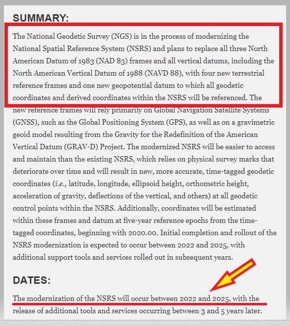
    This column details the potential effects of crustal movement on published heights in various regions of the United States.

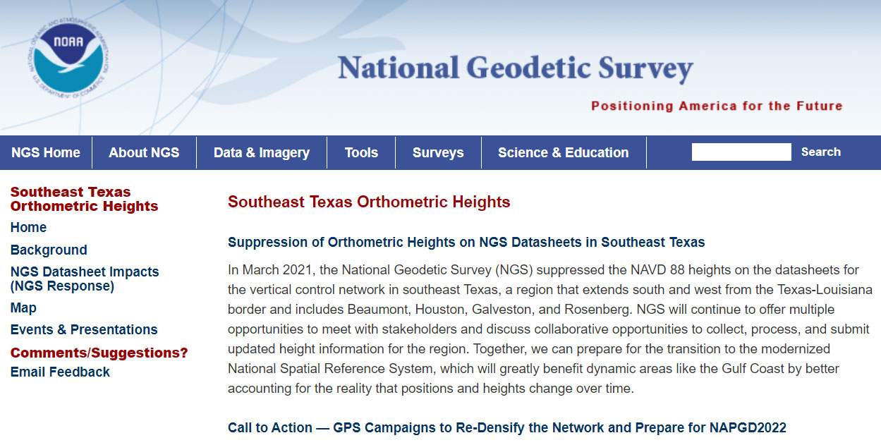
    In my last column (in the April 2021 Survey Scene), I mentioned that the National Geodetic Survey (NGS) announced that it is suppressing height information in Southeast Texas.

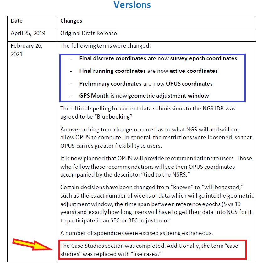
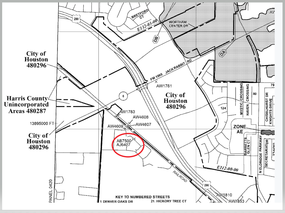
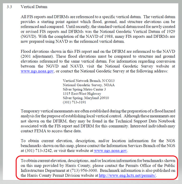
    The April column also highlighted one of NGS’ four use cases – “Use Case 1: Flood Mapping.” The case study discusses the Elevation Certificate (CE) Example, Flood Insurance Rate Map (FIRM) and Flood Insurance Study (FIS).

    The column highlighted the potential effects of subsidence on published heights in the Houston region, which implied that most of the published heights that are based on older surveys in the region are not current or accurate.

    This column will provide more details of the suppression of heights in the Southeast Texas region, and potential effects of crustal movement on published heights in other regions of the United States.

    NGS announcement to suppress height information for Southeast Texas. (Image: NGS)
    NGS announcement that it suppressed height information for Southeast Texas. (Image: NGS)

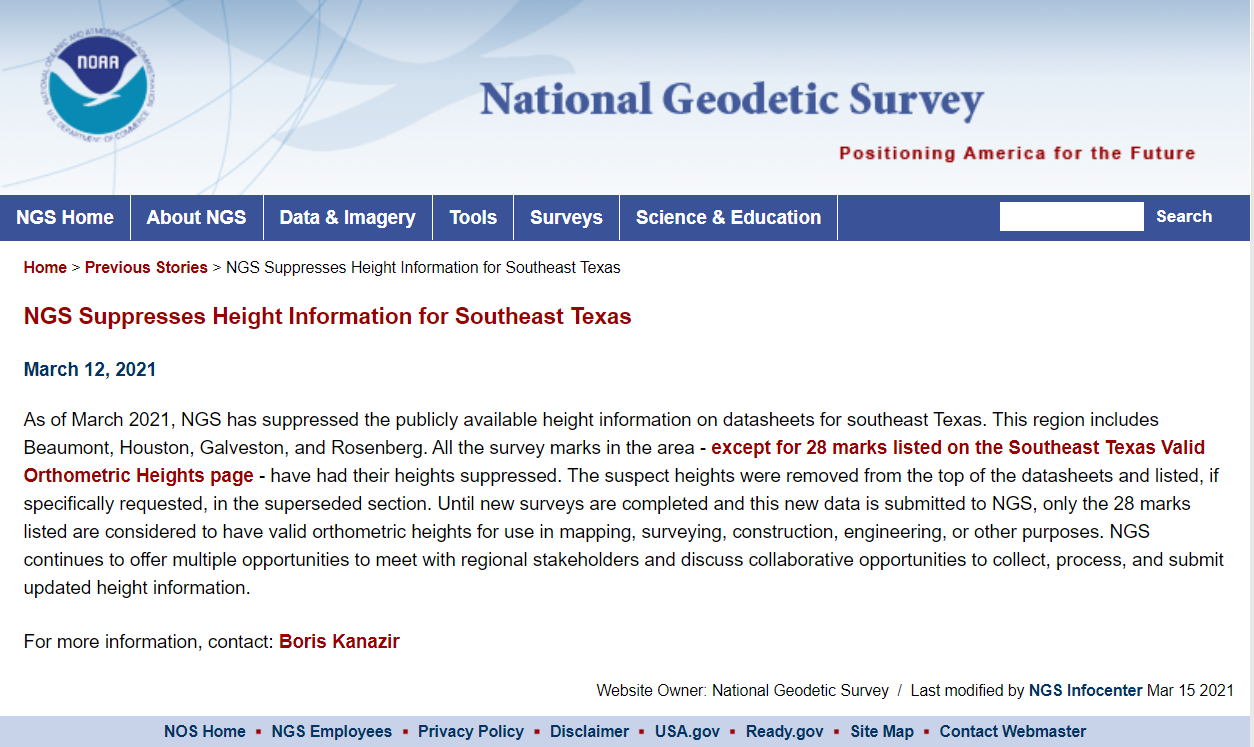
    According to NGS’ announcement, only 28 marks will have publicly available orthometric heights on NGS datasheets in Southeast Texas.

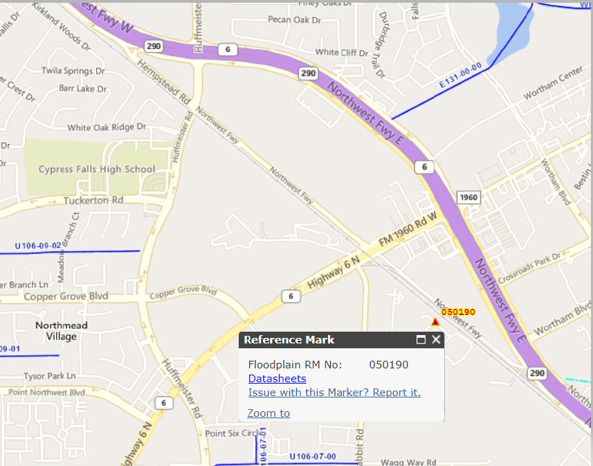
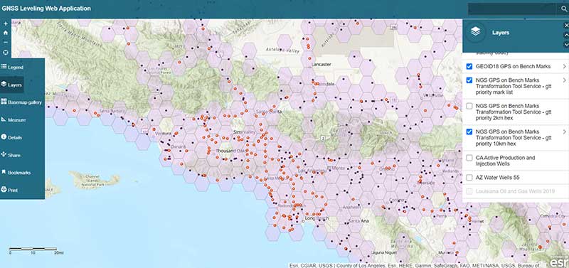
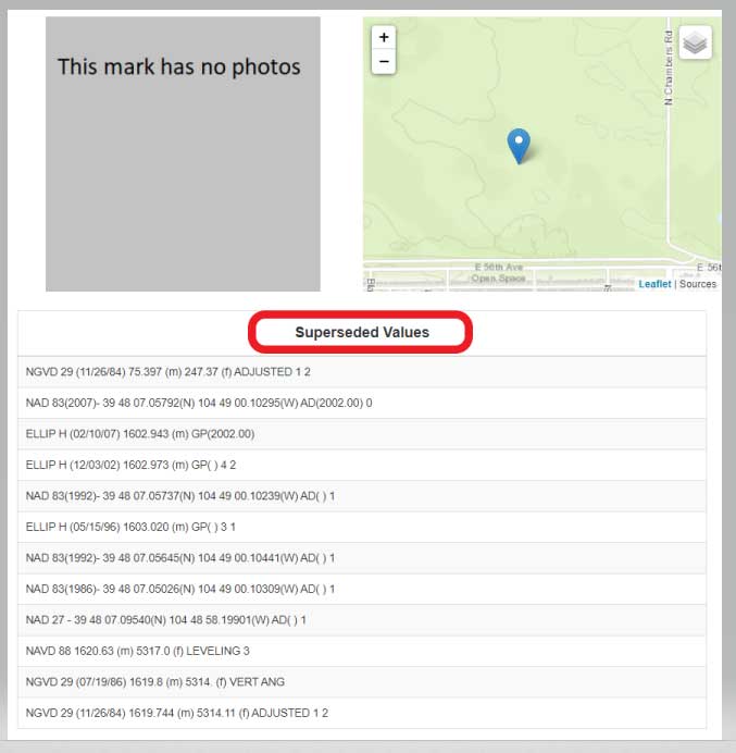
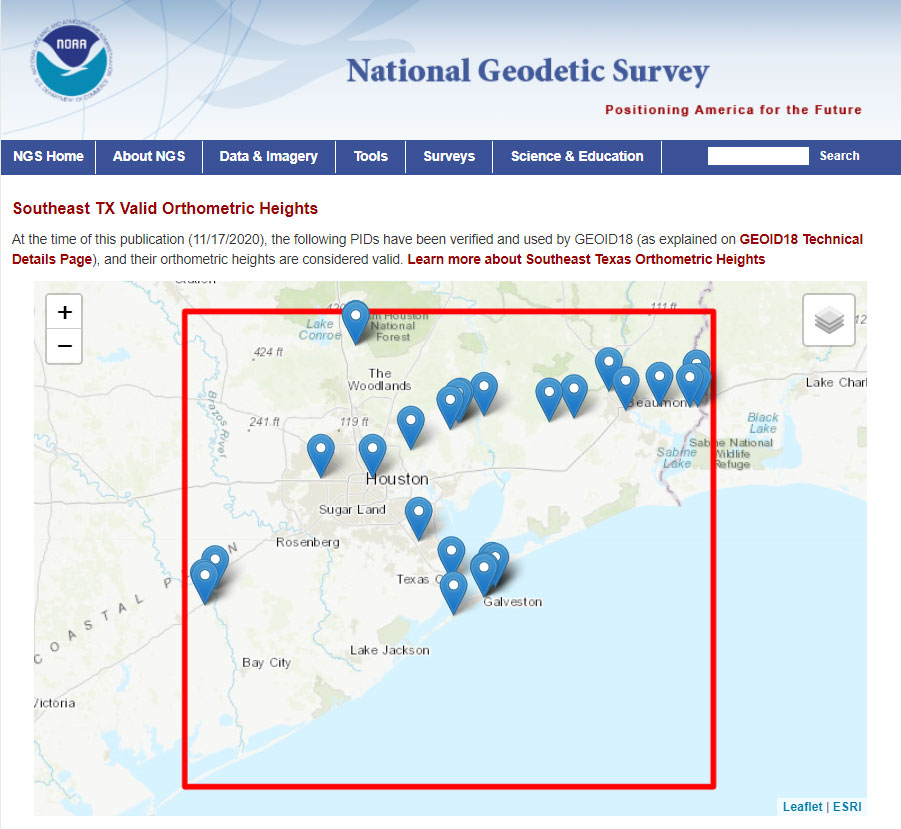
    The “Link to Map: SE TX Valid Ortho. Heights” button provides the benchmarks available to users (see the box titled “Link to Map SE TX Valid Ortho Heights”). The website provides links to the published stations.

    Link to Map SE TX Valid Ortho Heights. (Image: NGS website)
    Link to Map SE TX Valid Ortho Heights. (Image: NGS website)

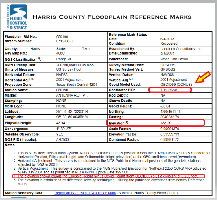
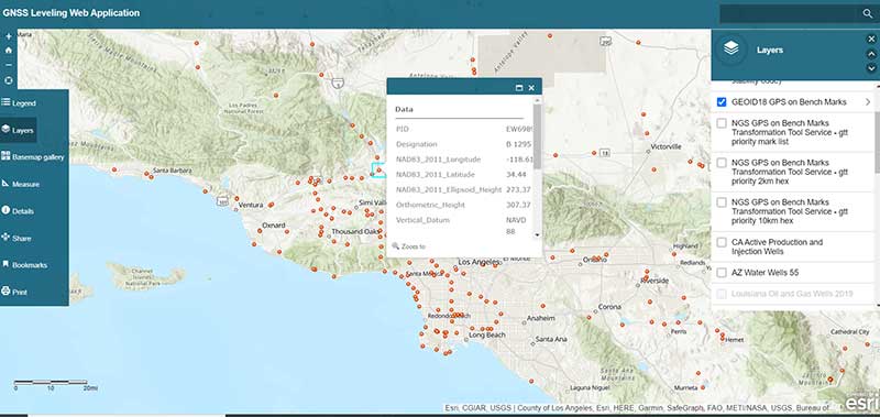
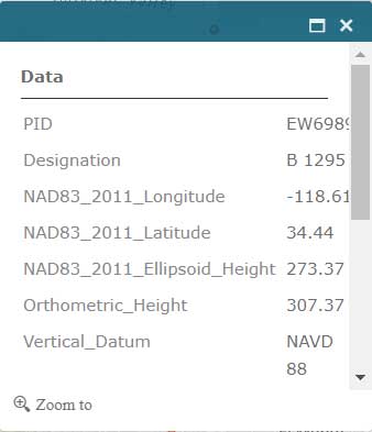
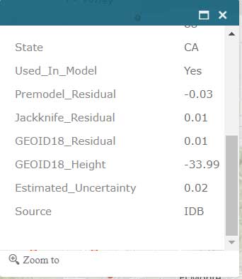
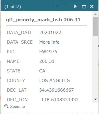
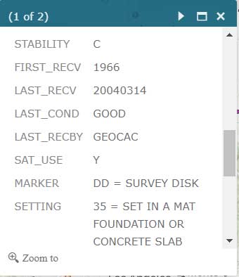
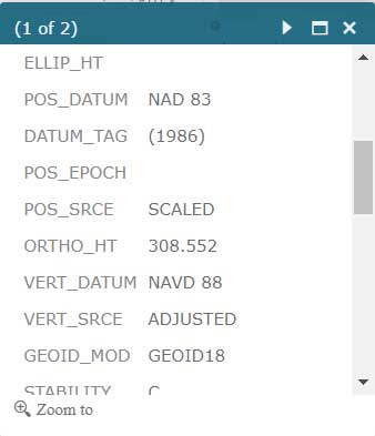
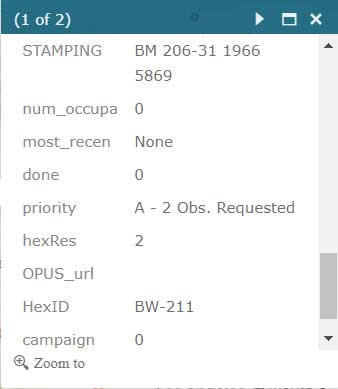
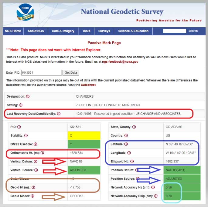
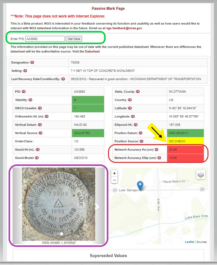
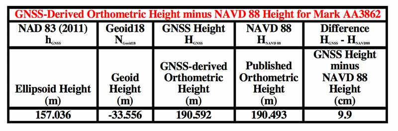
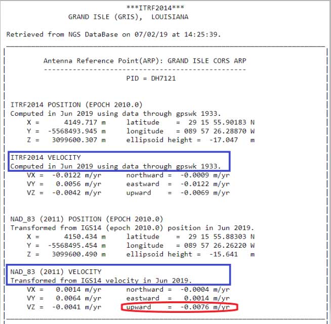
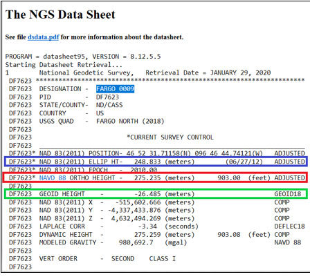
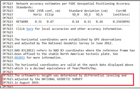
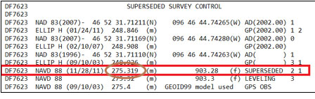
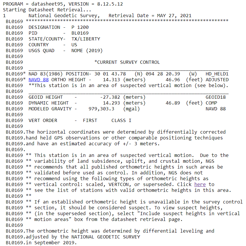
    Clicking on an icon provides the PID and name of the station with a link to a datasheet. Click  “Get Datasheet” for a datasheet of the station. Below is an excerpt from the datasheet of Station P 1200.

    Excerpt from Datasheet of Station P 1200.(Image: NGS Website)
    Excerpt from Datasheet of Station P 1200.(Image: NGS Website)

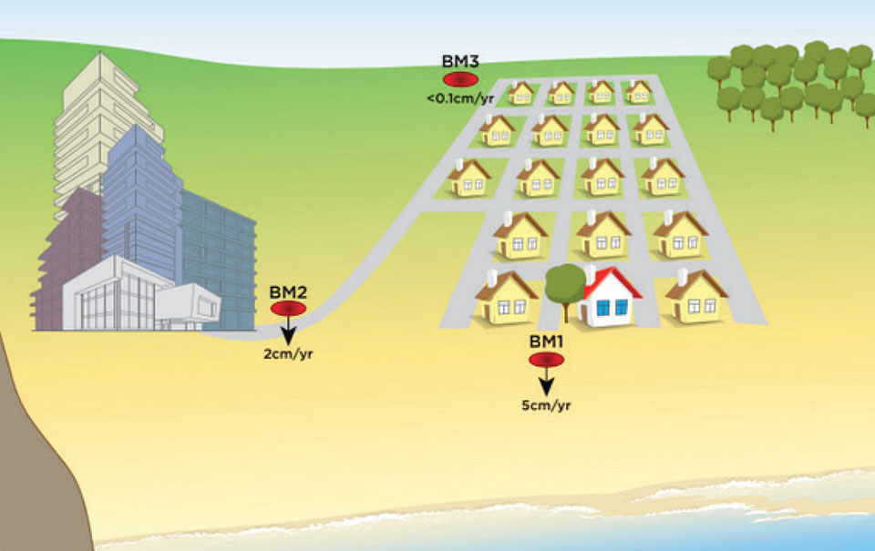
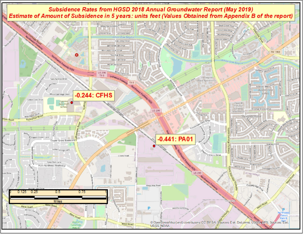
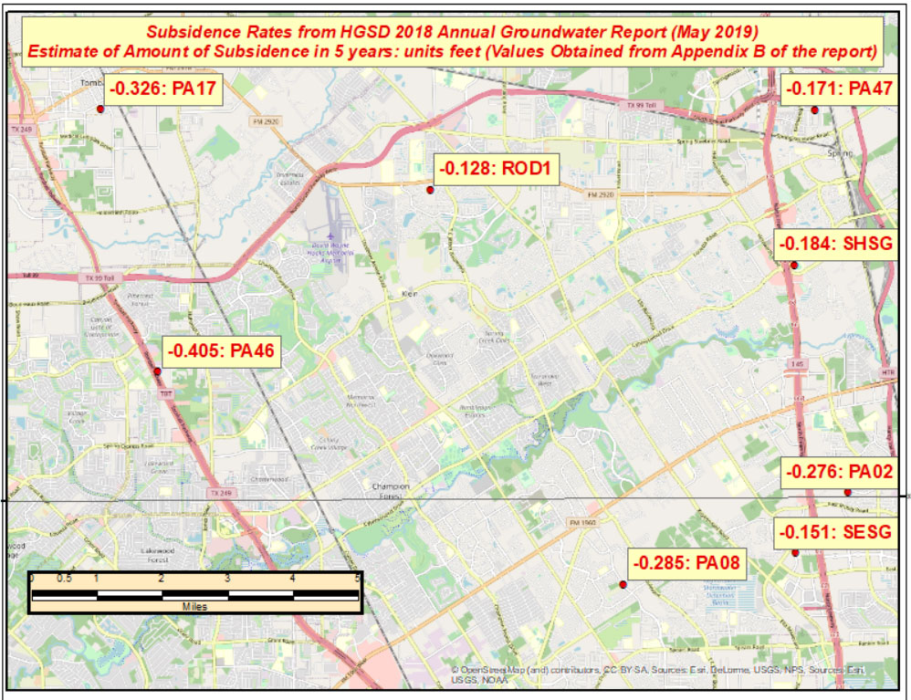
    Let’s address why NGS is suppressing the stations in Southeast Texas. My last column provided plots depicting the amount of movement in the Harris-Galveston, Texas, region. See the box titled “Estimate of Amount of Subsidence in 5 Years in Harris-Galveston, Texas, Region – Units Feet.”

    As indicated in the plot, some of the marks are estimated to have moved almost ½ foot (approximately 0.15 meters) in 5 years. In addition, some of the relative height differences approach 1/3 of a foot (approximately 0.1 meter) between neighboring stations. See the highlighted stations in the box titled “Estimate of Amount of Subsidence in 5 Years in Harris-Galveston, Texas, Region – Units Feet.”

    Estimate of Amount of Subsidence in 5 Years in the Harris-Galveston, Texas, Region – Units Feet. (Image: David Zilkoski)
    Estimate of Amount of Subsidence in 5 Years in the Harris-Galveston, Texas, Region – Units Feet. (Image: David Zilkoski)

    The last major releveling incorporated into NGS’ Database in the Harris-Galveston, Texas, region was performed more than 30 years ago in the 1986/1987 timeframe. Therefore, some of the published stations in the region could have subsided more than three feet (or about a meter).

    As stated in NGS’ Blueprint 3, “Most leveling data in NGS archives comes from the mid-20th century, in support of the NAVD 88 project.” Of course, most regions of the United States are not subsiding at the same rates as in the Houston-Galveston, Texas, region.

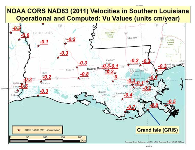
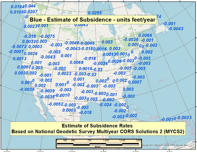
    In a previous newsletter, I discussed NGS’ second Multi-Year CORS Solution of the National CORS (MYCS2). I downloaded the coordinates and velocities from NGS’ website and created a plot of the vertical velocities. For those who prefer to use feet as opposed to meters, I provided velocities with units in feet/year and mm/year.

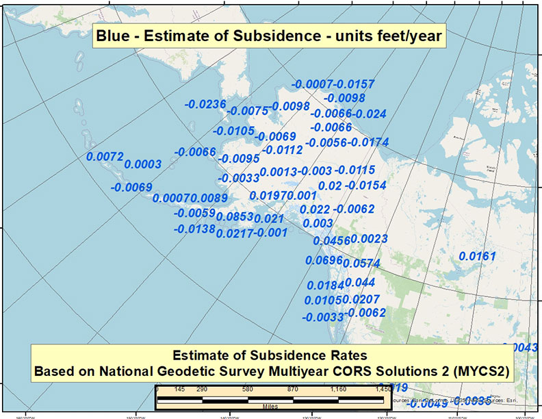
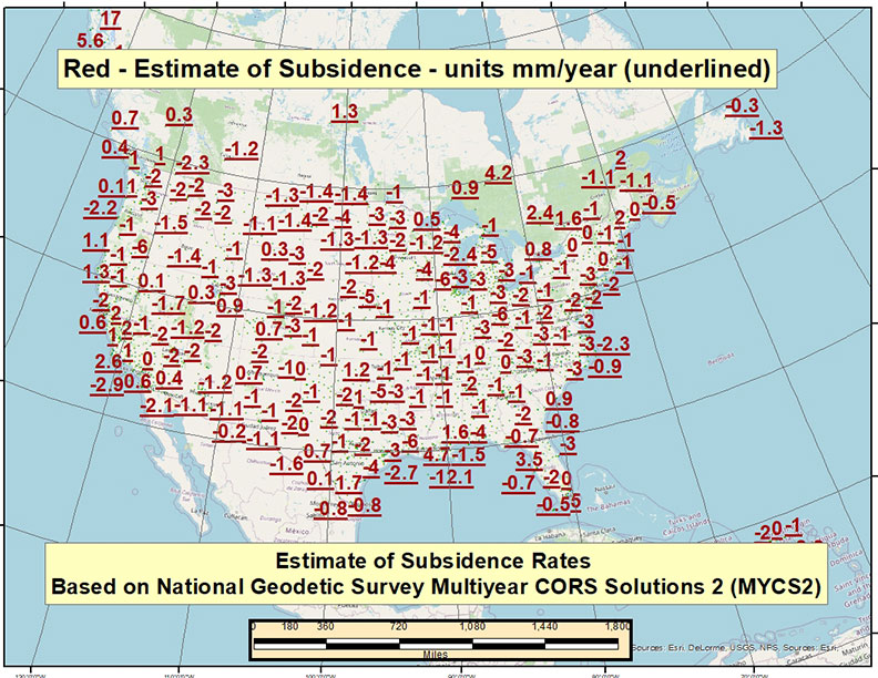
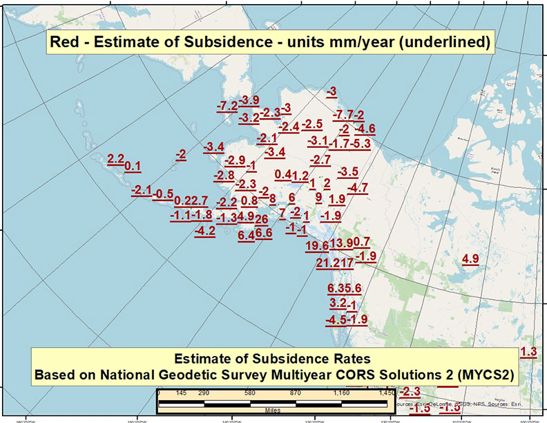
    See the boxes titled “Estimate of Velocity Rates Based on MYCS2 – CONUS (feet/year),” “Estimate of Velocity Rates Based on MYCS2 – Alaska (feet/year),” “Estimate of Velocity Rates Based on MYCS2 – CONUS (mm/year)” and “Estimate of Velocity Rates Based on MYCS2 – Alaska (mm/year).”

    It should be noted that the intent of these four plots is to provide a wide-ranging view of the values and some of the variation in rates across the United States.

    Estimate of Velocity Rates Based on MYCS2 – CONUS (feet/year). (Image: David Zilkoski)
    Estimate of Velocity Rates Based on MYCS2 – CONUS (feet/year). (Image: David Zilkoski)
    Estimate of Velocity Rates Based on MYCS2 – CONUS (feet/year). (Image: David Zilkoski)
    Estimate of Velocity Rates Based on MYCS2 – CONUS (feet/year). (Image: David Zilkoski)
    Estimate of Velocity Rates Based on MYCS2 – CONUS (mm/year). (Image: David Zilkoski)
    Estimate of Velocity Rates Based on MYCS2 – CONUS (mm/year). (Image: David Zilkoski)
    Estimate of Velocity Rates Based on MYCS2 – Alaska (mm/year). (Image: David Zilkoski)
    Estimate of Velocity Rates Based on MYCS2 – Alaska (mm/year). (Image: David Zilkoski)

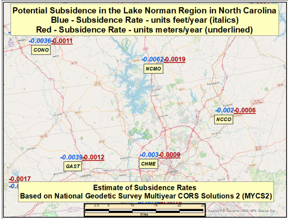
    The rates appear to be small in most regions of the United States. As an example, the rates are all less than -0.0062 feet/year (-0.0019 meters/year) in the Lake Norman region in North Carolina (see the box titled “Potential Subsidence Rates in the Lake Norman Region in North Carolina). It would take many years for the crustal movement to make a difference to some projects in this region.

    Potential Subsidence Rates in the Lake Norman Region in North Carolina. (Image: David Zilkoski)
    Potential Subsidence Rates in the Lake Norman Region in North Carolina. (Image: David Zilkoski)

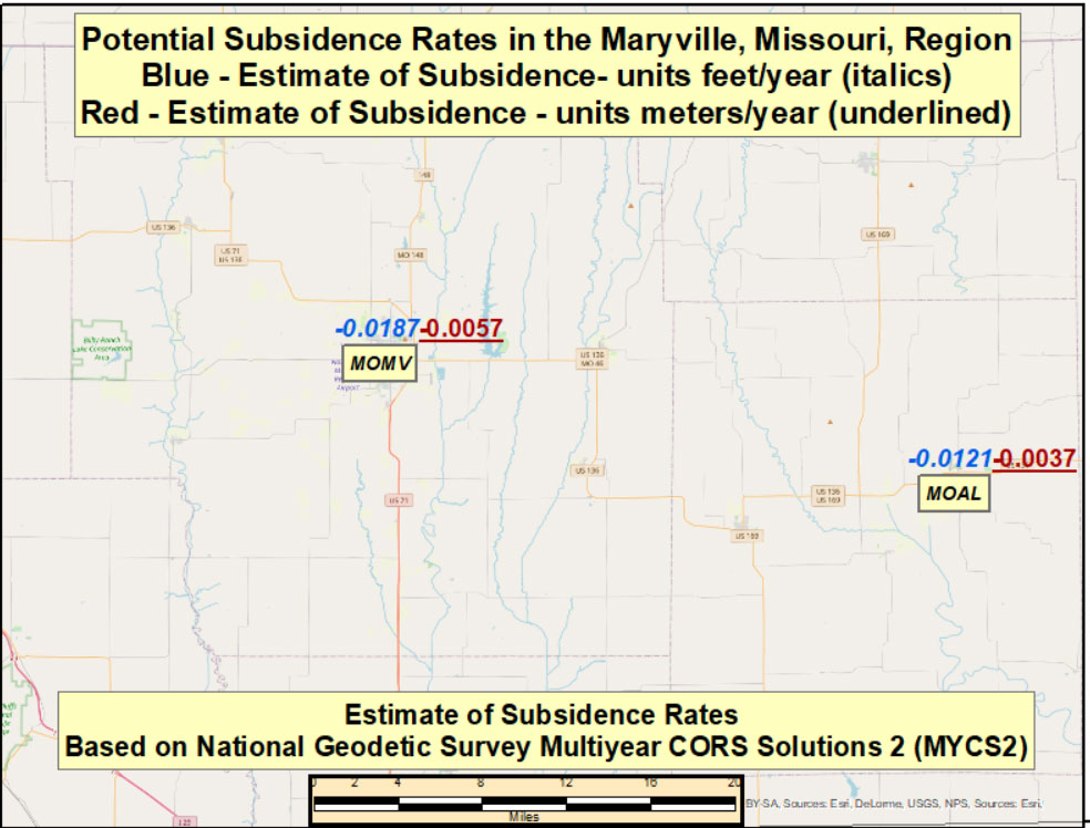
    That said, let’s look at another region of the country. For example, in the vicinity of Maryville, Missouri, the rate of subsidence is around -0.0187 feet/year (-0.0057 meters/year). See the box titled “Potential Subsidence Rates in the Maryville, Missouri, Region.” These subsidence rates don’t appear to be large values but if you take into account the last time the height of a mark was established by leveling data it could result in a large difference from the true orthometric height.

    Potential Subsidence Rates in the Maryville, Missouri, Region. (Image: David Zilkoski)
    Potential Subsidence Rates in the Maryville, Missouri, Region. (Image: David Zilkoski)

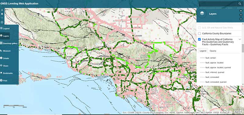
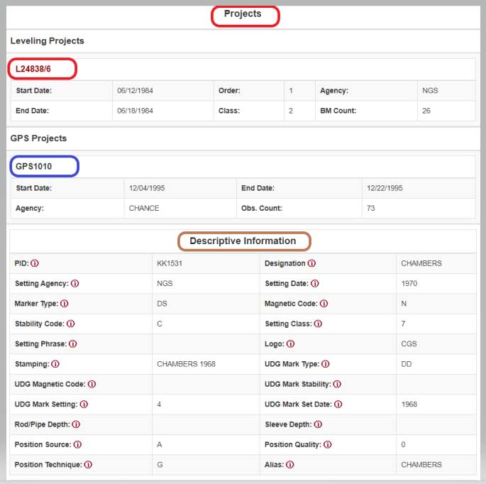
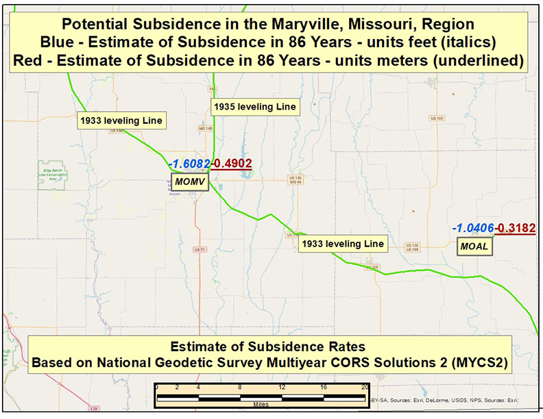
    According to NGS’ database, it appears that many of the marks in the Maryville, Missouri, region were last leveled in 1935. I used NGS’ Passive Mark Lookup tool and Leveling Project Page tool to identify the marks and associated leveling lines in the area of the CORS stations in the Maryville, Missouri, region.

    I described the Passive Mark Lookup webtool in a previous column. As previously mentioned, these subsidence rates all seem very small, but if you take into account the last time the height of mark was established by leveling data, the subsidence value can be very large.

    See the box titled “Potential Subsidence in 86 Years in the Maryville, Missouri, Region.” The box indicates that, if you account for the last 86 years (2021 – 1935), the potential subsidence exceeds 1½ feet (-1.6082 feet, -0.4902 meters).

    Potential Subsidence in 86 Years in the Maryville, Missouri, Region. (Image: David Zilkoski)
    Potential Subsidence in 86 Years in the Maryville, Missouri, Region. (Image: David Zilkoski)

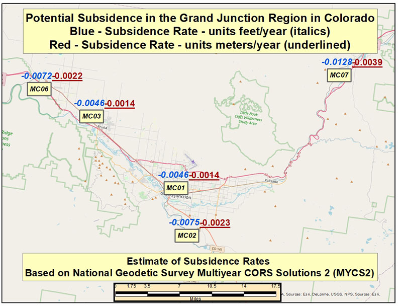
    Continuing across the country to Colorado, the box titled “Potential Subsidence Rates in the Grand Junction Region, Colorado,” provides the estimate of subsidence rates in Mesa County, Colorado. As the plot indicates, the rates vary between -0.0046 feet/year (-1.4 mm/year) and -0.0128 feet/year (-3.9 mm/year). Once again, these rates all seem relatively small but many of the marks near CORS MC06 were last leveled in 1985. This means the potential change in height could be as large as 0.2592 feet (0.0792 meters).

    Potential Subsidence Rates in the Grand Junction. Colorado, Region. (Image: David Zilkoski)
    Potential Subsidence Rates in the Grand Junction Region, Colorado. (Image: David Zilkoski)

    Obviously, this is only an estimate of the subsidence in the region and the actual amount of subsidence is unknown since the last time the mark was leveled. These estimates are based on the MYCS2, which uses current data to estimate the velocity. The processing included data spanning 1996 to 2016 (week 0834 to 1933), 1099 weeks or about 21 years in total.

    The point of this column is not to provide the exact change in height of a mark, but to highlight that the publicly available orthometric height on a NGS datasheet may not be up to date based on crustal movement. The new modernized National Spatial Reference System will enable users to determine an accurate, current height on a mark and be able to efficiently and effectively monitor changes in a mark’s height.

    As stated in NGS’ announcement to suppress the heights in Southeast Texas, the agency has developed tools to assist users in submitted data to NGS. See the box titled “Excerpt from NGS Announcement to Suppresses Height Information for Southeast Texas.”

    Excerpt from NGS Announcement to Suppresses Height Information for Southeast Texas. (Image: NGS website)

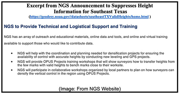
    This assistance is for every user, not just for individuals performing surveys in Southeast Texas. NGS has Regional Geodetic Advisors throughout the United States.

    NGS Regional Geodetic Advisors. (Image: NGS Website)
    NGS Regional Geodetic Advisors. (Image: NGS Website)

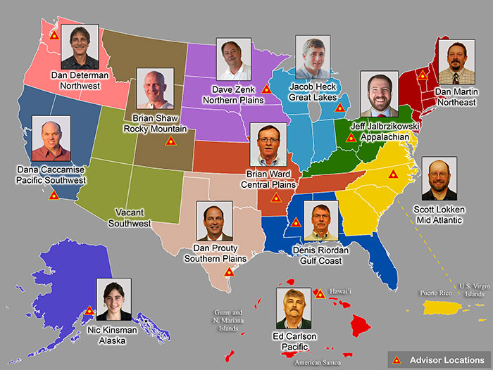
    The Regional Geodetic Advisors provide guidance and assistance to constituents within their region. They are subject-matter experts in geodesy and regional geodetic issues. These individuals can assist users that are planning GNSS campaigns to re-densify the network.

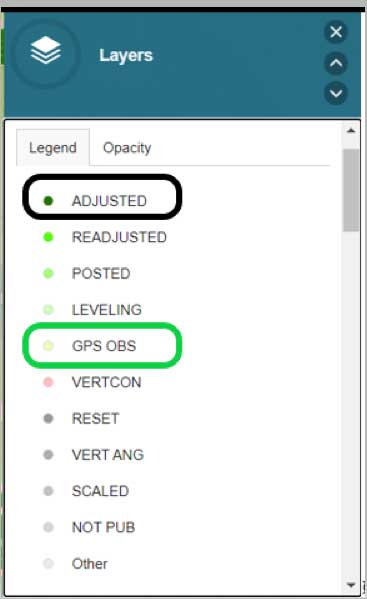
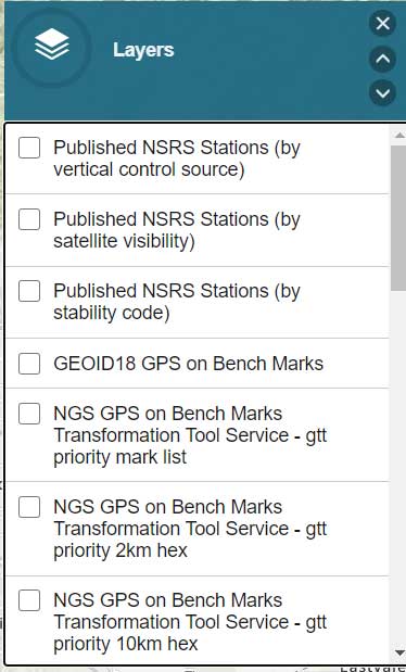
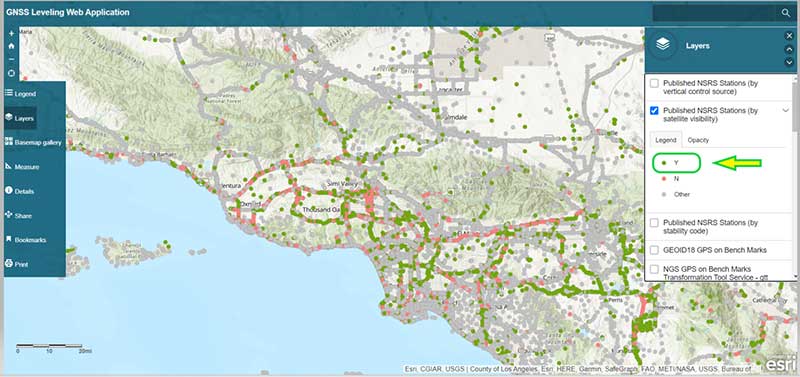
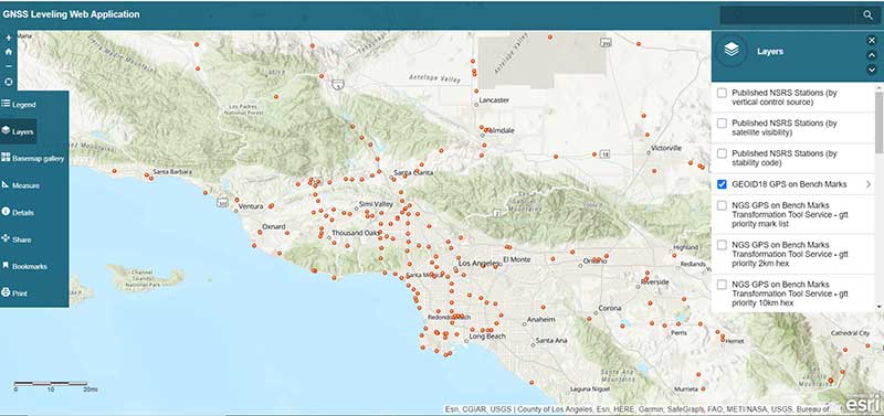
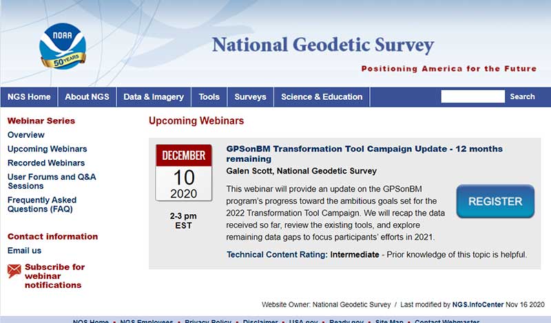
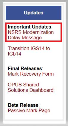
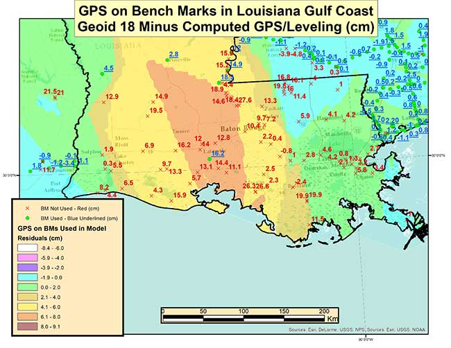
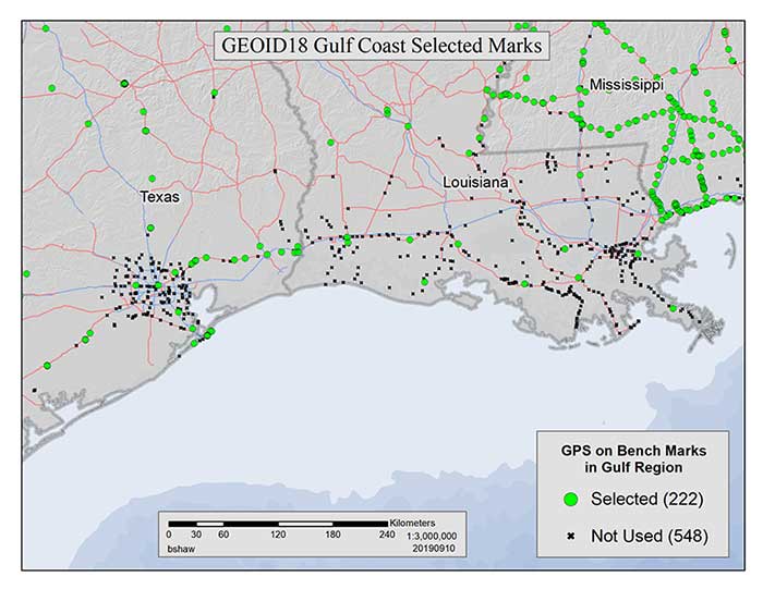
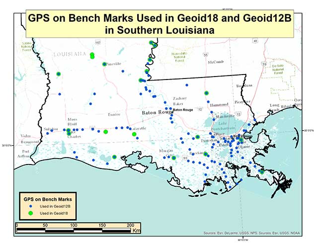
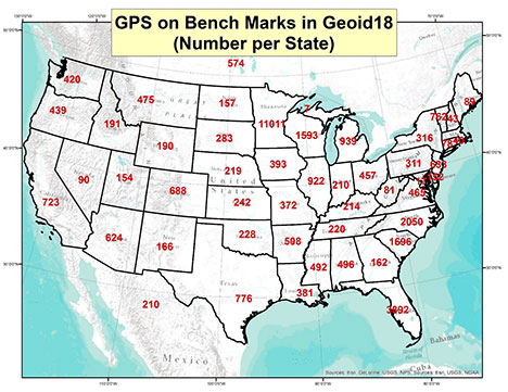
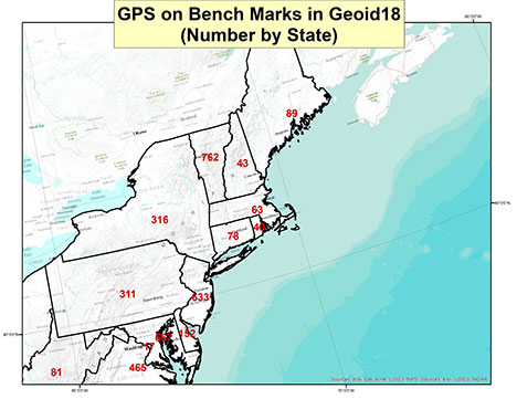
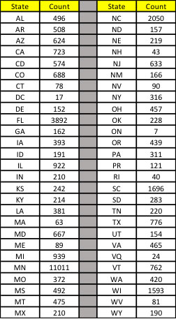
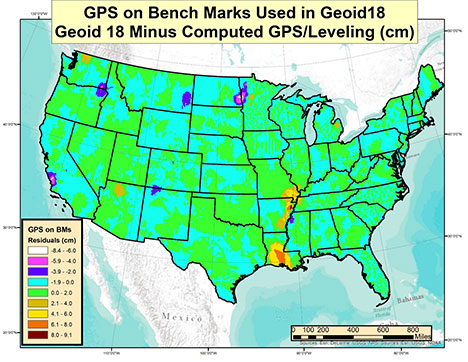
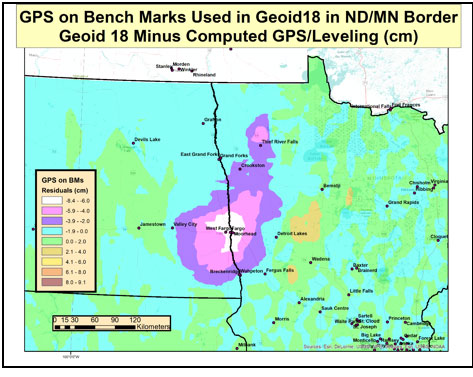
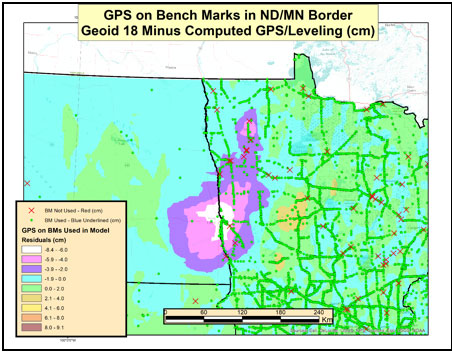
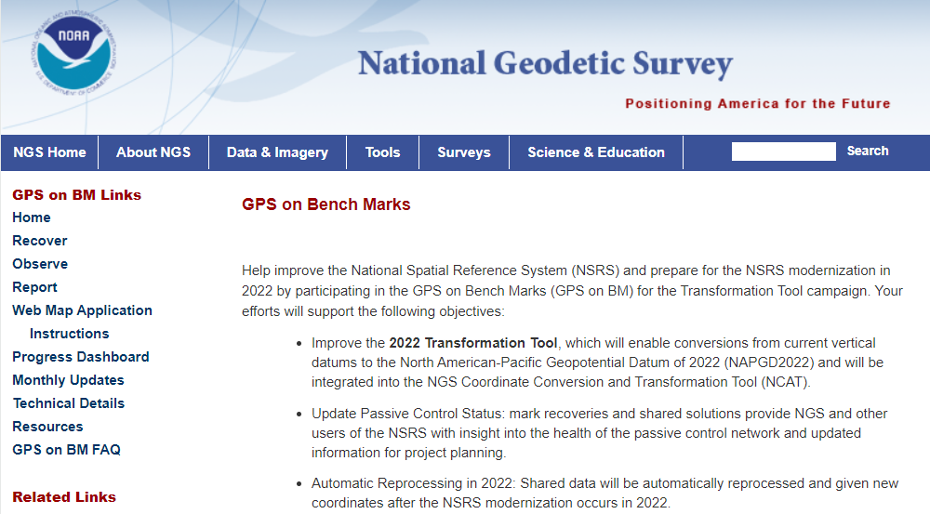
    NGS also provides a website detailing how users can help densify the network to prepare for the new, modernized North American-Pacific Geopotential Datum of 2022 (NAPGD2022). See the box titled “NGS GPS on Bench Marks Webpage.”

    As mentioned in previous newsletters, a benefit of the new modernized National Spatial Reference System (NSRS) will facilitate the establishment of consistent, accurate NAPGD2022 GNSS-derived orthometric heights.

    NGS GPS on Bench Marks webpage. (Image: NGS Website)
    NGS GPS on Bench Marks webpage. (Image: NGS Website)

    This column provided details on the suppression of heights in the Southeast Texas region, and potential effects of crustal movement on published heights in other regions of the United States. NGS suppressed the heights in the Southeast Texas region because of the large amount of crustal movement since the last time the heights of the marks were established.

    As indicated by NGS’ MYCS2 velocities, every mark could be affected by crustal movement. In my opinion, the question a user should be asking is “How much has the height of the mark changed since it was last determined? Not, “Has the height of the mark changed?”

  • NGS revises NOAA report on working in the modernized NSRS

    NGS revises NOAA report on working in the modernized NSRS

    The National Geodetic Survey (NGS) has revised an important technical document on the modernized National Spatial Reference System (NSRS). Zilkoski explores a use case on flood mapping, discussing an Elevation Certificate example, Flood Insurance Rate Map and Flood Insurance Study. NGS has scheduled a webinar for April 8 to discuss the four use case examples. 

    In February 2021, the National Geodetic Survey (NGS) revised NOAA Technical Report NOS NGS 67 Blueprint for the Modernized NSRS, Part 3: Working in the Modernized NSRS. Users can download the publication. See the box titled “NOAA Technical Report NOS NGS 67.”

    NOAA Technical Report NOS NGS 67.(Image:NGS)
    NOAA Technical Report NOS NGS 67. (Image: NGS)

    On March 11, NGS held a webinar describing the revised document (see box titled “Working in the Modernized NSRS”). Download a video of the webinar and the presentation.

    Working in the Modernized NSRS. (Image: NGS}
    Working in the Modernized NSRS. (Image: NGS}

    The revised document added four use cases to describe how someone might access and use the NSRS in the future:

    • Use Case 1: Flood Mapping,
    • Use Case 2: Passive Control for a Multi-year Corridor Project,
    • Use Case 3: Transitioning Data to the Modernized NSRS, and
    • Use Case 4: Leveraging the Modernized NSRS for Airport and Other Infrastructure Monitoring.

    The box titled “Major Changes to NOS NGS 67” highlights the changes in the February 2021 revised version.

    Major Changes to NOS NGS 67. (Image: NGS)
    Major Changes to NOS NGS 67. (Image: NGS)

    This column will highlight one of the four use cases:  “Use Case 1: Flood Mapping.” The case study discusses the Elevation Certificate (CE) example, Flood Insurance Rate Map (FIRM), and Flood Insurance Study (FIS).

    The following is the scenario that NGS considered in this use case:

    “This use case’s examples are set in an imaginary flood-prone coastal community experiencing non-uniform ground subsidence at the watershed scale (see Figure 10). Although many areas are not subject to this level of vertical motion, the full benefits of NSRS modernization are most apparent in this context. We illustrate differences in the use of the NSRS of today and the modernized NSRS with two common NFIP workflows. First, we consider steps anticipated in the certification of NAPGD2022 elevations for a NFIP Elevation Certificate. Second, we step into the shoes of a FEMA Mapping Partner to examine the ways future NSRS tools support more accurate mapping in Flood Insurance Rate Map (FIRM) and Flood Information Study (FIS) updates.”

    I think this is a good scenario to use to demonstrate the full benefits of the NSRS modernization in areas of subsidence, but I believe there are important issues that will need to be addressed before the implementation of NAPGD2022 in flood mapping projects. I will highlight some of these issues later in the newsletter. First, let’s look at NGS example.

    As depicted in figure 10 in NOS NGS 67 technical document, the area has three difference subsidence rates (<0.1 cm/yr., 2 cm/yr., and 5 cm/yr.). See the box titled “Diagram of fictional case study location for Use Case 1.” As NGS stated in the document, “Although many areas are not subject to this level of vertical motion, the full benefits of NSRS modernization are most apparent in this context.”

    This may not be the typical situation of a flood mapping project but it should be noted that this type of high individual rates and large relative rate differences has occurred in the Houston-Galveston, Texas, region (see the following publications):

    NGS’s example illustrates differences in the use of the NSRS today and the future NSRS with two common National Flood Insurance Program (NFIP) workflows. The example addresses surveyors performing a FEMA Elevation Certification using NAPGD2022 elevations, and the ways future NSRS tools support more accurate mapping in Flood Insurance Rate Map (FIRM) and Flood Information Study (FIS) updates.

    Figure 10 from NOAA Technical Report NOS NGS 67 — Diagram of fictional case study location. The arrows correspond to hypothetical rates of ground subsidence. (Image: NGS)
    Diagram of fictional case study location for Use Case 1 (Figure 10), The arrows correspond to hypothetical rates of ground subsidence. (Image: NGS)

    It should be noted that according to the September 27, 2017, Office of Inspector General Department of Homeland Security OIG-17-110 report, FEMA’s goal is to review flood maps every five years.

    “According to the National Flood Insurance Reform Act of 1994, FEMA must assess the need to revise and update all floodplain areas and flood risk zones identified once during each 5-year period. Thus, valid miles will expire every five years if not assessed. Failure to assess an NVUE compliant mile within the 5-year window will result in the mile being re-categorized as “Unknown” in the Needs Database. Unknown miles have not been subjected to the validation process to determine whether they reflect the current flood risk or are in need of restudy. In 2009, FEMA set a goal to attain 80 percent NVUE by the end of fiscal year 2014.” — Excerpt from Department of Homeland Security OIG-17-110 report

    The modernized NSRS will help facilitate meeting this goal. This is described in NGS’s use case example:

    NFIP products will primarily utilize the official NSRS reference epochs

    “As the NFIP is structured today, NFIP products will primarily utilize the official NSRS reference epochs. Additionally, some NFIP products such as the EC form itself, as well as guidance, and technical references for FIRM and FIS preparation would benefit from updates that reflect changes to the NSRS. While the time-dependency and incorporation of a gravimetric geoid model will manifest as improved risk assessment reliability in inundation map products, we notably anticipate that NSRS modernization will have a limited impact on the basic structure of most recommended workflows associated with the NFIP of today. The most significant development is therefore the opportunity for FEMA’s National Flood Mapping Program (NFMP) to increasingly leverage the new capabilities of the NSRS to ensure that current, accurate ground elevation data is used, and to better incorporate relevant flood control structure and future conditions mapping data to support decision-making beyond the NFIP. Details of how the modernized NSRS can help FEMA achieve broader NFMP objectives and opportunities for data-driven case studies to explore this are described at the end of the use case.”

    So, what does this really mean? The document uses two diagrams to explain how the new NSRS would be used to estimate a height for a FEMA Elevation Certificate (see box titled “Figure 11 from Use Case 1”). The top cartoon labeled “Tie to Passive Control” describes the process being performed today. That is, a surveyor locates the two closest marks that have published orthometric heights, follows the appropriate surveying procedures to ensure that the marks have not moved since the last time they were leveled to, and then performs the appropriate procedures to obtain the height for the Elevation Certificate. Depending on the location of the published orthometric heights in the area of the structure, this process could be very expensive. The lower cartoon labeled “Tie to Active Control” describes the process that will be used in the modernized NSRS using NADGP2022 heights. The user would occupy a temporary mark near the structure with GNSS to obtain a NAPGD2022 orthometric height computed using the appropriate ellipsoid height and geoid height value, and then perform the appropriate leveling procedures to obtain the height for the Elevation Certificate. This process will provide the most up-to-date height in the area.

    Figure 11. Cartoon of Elevation Certificate field surveys based on establishing a tie to the NSRS via passive control leveling (top panel) and via active control with GNSS (lower panel). (Image: NGS)
    Figure 11 from Use Case 1. Cartoon of Elevation Certificate field surveys based on establishing a tie to the NSRS via passive control leveling (top panel) and via active control with GNSS (lower panel). (Image: NGS)

    There is an issue that should be noted here: the temporary mark determined using active control may provide the most up-to-date height at a particular location but that height may not be consistent with the heights used to establish the Base Flood Elevation (BFE). At first, someone would say, that’s good because it’s indicating that the flood hydraulics have changed on the floodplain map. However, without performing a detailed height analysis in the region, the user won’t really know whether the BFE value should be updated based on the current changes in topography in the floodplain region. In other words, if the entire region has subsidence at the same rate then the relative height difference hasn’t changed, and the new starting height may not be consistent with the published BFE on the FEMA Floodplain Map. In most floodplain mapping regions, the changes in heights are probably less than the accuracy of the maps but using the height of a mark that is not consistent with the BFE could place a homeowner’s house incorrectly in a flood zone. A good surveying practice would include occupying several marks with GNSS (or leveling between marks) that were involved in the creation of the flood insurance study and the generation of the floodplain map to ensure that the height used on the Elevation Certificate is consistent with the BFE. This is a good procedure to use for the current NSRS as well as the modernized NSRS. However, this is not economically practical using the current NSRS but could be in the new NSRS which is a major benefit of the modernized NSRS.
    So, let’s look at the Houston-Galveston region using the latest information available.

    Download latest FEMA Flood Insurance Rate Map (FIRM). See box titled “Excerpt from FEMA FIRM Map Number 48201C0440N.”

    Excerpt from FEMA FIRM Map Number 48201C0440N. (Image: FEMA)
    Excerpt from FEMA FIRM Map Number 48201C0440N. (Image: FEMA)

    According to the latest Flood Insurance Study (FIS), the heights used in the study were based on a 2001 adjustment performed by the county. You can download the FIS from FEMA Flood Map Service Center | Search All Products, 48201CV001G (fema.gov) and map1.msc.fema.gov.

    I’d like to highlight a few statements in the FIS. First, the reports states that the FIS and DFIRM are referenced to the NAVD (2001 Adjustment). See the box titled “Page 111 from November 15, 2019 Flood Insurance Study 48201CV001G.” The report provides a link for users to obtain the latest vertical control data. Users can find information about the Harris County Floodplain Reference Marks here (See box titled “Harris County Floodplain Reference Marks.”) Users also can access the vertical control data at the county website.

    Page 111 from Nov. 15, 2019, Flood Insurance Study 48201CV001G. (Image: FEMA)
    Page 111 from Nov. 15, 2019, Flood Insurance Study 48201CV001G. (Image: FEMA)
    Harris County Floodplain Reference Marks. (Image: Harris County Flood Control District)
    Harris County Floodplain Reference Marks. (Image: Harris County Flood Control District)

    The box titled “Snapshot of Vertical Control from Harris County Floodplain Reference Marks Website” depicts the location of one of the reference marks, denoted as 050190.

    Snapshot of Vertical Control from Harris County Floodplain Reference Marks Website. (Image: (Image: Harris County Flood Control District))
    Snapshot of Vertical Control from Harris County Floodplain Reference Marks Website. (Image: Harris County Flood Control District))

    Clicking on the datasheets link, provides the information about the floodplain reference mark in the Harris County Flood Control District’s system (see the box titled “Harris County Floodplain Reference Mark Datasheet”).

    Harris County Floodplain Reference Mark Datasheet. (Image: Harris County Flood Control District)
    Harris County Floodplain Reference Mark Datasheet. (Image: Harris County Flood Control District)

    It should be noted that the GNSS-derived orthometric heights were based on GEOID99 and the official hybrid geoid model published by NGS today is GEOID18. A GNSS-derived orthometric height computed using NGS’ webtool OPUS will use GEOID18 not GEOID99. The difference between GEOID99 and GEOID18 at this location is approximately 0.45 feet (0.138 meters). Users must ensure that they are using heights that are consistent with the BFE on the FIRM. The new NAPGD2022 will help to reduce issues associated with effects due to changes in geoid models.

    Page 113 from the November 15, 2019 Flood Insurance Study 48201CV001G addresses the issues associated with riverine flood in the region. (See the box titled “Page 113 from November 15, 2019 Flood Insurance Study 48201CV001G.”) The highlighted sections basically state that subsidence within inland watersheds has little or no effect on flood depths when the entire watershed subsides at the same rate. However, it also states that differential subsidence can cause changes in flood depths. The report goes on to say that the “Harris County and Incorporated Areas are affected by wide-scale, uniform subsidence with minor differential subsidence within individual watersheds.” It also states that “The local effects of subsidence may be adequately addressed, in the short term, by assuming that BFEs subside by the same amount the ground subsides.” The Houston-Galveston, Texas, region is a very complicated area due to the differential subsidence and numerous individual watersheds.

    Page 113 from November 15, 2019 Flood Insurance Study 48201CV001G. (Image: FEMA)
    Page 113 from November 15, 2019, Flood Insurance Study 48201CV001G. (Image: FEMA)

    That said, let’s look some of the latest subsidence data in the region. The Harris-Galveston Subsidence District’s 2018 Annual Groundwater Report By Robert Thompson, William M. Chrismer, and Christina Petersen, PhD, P.E. provide some of the latest estimates of subsidence in the region. The box titled “HGSD Exhibit 18” depicts the locations of the GNSS sites used in the study. The plot provides the average compaction in centimeters over the past five years. The values range from 0.0 cm/year to greater than 2.5 cm/year.

    HGSD Exhibit 18. (Image: Harris-Galveston Subsidence District)
    HGSD Exhibit 18. This map shows the locations of the GPS sites throughout the area. The colored dots represent the average compaction over the past five years for each site, in centimeters. They range from 0.0 cm/year to greater than 2.5 cm/year. (Image: Harris-Galveston Subsidence District)

    I used the information from Appendix B provided in the report to generate a few plots that show the estimate of subsidence in feet over 5 years. I’ve highlighted some marks that have large relative height changes. (Note: The units of the previous figure are centimeters; the units of the next several plots are feet.)

    Estimate of Amount of Subsidence in 5 Years – Units: Feet. (Image: David Ziljoski)
    Estimate of Amount of Subsidence in 5 Years – Units: Feet. (Image: David Zilkoski)

    The relative height change between the two marks PA01 and CFHS, which are about 1.5 kilometers (approximately 1 mile) apart, is 0.197 feet in only 5 years. (See the box titled “Estimate of Amount of Subsidence in 5 Years at Pam 1– Units Feet.”)

    Estimate of Amount of Subsidence in 5 Years at Pam 1 – Units: Feet. (Image: David Ziljoski)
    Estimate of Amount of Subsidence in 5 Years at Pam 1 – Units: Feet. (Image: David Zilkoski)

    The estimated relative height change between mark PA46 and ROD1, which are about 8 kilometers (approximately 5 miles) apart, is 0.277 feet in five years. (See the box titled “Estimate of Amount of Subsidence in 5 Years at Pam 46 – Units: Feet.”)

    Estimate of Amount of Subsidence in 5 Years at Pam 46 – Units: Feet. (Image: David Ziljoski)
    Estimate of Amount of Subsidence in 5 Years at Pam 46 – Units: Feet.(Image: David Zilkoski)

    The effect of these large relative differences may not have any effect on the BFE on a particular watershed. These subsidence estimates are at a specific mark so they only provide information at a particular location. The new NAPGD2022 along with NGS’s webtools will enable users to economically obtain current, accurate heights in the entire region. Leveraging the capabilities of the new NSRS will help facilitate the implementation of FEMA’s goal of assessing the need to revise and update all floodplain areas and flood risk zones identified once during each five-year period.

    There’s one last item that I’d like to highlight in this newsletter. On March 12, NGS announced that they are suppressing height information in Southeast Texas. See the box titled “NGS Announcement to Suppresses Height Information for Southeast Texas” for more information.

    This column highlighted the potential effects of subsidence on published heights in the Houston, Texas, region, which implies that most of the published heights based on older surveys in the region are not current or accurate.

    NGS announcement to suppress height information for Southeast Texas. (Image: NGS)
    NGS announcement to suppress height information for Southeast Texas. (Image: NGS)

    According to the announcement, only 28 marks will have publicly available orthometric heights on NGS datasheets in Southeast Texas. This NOAA  website provides more information. See the box titled “NGS Southeast Texas Orthometric Heights.”

    NGS Southeast Texas Orthometric Heights. (Image: NGS)
    NGS Southeast Texas Orthometric Heights. (Image: NGS)

    I would encourage everyone to check out the website to obtain a better understanding of what this suppression of published heights means to their operations. Future newsletters will address the suppression of the orthometric heights in Southeast Texas, and how users can help densify the network and prepare for the new, modernized NAPGD2022. Again, a benefit of the new modernized NSRS will facilitate the establishment of consistent, accurate NAPGD2022 GNSS-derived orthometric heights.

    Lastly, NGS is convening the 2021 Geospatial Summit on May 4 and 5. The 2021 Geospatial Summit will provide updated information about the planned modernization of the National Spatial Reference System (NSRS). Register here.

  • NGS releases annual experimental geoid models and gravity interpolation tools

    NGS releases annual experimental geoid models and gravity interpolation tools

    My last column highlighted an ArcGIS web application that incorporates various datasets and data layers to assist surveyors planning vertical control surveys. On Jan, 29, the National Geodetic Survey (NGS) released the latest experimental geoid model, xGeoid20, and a new gravity interpolation tool (see box below, “NGS Releases Annual e& Gravity Interpolation Tools”).

    This newsletter will highlight some attributes of these two new products. First, why am I writing about another experimental geoid model. I discussed xGeoid18 in my December 2018 column and xGeoid16 in my June 2017 column. What’s important here is that this will be the last experimental geoid model until 2022, and the dynamic geoid model has also been updated this year in the form of xDGEOID20.

    xDGEOID20 is produced by NGS within the Geoid Monitoring Sƒervice (GeMS) and is part of the new NAPGD2022. Therefore, users only have a few more years to understand the differences between the hybrid geoid model that is being used today to estimate GNSS-derived orthometric heights and the gravimetric geoid model which will be used to estimate North American-Pacific Geopotential Datum of 2022 (NAPGD2022) GNSS-derived orthometric heights.

    NGS also announced a new gravity tool, denoted as “The Experimental Gravity Model 2020 (xGRAV20).” xGRAV20 is designed to provide a full-field gravity value and a digital elevation model height at a-specified location. The xGRAV20 model will be important to users that are computing leveling-derived orthometric heights consistent with NAPGD2022.

    It is important to note that the xGEOIDs provide a preliminary but increasingly-accurate view of the changes expected from the upcoming NAPGD2022. Also, the xGEOID20 geoid model is the first combination of the geoid models computed by scientists at NGS and Canadian Geodetic Survey (CGS). One unique element to xGEOID20 is that the differences between the A and the B model are due to the contribution of the GRAV-D airborne gravity and differences in methodology.

    The National Geodetic Survey (NGS) has published annual experimental geoid (xGEOID) models since 2014. Each of these experimental geoids demonstrate the improvements provided by the addition of airborne gravity data (GRAV-D data) and by the refinement of geoid computation methods.

    NGS Releases Annual Experimental Geoid Models & Gravity Interpolation Tools. (Image: NGS)
    NGS Releases Annual Experimental Geoid Models & Gravity Interpolation Tools. (Image: NGS)

    First, users can access the xGeoid20 model here. See the box titled Experimental Geoid Models 2020 (xGEOID20).

    Experimental Geoid Models 2020 (xGEOID20). (Image: NGS)
    Experimental Geoid Models 2020 (xGEOID20). (Image: NGS)

    As the image above indicates, the xGEOID20 is available over a very large area. The box below lists the latitude and longitude boundaries of the areas where xGeoid20 is available.

    Areas Where xGeoid20 Model Is Available. (Image: NGS)
    Areas Where xGeoid20 Model Is Available. (Image: NGS)

    To use the xGeoid20 Interactive Computation Page, the user can click on the “ACCESS TOOL” button below the map or the Interactive Computation button on the left side of the webpage (see the image above, “Experimental Geoid Models 2020 (xGEOID20)”). I’d like to highlight a statement that NGS added as a note on the computation page:

    1. Coordinates will be processed as IGS14.
    2. The epoch should be in decimal year format and reflect the user-specified output epoch. If no epoch is entered, the tool will use a default epoch equal to the epoch of the static geoid model, which is currently 2020.00.

    The user needs to know that the epoch is used to compute the xDGEOID20 value. I will demonstrate how this works later in this column.

    xGEOID20 Interactive Computation Page. (Image: NGS)
    xGEOID20 Interactive Computation Page. (Image: NGS)

    As in past xGeoid interactive computations web applications, the user can submit data in various formats. The box titled “Input Formats Permitted for xGeoid20 Webtool” provides a list of the permitted formats. It should be noted that inputting an ellipsoidal height, epoch and name are optional. However, the default epoch is 2020.00, so if you want a different epoch, you need to enter the date. Also. the program will only compute an orthometric height if the user provides an ellipsoidal height.

    Input Formats Permitted for xGeoid20 Webtool. (Image: NGS)
    Input Formats Permitted for xGeoid20 Webtool. (Image: NGS)

    Users have the option of getting the output from the xGeoid20 tool on their computer screen or in the CSV format. The box below is an example of inputting data using the screen option. Once you enter your data, the user clicks on the submit button.

    Example of Input Format for Screen Option. (Image: NGS)
    Example of Input Format for Screen Option. (Image: NGS)

    The next image shows an example of the output using the screen option. I have highlighted a few numbers that I’d like to address.

    • Your input in NAD83 (2011) epoch 2010.00 (red). I entered my coordinates as NAD 83 (2011), and it assumed that these coordinates are epoch 2010.0.
    • Your Result in IGS14 epoch 2020.00 (blue). The routine provides your output coordinates in IGS14, epoch 2020.00. This is the epoch of the static geoid model.
    • The geoid height of GEOID18 (with respect to NAD83) and the orthometric height in NAVD88 (based on GEOID18) (green). This NAVD 88 value is for comparison purposes only. It is using GEOID18 and provides an estimate of the differences between the future NAPGD2022 and the current NAVD 88. The orthometric height is computed using the following formula: NAD 83 (2011) ellipsoid height (epoch 2010.0} minus GEOID18.
    • Ortho Height (brown). This is the estimation of the orthometric height using the following formula: IGS14 ellipsoid height (epoch 2020.0} minus xGEOID20A (or B).
    • Ortho(model)-NAVD88(GEOID18) (purple). These differences are the estimates of the differences between the future NAPGD2022 and the current NAVD 88. It provides the differences for both the xGeoid20A and xGeoid20B model. I look at the B model because it used the GRAV-D data in the development of the model.
    • Accuracy (yellow). This is the estimated 95% confidence interval for geoid height.

    Example of Output Format from Screen Option

    xGEOID20 Interactive Computation Output

    Note: The GRS80 ellipsoid is used for both NAD83 and IGS14.

    N: The geoid height at epoch t0 = 2020.0, which is geocentric and relative to the GRS80 reference ellipsoid.

    Accuracy: Estimated 95% confidence interval for geoid height.

    DN: The time-dependent geoid change computed between user inputted epoch (t) and t0. To obtain the dynamic geoid height at user inputted epoch (t), add N + DN.
    Either Model A or Model B N values may be used for this depending on user preference.

    Example of Output Format from Screen Option. (Image: NGS)
    Example of Output Format from Screen Option. (Image: NGS)

    The box below shows an example of inputting data using the CSV option.

    Example of Output Format from CSV Option

    Note: The GRS80 ellipsoid is used for both NAD83 and IGS14.

    N: the geoid height at epoch t0 = 2020.0, which is geocentric and relative to the GRS80 reference ellipsoid.

    Accuracy: Estimated 95% confidence interval for geoid height.

    DN: the time-dependent geoid change computed between user inputted epoch (t) and t0. To obtain the dynamic geoid height at user inputted epoch (t), add N + DN. Either Model A or Model B N values may be used for this depending on user preference.

    Cnt,Station,NAD83_Lat,NAD83_Lon,NAD83_Eht,Input_Epoch,
    IGS14_Lat,IGS14_Lon,IGS14_Eht,Output_Epoch,GEOID18_
    Ht,Oht_NAVD88,xGEOID20A_Ht,xGEOID20B_Ht,xGEOID20A_Accuracy,
    Oht_xGEOID20B,Oht_NAVD88,Oht_Diff(xGEOID20A-NAVD88),Oht_Diff(xGEOID20B-NAVD88),DN,Epoch

    0,PA,40.616935533762,77.4066810996784,222.425581993569,
    2010.00,40.6169445389,77.4066880139,221.191,2020.00,
    -33.685,256.111,-34.475,-34.477,0.039,255.666,255.668,
    -0.445,-0.443,0.000,2020.0001,PR,18.2570177272727,66.5508117355371,
    6.65385123966942,2010.00,18.2570227778,66.5508102806,
    4.776,2020.00,-39.379,46.033,-41.690,-41.679,0.040,46.466,46.455,
    0.433,0.422,0.000,2020.000

    Example of Input Format for CSV Option. (Image: NGS)
    Example of Input Format for CSV Option. (Image: NGS)

    The printed output from the CSV option looks very confusing, but it can be imported into an excel spreadsheet. The headings and values are all separated by a comma so everything falls into the appropriate columns after importing the data (see image below.)

    Example of CSV Output Format Imported into Excel. (Screenshot: David Zilkosky)
    Example of CSV Output Format Imported into Excel. (Screenshot: David Zilkoski)
    Example of CSV Output Format Imported into Excel. (Screenshot: David Zilkoski)
    Example of CSV Output Format Imported into Excel. (Screenshot: David Zilkoski)

    I stated in the xGeoid20 write up that the dynamic geoid model has also been updated this year in the form of xDGEOID20. This model is produced by NGS within the Geoid Monitoring Service (GeMS) and is part of the new NAPGD2022. For a thorough discussion on GeMS and the time-dependent geoid, view the webinar from NGS’ presentation library. See the box titled “GeMS Webinar by Kevin Ahlgren.”

    GeMS Webinar by Kevin Ahlgren (available at https://www.ngs.noaa.gov/web/science_edu/presentations_library/). (Screenshot: David Zilkoski)
    GeMS Webinar by Kevin Ahlgren (available at ngs.noaa.gov/web/science_edu/presentations_library). (Screenshot: David Zilkoski)

    Also, one of my previous columns described NGS’ GeMS program. The images titled “Examples of the Time-Dependent Geoid Change in Alaska EPOCH 2020.0” and “Examples of the Time-Dependent Geoid Change in Alaska EPOCH 2025.0” show the change in geoid value from Epoch 2020 to Epoch 2025 for two stations in Alaska.

    Examples of the Time-Dependent Geoid Change in Alaska EPOCH 2020.0. (Image: NGS)
    Examples of the Time-Dependent Geoid Change in Alaska EPOCH 2020.0. (Image: NGS)
    Examples of the Time-Dependent Geoid Change in Alaska, EPOCH 2025.0. (Image: NGS)
    Examples of the Time-Dependent Geoid Change in Alaska, EPOCH 2025.0. (Image: NGS)

    First, looking at the box titled “Examples of the Time-Dependent Geoid Change in Alaska EPOCH 2020.0,” the change between NAPGD2022 and NAVD 88 is approximately 1 meter. Users should note that the GEOID12B is used to establish the NAVD 88 height. Alaska was not included in GEOID18. Comparing the two Alaska labeled boxes, the xDGEOID2022 change between 2020.0 and 2025.0 is –4 mm. I will address this topic in more detail in future newsletters.

    As stated by NGS news announcement, “The xGEOID models provide a preliminary but increasingly-accurate view of the changes expected from the upcoming North American-Pacific Geopotential Datum of 2022 (NAPGD2022).” NGS has produced many figures that describe the bias and trend between the future NADGP2022 and NAVD 88. In my June 2017 column I provided a plot that depicted the difference between NAPGD2022 and NAVD 88 based on the GPS on Bench Mark dataset. See the image below.

    Figure from June 2017 Survey Scene column. (Image: NGS)
    Figure from June 2017 Survey Scene column. Approximate Change Between NAPGD2022 and NAVD 88 Using GPS on BMs Data (units = cm). (Image: NGS)

    These figures provide a broad picture of the change but to better understand the changes across the Nation, I used the GPS on Bench Mark dataset, that was involved in the creation of Geoid18 model, to compute an average latitude, longitude, and ellipsoid height for every State. Obviously, this is a fictitious mark but it provides an idea of the average change based on marks that have both a GNSS-derived ellipsoid and a leveling-derived orthometric height. The plot titled “Difference Between the Future NAPGD2022 and NAVD 88” depicts the average difference for each state based on the GPS on Bench Mark data file. These differences were generated using the xGeoid20B values from the output of the xGeoid20 website.

    Difference Between the Future NAPGD2022 and NAVD 88. (Image: NGS)
    Difference Between the Future NAPGD2022 and NAVD 88. (Image: NGS)

    I would encourage everyone to select a couple of marks and compute the differences to understand the change in their particular region. I was the NAVD 88 Project Manager and I informed users of the potential changes between the NGVD 29 and NAVD 88 for about a decade, and I still had surveyors tell me that they didn’t know it was coming. Please take a few minutes to read NGS’ write up on xGEOID20, estimate the differences in your area of interest, and spread the word to your colleagues, friends, and clients.

    The last item that I’d like to highlight is that NGS has released a beta version of a surface gravity model consistent with xGEOID20. See the box titled “Experimental Surface Gravity Model 2020 (xGRAV20).” Users can access the beta webtool here.

    Experimental Surface Gravity Model 2020 (xGRAV20). (Image: NGS)
    Experimental Surface Gravity Model 2020 (xGRAV20). (Image: NGS)

    The access and input to the tool is similar to the xGEOID20 web tool. Saying that, I’d like highlight a few items:

    • The input height should be an orthometric type of height not an ellipsoid height.
    • If a height is entered, the tool will assume that is correct and use it for the gravity prediction.
    • If you do not know the elevation, leave the entry blank. The tool will use the DEM interpolated height if it is blank.
    xGRAV20 Interactive Computation Page. (Image: NGS)
    xGRAV20 Interactive Computation Page. (Image: NGS)

    The box below provides the output using the tools sample data.

    Output from Screen Output Format from xGRAV20 Tool. (Image: NGS)
    Output from Screen Output Format from xGRAV20 Tool. (Image: NGS)

    This gravity tool will be important when users want to incorporate leveling-derived orthometric heights into NAPGD2022. We will address this tool in more detail in future newsletters. I want to emphasis that these two web tools are beta sites. As a beta site, users should verify all information from the site. I encourage everyone to access the tool and check out a few of their favorite marks, and then send an email to NGS informing them of what you like, what you would like to change, and what you would like to see added to the tool.

    NGS is releasing this tool as a beta product to get feedback from users. They are interested in your feedback concerning its function and usability as well as how users would like to interact with NGS web tools in the future. Email NGS at [email protected].

    In conclusion, I want to leave you with a thought about change. When I give presentations and seminars, I usually include a slide that probably expresses the thoughts of many individuals.

    My brother once told me:

    “If you geodesists did it correctly the first time you wouldn’t have to keep performing adjustments and changing the values. Just do it right the first time.”

    He’s a doctor and said he must do it right the first time.

    My response to my brother and to everyone else is the following:

    If you want to improve you have to be willing to change, and if you want to continue to meet future positioning requirements you need to continually change.

    Winston Churchill said it better “To improve is to change; to be perfect is to change often.”

  • The year 2020 and the surveyor: What we learned

    The year 2020 and the surveyor: What we learned

    If there were ever a time to sit back and reflect on things that have happened in the last calendar year, the year 2020 will be the poster child for the next few generations (at least I hope so…). Because of several things that have happened worldwide in the profession of surveying, let us take this opportunity to look back on a year that was filled with new equipment, emerging technology and government interaction that will have a lasting effect on our surveying horizon.

    Look at all of these wonderful toys

    There was no shortage of introductions to new equipment for surveyors, especially in the GNSS receiver market. While combining GNSS capability with an inertial measurement unit (IMU) is not a new concept, the Big Three of Leica, Topcon and Trimble introduced new or upgraded versions of their latest receivers taking full advantage of the technology. The benefit of having the IMU integrated within the receiver is the ability to “tilt” the instrument yet having the calculated position remain at the tip of the receiver pole.

    Photo: Trimble
    Photo: Trimble

    Leica, however, takes the tilting feature to another level with an integrated camera that allows for close-range photographs to capture additional information through remote sensing software. The data extracted from the photographs can be simple points (and verified in the data collector while in the field) or point clouds that can be integrated into larger projects through the Leica office software.

    These new receivers, along with upgraded models from smaller providers, have opened the GNSS market to many more users well beyond surveying. The combination of more capability through advancing satellite constellations, more robust processors, and reduced receiver sizes have continued to drive GNSS positioning growth.

    Photo: Hexagon
    Photo: Hexagon

    Manufacturers are using these increased capabilities to promote better coverage to obtain positions under heavier canopies and less likelihood for multi-path errors. While I remain cautious about these claims of increased coverage, I also maintain that with any tool, measurements and positions must have proper and appropriate validation. However, I am impressed that the technology continues to advance with what was once seen as only applicable to the open sky.

    Not all the new technology has emerged through the GNSS receiver product lines; several less visible but valuable features have been introduced within the robotic total station lines. The manufacturers continue to push their equipment to react faster, stay locked on targets better, and provide more reliable solutions to data collection and construction layout. Data collectors continue to evolve with larger screens and more software capability, with some rivaling their desktop counterparts.

    As cellular networks grow in both size and speed, more direct connections between field and office are being made with faster response time to data transfer. Data collection can take place in the field and be analyzed by an office technician as it happens. Go another step further and add an aerial background image to the collector and/or the office computer; now each team member can confirm that the information being collected is sufficient for the project in real-time.

    Another technology that continues to advance is remote sensing, with more devices being introduced and with increased software capabilities. Besides new and upgraded offerings from the surveying-based manufacturers, other device makers are introducing products that offer remote sensing to the masses. The biggest news in this arena was the announcement from Apple that the iPhone 12 Pro and iPad Pro would come equipped with lidar sensing technology along with incredible photographic capabilities.

    While there does not seem to be specific apps developed for surveyors at press time, it is safe to say that there will be in short order. It is also a safe bet that having this capability on a mass-produced device will put pressure on the surveying and mapping equipment manufacturers to be cost-competitive on their own proprietary devices or risk losing out on market share.

    UAVs continue to be the fastest-growing segment of the surveying industry. More vehicle, sensor and software providers are coming to market to offer the surveyor a variety of choices. DJI continues to lead the way in the multi-rotor category with new products and sensors while other manufacturers are embracing the fixed-wing and vertical take-off and landing (VTOL) platform for greater range.

    Just like their automobile brethren, flight time continues to increase with discoveries of new battery compositions and weight considerations. The sensor market is expanding to include more affordable lidar units, as well as new technology in multispectral identification, gas and noxious odor detection, and much more.

    Software developers, too, continue to refine and expand the features found in their geospatial offerings with advancing technology and programming. Google Maps is the default navigation app for many smartphone users, but like anything utilizing GNSS in dense urban areas, the users find themselves bouncing all over the map.

    While surveyors recognize this as multipath, the smartphone user does not have any way to remedy this trouble. Google recognizes this issue and has been working on a programming fix to help minimize these positional errors. This is another example of how precise position determination has become a significant goal for our society, with the more correct position, the better.

    Meanwhile, in Washington D.C….

    2020 did not see any shortage of government action for the surveying and mapping community. As with many topics that come out of the nation’s capital, it should not surprise anyone that several of the items considered by the federal government and its agencies were not without controversy.

    The biggest and most controversial item continues to be the advancement of Ligado (formerly known as LightSquared) and the development of new communication technology that has been shown to interfere with the GPS transmission bands. The Federal Communications Commission (FCC), led by Chairman Ajit V. Pai, has been successful in holding off all challenges to the new technology including ones from current legislators and defense staff.

    The main argument from the FCC is the value of the system as a provider of 5G communication to a substantial portion of the country. They also make statements that safeguards are being taken to protect the GPS spectrum, yet many studies from outside parties show otherwise. The fight over this spectrum will continue into 2021, and it will be interesting to see if the new administration will see things from a different perspective.

    Several items to come out of Washington, D.C., late in the year were the blacklisting of DJI and the announcement of new UAV rules for flying over crowds and at night. With the DJI ruling, it is now illegal for government agencies to use the Chinese-based UAV maker for any activities. Based upon the significant market share of DJI, one can only wait to see how this situation plays out, and if the ban is expanded to private individuals.

    The FAA announcement on the new UAV flight rules was surprising but not unexpected. In addition to establishing flight limitations over crowds and at night, it also established a timeframe for requiring most UAVs to transmit a Remote ID during flight for determining who is flying and where they are located. Compliance with these rules will be required by the manufacturer within 18 months and by UAV pilots within 30 months.

    The National Geodetic Survey (NGS) has also been busy during 2020 preparing new datums and specifications for upcoming changes to the National Spatial Reference System (NSRS). Among those changes are the deprecation of the U.S. Survey Foot, beta testing of the latest geoid model (GEOID20), and new software tools for transforming positional information between datums. It was also announced that the release of the modernized NSRS scheduled for 2022 was being delayed.

    NGS continues to work with each state on the improved state plane coordinate systems and/or low distortion projection systems that will be implemented with the new NSRS rollout. All these efforts have been a monumental task (no pun intended) and kudos go out to NGS for getting everything this far.

    Pandemic 2020 (No, this is not a movie or a drill)

    As we covered in the May 2020 Survey Scene article, COVID-19 was unlike anything we had been exposed before. Initial reports tried to relate the virus to typical influenza and the H1N1 outbreak in 2009, but the rapid transmission and sheer volume of cases (and deaths) mostly eliminated those comparisons.

    From a technical viewpoint, the situation with COVID-19 has no bearing on GNSS operations and positional establishment. An operator of a GNSS receiver, and the business of surveying, is greatly affected by the presence of COVID-19 so it does deserve more than a brief mention in a retrospective look at the past year. This virus upended everything; from data collection and survey-related activities to computations and final drafting, the business of surveying felt the effects.

    Once the initial challenges of keeping everyone safe were addressed, it became a year-long marathon of providing surveying services to clients that did not let the pandemic hinder their progress. Field crews were under significant pressure to maintain social distancing at every turn, while office staff dealt with home Wi-Fi and lack of access to normal business conditions such as large-format printing.

    Video calls and instant messaging quickly became the norm, yet also became the scourge of dealing with the day-to-day operations of a business. The “normal” work/life balance with families, school, and social activities has disappeared and a more challenging approach has replaced that balance. Fingers are crossed that people will adhere to social distancing protocols and can get vaccinated as soon as possible so we can resume a portion of our previous lifestyles.

    However, we do have several positive things to take away from the challenges of the pandemic that will make our lives better going forward. Our reliance on geolocation became quite clear throughout the pandemic. Whether it is using it to help establish contact tracing or as simple as having a delivery service bring necessities straight to your door, almost everyone relies on geolocation for helping guide them through the “new normal.”

    We are using our smartphones to track our family members and help keep them out of harm’s way. It would be hard to imagine how much more difficult this situation would have been before cellphone and GNSS integration.

    Graphic: World Health Organization
    Graphic: World Health Organization (https://www.who.int/emergencies/diseases/novel-coronavirus-2019).

    Another leap forward that most people are not aware of is the publicizing of GIS dashboards and incredible analysis of the geolocation of people worldwide. While GIS dashboards have been in existence for many years, it is only now that the public has paid attention to the vast information available to them.

    From providing numbers of cases to graphically depicting “hotspots” across the world, these dashboards are full of useful information to help people understand the size of this pandemic, the places where mitigation is working, and where additional restrictions are being put in place to help reduce the spread of COVID-19.

    The ability to merge geolocations with physical conditions and situations into a real-time mapping solution can help reduce the spread of the virus. By combining GNSS technology with advanced computing power and data storage, the power of GIS has been brought to the front page of public agencies and news sites.

    While we still enjoy watching movies with superheroes, the true heroes during this pandemic are the frontline health workers, first responders and data analysts/programmers who bring us this timely information quickly. A hearty thank you goes out to all of them for their efforts and dedication to the cause.

    In memoriam

    Photo: GPS World staff
    Photo: GPS World staff

    The year 2020 also brought losses to every corner of the world and the surveying community was not spared. There are very few individuals we call pioneers in the surveying industry, so to include Dr. Javad Ashjaee among that group is no small feat. His contributions to the surveying profession helped turn every practitioner into a geospatial information provider.

    From his early days at Trimble pioneering the commercial-grade receiver to creating his company at Ashtech and embracing GLONASS with GPS, he continued to expand the capability of the GNSS receiver. Many surveyors today only know his name through his latest company, Javad GNSS, and the unique line of receivers and measuring devices and their distinctive green color.

    Cover photo: Ed Koziarski
    Cover photo: Ed Koziarski

    Dr. Ashjaee was a big part of the GNSS revolution, so next time you starts up their receiver to collect survey data, take a moment to thank him. It was my pleasure to meet and interview him at the 2017 Intergeo trade show in Berlin to talk about his product line. I was also able to test-drive his incredible GNSS products for a feature in GPS World magazine on using smartphones for data collectors.

    To say the man will be missed is a big understatement and I wish his family well on continuing his company and tradition of making great leaps in technology.


  • ArcGIS web app incorporates datasets, NGS data layers for surveyors

    ArcGIS web app incorporates datasets, NGS data layers for surveyors

    My last column described a new National Geodetic Survey (NGS) webtool for obtaining geodetic information about a passive mark in their database. The column highlighted some features that may be of interest to GNSS users. It provides all of the information about a station in a more user-friendly format. This column highlights an ArcGIS web application that incorporates various California specific datasets and NGS data layers to assist surveyors planning vertical control surveys. The GNSS Leveling Web Application was provided to me by Jay Satalich, chief, Office of Surveys, Caltrans (see box titled “Linkedin Notification from Jay Satalich).

    Linkedin Notification from Jay Satalich

    Supervising Transportation Survey (Chief, Office of Surveys) at State of California, Department of Transportation:

    “GNSS Leveling Web Application” [is] an Esri ArcGIS online web app created for my “GNSS Leveling” students at College of the Canyons. Designed as a practical tool when planning vertical control surveys using GNSS. National datasets include: National Spatial Reference System (layers: satellite visibility, stability, and vertical control source), geology, and GEOID18 (layers: GEOID18 height, difference between GEOID18 and GEOID12B, and GEOID18 uncertainty). California-specific datasets include: oil/gas/fracking/injection wells, fault lines, oil fields, groundwater basins, and landslide areas. The NOAA National Geodetic Survey data layers were created and published by Brian Shaw. People who influenced development of this app include Dave Zilkoski, Kevin M Kelly, Ken Hudnut, David D Jackson, Ross S. Stein, and Arthur Sylvester.

    Go to the app here.

    The box titled “GNSS Leveling Web Application” depicts a map of the Los Angeles area that provides the list of published marks in NGS’ database with an overlay of the uncertainty of NGS’ hybrid geoid model GEOID18. Plotting the published marks from NGS’ database is very useful for surveyors reconning marks for a GNSS survey project. The attributes allow users to quickly identify stations that have published heights from leveling adjustments projects (labeled as ADJUSTED) and those that have heights published from GNSS adjustments projects (labeled as GPS OBS). (See here for definition of attributes.)

    GNSS Leveling Web Application

    (https://www.arcgis.com/apps)

    Source: Esri ArcGIS GNSS Leveling Web Application
    Source: Esri ArcGIS GNSS Leveling Web Application
    Source: Esri ArcGIS GNSS Leveling Web Application
    Source: Esri ArcGIS GNSS Leveling Web Application

    Source: Esri ArcGIS GNSS Leveling Web Application
    Source: Esri ArcGIS GNSS Leveling Web Application

    The list all of the layers of the web application are provided in the box titled “GNSS Leveling Web Application Layers.” (Note: After you open up the web application, click on the Layers icon to obtain the list of available layers.)

    GNSS Leveling Web Application Layers

    Source: Esri ArcGIS GNSS Leveling Web Application
    Source: Esri ArcGIS GNSS Leveling Web Application
    Source: Esri ArcGIS GNSS Leveling Web Application
    Source: Esri ArcGIS GNSS Leveling Web Application
    Source: Esri ArcGIS GNSS Leveling Web Application
    Source: Esri ArcGIS GNSS Leveling Web Application

    Source: Esri ArcGIS GNSS Leveling Web Application
    Source: Esri ArcGIS GNSS Leveling Web Application

    As you can see from the list of layers, the web application enables users to select the layers that are pertinent to their survey project requirements. The application is designed for California surveyors but the concept is transferable to other States. For example, the following layers are not just for California surveyors: Arizona water wells, Louisiana oil and gas well, U.S. oil and natural gas wells, Principal Aquifers of the United States, and, of course, all of the NOAA NGS data layers.

    One layer that is very important to California users is the layer that provides the fault activity in their region. The box titled “Fault Activity Map of California: Pre-Quaternary and Quaternary Faults – Quaternary Faults” depicts the list of published marks in NGS’ database with an overlay of the fault activity map.

    Fault Activity Map of California: Pre-Quaternary and Quaternary Faults — Quaternary Faults

    Source: Esri ArcGIS GNSS Leveling Web Application
    Source: Esri ArcGIS GNSS Leveling Web Application

    Another great feature of the application is that it has a layer providing the satellite visibility code for published NSRS marks (see the box titled “Published NSRS Stations (by satellite visibility”). Once again, a great feature for field personnel performing reconnaissance.

    Published NSRS Stations (by satellite visibility)

    Source: Esri ArcGIS GNSS Leveling Web Application
    Source: Esri ArcGIS GNSS Leveling Web Application

    The application also has a feature that lists the marks that were involved in the development of NGS’ hybrid geoid model GEOID18. (see the box titled “GNSS Leveling Web Application GEOID18 GPS on Bench Mark Layer”). Clicking on a mark’s icon provides information and statistics about the mark (see boxes titled “GEOID18 GPS on Bench Mark Layer — PID EW6989” and “Information for GPS on Bench Mark for PID EW6989”). This is one of the layers that provides information for the entire CONUS region. All this information is available from NGS’ website but this application incorporates all of NGS’s data as well as the local information in one application. This web application is very useful to a surveyor planning a survey project and/or providing information to a field reconnaissance team.

    GNSS Leveling Web Application GEOID18 GPS on Bench Mark Layer

    Source: Esri ArcGIS GNSS Leveling Web Application
    Source: Esri ArcGIS GNSS Leveling Web Application

    GEOID18 GPS on Bench Mark Layer — PID EW6989

    Source: Esri ArcGIS GNSS Leveling Web Application
    Source: Esri ArcGIS GNSS Leveling Web Application

    Information for GPS on Bench Mark for PID EW6989

    Source: Esri ArcGIS GNSS Leveling Web Application
    Source: Esri ArcGIS GNSS Leveling Web Application

    Source: Esri ArcGIS GNSS Leveling Web Application
    Source: Esri ArcGIS GNSS Leveling Web Application

    Users that are participating in NGS’ GPS on Bench Mark program can click on the layer for “NGS GPS on Bench Marks Transformation Service Tool, priority 10 km hex” to determine marks that need to be occupied by GNSS to improve a transformation tool being developed by NGS. See boxes titled “NGS GPS on Bench Marks Transformation Service Tool, priority 10 km hex” and “Information for GPS on Bench Mark Priority List for PID EW6989.” There’s also layers that depict the priority mark list for the GPS on Bench Marks program (“NGS GPS on Bench Marks Transformation Tool Service — priority mark list”) and the 2 km hexagon priority grid (“NGS GPS on Bench Marks Transformation Tool Service — priority 2km hex”).

    NGS GPS on Bench Marks Transformation Service Tool, priority 10 km hex

    Source: Esri ArcGIS GNSS Leveling Web Application
    Source: Esri ArcGIS GNSS Leveling Web Application

    Information for GPS on Bench Mark Priority List for PID EW6989

    Source: Esri ArcGIS GNSS Leveling Web Application
    Source: Esri ArcGIS GNSS Leveling Web Application
    Source: Esri ArcGIS GNSS Leveling Web Application
    Source: Esri ArcGIS GNSS Leveling Web Application
    Source: Esri ArcGIS GNSS Leveling Web Application
    Source: Esri ArcGIS GNSS Leveling Web Application

    Source: Esri ArcGIS GNSS Leveling Web Application
    Source: Esri ArcGIS GNSS Leveling Web Application

    Individuals interested in participating in NGS’ GPS on Bench Mark program should register for NGS’ Dec. 10 webinar, which will discuss the status of the program. See the box titled “GPSonBM Transformation Tool Campaign Update — 12 months remaining” for the information on the webinar. Users can register for the webinar here. I would encourage all users to access the web application tool developed by Jay and/or NGS’ website before participating in the next NGS GPS on Bench Mark webinar.

    GPSonBM Transformation Tool Campaign Update — 12 months remaining

    (NGS webinar series)

    Screenshot: National Geodetic Survey
    Screenshot: National Geodetic Survey

    Almost all of my columns have focused on establishing accurate GNSS heights. Most of my 45 years of working in the field of geodesy has been focused on heights; that is, leveling-derived orthometric heights, GNSS-derived orthometric heights, and geoid heights. Gravity is very important to estimating all of these types of heights. Recently, a colleague sent me a video proving Galileo’s famous gravity experiment. It’s an older video (November 2014), but it’s really fascinating. You can see the entire video here. Another individual pointed me toward the same experiment performed on the Moon during the Apollo 15 mission. What’s amazing to me is that over 400 years ago an individual spent time studying the effects of gravity and developing the concept of acceleration due to gravity. I wonder what the world would look like today if Galileo would have just accepted Aristotle’s theory of gravity (which states that objects fall at speed proportional to their mass) and decided to focus on other tasks. Saying that, I am amazed that most geospatial users do not realize the importance of gravity (and physical geodesy) in the development of the geospatial products and services that they use daily; and, how critical it is that more research is required to meet future geospatial needs. The advancements in satellites and computers have enabled geodesy to expand into many different disciplines. Geodetic science and technology now underpin many sciences, large areas of engineering (such as driverless vehicles and drones), navigation, precision agriculture, smart cities, cellular telephones, and location-based services. (See the GPS World First Fix column about the shortage of American geodesists).

    When I end one of my presentations, I always emphasize that Geodesy Provides the Foundation for all Geospatial Products and Services, and Integrated and Collaborative Organizations Create Geospatial Solutions. Geodesy is just as important today as it was 400 years ago.

    I hope everyone stays safe during this COVID-19 pandemic and enjoys the holidays.

  • NGS releases beta tool for obtaining geodetic information

    NGS releases beta tool for obtaining geodetic information

    NGS has developed a new beta tool for obtaining geodetic information about a passive mark in their database. This column will highlight some features (available as of Oct. 5, 2020) that may be of interest to GNSS users. It provides all of the information about a station in a more user-friendly format. The box titled “Passive Mark Lookup Tool” is an example of the webtool. The tool provides a lot of information so I have separated the output of the tool into several boxes titled “Passive Mark Lookup Tool — A through D.”

    I will highlight several attributes that I believe will be very useful to users, especially users of leveling-derived and GNSS-derived orthometric heights. I’ve highlighted several attributes in the box titled “Passive Mark Lookup Tool — A” that are important to users such as published coordinates, their datum and source, Geoid18 value, GNSS Useable, and the date of last recovery. All of these values are available on a NGS datasheet but, in my opinion, this provides the information in a more user-friendly format.

    Passive Mark Lookup Tool — A

    (https://beta.ngs.noaa.gov/datasheets/passive-marks/index.html)

    Image: National Geodetic Survey
    Image: National Geodetic Survey

    One calculation that the user can easily compute for marks that have been leveled to and occupied by GNSS equipment, is the difference between the published leveling-derived orthometric height and the computed GNSS-derived orthometric height. This may indicate that the mark has moved since the last time it was leveled to or that its height coordinate has been readjusted since the creation of the published geoid model.

    The table below provides the calculation using the data from the box titled “Passive Mark Lookup Tool — A.” The calculation [HGNSS = hGNSS — NGeoid18; Difference = HGNSS — HNAVD 88] has been described in several of my previous columns (this one, for example).

    Data: National Geodetic Survey
    Data: National Geodetic Survey

    In this example, the difference between the GNSS-derived orthometric height and the Published NAVD 88 height is 6.1 cm. NGS is looking for comments on this beta webtool so if users would like this computation added to the tool, they should send a comment to NGS using the link provided on the site (This is a beta product. NGS is interested in your feedback concerning its function and usability as well as how users would like to interact with NGS datasheet information in the future. Email us at [email protected].) So, the user should ask the question, did the station move since the last time it was leveled?

    Another attribute that would be nice to be part of this tool is which station was used to create the hybrid geoid model. As of Oct. 5, 2020, users have to go to the Geoid18 webpage to get the information. The Excel file and shapefiles provide whether the station was used to create the Geoid18 model. In the case of this example, KK1531, CHAMBERS, the mark was not used in the creation of Geoid18 so NGS felt that the station may have moved and/or the GPS on Bench Mark residual was large relative to its neighbors. See NGS’s technical report on Geoid18 for more information on the creation of Geoid18. The GPS on Bench Mark residual analysis was described in several of my previous columns (see “The differences between Geoid18 values and NAD 83, NAVD 88 values” and “NGS 2018 GPS on BMs program in support of NAPGD2022 — Part 6” for examples).

    The webtool provides a map depicting the location of the station, photos (if available), and previously published, superceded values of the mark. See the box titled “Passive Mark Lookup Tool — B.”

    Passive Mark Lookup Tool — B

    Image: National Geodetic Survey
    Image: National Geodetic Survey

    In the example of Chambers, KK1531, no photos were available. It would be helpful if a user would provide photos to NGS when visiting this station. (Note: NGS has a webtool for users to submit recovery information about a mark as well as to provide current photos of the station.) The new Passive Mark webtool also provides information about the survey projects that the mark has been involved in such as leveling and GNSS projects.

    In this example, mark CHAMBERS was leveled to in a 1984 first-order, class 2 leveling project (Leveling Line number L24838/6) and, in 1995, the mark was part of a GNSS project (GNSS Project GPS1010). It also provides all the descriptive text and recovery information (See boxes titled “Passive Mark Lookup Tool – C” and “Passive Mark Lookup Tool – D”).

    Passive Mark Lookup Tool — C

    Data: National Geodetic Survey
    Data: National Geodetic Survey

    Passive Mark Lookup Tool — D

    Image: National Geodetic Survey
    Image: National Geodetic Survey

    I want to highlight a few other attributes of this webtool. The station, PID AA3862, has an interesting attribute that users should take note of; that is, the NAD 83 (2011) position source is NO CHECK. See box titled “Passive Mark Page for PID AA3862.”

    This means that the mark’s NAD 83 (2011) coordinates were determined without redundant observations. This is not a good survey practice but there are times that a project may contain check observations for some purpose or, more likely, the mark did contain other GNSS vector but they were rejected in the final adjustment. Either way, a good survey practice would be for users to verify the coordinates of these marks before using them.

    Passive Mark Page for PID AA3862

    Data: National Geodetic Survey
    Data: National Geodetic Survey

    As previously mentioned, the tool provides the location of the station on a map and photos if they are available. This is a really nice feature for anyone searching for the mark. The map can be enlarged as well reduced by clicking on the box. See boxes titled “Passive Mark Page for PID AA3862” and “Photos of Mark PID AA3862.” The box titled “Photos of Mark PID AA3862” provides all three photos of mark PID AA3862.

    Photos of Mark PID AA3862

    Photo: National Geodetic Survey
    Photo: National Geodetic Survey
    Photo: National Geodetic Survey
    Photo: National Geodetic Survey

    Photo: National Geodetic Survey
    Photo: National Geodetic Survey

    It should be noted, according to the Geoid18 GPS on BMs dataset that users can download, this station, AA3862, was not used in the creation of Geoid18. The table below provides the difference between the GNSS-derived orthometric height and the published NAVD 88 height.

    In this example, the difference between the GNSS-derived orthometric height and the published NAVD 88 height is 9.9 cm. Also, the webtool provides the network accuracy values for the station. In this example, the horizontal network accuracy is 20.65 cm and the vertical network accuracy value is 14.50 cm (see highlighted values in box titled “Passive Mark Page for PID AA3862”). These are very large network accuracy values. This should be a flag to anyone that is using this station as control.

    Data: National Geodetic Survey
    Data: National Geodetic Survey

    As I previously mentioned, as a beta site, users should verify all information from the site. NGS is requesting feedback on this tool so they can improve it and make it an operational webtool. I encourage everyone to access the tool and check out a few of their favorite marks, and then send an email to NGS informing them of what you like, what you would like to change, and what you would like to see added to the tool.

    NGS is releasing this tool as a beta product to get feedback from users. As NGS states in the heading of the tool, they are interested in your feedback concerning its function and usability as well as how users would like to interact with NGS datasheet information in the future. Email NGS at [email protected].

    One last item that may be of interest to GNSS users is that NGS, working with the University Corporation for Atmospheric Research (UCAR), developed another online GNSS lesson (see box titled “New GNSS Lesson by NGS and UCAR”). These lessons are free but users must sign up to access the website and lesson.

    New GNSS Lesson by NGS and UCAR

    Image: National Geodetic Survey
    Image: National Geodetic Survey
  • The expanded role of positioning through advancements in GNSS

    The expanded role of positioning through advancements in GNSS

    Auto Mining: A driverless Cat 793F CMD truck leaves an iron ore pit. (Photo: Caterpillar)
    Auto Mining: A driverless Cat 793F CMD truck leaves an iron ore pit. (Photo: Caterpillar)

    Individuals who use GNSS today may not know the significant advancements that have been accomplished over the past 30 years to obtain accurate GNSS-derived coordinates, especially GNSS-derived orthometric heights.

    Thirty years ago, there were two limiting factors for estimating GNSS-derived heights — estimation of accurate ellipsoid heights in a timely manner and the availability of an accurate geoid model. The geoid model was only good to the decimeter level, between two stations relatively close together. A significant improvement of the measurement of the Earth’s gravity field (such as from the GRACE mission) and digital elevation data (from the Space Shuttle Radar Topography Mission) facilitated the creation of more accurate geoid models. Geoid models went from decimeter values to centimeter, and then sub-centimeter values between closely spaced marks.

    A new national network

    During the past three decades, the U.S. National Geodetic Survey (NGS) has developed a national network of Continuously Operating Reference Stations (CORS). These CORS, along with the states’ real-time networks (RTNs), have provided the ability to compute accurate GNSS-derived coordinates in an efficient and effective manner. The modeling of antenna phase patterns was a critical development for combining different types of antennas.

    Today’s GNSS processing software is basically a “hands-off black-box” system. But 30 years ago, the analyst had to identify cycle slips and ensure that all unknown cycle ambiguities of the carrier-phase data (integers) were determined correctly. It was a time-consuming task, and analysts needed to understand the data. So many things can go wrong when someone relies on an answer from a black box. That said, federal agencies such as NGS and GNSS software companies have produced hands-off software that provides statistics and warning messages, as well as guidelines for ensuring results are consistent and accurate.

    The advancements in estimating GNSS-derived coordinates (including orthometric heights) have changed the way many industries do business. Farmers use it to drive their tractors and combines, mining companies control driverless vehicles, construction companies use automated machine guidance to build roads, and, of course, it has improved how individuals navigate from one location to the next.

    Hands-off farming and mining

    Thirty years ago, few farmers thought they would be able to sit in their cab and let their combine harvester drive itself. Geodesist, surveyors, and engineers had a vision of using GNSS to automate the use of farming and construction equipment, which became a reality.

    What will it be like in another 30 years? Will it be routine for individuals to program their car for a destination, and then sit back and read a book?

    Positioning with GNSS will be critical for the safety factor of driverless vehicles and the use of drones for delivery. Geodesists, surveyors and engineers, once again, need to lead the way to meet the positioning requirements of the future.

  • New NGS study examines GIS surveys for airports

    New NGS study examines GIS surveys for airports

    <a href="http://stage.globalpositioningnews.com/wp-content/uploads/2020/08/ASP-Revised-Final-Socio-Economic-Report-July-29-2020.pdf" target="_blank" rel="noopener noreferrer">Download the report.</a>

    A new study for the National Geodetic Survey (NGS) reviews and validates airport surveys from a safety perspective.

    The study, “Protecting Against Airport Obstructions: Socio-Economic Study of the NGS Aeronautical Survey Program,” is by Irv Leveson and the staff of ARCBridge Consulting and Training Inc.

    Goals of the scoping study are to:

    • provide a better understanding of the activity, uses, users and broader beneficiaries of the National Geodetic Survey’s Aeronautical Survey Program,
    • help define its socio-economic benefits,
    • provide preliminary order of magnitude estimates of benefits of the program, and
    • examine influences on future needs for the program’s services.

    The footprint (trade space) analysis presents data on airport improvement grants, activities of the program, airports, aviation and societal beneficiaries. Methods of estimating socio-economic benefits are considered, preliminary estimates of benefits are made and issues that will affect use of the services in the future are discussed. Additional information is included in 10 appendices.

    The FAA Airport Improvement Program (AIP) provides grants, to public agencies for planning and development of the 3,249 eligible public-use airports and the 72 privately owned civil airports.

    The FAA requires that geographic information system (GIS) contractors submit plans and surveys with geodetic control, runway, navigational aid, obstruction and other aeronautical data under its Airports GIS (AGIS) program. These contracted survey plans and surveys are sent to the NGS Aeronautical Survey Program (ASP) for quality assurance review.

    The GIS information is used by the FAA in establishing flight rules and other requirements to assure safety.

    Download the report here.


    Irv Leveson is an economist with extensive experience examining GNSS markets, applications, benefits and policies. His public studies include: “The Economic Benefits of GPS.” He recently led a National Geodetic Survey study.

  • NGS releases modernized National Spatial Reference System updates

    NGS releases modernized National Spatial Reference System updates

    The National Geodetic Survey (NGS) recently announced two new items related to the modernized National Spatial Reference System (NSRS). First, it announced that there will be a delayed release of the modernized National Spatial Reference System (NSRS). See the box titled “Updates notices from NGS Homepage” for the link to the notice.

    Updates notices from NGS Homepage

    Image: National Geodetic Survey
    Image: National Geodetic Survey

    The box titled “Delayed Release of the Modernized NSRS” provides a summary of the notice. The announcement stated they are performing a thorough review of all tasks and will provide regular updates on their progress. What this means is that the modernized NSRS will not be completed by 2022. Even if it’s delayed a couple of years, it’s never too early to obtain an understanding of the new, modernized NSRS, and start preparing for the transition to the new NSRS.

    Delayed Release of the Modernized NSRS

    (https://www.ngs.noaa.gov/datums/newdatums/delayed-release.shtml)

    NOAA’s National Geodetic Survey (NGS) is announcing a delay in the release of the modernized National Spatial Reference System (NSRS).

    In 2007, NGS began planning for the modernized NSRS, acquiring its first airborne gravimeter, creating and initiating the Gravity for the Redefinition of the American Vertical Datum (GRAV-D) project and by 2008 had codified its modernization plans into a Ten Year Plan. At that time, the target completion date was 2018. By 2013, that date seemed unlikely, due to both the broadening of the GRAV-D coverage area and the experience of five years of operational planning and execution.

    In 2013, NGS revised its 2008 Plan, and targeted 2022 as the date of the release of the modernized NSRS. This date was reinforced with a 2018 Strategic Plan revision. By 2017, confidence in hitting the 2022 target was high enough to reach final agreement with Canada and Mexico on a naming convention for certain components, to include “2022” in their names.

    Since 2017, operational, workforce, and other issues have arisen and compounded, causing NGS to recently re-evaluate whether a successful roll-out by 2022 is possible. The most significant impacts have been in workforce hiring and retention, and in meeting GRAV-D data collection milestones, which underpin the NSRS modernization efforts.

    NGS is currently conducting a comprehensive analysis of ongoing projects, programs and resources required to complete NSRS modernization and will continue to provide regular updates on our progress. To get the latest news on NSRS modernization and track our progress, subscribe to NGS News or visit our “New Datums” web pages.

    The second important announcement by NGS was that two Federal Register Notices related to the modernized NSRS were published on July 24. See the box titled “NGS News.”

    Image: National Geodetic Survey
    Image: National Geodetic Survey

    The first Federal notice was titled “Upcoming Changes to the National Spatial Reference System.” See the box titled “Federal Register Notice titled Upcoming Changes to the National Spatial Reference System” for the summary. This announcement provides a statement about the new, modernized NSRS and that it’s going to be published between 2022 and 2025. The information about the modernized NSRS shouldn’t be new to anyone that’s been reading my newsletters, but the Federal Notice makes it official and NGS provides dates of when the modernization will be rolled out.

    Federal Register Notice titled “Upcoming Changes to the National Spatial Reference System”

    (https://www.govinfo.gov/content/pkg/FR-2020-07-24/pdf/2020-16068.pdf)

    Image: Federal Register
    Image: Federal Register

    The second Federal Notice was titled “Consideration of Potential Age Limiting Observations To Be Used To Compute 2020.00 Reference Epoch Coordinates in the National Spatial Reference System.” This is a very important notice that users of NGS published coordinates should read and understand. NGS is considering imposing data age limits that will be part of the new, modernized NSRS. See the box titled “Imposing Age Limits of Data in 2022” for a summary of the Federal Register Notice announcement.

    Imposing Age Limits of Data in 2022

    (https://www.federalregister.gov/d/2020-16084)

    Image: Federal Register
    Image: Federal Register

    My last column highlighted that in the modernized NSRS the only way to get “into the datum” will be through a GNSS survey. It noted that leveling projects generate relative height differences not absolute heights. It emphasized that in the new modernized, time-dependent NSRS, the absolute height will be provided by up-to-date GNSS data; and the relative height differences between leveling marks will be provided by the leveling data. Many of my previous newsletters have explained different aspects of the new NSRS and how it may affect the surveying and mapping community products and services. As the Federal Register Notice implied, at this moment, NGS expects large uncertainties in the vertical component of the Intra-Frame Velocity Model (IFVM) which will translate into the GNSS-derived height Limiting the age of data will help to reduce the amount of uncertainty in the vertical component based on older data. Saying that, this could have an impact on users that rely on coordinates established using data acquired prior to 2010. NGS is requesting that users take new GNSS observations on all stations of interest that haven’t been occupied since the year 2010. The supplementary information in the Federal Register notice contains some very important statements. I have highlighted several statements in the box titled “Supplementary Information from Imposing Age Limits of Data in 2022.”

    NGS hasn’t decided on the date of the age limit but the notice states that “For instance, it is unlikely that such an age-limit will be fewer than 10 years.” This is why NGS recommends the following “that users take new GNSS observations on geodetic control marks of interest that have not been surveyed since January 1, 2010, and asks the users to submit the observations to NGS before December 31, 2021.” Another important item in the supplemental information section is that NGS is enhancing the OPUS-Projects tool to include real-time kinematic and real-time network (RTK/RTN) observations. This should help to facilitate users submitting data on marks of interest so that they will have 2020.0 Reference Epoch Coordinates (REC).

    Supplementary Information from Imposing Age Limits of Data in 2022

    (https://www.federalregister.gov/d/2020-16084)

    SUPPLEMENTARY INFORMATION:
    In 2017, the National Geodetic Survey (NGS) announced its plans to estimate RECs on a five-year cycle in NOAA Technical Report NOS NGS 67, 2019, starting with the first reference epoch at 2020.00, as part of the modernization of the NSRS. In the Technical Report, the exact observations to be used for this estimation were listed as “To Be Determined.” NGS is considering imposing age limits upon the observations that will be used, particularly because of expected uncertainties in the vertical component of the IFVM. These age limits cannot be determined until additional well-structured, data-driven experiments are conducted. Such experiments are expected to occur during the 2020 reference epoch adjustment projects (geometric, orthometric, and gravimetric), which are scheduled for calendar year 2022.

    However, since the cut-off for new observations to enter those adjustment projects is December 31, 2021, any decision to age-limit input observations will come too late for submissions to impact the 2020 RECs. While the cut-off for age-limited observations is unknown, certain assumptions are safe to make. For instance, it is unlikely that such an age-limit will be fewer than 10 years. Older observations may be used in the estimation of 2020 RECs, but this cannot be guaranteed. As such, NGS requests that users take new GNSS observations on geodetic control marks of interest that have not been surveyed since January 1, 2010, and asks the users to submit the observations to NGS before December 31, 2021. Users may either (a) submit existing unsubmitted observations through the OPUS-Share tool or (b) conduct new GNSS observations and submit the data to NGS via the OPUS-Share tool.

    In order to increase the submission of GNSS observations on marks, NGS is prioritizing the finalization of an expanded OPUS-Projects tool, which will allow real-time kinematic and real time network (RTK/RTN) observations to be submitted, rather than the standard four-hour observations required in OPUS-Share. Initial roll-out of this new tool is expected to occur during calendar year 2020.

    This action is designed to increase both the number and the coordinate accuracy of geodetic control points, which in the modernized NSRS will have an estimated 2020.00 REC. Historically, NGS has combined data across multiple decades to estimate geodetic coordinates, yet such efforts have not fully accounted for the lack of information about vertical motion of geodetic control points throughout the years. Since height information is critical to the understanding of floods, failure to compute heights accurately can have negative impacts on property and lives. NGS views periodic re-surveys of geodetic control points, rather than the estimation of coordinates from observations that are years (or even decades) old, as the most effective way to maintain accurate and up-to-date knowledge of geodetic coordinates, including heights. As such, this announcement provides users of the NSRS with advance notice that geodetic control points of interest to them should be re-surveyed for the most accurate representation of geodetic coordinates, including heights.

    NGS has scheduled a webinar for August 27, 2020, to discuss the delayed release of the modernized NSRS. See the box titled “Webinar on Delayed Release of the Modernized NSRS” for the announcement and web link to register for the webinar. I would encourage all users of the NSRS to register for this webinar.

    Webinar on Delayed Release of the Modernized NSRS

    (https://geodesy.noaa.gov/web/science_edu/webinar_series/delayed-release-nsrs.shtml?utm_medium=email&utm_source=GovDelivery)

    Image: National Geodetic Survey
    Image: National Geodetic Survey

    Many users are probably wondering if the delay in the new, modernized NSRS will change the dates of other deadlines. The FAQs webpage addresses some of these questions. I have highlighted a few FAQs in the box titled “Questions from NGS FAQ Website.”

    Questions from NGS FAQ Website

    (https://www.ngs.noaa.gov/datums/newdatums/FAQNewDatums.shtml)

    How will the delay affect the GPS on Benchmarks Phase II deadlines?

    The deadline for submittal of GPSonBM data for the 2022 Transformation tool will remain December 31, 2021

    If SPCS2022 zone designs are completed before other parts of NSRS modernization, will SPCS2022 be released sooner?

    No. SPCS2022 is explicitly defined with respect the four 2022 terrestrial reference frames (not NAD 83), and SPCS2022 will be released along with the roll-out of those frames. If the frames are rolled out prior to other parts of the NSRS modernization, the frames will be accompanied by SPCS2022 (see the previous FAQ about phased roll-outs).
    However, complete definitions of all SPCS2022 zones will be made available as soon as they are finalized. NGS expects that to occur by the end of 2021. Providing zone definitions early will give software vendors, database administrators, and others ample time to adopt and test them in their systems. Doing so will ensure SPCS2022 is available for immediate use upon roll-out of the 2022 terrestrial reference frames.

    My projected height change seems to return me to NGVD 29 heights. Is this a coincidence?
    This is coincidental. It so happens that, in some areas of the country the actual orthometric height in a region happens to be numerically closer to NGVD 29 than NAVD 88. NGVD 29 itself has biases and tilts which make it as inappropriate of an estimate of true orthometric heights as NAVD 88

    [NOTE: I have heard this question from many of my readers so I provided an approximate estimate of the differences between NAPGD2022 orthometric heights and NGVD 29 height values in my June 2017 Survey Scene column. See figure below labeled “Figure 2 from June 2017 Survey Scene Newsletter.”]

    Image: National Geodetic Survey
    Image: National Geodetic Survey

    Figure 2 from June 2017 Survey Scene Newsletter

    Future newsletters will address updates on the modernized NSRS as they become available to the user community.

  • Why users will need to perform GNSS occupations as part of a leveling project after 2022

    Why users will need to perform GNSS occupations as part of a leveling project after 2022

    This column will address why users will be required to perform GNSS occupations when submitting a leveling project to the National Geodetic Survey (NGS) after 2022. It will highlight a section of NGS Blueprint for 2022, Part 3, “Working in the Modernized NSRS,” that discusses the process of performing leveling projects after 2022. My October 2017 column briefly discussed NGS’ preliminary plans for incorporating geodetic leveling data into the North American-Pacific Geopotential Datum of 2022 (NAPGD2022) to establish orthometric heights consistent with GNSS-derived NAPGD2022 orthometric heights. It emphasized that after NAPGD2022 is established, the primary means for deriving orthometric heights on monuments will be using GNSS observations combined with the geoid model.

    As a side note, NGS just released NOAA Technical Report NOS NGS 72–GEOID18, a report that provides a comprehensive explanation of the data and methods used to create the latest NGS hybrid geoid model. My February 2020 column provided an analysis of the differences between the latest published hybrid Geoid18 values provided on NGS’ Datasheet and the computed geoid height value using the published NAD 83 (2011) ellipsoid height and NAVD 88 orthometric height.

    In support of the modernization of the National Spatial Reference System (NSRS), NGS has published three documents denoted as Blueprints for 2022 that describe the modernization of the NSRS (see the box titled “NSRS Modernization NGS Blueprint Documents”).

    NSRS Modernization NGS Blueprint Documents

    (https://www.ngs.noaa.gov/datums/newdatums/policy.shtml)

    Image: National Geodetic Survey
    Image: National Geodetic Survey

    There are several sections in NGS Blueprint for 2022, Part 3, “Working in the Modernized NSRS,” that discuss the process of performing leveling projects after 2022. Something that will be new after 2022 is that NGS will require users to perform GNSS occupations in order to incorporate their leveling results into the new modernized NSRS.

    NGS realizes that in the immediate future GNSS will not replace geodetic leveling for determining the most accurate local orthometric height differences. NGS’ plans include preparing a new leveling manual that will explicitly explain how to work in the modernized NSRS. Some of the new surveying procedures are described in Section 2.10 of Blueprint part 3. In section 2.10, NGS states that there will be substantial changes in how they process and serve up survey data, and that there will be some new ways of executing surveys. This column will focus on sections “2.10.2 Leveling” and “2.11.5 Leveling on Passive Marks” that discuss the new procedures for executing leveling surveys in the modernized NSRS. One major change is that leveling surveys will require Global Navigation Satellite System (GNSS) occupations to ensure orthometric heights computed in leveling surveys are up-to-date and are connected to the NSRS through the NOAA CORS Network. After the modernization of the NSRS in 2022, the NOAA CORS Network will be the primary access to the NSRS. This means leveling and classical surveys will require GNSS surveys to be part of the project. NGS’ plans include creating an OPUS option for processing all types of surveys. Users will be able, within OPUS, to adjust their projects using any mix of CORS data and passive control. Saying that, these same projects, on submission, will be deconstructed at NGS and reduced to the raw observations, then adjusted solely to the NOAA CORS Network to determine Final Discrete coordinates every GPS Month. The GPS Month concept may be new to some users. Blueprint Part 3 describes the concept in section “2.11.3 GNSS on Passive Marks.” The basic concept of a GPS Month is that it is four consecutive GPS weeks, with the first week in the GPS month having a GPS week number that is a multiple of four (see box titled “Definition of a GPS Month”).

    Definition of a GPS Month

    GPS month: Four consecutive GPS weeks, with the first week in the GPS month having a GPS week number that is a multiple of 4.

    In this fashion, NGS defines:

    • GPS month 0 = GPS weeks 0, 1, 2, and 3 (1/6/1980 through 2/2/1980)
    • GPS month 1 = GPS weeks 4, 5, 6, and 7 (2/3/1980 through 3/1/1980)
    • GPS month 2 = GPS weeks 8, 9, 10, and 11 (3/2/1980 through 3/29/1980)
    • GPS month 513 = GPS weeks 2052, 2053, 2054, and 2055 (5/5/2019 through 6/1/2019)
    • etc.

    So, what does this really mean to the user when performing a leveling project in 2022? For a leveling project to be processed using NGS software and/or submitted to NGS for inclusion into the NSRS database, the user must follow specific rules.

    The following is from Blueprint, Part 3, section “2.10.2 Leveling:”

    “As GNSS occupations are required for geodetic leveling, the rules for how many and how frequently will be:

    • For a leveling project to be processed using NGS software and/or submitted to NGS for inclusion into the NSRS database, its field observations should not span more than one year. Longer projects should be broken into sub-projects of less than one year.
    • A minimum of three “primary control marks” must be in the level network for every project.
    • More primary control marks should be added so there is never more than a 30-kilometer linear distance between marks in the entire network.
    • Each primary control mark must have the following GNSS occupations (details on using GNSS occupations to work in the NSRS will be found in the update to NGS 58):
      • A minimum of two occupations within +/- 14 days of the beginning of leveling, but also falling within the same GPS month and whose local start times are separated by between 3 and 21 hours.
        • It is preferable, but not required, that all occupations on any primary control mark occur within the same GPS month as those of all other primary control marks.
      • A minimum of two occupations within +/- 14 days of the end of leveling, but also falling within the same GPS month and whose local start times are separated by between 3 and 21 hours.
        • It is preferable, but not required, that all occupations on any primary control mark occur within the same GPS month as those of all other primary control marks.
    • All projects exceeding six months must have a third set of GNSS occupations on all primary control marks some time near the middle of the project, without a rigorous rule as to when. They must follow the “minimum of two occupations” rule as per above, and each mark’s occupation is required to fall in the same GPS month, with a preference that all primary control marks are occupied in the same GPS month.”

    The box titled “GNSS Procedures for Leveling Projects” highlights the GNSS rules that need to be adhered to when performing leveling projects in 2022.

    GNSS procedures for leveling projects

      • For the Immediate Years Following 2022, NGS Will Require That all Leveling Projects Turned in Have GNSS on Primary Control
        • Minimum of 3 Points with a Maximum Spacing of 30 km
        • At Least Two Occupations of Each GNSS Primary Control:
          • +/- 14 days of Beginning of Leveling
            • Within the Same GPS Month
          • +/- 14 days of Ending of Leveling
            • Within the Same GPS Month

    Image: National Geodetic Survey
    Diagram: David B. Zilkoski

    The boxes titled “GNSS + Leveling 2022 Procedures at the Start of the Leveling Project” and “GNSS + Leveling 2022 Procedures at the End of the Leveling Project” provide conceptual diagrams that illustrate what this means to a typical leveling project.

    Image: National Geodetic Survey
    Diagram based on information from Dan Gillins, NGS, and modified by David B. Zilkoski
    Image: National Geodetic Survey
    Diagram based on information from Dan Gillins, NGS, and modified by David B. Zilkoski

    So, why is NGS requiring users to perform GNSS observations in support of leveling project. Leveling is a differential measurement technique; it generates relative height differences not absolute heights. In NGS’ modernized, time-dependent 2022 NSRS, the absolute height will be provided by up-to-date GNSS data; and the accurate relative height differences between leveling marks will be provided by the leveling data. (See box titled “Why NGS Requires GNSS Occupations on Primary Marks.”)

    Why NGS requires GNSS occupations on primary marks

    • The Connection to NAPGD2022 is Obtained Through GNSS and a High-Accuracy Geoid Model
    • Network Accuracy
    • The Accuracy of the Height Differences are Provided Through the Leveling Data
    • Local Accuracy
    • Combining the leveling and GNSS increases the redundancy in a survey network

    NGS is developing models and tools to facilitate the incorporation of leveling survey data and adjustment results into the new modernized NSRS in 2022. Blueprint, Part 3, section “2.13.3 OPUS for Leveling,” describes NGS plans to support leveling surveys through the use of the OPUS web tool. The box titled “OPUS for Leveling” outlines how NGS will modify the OPUS web tool to support leveling surveys.

    OPUS for leveling

    • Support for leveling surveys will follow many of the best aspects of OPUS
      • Uploading and processing digital data files
      • Using a web-based graphical interface
      • Submitting data to NGS
    • Leveling is a differential measurement technique
      • It generates relative height differences not absolute heights
    • For users who need absolute heights in the NSRS
      • OPUS will support a mix of GNSS and leveling in a single project
    • NOTE: NGS will require a GNSS survey to be performed at specific times before and after leveling surveys in order for the data to be submitted for inclusion in the modernized NSRS after 2022.
    • NOTE: Leveling surveys longer than one year must be broken up into multiple projects. Leveling surveys between 6 and 12 months in duration require a third, intermediary GNSS data collection.

    This column highlighted that in the modernized NSRS the only way to get “into the datum” will be through a GNSS survey. It noted that leveling projects generate relative height differences not absolute heights. In NGS’ new modernized, time-dependent NSRS, the absolute height will be provided by up-to-date GNSS data; and the relative height differences between leveling marks will be provided by the leveling data. A major requirement will be that users must collect GNSS data both at the beginning and at the end of a leveling survey project. Leveling survey projects that take longer than one year to complete must be broken up into multiple projects. NGS is developing model and tools to facilitate incorporating all types of survey data into the new NSRS. I would encourage all readers to read NGS’ Blueprint for 2022 documents to obtain a better understanding of the new, modernized NSRS.

  • The differences between published Geoid18 and Geoid12B values in Southern Louisiana

    The differences between published Geoid18 and Geoid12B values in Southern Louisiana

    My February 2020 column provided an analysis of the differences between the latest published hybrid Geoid18 values provided on NGS’ Datasheet and the computed geoid height value using the published NAD 83 (2011) ellipsoid height and NAVD 88 orthometric height. The column highlighted issues on differences due to published heights that have changed since the database pull for Geoid18. It mentioned that future columns will address differences in other portions of CONUS. This column will focus on differences between published Geoid18 values and Geoid12B values in Southern Louisiana. Why are users seeing large differences between the two models?

    My last column mentioned that the technical report on Geoid18 provided a good explanation on the stations used in the United States Gulf Coast region. See box titled “GPS on Bench Marks for GEOID18 in the Gulf Coast Region.”

    GPS on Bench Marks for GEOID18 in the Gulf Coast Region

    (https://www.ngs.noaa.gov/GEOID/GEOID18/geoid18_tech_details.shtml)

    There are areas of complex vertical crustal motion in the Texas/Louisiana Gulf Coast region of the United States which render many control station elevations in the region invalid. The selection of GPS on Bench Marks in this region was limited to the small number of marks where the leveling and GPS data agreed to minimize the influence of crustal motion in the hybrid geoid model. Figure 1 depicts the selection of stations used in the hybrid geoid model along the Texas/Louisiana Gulf Coast. (Image: National Geodetic Survey)
    Figure 1: GEOID18 Gulf Coast selected marks: There are areas of complex vertical crustal motion in the Texas/Louisiana Gulf Coast region of the United States which render many control station elevations in the region invalid. The selection of GPS on Bench Marks in this region was limited to the small number of marks where the leveling and GPS data agreed to minimize the influence of crustal motion in the hybrid geoid model. Figure 1 depicts the selection of stations used in the hybrid geoid model along the Texas/Louisiana Gulf Coast. (Image: National Geodetic Survey)

    As highlighted in the last column, very few stations in Southern Louisiana were used in the creation of the Geoid18 hybrid geoid model. As provided in my last column the box titled “Differences on GPS on Bench Marks in the Gulf Coast Region” depicts the differences between the published Geoid18 value and the computed geoid value using the latest NAD 83 (2011) ellipsoid and NAVD 88 orthometric height.

    Differences on GPS on Bench Marks in the Gulf Coast Region

    Image: National Geodetic Survey
    Image: National Geodetic Survey

    The plot indicates that there are many large differences. Many of these differences are to be expected because the Southern Louisiana is an area of known crustal movement. NGS recognizes this and includes the statement below on datasheets for stations published in Southern Louisiana (see box titled “Statement on NGS Datasheet for Stations in Southern Louisiana”).

    Statement on NGS Datasheet for Stations in Southern Louisiana

    This station is in an area of known vertical motion. Due to the variability of land subsidence, uplift, and crustal motion, NGS has, determined the orthometric heights for marks in these suspect subsidence areas should be considered valid only at the epoch date associated with the orthometric height. These heights must always be validated when used as control. All previously superseded orthometric heights are now considered suspect and are available in the superseded section. NGS does not recommend using suspect or superseded heights as control.

    As stated above, Southern Louisiana is an area of crustal movement. There have been many reports that have described the crustal movement in this region. A few examples include “Vulnerability of Louisiana’s coastal wetlands to present-day rates of relative sea-level rise,” “A New Subsidence Map for Coastal Louisiana,” “Spatio-temporal Modeling of Louisiana Land Subsidence Using High-resolution Geo-spatial Data,” “Anthropogenic and geologic influences on subsidence in the vicinity of New Orleans, Louisiana” and “Rates of Vertical Displacement at Bench Marks in the Lower Mississippi Valley and the Northern Gulf Coast.” The figure in the box title “Figure 1 from A New Subsidence Map for Coastal Louisiana,” from a 2017 report, provides an estimate of the subsidence in coastal Louisiana.

    Looking at the figure indicates that there is a significant variation of subsidence occurring in coastal Louisiana. The legend indicates that the subsidence rates range between 0.6 to 1.2 cm/year.

    Figure 1 from A New Subsidence Map for Coastal Louisiana

    (https://www.geosociety.org/gsatoday/groundwork/G337GW/GSATG337GW.pdf)

    Image: National Geodetic Survey
    Image: National Geodetic Survey

    The box titled “Excerpt from Anthropogenic and Geologic Influences on Subsidence in the Vicinity of New Orleans, Louisiana” depicts estimates of crustal movement between 2009 and 2012 in the vicinity of New Orleans. Several of the areas in the plot indicate subsidence rates exceeding -1 cm/year. Once again, the figure shows the local variability of subsidence rates.

    Excerpt from Anthropogenic and Geologic Influences on Subsidence in the Vicinity of New Orleans, Louisiana

    Check out page 5 of this PDF.

    Last year, NGS performed the Multi-Year CORS Solution 2 (MYCS2). This was described in previous columns, which can be viewed here and here. The MYCS2 process generated computed and modeled velocities for CORSs. The box titled “CORS NAD83 (2011) Vu Velocities” is a plot that depicts the velocities in the “upward” component in cm/year for NOAA CORS that are operational and have a computed velocity in Southern Louisiana. So, what does this mean to estimating a hybrid geoid model in Southern Louisiana?

    CORS NAD83 (2011) Vu Velocities

    Image: National Geodetic Survey
    Image: National Geodetic Survey

    The plot indicates that the rates vary from -0.1 cm to -0.8 cm. It should be noted that these stations are CORS and they are typically installed on structures that may not capture the entire amount of subsidence at the land surface. The box titled “CORS Position and Velocity for Station GRIS” provides an example of a CORS sheet from NGS CORS website.

    CORS Position and Velocity for Station GRIS

    (https://www.ngs.noaa.gov/cgi-cors/CorsSidebarSelect.prl?site=gris&option=Coordinates14)

    Data: National Geodetic Survey
    Data: National Geodetic Survey

    Now, let’s look at differences between Geoid12B and Geoid18 in Southern Louisiana. The box titled “GPS on Bench Marks Used in Geoid18 and Geoid12B” depicts the stations used in Geoid12 and those used in Geoid 18. As indicated in the plots, there were a lot more stations used in the generation of the Geoid12B model than those used to create the Geoid18 model.

    GPS on Bench Marks Used in Geoid18 and Geoid12B

    Photo: National Geodetic Survey
    Photo: National Geodetic Survey

    The box titled “Differences between Geoid12B and Geoid18 in Southern Louisiana” provides the values of Geoid12B minus Geoid18 in centimeters on the GPS in Bench Mark stations used in Geoid12B.

    Differences between Geoid12B and Geoid18 in Southern Louisiana

    Photo: National Geodetic Survey
    Photo: National Geodetic Survey

    As indicated in the plot, there are some large differences between Geoid12B and Geoid18 values; a few differences exceed 15 centimeters. Based on the previous discussion of crustal movement in Southern Louisiana, this probably shouldn’t come as a surprise. The box titled “Differences between Geoid12B and Geoid18 with Vu Velocity Values” depicts the differences in the hybrid geoid models and the NAD83 (2011) CORS Vu rate.

    Differences between Geoid12B and Geoid18 with Vu Velocity Values

    Photo: National Geodetic Survey
    Photo: National Geodetic Survey

    The box titled “Differences between Geoid12B and Geoid18 in Lafayette, Louisiana” depicts the differences in the two hybrid geoid models and the NAD83 (2011) CORS Vu rate values in the Lafayette, Louisiana, region. This region has some of the largest differences between Geoid12B and Geoid18 values in Southern Louisiana. As indicated in the plot, CORS station TONY has a Vu rate of -0.8 cm/year which is fairly large, and the differences between Geoid12B and Geoid18 values are fairly large at the -10 to -15 cm level. Once again, users should expect differences between the two hybrid geoid models because there has been movement in the area and because different GPS on Bench Mark stations were used in the generation of the hybrid geoid models. In the Lafayette region the two stations used in the generation of Geoid18 were not used in Geoid12B (see stations highlighted in a box).

    Differences between Geoid12B and Geoid18 in Lafayette, Louisiana

    Photo: National Geodetic Survey
    Photo: National Geodetic Survey

    The box titled “Differences between Geoid12B and Geoid18 in New Orleans, Louisiana” depicts the differences in the hybrid geoid models and the NAD83 (2011) CORS Vu rate values in the New Orleans, Louisiana, region. Two of the same stations that were used in the development of Geoid12B and Geoid18 are highlighted with a box. The difference between the two geoid model values are much less in this region compared with the Lafayette region. The CORS Vu velocities are also less than the CORS station (TONY) value in Lafayette. Saying that, the differences on stations not used in Geoid18 have differences ranging from -4 to -8 cm going southward toward the Gulf of Mexico. Once again, Southern Louisiana is subsiding so these differences are not surprising.

    Differences between Geoid12B and Geoid18 in New Orleans, Louisiana

    Photo: National Geodetic Survey
    Photo: National Geodetic Survey

    This means if someone uses NGS’ OPUS web tool to compute a GNSS-derived orthometric height, the NAVD 88 GNSS-derived orthometric height could be significantly different than the published stations in this region. Some of the difference could be due to the difference between the Geoid12B and Geoid18 published values, and some could be due to crustal movement in Southern Louisiana. Saying that, I mentioned in my last column that NGS performed a large GNSS network project in Southern Louisiana in 2016. The GNSS-derived ellipsoid heights were loaded in NGS’ database in March 2019, but the GNSS-derived orthometric height from the 2016 project are not yet finalized so they have not been loaded into NGS’ database. Once finalized and loaded into the database, the 2016 GNSS-derived orthometric heights should be more consistent with GNSS-derived orthometric heights estimated using the NGS’ OPUS web tool. This column focused on differences between published Geoid18 values and Geoid12B values in Southern Louisiana. It provided reasons why users may see large differences between the two models.

  • The differences between Geoid18 values and NAD 83, NAVD 88 values

    The differences between Geoid18 values and NAD 83, NAVD 88 values

    My last column, December 2019, highlighted the National Geodetic Survey’s (NGS) new Geoid Monitoring Service (GeMS); and, that NGS’ will be publishing a gridded geoid model GEOID2022 that will contain two components: (1) Static Geoid model of 2022 (SGEOID2022) and (2) Dynamic Geoid model of 2022 (DGEOID2022). That’s what going to happen in 2022, but what about today? Since GEOID18 has been officially released for public use, it’s time to look at differences between the Geoid18 published value and estimated geoid values computed using information from NGS’ datasheet. This column will provide an analysis of the differences between the latest published hybrid Geoid18 values provided on NGS’ Datasheet and the computed geoid height value using the published NAD 83 (2011) ellipsoid height and NAVD 88 orthometric height. This is what a user will see if they computed differences using NGS’ datasheets published values. The question will always be asked, why is there a difference between the published Geoid18 value and the computed geoid value. This column will explain some reasons for the differences.

    It’s mostly good news but there are some issues that should be highlighted. This column will highlight issues on differences due to published heights that have changed since the database pull for Geoid18.

    First, it should be noted that NGS’ hybrid geoid models are different than NGS’ experimental gravimetric geoid models. My December 2018 column explains these differences.

    I would like to emphasize that, in my opinion, hybrid geoid models should be denoted as transformation models. Saying that, hybrid geoid models are related to “real” geoid models. Hybrid geoid model GEOID18 was computed based on NGS’ gravimetric geoid model xGeoid19b; therefore, GEOID18 is related to a gravimetric geoid model but its function is to estimate GNSS-derived orthometric heights consistent with NAVD 88 heights. As described in my previous columns, the GPS on Bench Marks (GPSBMs) data provide an estimate of the geoid height ‘N’ by differencing the ellipsoidal height ‘h’ from the orthometric height ‘H’: (N = h – H). These differences are then compared to the gravimetrically-derived geoid model. The box titled “Excerpt from Geoid18 Website Technical Details” provides a summary of the process from NGS Geoid18 web page technical details document.

    The figure in the box titled “GEOID18 Conversion Surface in cm” is the surface that represents the difference between NAVD 88 as a datum and the geopotential (geoid) surface used in the gravimetric geoid. This is the difference between the hybrid geoid and the gravimetric geoid with respect to NAD83 (GEOID18 – xGEOID19B). This surface has three essential components: a bias, a continental tilt, and local warping from the bench marks.

    Excerpt from Geoid18 Website Technical Details

    (https://www.ngs.noaa.gov/GEOID/GEOID18/geoid18_tech_details.shtml)

    Data: National Geodetic Survey
    Data: National Geodetic Survey

    Hybrid Geoid Model Construction
    The residuals obtained in equation 1 are contaminated with a continential tilt and bias that is estimated and removed with a simple two-dimensional planar surface. The bias-free and tilt-free residuals are ultimately used to determine a mathematical model using least squares collocation (LSC) and multiple Gaussian functions to describe the behavior seen at the bench marks. Once the relationship between the points is modeled, the model is used to generate a 1 arcminute regular grid for interpolation purposes. Figure 2 shows the final conversion surface. This surface represents the difference between NAVD 88 as a datum and the geopotential (geoid) surface used in the gravimetric geoid. This is the difference between the hybrid geoid and the gravimetric geoid with respect to NAD83 (GEOID18 – xGEOID19B). This surface has three essential components: a bias, a continental tilt, and local warping from the bench marks.

    GEOID18 Conversion Surface in cm

    Image: National Geodetic Survey
    Image: National Geodetic Survey

    Looking at the figure in the box, the bias and tilt between the hybrid geoid model (Geoid18) and the experimental gravimetric geoid model (xGeoid19b) are fairly obvious. It’s the local warping from the bench mark data that may cause some issues to surveyors or, at least at a minimum, raise some concerned by surveyors. The box titled “Plot of the GPS on Bench Marks Involved in Geoid18” provides a plot of the GPS on Bench Marks (GPSBMs) used in the generation of Geoid18. Users can download the list of GPSBMs stations from the NGS Geoid18 website. There were 32,357 stations used to generate the model. This was an increase of approximately 6,800 stations (26%) over the hybrid geoid model Geoid12B.

    Plot of the GPS on Bench Marks Involved in Geoid18

    Image: National Geodetic Survey
    Image: National Geodetic Survey

    The boxes titled “Number of GPS on Bench Mark Stations by State” and “Number of GPS on Bench Mark Stations by State in Northeast U.S.” provide the number of data points per state.

    Number of GPS on Bench Mark Stations by State

    Image: National Geodetic Survey
    Image: National Geodetic Survey

    Number of GPS on Bench Mark Stations by State in Northeast U.S.

    Image: National Geodetic Survey
    Image: National Geodetic Survey

    The box titled “Table of Number of Data Points per State” provides the number of stations per State in tabular form.

    Table of Number of Data Points per State

    Data: National Geodetic Survey
    Data: National Geodetic Survey

    The box titled “Summary of Overall fit of Geoid18” provides a summary of the fit of residuals of Geoid18 from the NGS GEOID18 technical details document. Looking at the CONUS overall values, the standard deviation is very low 1.27 cm which is a little better than Geoid12B (1.7 cm). It should be noted that there are some large outliers (minimum value of -10.12 cm and maximum value of 8.17 cm).

    Summary of Overall fit of Geoid18

    (https://geodesy.noaa.gov/GEOID/GEOID18/geoid18_tech_details.shtml)

    Data: National Geodetic Survey
    Data: National Geodetic Survey

    For this column, the file of bench marks provided on the NGS Geoid18 web page were combined with the published ellipsoid, orthometric, and Geoid18 heights from NGS’ datasheet. The difference between the published geoid height (Geoid18) and the estimated geoid height [published NAD 83 (2011) ellipsoid height minus NAVD 88 orthometric height] was computed using the following formula:

    Data: National Geodetic Survey
    Data: National Geodetic Survey

    The box titled “Plot of Differences Based on GPS on Bench Marks Used in Geoid18” depicts these differences based on the stations used to generate Geoid18.

    Plot of Differences Based on GPS on Bench Marks Used in Geoid18

    Image: National Geodetic Survey
    Image: National Geodetic Survey

    Most of the values depicted on the plot are within the +/- 2 cm which is what you’d expect because the standard deviation of the overall fit is 1.4 cm. One to two centimeters is a very reasonable difference between the modeled and computed values. The question someone may ask is, I thought the model should be good to 1.4 cm so why are there large residual values on the map? There are several reasons why some of these differences are large but each case needs to be investigated to determine why they are large. This column will address one region as an example and provide a method for others to investigate differences in their area of interest.

    The box titled “Plot of GPS on Bench Mark Differences at the ND/MN Border” depicts a very large difference between the modeled geoid model and the estimated geoid height along the ND/MN border. As indicated in the box, the difference exceeds 6 cm.

    Plot of GPS on Bench Mark Differences at the ND/MN Border

    Image: National Geodetic Survey
    Image: National Geodetic Survey

    The box titled “Plot of GPS on Bench Mark Stations in the ND/MN Border Region” depict the bench marks involved in the development of Geoid18. The green circles represent the GPSBMs stations used in the creation of Geoid18 and the red “x” denote the stations that were not used in the creation of the model. As indicated in the plot, there were a lot of GPSBMs stations in the State of Minnesota (11,011).

    Plot of GPS on Bench Mark Stations in the ND/MN Border Region

    Image: National Geodetic Survey
    Image: National Geodetic Survey

    The box titled “Differences on GPS on Bench Marks in ND/MN Border — NOT Used in Model” depict the values of the rejected GPS on BMs stations. These stations were not used to create the hybrid geoid model Geoid18. As the plot indicates there are several large differences. This is not really surprising since these stations were not used in the model.

    Differences on GPS on Bench Marks in ND/MN Border — NOT Used in Model

    Image: National Geodetic Survey
    Image: National Geodetic Survey

    The box titled “Differences on GPS on Bench Marks in ND/MN Border — USED in Model” depict the values of the GPS on BMs stations used to create the Geoid18 model. Some of these differences exceed 8 cm. You would expect these differences to be small since these stations were used to create the model. So, why are there large post-modeled residuals in the Fargo, ND, region of the United States?

    Differences on GPS on Bench Marks in ND/MN Border – USED in Model

    Image: National Geodetic Survey
    Image: National Geodetic Survey

    In August 2019, NGS performed a large leveling network adjustment in the Minnesota. The adjustment was performed after the Geoid18 database pull. The adjustment resulted in a 7- to 9-cm bias between the published height values and the superseded values. The August 2019 Minnesota leveling network adjustment heights were not used in the creation of Geoid18. The post-modeled differences presented in this column were generated using the published NAD 83 (2011) ellipsoid heights and current NAVD 88 orthometric heights from the NGSIDB. It was determined by NGS that the differences in the Fargo region were mostly due to crustal movement. Therefore, since the differences were due to movement, secondary adjustments will need to be performed to feather the 7- to 9-cm differences to maintain consistency between published NAVD 88 heights in the region. The secondary adjustments have not been completed as of the publication of this column so the residuals west of Fargo in North Dakota are small. These values will change after the secondary adjustment is completed and loaded into NGS’ database.

    As an example, I’ve highlighted the station Fargo 0009 (PID DF7623) in the area of Fargo, North Dakota (see box titled “Differences on GPS on Bench Marks Near Fargo, ND”). The difference (-8.3 cm) is between the published Geoid18 value and the computed geoid value using the published ellipsoid height and orthometric height from the NGS’ datasheet. The box titled “Excerpt from Datasheet for Station Fargo 0009 (DF7623)” provides the information from NGS datasheet for station Fargo 0009; the information used in the computations are highlighted in the box. The box titled “Computation of the Difference between the Modeled Geoid Value (Geoid18) and the Computed Geoid Value for Fargo 0009” provides the process used to compute all differences for this column.

    Differences on GPS on Bench Marks Near Fargo, North Dakota

    Image: National Geodetic Survey
    Image: National Geodetic Survey

    Excerpt from Datasheet for Station Fargo 0009 (DF7623)

    Data: National Geodetic Survey
    Data: National Geodetic Survey
    Data: National Geodetic Survey
    Data: National Geodetic Survey
    Data: National Geodetic Survey
    Data: National Geodetic Survey

    Computation of the Difference between the Modeled Geoid Value (Geoid18) and the Computed Geoid Value for Fargo 0009
    (Information from NGS Published Datasheet)

    Data: National Geodetic Survey
    Data: National Geodetic Survey

    So, why is this difference so large in this region? A stated above, NGS performed a readjustment in this region and superseded the heights that were used in the creation of the Geoid18 hybrid model. The Geoid18 hybrid model used the previously published orthometric heights, now provided in the superseded section of the NGS datasheet, because that was the current published height at the time of the data pull for the Geoid18 process. Therefore, if we substitute the superseded height from the datasheet into the equation the difference is reduced to 0.1 cm (1 mm). [See the box titled “Computation of the Difference between the modeled geoid value (Geoid18) and the computed geoid value for Fargo 0009 Using the Superseded NAVD 88 Value.”]

    Computation of the Difference between the modeled geoid value (Geoid18) and the computed geoid value for Fargo 0009 Using the Superseded NAVD 88 Value
    (Information from NGS Published Datasheet)

    Data: National Geodetic Survey
    Data: National Geodetic Survey

    This means if someone uses NGS’ OPUS web tool to compute a GNSS-derived orthometric height, the NAVD 88 GNSS-derived orthometric height will be about 8 cm different than the published stations in this region. This should not be an issue if the users follow published NGS Guidelines to estimate the NAVD 88 GNSS-derived orthometric height, and/or uses NGS Beta OPUS-Projects and NGS procedures to estimate the NAVD 88 GNSS-derived orthometric height. These processes will ensure that the height will be consistent with the current published NAVD 88 orthometric heights in the NGS database.

    The technical report on Geoid18 provides a good explanation on the stations used in the United States Gulf Coast region. See box titled “GPS on Bench Marks for GEOID18 in the Gulf Coast Region.”

    GPS on Bench Marks for GEOID18 in the Gulf Coast Region

    (https://www.ngs.noaa.gov/GEOID/GEOID18/geoid18_tech_details.shtml)

    There are areas of complex vertical crustal motion in the Texas/Louisiana Gulf Coast region of the United States which render many control station elevations in the region invalid. The selection of GPS on Bench Marks in this region was limited to the small number of marks where the leveling and GPS data agreed to minimize the influence of crustal motion in the hybrid geoid model. Figure 1 depicts the selection of stations used in the hybrid geoid model along the Texas/Louisiana Gulf Coast.

    Image: National Geodetic Survey
    Figure 1: GEOID18 Gulf Coast selected marks. (Image: National Geodetic Survey)

    As indicated in the box titled “GPS on Bench Marks for GEOID18 in the Gulf Coast Region” very few stations in Southern Louisiana were used in the creation of the hybrid geoid model. The box titled “Differences on GPS on Bench Marks in the Gulf Coast Region” depict the differences between the published Geoid18 value and the computed geoid value using the latest NAD 83 (2011) ellipsoid and NAVD 88 orthometric height. The plot indicates that there are many large differences. This is to be expected because the orthometric heights used in the creation of the hybrid geoid model are all superseded heights. This is because the only published heights in Southern Louisiana are GNSS-derived orthometric heights and leveling-derived orthometric heights were used in the creation of GEOID18.

    Differences on GPS on Bench Marks
    in the Gulf Coast Region

    Image: National Geodetic Survey
    Image: National Geodetic Survey

    Saying that, NGS performed a large GNSS network project in Southern Louisiana in 2016. At the time of the writing of this column, the GNSS-derived orthometric height from the 2016 project were not yet finalized.

    This column provided an analysis of the differences between the latest published hybrid Geoid18 values provided on NGS’ Datasheet and the computed geoid height value using the published NAD 83 (2011) ellipsoid height and NAVD 88 orthometric height. The column highlighted issues on differences due to published heights that have changed since the database pull for Geoid18. Future columns will address differences in other portions of CONUS.