Tag: OEM

  • Innovation: GNSS antennas

    Innovation: GNSS antennas

    An Introduction to Bandwidth, Gain Pattern, Polarization and All That

    How do you find best antenna for particular GNSS application, taking into account size, cost, and capability? We look at the basics of GNSS antennas, introducing the various properties and trade-offs that affect functionality and performance. Armed with this information, you should be better able to interpret antenna specifications and to select the right antenna for your next job.

    By Gerald J. K. Moernaut and Daniel Orban

    INNOVATION INSIGHTS by Richard Langley
    INNOVATION INSIGHTS by Richard Langley

    The antenna is a critical component of a GNSS receiver setup. An antenna’s job is to capture some of the power in the electromagnetic waves it receives and to convert it into an electrical current that can be processed by the receiver. With very strong signals at lower frequencies, almost any kind of antenna will do. Those of us of a certain age will remember using a coat hanger as an emergency replacement for a broken AM-car-radio antenna. Or using a random length of wire to receive shortwave radio broadcasts over a wide range of frequencies. Yes, the higher and longer the wire was the better, but the length and even the orientation weren’t usually critical for getting a decent signal.

    Not so at higher frequencies, and not so for weak signals. In general, an antenna must be designed for the particular signals to be intercepted, with the center frequency, bandwidth, and polarization of the signals being important parameters in the design. This is no truer than in the design of an antenna for a GNSS receiver.

    The signals received from GNSS satellites are notoriously weak. And they can arrive from virtually any direction with signals from different satellites arriving simultaneously. So we don’t have the luxury of using a high-gain dish antenna to collect the weak signals as we do with direct-to-home satellite TV.

    Of course, we get away with weak GNSS signals (most of the time) by replacing antenna gain with receiver-processing gain, thanks to our knowledge of the pseudorandom noise spreading codes used to transmit the signals. Nevertheless, a well-designed antenna is still important for reliable GNSS signal reception (as is a low-noise receiver front end). And as the required receiver position fix accuracy approaches centimeter and even sub-centimeter levels, the demands on the antenna increase, with multipath suppression and phase-center stability becoming important characteristics.

    So, how do you find the best antenna for a particular GNSS application, taking into account size, cost, and capability? In this month’s column, we look at the basics of GNSS antennas, introducing the various properties and trade-offs that affect functionality and performance. Armed with this information, you should be better able to interpret antenna specifications and to select the right antenna for your next job.


    “Innovation” is a regular column that features discussions about recent advances in GPS technology and its applications as well as the fundamentals of GPS positioning. The column is coordinated by Richard Langley of the Department of Geodesy and Geomatics Engineering at the University of New Brunswick, who welcomes your comments and topic ideas. To contact him, see the “Contributing Editors” section.


    The antenna is often given secondary consideration when installing or operating a Global Navigation Satellite Systems (GNSS) receiver. Yet the antenna is crucial to the proper operation of the receiver. This article gives the reader a basic understanding of how a GNSS antenna works and what performance to look for when selecting or specifying a GNSS antenna.

    We explain the properties of GNSS antennas in general, and while this discussion is valid for almost any antenna, we focus on the specific requirements for GNSS antennas. And we briefly compare three general types of antennas used in GNSS applications.

    When we talk about GNSS antennas, we are typically talking about GPS antennas as GPS has been the navigation system for years, but other systems have been and are being developed. Some of the frequencies used by these other systems are unique, such as Galileo’s E6 band and the GLONASS L1 band, and may not be covered by all antennas. But other than frequency coverage, all GNSS antennas share the same properties.

    GNSS Antenna Properties

    A number of important properties of GNSS antennas affect functionality and performance, including:

    • Frequency coverage
    • Gain pattern
    • Circular polarization
    • Multipath suppression
    • Phase center
    • Impact on receiver sensitivity
    • Interference handling

    We will briefly discuss each of these properties in turn.

    Frequency Coverage. GNSS receivers brought to market today may include frequency bands such as GPS L5, Galileo E5/E6, and the GLONASS bands in addition to the legacy GPS bands, and the antenna feeding a receiver may need to cover some or all of these bands.

    TABLE 1 presents an overview of the frequencies used by the various GNSS constellations. Keep in mind that you may see slightly different numbers published elsewhere depending on how the signal bandwidths are defined.

    TABLE 1. GNSS Frequency Allocations.
    TABLE 1. GNSS Frequency Allocations. (Data: Gerald J. K. Moernaut and Daniel Orban)

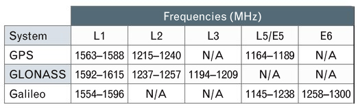
    As the bandwidth requirement of an antenna increases, the antenna becomes harder to design, and developing an antenna that covers all of these bands and making it compliant with all of the other requirements is a challenge.

    If small size is also a requirement, some level of compromise will be needed.

    Gain Pattern. For a transmitting antenna, gain is the ratio of the radiation intensity in a given direction to the radiation that would be obtained if the power accepted by the antenna was radiated isotropically. For a receiving antenna, it is the ratio of the power delivered by the antenna in response to a signal arriving from a given direction compared to that delivered by a hypothetical isotropic reference antenna. The spatial variation of an antenna’s gain is referred to as the radiation pattern or the receiving pattern. Actually, under the antenna reciprocity theorem, these patterns are identical for a given antenna and, ignoring losses, can simply be referred to as the gain pattern.

    The receiver operates best with only a small difference in power between the signals from the various satellites being tracked and ideally the antenna covers the entire hemisphere above it with no variation in gain. This has to do with potential cross-correlation problems in the receiver and the simple fact that excessive gain roll-off may cause signals from satellites at low elevation angles to drop below the noise floor of the receiver.

    On the other hand, optimization for multipath rejection and antenna noise temperature (see below) require some gain roll-off.

    FIGURE 1. Theoretical antenna with hemispherical gain pattern. Boresight corresponds to θ = 0°.
    FIGURE 1. Theoretical antenna with hemispherical gain pattern. Boresight corresponds to θ = 0°. (Data: Gerald J. K. Moernaut and Daniel Orban)

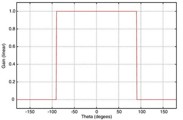
    FIGURE 1 shows what a perfect hemispherical gain pattern looks like, with a cut through an arbitrary azimuth.

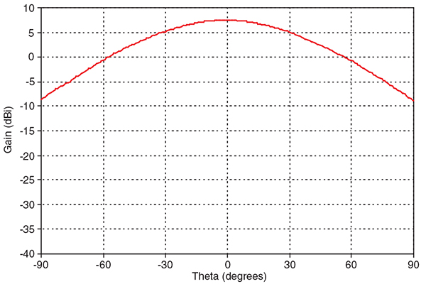
    However, such an antenna cannot be built and “real-world” GNSS antennas see a gain roll-off of 10 to 20 dB from boresight (looking straight up from the antenna) to the horizon. FIGURE 2 shows what a typical gain pattern looks like as a cross-section through an arbitrary azimuth.

    FIGURE 2. "Real-world" antenna gain pattern.
    FIGURE 2. “Real-world” antenna gain pattern. (Data: Gerald J. K. Moernaut and Daniel Orban)

    Circular Polarization. Spaceborne systems at L-Band typically use circular polarization (CP) signals for transmitting and receiving. The changing relative orientation of the transmitting and receiving CP antennas as the satellites orbit the Earth does not cause polarization fading as it does with linearly polarized signals and antennas. Furthermore, circular polarization does not suffer from the effects of Faraday rotation caused by the ionosphere. Faraday rotation results in an electromagnetic wave from space arriving at the Earth’s surface with a different polarization angle than it would have if the ionosphere was absent. This leads to signal fading and potentially poor reception of linearly polarized signals.

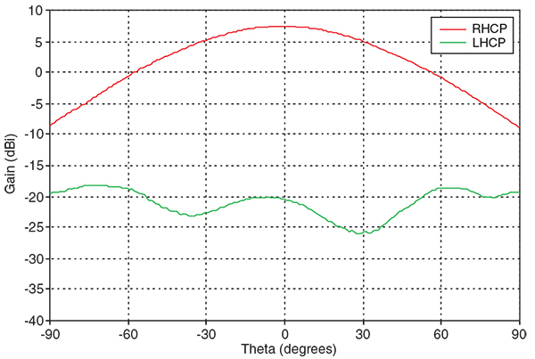
    Circularly polarized signals may either be right-handed or left-handed. GNSS satellites use right-hand circular polarization (RHCP) and therefore a GNSS antenna receiving the direct signals must also be designed for RHCP.

    Antennas are not perfect and an RHCP antenna will pick up some left-hand circular polarization (LHCP) energy. Because GPS and other GNSS use RHCP, we refer to the LHCP part as the cross-polar component (see FIGURE 3).

    FIGURE 3. Co- and cross-polar gain pattern versus boresight angle of a rover antenna.
    FIGURE 3. Co- and cross-polar gain pattern versus boresight angle of a rover antenna. (Data: Gerald J. K. Moernaut and Daniel Orban)

    We can describe the quality of the circular polarization by either specifying the ratio of this cross-polar component with respect to the co-polar component (RHCP to LHCP), or by specifying the axial ratio (AR). AR is the measure of the polarization ellipticity of an antenna designed to receive circularly polarized signals. An AR close to 1 (or 0 dB) is best (indicating a good circular polarization) and the relationship between the co-/cross-polar ratio and axial ratio is shown in FIGURE 4.

    FIGURE 4. Converting axial ratio to co-/cross-polar ratio.
    FIGURE 4. Converting axial ratio to co-/cross-polar ratio. (Data: Gerald J. K. Moernaut and Daniel Orban)
    FIGURE 5. Co-/cross-polar and axial ratios versus boresight angle of a rover-style antenna.
    FIGURE 5. Co-/cross-polar and axial ratios versus boresight angle of a rover-style antenna. (Data: Gerald J. K. Moernaut and Daniel Orban)

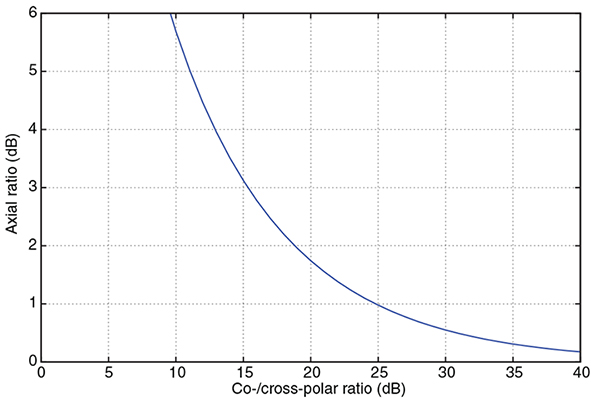
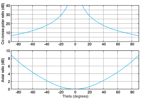
    FIGURE 5 shows the ratio of the co- and cross-polar components and the axial ratio versus boresight (or depression) angle for a typical GPS antenna. The boresight angle is the complement of the elevation angle.

    For high-end GNSS antennas such as choke-ring and other geodetic-quality antennas, the typical AR along the boresight should be not greater than about 1 dB. AR increases towards lower elevation angles and you should look for an AR of less than 3 to 6 dB at a 10° elevation angle for a high-performance antenna. Expect to see small (<1 dB) variations of AR versus azimuth at the low elevation angles.

    Maintaining a good AR over the entire hemisphere and at all frequencies requires a lot of surface area in the antenna and can only be accomplished in high-end antennas like base station and rover antennas.

    Multipath Suppression. Signals coming from the satellites arrive at the GNSS receiver’s antenna directly from space, but they may also be reflected off the ground, buildings, or other obstacles and arrive at the antenna multiple times and delayed in time. This is termed multipath. It degrades positioning accuracy and should be avoided. High-end receivers are able to suppress multipath to a certain extent, but it is good engineering practice to suppress multipath in the antenna as much as possible.

    A multipath signal can come from three basic directions:

    • The ground and arrive at the back of the antenna.
    • The ground or an object and arrive at the antenna at a low elevation angle.
    • An object and arrive at the antenna at a high elevation angle.

    Reflected signals typically contain a large LHCP component. The technique to mitigate each of these is different and, as an example, we will describe suppression of multipath signals due to ground and vertical object reflections.

    Multipath susceptibility of an antenna can be quantified with respect to the antenna’s gain pattern characteristics by the multipath ratio (MPR). FIGURE 6 sketches the multipath problem due to ground reflections.

    FIGURE 6. Quantifying multipath caused by ground reflections.
    FIGURE 6. Quantifying multipath caused by ground reflections. (Data: Gerald J. K. Moernaut and Daniel Orban)

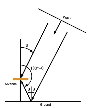
    We can derive this MPR formula for ground reflections:

    Data: Gerald J. K. Moernaut and Daniel Orban

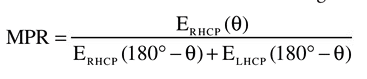
    The MPR for signals that are reflected from the ground equals the RHCP antenna gain at a boresight angle (θ) divided by the sum of the RHCP and LHCP antenna gains at the supplement of that angle.

    Signals that are reflected from the ground require the antenna to have a good front-to-back ratio if we want to suppress them because an RHCP antenna has by nature an LHCP response in the anti-boresight or backside hemisphere. The front-to-back ratio is nominally the difference in the boresight gain and the gain in the anti-boresight direction. A good front-to-back ratio also minimizes ground-noise pick-up.

    Similarly, an MPR formula can be written for signals that reflect against vertical objects. FIGURE 7 sketches this.

    FIGURE 7. Quantifying multipath caused by vertical object reflections.
    FIGURE 7. Quantifying multipath caused by vertical object reflections. (Data: Gerald J. K. Moernaut and Daniel Orban)

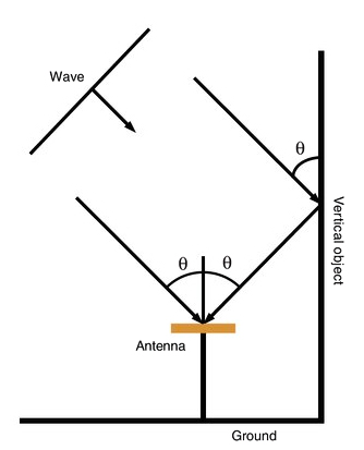
    And the formula looks like this:

    Data: Gerald J. K. Moernaut and Daniel Orban

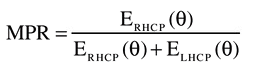
    The MPR for signals that are reflected from vertical objects equals the RHCP antenna gain at a boresight angle (θ) divided by the sum of the RHCP and LHCP antenna gains at that angle.

    Multipath signals from reflections against vertical objects such as buildings can be suppressed by having a good AR at those elevation angles from which most vertical object multipath signals arrive. This AR requirement is readily visible in the MPR formula considering these reflections are predominantly LHCP, and in this case MPR simply equals the co- to cross-polar ratio.

    LHCP reflections that arrive at the antenna at high elevation angles are not a problem because the AR tends to be quite good at these elevation angles and the reflection will be suppressed. LHCP signals arriving at lower elevation angles may pose a problem because the AR of an antenna at low elevation angles is degraded in “real-world” antennas. It makes sense to have some level of gain roll-off towards the lower elevation angles to help suppress multipath signals. However, a good AR is always a must because gain roll-off alone will not do not it.

    Phase Center. A position fix in GNSS navigation is relative to the electrical phase center of the antenna. The phase center is the point in space where all the rays appear to emanate from (or converge on) the antenna. Put another way, it is the point where the electromagnetic fields from all incident rays appear to add up in phase. Determining the phase center is important in GNSS applications, particularly when millimeter-positioning resolution is desired.

    Ideally, this phase center is a single point in space for all directions at all frequencies. However, a “real-world” antenna will often possess multiple phase center points (for each lobe in the gain pattern, for example) or a phase center that appears “smeared out” as frequency and viewing angle are varied.

    The phase-center offset can be represented in three dimensions where the offset is specified for every direction at each frequency band. Alternatively, we can simplify things and average the phase center over all azimuth angles for a given elevation angle and define it over the 10° to 90° elevation-angle range. For most applications even this simplified representation is over-kill, and typically only a vertical and a horizontal phase-center offset are specified for all bands in relation to L1.

    For well-designed high-end GNSS antennas, phase center variations in azimuth are small and on the order of a couple of millimeters. The vertical phase offsets are typically 10 millimeters or less. Many high-end antennas have been calibrated, and tables of phase-center offsets for these antennas are available.

    Impact on Receiver Sensitivity. The strength of the signals from space is on the order of -130 dBm. We need a really sensitive receiver if we want to be able to pick these up. For the antenna, this translates into the need for a high-performance low noise amplifier (LNA) between the antenna element itself and the receiver.

    We can characterize the performance of a particular receiver element by its noise figure (NF), which is the ratio of actual output noise of the element to that which would remain if the element itself did not introduce noise. The total (cascaded) noise figure of a receiver system (a chain of elements or stages) can be calculated using the Friss formula as follows:

    Data: Gerald J. K. Moernaut and Daniel Orban

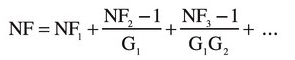
    The total system NF equals the sum of the NF of the first stage (NF1) plus that of the second stage (NF2) minus 1 divided by the total gain of the previous stage (G1) and so on. So the total NF of the whole system pretty much equals that of the first stage plus any losses ahead of it such as those due to filters.

    Expect to see total LNA noise figures in the 3-dB range for high performance GNSS antennas.

    The other requirement for the LNA is for it to have sufficient gain to minimize the impact of long and lossy coaxial antenna cables — typically 30 dB should be enough. Keep in mind that it is important to have the right amount of gain for a particular installation. Too much gain may overload the receiver and drive it into non-linear behavior (compression), degrading its performance. Too little, and low-elevation-angle observations will be missed. Receiver manufacturers typically specify the required LNA gain for a given cable run.

    Interference Handling. Even though GNSS receivers are good at mitigating some kinds of interference, it is essential to keep unwanted signals out of the receiver as much as possible. Careful design of the antenna can help here, especially by introducing some frequency selectivity against out-of-band interferers. The mechanisms by which in-band an out-of-band interference can create trouble in the LNA and the receiver and the approach to dealing with them are somewhat different.

    FIGURE 8. Strong out-of-band interferer and third harmonic in the GPS L1 band.
    FIGURE 8. Strong out-of-band interferer and third harmonic in the GPS L1 band. (Data: Gerald J. K. Moernaut and Daniel Orban)

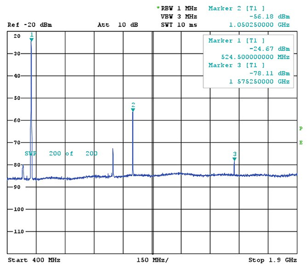
    An out-of-band interferer is generally an RF source outside the GNSS frequency bands: cellular base stations, cell phones, broadcast transmitters, radar, etc. When these signals enter the LNA, they can drive the amplifier into its non-linear range and the LNA starts to operate as a multiplier or comb generator. This is shown in FIGURE 8 where a -30-dBm-strong interferer at 525 MHz generates a -78 dBm spurious signal or spur in the GPS L1 band.

    Through a similar mechanism, third-order mixing products can be generated whereby a signal is multiplied by two and mixes with another signal. As an example, take an airport where radars are operating at 1275 and 1305 MHz. Both signals double to 2550 and 2610 MHz. These will in turn mix with the fundamentals and generate 1245 and 1335 MHz signals.

    Another mechanism is de-sensing: as the interference is amplified further down in the LNA’s stages, its amplitude increases, and at some point the GNSS signals get attenuated because the LNA goes into compression. The same thing may happen down the receiver chain. This effectively reduces the receiver’s sensitivity and, in some cases, reception will be lost completely.

    RF filters can reduce out-of-band signals by 10s of decibels and this is sufficient in most cases. Of course, filters add insertion loss and amplitude and phase ripple, all of which we don’t want because these degrade receiver performance.

    In-band interferers can be the third-order mixing products we mentioned above or simply an RF source that transmits inside the GNSS bands. If these interferers are relatively weak, the receiver will handle them, but from a certain power level on, there is just not a lot we can do in a conventional commercial receiver.

    The LNA should be designed for a high intercept point (IP)–at which non-linear behavior begins–so compression does not occur with strong signals present at its input. On the other hand, there is no requirement for the LNA to be a power amplifier. As an example, let’s say we have a single strong continuous wave interferer in the L1 band that generates -50 dBm at the input of the LNA. A 50 dB, high IP LNA will generate a 0 dBm carrier in the L1 band but the receiver will saturate.

    LNAs with a higher IP tend to consume more power and in a portable application with a rover antenna — that may be an issue. In a base-station antenna, on the other hand, low current consumption should not be a requirement since a higher IP is probably more valuable than low power consumption.

    GNSS Antenna Types

    Here is a short comparison of three types of GNSS antennas: geodetic, rover, and handheld. For detailed specifications of examples of each of these types, see the references in Further Reading.

    Geodetic Antennas. High precision, fixed-site GNSS applications require geodetic-class receivers and antennas. These provide the user with the highest possible position accuracy.

    As a minimum, typical geodetic antennas cover the GPS L1 and L2 bands. Some also cover the GLONASS frequencies. Coverage of L5 is found in some newer designs as well as coverage of the Galileo frequencies and the L-band frequencies of differential GNSS services.

    The use of choke-ring ground planes is typical in geodetic antennas. These allow good gain pattern control, excellent multipath suppression, high front-to-back ratio, and good AR at low elevation angles. Choke rings contribute to a stable phase center. The phase center is documented (as mentioned earlier), and high-end receivers allow the antenna behavior to be taken into account. Combined with a state-of-the-art LNA, these antennas provide the highest possible performance.

    Rover Antennas. Rover antennas are typically used in land survey, forestry, construction, and other portable or mobile applications. They provide the user with good accuracy while being optimized for portability.  Horizontal phase-center variation versus azimuth should be low because the orientation of the antenna with respect to magnetic north, say, is usually unknown and cannot be corrected for in the receiver.  A rover antenna is typically mounted on a handheld pole. Good front-to-back ratio is required to avoid operator-reflection multipath and ground-noise pickup.  Yet these rover-type applications are high accuracy and require a good phase-center stability. However, since a choke ring cannot be used because of its size and weight, a higher phase-center variation compared to that of a geodetic antenna is typically inherent to the rover antenna design.

    A good AR and a decent gain roll-off at low elevation angles ensures good multipath suppression as heavy choke rings are not an option for this configuration.

    Handheld Receiver Antennas. These antennas are single-band L1 structures optimized for size and cost. They are available in a range of implementations, such as surface mount ceramic chip, helical, and patch antenna types. Their radiation patterns are quasi-hemispherical. AR and phase-center performance are a compromise because of their small size. Because of their reduced size, these antennas tend to have a negative gain of about -3 dBi (3 dB less than an ideal isotropic antenna) at boresight. This negative gain is mostly masked by an embedded LNA. The associated elevated noise figure is typically not an issue in handheld applications.

    TABLE 2. Characteristics of different GNSS antenna classes.
    TABLE 2. Characteristics of different GNSS antenna classes. (Data: Gerald J. K. Moernaut and Daniel Orban)

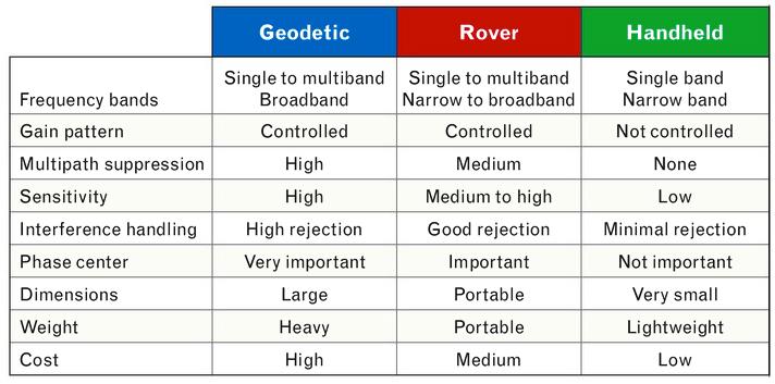
    Summary of Antenna Types. TABLE 2 presents a comparison of the most important properties of geodetic, rover, and handheld types of GNSS antennas.

    Conclusion

    In this article, we have presented an overview of the most important characteristics of GNSS antennas. Several GNSS receiver-antenna classes were discussed based on their typical characteristics, and the resulting specification compromises were outlined. Hopefully, this information will help you select the right antenna for your next GNSS application.

    Acknowledgment

    An earlier version of this article entitled “Basics of GPS Antennas” appeared in The RF & Microwave Solutions Update, an online publication of RF Globalnet.


    GERALD J. K. MOERNAUT holds an M.Sc. degree in electrical engineering. He is a full-time antenna design engineer with Orban Microwave Products, a company that designs and produces RF and microwave subsystems and antennas with offices in Leuven, Belgium, and El Paso, Texas.

    DANIEL ORBAN is president and founder of Orban Microwave Products. In addition to managing the company, he has been designing antennas for a number of years.


    FURTHER READING

    Previous GPS World Articles on GNSS Antennas

    “Getting into Pockets and Purses: Antenna Counters Sensitivity Loss in Consumer Devices” by B. Hurte and O. Leisten in GPS World, Vol. 16, No. 11, November 2005, pp. 34-38.

    “Characterizing the Behavior of Geodetic GPS Antennas” by B.R. Schupler and T.A. Clark in GPS World, Vol. 12, No. 2, February 2001, pp. 48-55.

    “A Primer on GPS Antennas” by R.B. Langley in GPS World, Vol. 9, No. 7, July 1998, pp. 50-54.

    “How Different Antennas Affect the GPS Observable” by B.R. Schupler and T.A. Clark in GPS World, Vol. 2, No. 10, November 1991, pp. 32-36.

    Introduction to Antennas and Receiver Noise

    “GNSS Antennas and Front Ends” in A Software-Defined GPS and Galileo Receiver: A Single-Frequency Approach by K. Borre, D.M.Akos, N. Bertelsen, P. Rinder, and S.H. Jensen, Birkhäuser Boston, Cambridge, Massachusetts, 2007.

    The Technician’s Radio Receiver Handbook: Wireless and Telecommunication Technology by J.J. Carr, Newnes Press, Woburn, Massachusetts, 2000.

    “GPS Receiver System Noise” by R.B. Langley in GPS World, Vol. 8, No. 6, June 1997, pp. 40-45.

    More on GNSS Antenna Types

    “The Basics of Patch Antennas” by D. Orban and G.J.K. Moernaut. Available on the Orban Microwave Products website.

    Project Examples

    Interference in GNSS Receivers

    “Interference Heads-Up: Receiver Techniques for Detecting and Characterizing RFI” by P.W. Ward in GPS World, Vol. 19, No. 6, June 2008, pp. 64-73.

    “Jamming GPS: Susceptibility of Some Civil GPS Receivers” by B. Forssell and T.B. Olsen in GPS World, Vol. 14, No. 1, January 2003, pp. 54-58.

  • GAARDIAN Consortium Wins GPS/eLoran Integrity Research Project

    A business and academic consortium led by Chronos Technology has received a major grant from the U.K. government sponsored Technology Strategy Board for a £2.2 million (approximately $3.3 million) research project to improve the safety and security of location-based applications such as marine navigation and road transportation.

    The consortium has dubbed the project GAARDIAN, or GNSS Availability, Accuracy, Reliability and Integrity Assessment for Timing and Navigation. Over the next 30 months, the consortium will be developing a system for mission and safety critical applications that will certify the accuracy, reliability, and integrity of positioning, navigation and timing systems, namely GPS, enhanced Loran (eLoran), and GLONASS.

    “GPS is fast becoming an unseen, embedded and low cost commodity. The challenge to the user community is that it may not appreciate the fact that subtle failures of the GPS signal could have disastrous or expensive consequences in mission or safety critical applications,” said Charles Curry, managing director of Chronos Technology. “The impact on GPS from threats such as jamming, spoofing, space-weather, multipath and other types of interference is likely to increase over the coming years due for example to easier availability of jamming technology or more esoteric phenomena such as increased sun-spot activity. The GAARDIAN project aims to create a data gathering system that will enable any user to monitor the health of the GPS signal in the vicinity of use on a 24-7 basis in real time.”

    GAARDIAN will use the Universal Time Coordinate-traceable timing signal from the GLAs’ eLoran station at Anthorn in Cumbria, United Kingdom, along with analysis of the GPS signal data to authenticate GPS reception wherever it is needed for mission and safety critical applications. The challenge is to gather and filter large volumes of GPS and eLoran data continuously in multiple, complex and disparate environments without losing content, according to Chronos.

    “This is an exciting project that will exploit the complementary benefits of satellite and terrestrial systems to reduce risk and so improve safety and security at sea and protection of the marine environment,” said Sally Basker, director of research and radionavigation for the General Lighthouse Authorities.

    The consortium brings together seven private, public, and academic organizations: Chronos Technology, BT Design, the General Lighthouse Authorities of the United Kingdom and Ireland, the Imperial College London, the (U.K.) National Physical Laboratory, the Ordnance Survey of Great Britain, and the University of Bath

  • Innovation: Tsunami Detection by GPS

    Innovation: Tsunami Detection by GPS

    QuickBird satellite image of Kalutara Beach on the southwestern coast of Sri Lanka showing the receding waters and beach damage from the Sumatra tsunami.
    QuickBird satellite image of Kalutara Beach on the southwestern coast of Sri Lanka showing the receding waters and beach damage from the Sumatra tsunami.( Credit: Digital Globe)

    How Ionospheric Observations Might Improve the Global Warning System

    By Giovanni Occhipinti, Attila Komjathy, and Philippe Lognonné

    Recent investigations have demonstrated that GPS might be an effective tool for improving the tsumani early-warning system through rapid determination of earthquake magnitude using data from GPS networks. A less obvious approach is to use the GPS data to look for the tsunami signature in the ionosphere.

    INNOVATION INSIGHTS by Richard Langley
    INNOVATION INSIGHTS by Richard Langley

    THE TSUNAMI generated by the December 26, 2004, earthquake just off the coast of the Indonesian island of Sumatra killed over 200,000 people. It was one of the worst natural disasters in recorded history. But it might have been largely averted if an adequate warning system had been in place.

    A tsunami is generated when a large oceanic earthquake causes a rapid displacement of the ocean floor. The resulting ocean oscillations or waves, while only on the order of a few centimeters to tens of centimeters in the open ocean, can grow to be many meters even tens of meters when they reach shallow coastal areas. The speed of propagation of tsunami waves is slow enough, at about 600 to 700 kilometers per hour, that if they can be detected in the open ocean, there would be enough time to warn coastal communities of the approaching waves, giving people time to flee to higher ground.

    Seismic instruments and models are used to predict a possible tsunami following an earthquake and ocean buoys and pressure sensors on the ocean bottom are used to detect the passage of tsunami waves. But globally, the density of such instrumentation is quite low and, coupled with the time lag needed to process the data to confirm a tsunami, an effective global tsunami warning system is not yet in place.

    However, recent investigations have demonstrated that GPS might be a very effective tool for improving the warning system. This can be done, for example, through rapid determination of earthquake magnitude using data from existing GPS networks. And, incredible as it might seem, another approach is to use the GPS data to look for the tsunami signature in the ionosphere: the small displacement of the ocean surface displaces the atmosphere and makes it all the way to the ionosphere, causing measurable changes in ionospheric electron density.

    In this month’s column, we look in detail at how a tsunami can affect the ionosphere and how GPS measurements of the effect might be used to improve the global tsunami warning system.


    “Innovation” is a regular column that features discussions about recent advances in GPS technology and its applications as well as the fundamentals of GPS positioning. The column is coordinated by Richard Langley of the Department of Geodesy and Geomatics Engineering at the University of New Brunswick.


    The December 26, 2004, earthquake-generated Sumatra tsunami caused enormous losses in life and property, even in locations relatively far away from the epicentral area. The losses would likely have never been so massive had an effective worldwide tsunami warning system been in place. A tsunami travels relatively slowly and it takes several hours for one to cross the Indian Ocean, for example. So a warning system should be able to detect a tsunami and provide an alert to coastal areas in its path. Among the strengths of a tsunami early-warning system would be its capability to provide an estimate of the magnitude and location of an earthquake. It should also confirm the amplitude of any associated tsunami, due to massive displacement of the ocean bottom, before it reaches populated areas. In the aftermath of the Sumatra tsunami, an important effort is underway to interconnect seismic networks and to provide early alarms quantifying the level of tsunami risk within 15 minutes of an earthquake.

    However, the seismic estimation process cannot quantify the exact amplitude of a tsunami, and so the second step, that of tsunami confirmation, is still a challenge. The earthquake fault mechanism at the epicenter cannot fully explain the initiation of a tsunami as it is only approximated by the estimated seismic source. The fault slip is not transmitted linearly at the ocean bottom due to various factors including the effect of the bathymetry, the fault depth, and the local lithospheric properties as well as possible submarine landslides associated with the earthquake.

    In the open ocean, detecting, characterizing, and imaging tsunami waves is still a challenge. The offshore vertical tsunami displacement (on the order of a few centimeters up to half a meter in the case of the Sumatra tsunami) is hidden in the natural ocean wave fluctuations, which can be several meters or more. In addition, the number of offshore instruments capable of tsunami measurements, such as tide gauges and buoys, is very limited. For example, there are only about 70 buoys in the whole world. As a tsunami propagates with a typical speed of 600–700 kilometers per hour, a 15-minute confirmation system would require a worldwide buoy network with a 150-kilometer spacing.

    Satellite altimetry has recently proved capable of measuring the sea surface variation in the case of large tsunamis, including the December 2004 Sumatra event. However, satellites only supply a few snapshots along the sub-satellite tracks. Optical imaging of the shore hs successfully measured the wave arrival at the coastline (see ABOVE PHOTO), but it is ineffective in the open sea. At present, only ocean-bottom sensors and GPS buoy receivers supply measures of mid-ocean vertical displacement. In many cases, the tsunami can only be identified several hours after the seismic event due to the poor distribution of sensors. This delay is necessary for the tsunami to reach the buoys and for the signal to be recorded for a minimum of one wave period (a typical tsunami wave period is between 10 and 40 minutes) to be adequately filtered by removing the “noise” due to normal wave action.

    In the case of the December 2004 Sumatra event, the first tsunami measurements by any instrumentation were only made available about 3 hours after the earthquake. They were supplied by the real-time tide gauge at the Cocos Islands, an Australian territory in the southeast Indian Ocean (see FIGURE 1 where the tsunami signature is superimposed on the large semidiurnal tide fluctuation). Up until that time, the tsunami could not be fully confirmed and coastal areas remained vulnerable to tsunami damage. This delay in confirmation is a fundamental weakness of the existing tsunami warning systems.

    Figure 1. The Sumatra tsunami signal measured at the Cocos Islands by the tide gauge (red) and by the co-located GPS receiver (blue). The tide gauge measures the sea-level displacement (tide plus superimposed tsunami) and the GPS receiver measures the slant total electron content perturbation (+/-1 TEC unit) in the ionosphere.
    Figure 1. The Sumatra tsunami signal measured at the Cocos Islands by the tide gauge (red) and by the co-located GPS receiver (blue). The tide gauge measures the sea-level displacement (tide plus superimposed tsunami) and the GPS receiver measures the slant total electron content perturbation (+/-1 TEC unit) in the ionosphere.

    Ionospheric Perturbation. Recently, observational and modeling results have confirmed the existence and detectability of a tsunamigenic signature in the ionosphere. Physically, the displacement induced by tsunamis at the sea surface is transmitted into the atmosphere where it produces internal gravity waves (IGWs) propagating upward. (When a fluid or gas parcel is displaced at an interface, or internally, to a region with a different density, gravity restores the parcel toward equilibrium resulting in an oscillation about the equilibrium state; hence the term gravity wave.) The normal ocean surface variability has a typical high frequency (compared to tsunami waves) and does not transfer detectable energy into the atmosphere. In other words, the Earth’s atmosphere behaves as an “analog low-pass filter.” Only a tsunami produces propagating waves in the atmosphere. During the upward propagation, these waves are strongly amplified by the double effects of the conservation of kinetic energy and the decrease of atmospheric density resulting in a local displacement of several tens of meters per second at 300 kilometers altitude in the atmosphere. This displacement can reach a few hundred meters per second for the largest events.

    At an altitude of about 300 kilometers, the neutral atmosphere is strongly coupled with the ionospheric plasma producing perturbations in the electron density. These perturbations are visible in GPS and satellite altimeter data since those signals have to transit the ionosphere. The dual-frequency signal emitted by GPS satellites can be processed to obtain the integral of electron density along the paths between the satellites and the receiver, the total electron content (TEC).

    Within about 15 minutes, the waves generated at the sea surface reach ionospheric altitudes, creating measurable fluctuations in the ionospheric plasma and consequently in the TEC. This indirect method of tsunami detection should be helpful in ocean monitoring, allowing us to follow an oceanic wave from its generation to its propagation in the open ocean.

    So, can ionospheric sounding provide a robust method of tsunami confirmation? It is our hope that in the future this technique can be incorporated into a tsunami early-warning system and complement the more traditional methods of detection including tide gauges and ocean buoys. Our research focuses on whether ground-based GPS TEC measurements combined with a numerical model of the tsunami-ionosphere coupling could be used to detect tsunamis robustly. Such a detection scheme depends on how the ionospheric signature is related to the amplitude of the sea surface displacement resulting from a tsunami. In the near future, the ionospheric monitoring of TEC perturbations might become an integral part of a tsunami warning system that could potentially make it much more effective due to the significantly increased area of coverage and timeliness of confirmation.

    In this article, we’ll take a look at the current state of the art in modeling tsunami-generated ionospheric perturbations and the status of attempts to monitor those perturbations using GPS.

    Some Background

    Pioneering work by the Canadian atmospheric physicist Colin Hines in the 1970s suggested that tsunami-related IGWs in the atmosphere over the oceanic regions, while interacting with the ionospheric plasma, might produce signatures detectable by radio sounding.

    In June 2001, an episodic perturbation was observed following a tsunamigenic earthquake in Peru. After its propagation across the Pacific Ocean (taking about 22 hours), the tsunami reached the Japanese coast and its signature in the ionosphere was detected by the Japanese GPS dense network (GEONET). The perturbation, shown in FIGURE 2, has an arrival time and characteristic period consistent with the tsunami propagation determined from independent methods. Unfortunately, similar signatures in the ionosphere are also produced by IGWs associated with traveling ionospheric disturbances (TIDs), and are commonly observed in the TEC data. However, the known azimuth, arrival time, and structure of the tsunami allows us to use this data source, even if it contains background TIDs.

    Figure 2. The observed signal for the June 23, 2001, tsunami (initiated offshore Peru). Total electron content variations are plotted at the ionosphere pierce points. A wave-like disturbance is seen propagating toward the coast of Honshu, the main island of Japan.
    Figure 2. The observed signal for the June 23, 2001, tsunami (initiated offshore Peru). Total electron content variations are plotted at the ionosphere pierce points. A wave-like disturbance is seen propagating toward the coast of Honshu, the main island of Japan.

    The December 26, 2004, Sumatra earthquake, with a magnitude of 9.3, was an order of magnitude larger than the Peru event and was the first earthquake and tsunami of magnitude larger than 9 of the so-called “human digital era,” comparable to the magnitude 9.5 Chilean earthquake of May 22, 1960.

    In addition to seismic waves registered by global seismic networks, the Sumatra event produced infragravity waves (long-period wave motions with typical periods of 50 to 200 seconds) remotely observed from the island of Diego Garcia, perturbations in the magnetic field observed by the CHAMP satellite, and a series of ionospheric anomalies.

    Two types of ionospheric anomaly were observed: anomalies of the first type, detected worldwide in the first few hours after the earthquake, were reported from north of Sumatra, in Europe, and in Japan. They are associated with the surface seismic waves that propagate around the world after an earthquake rupture (so-called Rayleigh waves).

    Anomalies of the second type were detected above the ocean and were clearly associated with the tsunami. In the Indian Ocean, the occurrence times of TEC perturbations observed using ground-based GPS receivers and satellite altimeters were consistent with the observed tsunami propagation speed. The GPS observations from sites to the north of Sumatra show internal gravity waves most likely coupled with the tsunami or generated at the source and propagating independently in the atmosphere. The link with the tsunami is more evident in the observations elsewhere in the Indian Ocean. The TEC perturbations observed by the other ground-based GPS receivers moved horizontally with a velocity coherent with the tsunami propagation.

    Figure 3. The tsunamigenic earthquake mechanism and transfer of energy in the neutral and ionized atmosphere. The solid Earth displacement produces the tsunami and the sea surface displacement produces an internal gravity wave in the neutral atmosphere, which perturbs the electron distribution in the ionosphere.
    Figure 3. The tsunamigenic earthquake mechanism and transfer of energy in the neutral and ionized atmosphere. The solid Earth displacement produces the tsunami and the sea surface displacement produces an internal gravity wave in the neutral atmosphere, which perturbs the electron distribution in the ionosphere.

    The amplitude of the observed TEC perturbations is strongly dependent on the filter method used. The four TECU-level peak-to-peak variations in filtered GPS TEC measurements from north of Sumatra are coherent with the differential TEC at the 0.4 TECU per 30 seconds level observed in the rest of the Indian Ocean. (One TEC unit or TECU is 1016 electrons per meter-squared, equivalent to 0.162 meters of range delay at the GPS L1 frequency.) Such magnitudes can be detected using GPS measurements since GPS phase observables are sensitive to TEC fluctuations at the 0.01 TECU level. We emphasize also the role of the elevation angle in the detection of tsunamigenic perturbations in the ionosphere. As a consequence of the integrated nature of TEC and the vertical structure of the tsunamigenic perturbation, low-elevation angle geometry is more sensitive to the tsunami signature in the GPS data, hence it is more visible.

    The TEC perturbation observed at the Cocos Islands by GPS can be compared with the co-located tide-gauge (Figure 1). The tsunami signature in the data from the two different instruments shows a similar waveform, confirming the sensitivity of the ionospheric measurement to the tsunami structure.

    The link between the tsunami at sea level and the perturbation observed in the ionosphere has been demonstrated using a 3D numerical modeling based on the coupling between the ocean surface, the neutral atmosphere, and the ionosphere (see FIGURE 3). The modeling reproduced the TEC data with good agreement in amplitude as well as in the waveform shape, and quantified it by a cross-correlation (see FIGURE 4). The resulting shift of +/-1 degree showed the presence of zonal and meridional winds neglected in the modeling. The presence of the wind can, indeed, introduce a shift of 1 degree in latitude and 1.5 degrees in longitude.

    Since modeling is an effective method to discriminate between the tsunami signature in the ionosphere and other potential perturbations, the GPS observations can be a useful tool to develop an inexpensive tsunami detection system based on the ionospheric sounding.

    Figure 4. Satellite altimeter and total electron content (TEC) signatures of the Sumatra tsunami. The modeled and observed TEC is shown for (a) Jason-1 and for (b) Topex/Poseidon: data (black), synthetic TEC without production-recombination-diffusion effects (blue), with production-recombination (red), and production-recombination-diffusion (green). The Topex/Poseidon synthetic TEC has been shifted up by 2 TEC units. In (c) and (d), the altimetric measurements of the ocean surface (black) are plotted for the Jason-1 and Topex/Poseidon satellites, respectively. The synthetic ocean displacement, used as the source of internal gravity waves in the neutral atmosphere, is shown in red. In (e), the cross-correlations between TEC synthetics and data are shown for Jason-1 (blue) and Topex/Poseidon (red).
    Figure 4. Satellite altimeter and total electron content (TEC) signatures of the Sumatra tsunami. The modeled and observed TEC is shown for (a) Jason-1 and for (b) Topex/Poseidon: data (black), synthetic TEC without production-recombination-diffusion effects (blue), with production-recombination (red), and production-recombination-diffusion (green). The Topex/Poseidon synthetic TEC has been shifted up by 2 TEC units. In (c) and (d), the altimetric measurements of the ocean surface (black) are plotted for the Jason-1 and Topex/Poseidon satellites, respectively. The synthetic ocean displacement, used as the source of internal gravity waves in the neutral atmosphere, is shown in red. In (e), the cross-correlations between TEC synthetics and data are shown for Jason-1 (blue) and Topex/Poseidon (red).

    Modeling TEC Perturbations

    A model to describe the effect of a tsunami on the ionosphere has been developed at the Institut de Physique du Globe de Paris (IPGP), France. It is comprised of three main parts. Firstly, it computes tsunami propagation using realistic bathymetry of, for example, the Indian Ocean. Secondly, an oceanic displacement is used to excite IGWs in the neutral atmosphere. Thirdly, it computes the response of the ionosphere induced by the neutral atmospheric motion resulting in enhanced electron densities. After integrating the electron densities, we obtain modeled (synthetic) TEC data. The modeling steps are as follows:

    Tsunami Propagation. Tsunami modeling is an established science and the propagation of tsunamis is generally based on a shallow-water hypothesis. Under this hypothesis, the ocean is considered as a simple layer where the ocean depth, h, is locally taken into account in the tsunami propagation velocity, v = √ hg, which directly depends on h and the gravity acceleration g. The modeling, usually based on finite differences, solves the appropriate hydrodynamic equations.

    Neutral Atmosphere Coupling. A tsunami is an oceanic gravity wave and its propagation is not limited to the oceanic surface; as previously discussed, the ocean displacement is transferred to the atmosphere where it becomes an internal gravity wave. This coupling phenomenon is linear and can be reproduced solving the wave propagation equations, nominally the continuity and the so-called Navier-Stokes equations. These equations are solved assuming the atmosphere to be irrotational, inviscid, and incompressible. The IGWs are, indeed, imposed by displacement of the mass under the effect of the gravity force, contrary to the elastic waves generated by compression (for example, sound waves), so the medium can be considered incompressible. FIGURE 5 shows the IGWs produced by the Sumatra tsunami. The inversion of the velocity with altitude (wind shear) is a typical structure of IGWs.

    Neutral-Plasma Coupling. The tsunamigenic IGWs are injected into a 3D ionospheric model to reproduce the induced electron density perturbations. In essence, the coupling model solves the hydromagnetic equations for three ion species (O2 + , NO+ , and O+ ). Physically, the neutral atmosphere motion induces fluctuations in the plasma velocity by way of momentum transfer driven by collision frequency and the Lorentz term associated with Earth’s magnetic and electric fields. Ion loss, recombination, and diffusion are also taken into account in the ion continuity equation. Finally, the perturbed electron density is inferred from ion densities using the charge neutrality hypothesis. The International Reference Ionosphere model is used for background electron density; SAMI2 (a recursive acronym: SAMI2 is Another Model of the Ionosphere) is used for collision, production, and loss parameters; and a constant geomagnetic field is assumed based on the International Geomagnetic Reference Field. FIGURE 5 shows the perturbation induced in the ionospheric plasma by the tsunamigenic IGW following the Sumatra event. The perturbation is strongly localized to around 300 kilometers altitude where the electron density background is maximized.

    Figure 5. Internal gravity waves (IGWs) generated by the Sumatra tsunami and the response of the ionosphere to neutral motion at 02:40 UT (almost two hours after the earthquake). On the left, the normalized vertical velocity induced by tsunami-generated IGWs in the neutral atmosphere is shown. On the right, the perturbation induced by IGWs in the ionospheric plasma (in electrons per cubic meter) is shown, with the maximum perturbation at an altitude of about 300 kilometers. The vertical cut shown in these profiles is at a latitude of -1 degree.
    Figure 5. Internal gravity waves (IGWs) generated by the Sumatra tsunami and the response of the ionosphere to neutral motion at 02:40 UT (almost two hours after the earthquake). On the left, the normalized vertical velocity induced by tsunami-generated IGWs in the neutral atmosphere is shown. On the right, the perturbation induced by IGWs in the ionospheric plasma (in electrons per cubic meter) is shown, with the maximum perturbation at an altitude of about 300 kilometers. The vertical cut shown in these profiles is at a latitude of -1 degree.

    The resulting electron density dynamic model described above allows us to compute a map of the perturbed TEC by simple vertical integration (see FIGURE 6). In addition to the geometrical dispersion of the tsunami, the TEC map shows horizontal heterogeneities in the electron density perturbation that are induced by the geomagnetic field inclination. The magnetic field plays a fundamental role in the neutral-plasma coupling, resulting in a strong amplification at the magnetic equator where the magnetic field is directed horizontally. The isolated perturbation appearing more to the south is probably induced by the full development of the IGW in the atmosphere. Recent work also explains this second perturbation as induced by the role of the magnetic field in the neutral-plasma coupling.

    Figure 6. The signature of the Sumatra tsunami in total electron content (TEC) at 03:18 UT (right) compared with the unperturbed TEC (left). The TEC images have been computed by vertical integration of the perturbed and unperturbed electron density fields. The broken lines represent the Topex/Poseidon (left) and Jason-1 (right) trajectories. The blue contours represent the geomagnetic field inclination.
    Figure 6. The signature of the Sumatra tsunami in total electron content (TEC) at 03:18 UT (right) compared with the unperturbed TEC (left). The TEC images have been computed by vertical integration of the perturbed and unperturbed electron density fields. The broken lines represent the Topex/Poseidon (left) and Jason-1 (right) trajectories. The blue contours represent the geomagnetic field inclination.

    GPS Data Processing

    To validate our model, we use ground-based GPS receivers to look for the ionospheric signal induced by tsunamis. Prior research has shown post-processed results detecting a tsunami-generated TEC signal using regional GPS networks such as GEONET in Japan (about 1,000 stations) or the Southern California Integrated GPS Network (about 200 stations). Those studies benefited from the very high density of GPS receivers in the regional networks, so that, for example, no forward modeling was needed to help initially identify the characteristics of the tsunami-generated signal.

    High-Precision Processing. More than 1,300 globally-distributed dual-frequency GPS receivers are available using publicly accessible networks, including those of the International GNSS Service and the Continuously Operating GPS Stations coordinated by the U.S. National Geodetic Survey. Most researchers estimate vertical ionospheric structure and, simultaneously, treat hardware-related biases as nuisance parameters. In our approach for calibrating GPS receiver and satellite inter-frequency biases, we take advantage of all available GPS receivers using a new processing technique based on the Global Ionospheric Mapping software developed at the Jet Propulsion Laboratory (JPL). FIGURE 7 shows a JPL TEC map using 1,000 GPS stations. This new capability is designed to estimate receiver biases for all stations in the global network. We solve for the instrumental biases by modeling the ionospheric delay and removing it from the observation.

    Figure 7. The total electron content (TEC) between 01:00 and 01:15 UT on December 26, 2004, at ionosphere pierce points (IPPs) provided by a global network of more than 1,000 GPS tracking stations. To highlight variations, a five-day average of TEC has been subtracted from the observed TEC.
    Figure 7. The total electron content (TEC) between 01:00 and 01:15 UT on December 26, 2004, at ionosphere pierce points (IPPs) provided by a global network of more than 1,000 GPS tracking stations. To highlight variations, a five-day average of TEC has been subtracted from the observed TEC.

    Ionospheric Warning System

    The currently implemented tsunami warning system uses seismometers to detect earthquakes and to perform an estimation of the seismic moment by monitoring seismic waves. After a potential tsunami risk is determined, ocean buoy and pressure sensors have to confirm the tsunami risk. Unfortunately, the number of available ocean buoys is limited to about 70 over the whole planet. With the existing system, it may take several hours to confirm a tsunami when taking into account both the propagation time (of tsunamis reaching buoys) and data-processing time. On the other hand, the proposed ionosphere-based tsunami detection system may only require the propagation time and data-processing delays of only up to about 15–30 minutes. GPS receivers are able to sound the ionosphere up to about 20 degrees away from the receiver location, and a dense GPS network can therefore increase the coverage of the monitored area.

    The fundamental idea behind a detection method is that we need to separate tsunami-generated TEC signatures from other sources of ionospheric disturbances. However, the tsunami-generated TEC perturbations are distinguishable because they are tied to the propagation characteristics of the tsunami. Tsunami-related fluctuations should be in the gravity-wave period domain and cohere in geometry and distance with the earthquake epicenter (for example, they show up in data on multiple satellites from multiple stations and, with increasing distance from the epicenter, at a rate related to tsunami propagation speed).

    The coupled tsunami model described earlier can also be used to compute a prediction for the tsunami-generated TEC perturbation based on the seismic displacement as an input parameter to the model. The model prediction may be used as a detection aid by indicating the location of the tsunami wave front with time. This permits us to focus our detection efforts on specific locations and times, and will allow us to discriminate signal from noise.

    The model also provides information on the expected magnitude of the TEC perturbation. This provides further value in filter discrimination. Cross-correlations can be performed on nearby observations using different satellites and stations to take advantage of tsunami-related perturbations being coherent in geometry and distance from the epicenter. Once the signal is detected in data from multiple satellites and stations, we can “track” and image the tsunami during its propagation in space and time.

    The goal of our research is to assess the feasibility of detecting tsunamis in near real time. This requires that GPS data be acquired rapidly. Rapid availability of ground-based GPS data has been demonstrated via the NASA Global Differential GPS System, a highly accurate, robust real-time GPS monitoring and augmentation system.

    Conclusions

    Earlier research using GPS-derived TEC observations has revealed TEC perturbations induced by tsunamis. However, in our research, we use a combination of a coupled ionosphere-atmosphere-tsunami model with large GPS data sets. Ground-based GPS data are used to distinguish tsunami-generated TEC perturbations from background fluctuations. Tsunamis are among the most disrupting forces humankind faces. The December 26, 2004, earthquake and resulting tsunami claimed more than 200,000 lives, with several hundreds of thousands of people injured. The damage in infrastructure and other economic losses were estimated to be in the range of tens of billions of dollars. To help prevent such a global disaster from occurring again, we suggest that ionospheric sounding by GPS be integrated into the existing tsunami warning system as soon as possible.

    Acknowledgments

    This article is based on the paper “Three-Dimensional Waveform Modeling of Ionospheric Signature Induced by the 2004 Sumatra Tsunami” published in Geophysical Research Letters. The authors wish to acknowledge François Crespon (Noveltis, Ramonville-Saint-Agne, France) for the TEC data analysis in Figure 1, Juliette Artru (Centre National d’Etudes spatiales – CNES, Toulouse, France) for her work on the detection of tsunamigenic TEC perturbations shown in this article, and Grégoire Talon for Figure 3. The IPGP portion of the work is sponsored by L’Agence Nationale de la Recherche, by CNES, and by the Ministère de l’Enseignement supérieur et de la Recherche. The first author would also like to thank John LaBrecque of NASA’s Science Mission Directorate for supporting his fellowship at the California Institute of Technology/JPL.


    GIOVANNI OCCHIPINTI received his Ph.D. at the Institut de Physique du Globe de Paris (IPGP) in 2006. In 2007, he joined NASA’s Jet Propulsion Laboratory (JPL), California Institute of Technology, as a postdoctoral fellow to continue his work on the detection and modeling of tsunamigenic perturbations in the ionosphere. He will soon take up the position of assistant professor at the University of Paris and IPGP. His scientific interests are focused on solid Earth-atmosphere-ionosphere coupling.

    ATTILA KOMJATHY is senior staff member of the Ionospheric and Atmospheric Remote Sensing Group of Tracking Systems and Applications Section at JPL, specializing in remote sensing techniques. He received his Ph.D. from the Department of Geodesy and Geomatics Engineering at the University of New Bruns-wick, Canada, in 1997. He has received the Canadian Governor General’s Gold Medal for Academic Excellence and NASA awards including an Exceptional Space Act Award.

    PHILIPPE LOGNONNÉ is the director of the Space Department of IPGP, a professor at the University of Paris VII, and a junior member of the Institut Universitaire de France. His science interests are in the field of remote sensing and are related to the detection of seismic waves and tsunamis in the ionosphere. Also, he participates in several projects in planetary seismology.

    FURTHER READING

    • Ionospheric Seismology

    “3D Waveform Modeling of Ionospheric Signature Induced by the 2004 Sumatra Tsunami” by G. Occhipinti, P. Lognonné, E. Alam Kherani, and H. Hebert, in Geophysical Research Letters, Vol. 33, L20104, doi:10.1029/2006GL026865, 2006.

    “Ground-based GPS Imaging of Ionospheric Post-seismic Signal” by P. Lognonné, J. Artru, R. Garcia, F. Crespon, V. Ducic, E. Jeansou, G. Occhipinti, J. Helbert, G. Moreaux, and P.E. Godet in Planetary and Space Science, Vol. 54, No. 5, April 2006, pp. 528–540.

    “Tsunamis Detection in the Ionosphere” by J. Artru, P. Lognonné, G. Occhipinti, F. Crespon, R. Garcia, E. Jeansou, and M. Murakami in Space Research Today, Vol. 163, 2005, pp. 23–27.

    “On the Possible Detection of Tsunamis by a Monitoring of the Ionosphere” by W.R. Peltier and C.O. Hines in Journal of Geophysical Research, Vol. 81, No. 12, 1976, pp. 1995–2000.

    Space and Planetary Geophysics Laboratory at the IPGP.

    • Ionospheric Effects on GPS

    “Unusual Topside Ionospheric Density Response to the November 2003 Superstorm” by E. Yizengaw, M.B. Moldwin, A. Komjathy, and A.J. Mannucci in Journal of Geophysical Research, Vol. 111, A02308, doi:10.1029/2005JA011433, 2006.

    “Automated Daily Processing of More than 1000 Ground-based GPS Receivers for Studying Intense Ionospheric Storms” by A. Komjathy, L. Sparks, B.D. Wilson, and A.J. Mannucci in Radio Science, Vol. 40, RS6006, doi:10.1029/2005RS003279, 2005.

    “Space Weather: Monitoring the Ionosphere with GPS” by A. Coster, J. Foster, and P. Erickson in GPS World, Vol. 14, No. 5, May 2003, pp. 42–49.

    “GPS, the Ionosphere, and the Solar Maximum” by R.B. Langley in GPS World, Vol. 11, No. 7, July 2000, pp. 44–49.

    • Real-time GPS Data Collection and Dissemination

    NASA Global Differential GPS System

  • Integer ambiguity validation: Still an open problem?

    By Sandra Verhagen

    High-precision Global Navigation Satellite System (GNSS) positioning results are obtained with carrier phase measurements, once the integer cycle ambiguities have been successfully resolved.

    The position solution is obtained in four steps:

    1. Float solution:least-squares, discarding integer nature.

    2. Integer solution: real-valued float ambiguities mapped to integer-valued ambiguities.Examples of integer estimators (Teunissen, 1998a):

    • Integer Least-Squares: optimal, requires search to obtain solution.
    • Integer Bootstrapping: may perform close to optimal (decorrelating ambiguity transformation required), no search required (e.g. widelaning, CIR, TCAR).
    • Integer Rounding: the simplest of all methods.

    3. Integer acceptance test: decision whether or not to accept integer ambiguity solution. Examples: ratio test, distance test, projector test.

    4. Fixed solution: if the integer solution is accepted, the fixed baseline is computed.

    The third step is often referred to as the ‘integer validation’ problem. In Verhagen (2004) this problem was addressed, and different approaches were compared.

    As an example, we will now consider the popular ratio test, which is defined as:

    Source: GPS world staff

    Where ȃ is the float solution with Qȃ, the corresponding variance matrix; and ă and ă’, the corresponding integer estimate and the second-best integer candidate, respectively; δ is the critical value. Note: in practice, often the reciprocal of the ratio test, as specified here, is used.

    The underlying principle of the ratio test can be explained with a 2-dimensional example, see the figure below. Assume we have two ambiguities in our model. The black hexagons are the so-called integer least-squares pull-in regions: if the float ambiguity estimate falls inside a certain hexagon, the integer solution is equal to the grid point in the center of this pull-in region. Applying the ratio test, however, implies that this integer solution is only accepted if it falls inside one of the red regions. Otherwise, the float ambiguity is considered to be too close to the boundary of a pull-in region, such that the integer solution is not sufficiently more likely than the second-best integer candidate.

    RTIA-web

    Note that the size of the regions is controlled by the critical value, δ, see Verhagen and Teunissen (2006), and Teunissen and Verhagen (2007), where it is described how this value should be chosen.

    It can be seen that the acceptance regions are invariant for translations with an integer value. As such, the ratio test is invariant to integer biases. In fact, the ratio test is not suitable for testing the correctness of the solution. A model error, such as a bias in the observations, will propagate into the float ambiguities, but it does not necessarily mean that the float ambiguity will be close to the boundary of a pull-in region.

    Hence, the ratio test is not a model validation test, and should only be applied in order to test whether or not the integer solution can be regarded sufficiently more likely than any other integer candidate.

    With regard to GNSS model validation, we can make the following remarks:

    1. Classical testing theory based on statistical hypothesis testing is not applicable due to the integer nature of the carrier-phase ambiguities (Teunissen, 1998b).

    2. Testing theory for testing the presence/absence of a model error is not yet available.

    3. Questions that need to be answered are:

    • What are the appropriate test statistics?• How are they distributed under the null-hypothesis and alternative hypothesis?
    • What are the appropriate acceptance/rejection regions?

    References

    Teunissen, P.J.G. (1998). “A class of unbiased integer GPS ambiguity estimators.” Artificial Satellites, 33(1): 4-10.

    Teunissen, P.J.G. (1998b). “GPS carrier phase ambiguity fixing concepts.” In: Teunissen, P.J.G. and A Kleusberg. GPS for Geodesy, Springer-Verlag, Berlin.

    Teunissen, P.J.G. and Verhagen, S. (2007). “GNSS phase ambiguity validation: a review.” Proceedings Space, Aeronautical and Navigational Electronics Symposium SANE2007, The Institute of Electronics, Information and Communication Engineers (IEICE), Japan, 107(2): 1-6.

    Verhagen, S. (2004). “Integer ambiguity validation: an open problem?” GPS Solutions, 8(1): 36-43.

    Verhagen, S. and Teunissen, P.J.G. (2006). “New global navigation satellite system ambiguity resolution method compared to existing approaches.” Journal of Guidance, Control and Dynamics, 29(4): 981-991.

    Dr.ir. Sandra Verhagen,
    DEOS-MGP, TU Delft

  • Spirent Intros Customizable Software for GPS Test, Simulation

    Navigation and positioning test system supplier Spirent Communications this week introduced a software suite for the STR4500 GPS simulator, enabling users to generate their own test cases based on motion data that fits their specific requirements, the company said.

    Launched in 2001, the STR4500 provides pre-defined test cases for the testing of GPS receivers and systems to be replayed using a PC-based controller with RF signal generator hardware. Typical users of the STR4500 are involved with the selection, integration, verification or production test of GPS L1 C/A code systems, according to Spirent.

    The new SimPLEX45 software enables unique test cases to be generated, saved and run directly by the user. SimPLEX45 also enables user-defined motion-data to be used with atmospheric models and the environment around a vehicle, the company said.

    “This new software will enable our customers to drive a route and, using logged NMEA data, generate a trajectory for a test case,” stated John Pottle, marketing director for Spirent’s Wireless and Positioning Division. “The user also will be able to define the antenna pattern, atmospheric effect and obscuration due to buildings or other obstructions. We’ve built this capability into the STR4500 to provide our customers with reduced development times via improved tailoring of test scenarios to fit their specific needs.”

    The SimPLEX45 is available with new systems or as an easy to install upgrade to existing STR4500 users, Spirent said.

  • Antenna-Induced Biases in GNSS Receivers

    By Inder Jeet Gupta

    It is well known that the phase center of a GNSS antenna can vary with the satellite direction. This phase center movement leads to aspect dependent carrier phase and code phase biases in the satellite signal. For precise geo-location, one needs to characterize the antenna-induced carrier and code phase biases over the upper hemisphere. In the case of fixed pattern antennas (the antenna pattern does not vary with the incident signal environment) one can characterize the antenna induced biases a priori and use the data for corrections in the field. This is a standard practice in the surveying community.

    For antennas used with AJ (Anti-Jam) systems, however, a priori characterization of the antenna induced biases may not be of much value. These antennas consist of multiple elements. The signals received by various antenna elements are weighted and then summed together to form the composite output signal. The element weights depend on the incident signal (mainly interfering signal) scenario. As the incident signal scenario changes so do the individual antenna element weights which in turn will lead to different values for antenna induced carrier phase and code phase biases.

    As illustration, Figure 1 shows the antenna induced code phase bias of an AJ antenna over the upper hemisphere in the absence of all interfering signals as well as in the presence of two interfering signals.

    Figure 1. Antenna induced code phase bias (in meters) over the upper hemisphere. Left: no interfering signal; right: two interfering signals.

    In the figure, the center of the circle corresponds to the zenith and the outer ring corresponds to the horizon. The antenna induced code phase bias is plotted using a color scale in meters. Note that even in the absence of interfering signals, the antenna induced bias varies with the aspect angle. The presence of the interfering signals affects the antenna induced biases. This is true in the angular region surrounding the interfering signals as well as in the angular region away from the interfering signals.

    One can observe this more clearly in Figure 2 where the difference between the antenna induced code phase biases in the absence of interfering signals and in the presence of interfering signals is plotted using a color scale in centimeters. Note that the difference in the antenna induced code phase bias is quite significant, and one may not be able to obtain precise location without proper corrections.

    Figure 2. Difference (in cm) between the antenna-induced code phase bias in the presence of two interfering signals and in the absence of the interfering signals.

    The question is what could be done to minimize the effects of adaptive antenna induced biases in GNSS receivers. In my opinion, one can take the following two approaches. In the first approach (see reference), one predicts the antenna-induced biases on the fly. This approach requires knowledge of in situ volumetric patterns of individual elements of an AJ antenna over the bandwidth of GNSS signals as well as access to the antenna element weights. With a perfect knowledge of these quantities, one can come up with a very good prediction and can correct for the antenna induced biases. The sensitivity of the prediction to various parameters, however, needs to be studied.

    The second approach would be to develop novel weighting algorithms for GPS receiver adaptive antennas. Note that the current algorithms are mostly designed to either steer nulls in the interfering signal directions or maximize carrier to noise ratio in some sense. These novel algorithms should not only lead to improved carrier to noise ratio in the presence of interfering signals but should also make sure that the antenna-induced biases do not vary from their values in the absence of all interfering signals.

    Further, these algorithms should not use many degrees of freedom to meet the various constraints in that GNSS AJ antennas do not have many degrees of freedom. If most of the degrees of freedom are consumed to meet the above constraints then one will not have enough degrees of freedom left to null the interfering signals. This is a very challenging task, but leads to a good research problem!

    Inder J. Gupta

    Ohio State University

    References

    I.J. Gupta, et. al., Prediction of antenna and antenna electronics induced biases in GNSS receivers, Proceedings of ION 2007 National Technical Meeting, San Diego, CA, January 2007.

  • Innovation: The International GNSS Service: Any Questions? (PDF)

    Innovation: The International GNSS Service: Any Questions? (PDF)

    By Angelyn W. Moore

    Published: January 2007 GPS World

    In this month’s column, Angelyn Moore, the IGS Central Bureau’s deputy director, overviews the organization’s service, history, and future, demonstrating that the IGS is a model of scientific collaboration of which not just the GNSS community but the whole world should be proud.—Richard Langley

  • Update: GNSS Accuracy: Lies, Damn Lies, and Statistics

    By Frank van Diggelen, Global Locate, Inc.

    This update to a frequently requested article first published here in 1998 explains how statistical methods can create many different position accuracy measures. As the driving forces of positioning and navigation change from survey and precision guidance to location-based services, E911, and so on, some accuracy measures have fallen out of common usage, while others have blossomed. The analysis changes further when the constellation expands to combinations of GPS, SBAS, Galileo, and GLONASS. Downloadable software helps bridge the gap between theory and reality.

    “There are three kinds of lies: lies, damn lies, and statistics.” So reportedly said Benjamin Disraeli, prime minister of Britain from 1874 to 1880. Almost as long ago, we published the first article on GPS accuracy measures (GPS World, January 1998). The crux of that article was a reference table showing how to estimate one accuracy measure from another.

    The original article showed how to derive a table like TABLE 1. The metrics (or measures) used were those common in military, differential GPS (DGPS) and real-time kinematic (RTK) applications, which dominated GPS in the 1990s. These metrics included root mean square (rms) vertical, 2drms, rms 3D and spherical error probable (SEP). The article showed examples from DGPS data.

    Source: Frank van Diggelen, Global Locate, Inc.
    Table 1. Accuracy measures for circular, Gaussian, error distributions.
    Source: Frank van Diggelen, Global Locate, Inc.
    Figure 1. Using Table 1.

    Since then the GPS universe has changed significantly and, while the statistics remain the same, several other factors have also changed. Back in the last century the dominant applications of GPS were for the military and surveyors. Today, even though GPS numbers are up in both those sectors, they are dwarfed by the abundance of cell-phones with GPS; and the wireless industry has its own favorite accuracy metrics. Also, Selective Availability was active back in 1998, now it is gone. And finally we have the prospect of a 60+ satellite constellation, as we fully expect in the next nine years that 30 Galileo satellites will join the GPS and satellite-based augmentation systems (SBAS) satellites already in orbit.

    Therefore, we take an updated look at GNSS accuracy.

    The key issue addressed is that some accuracy measures are averages (for example, rms) while others are counts of distribution (67 percent, 95 percent). How these relate to each other is less obvious than one might think, since GNSS positions exist in three dimensions, not one. Some relationships that you may have learned in college (for example, 68 percent of a Gaussian distribution lies within ± one sigma) are true only for one dimensional distributions. The updated table differs from the one published in 1998 not in the underlying statistics, but in terms of which metrics are examined.

    Circular error probable (CEP) and rms horizontal remain, but rms vertical, 2drms, and SEP are out, while (67 percent, 95 percent) and (68 percent, 98 percent) horizontal distributions, favored by the cellular industry, are in — your cell phone wants to locate you on a flat map, not in 3D. Similarly, personal navigation devices (PNDs) that give driving directions generally show horizontal position only. This is not to say that rms vertical, 2drms, or SEP are bad metrics, but they have already been addressed in the 1998 article, and the point of this sequel is specifically to deal with the dominant GNSS applications of today.

    Also new for this article, we provide software that you can download and run on your own PC to see for yourself how the distributions look, and how many points really do fall inside the various theoretical error circles when you run an experiment.

    Table 1 is the central feature of this article. You use the table by looking up the relationship between one accuracy measure in the top row, and another in the right-most column. For example (see FIGURE 1), let’s take the simplest entry in the table: rms2 = 1.41× rms1

    TABLE 2 defines the accuracy measures used in this article.

    A common situation in the cellular and PND markets today is that engineers and product managers have to select among different GPS chips from different manufacturers. (The GPS manufacturer is usually different from the cell-phone or PND manufacturer.) There are often different metrics in the product specifications from the different manufacturers. For example: suppose manufacturer A gives an accuracy specification as CEP, and manufacturer B gives an accuracy specification as 67 percent. How do you compare them? The answer is to use Table 1 to convert to a common metric. Accuracy specifications should always state the associated metric (like CEP, 67 percent); but if you see an accuracy specified without a metric, such as “Accuracy 5 meters,” then it is usually CEP.

    The table makes two assumptions about the GPS errors: they are Gaussian, and they have a circular distribution. Let’s discuss both these assumptions.

    Source: Frank van Diggelen, Global Locate, Inc.
    Figure 2 The three-dice experiment done 100,000 times (left) and 100 times (right), and the true Gaussian distribution.

    Gaussian Distribution

    In plain English: if you have a large set of numbers, and you sort them into bins, and plot the bin sizes in a histogram, then the numbers have a Gaussian distribution if the histogram matches the smooth curve shown in FIGURE 2. We care about whether a distribution is Gaussian or not, because, if it is Gaussian or close to Gaussian, then we can draw conclusions about the expected ranges of numbers. In other words, we can create Table 1. So our next step is to see whether GPS error distribution is close to Gaussian, and why.

    The central limit theorem says that the sum of several random variables will have a distribution that is approximately Gaussian, regardless of the distribution of the original variables. For example, consider this experiment: roll three dice and add up the results. Repeat this experiment many times. Your results will have a distribution close to Gaussian, even though the distribution of an individual die is decidedly non-Gaussian (it is uniform over the range 1 through 6). In fact, uniform distributions sum up to Gaussian very quickly.

    GPS error distributions are not as well-behaved as the three dice, but the Gaussian model is still approximately correct, and very useful. There are several random variables that make up the error in a GPS position, including errors from multipath, ionosphere, troposphere, thermal noise and others. Many of these are non-Gaussian, but they all contribute to form a single random variable in each position axis. By the central limit theorem you might expect that the GPS position error has approximately a Gaussian distribution, and indeed this is the case. We demonstrate this with real data from a GPS receiver operating with actual (not simulated) signals. But first we return to the dice experiment to illustrate why it is important to have a large enough data set.

    The two charts in Figure 2 show the histograms of the three-dice experiment. On the left we repeated the experiment 100,000 times. On the right we used just the first 100 repetitions. Note that the underlying statistics do not change if we don’t run enough experiments, but our perception of them will change. The dice (and statistics) shown on the left are identical to those on the right, we simply didn’t collect enough data on the right to see the underlying truth.

    FIGURE 3 shows a GPS error distribution. This data is for a receiver operating in autonomous mode, computing fixes once per second, using all satellites above the horizon. The receiver collected data for three hours, yielding approximately ten thousand data points.

    Source: Frank van Diggelen, Global Locate, Inc.
    Figure 3. Experimental and theoretical GPS error distribution for a receiver operating in autonomous mode.

    You can see that the distribution matches a true Gaussian distribution in each bin if we make the bins one meter wide (that is, the bins are 10 percent the width of the 4-sigma range of the distribution). Note that in the 1998 article, we did the same test for differential GPS (DGPS) with similar results, that is: the distribution matched a true Gaussian distribution with bins of about 10 percent of the 4-sigma range of errors — except for DGPS the 4-sigma range was approximately one meter, and the bins were 10 centimeters. Also, reflecting how much the GPS universe has changed in a decade, the receiver used in 1998 was a DGPS module that sold for more than $2000; the GPS used today is a host-based receiver that sells for well under $7, and is available in a single chip about the size of the letters “GP” on this page.

    Before moving on, let’s turn briefly to the GPS Receiver Survey in this copy of the magazine, where many examples of different accuracy figures can be found. All manufacturers are asked to quote their receiver accuracy. Some give the associated metrics, and some do not. Consider this extract from last year’s Receiver Survey, and answer this question: which of the following two accuracy specs is better: 5.1m horiz 95 percent, or 4m CEP?

    In Table 1 we see that CEP=0.48 × 95 percent. So 5.1 meters 95 percent is the same as 0.48× 5.1m = 2.4 meters CEP, which is better than 4 meters CEP.

    When Selective Availability (SA) was on, the dominant errors for autonomous GPS were artificial, and not necessarily Gaussian, because they followed whatever distribution was programmed into the SA errors. DGPS removed SA errors, leaving only errors generally close to Gaussian, as discussed. Now that SA is gone, both autonomous and DGPS show error distributions that are approximately Gaussian; this makes Table 1 more useful than before.

    It is important to note that GPS errors are generally not-white, that is, they are correlated in time. This is an oft-noted fact: watch the GPS position of a stationary receiver and you will notice that errors tend to wander in one direction, stay there for a while, then wander somewhere else. Not-white does not imply not-Gaussian. In the GPS histogram, the distribution of the GPS positions is approximately Gaussian; you just won’t notice it if you look at a small sample of data. Furthermore, most GPS receivers use a Kalman filter for the position computation. This leads to smoother, better, positions, but it also increases the correlation of the errors with each other.

    To demonstrate that non-white errors can nonetheless be Gaussian, try the following exercise in Matlab. Generate a random sequence of numbers as follows:

    x=zeros(1,1e5); for i=2:length(x), x(i)= 0.95*x(i-1)+0.05*randn; end

    The sequence x is clearly a correlated sequence, since each term depends 95 percent on the previous term. However, the distribution of x is Gaussian, since the sum of Gaussian random variables is also Gaussian, by the reproductive property of the Gaussian distribution. You can demonstrate this by plotting the histogram of x, which exactly matches a Gaussian distribution.

    In some data sets you may have persistent biases in the position. Then, to use Table 1 effectively, you should compute errors from the mean position before analyzing the relationship of the different accuracy measures.

    Distributions and HDOP

    Table 1 assumes a circular distribution. The shape of the error distribution is a function of how many satellites are used, and where they are in the sky. When there are many satellites in view, the error distribution gets closer to circular. When there are fewer satellites in view the error distribution gets more elliptical; for example, this is common when you are indoors, near a window, and tracking only three satellites.

    For the GPS data shown in the histogram, the spatial distribution looks like FIGURE 4:

    You can see that the distribution is somewhat elliptical. The rms North error is 2.1 meters, the rms East error is 1.2 meters. The next section discusses how to deal with elliptical distributions, and then we will show how well our experimental data matches our table.

    Source: Frank van Diggelen, Global Locate, Inc.
    Figure 4. Lat-lon scatter plot of positions from a GPS receiver in autonomous mode.

    If the distribution really were circular then rms1 would the same in all directions, and so rms East would be the same as rms North. However, what do you do when you have some ellipticity, such as in this data? The answer is to work with rms2 as the entry point to the table. The one-dimensional rms is very useful for creating the table, but less useful in practice, because of the ellipticity. Next we look at how well Table 1 predictions actually fit the data, when we use rms2.

    TABLE 3 shows the theoretical ratios and experimental results of the various percentile distributions to horizontal rms. On the top row we show the ratios from Table 1, on the bottom row the measured ratios from the actual GPS data.

    Source: Frank van Diggelen, Global Locate, Inc.
    Table 3. Theoretical ratios and experimental results using actual GPS data.

    For our data: horizontal rms = rms2 = 2.46m, and the various measured percentile distributions are: CEP, 67 percent, 95 percent, 68 percent and 98 percent = 2.11, 2.62, 4.15, 2.65, and 4.74m respectively.

    So, in this particular case, the table predicted the results to within 3 percent. With larger ellipticity you can expect the table to give worse results. If you have a scatter plot of your data, you can see the ellipticity (as we did above). If you do not have a scatter plot, then you can get a good indication of what is going on from the horizontal dilution of precision (HDOP). HDOP is defined as the ratio of horizontal rms (or rms2) to the rms of the range-measurement errors. If HDOP doubles, your position accuracy will get twice as bad, and so on. Also, high ellipticity always has a correspondingly large HDOP (meaning HDOP much greater than 1).

    Galileo and Friends

    Luckily for us, the future promises more satellites than the past. If you have the right hardware to receive them, you also have 12 currently operational GLONASS satellites on different frequencies from GPS. Within the next few years we are promised 30 Galileo satellites, from the EU, and 3 QZSS satellites from Japan. All of these will transmit on the same L1 frequency as GPS. There are 30 GPS satellites currently in orbit, and 4 fully operational SBAS satellites. Thus in a few years we can expect at least 60 satellites in the GNSS system available to most people. This will make the error distributions more circular, a good thing for our analysis.

    Working with Actual Data

    When it comes to data sets, we’ve seen that size certainly matters — with the simple case of dice as well as the more complicated case of GPS. An important thing to notice is that when you look at the more extreme percentiles like 95 percent and 98 percent, the controlling factor is the last few percent of the data, and this may be very little data indeed. Consider an example of 100 GPS fixes. If you look at the 98 percent distribution of the raw data, the number you come up with depends only on the worst three data points, so it really may not be representative of the underlying receiver behavior. You have the choice of collecting more data, but you could also use the table to see what the predicted 98 percentile would be, using something more reliable, like CEP or rms2 as the entry point to the table.

    Statistics-2-sidebar

    Conclusion

    The “take-home” part of this article is Table 1, which you can use to convert one accuracy measure to another. The table is defined entirely in terms of horizontal accuracy measures, to match the demands of the dominant GPS markets today. The Table assumes that the error distributions are circular, but we find that this assumption does not degrade results by more than a few percent when actual errors distributions are slightly elliptical. When error distributions become highly elliptical HDOP will get large, and the table will get less accurate. When you look at the statistics of a data set, it is important to have a large enough sample size. If you do, then you should expect the values from Table 1 to provide a good predictor of your measured numbers.

    Manufacturers

    GPS receiver used for data collection: Global Locate (www.globallocate.com) Hammerhead single-chip host-based GPS.


    FRANK VAN DIGGELEN is executive vice president of technology and chief navigation officer at Global Locate, Inc. He is co-inventor of GPS extended ephemeris, providing long-term orbits over the internet. For this and other GPS inventions he holds more than 30 US patents. He has a Ph.D. E.E. from Cambridge University.

  • Philips Exits PND Market Before Entry

    Philips Electronics, the Netherlands-based electronics giant that is Europe’s largest consumer electronics company, said in June 2006 that it would enter the personal navigation device (PND) market in the fall, to compete with Garmin, TomTom, Magellan, and other PND makers. But it abruptly pulled the plug on that effort in early December, stating that it was no longer interested. A spokesperson confided that the company had watched the market closely and decided it was too crowded.

    This marks the second time Philips has retreated in this sector. Although its Carin system was an early dedicated in-vehicle nav system (circa 1990), and the company was an early investor in NavTeq, it later abandoned that market.

    The booming European PND market, which analysts say could double to about 5 million units, has attracted Japanese consumer-electronics giants as well as many smaller Taiwanese manufacturers. Hardly a day goes by without a trumpeting of a new PND, often from a company heretofore unheard of in GPS and nav circles.

    “It’s a very competitive market and it puts a lot of pressure on profit margins,” stated the Philips spokeperson. “We decided we need some focus, and navigation devices like these don’t fit within this focus.”

    The company remains interested in GPS in general, but not for stand-alone products. “We don’t want to go further with GPS as a single device, but it’s an interesting technology to implement in other products,” she added. Mobile phones or digital music players remain as possible candidates for GPS capabilities.

  • Potential Problems for Users of Modernized GPS Signals in Mixed-Mode Operations

    PRN 17, the first IIR-M satellite launched in September 2005, began broadcasting the second GPS civil signal, L2C, in December 2005. PRN 17 is the first in the new generation of GPS satellites with a new feature called flex power. According to the U.S. Air Force, flex power adds the capability for the Department of Defense to increase power on both P- and M-code (both military) signals to defeat low-level enemy jamming.

    When flex power was enabled for testing (for a very short period of time), a problem was observed by certain GPS users. This problem was associated with the definition of the phase relationship between L2C and legacy L2 P/Y. In this scenario, users who are operating L1/L2/L2C GPS equipment, in conjunction with legacy L1/L2 GPS equipment, could have a problem maintaining carrier-phase ambiguity resolution with any modernized satellite operating in modes where signal phase relationships are changing or are unknown.

    This is not just a flex power issue, but a potential issue with any new modernized GPS signal if provisions are not included to inform users in real time of signal phase relationships. This is potentially a long-term problem because there will be a mixed set of modernized/legacy signals for an extended period of time, as well as a mixed set of modernized/legacy user equipment. The important thing is that these potential problems can be fixed by broadcasting appropriate data in the GPS navigation messages in a timely manner.

    This fix to this potential problem would slightly change the GPS user interface specifications and add bits for defining the phase relationship between the modernized and legacy signals. This data would have to be added to both the L1 and L2C signals since, for the time being, there is no data on the L2C signals. For L1C, (in the draft L1C specification) the phase relationship between L1C and L1 C/A has been defined. For L2 and L2C interoperability during modernization, a similar parameter to provide the phase relationship between the L2 P/Y and L2C is needed for mixed equipment processing. (Refer to Section 3.5.4.6 subframe 3, page 7 signal phase of the newly released Draft IS-GPS-800 L1C specification dated April 19, 2006.)

    Another possible solution is for L2C-capable receivers in a network to track both L2C and L2 P/Y simultaneously, to directly measure the phase difference between the two phases. However, the drawback is that the more robust L2C signal will be tracked at times when the legacy L2 P/Y cannot &#151 the main reason for implementing L2C in the first place.

    — Eric Gakstatter
    Contributing editor of the Survey & Construction newsletter

  • Innovation: GNSS Radio (PDF)

    Innovation: GNSS Radio: A System Analysis and Algorithm Development Research Tool for PCs (PDF)

    By J.K. Ray, S.M. Deshpande, R.A. Nayak, and M.E. Cannon

    Published: May 2006 GPS World

    In this month’s column, a team of researchers from India and Canada describe a GNSS radio and how they have used it to develop and test algorithms for processing both legacy L1 GPS signals and the new L2C signal.—Richard Langley

  • Innovation: Spacecraft Navigator

    Innovation: Spacecraft Navigator

    Autonomous GPS Positioning at High Earth Orbits

    To initially acquire the GPS signals, a receiver also would have to search quickly through the much larger range of possible Doppler shifts and code delays than those experienced by a terrestrial receiver.

    By William Bamford, Luke Winternitz and Curtis Hay

    INNOVATION INSIGHTS by Richard Langley
    INNOVATION INSIGHTS by Richard Langley

    GPS RECEIVERS have been used in space to position and navigate satellites and rockets for more than 20 years. They have also been used to supply accurate time to satellite payloads, to determine the attitude of satellites, and to profile the Earth’s atmosphere. And GPS can be used to position groups of satellites flying in formation to provide high-resolution ground images as well as small-scale spatial variations in atmospheric properties and gravity.

    Receivers in low Earth orbit have virtually the same view of the GPS satellite constellation as receivers on the ground. But satellites orbiting at geostationary altitudes and higher have a severely limited view of the main beams of the GPS satellites. The main beams are either directed away from these high-altitude satellites or they are blocked to a large extent by the Earth.

    Typically, not even four satellites can be seen by a conventional receiver. However, by using the much weaker signals emitted by the GPS satellite antenna side lobes, a receiver may be able track a sufficient number of satellites to position and navigate itself. To initially acquire the GPS signals, a receiver also would have to search quickly through the much larger range of possible Doppler shifts and code delays than those experienced by a terrestrial receiver.

    In this month’s column, William Bamford, Luke Winternitz, and Curtis Hay discuss the architecture of a receiver with these needed capabilities — a receiver specially designed to function in high Earth orbit. They also describe a series of tests performed with a GPS signal simulator to validate the performance of the receiver here on the ground — well before it debuts in orbit.


    “Innovation” is a regular column featuring discussions about recent advances in GPS technology and its applications as well as the fundamentals of GPS positioning. The column is coordinated by Richard Langley of the Department of Geodesy and Geomatics Engineering at the University of New Brunswick, who appreciates receiving your comments and topic suggestions. To contact him, see the “Columnists” section in this issue.


    Calculating a spacecraft’s precise location at high orbits — 22,000 miles (35,400 kilometers) and beyond — is an important and challenging problem. New and exciting opportunities become possible if satellites are able to autonomously determine their own orbits.

    First, the repetitive task of periodically collecting range measurements from terrestrial antennas to high-altitude spacecraft becomes less important — this lessens competition for control facilities and saves money by reducing operational costs. Also, autonomous navigation at high orbital altitudes introduces the possibility of autonomous station-keeping. For example, if a geostationary satellite begins to drift outside of its designated slot, it can make orbit adjustments without requiring commands from the ground. Finally, precise onboard orbit determination opens the door to satellites flying in formation — an emerging concept for many scientific space applications.

    Realizing these benefits is not a trivial task. While the navigation signals broadcast by GPS satellites are well suited for orbit and attitude determination at lower altitudes, acquiring and using these signals at geostationary (GEO) and highly elliptical orbits (HEOs) is much more difficult. This situation is illustrated in FIGURE 1.

    Figure 1: GPS signal reception at GEO and HEO orbital altitudes.
    Figure 1. GPS signal reception at GEO and HEO orbital altitudes.

    The light blue trace shows the GPS orbit at approximately 12,550 miles (20,200 kilometers) altitude. GPS satellites were designed to provide navigation signals to terrestrial users — because of this, the antenna array points directly toward the Earth. GEO and HEO orbits, however, are well above the operational GPS constellation, making signal reception at these altitudes more challenging. The nominal beamwidth of a Block II/IIA GPS satellite antenna array is approximately 42.6 degrees. At GEO and HEO altitudes, the Earth blocks most of these primary beam transmissions, leaving only a narrow region of nominal signal visibility near the limb of the Earth.This region is highlighted in gray.

    If GPS receivers at GEO and HEO orbits were designed to use these higher power signals only, precise orbit determination would not be practical. Fortunately, the GPS satellite antenna array also produces side-lobe signals at much lower power levels. The National Aeronautics and Space Administration (NASA) has designed and tested the Navigator, a new GPS receiver that can acquire and track these weaker signals, dramatically increasing signal visibility at these altitudes.

    While using much weaker signals is a fundamental requirement for a high orbital altitude GPS receiver, it is certainly not the only challenge. Other unique characteristics of this application must also be considered. For example, position dilution of precision (PDOP) figures are much higher at GEO and HEO altitudes because visible GPS satellites are concentrated in a much smaller region with respect to the spacecraft antenna. These poor PDOP values contribute considerable error to the point-position solutions calculated by the spacecraft GPS receiver.

    Extreme Conditions. Finally, spacecraft GPS receivers must be designed to withstand a variety of extreme environmental conditions. Variations in acceleration between launch and booster separation are extreme. Temperature gradients in the space environment are also severe. Furthermore, radiation effects are a major concern — spaceborne GPS receivers should be designed with radiation-hardened parts to minimize damage caused by continuous exposure to low-energy radiation as well as damage and operational upsets from high-energy particles. Perhaps most importantly, we typically cannot repair or modify a spaceborne GPS receiver after launch. Great care must be taken to ensure all performance characteristics are analyzed before liftoff.

    Motivation

    As mentioned earlier, for a GPS receiver to autonomously navigate at altitudes above the GPS constellation, its acquisition algorithm must be sensitive enough to pick up signals far below that of the standard space receiver. This concept is illustrated in FIGURE 2. The colored traces represent individual GPS satellite signals. The topmost dotted line represents the typical threshold of traditional receivers. It is evident that such a receiver would only be able to track a couple of the strong, main-lobe signals at any given time, and would have outages that can span several hours.

    The lower dashed line represents the design sensitivity of the Navigator receiver. The 10 dB reduction allows Navigator to acquire and track the much weaker side-lobe signals. These side lobes augment the main lobes when available, and almost completely eliminate any GPS signal outages. This improved sensitivity is made possible by the specialized acquisition engine built into Navigator’s hardware.

    FIGURE 2. Simulated received power at GEO orbital altitude.
    Figure 2. Simulated received power at GEO orbital altitude.

    Acquisition Engine

    Signal acquisition is the first, and possibly most difficult, step in the GPS signal processing procedure. The acquisition task requires a search across a three-dimensional parameter space that spans the unknown time delay, Doppler shift, and the GPS satellite pseudorandom noise codes. In space applications, this search space can be extremely large, unless knowledge of the receiver’s position, velocity, current time, and the location of the desired GPS satellite are available beforehand.

    Serial Search. The standard approach to this problem is to partition the unknown Doppler-delay space into a sufficiently fine grid and perform a brute force search over all possible grid points. Traditional receivers use a handful of tracking correlators to serially perform this search. Without sufficient information up front, this process can take 10–20 minutes in a low Earth orbit (LEO), or even terrestrial applications, and much longer in high-altitude space applications. This delay is due to the exceptionally large search space the receiver must hunt through and the inefficiency of serial search techniques.

    Acquisition speed is relevant to the weak signal GPS problem, because acquiring weak signals requires the processing of long data records. As it turns out, using serial search methods (without prior knowledge) for weak signal acquisition results in prohibitively long acquisition times.

    Many newer receivers have added specialized fast-acquisition capability. Some employ a large array of parallel correlators; others use a 32- to 128-point fast Fourier transform (FFT) method to efficiently resolve the frequency dimension. These methods can significantly reduce acquisition time. Another use of the FFT in GPS acquisition can be seen in FFT-correlator-based block-processing methods, which offer dramatically increased acquisition performance by searching the entire time-delay dimension at once. These methods are popular in software receivers, but because of their complexity, are not generally used in hardware receivers.

    Exceptional Navigator. One exception is the Navigator receiver. It uses a highly specialized hardware acquisition engine designed around an FFT correlator. This engine can be thought of as more than 300,000 correlators working in parallel to search the entire Doppler-delay space for any given satellite. The module operates in two distinct modes: strong signal mode and weak signal mode. Strong signal mode processes a 1 millisecond data record and can acquire all signals above –160 dBW in just a few seconds. Weak signal mode has the ability to process arbitrarily long data records to acquire signals down to and below –175 dBW. At this level, 0.3 seconds of data are sufficient to reliably acquire a signal.

    Additionally, because the strong, main-lobe, signals do not require the same sensitivity as the side-lobe signals, Navigator can vary the length of the data records, adjusting its sensitivity on the fly. Using essentially standard phase-lock-loop/delay-lock-loop tracking methods, Navigator is able to track signals down to approximately –175 dBW. When this tracking loop is combined with the acquisition engine, the result is the desired 10 dB sensitivity improvement over traditional receivers. FIGURE 3 illustrates Navigator’s acquisition engine.

    Powered by this design, Navigator is able to rapidly acquire all GPS satellites in view, even with no prior information. In low Earth orbit, Navigator typically acquires all in-view satellites within one second, and has a position solution as soon as it has finished decoding the ephemeris from the incoming signal. In a GEO orbit, acquisition time is still typically under a minute.

    Figure 3. Navigator signal acquisition engine.
    Figure 3. Navigator signal acquisition engine.
    Navigator breadboard.
    Navigator breadboard.
    GPS constellation simulator.
    GPS constellation simulator.

    Navigator Hardware

    Outside this unique acquisition module, Navigator employs the traditional receiver architecture: a bank of hardware tracking correlators attached to an embedded microprocessor. Navigator’s GPS signal-processing hardware, including both the tracking correlators and the acquisition module, is implemented in radiation-hardened field programmable gate arrays (FPGAs). The use of FPGAs, rather than an application-specific integrated circuit, allows for rapid customization for the unique requirements of upcoming missions. For example, when the L2 civil signal is implemented in Navigator, it will only require an FPGA code change, not a board redesign.

    The current Navigator breadboard—which, during operation, is mounted to a NASA-developed CPU card—is shown in the accompanying photo. The flight version employs a single card design and, as of the writing of this article, is in the board-layout phase. Flight-ready cards will be delivered in October 2006.

    Integrated Navigation Filter

    Even with its acquisition engine and increased sensitivity, Navigator isn’t always able to acquire the four satellites needed for a point solution at GEO altitudes and above. To overcome this, the GPS Enhanced Onboard Navigation System (GEONS) has been integrated into the receiver software. GEONS is a powerful extended Kalman filter with a small package size, ideal for flight-software integration. This filter makes use of its internal orbital dynamics model in conjunction with incoming measurements to generate a smooth solution, even if fewer than four GPS satellites are in view.

    The GEONS filter combines its high-fidelity orbital dynamics model with the incoming measurements to produce a smoother solution than the standard GPS point solution. Also, GEONS is able to generate state estimates with any number of visible satellites, and can provide state estimation even during complete GPS coverage outages.

    Hardware Test Setup

    We used an external, high-fidelity orbit propagator to generate a two-day GEO trajectory, which we then used as input for the Spirent STR4760 GPS simulator. This equipment, shown in the accompanying photo, combines the receiver’s true state with its current knowledge of the simulated GPS constellation to generate the appropriate radio frequency (RF) signals as they would appear to the receiver’s antenna. Since there is no physical antenna, the Spirent SimGEN software package provides the capability to model one.

    The Navigator receiver begins from a cold start, with no advance knowledge of its position, the position of the GPS satellites, or the current time. Despite this lack of information, Navigator typically acquires its first satellites within a minute, and often has its first position solution within a few minutes, depending on the number of GPS satellites in view. Once a position solution has been generated, the receiver initializes the GEONS navigation filter and provides it with measurements on a regular, user-defined basis. The Navigator point solution is output through a high-speed data acquisition card, and the GEONS state estimates, covariance, and measurement residuals are exported through a serial connection for use in data analysis and post-processing.

    We configured the GPS simulator to model the receiving antenna as a hemispherical antenna with a 135-degree field-of-view and 4 dB of received gain, though this antenna would not be optimal for the GEO case. Assuming a nadir-pointing antenna, all GPS signals are received within a 40-degree angle with respect to the bore sight. Furthermore, no signals arrive from between 0 and 23 degrees elevation angle because the Earth obstructs this range. An optimal GEO antenna (possibly a high-gain array) would push all of the gain into the feasible elevation angles for signal reception, which would greatly improve signal visibility for Navigator (a traditional receiver would still not see the side lobes). Nonetheless, the following results provide an important baseline and demonstrate that a high-gain antenna, which would increase size and cost of the receiver, may not be necessary with Navigator. The GPS satellite transmitter gain patterns were set to model the Block II/IIA L1 reference gain pattern.

    Simulation Results

    To validate the receiver designs, we ran several tests using the configuration described above. The following section describes the results from a subset of these tests.

    Tracked Satellites. The top plot of FIGURE 4 illustrates the total number of satellites tracked by the Navigator receiver during a two-day run with the hemispherical antenna. On average, Navigator tracked between three and four satellites over the simulation period, but at times as many as six and as few as zero were tracked. The middle pane depicts the number of weak signals tracked—signals with received carrier-to-noise-density ratio of 30 dB-Hz or less. The bottom panel shows how many satellites a typical space receiver would pick up. It is evident that Navigator can track two to three times as many satellites at GEO as a typical receiver, but that most of these signals are weak.

    Figure 4. Number of satellites tracked in GEO simulation.
    Figure 4. Number of satellites tracked in GEO simulation.

    Acquisition Thresholds. The received power of the signals tracked with the hemispherical antenna is plotted in the top half of FIGURE 5. The lowest power level recorded was approximately –178 dBW, 3 dBW below the design goal. (Note the difference in scale from Figure 1, which assumed an additional 6 dB of antenna gain.) The bottom half of Figure 5 shows a histogram of the tracked signals. It is clear that most of the signals tracked by Navigator had received power levels around –175 dBW, or 10 dBW weaker than a traditional receiver’s acquisition threshold.

    Figure 5. Signal tracking data from GEO simulation.
    Figure 5. Signal tracking data from GEO simulation.

    Navigation Filter. To validate the integration of the GEONS software, we compared its estimated states to the true states over the two-day period. These results are plotted in FIGURE 6. For this simulation, we assumed that GPS satellite clock and ephemeris errors could be corrected by applying NASA’s Global Differential GPS System corrections, and errors caused by the ionosphere could be removed by masking signals that passed close to the Earth’s limb. The truth environment consisted of a 70X70 degree-and-order gravity model and sun-and-moon gravitational effects, as well as drag and solar-radiation pressure forces. GEONS internally modeled a 10X10 gravity field, solar and lunar gravitational forces, and estimated corrections to drag and solar-radiation pressure parameters. (Note that drag is not a significant error source at these altitudes.) Though the receiver produces pseudorange, carrier-phase, and Doppler measurements, only the pseudorange measurement is being processed in GEONS.

    Figure 6. GEONS state estimation errors for GEO simulation.
    Figure 6. GEONS state estimation errors for GEO simulation.

    The results, compiled in TABLE 1, show that the 3D root mean square (r.m.s.) of the position error was less than 10 meters after the filter converges. The velocity estimation agreed very well with the truth, exhibiting less than 1 millimeter per second of three-dimensional error. Navigator can provide excellent GPS navigation data at low Earth orbit as well, with the added benefit of near instantaneous cold-start signal acquisition. For completeness, the low Earth orbit results are included in Table 1.

    Inn-Table1

    Navigator’s Future

    Navigator’s unique features have attracted the attention of several NASA projects. In 2007, Navigator is scheduled to launch onboard the Space Shuttle as part of the Hubble Space Telescope Servicing Mission 4: Relative Navigation Sensor (RNS) experiment. Additionally, the Navigator/GEONS technology is being considered as a critical navigational instrument on the new Geostationary Operational Environmental Satellites (GOES-R).

    In another project, the Navigator receiver is being mated with the Intersatellite Ranging and Alarm System (IRAS) as a candidate absolute/relative state sensor for the Magnetospheric Multi-Scale Mission (MMS). This mission will transition between several high-altitude highly elliptical orbits that stretch well beyond GEO. Initial investigations and simulations using the Spirent simulator have shown that Navigator/GEONS can easily meet the mission’s positioning requirements, where other receivers would certainly fail.

    Conclusion

    NASA’s Goddard Space Flight Center has conducted extensive test and evaluation of the Navigator GPS receiver and GEONS orbit determination filter. Test results, including data from RF signal simulation, indicate the receiver has been designed properly to autonomously calculate precise orbital information at altitudes of GEO and beyond. This is a remarkable accomplishment, given the weak GPS satellite signals observed at these altitudes. The GEONS filter is able to use the measurements provided by the Navigator receiver to calculate precise orbits to within 10 meters 3D r.m.s. Actual flight test data from future missions including the Space Shuttle RNS experiment will provide further performance characteristics of this equipment, from which its suitability for higher orbit missions such as GOES-R and MMS can be confirmed.

    Manufacturers

    The Navigator receiver was designed by the NASA Goddard Space Flight Center Components and Hardware Systems Branch (Code 596) with support from various contractors. The 12-channel STR4760 RF GPS signal simulator was manufactured by Spirent Communications (www.spirentcom.com).

    FURTHER READING

    • 1. Navigator GPS receiver

    “Navigator GPS Receiver for Fast Acquisition and Weak Signal Tracking Space Applications” by L. Winternitz, M. Moreau, G. Boegner, and S. Sirotzky, in Proceedings of ION GNSS 2004, the 17th International Technical Meeting of the Satellite Division of The Institute of Navigation, Long Beach, California, September 21–24, 2004, pp. 1013-1026.

    “Real-Time Geostationary Orbit Determination Using the Navigator GPS Receiver” by W. Bamford, L. Winternitz, and M. Moreau in Proceedings of NASA 2005 Flight Mechanics Symposium, Greenbelt, Maryland, October 18–20, 2005 (in press). A pre-publication version of the paper is available online at http://www.emergentspace.com/pubs/Final_GEO_copy.pdf.

    • 1. GPS on high-altitude spacecraft

    “The View from Above: GPS on High Altitude Spacecraft” by T.D. Powell in GPS World, Vol. 10, No. 10, October 1999, pp. 54–64.

    “Autonomous Navigation Improvements for High-Earth Orbiters Using GPS” by A. Long, D. Kelbel, T. Lee, J. Garrison, and J.R. Carpenter, paper no. MS00/13 in Proceedings of the 15th International Symposium on Spaceflight Dynamics, Toulouse, June 26–30, 2000. Available online at http://geons.gsfc.nasa.giv/library_docs/ISSFDHEO2.pdf.

    • 1. GPS for spacecraft formation flying

    “Autonomous Relative Navigation for Formation-Flying Satellites Using GPS” by C. Gramling, J.R. Carpenter, A. Long, D. Kelbel, and T. Lee, paper MS00/18 in Proceedings of the 15th International Symposium on Spaceflight Dynamics, Toulouse, June 26–30, 2000. Available online at http://geons.gsfc.nasa.giv/library_docs/ISSFDrelnavfinal.pdf.

    “Formation Flight in Space: Distributed Spacecraft Systems Develop New GPS Capabilities” by J. Leitner, F. Bauer, D. Folta, M. Moreau, R. Carpenter, and J. How in GPS World, Vol. 13, No. 2, February 2002, pp. 22–31.

    • 1. Fourier transform techniques in GPS receiver design

    “Block Acquisition of Weak GPS Signals in a Software Receiver” by M.L. Psiaki in Proceedings of ION GPS 2001, the 14th International Technical Meeting of the Satellite Division of The Institute of Navigation, Salt Lake City, Utah, September 11–14, 2001, pp. 2838–2850.

    • 1. Testing GPS receivers before flight

    “Pre-Flight Testing of Spaceborne GPS Receivers Using a GPS Constellation Simulator” by S. Kizhner, E. Davis, and R. Alonso in Proceedings of ION GPS-99, the 12th International Technical Meeting of the Satellite Division of The Institute of Navigation, Nashville, Tennessee, September 14–17, 1999, pp. 2313–2323.


    BILL BAMFORD is an aerospace engineer for Emergent Space Technology, Inc., in Greenbelt, Maryland. He earned a Ph.D. from the University of Texas at Austin in 2004, where he worked on precise formation flying using GPS as the primary navigation sensor. As an Emergent employee, he has worked on the development of the Navigator receiver and helped support and advance the NASA Goddard Space Flight Center’s Formation Flying Testbed. He can be reached at [email protected].

    LUKE WINTERNITZ is an electrical engineer in hardware components and systems at NASA’s Goddard Space Flight Center in Greenbelt, Maryland. He has worked at Goddard for three years primarily in the development of GPS receiver technology. He received bachelor’s degrees in electrical engineering and mathematics from the University of Maryland, College Park, in 2001 and is a part-time graduate student there pursuing a Ph.D. He can be reached at [email protected].

    CURTIS HAY served as an officer in the United States Air Force for eight years in a variety of GPS-related assignments. He conducted antijam GPS R&D for precision weapons and managed the GPS Accuracy Improvement Initiative for the control segment. After separating from active duty, he served as the lead GPS systems engineer for OnStar. He is now a systems engineer for Spirent Federal Systems in Yorba Linda, California, a supplier of high-performance GPS test equipment. He can be reached at [email protected].