In recent years there has been a proliferation of software-defined radio (SDR) data-collection systems and processing platforms designed for GNSS receiver applications or those that support GNSS bands. For post-processing, correctly interpreting the GNSS SDR sampled datasets produced or consumed by these systems has historically been a cumbersome and error-prone process.
This is because these systems necessarily produce datasets of various formats, the subtleties of which are often lost in translation when communicating between the producer and consumer of these datasets.
This specification standardizes the metadata associated with GNSS SDR sampled data files and the layout of the binary sample files.
The GNSS SDR Metadata Standard defines parameters and schema to express the contents of SDR sample data files. The standard is designed to promote the interoperability of GNSS SDR data collection systems and processors.
The metadata files are human readable and in XML format. A compliant open source C++ API for reading metadata and binary samples is also officially supported to promote ease of integration into existing SDR systems.
Review the formal standards document and click on Submit a Comment to provide feedback. Comments will be accepted through December 31, 2017.
Spectra Precision has introduced its new SP90m multi-frequency and multi-application GNSS receiver.
Spectra Precision’s SP90m GNSS receiver.
The Spectra Precision SP90m is a powerful, highly versatile, ultra-rugged and reliable GNSS positioning solution for a wide variety of real-time and post-processing applications. It features integrated communications options such as Bluetooth, Wi-Fi, UHF radio and cellular modem as well as two MSS L-band channels to receive Trimble RTX correction services.
With a modular form factor, the SP90m is flexible and can be used as a base station, campaign receiver, continuously operating reference station (CORS), real-time kinematic (RTK) or Trimble RTX rover, or integrated on-board a machine.
The patented Z-Blade GNSS-centric technology uses all available GNSS signals to deliver fast and reliable positions in real-time. The SP90m GNSS receiver also allows the connection of two GNSS antennas for precise heading or relative positioning determination without a secondary GNSS receiver.
The SP90m’s unique design enables a broad range of mounting capabilities. In addition to the wide range of built-in communication options, the SP90m features an internal removable battery, internal memory, optional accessory kits for specific applications.
The receiver is also compatible with a variety of software solutions such as Spectra Precision Survey Pro. The weatherproof, high-impact-resistant molded aluminum housing ensures the user’s investment is safe in extreme field conditions, which is important for campaign or base-station applications.
“With the addition of the SP90m receiver to its portfolio, Spectra Precision has introduced a new generation of ultra-rugged, compact and feature rich GNSS solution to the surveying market,” said Olivier Casabianca, general manager of Trimble’s Spectra Precision Division. “This highly flexible receiver can be used where a typical integrated receiver on a range pole is not optimal and other configurations may be required. It is an ideal solution for geospatial professionals looking for a single receiver that can be used for multiple applications.”
The Spectra Precision SP90m receiver is available now through the Spectra Precision global dealer network. For more information, visit www.spectraprecision.com or email: [email protected].
Leica Geosystems has released its new DX Office Vision utility post processing software for mapping ground-penetrating radar (GPR) data from the field into a CAD drawing.
DX Office Vision allows even non-experienced users to obtain professional 3D CAD drawings and visualize the detected underground utilities in a simple way, according to Leica. The intuitive interface enables users to filter, select, identify and make annotations of the located targets. With DX Office Vision, post-processing for all ground-penetrating data requires no add-on or third party software.
“Following the demo of the new DX Office Vision I have to say I am impressed. The user interface is very intuitive with key processing views easily manipulated for fast interpretation of ground penetration radar data. I was particularly impressed with the DX Office Vision feature that allowed me to clean up the scan and highlight certain areas to give a clearer view of hyperbolae,” said Alex Rampton, surveyor at Plowman Craven.
DX Office Vision was developed by utility surveyors who know what is needed from a post processing software. The software was created to reduce the post processing time and eliminate all unnecessary steps to convert data or chose parameters. The software guides the user to create a reliable 3D map of the underground detected utilities with minimal training.
“DX Office Vision aims to make interpretation of GPR data easy to master for constructors and surveyors who are not familiar with how to interpret it,” said Tughan Telatar, product manager, Construction Tools for Leica Geosystems. “DX Office Vision is so simple to learn that anyone from the crew can take over data processing into professional CAD drawings in five steps and 50 per cent faster than traditional methods.”
Qinertia, SBG Systems’ new in-house post-processing software, gives access to offline real-time kinematic (RTK) corrections, and processes inertial and GNSS raw data to further enhance accuracy and secure a survey.
SBG Systems will unveil new software for the surveying industry at the Ocean Business show, held in Southamptom, United Kingdom, April 4-6.
For more than 10 years, SBG Systems has been designing inertial navigation systems from the internal inertial measurement unit (IMU) to filtering with GNSS data. Expert in real-time data fusion, the company takes another step in the surveying industry by unveiling Qinertia, a fully in-house post-processing kinematic (PPK) software. Whether the survey is made from a car, a UAV, a plane or a vessel, Qinertia will secure and enhance the acquisition.
Virtual Base Station
After the mission, Qinertia gives access to offline RTK corrections from more than 7,000 base stations in 164 countries. By creating a virtual base station near your project, the software delivers the highest level of accuracy without having to set up a base station, the company said.
Trajectory and orientation are then greatly improved by processing inertial data and raw GNSS observables in forward and backward directions. Qinertia also secures the survey by fixing afterwards lever arms or sensor misalignment.
Qinertia has been designed to help surveyors get the most of their surveys with simplicity. Surveyors can begin a project with a step-by step wizard, access an always up-to-date reference station database, and consult advanced quality indicators. With 64 bits and a multi-core design, Qinertia is fast processing software.
Qinertia will be available in the fourth quarter of this year. A public beta test program will begin early this summer.
Advanced Navigation has released its GNSS/INS post processing software Kinematica.
Kinematica is designed to be an easy-to-use GNSS/INS post-processing software that allows users to process raw GNSS and inertial data after collection and achieve higher accuracy position, velocity and orientation than is possible in real time.
Kinematica has been released as free software with a time lock to Aug. 1, 2016.
The software supports kinematic GNSS positioning, which provides a 200x increase in position accuracy over standard GNSS with 8-mm position accuracy. Dual antenna GNSS heading processing is also supported.
Kinematica processes data in forward and reverse six times, which allows it to fill any satellite outages and ignore errors that would normally affect a real-time solution. Both loosely and tightly coupled GNSS/INS processing is supported and the software automatically switches between each mode depending upon the environment.
Kinematica supports all of Advanced Navigation’s GNSS/INS products. Support for a wide range of third-party systems is scheduled for the next update in July.
Kinematica is targeted at surveying, scanning and aerial photography applications that need to squeeze the maximum performance out of their systems.
A new high-accuracy technique using one dual-frequency GNSS receiver, precise point positioning (PPP) offers the possibility of cost-effectively obtaining coordinates. This study investigates the accuracy of kinematic PPP for hydrographic applications on rivers, and shows results comparable to double-difference solutions.
By Ashraf Abdallah and Volker Schwieger
Duisburg Harbor, Germany: site of the PPP survey.
Precise Point Positioning (PPP) is a challenging surveying technique for high-accuracy results. It offers the advantage of using one dual-frequency GNSS instrument. Estimation of a PPP solution is based on the ionosphere-free linear combination for code data and carrier-phase data.
Bernese Software. Bernese software V. 5.2 is a GNSS post-processing software, using GNSS measurement data for static and kinematic surveying. It processes the data in double-difference (differential GNSS) and zero-difference (PPP solution) techniques. The software was developed at the Astronomical Institute of the University of Bern.
Bernese software contains a group of different tools or programs to complete the processing for double-difference or zero-difference mode. The estimation of the two techniques has the same processing schedule in most of the pre-processing stages. The change appears later within the parameter estimations section.
As shown in Figure 1, the processing starts with downloading the related orbits from the CODE (Center for Orbit Determination in Europe) FTP server. The orbit tools include the updating of the Earth orientation parameters to be in Bernese format, converting the satellite data to a specific format and generating the standard orbit format for Bernese software. A preprocessing program contains the smoothing of the RINEX data from outliers and cycle slips.
Figure 1. Bernese software processing schedule.
This smoothing step is following by converting the RINEX into Bernese binary format. The receiver clock is synchronized with respect to the GPS time and stored to observation files using clock synchronization tools. Using the code solution, a kinematic file is written to be inserted in the next parameter estimation procedure. For double-difference solution, a baseline is created, and this baseline is corrected from cycle slips for phase data. Parameter estimation is carried out by least-square estimation for the phase and code GNSS observations.
Kinematic PPP Solution. Bernese software provides the possibility to obtain the PPP solutions in automatic script (Bernese Protocol Engine [BPE]). The satellite orbit and clock ephemeris data from CODE center were used with intervals of 5 seconds to obtain highly accurate results. Satellite and receiver phase center offsets are considered. Tropospheric correction is applied using the Global Mapping Function (GMF) model for the hydrostatic and wet delay estimation. Regarding ionospheric correction, the estimation of the PPP solution is based on the linear ionospheric-free combination, with high-order ionospheric parameters to improve the estimation.
The ocean tidal loading correction is considered in the PPP estimation. Atmosphere tidal loading is also corrected.
Figure 2 gives the analysis flowchart. Some outputs of the PPP solution could be visualized, such as the satellite phase and code residuals. The high residuals might come from the lower elevation angles of the satellites. Moreover, the residuals appear because of the effect of the remaining observation errors, such as atmospheric delay, multipath, or even the satellite orbit and clock residuals.
Figure 2. Flowchart of analysis strategy.
Regarding kinematic PPP solution, the error values in the east, north and ellipsoidal height are calculated with respect to the double-difference solution from Bernese software. The root-mean-square (RMS) error, which refers to the double-difference solution, and the standard deviation (SD), which is related to the mean value of the PPP solution error, are calculated, and the frequency histogram is plotted.
An antenna and a receiver were mounted on the surveying vessel to collect the GNSS data with an interval of 1 second during two days.
Experimental Work. Two kinematic trajectories were observed on the Rhine River in Duisburg, Germany, as a part of the project “HydrOs — Integrated Hydrographical Positioning System.” The project was launched in cooperation with Department M5 (Geodesy) of the German Federal Institute of Hydrology (BfG) and the Institute of Engineering Geodesy at the University of Stuttgart (IIGS) .
An antenna and a receiver were mounted on the surveying vessel (inset photo, opener) to collect the GNSS data with an interval of 1 second during two days. The virtual SAPOS (SAtellitenPOSitionierungsdienst der deutschen Landesvermessung) reference station was considered as a reference station, provided from the SAPOS-NRW team. SAPOS is a continuously operating reference station (CORS) GNSS service collecting data throughout Germany.
Results and Discussions
The layout of the first trajectory, which was observed for more than three hours, is presented in Figure 3. The measurements started from the inner harbour in Duisburg. The left figure shows the overview layout, and the right figure illustrates a zoom-in of the trajectory below two bridges. The white line refers to the kinematic PPP trajectory; the cross-hatched white line shows interpolated points between two solved points from the PPP solution. Because of loss of GNSS signals from the bridges, the yellow line indicates the actual vessel trajectory below bridges.
Figure 3. Layout of the first trajectory [DOY: 2014/126], zoom-in on bottom. (Photos: Google Earth)As mentioned before, the double-difference solution of the Bernese software is considered as the reference solution for the PPP solution. The PPP residuals for phase and code observations (not using double-difference solution) are presented in Figure 4. Here the residual values in phase and code have a gap because of the loss of GNSS signals, which starts from epoch 438 to 486 [GPS week second = 199845: 200115]. Additionally, there are some cycle slips from epoch 883 to 892 [GPS week second = 202105: 202150].
Figure 4. Satellite residuals for the first trajectory [DOY: 2014/126].To assess the accuracy of the PPP solution for this hydrographic trajectory, Figure 5 illustrates the analysis results for this trajectory between the double-difference and PPP solutions. The X-axis refers to the number of observations (one epoch/5 seconds), and the Y-axis indicates the error value in meters. Figure 5.1 shows the error plot (m) in east, north and height. As shown previously, the error values have a gap in the solution because of the loss of lock below the bridges. Moreover, there are some cycle slips later on, which decrease the estimated kinematic PPP accuracy.
Figures 5.2 and 5.3 provide the error plot for the east and north and east and height directions. The blue points refer to the errors, and the red cross refers to the mean value. Table 1 summarizes the PPP results.
Table 1. Statistical results of the first trajectory [DOY: 126/2014].Five percent of the PPP errors are eliminated to get outlier-free results. The SD (95%) of the kinematic PPP solution is obviously improved to reach 5.0 cm, 1.20 and 5.0 cm in east, north and height directions, respectively.
To distinguish between the standard deviation and the standard deviation based on 95 percent of the data, Figure 5 shows additionally the histogram of SD in Figures 5.4, 5.5 and 5.6 for east, north and height respectively. Figures 5.7, 5.8 and 5.9 provide the error with 95 percent of the results. Absolutely, the error range is improved by eliminating 5 percent of the data including outliers.
Figure 5. Analysis results for the first trajectory. Standard deviations shown in plots on the left, with outliers excluded, right.
Second Data Set. The second trajectory on the Rhine River was observed [DOY: 127] for more than 5 hours (see Figure 6). Sixteen satellites were observed during the measurement time.
Figure 6. Layout of the second trajectory [DOY: 127/2014]. (Photo: Google Earth)In Figure 7, the phase and code residuals are plotted. Some outliers are reported in this graph, which refers to cycle slips during the observations.
Figure 7. Satellite residuals for the second trajectory [DOY: 127/2014].Figure 8 illustrates the PPP results for this kinematic trajectory. Figure 8.1 shows the PPP error values in the east, north and height directions with respect to the double-difference solution from Bernese software.
Figure 8. Kinematic PPP solution for the second trajectory. Standard deviations shown in plots on the left, with outliers excluded, right.
The first 40 minutes of that trajectory were realized in a quasi-static observation technique (nonmoving vessel) from GPS week second 281660: 284060. The result obtained from this solution is more accurate due to the high number of satellites, and the trajectory did not include the bridges area. Figure 8.2 and 8.3 show errors in east and north, and east and height.
As shown in Table 2, the maximum and minimum values for the error range, which are presented in detail in Figure 8.4, 8.5 and 8.6, are reported in the east, north and height directions. These figures show the frequency histogram for the PPP errors. The RMS error from the solution is 2.10 cm and 2.90 cm in east and north respectively, with an RMS error of 5.60 cm in height. The standard deviation is definitely improved after eliminating 5 percent of the PPP errors as outliers. The standard deviation for 95 percent of the results shows 1.5 cm in east and north and 3 cm in height. The error histograms for 95 percent of the data are provided in Figures 8.7, 8.8 and 8.9.
Table 2. Statistical results of the second trajectory [DOY: 127/2014].The second trajectory clearly provides a higher accuracy than the first. Its data has a higher number of satellites and lower outliers than the first. Figure 8 shows the histogram of the second trajectory is similar to the Gaussian distribution curve.
Acknowledgments
The authors would like to thank Annette Scheider for receiving the GNSS measurements through the HydrOs project, our BfG partners Harry Wirth and Marc Breitenfeld, and Bernhard Galitzki form SAPOS-NRW for providing us with the reference stations.
This article is based on a peer-reviewed paper presented at the FIG Working Week, May 2015, in Sofia, Bulgaria.
Manufacturers
A Leica 1203+ antenna and GX1230+ GNSS receiver collected the data shown here.
Ashraf Abdallah is an assistant lecturer in engineering, Aswan University, Egypt, and a Ph. D. student at the Institute of Engineering Geodesy (IIGS), Stuttgart University, Germany. He received a master’s degree from Aswan University in applications of single-frequency GNSS.
Volker Schwieger is a full professor at the University of Stuttgart and director of the IIGS. He received a Ph.D. from the University of Hannover, focusing on GPS for monitoring applications.
CHC announced today the availability of CHC Geomatics Office (CGO), a software solution dedicated to post processing static and kinematic GNSS raw data. CGO supports GPS+GLONASS+BeiDou data in various raw data formats and is compatible with major brands, allowing a seamless integration with an existing pool of equipment, the company said.
“CGO is undoubtedly the most affordable yet powerful GNSS post processing software available in the market.” says George Zhao, CEO of CHC. “In addition, this new product launch reinforces our commitment to provide full GNSS solutions to our customers including post-processing applications.”
A 90-day fully functional demonstration license is available to enable users to evaluate the CGO’s features before purchasing.
CHC designs, manufactures and markets a wide range of professional GPS/GNSS solutions in more than 50 countries. Headquartered in Shanghai (China), CHC is a GPS/GNSS manufacturer with a strong international presence and employs more than 500 professionals worldwide.
On October 1, the U.S. federal government shut down and furloughed 800,000 non-essential workers. While services considered essential remained active, those considered non-essential services, like the National Geodetic Survey’s Online Positioning User Service (OPUS), were shut down. OPUS is a free, online GPS post-processing service. If you try to access www.ngs.noaa.gov, the following screen will be displayed:
For those of you who rely on OPUS for GPS post-processing, now is a great time to try one of the other seven online post-processing services available and not subject to the U.S. federal government. Yes! I wrote seven, and the results from those seven are comparable to OPUS. The other seven, free online GPS post-processing services are:
CSRS-PPP: Canadian Spatial Reference System, Natural Resources Canada
My colleague Mark Silver, creator of the X90-OPUS receiver I wrote about a few months ago, embarked on an effort to run test data through each of the online post-processing services to demonstrate that there are free, online GPS post-processing services available worldwide that produce results comparable to OPUS. The following report is the result of his efforts:
A Comparison of Free GPS Online Post-Processing Services
By Mark Silver
You are probably familiar with the National Geodetic Survey’s OPUS suite of online post processing tools (OPUS-Static, OPUS-Rapid Static and OPUS-Projects.) These services are capable of producing centimeter-level positioning from static GPS observations. What you may not realize is there are at least six viable alternatives to OPUS.
All are free, easy to use, provide world-wide coverage, and generate surprisingly similar results.
Since each uses a unique baseline tool and processing strategies they form an excellent reality check against each other.
IGS orbits and the IGS permanent CORS arrays are used by many of the services, however some use proprietary equipment arrays and orbit products that provide additional redundancy.
How comparable are these services? Which one is the best?
Criteria for Comparing
Comparing results is a difficult proposition:
The true/correct answer for any site is unknown.
What grading scale should be used? Should elevation differences be weighted differently than horizontal differences?
Should the peak-to-peak range or the standard-deviation be prized?
Should comparisons be made on long 24-hour data sets or short 2-hour occupations?
Is a single data set sufficient for a meaningful comparison or are multiple data sets preferable?
Should a service be ‘thrown out’ of consideration because the solutions are substantially different from the mean?
The answer to all of these questions is “it depends.” Your evaluation will depend on your specific application.
For this evaluation, the following rules governed the data set selection:
Choose a site known to be stable with a clean EMI environment.
Use 24-hour observation sets to enable ‘best case’ processing.
Use a sufficiently large data set, 32-consecutive days, to expose trends.
Choose a time period, 90-days in the past, so precise orbits are available to reduce ephemeris effects.
Only consider GPS data.
Use default settings for every option on each processing service.
Scoring
This would not be as interesting without a little competition.
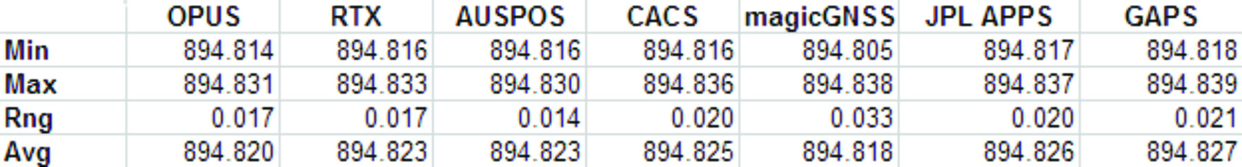
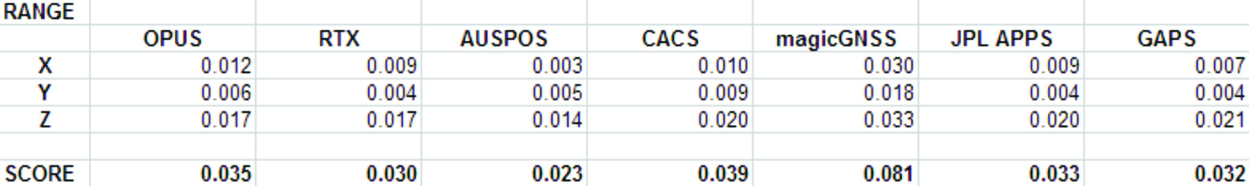
To keep the evaluation simple, the sum of the X, Y and Height range will be the score and the services will be ranked from lowest score to highest score, with the low score being the ‘best.’
Range was chosen as an indicator of the expected maximum error that might be encountered if only a single 24-hour file was observed.
The combined range rewards a processing scheme that best estimates delays, interference, clock errors and other sources of change that occurred during the 32-day trial.
Remember that the every aspect of this ‘competition’ is arbitrary: from the selection of observation sets, to the final scoring system.
The real take-away from this evaluation is not that one service is better, but how close all of the services are to each other.
Two services (JPS’s APPS, magicGNSS) won’t be acceptable to the average user and a third (RTX Centerpoint) may not work for some users based on receiver and antenna support. Details of these problems are presented with the service descriptions below.
The Test Data
SGU1 in St. George, UT USA was chosen as the observation base. The observations consist of 32 consecutive days (May 3, 2013 through June 3, 2013), 24-hour observation files, 30-second interval, GPS only data. The data files were downloaded from the NGS CORS archive.
Each of the 32 files were submitted to each of the processing services and the results have been tabulated for X, Y and Ellipsoid Height. All data is presented in IGS08 current epoch framed coordinates. All data has been projected to UTM Meters for these comparisons.
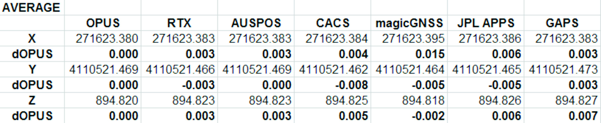
The Average Values
Remember, the real story is how close each of these services produce results to one another. Let’s look at the average positions from each service and the difference from OPUS:
Fig 1: Average Solution Difference from OPUS
As you can see in Figure 1 above, the services were generally within 5mm of OPUS in X, Y and Height.
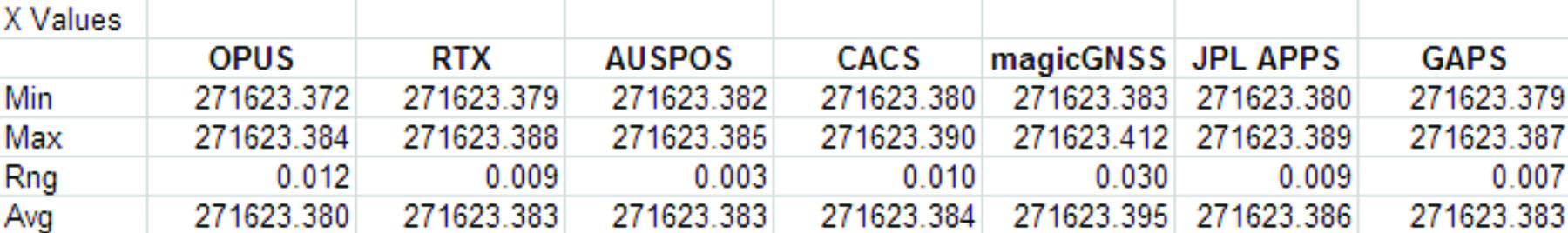
Position Tracking vs. Time
Fig 2: Service Results X vs. Time
Fig 3: Service Results X Range, Average
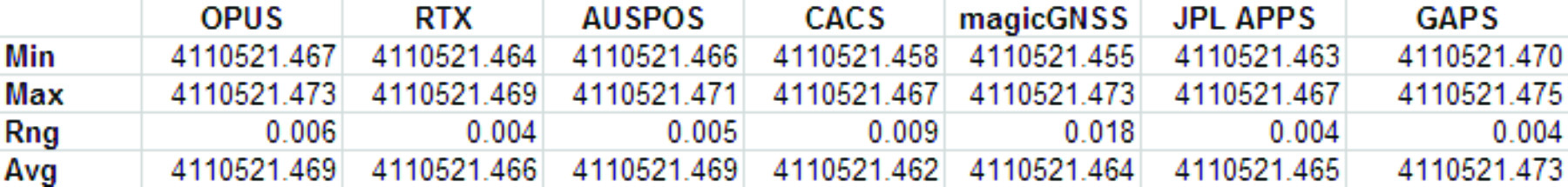
Fig 4: Service Results vs. Time
Fig 5: Service Results Y Range, Average
Fig 6: Service Results Z vs. Time
Fig 7: Service Results Z vs. Time
And the Winner Is…
Following are the scores, based on the combination of X, Y and Height range:
Fig 8: The Scores
Score ranking (remember this is just for fun as the services provided remarkably similar results):
AUSPOS
CenterPointRTX
GAPS
APPS
OPUS
CSRS-PPP
magicGNSS
There is a significant issue in the JPL APPS’s reported output positions, which will keep it from being of any use to most users. magicGNSS’s results are significantly different than the other services. User’s should independently evaluate magicGNSS’s suitability for their purpose. SOPAC’s SCOUT could not be evaluated because it patently does not support either the receiver or antenna that was used at the test site.
AUSPOS is a free service from Geoscience Australia. Access is via a simple web interface, the antenna height and type are entered along with a email address for the returned report set. File submission is via FTP or directly from the web interface.
The returned PDF report is the best looking of the reviewed services and includes a Processing Summary showing a map of the CORS sites that were used in the solution. SINEX files are also available.
AUSPOS uses the Bernese GNSS Software for processing baselines, IGS orbits and IGS network stations. Solutions are available for anywhere on the earth.
RINEX files need to be at least 1-hour in length, 6-hour files are recommended. Compact RINEX files are also accepted. Files may be compressed with UNIX, Hatanaka, ZIP, gzip or bzip compression.
Centerpoint RTX Post Processing: Trimble Navigation Limited
CenterPoint RTX Post Processing is a free service offered by Trimble.
It works anywhere in the world and is based on a proprietary Trimble 100+ worldwide CORS network. Accuracy is 2 cm with 1-hour of observation data; 1 cm with 24-hours. Files longer than 24-hours are not accepted.
RTX uses GPS, GLONASS and QZSS tracked SV’s.
The reported output frames include ITRF2008 at current epoch and a user selectable frame like NAD83/2011 2010.0. RTX is one of the few services that will directly export NAD83 framed results.
A single page PDF and a XML result file are returned by RTX. Unfortunately, it is not possible to copy numerical results from the read-only PDF result file to the clipboard.
RTX supports a limited number of receivers (Trimble) and a relatively small subset of IGS modeled antennas. For this test, TEQC was used to stuff the RINEX headers with a comparable Trimble receiver to the actual Ashtech ProFlex 500 receiver that is in use at SGU1. This was all that was required to spoof an accepted device. If the antenna had not been listed, it would have been necessary to spoof the antenna and adjust the height to reflect the difference in L1 phase center offset.
GAPS is an ongoing project at the University of New Brunswick and was developed by the Department of Geodesy and Geomatics Engineering.
File submission is by a web page and GAPS provides a large number of user inputs and potentially allows the highest level of customization of any of the reviewed services:
You may enter a priori coordinates, and a priori constraints
GAPS accepts static or kinematic files
You can set the elevation mask
The Neutral Atmosphere Delay model is selectable
Earth Body Tides and Ocean Tidal Loading can be applied or disabled
GAPS only processes GPS data (no GLONASS.)
Submitted filenames must adhere to the SSSSDDDh.YYt file format. GAPS accepts RINEX and compact RINEX files, they may optionally be gzip, unix compressed or ZIP compressed.
WARNING! APPS only reports the derived position to the nearest decimeter-meter in geographic (lat/lon) coordinates, while reporting ECEF coordinates to a fraction of a millimeter. If you choose to use APPS, you will need to manually convert the ECEF XYZ to geographic coordinates.
JPL’s APPS is based on GIPSY-OASIS (currently version 5). APPS uses NASA’s 70+ Global GPS Network plus densification from other systems (100+ total receivers distributed globally.) Solutions are typically available with 5 seconds delay from observation.
APPS is easy to use, you just specify a file to upload and then click on ‘Upload’ it takes only 15 seconds to get a result after the file upload is complete. You can optionally register for a free account and use email or FTP for bulk uploads.
APPS also has receiver Live Performance Monitoring: (http://www.gdgps.net/monitoring/index.html) which generates a real time graph of three receivers spread through the world.
Before using CSRS-PPP, you will need to register for a free user account.
CSRS has a fantastic desktop application named PPP-Direct that you can just drag and drop files onto. PPP-Direct automatically submits the file and saves all typing, greatly reducing the chance of error.
CSRS-PPP uses both GPS and GLONASS (if available) observables. Ocean Title Loading corrections can be overridden.
CSRS-PPP will accept single frequency files for processing. CSRS will accept RINEX and Compact RINEX, and will decode ZIP, GZIP and unix compression formats.
CSRS-PPP has a fantastic PDF report, a .csv file detailing results epoch by epoch and a great machine readable summary file.
The desktop submission tool, coupled with the great output reports made CSRS-PPP my favorite tool.
magicGNSS accepts emailed files and returns solutions by email. Turnaround time is fast and features a nice PDF report plus SINEX, receiver clock bias files, tropospheric delay, KML trajectory and RINEX CLK clock bias files.
Static and kinematic files with observations from GPS, GLONASS are processed by magicGNSS and the service reportedly Galileo-ready.
magicGNSS uses a subset of IGS stations to provide core coverage.
SCOUT: Scripps Orbit and Permanent Array Center (SOPAC). University of California, San Diego
Scout accepts RINEX and compact RINEX files, compressed (Z, gz, ZIP) submitted from an FTP site or pushed onto a provided FTP server.
Files must be generated on a limited subset of receivers and antennas. While the IGS antenna and receiver files are the basis for acceptable devices, not all IGS-listed devices are on the allowable device list. SCOUT documentation specifically warns against spoofing devices and antennas.
SCOUT uses the GAMIT processing engine.
Because the test data for this article is from a unsupported receiver and the submittal process requires a FTP host server with anonymous access which most users will not bother with, the output from SCOUT was not evaluated.
Conclusion
The similarity of results between all of the services I processed is amazing. That they differ only by millimeters demonstrates the robustness of the algorithms and processes they use.
The difference between AUSPOS, RTX, GAPS, OPUS and CSRS-PPP solutions are negligible. For important positioning projects, it undoubtedly makes sense to use them all.
For locations in the United States, OPUS and RTX return NAD83-2011 framed results. Only OPUS returns derived orthometric heights using GEOID12A. While OPUS has more provenance than the other services, it is easy enough to submit important observations to multiple services as a reality check for important positions.
###
As you read from Mark’s report above, even though OPUS is shut down until the U.S. Congress can resolve its differences, don’t let that stop you from processing your GPS static sessions. However, some level of due diligence on your part is needed as requirements vary for each service. For example, static sessions for the OPUS-RS service can be as short as 15 minutes while other services require two hour GPS static sessions. Furthermore, some services process GPS L1 data while others require both GPS L1 and GPS L2 observations.
On October 1, 2013, the U.S. federal government shut down and furloughed 800,000 non-essential workers. While services considered essential remained active, those considered non-essential services, like the National Geodetic Survey’s Online Positioning User Service (OPUS), were shutdown. OPUS is a free, online GPS post-processing service. If you try to access www.ngs.noaa.gov, the following screen will be displayed:
Photo: NOAA
For those of you who rely on OPUS for GPS post-processing, now is a great time to try one of the other seven online post-processing services available and not subject to the U.S. federal government. Yes! I wrote seven, and the results from those seven are comparable to OPUS. The other seven, free online GPS post-processing services are:
CSRS-PPP: Canadian Spatial Reference System, Natural Resources Canada
My colleague Mark Silver, creator of the X90-OPUS receiver I wrote about a few months ago, embarked on an effort to run test data through each of the online post-processing services to demonstrate that there are free, online GPS post-processing services available worldwide that produce results comparable to OPUS. The following report is the result of his efforts:
A Comparison of Free GPS Online Post-Processing Services
By Mark Silver
You are probably familiar with the National Geodetic Survey’s OPUS suite of online post processing tools (OPUS-Static, OPUS-Rapid Static and OPUS-Projects.) These services are capable of producing centimeter-level positioning from static GPS observations. What you may not realize is there are at least six viable alternatives to OPUS.
All are free, easy to use, provide world-wide coverage, and generate surprisingly similar results.
Since each uses a unique baseline tool and processing strategies they form an excellent reality check against each other.
IGS orbits and the IGS permanent CORS arrays are used by many of the services, however some use proprietary equipment arrays and orbit products that provide additional redundancy.
How comparable are these services? Which one is the best?
Criteria for Comparing
Comparing results is a difficult proposition:
The true/correct answer for any site is unknown.
What grading scale should be used? Should elevation differences be weighted differently than horizontal differences?
Should the peak-to-peak range or the standard-deviation be prized?
Should comparisons be made on long 24-hour data sets or short 2-hour occupations?
Is a single data set sufficient for a meaningful comparison or are multiple data sets preferable?
Should a service be ‘thrown out’ of consideration because the solutions are substantially different from the mean?
The answer to all of these questions is “it depends.” Your evaluation will depend on your specific application.
For this evaluation, the following rules governed the data set selection:
Choose a site known to be stable with a clean EMI environment.
Use 24-hour observation sets to enable ‘best case’ processing.
Use a sufficiently large data set, 32-consecutive days, to expose trends.
Choose a time period, 90-days in the past, so precise orbits are available to reduce ephemeris effects.
Only consider GPS data.
Use default settings for every option on each processing service.
Scoring
This would not be as interesting without a little competition.
To keep the evaluation simple, the sum of the X, Y and Height range will be the score and the services will be ranked from lowest score to highest score, with the low score being the ‘best.’
Range was chosen as an indicator of the expected maximum error that might be encountered if only a single 24-hour file was observed.
The combined range rewards a processing scheme that best estimates delays, interference, clock errors and other sources of change that occurred during the 32-day trial.
Remember that the every aspect of this ‘competition’ is arbitrary: from the selection of observation sets, to the final scoring system.
The real take-away from this evaluation is not that one service is better, but how close all of the services are to each other.
Two services (JPS’s APPS, magicGNSS) won’t be acceptable to the average user and a third (RTX Centerpoint) may not work for some users based on receiver and antenna support. Details of these problems are presented with the service descriptions below.
The Test Data
SGU1 in St. George, UT USA was chosen as the observation base. The observations consist of 32 consecutive days (May 3, 2013 through June 3, 2013), 24-hour observation files, 30-second interval, GPS only data. The data files were downloaded from the NGS CORS archive.
Each of the 32 files were submitted to each of the processing services and the results have been tabulated for X, Y and Ellipsoid Height. All data is presented in IGS08 current epoch framed coordinates. All data has been projected to UTM Meters for these comparisons.
The Average Values
Remember, the real story is how close each of these services produce results to one another. Let’s look at the average positions from each service and the difference from OPUS:
Fig 1: Average Solution Difference from OPUS
As you can see in Figure 1 above, the services were generally within 5mm of OPUS in X, Y and Height.
Position Tracking vs. Time
Fig 2: Service Results X vs. Time
Fig 3: Service Results X Range, Average
Fig 4: Service Results vs. Time
Fig 5: Service Results Y Range, Average
Fig 6: Service Results Z vs. Time
Fig 7: Service Results Z vs. Time
And the Winner Is…
Following are the scores, based on the combination of X, Y and Height range:
Fig 8: The Scores
Score ranking (remember this is just for fun as the services provided remarkably similar results):
AUSPOS
CenterPointRTX
GAPS
APPS
OPUS
CSRS-PPP
magicGNSS
There is a significant issue in the JPL APPS’s reported output positions, which will keep it from being of any use to most users. magicGNSS’s results are significantly different than the other services. User’s should independently evaluate magicGNSS’s suitability for their purpose. SOPAC’s SCOUT could not be evaluated because it patently does not support either the receiver or antenna that was used at the test site.
AUSPOS is a free service from Geoscience Australia. Access is via a simple web interface, the antenna height and type are entered along with a email address for the returned report set. File submission is via FTP or directly from the web interface.
The returned PDF report is the best looking of the reviewed services and includes a Processing Summary showing a map of the CORS sites that were used in the solution. SINEX files are also available.
AUSPOS uses the Bernese GNSS Software for processing baselines, IGS orbits and IGS network stations. Solutions are available for anywhere on the earth.
RINEX files need to be at least 1-hour in length, 6-hour files are recommended. Compact RINEX files are also accepted. Files may be compressed with UNIX, Hatanaka, ZIP, gzip or bzip compression.
Centerpoint RTX Post Processing: Trimble Navigation Limited
CenterPoint RTX Post Processing is a free service offered by Trimble.
It works anywhere in the world and is based on a proprietary Trimble 100+ worldwide CORS network. Accuracy is 2 cm with 1-hour of observation data; 1 cm with 24-hours. Files longer than 24-hours are not accepted.
RTX uses GPS, GLONASS and QZSS tracked SV’s.
The reported output frames include ITRF2008 at current epoch and a user selectable frame like NAD83/2011 2010.0. RTX is one of the few services that will directly export NAD83 framed results.
A single page PDF and a XML result file are returned by RTX. Unfortunately, it is not possible to copy numerical results from the read-only PDF result file to the clipboard.
RTX supports a limited number of receivers (Trimble, Ashtech, Javad, some Leica, some Topcon) and a relatively small subset of IGS modeled antennas. For this test, TEQC was used to stuff the RINEX headers with a comparable Trimble receiver to the actual Ashtech ProFlex 500 receiver that is in use at SGU1. This was all that was required to spoof an accepted device. If the antenna had not been listed, it would have been necessary to spoof the antenna and adjust the height to reflect the difference in L1 phase center offset.
GAPS is an ongoing project at the University of New Brunswick and was developed by the Department of Geodesy and Geomatics Engineering.
File submission is by a web page and GAPS provides a large number of user inputs and potentially allows the highest level of customization of any of the reviewed services:
You may enter a priori coordinates, and a priori constraints
GAPS accepts static or kinematic files
You can set the elevation mask
The Neutral Atmosphere Delay model is selectable
Earth Body Tides and Ocean Tidal Loading can be applied or disabled
GAPS only processes GPS data (no GLONASS.)
Submitted filenames must adhere to the SSSSDDDh.YYt file format. GAPS accepts RINEX and compact RINEX files, they may optionally be gzip, unix compressed or ZIP compressed.
WARNING! APPS only reports the derived position to the nearest decimeter-meter in geographic (lat/lon) coordinates, while reporting ECEF coordinates to a fraction of a millimeter. If you choose to use APPS, you will need to manually convert the ECEF XYZ to geographic coordinates.
JPL’s APPS is based on GIPSY-OASIS (currently version 5). APPS uses NASA’s 70+ Global GPS Network plus densification from other systems (100+ total receivers distributed globally.) Solutions are typically available with 5 seconds delay from observation.
APPS is easy to use, you just specify a file to upload and then click on ‘Upload’ it takes only 15 seconds to get a result after the file upload is complete. You can optionally register for a free account and use email or FTP for bulk uploads.
APPS also has receiver Live Performance Monitoring: (http://www.gdgps.net/monitoring/index.html) which generates a real time graph of three receivers spread through the world.
Before using CSRS-PPP, you will need to register for a free user account.
CSRS has a fantastic desktop application named PPP-Direct that you can just drag and drop files onto. PPP-Direct automatically submits the file and saves all typing, greatly reducing the chance of error.
CSRS-PPP uses both GPS and GLONASS (if available) observables. Ocean Title Loading corrections can be overridden.
CSRS-PPP will accept single frequency files for processing. CSRS will accept RINEX and Compact RINEX, and will decode ZIP, GZIP and unix compression formats.
CSRS-PPP has a fantastic PDF report, a .csv file detailing results epoch by epoch and a great machine readable summary file.
The desktop submission tool, coupled with the great output reports made CSRS-PPP my favorite tool.
magicGNSS accepts emailed files and returns solutions by email. Turnaround time is fast and features a nice PDF report plus SINEX, receiver clock bias files, tropospheric delay, KML trajectory and RINEX CLK clock bias files.
Static and kinematic files with observations from GPS, GLONASS are processed by magicGNSS and the service reportedly Galileo-ready.
magicGNSS uses a subset of IGS stations to provide core coverage.
SCOUT: Scripps Orbit and Permanent Array Center (SOPAC). University of California, San Diego
Scout accepts RINEX and compact RINEX files, compressed (Z, gz, ZIP) submitted from an FTP site or pushed onto a provided FTP server.
Files must be generated on a limited subset of receivers and antennas. While the IGS antenna and receiver files are the basis for acceptable devices, not all IGS-listed devices are on the allowable device list. SCOUT documentation specifically warns against spoofing devices and antennas.
SCOUT uses the GAMIT processing engine.
Because the test data for this article is from a unsupported receiver and the submittal process requires a FTP host server with anonymous access which most users will not bother with, the output from SCOUT was not evaluated.
Conclusion
The similarity of results between all of the services I processed is amazing. That they differ only by millimeters demonstrates the robustness of the algorithms and processes they use.
The difference between AUSPOS, RTX, GAPS, OPUS and CSRS-PPP solutions are negligible. For important positioning projects, it undoubtedly makes sense to use them all.
For locations in the United States, OPUS and RTX return NAD83-2011 framed results. Only OPUS returns derived orthometric heights using GEOID12A. While OPUS has more provenance than the other services, it is easy enough to submit important observations to multiple services as a reality check for important positions.
###
As you read from Mark’s report above, even though OPUS is shut down until the U.S. Congress can resolve its differences, don’t let that stop you from processing your GPS static sessions. However, some level of due diligence on your part is needed as requirements vary for each service. For example, static sessions for the OPUS-RS service can be as short as 15 minutes while other services require two hour GPS static sessions. Furthermore, some services process GPS L1 data while others require both GPS L1 and GPS L2 observations.
Effigis today announced the worldwide availability of a new version of its OnPOZ EZSurv GNSS post-processing software (V2.92). Improvements include automatic access to data from more than 8,000 base stations around the world and availability of more than 750 mapping systems, as well as enhanced compatibility with 22 native GNSS formats.
EZSurv, Effigis’ GNSS post-processing software, provides a reliable, efficient RTK offline solution to improve survey or GIS data accuracy, the company said. EZSurv is fully compatible with most industry-standard field survey and GIS data collection software.
The latest version of EZSurv offers easy, automatic access to base station providers worldwide: data from more than 8,000 stations around the world can be automatically accessed directly through the EZSurv interface, without any extra user intervention, the company said.
Effigis constantly works on bringing data from more base stations to EZSurv users to improve worldwide connectivity to regional reference frames. “We regularly implement compatibility with additional base station providers as we get the necessary technical information,” said Denis Parrot, president of Effigis. Once compatibility is established, all necessary information to access new base stations is automatically updated through the Internet, without any software release or update.
This latest release also integrates compatibility with new GNSS binary formats, which brings EZSurv compatibility to 22 native formats.
Finally, EZSurv now offers more than 750 predefined “Map Projections/Datums” to help users quickly translate GNSS positions into regional mapping systems. This predefined map projection set is continuously updated on users’ desktops by a simple Internet download.
“EZSurv V2.92 brings GNSS post-processing to an unprecedented level of ease of use,” added Denis Parrot. “EZSurv is a real gateway to many GNSS networks worldwide and provides post-processed results in the proper reference frames. Our commitment to streamline GNSS post-processing makes EZSurv the ideal tool to complement RTK systems.”
Last week, I conducted a webinar along with Dr. Michael Whitehead titled “SBAS, DGPS or Post-processing? Which Should You Use?” It was one of the best webinars I’ve conducted to date. More than 600 people registered. We barely squeezed it into 65 minutes and could have kept going for the better part of two to three hours, given the subject matter to cover and the number of questions we received before and during the webinar. Thank you for attending, if you did. If you weren’t able to you, can download it by registering here. After registering, you’ll be provided a link to download it.
I knew that only having 65 minutes would be a serious issue for the webinar because the discussion could take many worthwhile tangents. And it was. But alas, we stuck to the presentation agenda, stayed on schedule, and were able to address several audience questions.
We had a lot of questions before and during the webinar. As customary, I’d like to address some of those as well as present the poll results here. First, the poll questions and results with accompanying pie charts to illustrate the results.
Poll #1: For those of you who use post-processing, what are the reasons you use it?
Total votes: 117
Gakstatter comment: This is an interesting spread with no clear dominating reason. Based on data I’ve seen and data we collected, I’m not convinced that post-processing is more accurate. If it is, is it worth the extra 10%, 20%, or ??% accuracy? I understand the votes for more reliable corrections. There’s something to say for reverse processing (forwards and backwards).
Poll #2: For those of you using post-processing, from where do you access GPS base station data?
Total votes: 129
Gakstatter comment: These answers don’t surprise me. National and regional CORS have become very prolific in the past 10 years.
Poll #3: For those of you who use real-time DGPS/SBAS, what is the reason you use it?
Total votes: 110
Gakstatter comment: These answers surprised me a little. I thought more people would vote for “less complicated.” Does that percentage of users really need corrected coordinates in the field? Why? E-mail me a quick answer if you have a chance.
Poll #4: For those of you using real-time DGPS/SBAS, from where do you access DGPS/SBAS corrections?
Total votes: 129
Gakstatter comment: This answer doesn’t surprise me at all. I suspect RTK networks will increase due to their continued proliferation and different levels of accuracy offered.
Poll #5: When I purchase GPS/GNSS equipment in the future, I will likely select equipment that utilizes the following correction method (select all that apply):
Total votes: 144
Gakstatter comment: This was the only multi-answer poll. People could select more than one answer. These answers were surprisingly close. That surprised me. It didn’t surprise me that SBAS was the leader. It surprised me that post-processing is still as predominant as it is. If you have a chance, e-mail me a quick explanation as to why you will use post-processing in the future.
Before diving into some audience questions, I’d like to clarify the slide illustrating the post-processing plot shown below.
During the webinar, we were discussing PPP (precise-point positioning) when this slide was displayed. This data was not corrected via PPP, but rather post-processing the pseudorange data, which is the equivalent of L1 SBAS and L1 DGPS. The point was to show how SBAS/DGPS accuracy compares to post-processing. In the real world, you won’t post-process 24 hours of data. Some of you will post-process only a few minutes of data per session in cases where you need to turn off the receiver and travel between points. In other cases, users will keep the receiver tracking between points, allowing reverse processing to work more effectively.
On to the Questions
Question #1: Will there ever be a way in which the position of a rover can become fixed by using two fixed base stations?
Gakstatter comment: SBAS does this already. SBAS’s consist of a number of base stations within the coverage area (e.g., WAAS has 38). Data from many base stations is used to compute the correction information sent to an SBAS-enabled GPS receiver.
I’m assuming your reasoning is to improve position integrity.
Another method of accomplishing this is by post-processing against more than one base station or switching between DGPS beacon stations. If they differ significantly, then you might want to compare against a third base station.
Question #2: At what point in time will the strength of the GPS signal be increased? To what strength will this occur? 500 times more powerful? What improvements in signal reception will be experienced? Indoor my house reception?
Gakstatter comment: The GPS broadcast strength is increased with new GPS satellite model. For example, the current Block IIF satellite broadcasts the new L5 signal about four times stronger than L2C. While no one can be sure yet as to how much this will improve indoor positioning, there will be some marginal improvement in conditions where GPS doesn’t operate very well today. Also helping will be the improved code and error-correcting techniques that should make operating in difficult conditions a bit better, especially where there are a mixture of satellites with strong and weak signals.
Also, it raises the issue of a viable L5 single frequency receiver, which should outperform the L1 C/A single frequency receivers of today.
Question #3: NAD83, WGS84, ITRF differences, how to make the best choice?
 
;
Gakstatter Comment: I don’t think there is an incorrect choice, except maybe that NAD83 is a 2D system and will eventually give way to a 3D system, but that won’t happen in the U.S. for many years.
Otherwise, it’s a question of matching disparate data sets. Probably the #1 question I hear from users is “why doesn’t my GPS data line up with my basemap?” The answer is almost always a difference in datums. Many papers have been written on this. Click here for a good PowerPoint presentation created by Dave Doyle of the National Geodetic Survey.
Question #4: Are there any open source post-processing software programs available?
Question #5: If a person uses real-time correction satellites, is there a need to post-process?
Gakstatter Comment: It’s rare that someone would do both, but not out of the question. For example, one might rely primarily on real-time corrections and record raw data for post-processing in case there is a problem receiving the real-time corrections. The opposite is true, too. One might rely primarily on post-processing and use real-time corrections as a back-up in case there is a problem with post-processing.
Caveat emptor: There are probably datum differences between the sources of real-time and post-processing corrections. This needs to be reconciled when combining data that has used the two sources.
Question #6: Is it possible to post-process data without using a DGPS?
Gakstatter Comment: Yes, all that is required for post-processing is the ability to record raw observation data.
Question #7: Are there geographic areas in the U.S. that are not covered by NGS CORS stations?
Gakstatter Comment: No, not for pseudorange (L1) differential corrections. The distance to the base station will vary depending on where you are located and thus may affect your accuracy to some degree, but the density of CORS in the U.S. is such that you will never be more than a couple of hundred kilometers from a base station and likely much closer.
A side note: Back in the mid-1990s, I remember experimenting with post-processing software we were developing. At that time, I tried post-processing data collected in Oregon with a base station located in Atlanta, Georgia. This was a 2,500 km baseline. It produced a result, albeit not one I would necessarily trust. The only limitation is that the two units must track common GPS satellites. With that length of baseline, it’s possible that only half of the satellites tracked may be in common.
Question #8: What is the ideal distance range from a CORS station to your site to use post-processing?
Gakstatter Comment: Ideally, as close as possible. The further you are from a base station, the more potential error will be introduced due to atmospheric differences between the two locations. As stated above, the density of CORS (at least in the U.S. and many parts of the world) are such that the nearest base station is quite near and likely no more than a couple of hundred kilometers away.
Question #9: What is the trade-off between short observation time (couple of minutes) to position accuracy when using post-processing?
Gakstatter Comment: Ok, remember we are talking about pseudorange corrections (as opposed to carrier phase). Given that the receiver has been tracking satellites for a period of time (let’s say two minutes), the observation times only need to be a few seconds for each feature to be mapped.
For example, if you are mapping utility poles and don’t turn off the receiver between poles, you only need a few seconds (5-10 seconds) of data for each pole and average it for the final coordinate. Think about if you’re mapping a road centerline. You’ll likely record data while moving, so each second you are recording a new position.
Question #10: What about the vertical correction? I see in the slide an antenna carried in a backpack. Is the antenna placed at ground level for point? Is there a constant correction required?
Gakstatter Comment: Vertical accuracy is typically worse than horizontal accuracy by a factor of 1.5-2.0 due to the inferior satellite geometry, especially in areas of hilly terrain and/or trees/buildings where the horizon is blocked. Good geometry for vertical positioning requires tracking a number of GPS satellites that are low on the horizon.
Question #11: What is the future of DGPS? I heard Coast Guard beacons were going away?
Gakstatter Comment: The beacon stations operated by the U.S. Coast Guard are not in jeopardy and never have been. Neither have the marine beacons in the other 40+ countries that broadcast GPS corrections. However, the U.S. Department of Transportation operates 29 inland stations in the U.S. which have faced budget challenges the past few years. In April 2008, the U.S. DOT issued a policy decision to continue operating the 29 inland sites. Construction of seven sites remains that would allow the Nationwide DGPS to reach Initial Operating Capability (IOC), which would provide coverage to 99% of the continental U.S. No budget has been approved for the construction of those seven sites.
Question #12: Can you briefly explain the difference between DGPS & RTK?
Gakstatter comment: Here are a couple of good websites that explain each of these techniques. Essentially, DGPS is a real-time GPS positioning technique accurate to about 30 centimeters at the very best. RTK is a real-time GPS positioning technique accurate to about 1 centimeter.
Question #13: How much time do you need to get the position from the base station for real-time DGPS?
Gakstatter comment: Assuming both receivers are already tracking satellites, your receivers will begin using the base-station corrections as soon as the data link is made between the two.
Question #14: Can you comment on advantages (if any) of using corrections from a network RTK service for DGPS corrections. Any advantages on eliminating base separation?
Gakstatter comment: I’ve heard that DGPS corrections are optimized within an RTK Network. However, I need to research this a bit further to better understand the true advantages, if any.
Whitehead Comment: A virtual base station (VBS) solution could be formed using the network. Thus differential GPS could exhibit the same advantages using such a network that RTK does (cancellation of atmosphere errors). The software would have to support this.
Note though that if close to one of the Reference Stations in the network, it is probably best to just use the nearest Reference station as this will best cancel the atmosphere errors. When in the middle the network, the VBS solution would use surrounding reference stations to provide a good approximation of atmospheric errors and then output a correction that looked like it originated from a reference station (virtual station ) near to the users receiver.
Question #15: What is up with PRN 135? Still on station?
Gakstatter comment: Communication has be re-established with WAAS PRN 135 and is being tested by its owner, Intelsat, as well as the Federal Aviation Administration (FAA). See a detailed article by clicking here. The latest information I heard is that it’s currently at 93°W longitude undergoing testing. If the testing is successful, it will be re-located back to 133°W longitude and brought back into WAAS service. A timeline has not been published, but I’m guessing within the next 30-60 days.
Question #16: We used to hear that your point accuracy degraded as the distance from the base station increased. One reason we used to post process. Is this still a factor?
Gakstatter Comment: Due to advancements in GPS technology, it’s not as much of an issue as it used to be. I think this is illustrated in the results we achieved in our 24 hr test data.
Ten years ago, it would be hard to find a GPS L1 receiver that would receive DGPS corrections from a beacon station 184km away and still achieve sub-meter horizontal accuracy at the 95% confidence level.
I’m not saying the distance is negligible. There still the issue of tropospheric, ionospheric and satellite orbit errors as you move farther away from the base station. But, it’s certainly less of a factor than it was before.
Whitehead Comment:
Question #17: If we use WAAS correction, does it really help to try to use a post-processing type of software afterward? So far we just use WAAS correction.
Gakstatter Comment: One of the reasons we collected data using several sources of real-time corrections and also showed the results of post-processing was to illustrate the differences between the two.
If you follow proper procedures, there’s no reason to think that accuracy obtained using WAAS will differ significantly from accuracy obtained using post-processing. This is assuming that you’re using a single-frequency GPS receiver and post-processing using pseudorange corrections and not carrier-phase processing. Some receivers like the Trimble GeoXH are actually dual-frequency receivers and so data from it will likely surpass the accuracy of WAAS if you’re using its dual-frequency antenna and equivalent post-processing software.
By proper WAAS procedures, I mean letting it track for five minutes upon initial start-up to allow it to download a current ionospheric map.
Question #18: Does SBAS use 1 receiver and no base station? Expensive?
Gakstatter Comment: SBAS uses 1 receiver and a lot of base stations. You just don’t have to pay for the SBAS base stations (or to use them.) The signal, like GPS, is provided free of charge.
SBAS consists of a network of base stations (WAAS has 38) and communications satellites that broadcast corrections to users on the ground (or aviation users in the air).
Question #19: How far north in Alberta is WAAS coverage available and useful?
Gakstatter Comment: The primary concern would be visibility of the WAAS GEO satellite that broadcasts the correction data. Following is a map that illustrates the coverage. The contour lines are degrees above the horizon for which the two WAAS GEO satellites are visible.
Solid line = PRN 138, Dashed line = PRN 133
Question #20: Do you have any comments about CDGPS in Canada/US?
Gakstatter comment: Sadly, the CDGPS service is being decommissioned March 31. You can read about it here.
Question #21: I am hearing from my state specialists (NRCS) regarding the LightSquared issue. We are advising working through the PNT ExComm and our cooperating partners.
Gakstatter comment: This is a potentially serious issue for GPS users. Click here for the latest news as of February 1.
Question #22: Where do you find the DGPS beacon station list and what is available to you?
Gakstatter comment: I’m not sure if this is 100% complete, but it’s the most complete list I’ve seen. Click here.
Question #23: Are most mapping-grade GPS receivers (for example Trimble GeoXh) equipped off the shelf to receive beacon signals?
Gakstatter comment: Some receivers are equipped off-the-shelf, others are not (such as the GeoXH) and require additional hardware.
Question #24: In which areas is it possible to use corrections from OmniSTAR?
Gakstatter comment: Click here to view worldwide maps of OmniSTAR coverage.
Question #25: Was the Garmin set to WAAS?
Gakstatter comment: Yes, during the 24-hour data collection session, the Garmin unit was receiving WAAS 100% of the time as far as we could tell. The purpose of the 24-hour test period was to able to randomly sample data during that period to arrive at the accuracy statistics we presented. I randomly sampled the dataset several time
s (averaging 10 seconds worth of positions 200 times) and the results were consistent with what we presented.
Question #26: How does post processing account for ionosphere or troposphere errors if receiver is geographically far away from the base station? If not, does DGPS and WAAS provide better accuracy and integrity?
Whitehead comment: Post Processing using a CORS station would take the nearest station and do differential GPS which cancels common errors in ionosphere and troposphere (ionosphere and troposphere are both temporally and spatially correlated) so if the CORS station is close, there will be good cancellation. If the receiver is far, the algorithms could use a troposphere model to account for the differential troposphere (as was done in the Presentation for BeaconT) and this would probably cancel troposphere so that remaining errors were sub-decimeter level. Differential Ionosphere errors could also be easily modeled with good results. It is likely that the performance could be made to easily surpass SBAS.
DGPS would suffer from the same effects as does post processing, and maybe even more so since a model of differential atmosphere errors is rarely used. SBAS will likely provide better accuracy in situations where you are far from a base station.
Question #27: What is Beacon T?
Gakstatter Comment: While collecting data to present at the webinar, Mike noticed there was a bias in the beacon measurements. The beacon station is located ~184km away at about 7,000 ft elevation while the test site was at about 1,000 ft elevation. Initially, Mike wasn’t modeling the troposphere difference between the base and rover.
To model the troposphere, Mike said he used a troposphere model to figure out troposphere in both locations, and then subtract the two. Although the models are not necessarily that accurate in an absolute sense, the differential tropo between the two locations is fairly accurate using the models. This differential tropo allows the receiver to correct the tropo in the base station differential to make it appear as if it originated in the rover location. Mike said he could’ve done the same for the ionosphere, but he didn’t since that is it usually less of a factor. After using the modified tropo model (Beacon T), the height bias was around 1/2 meter, which could be attributable the ionosphere. The horizontal bias is small, as you can see in the results.
Using this troposphere model resulted in a significant improvement over the original solution.
Question #28: Why is VBS better than WAAS?
Gakstatter Comment: It surprised me too. The receiver used was the same that was used for beacon and WAAS. I contacted OmniSTAR for their opinion.
John Pointon of OmniSTAR responds: “There have been incremental improvements in the VBS service over the years, mostly improvements in modeling and processing. We have added two or three extra reference stations but that hasn’t been the most critical improvement, just helped in some specific areas. These, combined with the relatively benign solar environment, result in VBS accuracy which, although not equivalent to our dual-frequency and multi-system solutions, is consistently better than either Beacon or WAAS.”
Whitehead Comment: In the past, we’ve seen similar performance from both OmniStar VBS and WAAS. Different atmosphere conditions and different locations can affect the performance of both. We’ve seen situations where WAAS is better. It is probably fair to say that OmniStar is more focused on accuracy, whereas WAAS is focused on integrity. It may be wise to do a comparison in the particular area where you operate. Note, however, that in the US, OmniStar is referenced to NAD83 whereas WAAS is references to ITRF so positions reports between the two can differ by several meters.
Question #29: When I look at your scatter plot, I have to ask if short-term point averaging is really effective at achieving more accurate positions?
Gakstatter Comment: I think it’s well accepted that you are wasting time by occupying a point for 180 seconds. That said, there’s something to be said for letting the receiver track satellites for a period of time (1-2 minutes) before storing 5-10 seconds of data. Of course, if the receiver is already tracking satellites, then it’s not necessary to wait. The idea is to let the measurements settle down and take advantage of carrier-phase smoothing if the receiver uses that technique.
Question #30: Could you go into PPP a bit more? How does it work?
Gakstatter Comment: We opened a can of worms by discussing PPP. It’s an entirely different subject that I will cover in a future article. In the meantime, you can read Dr. Richard Langley’s article on PPP here.
Question #31: How do you test the accuracy of SBAS collected data?
Gakstatter Comment: In the U.S., it’s easy. Find a local survey mark using the National Geodetic Survey website. Printout the ITRF coordinates of the survey mark. If they aren’t on the datasheet, you can convert from NAD83/CORS96 to ITRF using the HTDP program. Compare the coordinates output by your GPS receiver to the coordinates of the survey mark.
If you’re located outside of the U.S., look for a similar government agency in your country that maintains a record of survey marks. It’s vital that you are comparing coordinates referenced to the same datums.
Question #32: Will there be any disadvantage if we use a EGNOS corrections in Kuwait, if we receive EGNOS?
Whitehead Comment: Kuwait is outside the EGNOS coverage zone, so satellites to the south may not even have Clock and Orbit correctors available, which means the Receiver could not compute a correction for these satellites. Unless the receiver can mix differentially cor
rected ranges with non-differentially corrected ranges, it would likely drop the satellites in the south that had no corrections. This would then reduce PDOP and thus accuracy. Mixing differentially corrected ranges with non-differentially corrected ranges may give worse accuracy than no corrections at all since the SBAS system may have clock or other biases relative to GPS.
By the way, I wish the SBAS providers would get together and share data so that they each could provide world-wide orbits and clocks. Then it would matter less if you were outside the coverage area.
Gakstatter Comment: I’ve heard that EGNOS is planning an expansion to the south and east, so Kuwai may eventually be within the EGNOS coverage footprint. Also, you’ll want to monitor the progress of India’s GAGAN system, which is a similar SBAS. It’s possible you might fall within the GAGAN extrapolated footprint for non-aviation users.
We covered most of the questions posed by the audience. If we didn’t address yours or didn’t provide a complete enough answer for you, please e-mail me and I’ll do my best to answer you.
As I mentioned above, we had quite a few questions about PPP. It’s a technology that’s worthy of further coverage and discussion. Look for a future article on it.
If you’ve been around GPS mapping for any length of time, I’m sure you’ve heard of post-processing, and you may have even experienced it yourself. If you used GPS for mapping in the ’90s, you almost certainly post-processed your data. In fact, sometimes you had to pay for access to GPS base-station data for post-processing. That’s hard to imagine given the widespread, worldwide availability of GPS base-station data on the web today.
SBAS (WAAS/EGNOS/MSAS) didn’t exist, and for real-time corrections and DGPS (beacon) coverage was spotty at best, but real-time commercial DGPS services like OmniSTAR, Landstar, and Satloc were around.
One thing is for sure, no matter what, you have to have some source of corrections to collect GPS data for GIS mapping. It’s commonly referred to as differential GPS correction. Essentially, your GPS receiver needs to reference another GPS receiver (base station) that’s set up on a known position.
Grafnav Post-processing software
There are two primary methods in which to apply a correction to your GPS data: post-processing differential correction and real-time DGPS.
Post-processing
When you’re collecting GPS data that’s going to be post-processed, you need a GPS receiver (and software) that’s going to be able to record satellite observation data. Otherwise, data is collected as one normally would in the field, whether it’s utility poles, manhole covers, road centerlines or polygons of any sort.
The accuracy of the GPS data while you’re in the field is autonomous GPS, so it could be several meters or even ten meters or more. You can’t use this type of method for navigating to a point with any sort of accuracy better than a few meters.
After you’re finished collecting your GPS data for the day, you go back to the office and download your data to your computer. Post-processing requires special software. That software will allow you to search the Internet for the closest GPS base station(s) to use as a source of GPS corrections. In previous years, it was a laborious task to search for GPS base-station data that was recorded the same time as you were in the field (remember UTC vs. local time?). That’s not the case any longer as advanced post-processing software has made this a more automated process. The software will search for the closest base station and automatically select the appropriate files to download.
It takes specialized software and training to utilize post-processing effectively.
Real-time DGPS
This is a method of receiving GPS corrections while you’re in the field. The GPS corrections are applied in real-time so your positioning is accurate. This is useful when you want to navigate to a particular point very accurately. In the 1990s, there were a number of DGPS services, mostly commercial. One would pay a monthly or annual subscription fee to receive the DGPS corrections. During that time, the U.S. Coast Guard started developing a system by which it will install GPS base stations near the major U.S. waterways (coastlines and major rivers). It set up large towers that would broadcast the corrections via 300 kHz radio. Most importantly, it broadcast the corrections free of charge. One only needed a “beacon receiver” to receive the corrections. The system didn’t cover the entire U.S., but it opened the eyes as to what was possible in terms of a regionwide, or nationwide, DGPS network of base stations.
The U.S. Coast Guard concept is still used today in more than 40 countries for DGPS marine navigation. The same GPS correction signal is also used by many people using GPS for mapping.
Around the same time, the Federal Aviation Administration (FAA) began developing a system to improve GPS integrity and accuracy. They called it WAAS (Wide Area Augmentation System). It was the first SBAS in the world and, upon being declared operational in 2003, is in use by thousands of people for GPS mapping. SBAS is a regional system. WAAS only covers North America (U.S., Canada, and Mexico). It has spawned a number of similar and compatible systems such as EGNOS in Western Europe and MSAS in Asia with GAGAN under development in India.
There are several advantages and disadvantages to both post-processing and real-time DGPS for GPS mapping. The primary advantage of post-processing is that you don’t have to worry about a wireless data connection in the field. The primary advantage of real-time DGPS is that you get much better accuracy in the field. There are many other factors you should consider when deciding which method to use.
In fact, I think it’s an interesting enough topic that I’m conducting a webinar later this month that will address both of these methods. I’ve invited Dr. Michael Whitehead to join me. He’s the head technology guy at Hemisphere GPS and has worked extensively developing high performance GPS receivers. He was also the chief architect at Satloc back in the late ’90s.
Eric Gakstatter, Editor, Geospatial Solutions and Survey Scene newsletter &
Dr. Mike Whitehead, VP of Technology at Hemisphere GPS
Event Date: 01/26/2011 10:00 AM Pacific Standard Time, 5 PM GMT
Tens of thousands of users around the world utilize GPS/GNSS receivers for mapping, surveying and navigating. Since autonomous GPS/GNSS typically does not provide the needed accuracy, users must rely on a source of GPS/GNSS corrections. There are three sources of GPS/GNSS corrections available to users who desire reliable GPS/GNSS accuracy in the sub-meter to three meter range: SBAS, DGPS and post-processing. Dr. Michael Whitehead, Chief Scientist at Hemisphere GPS, will join me in presenting a background on the three technologies as well as the strengths and weaknesses of each. I’ve known Mike for a number of years. He was an early innovator in the development of SBAS technology at Satloc as well as SBAS and DGPS receiver technology at Hemisphere GPS. He is one of the leading GNSS engineers in the world. I’m particularly excited about this event and promise a lively discussion that’s full of useful information, data and concepts that anyone using or considering using GPS/GNSS for mapping, surveying or navigating will find useful.


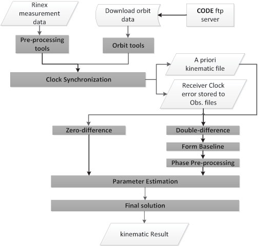
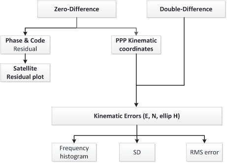
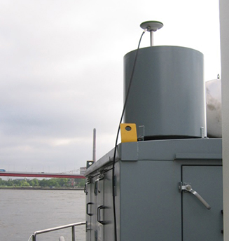
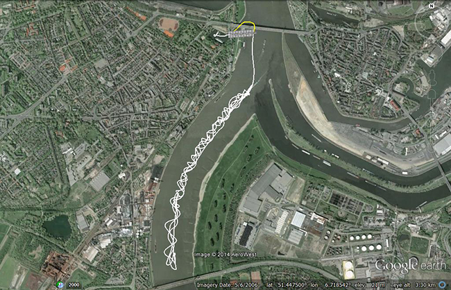
![Figure 3. Layout of the first trajectory [DOY: 2014/126], zoom-in on bottom. (Photo: Google Earth)](https://stage.globalpositioningnews.com/wp-content/uploads/2015/12/Figure-4-W.jpg)
![Figure 4. Satellite residuals for the first trajectory [DOY: 2014/126].](https://stage.globalpositioningnews.com/wp-content/uploads/2015/12/Figure-5-W.jpg)
![Table 1. Statistical results of the first trajectory [DOY: 126/2014].](https://stage.globalpositioningnews.com/wp-content/uploads/2015/12/Table1.jpg)
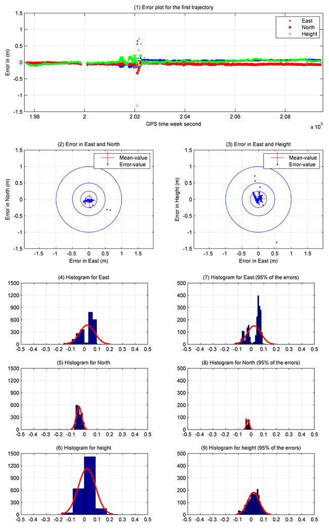
![Figure 6. Layout of the second trajectory [DOY: 127/2014]. (Photo: Google Earth)](https://stage.globalpositioningnews.com/wp-content/uploads/2015/12/Figure-7-W.jpg)
![Figure 7. Satellite residuals for the second trajectory [DOY: 127/2014].](https://stage.globalpositioningnews.com/wp-content/uploads/2015/12/Figure-8-W1.jpg)
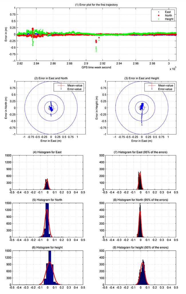
![Table 2. Statistical results of the second trajectory [DOY: 127/2014].](https://stage.globalpositioningnews.com/wp-content/uploads/2015/12/Table2.jpg)