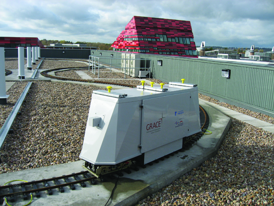
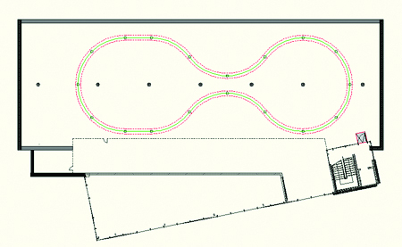
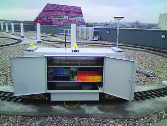
One-hundred-twenty meters of test track, designed for repeatable dynamic position testing, run along the roof of the new Nottingham Geospatial Building at the University of Nottingham, UK. The figure-eight track provides an optimal controlled environment with test equipment aboard a remote-controlled, multi-sensor 7¼-inch gauge locomotive platform with a top speed of 7 kilometers per hour, a dedicated power supply, and five antenna mounts. Simulation of the track using Spirent GSS8000 hardware (GPS and Galileo) provides additional planning and testing capacity.
The combination of these tools creates the ideal environment for our new project: augmentation of GNSS systems with ground-based Locata positioning technology. This pseudolite-like system, described in the March issue of GPS World, works in a GNSS-like fashion, using code and carrier phase. The major advantage, apart from utilization of the licensee-free 2.4 GHz frequency band, is the precise time synchronization of the network to the nanosecond level.
The proposed integration addresses Locata’s weak vertical coordinates (due to relative coplanarity of transceivers) and GNSS’s requirement for a clear view of the sky and location-specific weak geometric distribution of the satellites. Prior research and analysis suggests considerable improvement in 3D positioning accuracy when combining ground-based positioning devices (pseudolites) with GNSS, but the current project pushes the research forward by attempting to create on-the-fly ambiguity resolution.
Combination of hardware and software simulation has provided an initial assessment of the proposed integration, optimization of equipment location, and test of the mathematical model to be used. Practical tests, using the roof lab on top of the NGB, will further verify the method and allow comparisons between the predicted and real-life results. This will aid the assessment of noise, multipath, and in-bound interference. The test design minimizes the tropospheric effect, while track flexibility and repeatability offer the possibility of implementing and simulating obstructions and areas of GNSS outage. This will provide a full assessment of the mathematical model and the integrated system’s capacity.
This project offers new opportunities in civil engineering, specifically monitoring and machine control. GPS is currently widely used for those applications, with Locata also proven successful. The integrated solution can provide not only enhanced positioning capacity but lower the required number of visible GNSS satellites, and offer improved integrity and quality control, ultimately increasing the safety of life.
The intended utilization is for positioning in dense urban areas and essential structures (airports, seaports, factory sites, bridges) where sky visibility or correct satellite distribution cannot be guaranteed.
The track is available for other projects. Funded by East Midlands Development Agency, hosted by the Institute of Engineering Surveying and Space Geodesy, the Centre for Geospatial Science, and the GNSS Research and Applications Centre of Excellence (GRACE).
Testing GNSS Receivers with Record and Playback Techniques
By David A. Hall
Is there a way to perform repeatable tests on GNSS receivers using real signals? This month’s column looks at how to use an RF vector signal analyzer to digitize and record live signals, and then play them back to a GNSS receiver with an RF vector signal generator.
INNOVATION INSIGHTS by Richard Langley
AS A PROFESSOR, I’m quite familiar with testing — of students, that is. It’s how we check their performance — how well they have mastered the course material. Outside academia, testing is also quite common. We have to pass a driving test before we can get a license. We might have to pass a physical fitness test before starting a job. And manufacturers have to test or stress their products to make sure they are fit for purpose. As David Ogilvy, the father of advertising once quipped, “Never stop testing, and your advertising will never stop improving.” But it’s not just manufacturers who should test products. Consumers, or their representatives, should test products on offer — not only to corroborate (or dispute) manufacturers’ claims but also to compare one manufacturer’s product against another. There’s a whole slew of magazines, television programs, and web resources devoted to testing and comparing everything from laundry detergent to automobiles. And GNSS receivers are no exception.
When we conduct tests, we are usually trying to get answers to certain questions — just like those posed to students on their exams. In testing GNSS receivers, what are some appropriate questions? When a receiver is turned on, how long does it take until the position of the receiver is determined? When a weak signal area is encountered, can the receiver still determine its position? If the signal is interrupted and then restored, how long does it take for the receiver to recover and resume calculating its position? And what is the position accuracy under different situations?
While we can certainly hook up an antenna to a receiver to get answers to these questions in a certain environment on a certain day at a certain time with certain signals, the scenario cannot be repeated — not exactly. If we tweak a receiver operating parameter, for example, we don’t know for certain whether any observed change is due to the tweaking or a change in the scenario. We could use a radio-frequency (RF) simulator — a device for mimicking the radio signals generated by the satellites. This would allow us to define scenarios, including receiver trajectories, and to replay them as many times as necessary while varying the operating parameters of the receiver. Or we could modify the scenario from run to run. Such test scenarios could include those difficult to carry out with live signals such as determining how a receiver would perform in low Earth orbit. While extremely useful, these are tests with simulated signals.
Is there a way to perform repeatable tests on GNSS receivers using real signals? In this month’s column, we learn how to use an RF vector signal analyzer to digitize and record live signals, and then play them back to a GNSS receiver with an RF vector signal generator — a procedure we can repeat as often as we like.
While GNSS simulators have long provided the de facto technique for testing GPS receivers, radio frequency (RF) record and playback has emerged as an innovative method to introduce real-world impairments to GNSS receivers. In this article, we will provide a hands-on tutorial on how to test a navigation device using the record and playback technique.
The premise of RF record and playback is to capture GNSS signals off the air with a vector signal analyzer (VSA) and then replay them to a receiver with an RF vector signal generator (VSG). With recorded GNSS signals, one is able to introduce a signal that contains natural impairments — instead of an ideal signal — to the GNSS receiver. As a result, one can observe how a receiver will behave in a real-world environment where interference, multipath fading, and other impairments are present.
A VSA combines traditional superheterodyne radio receiver technology with high-speed analog-to-digital converters and digital signal processors to perform a variety of measurements on complex modulated signals. It is widely used in the telecommunications industry as a test instrument. Digitized signals can be recorded for future analysis. A VSG reverses the process, taking a digital representation of a complex waveform and, using digital-to-analog converters, generating an appropriately modulated RF signal.
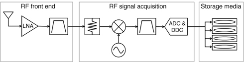
Recording GPS or GLONASS signals off the air can be done in a fairly straightforward manner. An RF recording system combines appropriate antennas, amplifiers, and an RF signal recorder (usually a VSA) to capture many hours of continuous RF signal. In such a system, the basic components include the RF front end, the RF signal-acquisition device, and high-volume storage media. A block diagram of a typical recording system is shown in Figure 1.
Figure 1. GPS receivers implement cascaded low-noise amplifiers. The RF signal acquisition block includes analog-to- digital conversion (ADC) and digital down conversion (DDC) to select the data of interest.
In the figure, the RF front end is designed to condition the GNSS signal in such a way that it can be captured — with maximum dynamic range — by the recording device. The recording device digitizes a given signal bandwidth, and then stores in-phase and quadrature (IQ) waveforms to disk.
In general, RF recording devices are designed to tune to a broad range of frequencies and can thereby record many different types of signals. Thus, selecting the signal to record is as simple as setting the center frequency and bandwidth of the recording device. For example, to record the GPS C/A-code L1 signal, the center frequency should be set to 1575.42 MHz. Because each satellite generates the same carrier frequency, one can capture C/A-code signals from all satellites simply by capturing all signals within a 2.046 MHz (twice the code chipping rate) band around the carrier frequency.
By contrast, recording GLONASS signals requires slightly different settings. Because the GLONASS constellation uses frequency division multiplexing, every satellite generates the same code, but each pair of antipodal satellites transmits at a unique center frequency. Thus, recording L1 signal information for the entire GLONASS constellation requires a recorder to capture signals that range from 1598.0625 MHz (channel -7) to 1605.375 MHz (channel 6). In order to capture the entire bandwidth of each satellite, a recorder is actually required to capture 1.022 MHz of signal for each carrier (again, twice the code chipping rate). Therefore, the total recording bandwidth is actually 1597.5515 MHz to 1605.886 MHz, a span of 10.3345 MHz. On the RF signal analyzer, one can record GLONASS signals simply by setting the center frequency to 1601.71875 MHz, and the bandwidth to ≥ 10.3345 MHz.
Modern RF signal recorders are capable of recording both GPS and GLONASS C/A-code signals on a single wideband recording channel. For example, one of our RF signal analyzers is capable of recording up to 50 MHz of signal bandwidth. With this instrument, one can simultaneously record both GPS and GLONASS by setting the center frequency to 1590.1415 MHz and the bandwidth to ≥ 31.489 MHz. However, while RF recording systems can be used to capture a wide range of GNSS signals including GPS L1/L2/L5, GLONASS L1/L2, Galileo, and others, this article focuses primarily on the GPS C/A-code signal.
Setting up the RF Front End
The trickiest aspect of recording GPS signals is the selection and configuration of the appropriate antenna and low noise amplifier (LNA). When connecting a typical off-the-shelf GPS passive patch antenna to a signal analyzer, the peak power in the GPS L1 band ranges from -120 to -110 dBm. Because the power level of GPS signals is small, significant amplification is required to ensure that the VSA can capture the full dynamic range of the signal.
The simplest method to amplify an off-the-air GPS signal so that it can be captured by an RF signal recorder is the combination of an active GPS antenna and one or more external LNAs. Note that many professional GPS antennas offer the best performance because they combine high element gain with an LNA and even pre-selection filtering, which improves the dynamic range of the RF recorder.
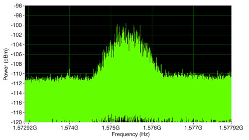
With the RF front end appropriately configured, one can verify system performance using a simple spectrum analyzer demonstration panel. The demo panel allows one to visualize the RF spectrum in the GPS L1 band. If all is set up correctly, the C/A-code GPS signal should be visually present on the display. Figure 2 illustrates a screenshot of the spectrum on a virtual spectrum analyzer display.
Note that visualizing the GPS signal in the frequency domain with an RF signal recorder (or spectrum analyzer) requires careful attention to settings such as resolution bandwidth and averaging. Because the signal-to-noise ratio (SNR) of the GPS signal is so small, the settings shown in Figure 2 require a narrow resolution bandwidth (10 Hz) and significant averaging (20 averages per measurement record, so a 20-second interval for 1 Hz data). With these settings applied, one can easily visualize a modulated signal above the noise floor with approximately 1 MHz of bandwidth and centered at 1575.42 MHz. This signal is the GPS C/A-code. In Figure 2, the reference level of the signal analyzer was set to -50 dBm to reduce the noise floor of the instrument to the lowest possible level. Note that setting the signal analyzer’s reference level provides a simple mechanism to adjust the front-end attenuation or amplification. In general, RF signal analyzers provide the greatest dynamic range when the reference level of the instrument matches closely with the average power of the signal connected to the front end. In this case, setting the reference level of our signal analyzer to -50 dBm removes all front-end attenuation, giving the analyzer a more optimal noise figure for signal recording.
Figure 2. GPS is visible in the spectrum only if a narrow resolution bandwidth is used. This spectrum was obtained with a center frequency of 1575.42 MHz, a frequency span of 4 MHz, a resolution bandwidth of 10 Hz, root-mean-square averaging with 20 averages, and a reference level of 250 dBm.
Hardware Connections
With the reference level appropriately set, it is important to properly configure the RF front end of the recording device. As previously mentioned, one can achieve the best RF recording results by using an active GPS antenna. The active antenna used in our experiment utilized a built-in LNA to provide up to 30 dB of gain with a 1.5 dB noise figure. (Recall that the noise figure is the difference in dB between the noise output of a device and the noise output of an “ideal” device with the same gain and bandwidth when it is connected to sources at the standard noise temperature — usually 290 K.) However, the LNA must be powered by supplying a DC bias to the RF connection. While there are several methods to supply the DC bias, we will look at two of the easiest methods.
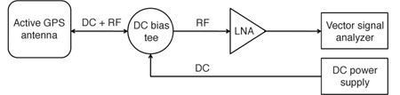
Method 1: Active Antenna Powered by GPS Receiver. The first method to power an active antenna is with a bias tee or DC power injector. Using this three-port component, a DC voltage (3.3 V in this case) is fed to its DC port, which applies the appropriate DC offset to the active antenna connected to the RF-in port while blocking it on the RF-out port. The device gets its name from the fact that the three ports are often arranged in the shape of a “T.” Note that the precise DC voltage one should apply depends on the DC power requirements of the active antenna. A diagram illustrating the connections is shown in Figure 3.
Observe in Figure 3 that one can use off-the-shelf hardware such as a programmable DC power supply to supply the DC bias signal. Also, one can use a generic off-the-shelf bias tee as long as it has bandwidth up to 1.58 GHz.
Figure 3. This set-up shows the use of a DC bias tee to power an active GPS antenna.
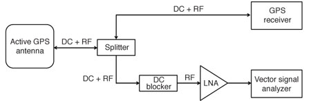
Method 2: Active GPS Antenna Powered by Receiver. A second method of powering the active GPS antenna is with the receiver itself. Most off-the-shelf GPS receivers use a single port to power and receive signals from an active GPS antenna, and this port is already biased with an appropriate DC voltage. Combining an active GPS receiver, a power splitter, and a DC blocker, one can power an active LNA and simply record essentially the same signal as that observed by the GPS receiver. A diagram of the appropriate connections is shown in Figure 4. Some splitters incorporate a DC block on all but one of the output ports.
As Figure 4 illustrates, the DC bias from the GPS receiver is used to power the LNA. This method is particularly useful for drive tests because one can observe the receiver’s characteristics, such as velocity and dilution of precision, while recording.
Figure 4. With a DC blocker, one can record and analyze the same GPS signals being tracked by a GPS receiver.
Selecting the Right LNA
Recording GPS signals with generic RF signal recorders is possible largely because external LNAs can be used to reduce the effective noise floor of the receiver. Today, one can find off-the-shelf spectrum analyzers with noise figures ranging from 15 dB to 20 dB. One of our analyzers, for example, has a 15 dB noise figure while applying up to 60 dB of gain. By applying external amplification to the front of an RF signal analyzer, however, one can substantially reduce the noise figure of the RF recording system.
To calculate the total noise that will be added to the recorded GPS signal, one must calculate the noise figure for the entire RF front end. As a matter of principle, the noise figure of the entire system is always dominated by the first amplifier in the system. Thus, careful selection of the first and second stage LNAs is crucial for a successful signal recording.
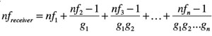
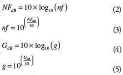
We can calculate the noise figure of the RF recording system by using the Friis formula for noise figure, named for engineer Harald Friis, a Danish-American radio engineer who worked at Bell Telephone Laboratories. To use this formula, first convert the gain and noise figure of each component to its linear equivalent; the latter is called the “noise factor.” For cascaded systems such as our RF recording system, the Friis formula provides us with the noise factor of the entire system:
(1)
Note that both noise factor (nf) and gain (g) are shown in lowercase to distinguish them as linear measures rather than logarithmic measures. The conversion from linear to logarithmic gain and noise figure (and vice v
ersa) is shown in the following equations:
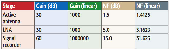
An active GPS antenna using a built-in LNA typically provides 30 dB of gain while introducing a noise figure that is typically on the order of 1.5 dB. The second part of the recording instrumentation provides 30 dB of additional gain as well. Though its noise figure is higher (5 dB), the second amplifier actually introduces very little noise into the system. As an academic exercise, one can use the Friis formula to calculate the noise factor for the entire RF front end of the recording instrumentation. Gain and noise figure values are shown in Table 1.
Table 1. Noise figures and factors of the first two components of the RF front end.
According to the calculations above, one can determine the overall noise factor for the receiver:
(6)
To convert noise factor into a noise figure (in dB), apply Equation 2, which yields the following results:
(7)
As Equation 7 illustrates, the noise figure of the first LNA (1.5 dB) dominates the noise figure of the entire RF recording system. Thus, with the VSA configured such that the noise floor of the instrument is less than that of the input stimulus, one’s recording introduces only 1.507 dB of noise to the off-the-air signal.
Saving Data to Disk
Each GNSS produces slightly varying requirements for an RF recorder’s signal bandwidth and center frequency. For the GPS C/A-codes, the essential requirement is to record 2.046 MHz of RF bandwidth at a center frequency of 1575.42 MHz.
In the tests described here, we set the IQ sample rate of our RF recorder at 5 megasamples per second (Ms/s). Since each 16-bit I and Q sample is 32 bits (or 4 bytes each), the actual recording data rate is 20 megabytes per second (MB/s) to ensure the entire bandwidth was captured. Capturing more than 4 MHz of bandwidth is sufficient to record the 2.046 MHz C/A-code signals.
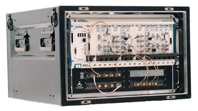
Because one can achieve data rates of 20 MB/s or more with standard PXI controller hard drives (PXI is the open, PC-based platform for test, measurement, and control), one does not need to use an external redundant array of independent disks (RAID) volume to stream GPS signals to disk when using a PXI recording system. In general, data rates exceeding 20 MB/s require the use of an external RAID volume. External RAID systems are capable of storing more than 600 MB/s of data and can be used to support wide bandwidth channels or even multi-channel recording applications. For example, the recording system shown in Figure 5 uses an external RAID volume for high-speed signal recording. This system combines PXI RF signal generators and analyzers with external amplifiers and filter banks for a ready-to-use GNSS record and playback solution.
Figure 5. Two-channel record and playback system from Averna.
In our tests, we decided to use a 320 GB USB drive for better portability. With a disk speed of 5400 revolutions per minute, we were able to benchmark it ahead of time and observed that we were able to achieve read and write speeds exceeding 25 MB/s. Thus, we were easily able to use this disk drive and still record IQ samples at 5 MS/s (20 MB/s) when recording off-the-air signals. With the existing hard-drive setup, we could record more than 4 hours of continuous IQ signal. Note that capturing longer recordings simply requires a larger hard disk. By using a 2 terabyte RAID volume (the largest addressable disk size in the Windows XP operating system), we can extend our recording time to 25 hours. With this setup, we could also reduce the IQ sample rate to 2.5 MS/s (still sufficient to capture the GPS C/A-code signals) and extend the recording time to 50 hours.
Receiver Performance
Once the off-the-air signal of a GNSS band is recorded to disk, it can be re-generated and fed to a receiver using an RF signal generator. With an RF signal generator that is able to reproduce the real-world GNSS signal, engineers are able to test a wide range of receiver characteristics. Because recorded signals contain a rich set of channel impairments such as ionosphere distortion and interference from other transmitters, design engineers often use recorded signals to prototype the baseband processing algorithms on a GNSS receiver.
In our case, we used a VSG directly connected to a GPS evaluation board. In the experiments described below, the receiver’s latitude, longitude, and velocity were tracked over time. Data was read from the receiver using a serial port, which read NMEA 0183 sentences at a rate of one per second. NMEA 0183 is a standard protocol developed by the National Marine Electronics Association for communications between marine electronic devices. NMEA 0183 has been adopted by virtually all GPS receiver manufacturers. In our LabVIEW graphical development environment, one can parse all sentences to return satellite and position-fix information.
For practical testing purposes, GPS dilution of precision and active satellites (GSA), GPS satellites in view (GSV), course over ground and ground speed (VTG), and GPS fix data (GGA) sentences are the most useful. More specifically, one can use information from the GSA sentence to determine whether the receiver has achieved a position fix and is used in time-to-first-fix measurements. When performing sensitivity measurements in this example, the GSV sentence was used to return carrier-to-noise-density ratios (C/N0) for each satellite being tracked. In addition, the VTG sentence allows us to observe the velocity of the receiver. Finally, the GGA sentence provides the receiver’s precise position by returning latitude and longitude information. See the references in Further Reading for in-depth information on the NMEA 0183 protocol.
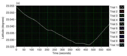
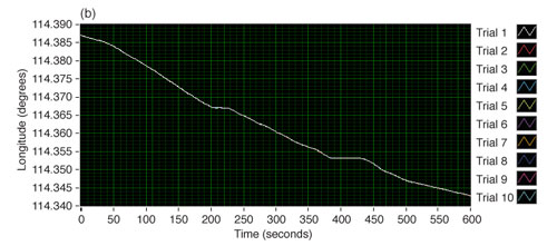
Using the receiver’s reported latitude and longitude information, we are able to test its ability to report a repeatable position when the recorded signal is played back to the receiver. In this experiment, we tracked the receiver position over 10 minutes. For the best results, the command interface of the receiver should be tightly synchronized with the start trigger of the RF signal generator. The results in Figure 6 show that the RF vector signal generator in this experiment was synchronized with the GPS receiver by using the data line of the serial communications (COM) port (RxD, pin 2) as a start trigger. Using this synchronization method, the vector signal generator and GPS receiver were synchronized to within one clock cycle of the VSG’s arbitrary waveform generator (100 MS/s). Thus, the maximum skew should be limited to 10 microseconds. Given our receiver’s maximum velocity of 15 meters per second (our maximum speed on the drive test), we can determine that the maximum error induced by clock offset of the signal generator is 10 microseconds x 15 meters per second, or 0.15 millimeters.
Using the configuration described above, one is able to report the receiver’s latitude and longitude over time, as shown in Figure 6.
Figure 6A. Receiver latitude over a four-minute span.Figure 6B. Receiver longitude over a four-minute span.
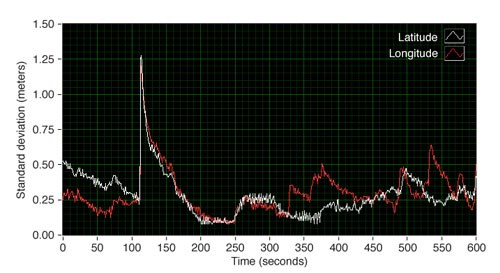
As the data from Figure 6 illustrate, a recorded test-drive signal reports static, position, and velocity information. In addition, one can observe that this information is relatively repeatable from one trial to the next, as evidenced by the difficulty in graphically observing each individual trace. To better characterize the deviation between each trace, one can also compute the standard deviation between each sample in the waveforms. Figure 7 illustrates the standard deviation between each of the 10 trials, calculated for every one-second interval, versus time.
Figure 7. Standard deviation of both latitude and longitude over time.
When observing the horizontal standard deviation, it is interesting to note that the standard deviation appears to rapidly increase at time = 120 seconds. To investigate this phenomenon further, we can plot the total horizontal standard deviation against the receiver’s velocity and a proxy for C/N0. In this case, we simply averaged the C/N0 values for the four highest satellites reported by the receiver. Since four satellites are required to achieve a three-dimensional position fix, our assumption was that position accuracy would closely correlate with the signal strength of these important satellite signals.
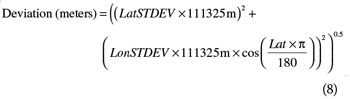
One simple method to evaluate the horizontal repeatability of the receiver position versus time is to calculate the standard deviation on a per-sample basis of each recorded latitude and longitude (in degrees). Once the standard deviation is measured in degrees, we can roughly convert this to meters with the following equation:
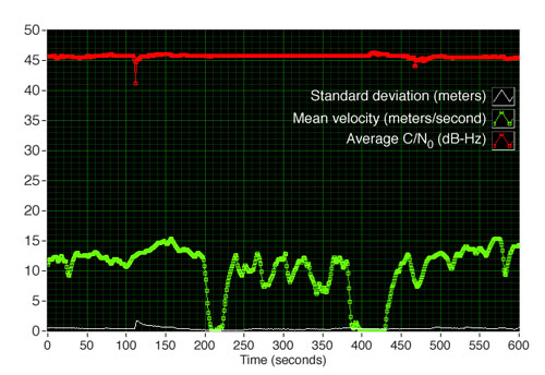
Note that Equation 8 represents a highly simplified error calculation method, which assumes that the Earth is a perfect sphere. For a more precise calculation of repeatability, the geodesic formula (which presumes that the Earth is ellipsoidal) should be used. In our simple experiment, the goal is merely to correlate repeatability with other factors that we can measure from the receiver. Figure 8 illustrates the standard deviation of horizontal position repeatability over 10 trials and at one-second time intervals.
Figure 8. Correlation of position accuracy and C/N0.
As one can observe in Figure 8, the peak horizontal error (measured by standard deviation) occurring at time = 120 seconds is directly correlated with satellite C/N0 and not correlated with receiver velocity. At this sample, the standard deviation is nearly 2 meters while it is less than 1 meter during most other times. Concurrently, the top four C/N0 averages drop from nearly 45 dB-Hz to 41 dB-Hz.
The exercise above illustrates not only the effect of C/N0 on position accuracy but also the types of analysis that one can conduct using recorded GPS data. For this experiment, the drive recording of the GPS signal was conducted in Huizhou, China (a city north of Shenzhen), but the actual receiver was tested at a later date in Austin, Texas.
Conclusion
In this article, we’ve illustrated how to use commercially available off-the-shelf products to record GPS signals with an RF recorder, and then play the signal back to a receiver. As the results illustrate, recorded GPS signals can be used to measure a wide range of receiver characteristics. Not only can receiver designers use these test techniques to better prototype a receiver baseband processor, but also to measure system-level performance such as position repeatability.
Manufacturers
The tests discussed in this article used a National Instruments PXIe-5663E, 6.6 GHz, RF signal analyzer; a National Instruments PXI-5690, 100 kHz to 3 GHz, two-channel programmable amplifier and attenuator; a National Instruments PXIe-5672, 2.7 GHz, RF vector signal generator with quadrature digital upconversion; a 320 GB USB Passport hard drive from Western Digital Corp.; a National Instruments PXI-4110 programmable, triple-output, precision DC power supply; and a ZX85-12G-S+ bias tee manufactured by Mini-Circuits. The article also mentioned the RP-3200 2-channel record and playback system manufactured by Averna, which incorporates National Instruments modules.
David Hall is an RF product manager for National Instruments. He holds a bachelor’s of science with honors in computer engineering from Pennsylvania State University.
FURTHER READING
More on GNSS Receiver Record and Playback Testing
GPS Receiver Testing, tutorial published by National Instruments, Austin, Texas.
Friis Formula and Receiver Performance
RF System Design of Transceivers for Wireless Communications by Q. Gu, published by Springer, New York, 2005.
Global Positioning System: Signals, Measurements, and Performance, 2nd edition, by P. Misra and P. Enge, published by Ganga-Jamuna Press, Lincoln, Massachusetts, 2006.
“Measuring GPS Receiver Performance: A New Approach” by S. Gourevitch in GPS World, Vol. 7, No. 10, October 1997, pp. 56-62.
“GPS Receiver System Noise” by R.B. Langley in GPS World, Vol. 8, No. 6, June 1997, pp. 40–45.
Global Positioning System: Theory and Applications, Vol. I, edited by B.W. Parkinson and J.J. Spliker Jr., published by the American Institute of Aeronautics and Astronautics, Inc., Washington, D.C., 1996.
GNSS Receiver Testing Using Simulators
“Testing Multi-GNSS Equipment: Systems, Simulators, and the Production Pyramid” by I. Petrovski, B. Townsend, and T. Ebinuma in Inside GNSS, Vol. 5, No. 5, July/August 2010, pp. 52–61.
“GPS Simulation” by M.B. May in GPS World, Vol. 5, No. 10, October 1994, pp. 51–56.
GNSS Receiver Testing Using Software
“GPS MATLAB Toolbox Review” by A.K. Tetewsky and A. Soltz in GPS World, Vol. 9, No. 10, October 1998, pp. 50–56.
GNSS L1 Signal Descriptions
Navstar GPS Space Segment / Navigation User Interfaces, Interface Specification, IS-GPS-200 Revision E, prepared by Science Applications International Corporation, El Segundo, California, for Global Positioning System Wing, June 2010.
Global Navigation Satellite System GLONASS, Interface Control Document, Navigational Radio Signal in Bands L1, L2 (Edition 5.1), prepared by Russian Institute of Space Device Engineering, Moscow, 2008.
NMEA 0183
NMEA 0183, The Standard for Interfacing Marine Electronic Devices, Ver. 4.00, published by the National Marine Electronics Association, Severna Park, Maryland, November 2008.
“NMEA 0183: A GPS Receiver Interface Standard” by R.B. Langley in GPS World, Vol. 6, No. 7, July 1995, pp. 54–57.
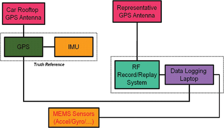
This article addresses how best to quantify “which navigation system performs best” in a realistic testing scenario. The methodology focuses on land vehicles navigating in urban environments, but applies equally well to pedestrian navigation and can be adapted for testing assisted-GNSS implementations. During a drive test, the truth-reference system and RF recording system log samples to disk, with no need for the receivers under test to be included during the actual drive.
By Eric Vinande, Brian Weinstein, Tianxing Chu, and Dennis Akos, University of Colorado, Boulder
FIGURE 1. Traditional in-vehicle receiver testing.
Radio frequency record-and-playback systems (RPS) have recently become commercially available. These systems sample the RF environment and store it to disk during a drive test and can replay it through receivers back in the lab environment. Here we explore the improvements in dynamic testing methodology created by these units.
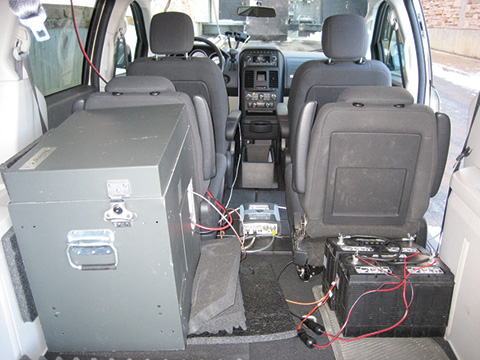
RPS test system installation.
RPS constitute a stark contrast to more traditional signal simulators that use pre-defined trajectories and mathematical models to determine appropriate RF output. Signal simulators attempt to reproduce environmental error factors such as multipath, inertial aiding system errors, and building and vehicle obstructions. They rely on mathematical models to simulate these various error sources. In some cases they do a reasonable job of reproducing these errors, but the dynamic urban environment is so complex (for example, rapidly varying/fading signal strength(s), multiple multipath signals, short/long duration obstructions of multiple layers) that even a sophisticated mathematical model can not replicate all effects completely. Some simulators include software that enables the user to define a trajectory and a limited amount of urban scenario details. Again, only so much realism can be created in a simulation environment. Existing testing standards are simulator-based, and as such, are circumscribed by the signal simulator limitations in representing a dynamic environment.
Positioning performance of a satellite navigation receiver under test (RUT) is coupled with its RF front-end system and local oscillator quality. Because of the variation in RF components between RUTs, some likely have superior RF interference (RFI) immunity. RFI can be a serious issue in certain land vehicles due to on-board electrical systems or because of external interference sources.
This article describes a testing method applicable to all receiver types, and complementary to that described in the December 2009 GPS World article by Mitelman and colleagues, “Testing Software Receivers,” regarding validation testing within a production environment. Added elements include taking into account truth-system uncertainty and a repeatability verification of the RF playback process through non-deterministic hardware receivers.
We present here the dynamic testing approach currently used at the University of Colorado in Boulder for receiver evaluation and comparison in the urban environment. The approach also includes the ability to assess the effect of sensor augmentations (for example, inertial, environmental) on positioning performance.
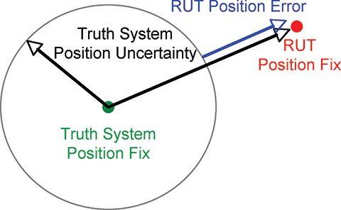
Truth Reference. Comparison with a truth reference system is essential for evaluation of satellite navigation receivers. For dynamic testing, this typically includes a survey-grade receiver coupled with a tactical-grade (or better) inertial measurement unit (IMU) and associated carrier-phase differential post-processing software. This software is filter-based and provides a positioning-error estimate in various components. Truth reference systems provide a continuous position estimate whose quality can vary depending on factors experienced in the urban environment, including length of full/partial satellite signal outage. In this study, we subtracted the 99th-percentile horizontal positioning error estimate of the truth system from the nominal RUT positioning error at each reporting epoch, as shown in Figure 2.
If the RUT position happens to lie within the truth-system position uncertainty, it is not considered to have any position error.
We focus here on a method to evaluate and compare mass-market, consumer-grade receivers to survey-grade receivers. One difference between these two receiver types is the way they handle the trade-off between accuracy and availability. Consumer receivers strive to provide the user with the highest availability, whereas survey receivers’ goal is to maximize accuracy. As a result, consumer-grade receivers will produce more regular position updates in harsh signal-tracking conditions, but must sacrifice accuracy to do so.
FIGURE 2. RUT position error calculation
Current Testing Standards
Currently accepted A-GPS standards such as those used by the 3rd Generation Partnership Project (3GPP) provide very limited dynamic testing in simulated urban conditions, being mainly designed to evaluate the first position calculation achieved in a particular simulated scenario. High-sensitivity receivers that pass or greatly exceed the 3GPP tests, in our opinion, are not guaranteed to have superior navigation performance in urban areas. Also, local oscillator performance is not specified. The trajectory dynamics imposed can actually be much smaller than the clock dynamics of a very low-cost local oscillator. A GPS receiver cannot tell the difference between the two and must track the effective Doppler variation.
The 3GPP defines five independent tests for A-GPS receiver certification. They include tests in the areas of: sensitivity with coarse/fine time assistance, nominal accuracy, dynamic range, multipath performance, and moving scenario/periodic update performance. The last three tests include elements that ostensibly pertain to the urban environment. These tests specify discrete, constant signal power levels for implementation in a hardware signal simulator. The discrepancy between the 3GPP-prescribed signal levels and those observed during actual drive testing is detailed as follows.
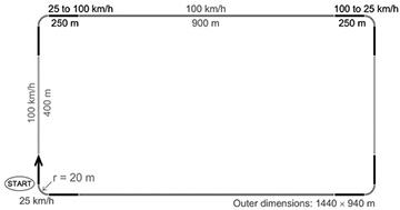
The 3GPP moving scenario/periodic update performance test trajectory is shown in Figure 3.
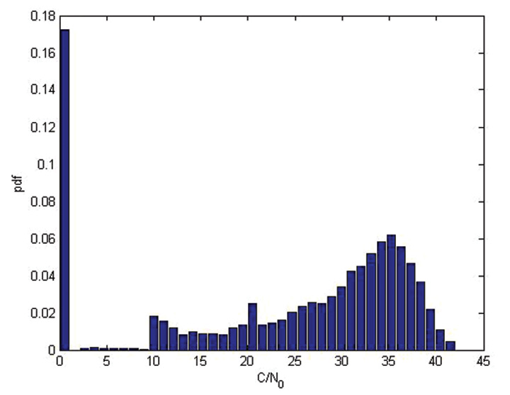
This test profile calls for the simulation of five satellites with a constant signal strength of 2130 dBm while the vehicle travels around the racetrack trajectory. In contrast, during an actual drive test in an urban area, a receiver reported the distribution of carrier-to-noise-density values for all tracked satellites as shown in Figure 4. This more accurately shows the range of signal strengths that should be expected in urban conditions.
FIGURE 4. Drive-test C/N0 distribution
The 3GPP moving test is considered passed if positions are reported regularly, and 95 percent of them are within 100 meters of the true position. This is not a particularly difficult test for a RUT to retain signal lock through, as the linear acceleration is about 0.15 g and the centripetal acceleration is about 0.25 g.
It is difficult for independent third parties to carry out a receiver evaluation following 3GPP guidelines as several of the tests require receiver restarts, which in turn requires testing automation. Depending on the receiver-evaluation hardware availability, restart commands may not be available to to an independent evaluator.
3GPP receiver testing results are quoted as pass or fail over a large number of short evaluations. For the dynamic environment, the system performance over continuous time is required to make a proper comparison between evaluated receivers.
In general, evaluating the GPS engines embedded within cell phones or other devices is difficult. Most are not made to interface with an external antenna, and the mere act of adding an antenna connection can significantly alter performance. The output format is not always documented, if it is even available to an end user. To allow fair across-the-board comparisons, GPS chipset manufacturers should make available development kits that have external antenna connections and well-documented message output formats.
Drive-Test Configuration
Current live dynamic testing requires multiple systems to be operating in a moving vehicle (see opening Figure 1). A truth-reference system, usually a high-grade GPS/INS device along with post-processing, provides the basis to which all other RUT are compared. This system requires a dedicated vehicle rooftop antenna with the best possible sky view, separate from a lower-grade test antenna located within the vehicle. Each RUT is connected to the representative consumer-grade antenna located in the vehicle through a high-isolation splitter that suppresses inter-receiver interference. It is important at this point that the gain be set appropriately for each RUT, depending on the front-end expectations while maintaining an equivalent noise figure across all receivers.
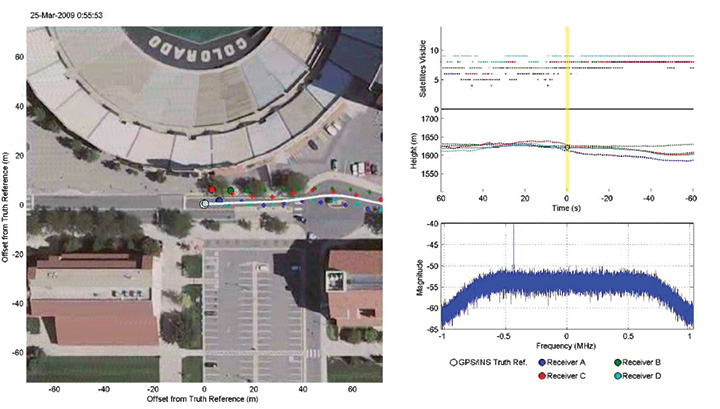
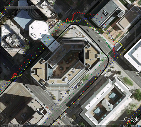
Visualization Methods
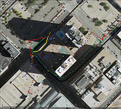
In addition to quantitative methods, we have created a qualitative visualization to assist with interpretation of the raw data. The same parsed data sets that provide the statistical script input are fed into a viewer script along with the post-processed truth reference data. With the truth-reference system data plotted in the center of the screen, each RUT is then plotted the correct distance and direction away, based on the distance and direction of error compared to truth. The receiver plots are overlaid onto Google Earth images centered on the truth-reference location. Plots of number of satellites utilized (top right of Figure 5) and elevation (middle right) as reported by each receiver and the sampled RF spectrum (lower right) are also included.
For each reporting epoch, based on the data frequency of the truth-reference system, a frame is generated with the aforementioned characteristics. These frames are gathered and encoded into a movie clip which can then be used as a quick and simple qualitative tool for receiver comparison. Figure 5 shows an individual movie frame. A forward-looking camera capability is also being added to this movie so the test environment can be documented from multiple angles.
FIGURE 5. Movie visualization screenshot
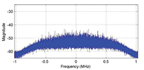
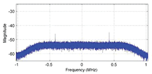
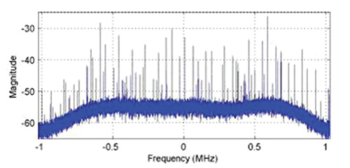
While observing this movie, variations in the sampled RF spectrum from interference or blockages can be associated with the current landscape. Locations of RFI sources can be identified and avoided (or included) in future testing. These RFI and significant blockage locations are of interest for receiver RF component and navigation filter development. The next three figures show spectrum snapshots during various parts of a drive test. In Figure 6, the cumulative GPS spectra rises above the noise floor and is visible during open sky conditions. While below ground level, Figure 7 shows only the front-end filter shape (and relatively minor RFI). Figure 8 shows an example of severe RFI when near a specific parking garage location.
FIGURE 6. Open-sky spectrum (centered on 1575.42 MHz)
FIGURE 7. Spectrum while below ground level (centered on 1575.42 MHz).
FIGURE 8. Spectrum near interference source (centered on 1575.42 MHz).
Record/Playback Concept
To overcome the limitations of hardware signal simulators and repeated vehicle drive testing, the RF record/playback testing method is utilized at the university. Commercially available equipment, capable of recording and playing back an RF signal, has recently become available. Equipment options exist for between $10,000–100,000, with 1–16 bit sampling and 4–25 MHz front-end bandwidth.
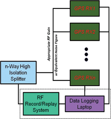
Figures 9 and 10 show the concept of “record once, playback many times.” During a drive test, the truth-reference system and RF recording system log samples to disk. There is no need for the RUT to be included during the actual drive test.
In the laboratory, the logged RF samples are replayed through a splitter to all RUT. The effect of receiver configuration changes can be evaluated without having to repeat the drive test. At a later time, additional receivers can also be tested using the same stored RF sample file.
During separate record and playback phases, testing considerations and methods discussed previously are implemented.
Since the recording process can only obviously capture current conditions, additional drive-test collections are required if different satellite geometry is desired, or if additional representative antennas need to be evaluated.
Repeatability of RPS Testing
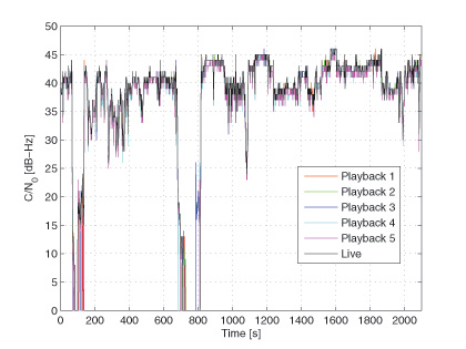
To validate that the playback signal levels were not significantly different from live signals, we conducted an urban, dynamic evaluation. Figure 11 shows that there is typically not more than a 1 dB difference in reported C/N0 between live and playback modes when testing a receiver that only reported integer values. The two dropout instances were excursions into parking garages.
FIGURE 11. Live and playback C/N0 values
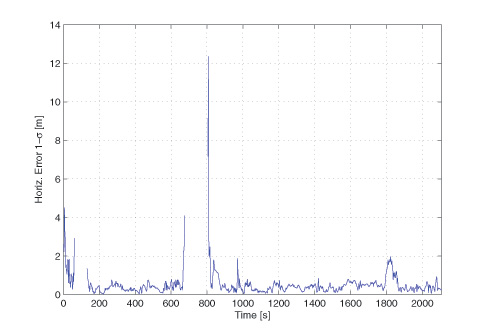
Figure 12 compares the navigation statistics between replays, using the same five playbacks as in Figure 11. The playbacks show a 1-sigma horizontal position solution spread under 1 meter for approximately 83 percent of the test.
FIGURE 12. Playback Horizontal Position Error Spread.
These two figures verify the repeatability of the RPS testing method and solidify it as an alternative to both signal-simulator testing and live testing of satellite navigation receivers.
Denver Testing Method
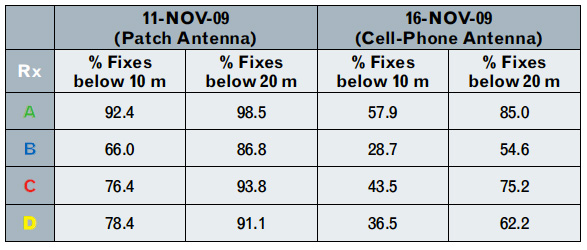
To evaluate the RPS concept, we conducted tests in three locations: Boulder, Denver, and Interstate Highway 70, all in Colorado. The Boulder and Denver locations were urban collections, while the Interstate 70 location was a natural canyon with significant elevation change. The collection at each location was repeated with two different representative antennas (patch and cell phone) at nearly the same sidereal time in order to keep the overhead satellite constellation similar.
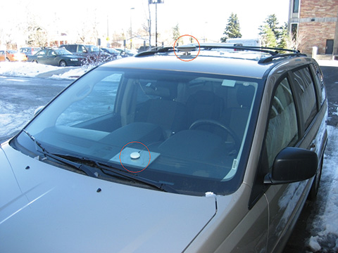
We examine here the November 11 and 16 Denver tests. The November 11 test used a patch antenna that places nearly all its gain in the upward direction, making it more immune to interfering sources below and to its sides. Figure 13 shows the patch antenn
a location on the van, as well as the truth-system antenna location utilized for testing on both days.
FIGURE 13. Patch antenna (dashboard) and truth-system antenna (rooftop) locations.
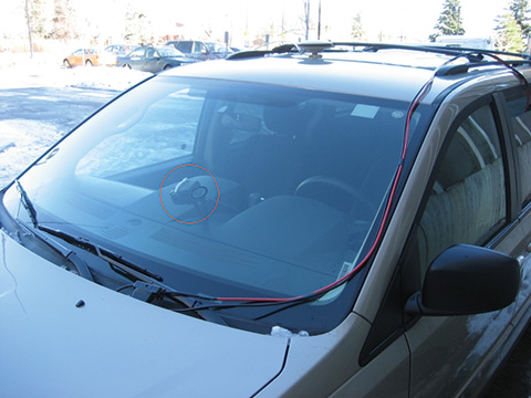
The November 16 test used a cell-phone GPS antenna that does not have a preferential gain direction, making it more susceptible to interfering sources below and to its sides. This antenna type is representative of the typical low-cost antenna (in some cases as simple as a piece of wire) found in consumer cell phones. Figure 14 shows the cell-phone antenna suction-cup mounted to the front window of the testing van. The representative antenna mounting location was chosen to minimize locally-generated RFI effects while also being representative of a typical vehicle-use case.
FIGURE 14. Cell-phone antenna location.
The required equipment and connections are minimal when performing RPS drive testing, as no RUTs are included. The inset to Figure 1 at the beginning of this article shows the RPS unit in the rear of the van, mounted on layers of foam to reduce vibration, which, if not properly addressed, can cause errors in mechanical hard drives writing data at high rates. Also visible are the truth receiver on the center of the van floor, and the car batteries for powering it and the IMU. The IMU is mounted to the vehicle frame and is not shown.
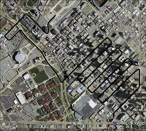
The test drive trajectory through Denver on November 11 and 16 as reported by the truth system is shown in black in Figure 15 and is also repeated in Figures 16 and 17. The test lasted approximately 40 minutes on both days. It started in the upper left part of Figure 15 and continued zig-zagging through downtown to the lower right.
FIGURE 15. Truth trajectory for November 11 and 16 tests.
Figures 16 and 17 show particularly difficult blocks for the four receivers tested under the replay method. These receivers are denoted A (green), B (blue), C (red), and D (yellow).
FIGURE 16. Difficult block #1 during November 11 test and truth system antenna (rooftop) locations.
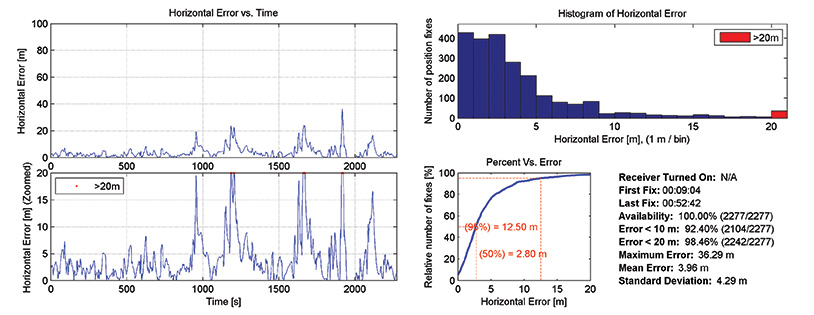
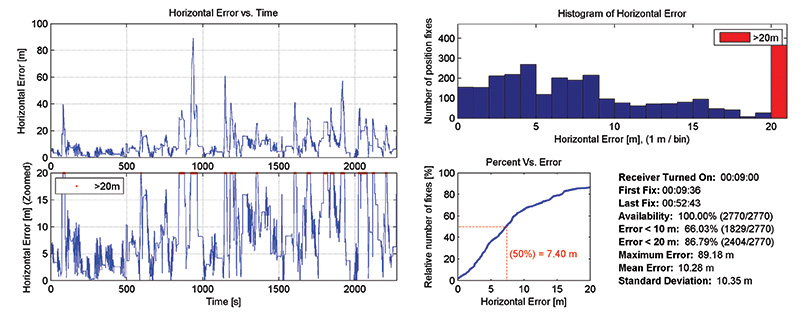
The horizontal positioning error statistics for two receivers on the November 11 test are shown in Figures 18 and 19. The left side shows horizontal error in two different zoom levels. The right side shows a histogram and cumulative distribution of errors, and several reporting metrics over the entire test. Even though receiver A in general outperformed receiver B, from the error time histories there are noticeable periods where both receivers simultaneously had positioning difficulties.
FIGURE 17. Difficult block #2 during November 11 test.
Table 1 summarizes the horizontal positioning statistics for all receivers during both tests. Positioning accuracy was severely degraded when replaying samples collected with the cell-phone antenna as compared to the patch antenna. Receiver A was the most accurate across both tests, while receiver B was the least accurate. The uncertainty of the truth system was subtracted out when producing the horizontal positioning results for all receivers.
Table 1
Conclusions
The record-and-playback system testing approach, in our opinion, represents the best way to test hardware receivers. It overcomes the fidelity limits of simulator-based testing, especially when considering the difficult-to-model urban environment. During receiver development, it requires only a single drive test for each location, as sampled RF data can be replayed from disk.
Having demonstrated that RPS testing is repeatable, we have produced a library of RF sample files representing real-world conditions for continued receiver development and testing purposes.
Eric Vinande is Ph.D. student at the University of Colorado studying GPS/MEMS inertial sensor integration and urban RFI aspects.
Brian Weinstein is a BSEE student participating in the Undergraduate Research Opportunity Program for GNSS receiver testing at the University of Colorado.
Tianxing Chu is a visiting researcher at the University of Colorado from Peking University where he is a Ph.D. student.
Dennis Akos is an associate professor within the Aerospace Engineering Sciences Department at the University of Colorado with concurrent appointments at Stanford University and Luleå University of Technology.
Manufacturers
Development of the methodology described here used two different RPS systems, one from LabSat (RaceLogic) and one from Averna. The test data come from the Averna system.
Navigation and positioning test system supplier Spirent Communications this week introduced a software suite for the STR4500 GPS simulator, enabling users to generate their own test cases based on motion data that fits their specific requirements, the company said.
Launched in 2001, the STR4500 provides pre-defined test cases for the testing of GPS receivers and systems to be replayed using a PC-based controller with RF signal generator hardware. Typical users of the STR4500 are involved with the selection, integration, verification or production test of GPS L1 C/A code systems, according to Spirent.
The new SimPLEX45 software enables unique test cases to be generated, saved and run directly by the user. SimPLEX45 also enables user-defined motion-data to be used with atmospheric models and the environment around a vehicle, the company said.
“This new software will enable our customers to drive a route and, using logged NMEA data, generate a trajectory for a test case,” stated John Pottle, marketing director for Spirent’s Wireless and Positioning Division. “The user also will be able to define the antenna pattern, atmospheric effect and obscuration due to buildings or other obstructions. We’ve built this capability into the STR4500 to provide our customers with reduced development times via improved tailoring of test scenarios to fit their specific needs.”
The SimPLEX45 is available with new systems or as an easy to install upgrade to existing STR4500 users, Spirent said.
To initially acquire the GPS signals, a receiver also would have to search quickly through the much larger range of possible Doppler shifts and code delays than those experienced by a terrestrial receiver.
By William Bamford, Luke Winternitz and Curtis Hay
INNOVATION INSIGHTS by Richard Langley
GPS RECEIVERS have been used in space to position and navigate satellites and rockets for more than 20 years. They have also been used to supply accurate time to satellite payloads, to determine the attitude of satellites, and to profile the Earth’s atmosphere. And GPS can be used to position groups of satellites flying in formation to provide high-resolution ground images as well as small-scale spatial variations in atmospheric properties and gravity.
Receivers in low Earth orbit have virtually the same view of the GPS satellite constellation as receivers on the ground. But satellites orbiting at geostationary altitudes and higher have a severely limited view of the main beams of the GPS satellites. The main beams are either directed away from these high-altitude satellites or they are blocked to a large extent by the Earth.
Typically, not even four satellites can be seen by a conventional receiver. However, by using the much weaker signals emitted by the GPS satellite antenna side lobes, a receiver may be able track a sufficient number of satellites to position and navigate itself. To initially acquire the GPS signals, a receiver also would have to search quickly through the much larger range of possible Doppler shifts and code delays than those experienced by a terrestrial receiver.
In this month’s column, William Bamford, Luke Winternitz, and Curtis Hay discuss the architecture of a receiver with these needed capabilities — a receiver specially designed to function in high Earth orbit. They also describe a series of tests performed with a GPS signal simulator to validate the performance of the receiver here on the ground — well before it debuts in orbit.
“Innovation” is a regular column featuring discussions about recent advances in GPS technology and its applications as well as the fundamentals of GPS positioning. The column is coordinated by Richard Langley of the Department of Geodesy and Geomatics Engineering at the University of New Brunswick, who appreciates receiving your comments and topic suggestions. To contact him, see the “Columnists” section in this issue.
Calculating a spacecraft’s precise location at high orbits — 22,000 miles (35,400 kilometers) and beyond — is an important and challenging problem. New and exciting opportunities become possible if satellites are able to autonomously determine their own orbits.
First, the repetitive task of periodically collecting range measurements from terrestrial antennas to high-altitude spacecraft becomes less important — this lessens competition for control facilities and saves money by reducing operational costs. Also, autonomous navigation at high orbital altitudes introduces the possibility of autonomous station-keeping. For example, if a geostationary satellite begins to drift outside of its designated slot, it can make orbit adjustments without requiring commands from the ground. Finally, precise onboard orbit determination opens the door to satellites flying in formation — an emerging concept for many scientific space applications.
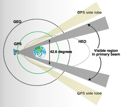
Realizing these benefits is not a trivial task. While the navigation signals broadcast by GPS satellites are well suited for orbit and attitude determination at lower altitudes, acquiring and using these signals at geostationary (GEO) and highly elliptical orbits (HEOs) is much more difficult. This situation is illustrated in FIGURE 1.
Figure 1. GPS signal reception at GEO and HEO orbital altitudes.
The light blue trace shows the GPS orbit at approximately 12,550 miles (20,200 kilometers) altitude. GPS satellites were designed to provide navigation signals to terrestrial users — because of this, the antenna array points directly toward the Earth. GEO and HEO orbits, however, are well above the operational GPS constellation, making signal reception at these altitudes more challenging. The nominal beamwidth of a Block II/IIA GPS satellite antenna array is approximately 42.6 degrees. At GEO and HEO altitudes, the Earth blocks most of these primary beam transmissions, leaving only a narrow region of nominal signal visibility near the limb of the Earth.This region is highlighted in gray.
If GPS receivers at GEO and HEO orbits were designed to use these higher power signals only, precise orbit determination would not be practical. Fortunately, the GPS satellite antenna array also produces side-lobe signals at much lower power levels. The National Aeronautics and Space Administration (NASA) has designed and tested the Navigator, a new GPS receiver that can acquire and track these weaker signals, dramatically increasing signal visibility at these altitudes.
While using much weaker signals is a fundamental requirement for a high orbital altitude GPS receiver, it is certainly not the only challenge. Other unique characteristics of this application must also be considered. For example, position dilution of precision (PDOP) figures are much higher at GEO and HEO altitudes because visible GPS satellites are concentrated in a much smaller region with respect to the spacecraft antenna. These poor PDOP values contribute considerable error to the point-position solutions calculated by the spacecraft GPS receiver.
Extreme Conditions. Finally, spacecraft GPS receivers must be designed to withstand a variety of extreme environmental conditions. Variations in acceleration between launch and booster separation are extreme. Temperature gradients in the space environment are also severe. Furthermore, radiation effects are a major concern — spaceborne GPS receivers should be designed with radiation-hardened parts to minimize damage caused by continuous exposure to low-energy radiation as well as damage and operational upsets from high-energy particles. Perhaps most importantly, we typically cannot repair or modify a spaceborne GPS receiver after launch. Great care must be taken to ensure all performance characteristics are analyzed before liftoff.
Motivation
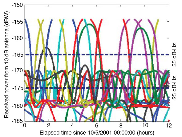
As mentioned earlier, for a GPS receiver to autonomously navigate at altitudes above the GPS constellation, its acquisition algorithm must be sensitive enough to pick up signals far below that of the standard space receiver. This concept is illustrated in FIGURE 2. The colored traces represent individual GPS satellite signals. The topmost dotted line represents the typical threshold of traditional receivers. It is evident that such a receiver would only be able to track a couple of the strong, main-lobe signals at any given time, and would have outages that can span several hours.
The lower dashed line represents the design sensitivity of the Navigator receiver. The 10 dB reduction allows Navigator to acquire and track the much weaker side-lobe signals. These side lobes augment the main lobes when available, and almost completely eliminate any GPS signal outages. This improved sensitivity is made possible by the specialized acquisition engine built into Navigator’s hardware.
Figure 2. Simulated received power at GEO orbital altitude.
Acquisition Engine
Signal acquisition is the first, and possibly most difficult, step in the GPS signal processing procedure. The acquisition task requires a search across a three-dimensional parameter space that spans the unknown time delay, Doppler shift, and the GPS satellite pseudorandom noise codes. In space applications, this search space can be extremely large, unless knowledge of the receiver’s position, velocity, current time, and the location of the desired GPS satellite are available beforehand.
Serial Search. The standard approach to this problem is to partition the unknown Doppler-delay space into a sufficiently fine grid and perform a brute force search over all possible grid points. Traditional receivers use a handful of tracking correlators to serially perform this search. Without sufficient information up front, this process can take 10–20 minutes in a low Earth orbit (LEO), or even terrestrial applications, and much longer in high-altitude space applications. This delay is due to the exceptionally large search space the receiver must hunt through and the inefficiency of serial search techniques.
Acquisition speed is relevant to the weak signal GPS problem, because acquiring weak signals requires the processing of long data records. As it turns out, using serial search methods (without prior knowledge) for weak signal acquisition results in prohibitively long acquisition times.
Many newer receivers have added specialized fast-acquisition capability. Some employ a large array of parallel correlators; others use a 32- to 128-point fast Fourier transform (FFT) method to efficiently resolve the frequency dimension. These methods can significantly reduce acquisition time. Another use of the FFT in GPS acquisition can be seen in FFT-correlator-based block-processing methods, which offer dramatically increased acquisition performance by searching the entire time-delay dimension at once. These methods are popular in software receivers, but because of their complexity, are not generally used in hardware receivers.
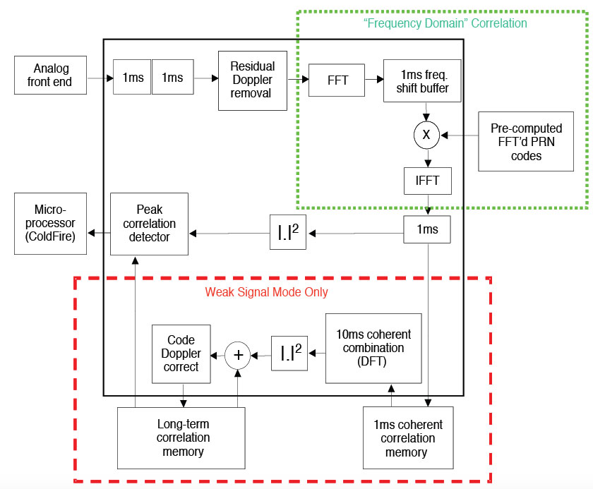
Exceptional Navigator. One exception is the Navigator receiver. It uses a highly specialized hardware acquisition engine designed around an FFT correlator. This engine can be thought of as more than 300,000 correlators working in parallel to search the entire Doppler-delay space for any given satellite. The module operates in two distinct modes: strong signal mode and weak signal mode. Strong signal mode processes a 1 millisecond data record and can acquire all signals above –160 dBW in just a few seconds. Weak signal mode has the ability to process arbitrarily long data records to acquire signals down to and below –175 dBW. At this level, 0.3 seconds of data are sufficient to reliably acquire a signal.
Additionally, because the strong, main-lobe, signals do not require the same sensitivity as the side-lobe signals, Navigator can vary the length of the data records, adjusting its sensitivity on the fly. Using essentially standard phase-lock-loop/delay-lock-loop tracking methods, Navigator is able to track signals down to approximately –175 dBW. When this tracking loop is combined with the acquisition engine, the result is the desired 10 dB sensitivity improvement over traditional receivers. FIGURE 3 illustrates Navigator’s acquisition engine.
Powered by this design, Navigator is able to rapidly acquire all GPS satellites in view, even with no prior information. In low Earth orbit, Navigator typically acquires all in-view satellites within one second, and has a position solution as soon as it has finished decoding the ephemeris from the incoming signal. In a GEO orbit, acquisition time is still typically under a minute.
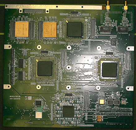
Figure 3. Navigator signal acquisition engine.Navigator breadboard.GPS constellation simulator.
Navigator Hardware
Outside this unique acquisition module, Navigator employs the traditional receiver architecture: a bank of hardware tracking correlators attached to an embedded microprocessor. Navigator’s GPS signal-processing hardware, including both the tracking correlators and the acquisition module, is implemented in radiation-hardened field programmable gate arrays (FPGAs). The use of FPGAs, rather than an application-specific integrated circuit, allows for rapid customization for the unique requirements of upcoming missions. For example, when the L2 civil signal is implemented in Navigator, it will only require an FPGA code change, not a board redesign.
The current Navigator breadboard—which, during operation, is mounted to a NASA-developed CPU card—is shown in the accompanying photo. The flight version employs a single card design and, as of the writing of this article, is in the board-layout phase. Flight-ready cards will be delivered in October 2006.
Integrated Navigation Filter
Even with its acquisition engine and increased sensitivity, Navigator isn’t always able to acquire the four satellites needed for a point solution at GEO altitudes and above. To overcome this, the GPS Enhanced Onboard Navigation System (GEONS) has been integrated into the receiver software. GEONS is a powerful extended Kalman filter with a small package size, ideal for flight-software integration. This filter makes use of its internal orbital dynamics model in conjunction with incoming measurements to generate a smooth solution, even if fewer than four GPS satellites are in view.
The GEONS filter combines its high-fidelity orbital dynamics model with the incoming measurements to produce a smoother solution than the standard GPS point solution. Also, GEONS is able to generate state estimates with any number of visible satellites, and can provide state estimation even during complete GPS coverage outages.
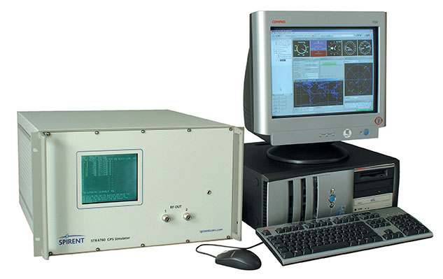
Hardware Test Setup
We used an external, high-fidelity orbit propagator to generate a two-day GEO trajectory, which we then used as input for the Spirent STR4760 GPS simulator. This equipment, shown in the accompanying photo, combines the receiver’s true state with its current knowledge of the simulated GPS constellation to generate the appropriate radio frequency (RF) signals as they would appear to the receiver’s antenna. Since there is no physical antenna, the Spirent SimGEN software package provides the capability to model one.
The Navigator receiver begins from a cold start, with no advance knowledge of its position, the position of the GPS satellites, or the current time. Despite this lack of information, Navigator typically acquires its first satellites within a minute, and often has its first position solution within a few minutes, depending on the number of GPS satellites in view. Once a position solution has been generated, the receiver initializes the GEONS navigation filter and provides it with measurements on a regular, user-defined basis. The Navigator point solution is output through a high-speed data acquisition card, and the GEONS state estimates, covariance, and measurement residuals are exported through a serial connection for use in data analysis and post-processing.
We configured the GPS simulator to model the receiving antenna as a hemispherical antenna with a 135-degree field-of-view and 4 dB of received gain, though this antenna would not be optimal for the GEO case. Assuming a nadir-pointing antenna, all GPS signals are received within a 40-degree angle with respect to the bore sight. Furthermore, no signals arrive from between 0 and 23 degrees elevation angle because the Earth obstructs this range. An optimal GEO antenna (possibly a high-gain array) would push all of the gain into the feasible elevation angles for signal reception, which would greatly improve signal visibility for Navigator (a traditional receiver would still not see the side lobes). Nonetheless, the following results provide an important baseline and demonstrate that a high-gain antenna, which would increase size and cost of the receiver, may not be necessary with Navigator. The GPS satellite transmitter gain patterns were set to model the Block II/IIA L1 reference gain pattern.
Simulation Results
To validate the receiver designs, we ran several tests using the configuration described above. The following section describes the results from a subset of these tests.
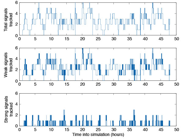
Tracked Satellites. The top plot of FIGURE 4 illustrates the total number of satellites tracked by the Navigator receiver during a two-day run with the hemispherical antenna. On average, Navigator tracked between three and four satellites over the simulation period, but at times as many as six and as few as zero were tracked. The middle pane depicts the number of weak signals tracked—signals with received carrier-to-noise-density ratio of 30 dB-Hz or less. The bottom panel shows how many satellites a typical space receiver would pick up. It is evident that Navigator can track two to three times as many satellites at GEO as a typical receiver, but that most of these signals are weak.
Figure 4. Number of satellites tracked in GEO simulation.
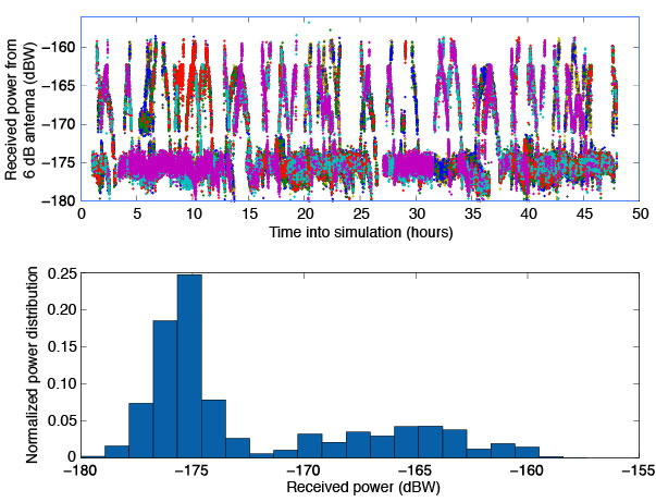
Acquisition Thresholds. The received power of the signals tracked with the hemispherical antenna is plotted in the top half of FIGURE 5. The lowest power level recorded was approximately –178 dBW, 3 dBW below the design goal. (Note the difference in scale from Figure 1, which assumed an additional 6 dB of antenna gain.) The bottom half of Figure 5 shows a histogram of the tracked signals. It is clear that most of the signals tracked by Navigator had received power levels around –175 dBW, or 10 dBW weaker than a traditional receiver’s acquisition threshold.
Figure 5. Signal tracking data from GEO simulation.
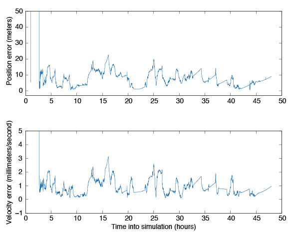
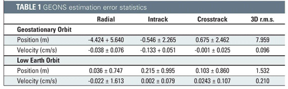
Navigation Filter. To validate the integration of the GEONS software, we compared its estimated states to the true states over the two-day period. These results are plotted in FIGURE 6. For this simulation, we assumed that GPS satellite clock and ephemeris errors could be corrected by applying NASA’s Global Differential GPS System corrections, and errors caused by the ionosphere could be removed by masking signals that passed close to the Earth’s limb. The truth environment consisted of a 70X70 degree-and-order gravity model and sun-and-moon gravitational effects, as well as drag and solar-radiation pressure forces. GEONS internally modeled a 10X10 gravity field, solar and lunar gravitational forces, and estimated corrections to drag and solar-radiation pressure parameters. (Note that drag is not a significant error source at these altitudes.) Though the receiver produces pseudorange, carrier-phase, and Doppler measurements, only the pseudorange measurement is being processed in GEONS.
Figure 6. GEONS state estimation errors for GEO simulation.
The results, compiled in TABLE 1, show that the 3D root mean square (r.m.s.) of the position error was less than 10 meters after the filter converges. The velocity estimation agreed very well with the truth, exhibiting less than 1 millimeter per second of three-dimensional error. Navigator can provide excellent GPS navigation data at low Earth orbit as well, with the added benefit of near instantaneous cold-start signal acquisition. For completeness, the low Earth orbit results are included in Table 1.
Navigator’s Future
Navigator’s unique features have attracted the attention of several NASA projects. In 2007, Navigator is scheduled to launch onboard the Space Shuttle as part of the Hubble Space Telescope Servicing Mission 4: Relative Navigation Sensor (RNS) experiment. Additionally, the Navigator/GEONS technology is being considered as a critical navigational instrument on the new Geostationary Operational Environmental Satellites (GOES-R).
In another project, the Navigator receiver is being mated with the Intersatellite Ranging and Alarm System (IRAS) as a candidate absolute/relative state sensor for the Magnetospheric Multi-Scale Mission (MMS). This mission will transition between several high-altitude highly elliptical orbits that stretch well beyond GEO. Initial investigations and simulations using the Spirent simulator have shown that Navigator/GEONS can easily meet the mission’s positioning requirements, where other receivers would certainly fail.
Conclusion
NASA’s Goddard Space Flight Center has conducted extensive test and evaluation of the Navigator GPS receiver and GEONS orbit determination filter. Test results, including data from RF signal simulation, indicate the receiver has been designed properly to autonomously calculate precise orbital information at altitudes of GEO and beyond. This is a remarkable accomplishment, given the weak GPS satellite signals observed at these altitudes. The GEONS filter is able to use the measurements provided by the Navigator receiver to calculate precise orbits to within 10 meters 3D r.m.s. Actual flight test data from future missions including the Space Shuttle RNS experiment will provide further performance characteristics of this equipment, from which its suitability for higher orbit missions such as GOES-R and MMS can be confirmed.
Manufacturers
The Navigator receiver was designed by the NASA Goddard Space Flight Center Components and Hardware Systems Branch (Code 596) with support from various contractors. The 12-channel STR4760 RF GPS signal simulator was manufactured by Spirent Communications (www.spirentcom.com).
FURTHER READING
1. Navigator GPS receiver
“Navigator GPS Receiver for Fast Acquisition and Weak Signal Tracking Space Applications” by L. Winternitz, M. Moreau, G. Boegner, and S. Sirotzky, in Proceedings of ION GNSS 2004, the 17th International Technical Meeting of the Satellite Division of The Institute of Navigation, Long Beach, California, September 21–24, 2004, pp. 1013-1026.
“Real-Time Geostationary Orbit Determination Using the Navigator GPS Receiver” by W. Bamford, L. Winternitz, and M. Moreau in Proceedings of NASA 2005 Flight Mechanics Symposium, Greenbelt, Maryland, October 18–20, 2005 (in press). A pre-publication version of the paper is available online at http://www.emergentspace.com/pubs/Final_GEO_copy.pdf.
1. GPS on high-altitude spacecraft
“The View from Above: GPS on High Altitude Spacecraft” by T.D. Powell in GPS World, Vol. 10, No. 10, October 1999, pp. 54–64.
“Autonomous Navigation Improvements for High-Earth Orbiters Using GPS” by A. Long, D. Kelbel, T. Lee, J. Garrison, and J.R. Carpenter, paper no. MS00/13 in Proceedings of the 15th International Symposium on Spaceflight Dynamics, Toulouse, June 26–30, 2000. Available online at http://geons.gsfc.nasa.giv/library_docs/ISSFDHEO2.pdf.
1. GPS for spacecraft formation flying
“Autonomous Relative Navigation for Formation-Flying Satellites Using GPS” by C. Gramling, J.R. Carpenter, A. Long, D. Kelbel, and T. Lee, paper MS00/18 in Proceedings of the 15th International Symposium on Spaceflight Dynamics, Toulouse, June 26–30, 2000. Available online at http://geons.gsfc.nasa.giv/library_docs/ISSFDrelnavfinal.pdf.
“Formation Flight in Space: Distributed Spacecraft Systems Develop New GPS Capabilities” by J. Leitner, F. Bauer, D. Folta, M. Moreau, R. Carpenter, and J. How in GPS World, Vol. 13, No. 2, February 2002, pp. 22–31.
1. Fourier transform techniques in GPS receiver design
“Block Acquisition of Weak GPS Signals in a Software Receiver” by M.L. Psiaki in Proceedings of ION GPS 2001, the 14th International Technical Meeting of the Satellite Division of The Institute of Navigation, Salt Lake City, Utah, September 11–14, 2001, pp. 2838–2850.
1. Testing GPS receivers before flight
“Pre-Flight Testing of Spaceborne GPS Receivers Using a GPS Constellation Simulator” by S. Kizhner, E. Davis, and R. Alonso in Proceedings of ION GPS-99, the 12th International Technical Meeting of the Satellite Division of The Institute of Navigation, Nashville, Tennessee, September 14–17, 1999, pp. 2313–2323.
BILL BAMFORD is an aerospace engineer for Emergent Space Technology, Inc., in Greenbelt, Maryland. He earned a Ph.D. from the University of Texas at Austin in 2004, where he worked on precise formation flying using GPS as the primary navigation sensor. As an Emergent employee, he has worked on the development of the Navigator receiver and helped support and advance the NASA Goddard Space Flight Center’s Formation Flying Testbed. He can be reached at [email protected].
LUKE WINTERNITZ is an electrical engineer in hardware components and systems at NASA’s Goddard Space Flight Center in Greenbelt, Maryland. He has worked at Goddard for three years primarily in the development of GPS receiver technology. He received bachelor’s degrees in electrical engineering and mathematics from the University of Maryland, College Park, in 2001 and is a part-time graduate student there pursuing a Ph.D. He can be reached at [email protected].
CURTIS HAY served as an officer in the United States Air Force for eight years in a variety of GPS-related assignments. He conducted antijam GPS R&D for precision weapons and managed the GPS Accuracy Improvement Initiative for the control segment. After separating from active duty, he served as the lead GPS systems engineer for OnStar. He is now a systems engineer for Spirent Federal Systems in Yorba Linda, California, a supplier of high-performance GPS test equipment. He can be reached at [email protected].