Washington, D.C. — The Federal Communications Commission’s Enforcement Bureau today launched a dedicated jammer tip line – 1-855-55-NOJAM (or 1-855-556-6526) – to make it easier for the public to report the use or sale of illegal GPS, cell phone or other signal jammers. It is against the law for consumers to use, import, advertise, sell or ship a GPS or cell jammer or any other type of device that blocks, jams or interferes with authorized communications, whether on private or public property.
The FCC asks people to call the toll-free Jammer Tip Line immediately if:
you are aware of the ongoing use of a cell, GPS, or other signal jammer;
your employer operates a jammer in your workplace;
you observe a jammer in operation at your school or college;
you observe an advertisement for a jammer at a local store; or
you observe a jammer being operated on your local bus, train or other mass transit system.
“We need consumers to be our eyes and ears. Jammers do not just weed out noisy or annoying conversations and disable unwanted GPS tracking, they can prevent 9-1-1 and other emergency phone calls from getting through in a time of need,” Michele Ellison, chief of the Enforcement Bureau, said.
Calls to the Jammer Tip Line will be handled by experienced Enforcement Bureau staff. Callers are encouraged to provide as much detail as possible, including the time and location of the incident, a description of the jamming device (if available), and the name and contact information of the individual or business using or selling the device.
While callers may remain anonymous, the bureau urges callers to provide a contact phone number in case additional information is needed. “Every tip can make a difference,” Ellison said. “While our agents are actively pursuing these violations online and on the street, you can help. We encourage concerned parents, commuters, employees, and anyone else with credible information to tip us off. Working together, we can stop the spread of illegal jammers.
For more information, Frequently Asked Questions about cell, GPS, and Wi-Fi jammers are available at www.fcc.gov/jammers, or email [email protected].
Likely none of us needs a reminder as the upcoming leap second has been all over the news outlets for the past few days. But just to provide the details again, read this article.
Presumably, all GPS receiver manufacturers have checked to make sure their receivers will handle the leap second properly. However, at least one late-model high-end receiver from a leading manufacturer is currently reporting incorrect advance leap second information in its data files.
The European Satellite Services Provider (ESSP), the EGNOS system operator and EGNOS safety-of-life service provider, announced in a service notice dated 22 May that there might be an interruption in service for a 72-hour period should the leap second not be managed correctly.
AGI, a company that develops commercial modeling and analysis software for the space, defense and intelligence communities, has warned: “The consequence of failing to accommodate this event is that orbit in-plane motion and corresponding Earth orientation will both become inaccurate by at least one second until the leap second is properly implemented. This will also affect estimating orbits using time sequences of observations spanning this leap second event. GEO satellites might be inaccurate to about 3 km and LEO satellites to about 8 km. How great the discrepancy will be depends on how long one waits to implement the leap second. The probable inaccuracies may be within the collision keep-out zones of many satellites, causing either false alarms or totally missed threat detections.”
And it has also been reported that some computer operating systemsmight hang due to improper handling of the leap second.
An article on the upcoming leap second for the popular press may be found here. And, in case you missed it, a recent Physics Today article on the leap second and its future can be found here.
By Holly Borowski, Oscar Isoz, Fredrik Marsten Eklöf, Sherman Lo, and Dennis Akos
A component of most GPS receiver front-ends, the automatic gain control (AGC) can flag potential jamming and spoofing attacks. The detection method is simple to implement and accessible to most GPS receivers. It may be used alone or as a complement other anti-spoofing architectures. This article presents results from a baseline AGC characterization, develos a simple spoofing detection method, and demonstrate the results of that method on receiver data gathered in the presence of a live spoofing attack.
Growing reliance on GNSS also creates the need to defend against those with the ability to exploit its weaknesses. Specifically, GNSS signal spoofing is recently a growing concern, as an effective spoofing attack can fool a GNSS receiver into producing erroneous navigation and timing information. Although applicable to many GNSS, GPS will be used as the example.
One example of spoofing seen recently in the popular press was the Iranian claims of bringing down a U.S. unmanned aircraft via a GPS spoofing attack. Although this may be unfounded given the complexity required, spoofing attacks to autonomous vehicles are emerging threats. A second hypothetical example is a fisherman whose location is monitored using GNSS may be motivated to use spoofing, such that illegally fishing in protected waters is not detetcted, increasing profits.
GPS signals received by a traditional hemispherical antenna are below the thermal noise floor, a physical constant dependent only on temperature. Although multiple signals are transmitted at low power in the same frequency band, they can be acquired and tracked using code-division multiple-access (CDMA). However, low signal power also makes GPS systems vulnerable to intentional radio-frequency interference (RFI) and the more sophisticated spoofing.
Spoofers range from simple to sophisticated. For example, a simple spoofer may be built from a GPS repeater (known as meaconing) by simply using it to rebroadcast signals at a higher power than the authentic GNSS signals. Receivers close enough to these spoofers then acquire and track the stronger spoofed signal, producing an erroneous position/timing solution. In this case, a position jump is likely to occur in the victim receiver’s reported solution as it transitions from the true signals to the spoofed signal, alerting the user of a potential spoofing attack. Somewhat more complex than a simple repeater would be to broadcast signals from a GPS simulator, which would enable a threat with more control over the signal-to-noise ratios as well as the resulting position. Finally, a very sophisticated spoofing attack first introduced by Humphreys , et al. in 2008 may be implemented by placing a spoofer near the receiver, so that it can correctly align its transmitted false signals to the authentic ones seen by the victim receiver. The spoofer then gradually increases the power of its transmitted signals, eventually capturing the receiver. After the receiver begins tracking the false signals, the spoofer can gradually deviate its transmitted signals from the authentic ones, causing the victim receiver to produce false navigation and timing information.
Effective methods have been developed for distinguishing spoofed from authentic GPS signals with a summary most recently presented in a January 2012 GPS World article by Wesson, Shepard, and Humphreys. In short, these methods can be divided into cryptographic and non-cryptographic spoofing detection schemes.Unfortunately the presented methods are not readily available to the majority of current standalone GPS receivers and can be quite computationally expensive.
We suggest a method using the Automatic Gain Control (AGC), a component of most GPS receiver front ends, to flag potential jamming and spoofing attacks. The proposed spoofing detection method is simple to implement and accessible to most GPS receivers as a measure of confidence in the authenticity of received and tracked signals. It may be used by itself on receivers without other spoofing detection capabilities or to complement other anti-spoofing architectures.
AGC Background
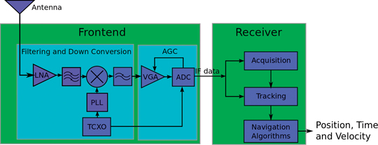
GPS receivers consist of an analog portion and a digital portion: the analog signal, comprised nominally of GNSS signals and white Gaussian thermal noise, is received, amplified, down-converted, and filtered, then converted to a digital signal for processing within receiver acquisition and tracking loops. During signal sampling and quantization by the Analog to Digital Converter (ADC), some quantization losses will occur. These losses depend on the ratio between the ADC’s maximum quantization threshold, L, the number of bits utilized, and the incoming signal standard deviation, σ.
This is where the AGC comes in. In a typical GPS receiver, it sits between the analog portion of the front end and the ADC, as shown in Figure 1. The AGC acts as a variable gain amplifier, adjusting the power of the incoming signal to optimize the L/σ ratio, minimizing quantization losses. This assumes the receiver is a multibit design which is the norm for GPS receivers today.
FIGURE 1. Typical GPS receiver architecture.
When the GPS band is interference free, which should be the norm due to restrictions on emissions in and near the band, the AGC gain depends almost exclusively on thermal noise, since the received GPS signal power level is below that of the thermal noise floor. Since this thermal noise is a physical constant with minimal fluctuation resulting from the span of temperature variations on earth, the primary role of the AGC is to adjust to different active antenna gain values. However, in the unlikely presence of interference the AGC gain drops in response to increased power in the GPS band. Thus, AGC levels may be used to indicate potential interference. Moreover, AGC levels are expected to respond to the interference before receiver performance is compromised, so useful flags may be established, which could provide a warning before a problem exists.
Baseline AGC Data Gathering
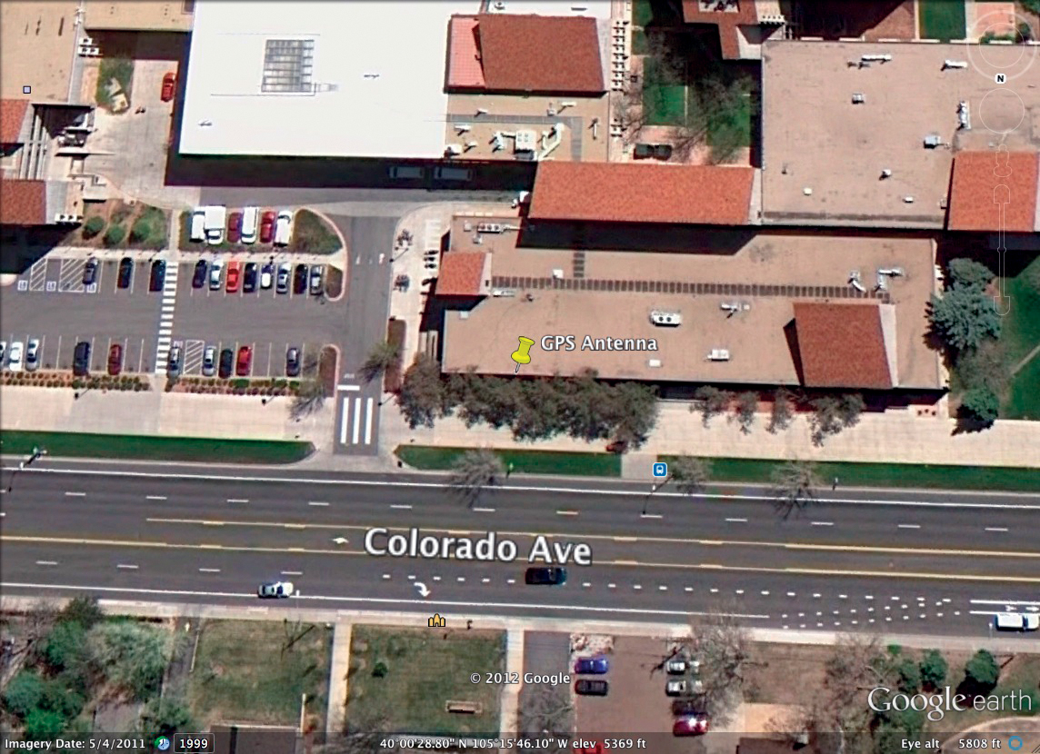
Prior to the spoofer experiment, baseline AGC data were collected for 72 hours using both a survey grade and a mass market receiver. The GPS antenna was located on the roof of the Engineering Center at Colorado University (CU) in Boulder (Figure 2).
FIGURE 2. Antenna location for baseline AGC data collection.
Currently there is no standardization among GPS receivers for AGC reporting units or the measurement itself. Most receivers offer such a metric but it is likely that each needs to be interpreted individually. However, in general this metric provides an indication of the relative gain of the amplifier within the receiver. Should the active antenna be disconnected (loss of gain), the AGC metric will increase showing the increase in internal gain needed to compensate for the loss of the active antenna amplification of the thermal noise floor. Should additional energy be detected in band, the internal gain will decrease accordingly.
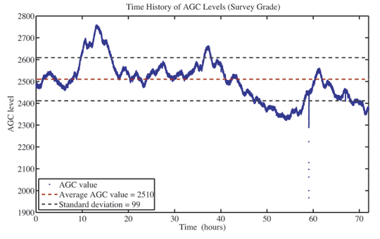
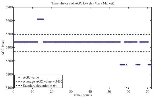
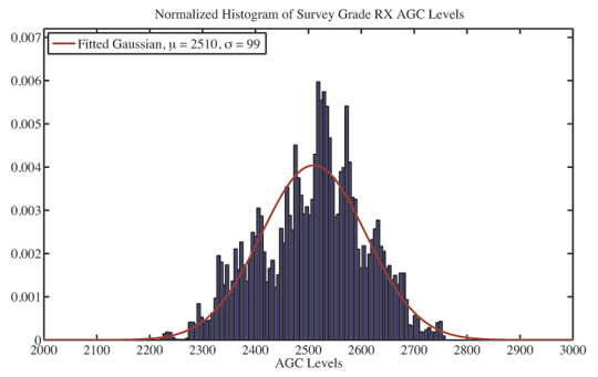
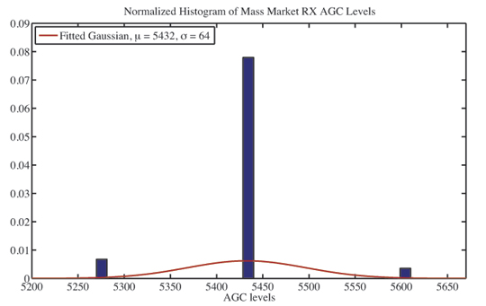
Baseline AGC levels from the survey grade and mass market receiver are shown in Figures 3a and 3b, respectively. The survey grade receiver AGC measurement was more sensitive to changes in the nominal environment; these results will be discussed later in more detail. The mass market receiver provided a much more consistent measure for the entire test period. Interestingly, there was one brief yet noticeable drop in AGC metric from the survey grade and mass market receivers at approximately hour 59 into the collection. Its magnitude was not overly significant, as it did not have an impact on the availability or accuracy of the position solution measurements from either receiver. It is assumed that this is a brief RFI event that occurred during the collection, perhaps from an illegal personal privacy device (PPD) in a vehicle on the nearby road.
FIGURE 3A. Nominal AGC values for survey-grade receiverFIGURE 3B. Nominal AGC values for mass-market receiver.
This RFI event outlier was excluded from the computed mean and standard deviation from the receivers’ AGC data. As shown in Figure 4a, the mean reported AGC gain was approximately 2510, and its standard deviation was approximately 99. For the mass market receiver, the data shows clear evidence of quantiztion in Figure 4b. Here the mean AGC level in this test was approximately 5432, standard deviation was approximately 64. Again, the absolute measures mean little and cannot be compared from various vendors of receivers. It is, of course, possible to calibrate individual receivers and obtain an absolute measure should this be required for a specific application. During the baseline data collection receiver reported position solutions were nominal, with deviations on the order of 2-3 meters in east and north directions, and 5-6 meters in the vertical direction for both receivers. A Gaussian curve was fit to the AGC data and although the data may not be well modeled by a Gaussian, a 2x standard deviation will be used to establish a quick initial flag to indicate potential spoofing/interference.
FIGURE 4A. Histogram of survey-grade AGC data.FIGURE 4B. Histogram of mass-market AGC data.
AGC Reactions to Live Spoofing
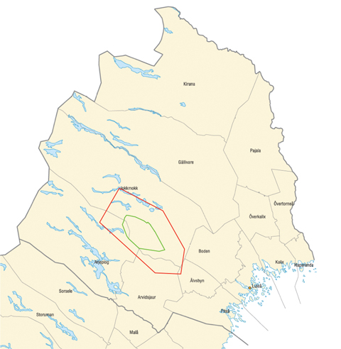
Live RFI or spoofing experiments are quite difficult to conduct due to the global and national legislation protecting the GPS frequency band. Any such experiments tend to be conducted with significant advanced planning and in locations where the testing will have no impact on any system or application which uses GPS outside the test range. Thus, we are grateful to have been able to test the AGC detection of live transmissions in the GPS band. This was done at the Robotförsökplats Norrland test range in Northern Sweden (Figures 5A, 5B, 5C) with the support of the Swedish Defense Research Agency.
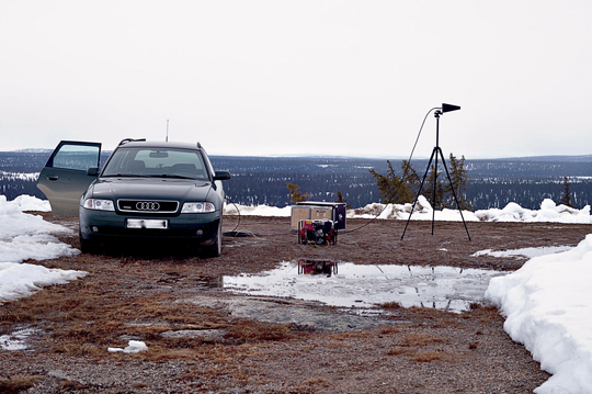
FIGURE 5A Robotförsökplats Norrland test range in Northern Sweden (green outline is the test range and red outline is the flight restriction area, approximate 130 x 70 kilometers).FIGURE 5B Repeater spoofer transmission antenna.FIGURE 5C. Test vehicle
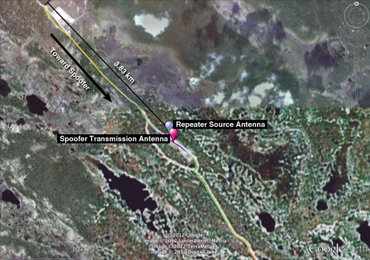
Dynamic GPS receiver measurements (position and AGC) from both the survey grade and mass market receivers were logged in the presence of repeater spoofing. Tests performed involved installing GPS antennas on the rooftop of a vehicle and driving along a 4km stretch of road toward (and away) from a hill top repeater spoofer transmission antenna while logging AGC levels and receiver positions from various GPS receivers. The data from both the survey grade and mass market receivers, used in the baseline collections, will be used here. The repeater spoofer source and transmissions antennas and the road (color shaded by elevation) used to go to/from the spoofer transmission antenna are shown in Figure 6.
FIGURE 6. Google Earth view of testing environment.
The baseline receiver data was used to establish the change in AGC levels necessary to flag potential jamming, spoofing, or unintentional RFI. In order to implement the AGC flag proposed in this paper, a known fixed RF chain (antenna, cable, and front end) would be calibrated in a known non RFI environment and the mean AGC would be established. Given the baseline data collection, a mean value has been established and a 2σ threshold is set as the RFI/Spoofing flag for each receiver. When the AGC drops below this flag, the resulting position/time solution should not be trusted.
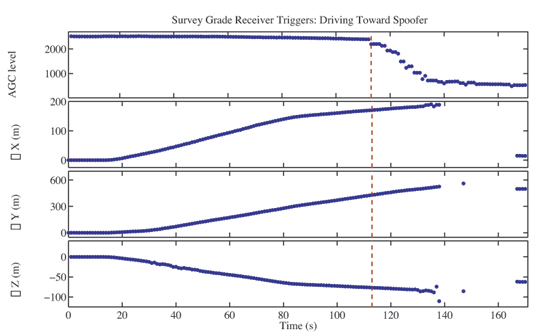
In Figure 7 the measurements (AGC metric and survey receiver reported position) are shown as a function of time as the receiver is driven toward the spoofer transmission antenna. Under nominal conditions (no RFI or spoofing) one would expect a constant “safe” AGC value as well as a smooth gradual change in the reported XYZ coordinates (as the drive maintained a constant speed on the road for the duration of the test). However, as expected, due to the additional power in the GPS band, the AGC gain drops as the receiver gets closer to the repeater spoofer. At approximately 138 seconds the receiver fails to report a position and this continues for the next 30 seconds as the vehicle progresses toward the spoofer transmission antenna. At approximately 168 seconds, the survey receiver is captured and reports the fixed position of the spoofer source antenna despite continually moving toward the transmission source. Although the loss of lock and position jump could be utilized as a flag for spoofer detection, the AGC metric here clearly shows the additional power in the band prior to any corruption of the reported GPS receiver position. If the previously computed threshold is used here, the 2σ trigger occurs as the AGC level begins to drop, significantly before any loss of lock or any change in the position solution resulting from the repeater spoofer.
FIGURE 7. Survey-grade RX AGC/position during drive toward spoofer.
Figure 8 shows this same data for the mass market receiver with similar observations. First, and most importantly, the AGC metric can be used here as a flag well before any corruption of the resulting position solution. The resulting position solution as the receiver becomes “captured” by the spoofer is odd, not going directly to the repeater source antenna location but also not maintaining the true position either. Likely a result of the navigation filtering coupled with individual range measurements transitioning from the true satellite measurements to that from the repeater spoofer. Nevertheless, it is clear from the AGC metric that the receiver output should not be trusted , well before any misleading information is provided.
FIGURE 8. Mass-market RX AGC/position during drive to spoofer.
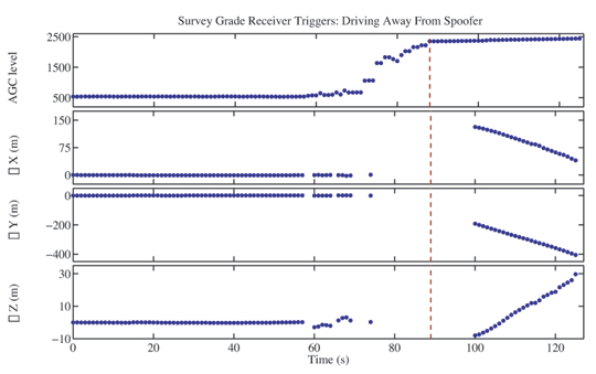
Figure 9 shows AGC levels and reported positions for the survey grade receiver as it is driven away from the repeater spoofer. At the beginning, the receiver is already captured by the spoofer and reports a false fixed position solution even while the vehicle is moving. While in close proximity to the spoofer, the AGC levels are low, attempting to compensate for the additional power in the GPS band. This would be an obvious flag that the resulting position cannot be trusted (all measurements to the left of the threshold are considered untrustworthy). As the receiver is driven away and exits the spoofer’s region of influence, power levels in the GPS band return to normal, the AGC reacts accordingly by increasing its gain, and the receiver begins to report accurate position solutions.
FIGURE 9. Survey-grade RX AGC/position during drive from spoofer.
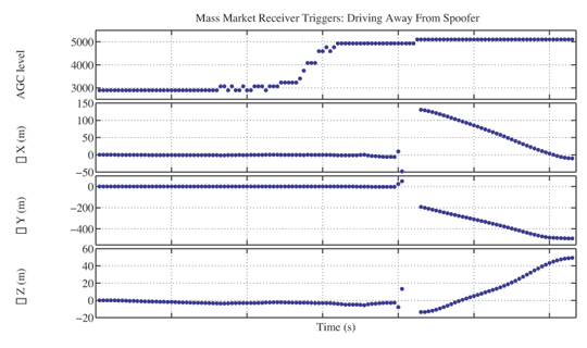
Figure 10 shows this same data for the mass market receiver with similar observations. The AGC metric can be used as a flag indicating the position solution cannot be trusted until the receiver is well outside the range of the repeater spoofer. In this test, the AGC level does not return to a level within the established threshold, indicating that GPS solutions should not yet be trusted. This is likely a result of an overly conservative threshold (perhaps from the poor fit of data which is not well represented by a Gaussian) or perhaps hysteresis or smoothing in the AGC metric for this receiver.
FIGURE 10. Mass-market RX AGC/position during drive from spoofer.
These cases are representative of similar repeater spoofing tests we performed: in all cases this trigger identified potential interference well before the receiver reported false positions with the simple triggers established.
Improvements and Optimizations
These results do demonstrate the power of AGC to detect deception in GPS transmission, rendering these spoofers no more of a threat than the much less sophisticated jammers. However, the spoofer used in this testing was of a simple nature — a repeater spoofer.
The challenge would be to utilize such an approach to detect the most sophisticated spoofing attacks. This should be possible as the underlying thermal noise floor is a physical constant and in order for a receiver to be spoofed additional energy must enter the RF chain which, again, should be detectable. The optimization will come in via establishing thresholds – similar to GPS signal acquisition/detection. One will not want to set such a loose threshold such that frequent false alarms provide little confidence in the resulting position/time solution. Likewise one would not want to establish threshold so loose that the more sophisticated spoofing attacks would be successful. The key is the calibration and assessment of the underlying AGC measurement.
Recall the variation observed in the survey grade receiver data. Was this truly random noise that one must overbound as was done to establish the threshold for the experiments in this paper? And why were the noise levels so different for the baseline AGC collections in the survey grade and mass market receiver? We try to address both of these questions to provide a bit of insight into the advantages and shortcomings of the AGC metric.
First, the AGC measurement across receivers is not equal. In comparing these two receivers, the survey grade receiver has a much higher resolution measurement than that of the mass market receiver. This is obvious from the baseline data which showed little deviation from specific quantized levels in the mass market AGC metric. So although the great majority of GPS receiver already have/report their AGC measurement it may not be of sufficient fidelity for the most sophisticated spoofer detection.
Second, high resolution provides little benefit in a noisy measurement. So there is a pending question if there is a source for the variation in the AGC measurement for the survey grade receiver during the 72 hour baseline data collection – or was it simply a noisy measurement. Past work in this area led to the association of ambient temperature and the AGC measure, but perhaps not in the way one would initially think. Yes, the thermal noise level is dependent on temperature (from kTB), as well as bandwidth and Boltzmann’s constant, but this is really antenna temperature and in this case the correlation is with ambient temperature.
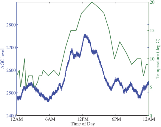
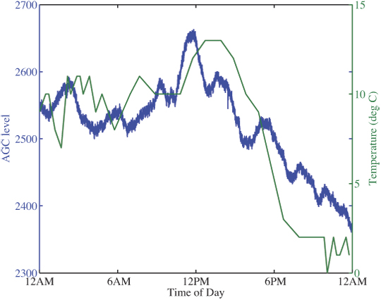
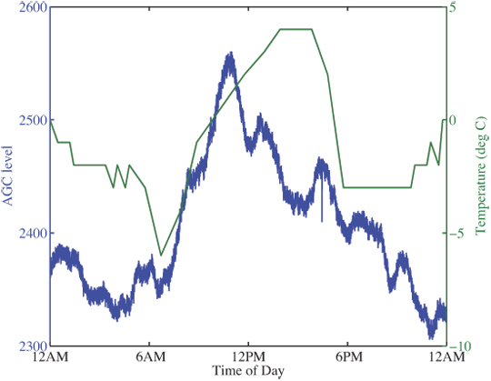
The baseline AGC levels were compared to changes in ambient temperatures in Boulder during testing to determine if observed fluctuations were related to temperature. The weather data were gathered in Broomfield, approximately 10 miles from CU; thus plotted temperatures do not exactly reflect the air temperature at the antenna. However, the data do reflect a correlation between approximate ambient temperature and AGC gain, shown in Figure 11a, b, and c.
FIGURE 11A. AGC measure (survey-grade RX) and ambient temperature, Day 1.FIGURE 11B. AGC measure (survey-grade RX) and ambient temperature, Day 2.FIGURE 11C. AGC measure (survey-grade RX) and ambient temperature, Day 3.
Why does this correlation exist? Why, when the temperature increases, must the gain of the receiver also increase? That may initially appear to be counter intuitive in that one may think higher temperature would result in higher thermal noise. Again, it is important not to confuse antenna temperature and ambient temperature which is the basis for the thermal noise floor. Why then must the receiver provide more gain with higher ambient temperatures? The validated hypothesis is that the antenna is an active design with an internal low noise amplifier. The gain, or really efficiency, of this amplifier is dependent on its temperature (and it is quite small, on the order of a dB). So as the ambient temperature increases the efficiency of the amplifier in the antenna decrease so the receiver is required to put more gain into the RF chain to accommodate.
This temperature correlation is an attempt to illustrate the power of the AGC metric and its potential sensitivity for detection. Other triggering methods, such as comparing current AGC levels with a moving average of previous values, could be implemented depending on desired performance. If such changes can be incorporated and/or calibrated out, we expect the most sophisticated spoofers could be detected coupled with a low false alarm rate.
Conclusion
A trigger based on the AGC, a measure available in a majority of GPS receivers, has been proposed that indicates the presence of potential signal spoofing prior to a compromise in receiver positioning. This proposed trigger is an effective tool for current GPS receivers to establish a low computational complexity measure of confidence of the reported position solution, and may complement other spoofing detection methods. The triggering mechanism may be adapted according to desired sensitivity in AGC changes, thereby either reducing the false alarm rate, or providing a conservative flag of potential RFI. Upon receiving such a flag, other navigation sources may be consulted to determine position, or the trust in the GPS solution may simply be lowered. Thus spoofing would be no more of a threat to satellite navigation/timing receivers than the much less sophisticated jamming.
Acknowledgments
Our thanks to the Robotförsökplats Norrland test range in Northern Sweden and the Swedish Defense Research Agency, particularly Peter Johanson and Mickael Alexandersson (who provided many of the photographs) for supporting the experiment.
Holly Borowski is a Ph.D. student working in the Research and Engineering Center for Unmanned Vehicles at the University of Colorado-Boulder. Her research involves unmanned vehicle path planning for information gathering in uncertain environments.
Oscar Isoz is a Ph.D. student at Luleå University of Technology. He has studied GPS interference detection and localization and is now focusing on radio occultation.
Fredrik Marsten Eklöf is the project manager for NAVWAR research at the Swedish Defense Research Agency.
Sherman Lo is a senior research engineer at the Stanford GPS Laboratory. He is the associate investigator for the Stanford University efforts on the FAA evaluation of alternative position navigation and timing (APNT) systems for aviation.
Dennis Akos is an associate professor with the Aerospace Engineering Sciences Department at the University of Colorado as well as a consulting associate professor with Stanford University and a visiting professor with Luleå University of Technology.
By Nicolas Couronneau, Peter J. Duffett-Smith, and Alexander Mitelman
Cell-phone users are often more concerned about the speed of positioning than the accuracy, making time-to-first-fix the most important factor in a GNSS mass-market receiver’s perceived performance. However, TTFF is generally difficult to characterize and optimize because of the need to encompass a wide range of environments, including indoors.
One method of characterizing the time-to-first-fix (TTFF) is to measure it directly, using a signal generator and a real receiver. This method avoids the approximations of analytical solutions, but it is usually time consuming and it does not provide much insight into the factors affecting the TTFF since it is gen erally not possible to change the receiver’s architecture. Another approach is to use Monte Carlo simulations and a model of the acquisition process. This approach is more flexible than direct measurement, but again it can take a long time to simulate weak-signal environments.
We have developed a third approach based on analytical methods but regulated by measurements of the signal-to-noise ratio in target environments. Using this approach, one can quickly calculate the probability distribution of the TTFF for different signal strengths and acquisition parameters.
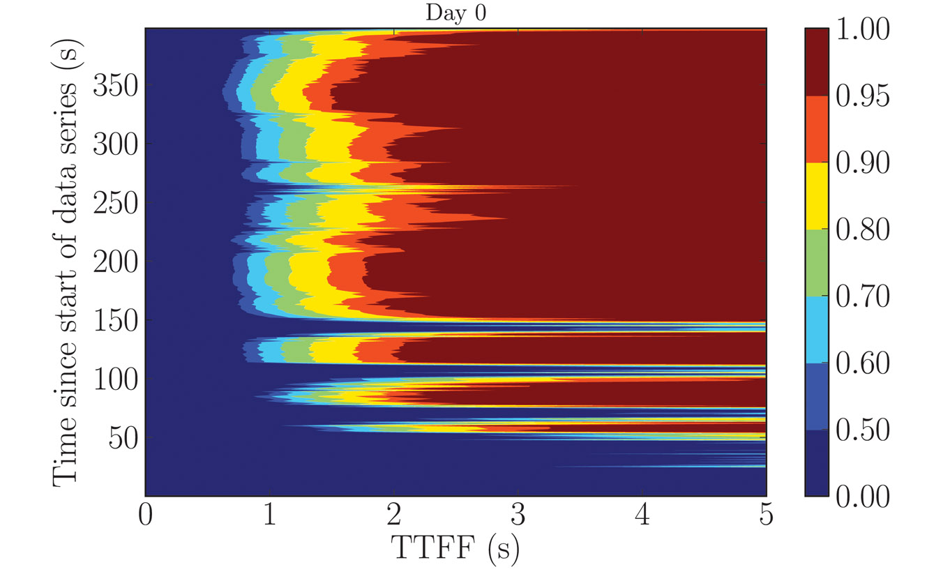
To illustrate this method, we consider a model of an assisted-GPS receiver combined with experimental measurements of the GPS L1 C/A signal taken indoors. The results are presented in Figure 1, where the probability of the TTFF (horizontal axis) is plotted as a function of the time after the beginning of the data series at which the acquisition process started (vertical axis), calculated using a 400-second GPS data series measured indoors. The strength of our approach is that we can quickly calculate the TTFF probability for any given confidence level and it is quite general so that it can be extended to other types of receivers.
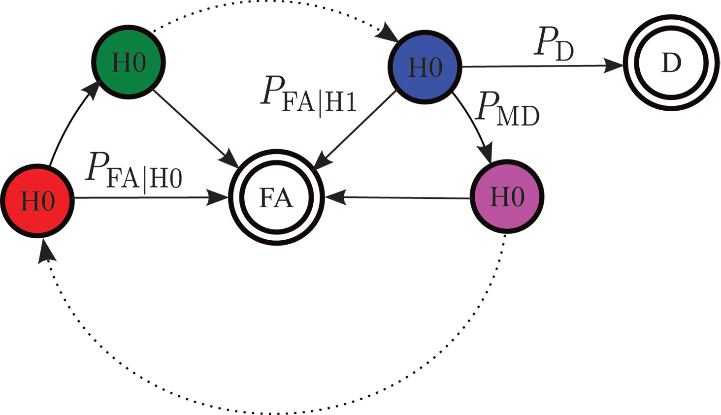
Flow-graph representation of the acquisition process for one channel. FA is the false-alarm state and D the correct detection of the signal from this satellite. H1 and H0 represent respectively states in which the signal is and is not present. PFA|H1 is the probability of false alarm in a window where the signal is present and PFA|H0 the probability of false alarm in a window where the signal is not present. P D is the probability of detection, and PMD the probability of missed detection.Figure 1. The probability of the TTFF (horizontal axis) as a function of the time after the beginning of the data series at which the acquisition process started (vertical axis), calculated using a 400-second GPS data series measured indoors. Note that the colored scale is not linear.
Modeling the Acquisition Process
A GPS receiver must first acquire signals from a sufficient number of satellites before it is able to calculate a position. This search is often the major contributor to the TTFF.
GPS Acquisition Architecture. The acquisition can be represented as the search for a specific, yet unknown, combination of three parameters in a larger search space. These are:
the Gold-code number used to generate the pseudo-random noise (PRN) sequence,
the code phase, and
the carrier frequency offset.
The last of these has contributions from the frequency offset caused by the relative motion of the satellite and receiver (the Doppler effect) and the frequency bias of the receiver’s local oscillator.
In general, signal detection is performed by correlating incoming signals with a local satellite signal replica for every combination of parameters in the search space. The correlated signal is then integrated and a “hit” is declared if the integrated value crosses a predetermined threshold. The time required to test for the presence of a satellite signal for each combination of parameters is called the dwell time. We suppose here that this is approximately equal to the integration time.
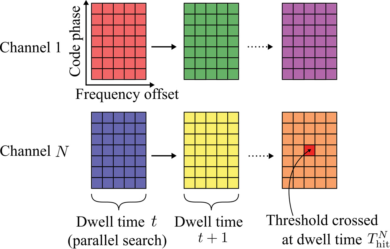
GPS receivers usually include some degree of parallelism. We consider a receiver having N channels, each channel dedicated to searching for signals with a different PRN sequence. Within a channel, the frequency and code-phase search spaces are further divided into several windows. We assume that all the parameter combinations within a window are searched in parallel, that is, within a single dwell time. This model of the acquisition process is outlined graphically in Figure 2.
Figure 2. An illustration of the acquisition process. The large colored rectangles represent the search windows and the inner smaller rectangles represent the different combinations of search parameters.
Parallelism can be implemented in hardware using massively parallel correlators or in software using fast Fourier transform-based techniques. The details of any particular implementation are not relevant here; only the number of channels, the number of windows, and the sizes of the global search spaces are needed.
Acquisition Time Probability Distribution. The flow-graph method provides a graphical representation of the acquisition process. An example is shown in the Opening Figure. Each node represents a state of the acquisition process at the end of a dwell time. The lines joining the nodes represent the transitions of one state to another with the given probabilities. Typical states during acquisition are false alarm, missed detection, correct detection, and correct non-detection.
The flow-graph method has already been applied to the GNSS acquisition problem, in particular for calculating the mean acquisition time of a signal in a GNSS receiver. Here we extend that work by considering the acquisition of all the satellites required for a position fix and, by deriving full probability distributions, we establish a model of an assisted-GNSS receiver.
The opening figure shows the various probabilities of transition that can be calculated from detector statistics.
Flow-graphs rely on the properties of the probability generating function (PGF) of a random variable. A PGF makes it straightforward to calculate the probability distribution of the total duration of a sequence of events of random durations since the PGF of the sum of random variables is simply the product of their PGFs. It is also straightforward to calculate the mean and standard deviation of a random variable directly from its probability-generating function.
Aside from these properties, PGFs are less convenient and less intuitive than probability distribution functions. A generating function does not provide a direct calculation of the probability of an event, unlike a distribution function. For instance, calculating the acquisition time at an arbitrary confidence level (for example, 90 percentile) requires a contour integral over the PGF. Furthermore, some operations are easier to perform on density functions, for example, calculating the probability of simultaneous events.
It can be shown that the probability mass function of a discrete random variable can be approximated from its generating function using a discrete Fourier transform. This property forms the basis of our method: using the fast Fourier transform (FFT), we can quickly calculate the entire acquisition probability distribution associated with the generating function of a flow-graph.
Assisted-GPS Model
We now focus on the specific architecture of an assisted-GPS receiver, such as is commonly found in cellular phones. In this type of receiver, the TTFF can be shortened by performing the acquisition in two steps.
The acquisition starts by searching for any satellite signal in a full search space in which every parameter takes its full range of values. The Doppler frequency of the first satellite acquired can be calculated using assistance data and then removed from the observed frequency offset to give the contribution to the frequency offset caused by the receiver’s clock frequency offset. This is common to all search channels and can be removed from the remaining search spaces.
The second stage of the acquisition is thus performed for the remaining satellites over a reduced search space.
Stage 1 Full Search Space. The first threshold crossing for a single satellite is characterized by the time-to-first-hit (TTFH). Using an FFT, we can calculate the distribution function P(Thitfull ⩽ t) of the time-to-first-hit Thit(k) of the kth channel.
Mathematically, the time to first hit across all N channels, Thitfull, is the minimum of {Thit(k)}, whose distribution function is calculated by:
We assume that we have no means of detecting a false alarm at this stage and so the frequency parameter of the first threshold crossing is used to calculate the receiver’s clock frequency offset. This crossing may, of course, be a false alarm, and we take this into account later.
Stage 2 Reduced Search Space. At the reduced-space stage, the goal is to calculate the probability of having acquired M satellites out of N channels. The value of M depends on the number of pseudorange observables needed to solve the position equation. High-sensitivity assisted receivers that do not have signal tracking loops can only measure fractional pseudoranges together with an uncertain number of integer code periods. Using a coarse position estimate of the receiver, this uncertainty can be resolved, and a 3D position fix obtained, by using M = 5 satellites.
Calculating the detection probabilities at this stage involves some combinatorial arguments. In the following, (Ωm) represents the set of all combinations of m elements from the set Ω. For example, if Ω = {a, b, c}, then (Ω2 ) = {{a,b}, {b,c}, {a,c}}.
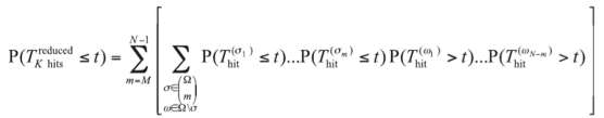
The probability of having “hit” at least M signals out of N channels at time t is given by
In this equation, Ω = {1, …, N} represents the set of the receiver’s channels and Thit(k) is the time to first hit of satellite k. Because each satellite is received with a different signal strength, these random variables have different distributions for every satellite.
The probability of having correctly detected at least M satellites before time t, P(TDreduced ⩽ t), is calculated by enumerating all the possible combinations of hit and detection events. The probability of having at least one false alarm before a given time t, P(TFAreduced⩽ t), is simply calculated by taking the difference between the probability of a hit and the probability of detection.
The number of possible combinations grows quickly with the number of channels. For an 8-channel receiver, there are 35 combinations, and for a 24-channel receiver there are 8,855 combinations. If the number of summations is becoming too computationally demanding, one solution is to form sets of signals with similar strength, and perform the combinations over these smaller sets with an appropriate weighting. Within a smaller set, all the signals have the same signal strength and acquisition times have the same probability distributions — a situation that is similar to calculating the order statistics of a random variable, which is not problematic in the case of identical distributions.
TTFF Probability Distribution
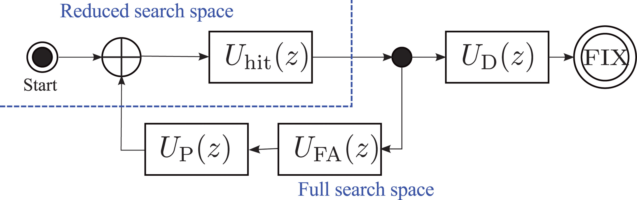
The last step before obtaining an expression for the TTFF distribution is to combine the two stages of the assisted acquisition. The total acquisition time is the sum of the time to first hit in the full-space stage and the time to the correct detection of M satellites in the reduced-space stage. This sum is easily calculated using generating functions, with the corresponding flow-graph represented in Figure 3.
Figure 3. Overall flow-graph of an assisted receiver. Uhit(z), UD(z), UFA(z), and UP(z) are the generating functions of the time to first hit in the full-space stage, the time to detections in the reduced-space stage, the time to a false alarm in the reduced-space stage, and the penalty time to recover from a false alarm, respectively.
Using the inverse of the FFT method presented above, we calculate the generating functions of the time to first hit in the full-space stage, Uhit(z); the time to M detections in the reduced-space stage, UD(z); the time to a false alarm in the reduced-space stage,UFA(z), and the deterministic time penalty to recover from a false alarm,UP(z).
Modeling false-alarms demands special attention. There is little information in the literature about the detection of false alarms in assisted-GPS receivers. One solution could be to detect a large residual error at the output of the positioning algorithm. Here, we take an easy path and simply introduce a penalty time, TPenalty, to represent the (deterministic) time needed to recover from a false alarm. The penalty time should be chosen to represent the behavior of a specific receiver.
For GNSS receivers capable of tracking the signals, the full pseudorange can be recovered after detection of a synchronization word in the navigation message. The duration of the tracking stage is a random variable, since the tracking can start at any position in the navigation message. Although we have not investigated this situation in more detail, we suspect that the tracking stage can be simply modeled by a uniform probability distribution. The length of this distribution depends on the navigation message structure and the amount of navigation data needed by the receiver to obtain a full set of decoded data. A new block can be added to the flow-graph in Figure 3 using the generating function of the uniform distribution, and the TTFF for a standard GNSS receiver can then be calculated.
Experimental Results
We analyzed the TTFF with the signal strengths measured in an office environment.
A picture of the office is shown in Figure 4. One side of this office has a window, but the sky view is obstructed by a large building a few tens of meters away. There is no direct line of sight to a satellite, although the window may allow some strong reflected signals to get in to the office.
Measurement of Weak Signals. Direct measurement of the strengths of indoor signals can be challenging since the signals are often too weak to be tracked reliably. We used a Nordnav R30 dual-input receiver with one input connected to an outdoor antenna mounted on the roof of the building and having an unobstructed view of the sky. The other input was connected to an antenna in the office. We used the tracking information from the stronger outside signal to track the indoor signal.
The signal carrier-to-noise density ratio (C/N0) was recorded for 400 seconds, starting every day at the same sidereal time, for six consecutive days.
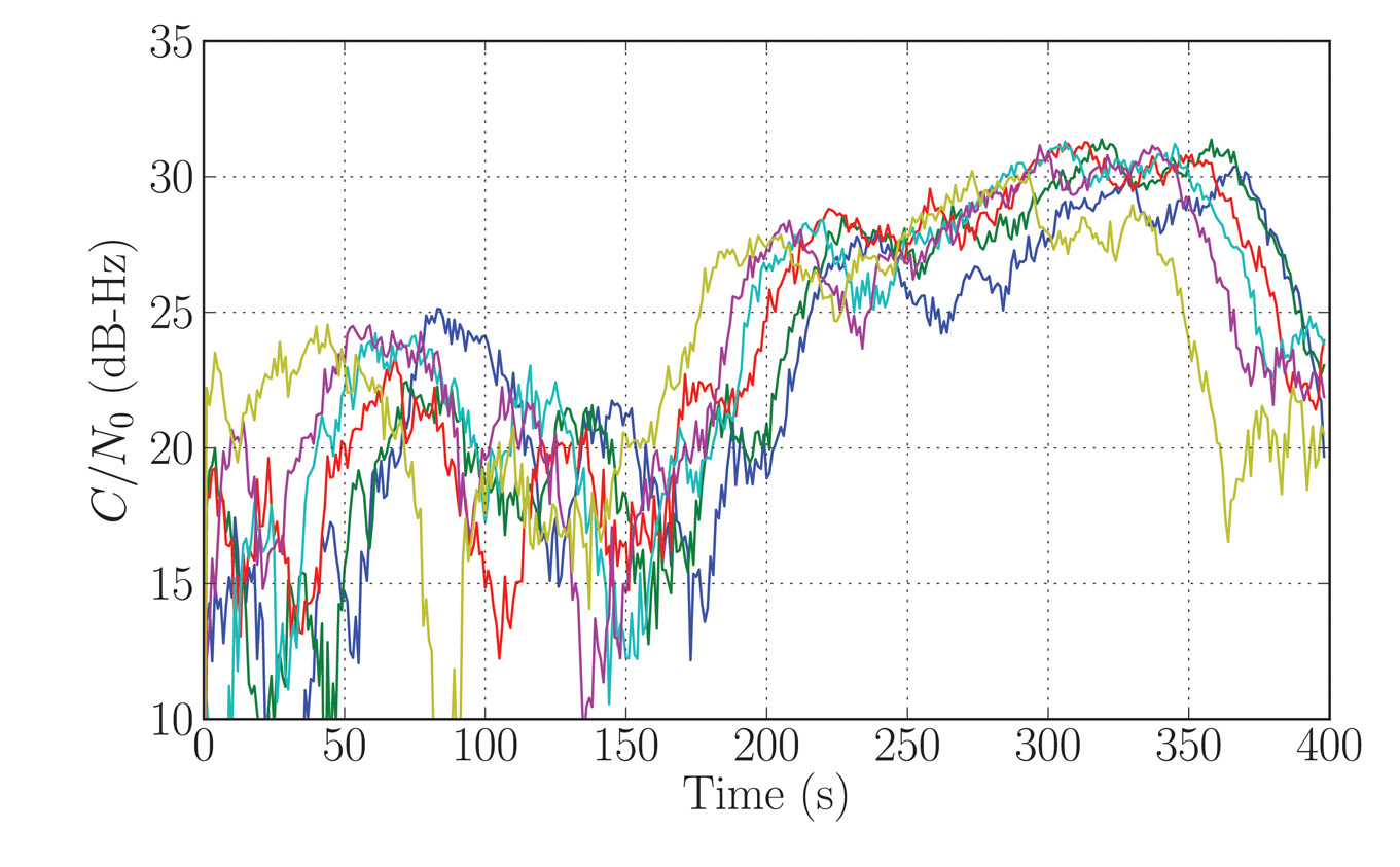
Figure 5 shows the signal strength for one particular satellite (GPS PRN9). We see that the signal strength follows a similar pattern every day. This is representative of a multipath fading environment: the signal coming from the satellite is scattered in the office, and the resulting signals interfere constructively or destructively, depending on the phase difference between the different paths. The overall signal strength is therefore related to the relative position of the satellite which, for GPS, is about the same every day at a given sidereal time.
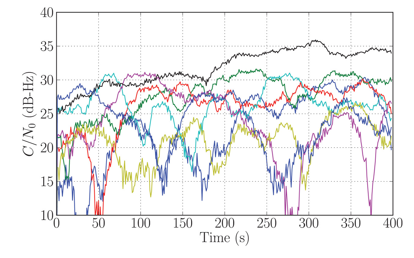
The variations of the signal strengths of all the observable satellites show fading patterns which are uncorrelated, as we expect the satellites to be spread across the sky (see Figure 6). It is difficult, if not impossible, to predict the distribution of signal strengths at any specific instant, and so the TTFF varies depending on the instant at which the acquisition process begins.
Figure 5. Indoors signal strength (C/N0) for satellite PRN09. Each colored curve represents the signal strength measured on a different day, starting at the same orbital time.Figure 6. Measured C/N0 for all observed satellites during the first day of recording.
TTFF Indoors. We now apply the signal strength measurements (Figures 5 and 6) to the TTFF calculation method presented above. This allows us to determine the probability of the TTFF as a function of the starting time of the acquisition since the beginning of the data recording.
We chose the detection parameters as follows: the coherent integration time was 1 millisecond, the non-coherent integration time was 300 milliseconds, the threshold was set for a probability of false alarm of 10–6, the time offset of a code phase was between 0 and 1 milliseconds, the penalty time for a false alarm was set to 600 milliseconds, and five satellites were required to solve the position equation. The ephemeris, a coarse position within 150 kilometers of the true position, and a coarse time within 30 seconds of the GPS system time were provided by the assistance data.
The results (see Figure 1) provide some insight into the acquisition process.
We can discern two patterns in the TTFF distribution. During the first 150 seconds of the analysis, that is, if a real receiver had started acquisition during that time, the TTFF showed large variations. This was caused by the multipath. The fading of the signals from the various satellites, although uncorrelated, led to severe degradation of the TTFF when the acquisition was started during a combination of strong fades. In our analysis, we have made the simplifying assumption that the strength of any particular satellite signal remains constant over the acquisition period.
After the first 150 seconds, the TTFF became more nearly constant. On examining the C/N0 time series, it was clear that the reason was the appearance of a signal from the satellite with PRN 27 (black curve in Figure 6) which was consistently stronger than the remaining signals after 120 seconds. This satellite had the highest elevation (more than 60 degrees) and the reception was probably by transmission through the ceiling of the office. In this situation, the phase difference between the reception paths was small, hence there was little fading. This single satellite significantly improved the TTFF, in particular by shortening the time of the first stage of the assisted-acquisition process.
It can be shown that the distribution of the acquisition time of a satellite, at a given starting time, can be approximated by an exponential distribution. This distribution explains the non-linearity of the relationship between the TTFF and the probability of fix, as observed in Figure 1. The non-linear effect becomes important when calculating the TTFF at a given performance level. In our example, the 50-percent probability of fix was about 1.2 seconds. Moving the requirement to 90 percent made it about 2 seconds, and 95 pecent about 2.5 seconds.
Conclusions
In presenting a method of calculating the distribution of the TTFF representative of a mass-market receiver indoors, we have seen how existing techniques can be extended and combined to provide an analytical model for assisted receivers. Power measurements of real signal show how the TTFF can vary depending on the combination of signal strength at the time the acquisition process is started. This suggests that an improved strategy for acquisition in large search spaces might be to start two or more independent acquisition processes, separated by, say, 1 second, in order to benefit from the advantage of one of the signals appearing strongly after a fade.
The lead author gratefully acknowledges support for this research from Cambridge Silicon Radio, CSR plc.
Nicolas Couronneau is a Ph.D. student at the Cavendish Laboratory, University of Cambridge, UK. He graduated as an electrical engineer from Supélec, France. His research interests are in the area of probabilistic methods applied to the acquisition of GNSS signals.
Peter J. DufFett-Smith is reader in experimental radio physics at the Cavendish Laboratory. His Ph.D. was in radio astronomy. He is the founder of Cambridge Positioning Systems Ltd. and, with others, invented the Matrix positioning method and Enhanced-GPS technologies. He holds more than 20 patents, and is a consultant to the GPS Group at Cambridge Silicon Radio.
Alexander Mitelman received his Ph.D. degree from Stanford University in electrical engineering. His research interests include signal-quality monitoring, algorithm and system design, and the development of testing methodologies for GNSS and hybrid systems.
For the past several months, controversy has raged over the revelation that Apple and Google tracked mobile subscriber location movements and stored that information in an unencrypted file on the handset, where it was potentially vulnerable to hacking and other inappropriate usage. The resulting Location-gate scandal highlights the sometimes tenuous control of mobile subscriber information versus the business objectives of dominant platform and applications providers. These business objectives may include immediate revenue opportunities from the subscriber being tracked or broader self-interest initiatives, such as collecting marketing data that may be valuable to third parties like advertisers, or building subscriber-reported Wi-Fi access point databases.
Furthermore, while much has been written about the privacy impacts of the collection and use of consumer location information, few articles have clearly outlined the technologies behind Apple and Google’s tracking activities. It is important to fully explore and understand these technology methods, and how they differ from other location technologies in use, in order to properly evaluate the threat posed by Location-gate and to develop responses that maintain privacy while enabling the benefits of location-based services.
Location, Tracking, and Storage
iPhone and iPad subscribers had previously been aware that Apple tracked their location via GPS, because the company notified subscribers when an app required the use of GPS to identify location, and asked them to opt-in. However, soon after Location-gate erupted, Apple’s vice president of software technology, Bud Tribble, testified to Congress in May 2011 that Apple also had been tracking device locations over time using triangulation between nearby Wi-Fi access points and wireless base stations. Triangulation is the moderately accurate method in which the mobile device measures the nearby cell site or access point identifications and possibly signal strengths, typically pinpointing device location to within a few hundred meters.
Following this revelation, Apple’s initial response was that “users are confused” and that it was simply “maintaining a database of Wi-Fi access points and cell towers around your current location…to help your iPhone rapidly and accurately calculate its location when requested.” Soon after Apple location tracking activity was revealed, it became known that Google was doing essentially the same thing, although to a slightly lesser degree (Android phones stored only the 50 most recent coordinate fixes and up to 200 Wi-Fi access-spot locations), and using a similar triangulation method without the subscriber’s explicit knowledge. Google Android devices also have GPS capability.
Why, if both OS providers embedded or leveraged GPS in their phones, would they resort to a less accurate location method, triangulation?
Neither company has provided an answer. We know that the triangulation method uses less battery power than GPS, conserving battery life for other uses while filling in performance holes for GPS in urban and indoor environments. Also, unlike with GPS, mobile subscribers are either not able to disable triangulation or must disable it separately. More relevant is the fact that triangulation allowed the OS providers to identify location automatically and track it over time in the background without the subscriber’s knowledge, for purposes such as building and maintaining a subscriber-reported database of Wi-Fi access points.
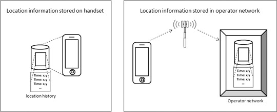
From a privacy perspective, there is a dramatic difference between tracking someone’s location over time (the bread crumb trail that Apple and Google used), versus locating one’s position for a specific purpose and handling the location information only within the confines of a secure wireless network. Useful applications that are universally accepted, such as E911 for safety-of-life situations, employ the latter method.
Other players in the mobile ecosystem, such as wireless network operators, have collected subscriber location information as well, but not by storing it in the device as historical files in the same way that Apple and Google did. Some information exists on the network side in association with billing records for calls (call detail records or CDRs), but this is not bread-crumb tracking of cell-IDs. E911 calls have records stored for use by public safety agencies, but most users never make an E911 call. Other messages containing coarse location may exist on a transitory basis (for example, location area updates), but these are not typically aggregated or stored for later processing.
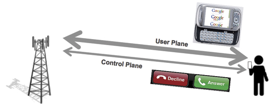
Depictions of location information stored on handset and in operator network.
Alternative Geo-Location Methods
There exist location methods that provide far greater privacy and security than the location tracking and handset storage that Apple and Google have utilized. Standard methods exist for performing location using the wireless service provider’s network elements. These are called control-plane methods, which follow standards developed by 3rd Generation Partnership Project (3GPP) and 3GPP2. Other standard methods exist using IP transport from the client phone to a location server. These are called user-plane methods, such as the Secure User Plane Location (SUPL) standard from the Open Mobile Alliance (OMA). Both control- and user-plane location standards incorporate mechanisms for data security and user privacy. These standard control- and user-plane methods differ from the proprietary methods used by many client applications and OSs, which are inherently user-plane in nature but with non-standard implementations.
Methods using a client application with handset-based location on the mobile device, also called user-plane methods, bypass the carrier’s wireless network elements and instead rely on an IP connection to transmit information from the client application to a server on the Internet. These user-plane location methods, such as client applications for handset-based A-GPS, as discussed, are already widely in use for location-based services. Handset applications are inherently vulnerable to hacking and privacy intrusions, as the recent spate of mobile viruses on Android has highlighted.
A-GPS is highly accurate at identifying location in direct line-of-sight conditions with the satellites (open sky conditions), as found in suburban and rural areas, but performs less well in challenging dense urban and indoor environments. GPS in the phone can be easily disabled by the end user, and the receiver chip in the handset can cause significant battery consumption when used in demanding applications, such as navigation and monitoring geo-fences. A-GPS, as used by wireless network operators for navigation and other location-based services, does not usually store unencrypted files of historical location information in the handset, as Apple and Google did.
Alternative, network-based, or control-plane, methods make use of the wireless services provider’s network elements to keep location information wholly behind the security of the operator’s firewall, employing highly standard protocols for security and privacy. Control plane location methods are used for today’s safety-of-life applications, like E911, where security and privacy are prime considerations.
One example of a network-based location technology that can work in control-plane is RF pattern-matching (RFPM), which is the only high accuracy, software-based, scalable location solution that requires no additional hardware changes/additions to the mobile device or at the base stations. It compares mobile measurements (signal strengths, signal-to-interference ratios, time delays, and so on) against a geo-referenced database of the mobile operator’s radio environment. RFPM boasts a 100 percent security record for subscriber mobile location information it produces, for critical applications such as E911 emergency call and law enforcement location applications.
Location information for growing consumer uses deserves the same privacy and security protections that other standards-compliant control-plane solutions provide for today’s mission-critical and safety-of-life location applications. RFPM works extremely well in non line-of-sight conditions such as dense urban and indoor environments, where GPS-based solutions face challenges. RFPM also offers low battery consumption and geo-fencing capabilities, which makes it ideal for providing location for the growing opportunity in location-based advertising and other location-based services (widely believed to be the true driver behind Apple and Google’s location tracking activities).
As Location-gate clearly illustrates, there is no shortage of methods to identify and track one’s location via mobile device. Now that the issue has been raised, it is imperative that the entire mobile ecosystem — network operators, OS providers, regulators, and subscribers — clearly understand what methods are used, when one’s location is being identified and tracked, and what is being done with that data. Breadcrumb trails are useful if you’re trying to find your way out of the forest, but not if Big Brother is tracking you.
Marty Feuerstein is chief technology officer of Polaris Wireless, where he leads research into new products, algorithms, system performance, and regulatory activities. He has a Ph.D. in electrical engineering from Virginia Tech.
The U.S. Departments of Defense and Transportation declared their strong opposition to the proposal of LightSquared Subsidiary LLC to operate a nationwide broadband service within the spectrum immediately adjacent to GPS signals, in a letter sent on June 14 to the National Telecommunications and Information Administration (NTIA). The agencies acted on behalf of the on behalf of the National Executive Committee for Space-Based Positioning, Navigation, and Timing, which they are responsible for co-chairing.
The Departments asked the NTIA administrator to advise the Federal Communications Commission (FCC) to continue to withhold authorization for LightSquared to commence commercial service per its proposed deployment of a terrestrial service within the 1525-1559 MHz bands. LightSquared’s proposal is to deploy a network of 40,000 base stations along with some satellite coverage over 139 major markets in the United States.
According to their official statement, “The Departments continue to support the National Broadband Plan, but cannot do so at the expense of a global, ubiquitous utility such as the Global Positioning System. The Departments encourage further assessment of any alternative spectrum and/or signal configuration plans.”
The DoD/DoT letter was sent just prior to the original deadline for the final report of the Technical Working Group commissioned by the FCC to research and recommend on this matter. Certainly, the respective signers were cognizant of the contents of that report, at least on the test results regarding interference with GPS. As it turned out, on June 15 LightSquared asked for more time, and was granted a two-week extension. The final report was filed with the FCC on June 30.
The Departments’ position followed an interagency review of the findings of the National Space-Based Positioning, Navigation, and Timing Systems Engineering Forum (NPEF), tasked to assess the GPS impacts of LightSquared’s deployment plan as originally filed. The NPEF determined that, if permitted to operate as originally planned, LightSquared’s signals would significantly interfere with GPS users and, as a result, impact national security, economic security, and public safety nationwide. The NPEF report served as working material for the TWG report.
The NTIA Administrator forwarded the letter and report to the FCC Chairman on July 6. These materials can be found at www.PNT.gov.
Using the Augmentation System with GPS-Equipped Mobile Phones
By François Boullete, Boris Kennes, Michaël Mastier, and Lee Banfield
GPS corrections from the European Geostationary Navigation Overlay Service can improve the positioning accuracy and user experience of GPS-enabled mobile phones, even if EGNOS satellites are not visible and even when the GNSS chipset in the phone does not support satellite-based augmentation systems.
Today, more than 20 percent of mobile phones in use in Europe include a GNSS chipset, and the penetration is expected to exceed 50 percent in the next 5 years. Despite its success in other sectors such as agriculture since the launch of its Open Service in October 2009,
EGNOS has received limited adoption in location-based services (LBS) and consumer applications, due to two main obstacles. First, the signals from the three EGNOS geostationary satellites that are easily received in open-sky environments are difficult to receive in cities, due to masking by buildings. Second, most GNSS chipsets embedded in today’s mobile phones are GPS-only without SBAS support, or use SBAS for ranging only, a function not supported by EGNOS at this stage.
The European GNSS Agency (GSA) and the European Commission (EC) supported the work described here to provide mobile phone operating system and application developers with a library of functions to allow them to benefit from EGNOS in all their applications. It works by receiving correction data via mobile communication networks when EGNOS satellites are not visible to the user device and even when using a standard GPS chipset, overcoming these two main obstacles for adoption.
Targeted mobile operating systems now include Nokia Maemo, Google Android, and Microsoft WinMobile. Further work will extend to this list to other compatible platforms.
This article demonstrates the feasibility and shows the performance of a software-based EGNOS solution and seeks to create awareness among mobile operating system and application developers on EGNOS.
User Benefits and Constraints
Although the sources of GPS positioning errors in urban areas are mainly due to multipath and GPS satellites availability, SBAS corrections on GPS satellites clocks and orbits and ionospheric correction model can still add value in case of moderate multipath environment characteristics. Although GPS stand-alone accuracy is nowadays generally sufficient, it is expected to degrade in the next couple of years as solar activity increases. Availability of free EGNOS corrections delivered via the mobile communication network will help maintain accuracy during these high solar activity periods.
The limited visibility of EGNOS satellites in urban areas requires the use of the mobile communication network to retrieve the EGNOS corrections. This can be perceived at the first sight as a drawback to the proposed solution as it involves communication costs. However, the required bandwidth is negligible compared to today’s mobile applications such as music and video streaming; further, mobile operators increasingly offer smartphones with unlimited data-access packages.
Implementation Overview
Implementation of EGNOS in current-generation mobile phones requires the introduction of a new library of functions at the software level that will allow application developers to get the best possible accuracy in their application regardless of the underlying algorithms used for position calculation. Such a library of functions can eventually be integrated directly in the application programming interface (API) of the phone operation system. At this point, application developers will simply request a position using the API, and the API will return the EGNOS improved position.
The main computations performed by this EGNOS library (see Figure 1) can be summarized as:
Reception: the GPS user position, satellites used, and their elevations and azimuths in NMEA format are requested to the phone’s GPS chipset, and the EGNOS correction message and Klobuchar ionospheric model parameters are received from a distant server (for example, EGNOS Data Access Service EDAS) using the communication link available at the mobile phone;
Preparation: collected input data are decoded and prepared for next step;
Calculation: the new position corrected by EGNOS is calculated by re-creating the line-of-sight or design matrix (using user position and satellite geometry), applying the EGNOS fast, long-term (including clock), and ionospheric corrections (included in the EGNOS message) and subtracting the Klobuchar ionospheric correction that was (assumed to be) applied at chipset level;
Output: the EGNOS corrected position is encoded in NMEA format and returned to the application.
Figure 1. Overview of EGNOS library implementation.
Data Access via the Internet
The EGNOS correction message and Klobuchar ionospheric model parameters are requested by the mobile phone to a distant server. Although the parameters and ephemeris data are stored on the phone’s GPS chipset once it has decoded the messages from GPS satellites, this data is not made available to other phone applications, hence the need to recover it from a remote source. Today, two alternative servers are available: the EGNOS Data Access Server (EDAS) developed by the EC and Signal-in-Space through the Internet (SISNeT) developed by the European Space Agency (ESA).
SISNeT’s advantage is the simplicity of the message (hundreds of bits per second) and the availability of specific functions that allow requesting all the necessary data for our application. However, SISNeT messages are produced from EGNOS signals in space, not from the ground segment: an EGNOS receiver installed at ESA’s ESTEC center receives the signals, demodulates them, extracts the correction message, and re-broadcasts it via the Internet. The reliability and availability of this approach depend upon the good reception of EGNOS signals at this site. Interference or EGNOS broadcast failure could disrupt service.
Unlike SISNeT, EDAS takes the EGNOS correction message directly from the EGNOS system, which guarantees higher service reliability and availability. Nevertheless, the EDAS message is complex and contains much more than the data required for the present application (hundreds of kilobits per second). Therefore a direct connection to EDAS would be inadequate. As a result an EDAS proxy needs to be interfaced between the EDAS server and the mobile platform in order to filter the data flow and extract only the required data. This proxy provides the same kind of messages and functions as SISNeT, whose specifications are ideal for such an application, however it is using data directly from the EGNOS system and not from EGNOS signals in space, improving reliability. In addition, planned EDAS improvements include the provision of such a simplified service directly from the server, removing the need for a proxy.
Independently of the data server used, the mobile platform must retrieve the EGNOS correction messages, and the Klobuchar ionospheric model parameters. The correction message is composed of a number of different message types (MT) as defined in the SBAS standard established by the International Civil Aviation Organization. For our application, the most important messages are:
MT1, the PRN mask that shows to which satellites (PRN) the data contained in the other, subsequent messages are related;
MT2-5, containing data to correct rapid variations in the ephemeris and clock errors of the GPS satellites. The important bits for us in these messages are the fast corrections for each satellite used to calculate the user position;
MT25, with data to correct long-term vari
ations in the ephemeris errors and clock errors of the GPS satellites;
MT18, the ionospheric grid points (IGP) mask that associates ionospheric corrections in MT26 with the IGPs to which they relate;
MT26, providing data to compute the ionospheric corrections for the IGPs present in the IGP mask. In particular it contains the grid ionospheric vertical delay.
The eight Klobuchar ionospheric model parameters must also be obtained from the distant server (using, for example, the GPS_IONO request with SISNeT).
Corrections from GNSS Chipset
The correction algorithm on the phone takes the original position provided by GNSS chipset and identifies the GPS satellite measurements which were used in this computation. It then determines a pseudorange correction for each of the GPS satellites used, and using knowledge of the user-satellite geometry, translates these to a combined position-domain correction.
Most mobile phones’ operating systems allow access to the NMEA sentences from the GNSS chipset using native API functions, for example, onNmeaReceived() with Google’s Android. In order to apply the EGNOS correction algorithms developed in this paper, the minimum required NMEA sentences are GGA, GSA, and GSV.
To construct pseudorange corrections, the Design matrix containing of line-of-sight vectors to the satellites is reconstructed using the elevation and azimuth data. All EGNOS corrections for the satellite orbit and clock errors and the ionospheric delay are applied in this range domain. The algorithm assumes that the Klobuchar model will have been applied to correct for the ionospheric delay in the original GNSS chipset positioning solution. Therefore it provides an adjustment to this original correction to exploit the greater accuracy of the EGNOS ionospheric data. Finally these range corrections are propagated into the position domain using the Design matrix. This provides a 3-dimensional position shift to apply to the original chipset position.
Implementation with Google’s Android
To obtain NMEA strings from an Android phone requires the ‘onNmeaReceived’ function, a function of the LocationManager class. The LocationManager uses the function ‘requestLocationUpdates’ to get a continuous update of the position input, which in this case is GPS. To implement the LocationManager, a LocationListener must be implemented either by the current activity or as a variable. The ‘onNmeaRecieved’ function will be called every second from the instant the Android’s GPS is switched on. The function provides the NMEA strings with a timestamp using the phone internal clock. This timestamp is not derived from GPS and should be used only for logging.
The HTC Legend produces the $GPGSV, $GPGGA and $GPGSA messages that are needed for the application. The Legend also produces $GPRMC and $GPVTG strings. The $GPGSV provides the elevations and azimuths needed for the algorithm, the $GPGGA provides the time, original position and number of satellites in the fix and the $GPGSA provide the PRN numbers of the satellites used in the fix.
For the present testing, necessary data are received via a TCP/IP connection to the SISNeT server (the EDAS proxy server described previously can be used in exactly the same way). For a snapshot solution a continuous connection is not needed and all the information is collected via ‘GETMSG’ and ‘GPS_IONO’ calls. ‘GETMSG’ calls get the last of a specific message type going back up to 30 messages. The types 0,1,2,3,4,5,18,24 and 26 were needed to provide the information for the position domain correction matrices. Only the last message types 0,1,2,3,3,4,5 were needed with type 18 needing 4 and many more of type 24 and 26.
The ‘GPS_IONO’ message gets the current Klobuchar values. By asking for all of the specific message types, almost instantly all the information is gained without having to wait for the 3 minutes Ionospheric grid cycle (message types 18 and 26) and the variable speed, dependant on number of satellites, complete slow correction set. Once the data has been downloaded from the server the connection is closed.
A streamed input could be used with the above approach by continuing to receive data after the initial connection and not closing the connection until the application using the service requested. This would require a continuous stable connection to a high speed mobile network and a limited use of the internet from other applications. As mobile technology improves this will not be a problem but is difficult to achieve with GPRS and 3G networks at present.
Figure 2 shows the current application running on the HTC Legend phone with corrected positions displayed alongside the original GPS positions.
Figure 2. Application running on HTC Phone.
Test Results
Before testing the implementation of the concept on a mobile platform, some initial tests were performed on an offline basis in order to assess the impact of the position correction and verify the approach. This was achieved through the use of 30s data recorded at continuously operating IGS reference stations, freely available over the internet. The data was processed using an in-house PVT engine designed to be representative of LBS implementations, in order to produce stand-alone and conventional EGNOS solutions. The algorithm described in this paper was then applied to the stand-alone solutions, after downloading EGNOS data from ESA’s EGNOS Message Server (EMS) which allows access to past broadcast messages, to produce a third set of solutions. The accuracy of each solution set was then computed based on the precise coordinates of the reference station made available by the IGS. Whilst this approach replicates the mobile phone correction algorithm it should be noted that there is less uncertainty involved in this offline approach as we can ensure that the assumptions made regarding the original PVT solution are valid. We must assume that the phone chipset PVT is a snapshot solution (no filtering) using the Klobuchar ionospheric model and an elevation-dependent weighting scheme.
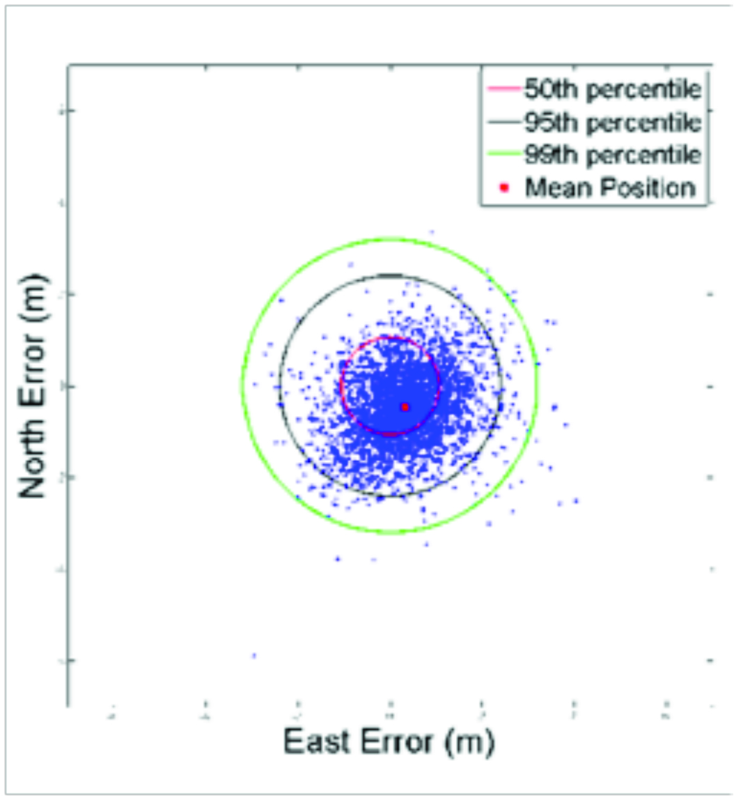
The plots from Figures 3, 4, and 5 show the errors in position estimates obtained from a 24-hour dataset recorded at the HUEG IGS station in Huegelheim, Germany on May 5, 2010. Table 1 shows the statistics associated with the figures.
Figure 3. Stand-alone GPS horizontal positioning performance over 24 hours at HUEG IGS station.Figure 4. Conventional EGNOS horizontal positioning performance over 24 hours at HUEG IGS station.Figure 5. Position domain EGNOS horizontal positioning performance over 24 hours at HUEG IGS station.TABLE 1. Horizontal positioning performance statistics from 24hr HUEG IGS station analysis.
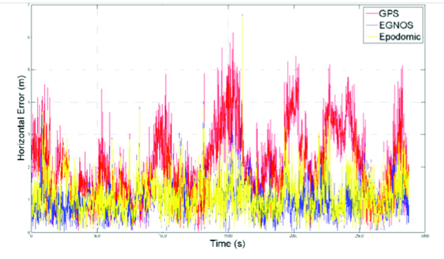
The results demonstrate that the conventional EGNOS solution improves the horizontal positioning performance of GPS, with an improvement in the 95th percentile of around 2 meters in this example. Importantly, it can be seen that the position domain EGNOS algorithm achieves a similar level of performance to conventional EGNOS. This can be seen more clearly by comparing the instantaneous horizontal error over this period from the three alternative solutions, as shown in Figure 6. It is clear that the position-domain EGNOS correction shown in yellow reduces the horizontal error of the GPS solution (red) in a similar way to conventional EGNOS (blue).
Figure 6. Time series of horizontal positioning errors for stand-alone GPS, conventional EGNOS, and position domain EGNOS solutions at HUEG IGS station.
Similar behavior was found in other datasets tested. With the ability of the algorithm to replicate conventional EGNOS performance verified, we assessed the performance when integrated on an HTC Legend phone. The key differences here were the real-time connection to the EGNOS data server and the uncertainty in the assumptions made regarding the chipset positioning algorithm.
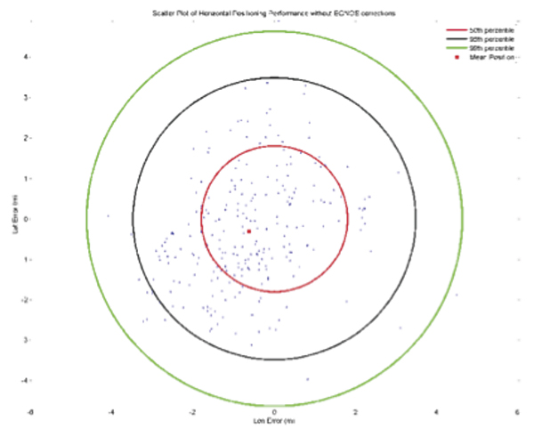
Testing began by assessing the performance of the application over a static point. Two precisely surveyed points were used for this purpose at four separate time periods. The test method simply involved holding the phone over the point (vertical accuracy was not assessed) and requesting a corrected solution from the application, along with the original GPS chipset solution. The chipset applies stand-still detection to avoid generating multiple GPS positions for a single user location which would be unnecessary in typical phone applications. To generate a sample of position estimates therefore the phone was repeatedly moved away from the reference point then returned to it over the test period. This makes the collection of very large datasets over extended periods impractical. The samples from the four test periods were combined in order to generate results with greater statistical significance. 261 samples were collected to produce the results shown in Figures 7 and 8, and the statistics in Table 2.
Figure 7. Stand-Alone GPS Horizontal Positioning Performance from online static point testing.
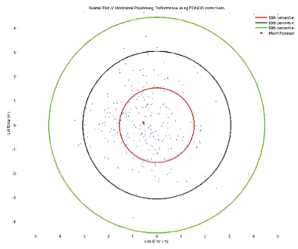
Figure 8. Position Domain EGNOS Horizontal Positioning Performance from online static point testing.TABLE 2. Horizontal Positioning Performance from online static point tests.
The results indicate a small improvement in horizontal accuracy as a result of the position domain EGNOS correction. The statistical significance of these results is perhaps questionable given the limitations of the test method and relative small sample size. The reduced level of improvement compared to the offline tests is thought to be due to imperfect assumptions made about the chipset positioning algorithm. The correction algorithm must make many assumptions about the way in which the original GPS position has been computed by the phone chipset. These include assumptions on the measurement weightings used, an assumption that a filtered solution is not applied, assumptions that no additional sensors or systems (accelerometers, digital compass or cellular positioning) influence the computed position, and also assumptions that all information reported in the NMEA strings is accurate. Further work seeks to determine if the algorithm can be improved to better replicate the processes applied in the initial GPS solution in order to make a more significant improvement.
The phone GPS positioning achieves similar levels of accuracy to processing single-frequency data collected at an IGS station. This level of accuracy would be more than adequate for most LBS applications in which the main requirement is to be able to reliably relate a user location to a map or imagery feature. With increasing solar activity over the next few years, leading to larger ionospheric delays on satellite signals, the performance of standard GPS solutions will degrade, making the benefits of the more accurate and timely EGNOS corrections more significant.
Conclusions and Way Forward
By a relatively simple translation method, EGNOS data may be mapped into the position domain, allowing a user position solution to be corrected for signal-in-space (satellite orbit and clock) and ionospheric errors detected and predicted by EGNOS. User position solution provided by the phone chipset may be corrected in near-real time based on data downloaded from a distant server.
The method replicates conventional EGNOS performance (corrections applied at the pseudorange level) when all assumptions regarding the stand-alone GPS user position are valid. Ongoing work seeks to determine if the correction algorithm can be enhanced to provide a greater level of improvement to GPS positions on the phone platform. Ideally, it should be able to provide improvements similar to those produced when EGNOS data is applied in a conventional manner in the position solution. Developers would need to judge the significance of any potential improvement for their intended application.
The EC has launched a project to port this EGNOS library to other mobile platforms and complement it with additional functions that are needed by the application developers and that can bring user benefits. The software library can be obtained free upon request to [email protected].
Acknowledgments
Special thanks to Nottingham Scientific Ltd. for its work on this topic and cooperation in preparing this paper. This article is based on a paper presented at ION-GNSS 2010.
François Boullete was market development officer at the European GNSS Agency at the time of this work. He holds a diploma in project management from HEC and a diploma in engineering from Ecole Centrale.
Boris Kennes is R&D and market monitoring officer at the European GNSS Agency. He has a background in engineering and strategy consulting.
Michaël Mastier is policy officer at the European Commission in the Galileo/EGNOS applications unit. He has an engineering education and diploma in public works from ENTPE in Lyon, and a computer science post-graduate diploma from Saint-Etienne University, France.
Lee Banfield is a software engineer at Nottingham Scientific Limited (NSL) in the UK. He has developed applications which use EDAS data to provide EGNOS corrections, GNSS assistance messages and GNSS performance metrics for a range of road and LBS applications.
A new method enables the mobile phone to compute its own position using acquisition assistance data with increased resolution in some of the fields. It benefits network operators as they can deliver the best performance with minimum bandwidth requirements, making this especially relevant in emergency-call situations.
By Javier de Salas and Frank van Diggelen
In assisted GPS (A-GPS) and A-GNSS, some information in the form of assistance data is sent to the mobile terminal equipped with a GNSS receiver. This data helps the receiver acquire satellite signals faster and at lower power levels as well as compute its own position. Assistance data is essential in many GNSS use cases but it is especially relevant in emergency calls from mobile terminals (e911, e112) where a fast response and the best sensitivity are required. Mobile subscribers are often in environments where direct satellite visibility is impaired because the user is inside a building or there are other obstructions. Emergency situations also require a very fast response (time-to -first-fix or TTFF), typically within 30 seconds, so the performance requirements imposed on the GNSS receiver are very stringent.
GNSS assistance data is standardized by 3GPP and 3GPP2 in two different types, broadly known as mobile-station (MS) based and MS-assisted. MS-assisted positions are computed by a server. MS-based methods enjoy certain performance benefits in position accuracy and response time when compared with MS-assisted methods. However, the amount of assistance data required for MS-based operation is substantially larger than the assistance data required by MS-assisted methods.
For this reason, some network operators choose the MS-assisted methods for their emergency-call services. Larger bandwidth requirements are of deep concern if many callers demand the services at the same time, because network capacity could be challenged when it is most needed.
This article describes a method that enables the mobile terminal to compute its own position, thus enjoying the benefits outlined above but with the same assistance data as in MS-assisted methods, only with increased resolution in some of the fields. We call this method single-shot MS-based. Network operators benefit because they can deliver the best performance with the minimum bandwidth requirements, especially relevant in emergency call situations.
Some 3GPP specifications will need to be modified slightly to increase the resolution of the relevant assistance data fields, namely, 3GPP TS 44.031, 3GPP TS 25.331, and 3GPP TS 36.355
Bandwidth versus Performance
Assisted GNSS information is exchanged between the location server and the mobile device using standardized protocols. Several bodies create different specifications: 3GPP, 3GPP2, and the Open Mobile Alliance (OMA). Broadly speaking, we can say that 3GPP and 3GPP2 work on protocols that are used over control plane and OMA works on protocols that are used over user plane.
Control plane refers to the use of cellular signaling channels as the transport mechanism for the assistance data and position information. User plane refers to the use of traffic channels (see Figure 1). When you get a phone call, the control plane makes your phone ring. When you browse the web you are using the user plane.
Figure 1. Control plane is used for signaling purposes, user plane for transferring user data.
Signaling channels are not designed to transfer large amount of information, so it is important for 3GPP and 3GPP2 to make the protocols efficient and save bandwidth while maintaining the best performance. Cellular traffic channels are designed to transport much larger amounts of data and thus the bandwidth restrictions are less important than in the control plane case; OMA typically addresses richer GNSS features for Location Based Services (LBS). This is why network operators often support emergency call location using control plane, leaving the user plane for commercial applications. It is also a very good way to separate emergency traffic from LBS traffic so that the former is never compromised by lack of capacity coming from heavy use of commercial location applications.
Two different types of assisted GNSS have been standardized, known as MS-based and MS-assisted in Global System for Mobile Communicatios (GSM) and code-division multiple-access (CDMA) specifications, and as user-equipment (UE) based and UE-assisted in Wideband Code Division Multiple Access (WCDMA) specifications.
MS-assisted refers to the case where the mobile device equipped with a GNSS receiver does not compute its own position but it is instead computed in a location server in the operator’s network. Assistance data is sent to the mobile device to help acquire satellite signals faster. Remember that GNSS signal acquisition involves a three dimensional search (satellite, frequency and delay) that requires intensive signal processing. So assistance data is sent in the form of visible satellites including expected delays and expected Doppler shifts. These values are provided at a reference time and relative to an approximate location for the subscriber. The approximate location typically comes from the location of the serving cell tower. The reference time, but not the approximate location, is normally included as part of the assistance data. After a certain number of satellites are acquired, measurements are sent back to the location server for it to compute the subscriber position. GNSS measurements for each satellite include the measured delay, measured Doppler frequency and an estimation of the signal power to noise ratio. Assistance data in MS-assisted is referred to as “acquisition assistance”. It contains the minimum information so it is very efficient in bandwidth. See Table 1 for an exact bit count of the GNSS acquisition assistance. This table will be used as an example throughout this paper. In this particular example, it is assumed that assistance data is sent for 16 satellites.
MS-based refers to the case where the GNSS-enabled mobile device computes its own position locally. A different set of assistance data parameters are sent to the device to help it acquire the GNSS signals as well as calculate its own geographical location. Measurements are processed by the mobile device internal circuitry until the locally computed position is deemed accurate enough to meet the requirements received in the location request or a timeout is reached. Location information (latitude, longitude, altitude) is then sent back to the network in response to the location request. Assistance data in MS-based consists, at a minimum, of three elements: an approximate location (coming from the serving cell), an approximate time (accurate to a few seconds) and a description of the satellite orbits and clock errors referred to in the specifications as navigation model. See Table 2 for an exact bit count of the GPS assistance data in MS-based. The GNSS receiver uses the approximate location, the approximate time and the navigation model to estimate the expected delays and Doppler shifts of the visible satellite and thus proceed to the acquisition of satellite signals very much like in the MS-assisted case. Satellite measurements (code delays in the simplest implementation) and navigation model are used to calculate the receiver’s own position as explained below.
Advantages of MS-Based over MS-Assisted
We can see from Tables 1 and 2 that the amount of data used in MS-based i
s significantly larger than that of MS-assisted, in fact by a factor of seven! So why do some operators still decide to use MS-based over MS-assisted? The answer is there are noticeable performance advantages when using MS-based. An in-depth description of these advantages is out of the scope of this paper; but we will provide descriptions of what we see as the three more important ones.
Better Estimate of Position Accuracy. The first advantage lies with the fact that in MS-based mode the mobile device has a much better knowledge of the estimated accuracy of the position that it has computed internally. This was implicitly mentioned in the description of the MS-based and MS-assisted method above when we explained that in MS-assisted mode, the mobile terminal sends the measurements after a sufficient number of satellites (with certain range uncertainties) have been acquired. This is precisely the problem, what is a sufficient number of satellites? It is not easy to know for the mobile receiver because it does not know what positioning algorithm or what satellite subset the location server will use in its calculations. As such, it is more difficult to guarantee the quality of service of the position in the MS-assisted method. One could perhaps argue that the mobile receiver has an idea of the satellite geometry based on the Azimuth and Elevation fields (see Table 1) and therefore can perform a more educated estimation than just using the number of satellites and their associated uncertainties. This argument will only be valid if the mobile device knew exactly what the satellite subset is that the location server will employ in its position computation. Different satellite subsets yield different estimated accuracies. In addition to this, azimuth and elevation fields are optional in other positioning protocols such as Radio Resource Location Protocol (RRLP) and Radio Resource Control (RRC) and are also quantized with a value of 11.25 degrees, which deems them practically useless to quantify the satellite geometry in the critical cases where the dilution of precision (DOP) values are large.
Kalman Filter. The second advantage comes from the use of sophisticated navigation filters (for example, Kalman filters) by all GNSS manufacturers. In the MS-based method, the final position estimate that is sent to the network is computed using consecutive sets of measurements that help the position converge using the receiver dynamic model to smooth the resulting positions for greater accuracy. Conversely, in MS-assisted mode, the position computation engine only has access to a single set of measurements and therefore cannot employ sequential navigation filters.
Coarse-Time A-GNSS. The third advantage is perhaps the more difficult to grasp. It has to do with the fact that most (if not all) A-GNSS location servers only provide reference time information that is accurate to within a few seconds. On the other hand, for classical GNSS position computation, knowledge of absolute time accurate to a few milliseconds is required. Typically, it is the task of the GNSS receiver to decode the accurate satellite time information that comes modulated on the GNSS signals as part of the navigation message. However, in environments where satellite visibility is impaired, such as indoors, the satellite signals may be so low that the timing information cannot be decoded from the satellite due to excessive Bit Error Rate. In these situations, the absolute time can be set as an additional state that to be solved as part of the complete navigation solution therefore increasing the position yield in of the GNSS receiver in difficult environments. We refer to this technique as coarse time A-GNSS.
There is no technical reason why this technique could not be implemented in a location server in the operator’s network as opposed to the mobile device itself. However, for this technique to work properly, the mobile device should indicate to the location server whether or not it has successfully decoded the time from the satellites signals (or perhaps other sources). This is normally done by setting an associated time-uncertainty value with the time reported with the GPS measurements. There are some 3GPP specifications (for example RRC prior to R7) that do not support this parameter so they have hindered the adoption of the coarse time A-GNSS technique in MS-assisted mode.
Continuous Navigation. By delivering ephemeris data (good for several hours), MS-based techniques have an advantage over MS-assisted for continuous navigation. This advantage is not addressed further in this article, where we are focused only on first fixes.
Single-Shot MS-Based Method
We present a brief reminder of how GNSS positions are computed in order to determine what assistance data is strictly needed for a mobile terminal to compute its own location. We will use a simple least squares algorithm for simplicity but the conclusions are extensible to the cases of other positioning algorithms such as Kalman filters.
The observation equations are typically linearized around an approximate location. They can be easily presented in matrix form as:
Δ y = A Δ x
where Δ y is a column vector [m x 1] containing the difference between the predicted and measured pseudo-ranges for the m satellites measured by the GNSS receiver. The predicted pseudo-ranges can be obtained using the acquisition assistance data (codePhase and intCodePhase fields.)
Δ x is a column vector [4 x 1] containing the change in the “state” from the approximate position. The state has four unknowns x, y, z and b. x, y, and z are the change in the local East (longitude axis), North (latitude axis) and Up (altitude axis) coordinates from the reference position, b is the common mode error (mostly from the internal receiver clock error) in distance units.
A is an [m x 4] matrix, the first three elements in each row ux , uy , uz are the coordinates of the unit vectors from the receiver to the satellite, the last element is a 1 for the common mode error. A is sometimes referred as the geometry matrix.
Coordinates of unit vectors can be written as a function of the azimuth and elevation of each satellite. Simple trigonometry yields:
ux = cos (el) * sin (az)
uy = cos (el) * cos(az)
uz = sin(el)
In the coarse-time case there will be a fifth column of A containing the range rates, which are provided in the MS assistance data.
The goal is, of course, to determine the change in the state (our unknowns). Using simple least squares
Δ x = (ATA)–1AT Δ y
we can easily determine Δx. The coordinate changes in Δx (delta position) will be applied to the approximate location to obtain the new position.
Assistance Data Required
To re-cap from the previous section, we have seen that to compute Δx we need:
Expected pseudo-ranges for satellites in view (from acquisition assistance)
Measured pseudo-ranges (from the GNSS receiver)
Azimuths and Elevations for the geometry matrix (from acquisition assistance)
It would seem that if the mobile device receives acquisition assistance and measures the pseudo-ranges for a few satellites, it has everything that is required to compute a position (or at least a delta position) inside the GNSS mobile device. The delta position is relative to the position used to compu
te the acquisition assistance. Have we achieved our goal of computing position inside the mobile device with acquisition assistance? Not quite. Let’s now look at the acquisition assistance data in more detail.
We explained that we obtain the required expected pseudo-ranges from the acquisition assistance fields codePhase and intCodePhase. The codePhase field is defined with a resolution of one GPS chip, equivalent to 300 meters. Recall that we subtract the expected pseudo-range from the measured pseudo-range before we use the measurements in the position solution so this means if our expected pseudo-range was in error by, say, 150 meters because of the low resolution of this field, this is similar to making a measurement error of that amount, which of course will cause an unacceptable position error. This means the resolution of the codePhase field would need to be increased to be able to compute position. For a resolution of 2 meters, 8 more bits would need to be added.
The second topic of interest relates to the azimuth and elevation fields. These are needed to construct the geometry matrix A. As mentioned before, in 3GPP location protocols the azimuth and elevation of the acquisition assistance element are defined with a resolution of 11.25 degrees. Sines and cosines (needed to calculate the coordinates of the unit vectors) with such large angle errors will also yield large position errors. In Long-term Evolution Positioning Protocol (LPP), the situation has improved with the resolution being 0.7 degrees.
In an effort to quantify how the angle quantization affects the position error, we have run simulations that plot the 95 percentile of the HDOP error as a function of the angle error in azimuth and elevation (see Figure 2.) HDOP is proportional to the position error so this seems to be a reasonable choice. N is the number of satellites used in the simulations. As you might expect: the fewer the satellites the greater the effect.
Figure 2. HDOP error vs Az/El error. We use HDOP as a proxy for the expected position error: if the HDOP changes by 10 percent, we expect the position error to change by a similar amount.
We can see from the plot in Figure 2 that for an angle resolution of 0.7 degrees as currently defined in LPP, the 95 percent HDOP error is under 12 percent. If we wanted to make the worst error (N=4) under 2 percent, we can see that the resolution should be increased to 0.1 degrees. In order to meet this goal, 3 more bits would need to be added to both the azimuth and elevation fields in the acquisition assistance.
Another effect that must be noted is the possible change in the azimuth and elevation from the time the assistance data is received to the time the receiver computes its position (or delta position). In an emergency call scenario, typically we assume this time will not be greater than 24 seconds. Note the total allowed response time for an E-911 call is 30 seconds, including call establishment and network latencies. Simulations based on satellite geometry show that the worst-case effect is approximately of the same order of magnitude as the angle resolution discussed above, and therefore its impact in HDOP is just a few percentage points in the case of N=4.
At this point we seem to have everything we need to compute positions (or delta positions) inside the mobile terminal with the same acquisition assistance used in MS-assisted; albeit with slightly higher resolution in some of the fields.
To facilitate the comparison with MS-assisted and MS-based methods, Table 3 summarizes the exact bit count needed for Single Shot MS-based.
Optionally, if an absolute position is required in the mobile device instead of delta position, it would also require the approximate position (reference location) to be sent along with the rest of the assistance data (acquisition assistance, reference time). However, the MS-based performance advantages listed above can all be realized without the reference location, using only delta position. This is why we have not included Reference Location as an element that is needed for Single Shot MS-based.
Conclusions
We have seen that Single Shot MS-based can be used to enable all the MS-based performance advantages with, essentially, the same assistance data that is used in MS-assisted. Minimal additional bandwidth is required due to the increased resolution of some of the fields. Single Shot MS-based is therefore the best option for network operators that deploy A-GNSS based emergency location.
Not only does MS-based require significantly more bandwidth than MS-assisted (~ 7x) or Single Shot MS-based (~ 6x); but the absolute difference will increase with additional GNSS satellites such as GLONASS, SBAS, QZSS, Compass, and Galileo. Imagine all navigation models have to be sent for all satellites in view and for all GNSS constellations! Acquisition assistance can easily be made generic for every GNSS constellation since it is just “range and Doppler” and, in fact, this is the way it has been conceived in LPP where the dynamic ranges for all parameters are no longer restricted to GPS but allow other GNSS constellations.
Javier de Salas is director of GPS product marketing at Broadcom. Previously he worked at Ashtech, Magellan, and Global Locate. He has an MS in electrical engineering from Universidad Politecnica de Madrid.
Frank van Diggelen is chief navigation officer and senior technical director for GNSS at Broadcom. He is also a consulting assistant professor at Stanford University and is the author of A-GPS: Assisted GPS, GNSS and SBAS. He holds more than fifty issued U.S. patents on A-GPS and has a Ph.D. in electrical engineering from Cambridge University.
Inexpensive, readily available GPS jammers constitute a threat to safety, national infrastructure, and industry revenue streams. Cell phones could incorporate GPS jam-to-noise (J/N) ratio detectors to provide timely interference detection and effective localization, with a flexible and updateable system since the crowd processing function resides in software.
Events in early 2010 at Newark Liberty International Airport demonstrate the vulnerability of civil GPS infrastructure to interference. Over a period of several weeks, sporadic outages of the GPS Ground Based Augmentation System (GBAS) located at the airport to provide precision approach services occurred, due to radio-frequency (RF) interference from unknown sources. Analysis showed that certain vehicles on a nearby freeway were the likely culprit(s), and an interdiction effort was launched to catch an offender. Using advanced interference detection equipment and multiple surveillance cameras, an offender — a truck driver — was caught and arrested. In his possession: a widely available $33 GPS jammer.
For sale over the Internet, the jammer emits 200 mW and plugs directly into a vehicle’s cigarette lighter (see photo). To prevent future incidents, the FAA is relocating the airport’s GBAS system to a more protected location away from the freeway.
Such an approach to jammer detection, localization, and enforcement, while successful in this instance, ultimately serves only as a stopgap. It took tremendous resources and several weeks to find one offender.
Increasing use of GPS jamming and spoofing to cover both licit and illicit activities is likely, given the general public’s desire for privacy and the general lack of awareness of how devastating GPS jamming can be. The $33 jammer in this instance could have affected critical flight operations 10 miles away. Currently, most jammers are not even detected; we simply have an unidentified GPS outage. It was only because of the technical sophistication of the FAA’s GBAS that the outage’s underlying cause was identified as jamming.
GPS Jammer. A $33, 200mW jammer for sale over the Internet.
At the ION-GNSS 2010 plenary session, Phil Ward advanced the notion that cell phones could incorporate GPS jam-to-noise (J/N) ratio detectors to provide timely interference detection. Having an extensive background in cellular communications as well as GPS, I found the idea intriguing. In this article, I explore the viability of this concept, whether jammer location can be determined, and what it would take to implement such a system.
In urban and suburban areas, it appears feasible to provide warning of jamming in less than 10 seconds while providing real-time jammer location to better than 40 meters. Such a capability would aid immensely in mitigating jamming events by enabling effective law-enforcement action. Potential jammers will know they are likely to be caught and that the penalties are severe. They won’t do it after a few well publicized interdictions. The cost for this nationwide system can be relatively modest. It won’t take billions of dollars and decades to implement; it will take an act of national will similar to the phase II wireless E911 effort. IOC could happen as early as 2015, with full national coverage by 2017.
J911 System Architecture
Figure 1 depicts the automatic gain control (AGC, the process by which RF front-end gain is controlled so as to present the analog-to-digital (A/D) converter with appropriate signal levels) loop found in some form in virtually all GPS receivers. The core objective is to set the gain GA so a set percentage of 2-bit A/D converter outputs correspond to large values of 3 and -3. Typically, VT percentage is set to 35 percent in a Gaussian noise environment to hold A/D conversion losses to ~0.5 dB. In another popular variation, the 1.5 bit A/D converter, the zero threshold is not implemented and three possible values are output (-1, 0, and -1). Such a converter has about 0.9 dB of conversion loss if VT percentage is set to 40 percent, and considerably simplifies correlator processing.
Figure 1. Adaptive A/D converter with jamming-to-noise (J/N) meter output. Knowing you are jammed is the first step.
Figure 2. J/N as a function of position relative to a 200 mW jammer. phones located closer to the jamming source will see higher J/N than those further away.
Of particular interest for interference detection purposes, the control voltage to the AGC amplifier can also be used to measure jammer-to-noise power (J/N). Under unjammed onditions, the nominal input power to an L1 C/A receiver is about -110 dBm, most of this due to naturally occurring thermal and amplifier noise. The C/A code signal at -130 dBm is a factor of 100 weaker and does not influence AGC operation. If, however, interference starts rising above the thermal noise floor, the AGC will respond by decreasing gain GA so as to maintain the correct percentage in large outputs. Response times to a change in input power level are very fast, typically less than 1 millisecond, and so pulse jamming characteristics can be determined as well.
If the receiver knows the control characteristics of the AGC amplifier (β,α) then the receiver can determine the change in J/N given V1. Additionally, if the receiver knows the quiescent V1 associated with a thermal noise-only input, it can obtain J/N on an absolute scale. To obtain the quiescent value, the receiver can short the antenna on power-up as part of built-in test prior to operation. Alternatively, it can maintain and refine a historical value during normal operations, the caution being that spoofers and jammers may try to manipulate history-based values.
Even with relatively small jammers, front-end saturation can be a problem when the jammer is nearby. The thermal noise floor in a 1.7 MHz bandwidth is about -110 dBm, and so a J/N of 60 dB corresponds to jamming signal strength of -50 dBm. Accurate J/N measurements are possible at this level, but likely require adding a switchable input step attenuator in the down-conversion chain. Measuring J/N above this level gets problematic for a low-cost GPS front-end.
In a further refinement, receivers can include additional comparators set at -1.2 VB and + 1.2 VB. If a constant envelope (CE) jammer (CW, swept CW, or Gold code jammer types) is present, this threshold will be crossed 16 percent of the time given CE jamming, versus 32 percent of the time for Gaussian distributed jamming if VT percentage is set to 40 percent, as is typical for a 1.5 A/D converter. With the jammer type identified, the receiver can adapt V<su
b>T percentage if it is seeing CE jamming to obtain several dB of additional jamming resistance. The TI-420 L1 C/A receiver developed by my team at Texas Instruments in 1986 routinely outperformed P-code receivers against CE jammers using this technique. The takeaway from this discussion is that with very simple hardware, an L1 C/A receiver can measure J/N and also determine the approximate type of jamming that it sees: pulse, constant envelope, and Gaussian.
Can this information be used to detect and locate jammers? In Figure 2, a 200 mW jammer is located at the origin [0,0] and J/N (dB) is plotted as a function of relative location. Conceptually, phones located closer to the jamming source will see higher J/N than those further away. The aggregate of phones, each reporting J/N and own position, provides a basis for locating the jammer. Some phones may also report the type of jammer they are seeing. Information about phone type and its physical orientation would also be of use in interpreting and correcting raw J/N information with regards to antenna gain and accuracy.
Structurally, the J911 system would be very similar to the E911 system and would heavily leverage existing infrastructure and standards already in place. When a wireless E911 call is placed, the serving base-station(s) routes the call through a mobile switching center (MSC) where the call is identified as a 911 call. The MSC then connects the call to a local exchange carrier (LEC) who then connects the call to a public safety answering point (PSAP).
In the United States, 6,149 PSAPs are distributed around the country.Wireless E911 calls are connected to a specific PSAP usually based on the location of the caller as determined by the cellular carrier. Under Phase II requirements, E911 call takers receive both the caller’s wireless phone number and their location information. Currently, 95 percent of PSAPs have some Phase II E911 capability.
Using the E911 system as a basis, creating a federal J911 PSAP to process J/N measurements into jammer location estimates would not be all that problematic. Software upgrades to phones, base stations, MSCs, and so on, are routine and often include new or modified message provisions and capabilities. Adding a Jamming Report message type would use existing message transport and routing facilities already part of the infrastructure. The main infrastructure addition would be a facility to process jamming reports, either at the federal level or as an adjunct to existing PSAPs.
Adding a J/N measurement capability to phones is a straightforward hardware issue, but modifying extant phones is not feasible. Fortunately, cell phones typically have a two-year lifecycle before being replaced. Adding a jammer reporting capability can be accommodated through the normal replacement cycle.
J911 System Performance
Given the location and J/N measurements obtained by a crowd of randomly located cell phones, one approach to determining the jammer’s location is to perform a series of curve fits for a grid of hypothetical jammer locations and see which location provides the best fit. Figure 3 illustrates this process; for the moment, the cell phones (observers) are assumed to provide exact J/N and location measurements.
Here, a 200 mWatt jammer is located at xy = [0,0]. 1,000 cell phones are uniformly distributed over a surrounding 1-square-kilometer area. A hypothetical jammer location grid of points 5 meters apart is created over a span of ±150 meters in x and y. At each hypothetical point, the 250 highest non-saturated J/N reports are used in a least-squares curve fitting process that assumes jamming strength falls off as 1/Rα. (In the ground mobile environment, α is usually in the range of 2 to 4. α = 2 is consistent with a free space propagation model.)
Specifically, J/N (dB) is presumed to be a linear function of log10 (R) where R is the range from reported observer position to hypothetical jammer location. At each hypothetical jammer location point, the norm of the residuals is collected as a metric of how closely the jamming reports (J/N + location) matched the least squares curve fit. The smaller the norm of the residuals, the better the curve fit. This metric is plotted in Figure 3 and shows that the best fit is obtained at the true jammer location.
Figure 3. Location metric as a function position relative to true jammer position (no observer errors).
In practice, knowledge of cell-phone locations is imperfect, and for those phones near to the jammer, GPS will be unavailable. There are several alternatives for determining location. Cellular carriers use a plethora of location determination techniques based on round-trip timing between the cell phone and observing base stations. Another very good option is to use Wi-Fi-derived location based on visible access points (AP). Companies such as Skyhook and Google have commercialized this technology, and it is available now in most areas. Positioning accuracies of 30 meters are typical, absent GPS. Looking down the road a bit, many phones now have integral accelerometers and could in the future propagate position with good accuracy even when GPS is unavailable.
Another very important factor is that J/N observations are going to be highly variable.
Three major effects to consider:
Cell phone errors in measuring J/N due to quiescent V1 errors, imperfect AGC amplifier characterization, and uncompensated receive antenna gain directionality.
Variability in J/N due to large-scale shadowing due to buildings, hills, bridges, etc.
Variability in J/N due to small-scale multipath effects. Jamming signals may follow multiple paths to the cell phone and add up constructively or destructively. Moving the cell phone a few inches may yield a very different J/N.
To model these effects, a log normal model of J/N measurement deviation from ideal free-space propagation is used. In this model, free-space propagation represents median signal strength and σ log normal, expressed in dB, describes Gaussian random deviation from the median signal strength. Such models are widely used in predicting statistical cellular coverage and have a strong correlation with real-world observations.
Figure 4 shows a jammer location metric manifold computed using the same process as in Figure 3, except now with observer location errors of
σx = σy = 30 meters and σ log normal = 6dB. Basically this says that the cell phones have Wi-Fi-based locations, and that the measured J/N is within ±6 dB of the free space value 68 percent of the time, and, within ±12 dB of the free-space value 95 percent of the time. These are relatively modest performance goals for the cell phones.
Figure 4. Location metric as a function position relative to true jammer position (observer errors: 30 meter 1 /6 dB 1 J/N).
In this particular run, the hypothetical jammer position yielding smallest residual norm is at xyjammer = [10,45] meters. Even though the individual measurements are of poor quality, the crowd consensus yields a fairly accurate estimate of the jammer’s position.
Before continuing, a few words on crowd size and cell phone densities. Assuming a cellular penetration rate of 70 percent, Table 1 shows approximate cell-phone densities for select suburban and urban municipalities. No doubt there is considerable variation in cell phone densities even within a municipality, but as a rough order of magnitude, 1,000 cell phones per square kilometer is not an unreasonable number.
Table 1. Density of 1,000 phones/square kilometer Is common in urban areas.
Figure 5 shows statistics of jammer location accuracies, presuming a uniformly distributed cell phone density of 1,000 cell phones per square kilometer. Based on a simulation of 500 independent runs, this figure plots jammer location radial error statistics assuming 25, 100, 500, or 1,000 measurements are processed in the curve-fitting process where radial error is given by:
Processing the full crowd yields 14-meter or better radial errors in 50 percent of the trials and better than 27 meters in 90 percent of the trials. So why process less than the full set of measurements obtained by the cell phones? In practice, if all cell phones observing a jamming event were to report everything they see, the cellular infrastructure could be overwhelmed. To limit traffic surges and to limit false alarms, a jamming event is likely to be processed in two distinct phases; the detection phase and the locating phase.
Figure 5. Radial error statistics with 1,000 phones/sq km crowd density.
Jammer Detection
In the detection phase, cell phones would report relatively infrequently based on which page group they are in. In current practice, to minimize cell-phone power consumption while in standby, each cell phone belongs to a particular page group based on its supposedly unique International Mobile Equipment Identity or IMEI. (As a bit of trivia, most cell phones display their IMSE if you dial *#06#). In GSM there may be 50 distinct page groups. Depending on which page group the phone belongs to, the phone knows when to wake up to listen to the paging channel (PCH) and see if there is an incoming call for it. By limiting jammer reporting based on which page group the phone is a member of (or IMEI), the size of the initial traffic surge can be limited.
During the detection phase, the system will also need to determine the type of interference event being seen. A solar event may trigger large numbers of phones, but the flat J/N versus location response can be used to rule out a localized jamming event. A real jamming event will tend to have a geographic center with many high J/N values over a fairly restricted area. Also, if CE interference is reported as opposed to Gaussian interference, there is good confidence the event is human originated, and the source can be located.
Jammer Localization
If jamming is determined to be the cause of interference, then the system transitions to a jammer localization phase. Tentatively, the jammer location process would seem to be better served by using phones near the jammer, but not those phones with saturated J/N meters. The non-saturated phones provide good RSSI (received signal strength indicator) information that is correlatable with distance, and those cell phones closest to the jamming source (high J/N) tend to experience fewer propagation anomalies. To control traffic loads during a jamming event, the J911 PSAP may restrict which phones report by requesting that only phones seeing a J/N value of greater than J/Nmin report.
Returning to Figure 5, processing the full set of data yields better snapshot jammer location accuracy as opposed to results obtained using a trimmed subset. Processing the full crowd yields 14 meter or better radial errors in 50 percent of the trials and better than 27 meters in 90 percent of the trials. Relying on only the subset of the 250 strongest J/N values adversely affects jammer snapshot location accuracy; yielding 47 meter or better radial errors in 50 percent of the trials and better than 110 meters in 90 percent of the trials.
The upside is that the traffic generated on the cellular network is one quarter as much. Stated another way, for a given traffic handling capacity, we could update jammer location at four times the rate. Using page group membership, general location, or IMEI as an additional reporting criteria, we can sample different cell-phone populations at each snapshot interval.
If a Kalman filtering approach is used to track/smooth jammer location estimates, the reduced set of observations may ultimately yield better performance, especially considering that individual phones can move around considerably over time. Also, geographical centroiding using phones with saturated or very high J/N indications may be another viable jammer locating technique, and perhaps combining approaches would be good. If the jammer is determined to be in a vehicle, substantial accuracy improvements in location accuracy may also be obtained by limiting the hypothetical jammer location grid to include only roads based on map input. These are all open issues for further study.
Figure 6 repeats the analysis of figure 5 except now, cases of much reduced cell-phone density are considered. In all cases, the full set of data is reported and processed. Not surprisingly, with more observers, the jammer locating accuracy is better, but even with low cell-phone densities, the performance is not bad: 50 meters 50 percent of the time, and 100 meters 90 percent of the time with 100 phones per square kilometer. Jamming detection and location is feasible in modestly populated areas.
Figure 6. Radial error statistics with crowd densities of 50, 100, 250 and 1,000 phones per square kilometer
Figure 7 shows radial accuracy statistics for σlognormal = 4, 6, 8 and 10 dB. As expected, as J/N measurement reliability deteriorates due to increased propagation variability and/or cell phone measurement errors, the accuracy of jammer location estimates also deteriorates but not catastrophically so.
Figure 7. Radial error statistics with σlog_normal =[4,6, 8, 10] dB crowd densities of 1,000 phones per square kilometer.
Similarly, simulation runs with larger cell-phone location errors showed modest performance losses in jammer location accuracy. In aggregate, Figures 5 through 7 point towards crowd size and crowd selection algorithm, not the accuracies of individual measurements, as the main driving factors in jammer-location accuracy.
Putting J911 in Place
Initially, wireless operators had little enthusiasm for implementing wireless E911 as it introduced substantial hardware requirements for mobile station (MS) position reporting (a cell phone is an MS). Now, E911 provides the technical underpinning for numerous revenue streams, most notably the location-based services (LBS) industry. GPS jamming is a direct threat to this revenue stream.
As GPS becomes integrated with vehicle navigation systems and intelligent highway systems, cellular carriers will play an important role in provisioning needed communications facilities. GPS jamming is a direct threat to this future revenue stream.
Cellular signal jamming is also a threat to national infrastructure (and carrier revenue). The approaches described above are readily adaptable to detecting and locating cellular frequency band interference sources in a timely manner. By emphasizing the potential benefits of a J911 system to the cellular carriers, there is better potential for buy-in by industry.
Using the wireless E911 experience as a model, J911 could be made a reality using a three-step process:
Rulemaking. After validating the requirement, the FCC would issue a Notice of Proposed Rulemaking (NPRM) stating the system functional requirements. Industry would comment, and through an iterative process the J911 requirements regarding performance and mandated deployment schedules would be established. This process would take about two years.
Standards Setting. Well established wireless, LEC, and PSAP standard-setting bodies would create detailed standards for implementing J911. The bulk of the work would be done by collaborating representatives from industry. Standards would be issued for various system portions — for example, MS standards, BSS standards, and so on — to permit manufacturers to build interoperable equipment. The standards setting process would take one to two years.
Rollout. With the exception of the MS portions, J911 does not require hardware modifications to the cellular infrastructure. J911 would be implemented and deployed as part of the normal update and release cycle. Under the mandate, new mobile stations would have to meet the requirements of the FCC rulemaking and standards setting processes. Over a two-year period, mobiles would transition to J911 capable models and the J911 system would be in place.
Crowdsourcing
In the March 7, 1907, issue of Nature, Francis Galton reports on an experiment where, at a county fair, he had 787 people guess the dressed weight of a fatted ox, charging them six-penny a guess. Individual estimates varied wildly, as did the expertise of the guessers. However, the median estimate of the crowd was within 0.8 percent of the correct value.
Conclusions
Creating a national infrastructure for detecting and locating GPS and cellular jammers is needed. Such a capability would provide the underpinnings for rapid and effective enforcement actions. Crowdsourcing approaches using a multitude of opportunistic cell phone based observers appears a plausible solution providing timely and location specific alerts. Even though the individual measurements are of poor accuracy, the crowd consensus yields good accuracy. While this system would not reliably detect purpose-built precision power-controlled spoofers, it could detect coarser cell-phone apps-style spoofers that might, for example, be seen in road-use tax avoidance.
Numerous open issues remain. Jammer antenna gain patterns can adversely affect locating accuracy. To what extent can this be mitigated by mapping out antenna gain contours? How can multiple simultaneous jammers be resolved? Can map and propagation modeling based aiding algorithms improve jammer location accuracy?
Significant research is needed, but the proposed system is open for continual improvement, even after it is fielded, since the crowd processing function resides in software.
Logan Scott is a consultant specializing in radio frequency signal processing and waveform design for communications, navigation, radar, and emitter location. He has more than 32 years of military and civil GPS systems engineering experience. As a senior member of the technical staff at Texas Instruments, he pioneered approaches for building high-performance, jamming-resistant digital receivers. He is currently active in location-based encryption and authentication, high performance/low bias adaptive array technologies, and RFID applications. He teaches Navtech Seminars’ New Signals course and holds 32 U.S. patents.