Author: Richard B. Langley

  • Innovation: Self-driving cars in urban neighborhoods

    Innovation: Self-driving cars in urban neighborhoods

    Photo: chuyu/iStock/Getty Images Plus/Getty Images
    Photo: chuyu/ iStock/Getty Images Plus/Getty Images

    How inertial systems and GNSS availability will help

    By Kana Nagai, Matthew Spenko, Ron Henderson and Boris Pervan

    Self-driving cars in urban environments can be problematic. The required multi-sensor automated systems will include GNSS, but buildings block and reflect GNSS signals, reducing system availability and accuracy. Researchers from the Illinois Institute of Technology report on how inertial navigation systems coupled with wheel-speed sensors and vehicle dynamic constraints can help.


    Innovation Insights with Richard Langley
    Innovation Insights with Richard Langley

    ARE WE THERE YET? This was a familiar refrain from the backseats of parents’ cars when traveling to a holiday destination or to grandparents when I was growing up. We didn’t have videos on a display attached to the seats in front of us or (who could imagine?) our own personal communication device on which we could call up games, movies or social media channels.

    But I’m not talking about that complaint from our childhoods. I’m asking if we have arrived at the era of the self-driving car. The answer is yes and no. It all depends on what you mean by “self-driving.” We reviewed some of the technologies needed for self-driving or autonomous vehicles in this column in June 2019. And we indicated in the introduction to that column that vehicle autonomy has several levels. SAE International, formerly known as the Society of Automotive Engineers, has defined six levels of autonomy that can be briefly described as Level 0 – no automation; Level 1 – hands on/shared control; Level 2 – hands off; Level 3 – eyes off; Level 4 – mind off; and Level 5 – steering wheel optional.

    Already, Level 1 automation is widely available in modern cars with adaptive cruise control, parking assistance, lane-keeping assistance and automatic emergency braking among the features being offered.

    Level 2 automation, where the automated system takes full control of the vehicle’s acceleration, braking and steering, is available in some production models, although the “hands-off” designation is not to be taken literally — most motor vehicle laws require drivers to keep their hands on the steering wheel.

    Between Level 2 and Level 3, we have conditional automation — the car can drive itself, but the driver must stay alert and be prepared to take over immediately.

    Level 3 is high automation, where a computer fully drives the car at certain times on certain routes such as a highway; while the driver can perform other tasks such as reading a book, they must be prepared to take over operation of the vehicle within a few seconds if alerted by the automated system. While test campaigns are still ongoing, some jurisdictions permit Level 3 operation by ordinary drivers on some roads, and customers will soon be able to buy vehicles with this level of automation. Widespread use of

    Level 4 and Level 5 automation is further off (some would say quite a way off) and remains in development. But famously, last year, Toyota operated Level 4 self-driving shuttle vehicles around the Tokyo 2020 Olympic Village.

    A lot more work needs to be done before we will have arrived at the era of the fully self-driving car that will be able to travel on any road, anywhere in the world, all year around, in all weather conditions. In particular, self-driving cars in urban environments (as opposed to highway driving) can be problematic.

    The required multi-sensor automated systems will include GNSS, but buildings block and reflect GNSS signals, reducing system availability and accuracy. In “Innovation” this month, researchers from the Illinois Institute of Technology report on how inertial navigation systems coupled with wheel-speed sensors and vehicle dynamic constraints can help.


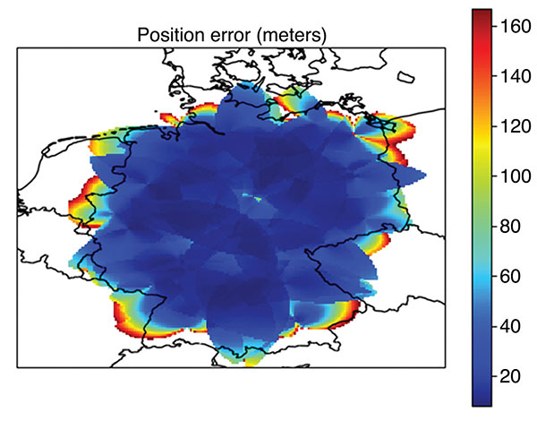
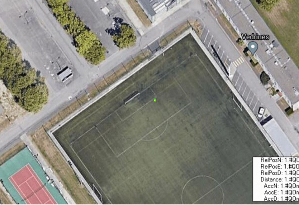
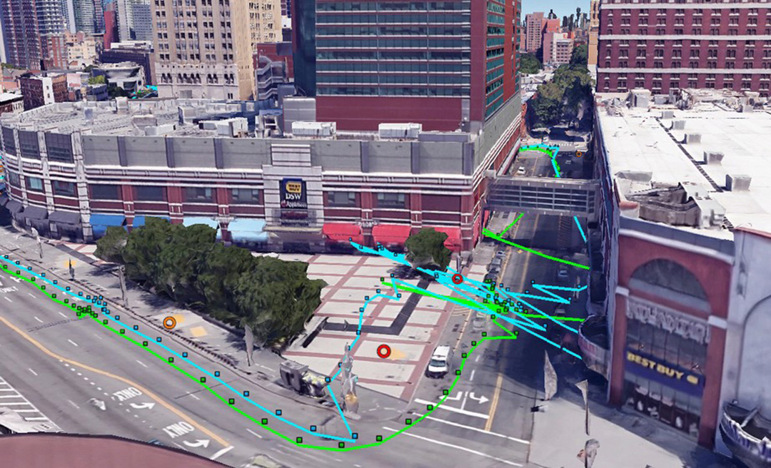
    GNSS provides navigation services globally, but satellite visibility in urban areas is limited by high-rise buildings. This creates a mixture of GNSS available and denied environments (see FIGURE 1) — users do not generally know where the system can maintain sufficient levels of accuracy and integrity for a particular application. To begin to address the issue for self-driving cars, we evaluated GNSS-only availability in downtown Chicago.

    FIGURE 1. The figure depicts three types of potential GNSS signal reception: direct LOS signals and blocked LOS signals (left) and reflected LOS signals (right). (Image: Authors)
    FIGURE 1. The figure depicts three types of potential GNSS signal reception: direct LOS signals and blocked LOS signals (left) and reflected LOS signals (right). (Image: Authors)

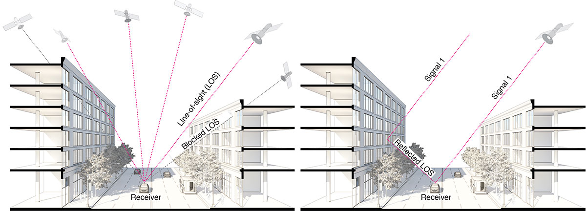
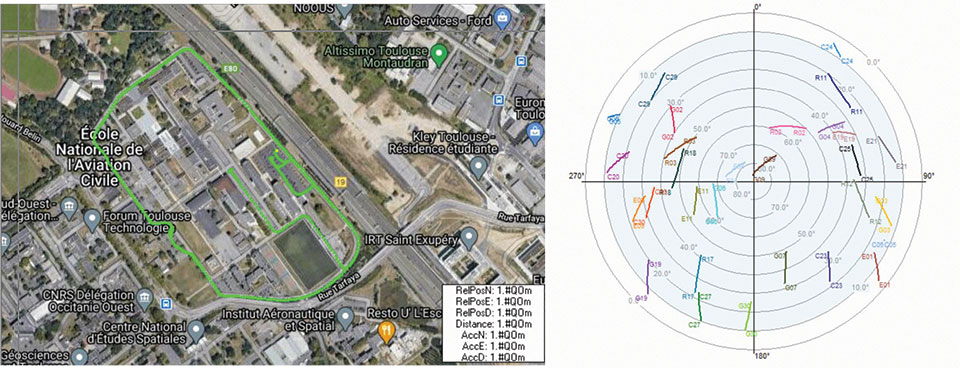
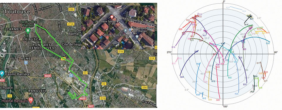
    GNSS signal prediction in urban environments has been conducted in previous work. For example, the concept of “shadow matching” was developed to identify GNSS signal blockages in urban canyons. Overlaying sky plots on a hemispherical sky view can be used to distinguish between line-of-sight (LOS) and non-line-of-sight (NLOS) signals (see FIGURE 2a). Reflected rays can be predicted using Householder transformations to reveal potential multipath conditions. Satellites producing blocked or reflected (NLOS) signals should be excluded to maintain integrity.

    FIGURE 2. (a) A hemispherical sky view in an urban environment. (b) Illustration of a protection level and an alert limit. To ensure integrity, the protection level must not exceed an alert limit. (c) The allowable probability of exceedance is assumed to be 10−7 in this work. (Image: Authors)
    FIGURE 2. (a) A hemispherical sky view in an urban environment. (b) Illustration of a protection level and an alert limit. To ensure integrity, the protection level must not exceed an alert limit. (c) The allowable probability of exceedance is assumed to be 10−7 in this work. (Image: Authors)

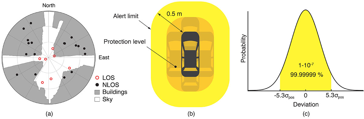
    When the number of visible satellites is greater than three, GNSS can resolve vehicle position. However, even in cases where enough satellites are visible, the satellite geometries are generally weak because the dilution of precision (DOP) is adversely affected by the buildings partially blocking the sky. Horizontal positioning error must be bounded by a protection level computed by the vehicle. Then, for navigation to be deemed available, the protection level must not exceed a required alert limit (see FIGURE 2b). The maximum allowed probability of exceedance (see FIGURE 2c) and the alert limit can together be used to determine the maximum allowable position error standard deviation.

    Even if the protection level is far below the alert limit in an open-sky environment, it will frequently exceed the alert limit once the vehicle enters a city. GNSS alone is generally not able to maintain availability, so integration with other sensors is needed. Tightly coupling inertial navigation systems (INS) with GNSS using the extended Kalman filter (EKF) provides better estimation in urban environments. The EKF algorithm also enables integration of wheel-speed sensors and vehicle dynamic constraints. These integrated navigation systems will improve availability, but it is still unclear how long such a system can be expected to maintain fault-free integrity in a congested city.

    Focusing on the problem of self-driving cars in urban environments, we evaluate protection levels of navigation with practical integrated sensors: GNSS, INS, a wheel-speed sensor (WSS) and vehicle dynamic constraints (VDC). The goal is to develop the means by which we can determine locations where external ranging sources (such as lidar) are needed to maintain continuous navigation with fault-free integrity.

    GNSS-ONLY AVAILABILITY

    For GNSS availability evaluation, we assume an integrity requirement that the probability of exceeding a 0.5-meter alert limit must be lower than 10−7. The 0.5-meter alert limit therefore corresponds to approximately five times the position standard deviation, so the maximum allowable position error standard deviation is then approximately 0.1 meters. Accuracy at this level clearly requires differential GNSS carrier-phase measurements. We assume a nominal GNSS double difference (DD) carrier ranging error standard deviation of approximately 0.02 meters, and that carrier cycle ambiguities can be readily resolved in an open-sky environment prior to initiation of vehicle motion.

    Given the assumptions made of the maximum allowable position error standard deviation and the GNSS ranging error standard deviation, the maximum allowable horizontal dilution of precision (HDOP) is about 5.

    FIGURE 3 shows GPS and GNSS availability — the fraction of time the HDOP requirement is met over 24 hours — along a section of State Street in downtown Chicago. The availability results using GPS only and excluding only blocked LOS signals ranged from 0% to 9% along the block and 9% to 30% at the intersections (see FIGURE 3a). Using four full GNSS constellations (GPS, Galileo, GLONASS and BeiDou), availability ranged from 48% to 82% along the block and 72% to 100% at the intersections (see FIGURE 3b).

    FIGURE 3. The percentage of GPS or GNSS availability in 3D-mapped downtown Chicago. We exclude satellites producing blocked LOS signals or both blocked and reflected LOS (NLOS) signals from the measurements. Each column expresses a lane of southbound or northbound travel. The availability is the percentage of total time when HDOP meets the self-driving car integrity requirements in 24 hours. (Image: Authors)
    FIGURE 3. The percentage of GPS or GNSS availability in 3D-mapped downtown Chicago. We exclude satellites producing blocked LOS signals or both blocked and reflected LOS (NLOS) signals from the measurements. Each column expresses a lane of southbound or northbound travel. The availability is the percentage of total time when HDOP meets the self-driving car integrity requirements in 24 hours. (Image: Authors)

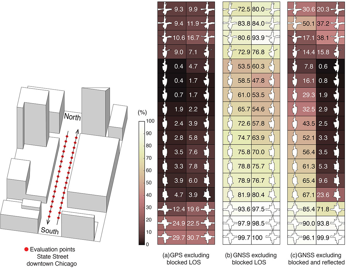
    When we also excluded satellites producing reflected LOS signals that reach the vehicle, the availability dropped significantly at every point (see FIGURE 3c). We assert that FIGURE 3c expresses the reality of GNSS availability because building-reflected multipath signals degrade positioning accuracy and would affect integrity negatively. It’s obvious from these results that GNSS alone is insufficient to meet the autonomous driving requirements in an urban environment, and multi-sensor integrated navigation systems are needed to augment poor GNSS signal availability.

    MULTI-SENSOR INTEGRATION

    We begin by considering tightly coupled INS/GNSS integration using an EKF, and then integrate a realistic sensor suite including WSS and vehicle dynamic constraints that enforce resistance to lateral sliding and vertical movement. If it is known from another source that the vehicle is not moving (for example, it is in the parking gear), a static mode constraint (SMC) can also be applied.

    INS/GNSS Integration. Tightly coupled INS/GNSS integration with an EKF uses the INS measurement to predict vehicle motion. The continuous process model uses a state vector having the position in the navigation frame, the velocity, the attitude, bias errors and cycle ambiguities, with the input vector having accelerometer-specific force measurement in the body frame and gyro-rotation-rate measurements. A white-noise vector drives the inertial measurement unit (IMU) states.

    The GPS/GNSS measurement model includes the measurement vector having carrier and code phases, and the observation matrix containing LOS vectors and the vector of white receiver thermal noise.
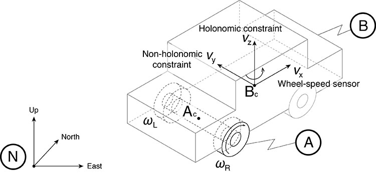
    INS/GNSS/WSS/VDC Integration. For the vehicle in motion, we developed a model consisting of a WSS measurement in the along-track direction, a non-holonomic constraint resisting lateral sliding, and a holonomic constraint on vertical movement (see FIGURE 4).

    The INS/GNSS/WSS/VDC integration using the EKF consists of the process model and the measurement models.

    FIGURE 4. The measurement model consisting of the WSS measurement in the along-track direction (vx), non-holonomic constraint resisting lateral sliding (vy), and holonomic constraint on vertical movement (vz). N is the navigation frame, Ac is the rear-axle center point and Bc is the center point of the body-fixed frame. (Image: Authors)
    FIGURE 4. The measurement model consisting of the WSS measurement in the along-track direction (vx), non-holonomic constraint resisting lateral sliding (vy), and holonomic constraint on vertical movement (vz). N is the navigation frame, Ac is the rear-axle center point and Bc is the center point of the body-fixed frame. (Image: Authors)

    INS/GNSS/SMC Integration. The static mode constraint provides zero-velocity measurements to the EKF measurement update to mitigate position error propagation. We use SMC only when it is known that the vehicle is not moving; for example, when the vehicle is in the parking gear.

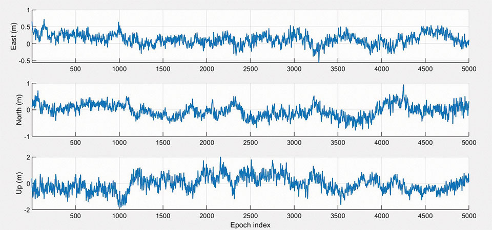
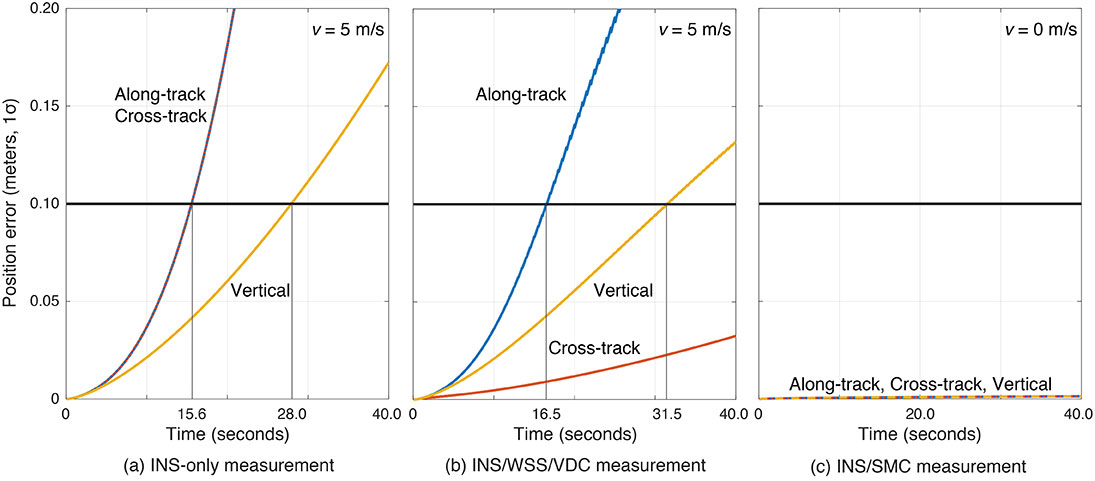
    Error Propagation Analysis. We tested the time from perfect initialization to when position error exceeds 0.1 meters in GNSS-denied environments. FIGURE 5 shows the error growth in the along-track (x), the cross-track (y) and the vertical (z). The error specifications for a STIM300 tactical-grade IMU are used in this analysis. The standard deviation of the WSS measurement noise is assumed to be 0.05 meters per second, and the standard deviation of the movement constraint violations is 0.001 meters per second. The vehicle is moving at 5 meters per second except when we test the SMC.

    The INS can coast 15.6 seconds before the position error standard deviation exceeds 0.1 meters in both the along-track and the cross-track directions (see FIGURE 5a). The INS/WSS/VDC can coast 16.5 seconds in the along-track direction, and significantly more than 40 seconds (the simulation duration) in the cross-track direction (see FIGURE 5b). In static mode, INS/SMC estimate errors do not grow with time in any direction, as expected (see FIGURE 5c). In GNSS-denied environments, the non-holonomic constraint suppresses the cross-track position error, but the WSS measurement hardly affects the along-track position error. The SMC works perfectly, but the usage is limited to when the vehicle is known to be stationary.

    FIGURE 5. The vehicle position error growth vs. time in the along-track (x), cross-track (y) and vertical (z) directions. Each graph represents the navigation system introduced in the multi-sensor integration section. The vehicle is moving at 5 meters per second (a and b) or 0 meters per second (c). (Image: Authors)
    FIGURE 5. The vehicle position error growth vs. time in the along-track (x), cross-track (y) and vertical (z) directions. Each graph represents the navigation system introduced in the multi-sensor integration section. The vehicle is moving at 5 meters per second (a and b) or 0 meters per second (c). (Image: Authors)

    SIMULATION SCENARIO

    We imagine a future driverless-car mission scenario in which multi-sensor navigation systems are practicable. To minimize congestion in a city, autonomous vehicles will be held outside the urban core when not in use. In the clear open-sky environment, a vehicle in a parking lot completes GNSS initialization using the INS/GNSS/SMC system. Once requested for action, the vehicle departs for the city from the parking lot, and the motion of the vehicle improves alignment by the INS/GNSS system. Safe navigation can be ensured using the system to provide continuity under overpasses and bridges in the open-sky environment. Upon entering the urban core, navigation becomes more dependent on the INS/WSS/VDC system.

    A reasonable numerical target for differential GNSS initialized position error is 0.02 meters, and for the INS alignment yaw angle error 0.1 degrees.

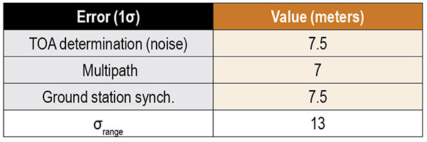
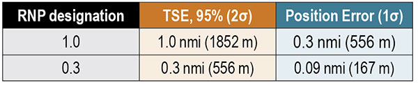
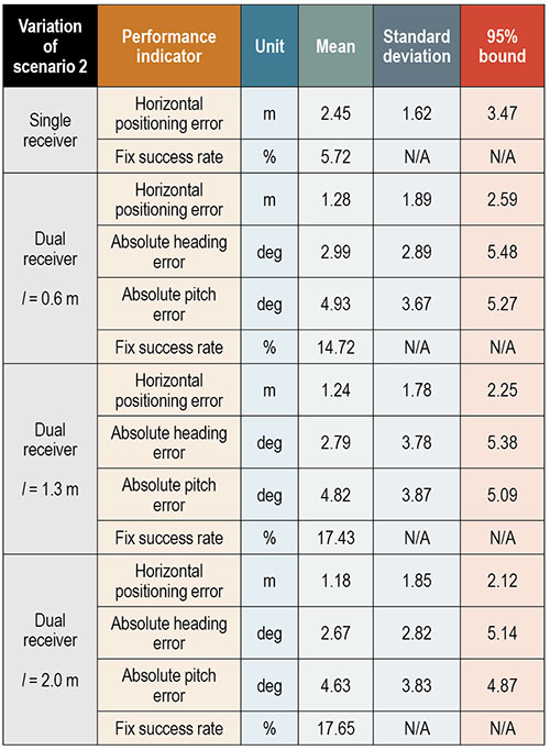
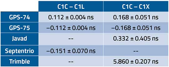
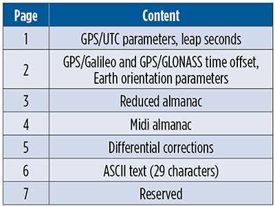
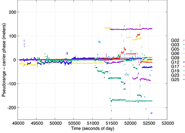
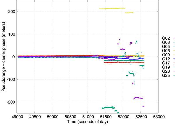
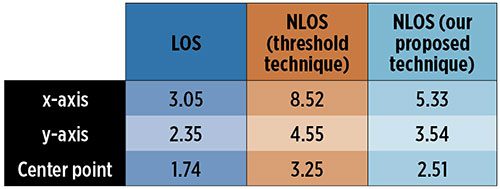
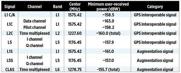
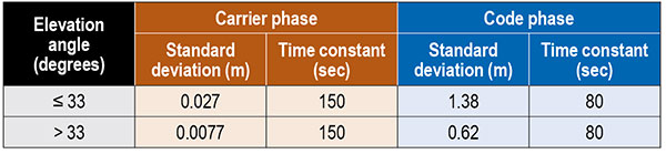
    Local GNSS multipath errors from nearby vehicles will vary with the satellite elevation angle. Prior experimental results show that lower elevation-angle satellite signals (below 33 degrees) are much more likely to be impacted by multipath than higher ones (see TABLE 1).

    Table 1. The nominal GNSS multipath error values in the simulation.
    Table 1. The nominal GNSS multipath error values in the simulation.

    INITIALIZATION AND ALIGNMENT

    Initialization takes place in a parking lot with a clear sky view. A vehicle is in the parking gear, enabling SMC to be applied. FIGURE 6a shows a typical example: with INS/GPS/SMC, system initialization takes about 31 minutes, and with INS/GPS, about 36 minutes. Therefore, SMC does speed up GPS initialization, although the improvement is modest.

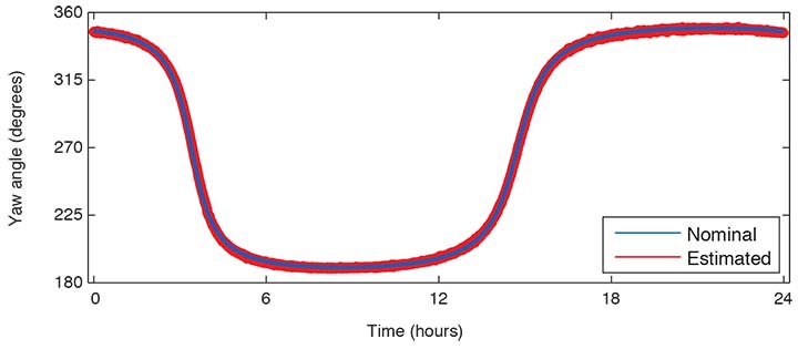
    The yaw angle is not aligned during the initialization, but roll and pitch are immediately aligned (see FIGURE 6b). Earth’s gravity affects roll and pitch angle alignment but not yaw angle.
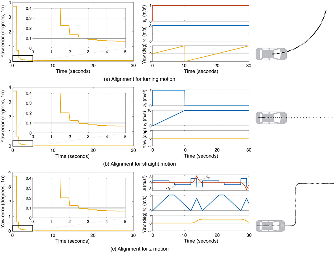
    Yaw angle alignment cannot be performed when the vehicle is stationary or moving with constant velocity. Accelerated motion, either straight or turning, is required.

    FIGURE 6. (a) Comparisons of initialization time between INS/GPS and INS/GPS/SMC in an open-sky environment. The INS/GPS/SMC system initializes rapidly. (b) Transitions of roll, pitch, yaw alignment during the initialization. Yaw angle alignment cannot be performed when the vehicle is stationary. (Image: Authors)
    FIGURE 6. (a) Comparisons of initialization time between INS/GPS and INS/GPS/SMC in an open-sky environment. The INS/GPS/SMC system initializes rapidly. (b) Transitions of roll, pitch, yaw alignment during the initialization. Yaw angle alignment cannot be performed when the vehicle is stationary. (Image: Authors)

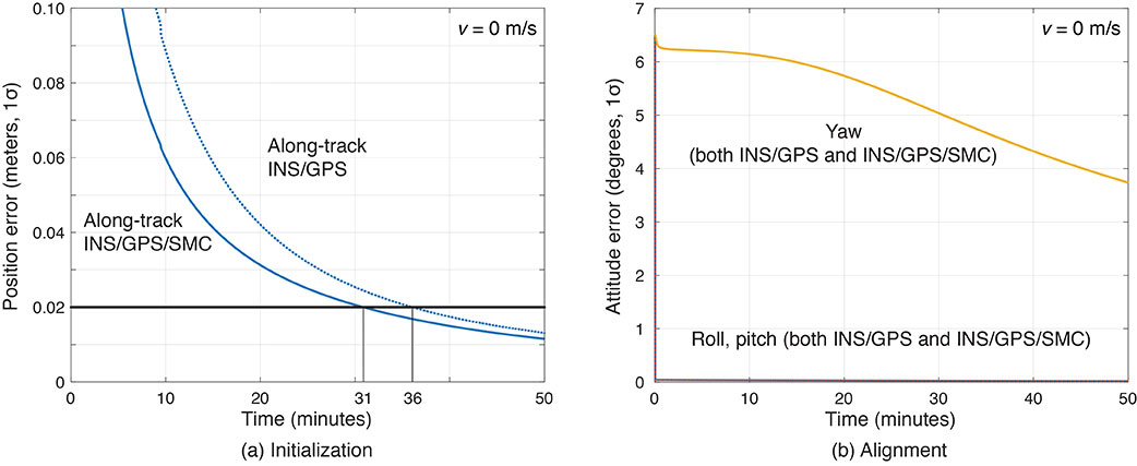
    FIGURE 7 shows the behavior of the yaw angle error standard deviation using the INS/GPS system when centripetal (see FIGURE 7a) or tangential (see FIGURE 7b) acceleration is applied. The yaw angle can be aligned in a couple of seconds for either type of acceleration. To represent typical initial motions of self-driving cars, we model a parking-lot departure via a “Z”-shaped path. In this scenario, the yaw alignment error reaches 0.1 degrees within a couple of seconds (see FIGURE 7c).

    FIGURE 7. The behavior of yaw angle error when centripetal (a) or tangential (b) acceleration is applied; (c) shows the behavior while following a z-shaped path. The yaw angle can be aligned in a couple of seconds in each case. (Image: Authors)
    FIGURE 7. The behavior of yaw angle error when centripetal (a) or tangential (b) acceleration is applied; (c) shows the behavior while following a z-shaped path. The yaw angle can be aligned in a couple of seconds in each case. (Image: Authors)

    EVALUATION IN URBAN ENVIRONMENTS

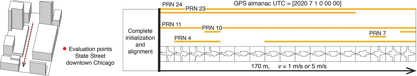
    After initialization and alignment in the open-sky environment, we simulated the vehicle traveling into the urban core. The urban environment in our study is 3D-mapped State Street in Chicago, which runs north-south and transits from low-rise neighborhoods to central downtown. We selected one congested section surrounded by tall buildings and computed the position error standard deviation along the path. The evaluation points are at 10-meter intervals over a total distance of 170 meters. The yellow lines in FIGURE 8 denote the visible satellites, identified by their pseudorandom noise (PRN) code numbers, at each point. We assume for convenience that the INS/GPS system is initialized and aligned at the first evaluation point. In reality, we would expect a degraded initial condition because we are starting the simulation in an urban canyon.

    FIGURE 8. Evaluation points and PRN numbers of visible satellites at each point. (Image: Authors)
    FIGURE 8. Evaluation points and PRN numbers of visible satellites at each point. (Image: Authors)

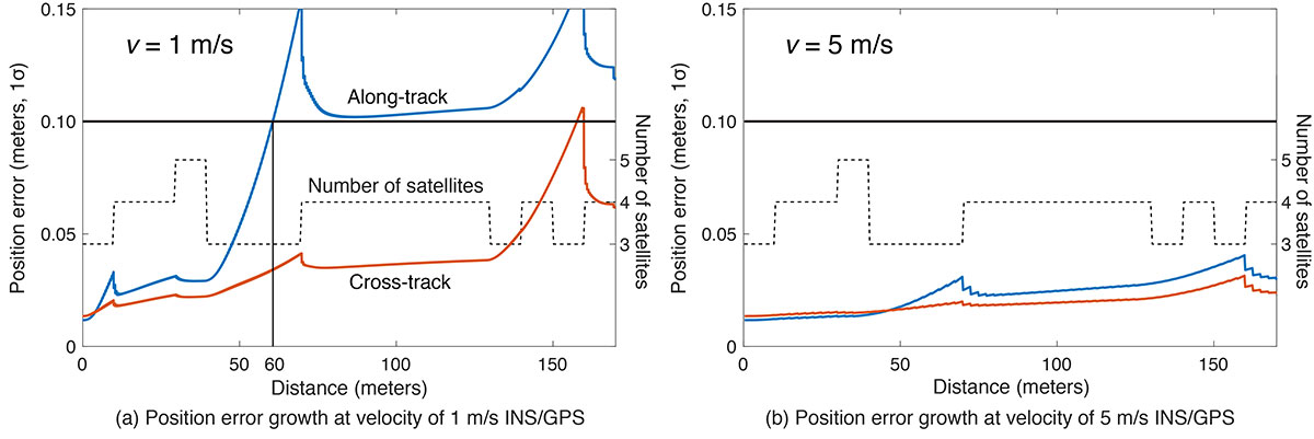
    In the first simulation, the car equipped with the INS/GPS system moved either 1 or 5 meters per second. The y-axis in FIGURE 9 represents the position error standard deviation, and the x-axis represents the distance in meters. The dotted line expresses the number of visible satellites. The error when the vehicle velocity is 1 meter per second exceeded the maximum allowable position error standard deviation of 0.1 meter, at the distance of 60 meters. However, when the velocity was 5 meters per second, the maximum allowable position error standard deviation was never reached. It is also clear from the figures that error propagation is significantly affected by the number of visible satellites.

    FIGURE 9. A comparison of position error growth between velocities of 1 meter per second and 5 meters per second. (Image: Authors)
    FIGURE 9. A comparison of position error growth between velocities of 1 meter per second and 5 meters per second. (Image: Authors)

    In the second simulation, we compared two different navigation systems, INS/GPS and INS/GPS/WSS/VDC. The vehicle moved at 1 meter per second in the same urban environment. The INS/GPS/WSS/VDC system does provide relief, but the error propagation is still clearly affected by the number of visible satellites (see FIGURE 10).

    FIGURE 10. A comparison of position error growth between the INS/GPS and INS/GPS/WSS/VDC systems for a velocity of 1 meter per second. (Image: Authors)
    FIGURE 10. A comparison of position error growth between the INS/GPS and INS/GPS/WSS/VDC systems for a velocity of 1 meter per second. (Image: Authors)

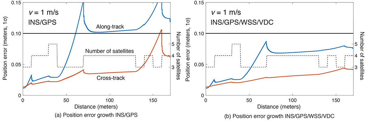
    In GNSS-challenged environments, INS error propagation is a function of time. When a vehicle moves faster, it clears the blockage area more quickly, reducing the impact of INS drift — a function of time, not distance. In contrast, GNSS error is completely determined by location. Because INS error propagation depends on how long the vehicle stays in an area of GNSS outage, protection levels for trips through the same area will be different if the vehicle is smoothly cruising or gets stuck in a traffic jam.

    CONCLUSION

    To gain a better understanding of how long and under what local conditions multi-sensor integrated navigation systems can maintain fault-free integrity, we evaluated navigation positioning errors in 3D-mapped downtown Chicago. The system we developed consists of sensors with which self-driving cars would reasonably be equipped: GNSS, INS, WSS and dynamic constraints. We showed that INS/GPS position errors along the path depend very strongly on the vehicle’s speed. When the system is augmented with WSS/VDC, position errors are suppressed, but the error propagation is still strongly influenced by the number of visible satellites.

    ACKNOWLEDGMENTS

    The research described in this article is supported by the National Science Foundation. Figure 1 was created by Alexis Arias of the Landscape Architecture + Urbanism Program at the Illinois Institute of Technology (IIT). The authors greatly appreciate the advice and help of Nilay Mistry from that program.
    This article is based on the paper “Evaluating INS/GNSS Availability for Self-Driving Cars in Urban Environments” presented at ION ITM 2021, the virtual 2021 International Technical Meeting of The Institute of Navigation, Jan. 25–28, 2021.


    KANA NAGAI is a Ph.D. candidate and research assistant in mechanical and aerospace engineering at IIT.

    MATTHEW SPENKO is a professor of mechanical and aerospace engineering at IIT. He earned his M.S. and Ph.D. degrees in mechanical engineering from the Massachusetts Institute of Technology.

    RON HENDERSON is a professor and director of the Landscape Architecture + Urbanism Program at IIT. He earned his Master of Landscape Architecture and Master of Architecture from the University of Pennsylvania.

    BORIS PERVAN is a professor of mechanical and aerospace engineering at IIT. He earned his M.S. from the California Institute of Technology and Ph.D. from Stanford University.

  • Innovation: Mode N provides alternative PNT for aviation

    Innovation: Mode N provides alternative PNT for aviation

    Photo: guvendemir/E+/Getty Images
    Photo: guvendemir/E+/Getty Images

    By Brandon Weaver, Gianluca Zampieri and Okuary Osechas

    Innovation Insights with Richard Langley
    Innovation Insights with Richard Langley

    IT’S A FACT. GPS and its brethren global (and regional) navigation satellite systems are susceptible to outages caused by both natural and engineered events. Several reports issued in the past couple of decades have documented the vulnerability of GNSS. Twenty years ago this past August, the U.S. Department of Transportation’s John A. Volpe National Transportation Systems Center issued a report, commonly referred to as the Volpe Report, in which they found that “GPS service is susceptible to unintentional disruptions from ionospheric effects, blockage from buildings, and interference from narrow and wideband sources.” Although not explicitly mentioned in the report, besides emissions from communications systems, wideband interference can come from solar radio noise storms overpowering GPS signals. The report also highlighted that the “GPS signal is subject to degradation and loss through attacks by hostile interests. Potential attacks cover the range from jamming and spoofing of GPS signals to disruption of GPS ground stations and satellites.”

    The Volpe Report recommended a number of actions to mitigate the vulnerabilities of the GPS signal to disruption or loss, including the need for backups for positioning, navigation and timing — particularly for GPS applications involving the potential for life-threatening situations such as the loss of GPS use for safety-of-life navigation, which would include, for example, aircraft navigation.

    With the introduction of GPS (and subsequently the other GNSS and their augmentations) and its widespread adoption by the aviation industry, legacy navigation systems such as Omega, aviation radiobeacons, VHF Omnidirectional Range (VOR) and Distance Measuring Equipment (DME), were either shut down, reduced in their number of installations, or displaced as the primary method of navigation. These systems could not offer the same capabilities as GNSS, and that has led to the high reliance now on GNSS for getting aircraft safely from one airport to another.

    But as the Volpe Report pointed out, GPS and (by inference) all other GNSS are susceptible to outages, and so a reliable alternative PNT system that can be readily used for aircraft navigation is needed. Deutsche Flugsicherung, the German air traffic control organization, has proposed such a system, called Mode N. It builds on some aspects of existing navigation systems and aviation-certified signals not originally intended for navigation, including some used for communications and surveillance.

    In this month’s column, a team of researchers from the German Aerospace Center introduce us to Mode N, looking at its signal format, required ground infrastructure, aircraft avionics and the potential position accuracy this system could offer.


    To accommodate the continued growth of air traffic, air navigation service providers (ANSPs) are planning and implementing programs to increase the capacity and efficiency of airspace. These programs, which include the Next Generation Air Transportation System (NextGen) led by the U.S. Federal Aviation Administration (FAA) and the Single European Sky ATM (Air Traffic Management) Research Programme (SESAR) commissioned by the European Union, heavily rely on GNSS to enable certain capabilities to reach program goals. While intended to serve as the primary source of positioning, navigation and timing (PNT) for aviation services going forward, GNSS is vulnerable to sources of interference. For this reason, efforts have been taken to identify and develop an alternative PNT (APNT) system that can maintain capabilities supported by GNSS when a GNSS outage occurs.

    The ANSP for Germany, Deutsche Flugsicherung (DFS), has proposed a concept for such a system that they call Mode N. The proposed design leverages current navigation and surveillance technology to provide a completely new solution to navigation. As the current APNT environment is filled with a variety of proposed solutions spanning the entire field of communications, navigation and surveillance (CNS) technologies, it is useful to describe Mode N within the context of these other APNT systems. This contextual description serves to highlight the interaction of Mode N with current aviation systems — an important consideration for any system intended to serve aviation users. Additionally, as the Mode N design uses similar technological principles as other navigation and surveillance systems, the extensive research performed for APNT can be applied to the Mode N design to provide a preliminary assessment of its navigation performance over Germany.

    Development of APNT

    The current state of aviation navigation can be simplified by acknowledging that GNSS has replaced legacy navigation systems such as Distance Measuring Equipment (DME) and VHF Omnidirectional Range (VOR) beacons as the primary method of navigation for aircraft. GNSS PNT services enable many capabilities in the airspace that are relied upon by modernization efforts to accommodate the expected increase in air traffic in a safe and efficient manner. Because of GNSS vulnerabilities outlined in the 2001 Volpe Report, it was recognized that an alternative system that could enable the same capabilities as GNSS would be necessary to continue safe and efficient operation of airspace as envisioned if GNSS is unavailable.

    Proposed APNT solutions are generally sourced from the existing CNS environment. A common strategy is to use an aviation-certified signal not originally intended for navigation, which we have termed repurposed aviation signals (RAS). Other proposals include improving legacy systems, transmitting the ground-computed position to an aircraft, and creating new systems entirely. These sources of APNT are summarized in FIGURE 1 with explanations of the abbreviations to follow.

    FIGURE 1. Sources of APNT for navigation. (Image: Weaver et al)
    FIGURE 1. Sources of APNT for navigation. (Image: Weaver et al)

    A natural candidate for APNT is the use of existing non-GNSS navigation infrastructure. Prior to GNSS, VOR beacons providing beacon-relative heading information and DME navaids supplying two-way range information were the primary navigation infrastructure. Improvement in DME avionics enabled tracking of multiple DME stations, providing a DME-only position solution referred to as DME/DME. Adding DME ground stations and upgrading existing hardware to increase accuracy and coverage of DME/DME positioning was therefore an attractive APNT option.

    Another option sourced from the existing navigation infrastructure was to use RAS for positioning. One such RAS is that of the DME reply signal to a non-existent aircraft. By triggering DME responses in a desired fashion, aircraft can use the triggered responses for passive ranging without any change to the DME ground stations.

    Communication systems for aviation are also undergoing modernization efforts. Future communication systems (FCS) are being developed to provide broadband communication capability between aircraft and controllers.

    Surveillance is the domain of ground-based systems that determine the position of remote objects and is fundamental to allowing safe spacing of aircraft. Its origins reside in the development of primary radar, which was then complemented with secondary surveillance radar (SSR). Both primary radar and SSR use a rotating antenna to measure range and bearing to determine the location of the remote objects. Radar systems tend to be clustered around airports, limiting their area of coverage. To expand coverage in challenging terrain where radar is difficult to install, a technique known as multilateration is used, where a surveillance ground system can receive a signal from an aircraft and determine its position by comparing the time of arrival (TOA) of the signal between its ground stations. These systems were considered as a source of APNT by providing the aircraft position computed on the ground back to the aircraft via data uplink, but timely authentication and integrity concerns have stalled this approach in the United States.

    Surveillance RAS for APNT. The other branch of surveillance-sourced APNT is by using RAS, and this is very relevant to the design of Mode N. The system providing many of the RAS for navigation is ADS-B. With this service, an aircraft broadcasts its GNSS-derived position (ADS-B Out) to ground-based stations and any aircraft capable of receiving ADS-B transmissions. ADS-B is an important part of airspace modernization strategies; it is mandated for aircraft operating in most U.S. airspace, with European mandates following suit. ADS-B ground stations, referred to as ground-based transceivers (GBT) or radio stations (ADS-B RS), collect ADS-B Out messages for use by air traffic operators. These ADS-B RS also provide their own transmissions for use by aircraft that can receive ADS-B broadcasts (ADS-B In capability) and include weather information, nearby air traffic and so on.

    ADS-B can use different protocols to transmit its signals. The Mode S (S for selective) protocol was designed to allow SSR ground stations to selectively interrogate aircraft in their coverage area, reducing congestion on the reply frequency. The Mode S reply format consists of a four-pulse preamble and a data block containing either 56 or 112 information bits for the aircraft to provide information dependent on the interrogation received. Mode S is internationally standardized, and an extended format known as Mode S Extended Squitter was adopted for Automatic Dependent Surveillance Broadcast (ADS-B) services. Mode S Extended Squitter or 1090ES (as it’s transmitted exclusively on 1090 MHz) is also used by the ADS-B RS that rebroadcast ADS-B Out (ADS-R) and provide traffic information services (TIS-B) to nearby aircraft with ADS-B In capability.

    Another protocol, used in the United States, is the Universal Access Transceiver (UAT) format. Like 1090ES, UAT is used by certain aircraft to transmit their ADS-B Out messages. Similarly, ADS-B RS transmits TIS-B and ADS-R messages with the UAT protocol; it also includes additional information that it transmits with the Flight Information Service – Broadcast (FIS-B). UAT signals are transmitted in the United States on an unused DME channel frequency of 978 MHz. FIGURE 2 summarizes the relationship between these surveillance signals and the services that use them.

    FIGURE 2. Services using Mode S and UAT signal formats.(Image: Weaver et al)
    FIGURE 2. Services using Mode S and UAT signal formats.(Image: Weaver et al)

    Research investigating the ground-transmitted (ADS-B RS) 1090ES and UAT signals for ranging measurements greatly supports the assessment of Mode N presented here, as the Mode N system operates on a similar basis with a signal that blends characteristics of 1090ES and UAT.

    Mode N Overview

    Mode N (N for navigation) is a passive ranging system concept from DFS that seeks to provide APNT while reducing the spectrum congestion caused by existing aeronautical navigation and surveillance systems. The design includes the possibility for two-way and air-to-air ranging, but this overview focuses on the preferred passive mode of operation. It is designed around the Mode S format, which as mentioned, is used for SSR and ADS-B services. Despite early references to an SSR/N system, Mode N is not a new SSR mode but rather a new navigation system.

    The basic concept is for Mode N ground stations to transmit on a single frequency signals that include ground station ID/coordinates, allowing aircraft with Mode N avionics to receive those signals and determine position in a similar manner to GNSS. As a single frequency is desired to minimize spectrum usage, the ground stations would space their transmissions apart to avoid intersystem interference. This scheme, known as time division multiple access (TDMA), would require information within the signal message on the scheduled time a ground station transmits, which the Mode N format allows.

    Because Mode N shares many design aspects with Mode S, DME and other surveillance RAS, it is able to leverage previous APNT work for the benefit of its own analysis. Therefore, the overview of the design is described here relative to other APNT systems, as this is the basis of the preliminary performance assessment we present.

    The Mode N Signal. The Mode N design proposes using the Mode S downlink signal format as the basis for its ranging signal to be used by the aircraft for passive position determination, with some key differences. The frequency channel on 1090 MHz is too congested to accommodate more signals; thus, the first difference is that Mode N intends to transmit on a different frequency. While the channel selection is still ongoing, unused DME channels have been identified as options for frequency allocation.

    The second difference is the message content. As the Mode S downlink format transmits mainly aircraft-specific information, Mode N ground transmitters would instead populate their messages with information needed for passive ranging: ground station coordinates and time of transmission (TOT). The study of 1090ES messages (which also contain aircraft-specific information despite being transmitted by ground stations) as RAS required some special techniques to first identify which station was transmitting the message. The TOT is not present in 1090ES signals, but more importantly the time of transmission is not synchronized to any consistent reference. Aside from transmission frequency and message content, the Mode N signal design follows the Mode S downlink format (modulation, pulse shape and so on).

    The Mode N signal also shares some aspects with the UAT signal, particularly the FIS-B segment. First, UAT is also transmitted in the United States on an unused DME channel. The FIS-B message, which provides weather information, transmits the ground station coordinates and information that can be used to estimate the TOT. Specifically, UAT messages are synced to UTC, and each ADS-B RS has a designated time slot within a one-second interval where it transmits its FIS-B message. This time slot is included in the message, and can be used to determine the TOT of the signal. Mode N is designed to work in this exact manner, minus the weather information. One crucial difference between UAT and the Mode N design is the type of modulation. Like Mode S, Mode N proposes using pulse-position-modulation (PPM) or on-off keying (OOK). The resulting wider bandwidth — estimated to be less than 4.6 MHz at –3dB — has better resistance to multipath, whereas UAT is frequency modulated to maintain a narrow bandwidth to avoid interference with DME and is more susceptible to multipath. Research on UAT signals for pseudoranging capability (also determined at a higher update rate than once per second) would be necessary for navigation, an important consideration for the final Mode N design.

    Ground Infrastructure. The Mode N design, while based on RAS from the surveillance capability, requires new ground stations to transmit the Mode N signal. Requirements for the ground stations are that they provide adequate coverage to meet the requirements of an APNT system and that they are sufficiently synchronized in time. An initial time-synchronization scheme is the use of a radio frequency (RF) network consisting of the ground stations themselves, which requires radio line-of-sight of stations throughout the network. DFS performed a study and found that additional time-beacon stations would be necessary to maintain this RF time network, even though navigation coverage was provided using existing DME sites as hypothetical Mode N stations. Since these aspects of the design are still developing, the preliminary assessment we present assumes a network layout and time synchronization tolerance. As the Mode N design blends various CNS principles, a natural baseline design for the ground station locations consists of existing DME and surveillance sites in Germany. Using these locations for the ground stations enables computation of a horizontal dilution of precision (HDOP) at discrete locations throughout Germany. The assumed time synchronization is discussed further when developing a model of the Mode N ranging accuracy.

    Avionics. An interesting aspect of the Mode N design is its proposed avionics unit. The Mode N avionics must be capable of receiving Mode N messages, which it can do with the existing DME antennas on aircraft. The Mode N avionics unit must then decode the messages for position determination. Its active mode for two-way and air-to-air ranging would require the Mode N avionics to transmit Mode N messages, again using the existing DME antenna.

    Recognizing the continuing investment in the DME network by multiple countries, the Mode N avionics sensor is essentially built around a fully functional DME unit. This is intended to provide a seamless transition as Mode N stations are brought on line. The design of the avionics has little effect on the coverage assessment, aside from guaranteeing a minimum level of performance based on the current DME network, but is an important part of the implementation strategy. Furthermore, this blend of avionics has also been proposed for a unit compatible with DME and ADS-B (1090ES and UAT) signals.

    Preliminary Coverage Assessment

    Preliminary coverage assessments are a typical method to determine the feasibility of a proposed system to provide the required level of performance over a given area. A simple method of characterizing the position performance is in terms of the linear relationship between range error and DOP, where the range errors are assumed to be zero-mean, uncorrelated, and have identical distributions.

    As the aircraft is assumed to have additional sensors for determining its altitude, HDOP is commonly used to characterize the expected horizontal position performance.

    With range measurements, HDOP is a function of the transmitter geometry available to an aircraft at a given point. It is a straightforward computation to perform for a grid of points over the area of interest. The HDOP computation does depend on the type of range measurement, so passive (pseudo-) range, two-way range, and time difference of arrival (TDOA) measurements all have their corresponding DOP computation. Determining a model for the range error is less straightforward, and assessing the coverage potential of Mode N requires an estimation of the expected range error.

    Modeling Mode N Range Accuracy. As Mode N is not an existing system, abundant quantities of real measurements are unavailable for empirically characterizing the range performance. However, since Mode N is heavily based on the Mode S signal format and functions similarly to the DME and UAT signals, which all exist and have been measured extensively, research investigating those signals can help derive the model for the Mode N range performance.

    An alternate approach is to reference the standards for a specified performance level. For example, ICAO documentation specifies that the Airborne Collision Avoidance System (ACAS) logic use a zero-mean normal distribution range error model with a standard deviation of 50 feet, or about 15 meters. As ACAS also uses the Mode S signal format, this appears to be a reasonable source for the Mode N range error. However, since ACAS is an airborne two-way surveillance method, it does not exactly translate to a ground-based passive TDOA system such as Mode N. The 15-meter standard deviation is still useful, as it provides a check on the estimated Mode N accuracy. Other specifications suffer from similar drawbacks — Mode N does not directly apply to any single system. Thus, we apply the blended approach using previous APNT research.

    The fundamental measurement for the passive ranging mode of Mode N is the TDOA between pairs of ground stations. This measurement is in seconds, and is translated to a range difference by using the speed of radio signal propagation in a vacuum. (See our conference paper for further details.)

    Errors can be present in the TOA measurement, synchronization of the nominal TOT of the signals, and parsing of the time slot data field. The TOA measurement can have errors by inaccurate determination of the actual TOA due to noise or multipath and by the actual TOA differing from the nominal arrival time of the signal due to atmospheric delay. For terrestrial systems, propagation errors are considered to be dominated by multipath, so we don’t consider atmospheric effects here. Time synchronization errors are very important to the ranging accuracy, but it is assumed the time slot data field is parsed accurately. Other sources of error, such as inaccurate ground station coordinates, can affect the position error but have no effect on the range error. Additionally, the error originating from the change in aircraft position between reception of signals at ground stations is not considered in this article. The model of range accuracy can then be expressed as the root-sum-square (RSS) of the dominant individual error components.

    We studied each error component in isolation, selecting the applicable APNT research to leverage based on the Mode N design aspect that most corresponds with that error.

    Since the Mode N design also uses a pulsed signal, the evaluation of DME (specifically, DME/N) ranging performance is the starting point for estimating the TOA noise error. Part of the APNT effort was evaluating current DME performance, as it was thought it exceeded the specified performance in standards. A study found that current DME performance allowed a budgeted TOA error of 15 meters, 2σ.

    For the Mode N error model, a 7.5-meter error is an attractive option to choose as it is the average of two other sources and is the most recent. This value is a conservative estimate of the TOA accuracy for Mode N because the Mode N/S pulse shape is narrower than the DME pulse with a greater bandwidth, improving theoretical accuracy. For the preliminary coverage assessment, a conservative estimate is desired, because the actual TOA accuracy will vary over an area depending on transmitter distance — which impacts the level of signal noise. Note that the DME TOA errors are not divided by two as is done for the total DME error as they apply to a one-way TOA measurement.

    After assessing the relevant studies, we modeled the multipath component of the error following that from Mode S as 7 meters, 1σ.

    The final error component to estimate for Mode N is that of the synchronization of the ground stations. Based on the results from studies of the UAT signal and those from eLoran, we set a 15-meter maximum bias as a 2σ error component in the Mode N error model.

    Our error analysis is summarized in TABLE 1.

    Table 1. Predicted Mode N range accuracy. (Data: Weaver et al)
    TABLE 1. Predicted Mode N range accuracy. (Data: Weaver et al)

    A total 2σ error for current DME performance of 92 meters has been established, which translates to 46 meters of range accuracy after dividing by two (since the DME signal is a two-way range). A substantial part of this error derives from the avionics bias, which is minimized for a “potential” DME error budget due to an assumed improved avionics performance. This results in a DME range 2σ error of 34 meters. We chose this value to compare as the effect of avionics has less of an impact in a passive ranging system such as Mode N.

    Range performance for UAT signals was evaluated with measurements showing 20-meter (1σ) error when compared to GNSS truth, not including large biases attributed to ground station synchronization or processing errors. The 1090ES signals do not have an inherent ranging capability, so the TDOA measurement error of two ground station signals to one receiving station is difficult to measure. Instead, researchers have measured the differential TOA (DTOA) of one ground station signal received by two (GPS-synchronized) receiving stations to first identify which station transmitted the signal. When compared to the true DTOA based on ground station and receiving station coordinates, the measurements contained small biases around 10 meters with a standard deviation also less than 10 meters. Being DTOA measurements, these do not contain ground station synchronization errors, so the reported standard deviations correspond mostly with propagation and determining TOA. The 10-meter DTOA 1σ error can still be converted to a range error resulting in 14 meters (2σ). These results are summarized in TABLE 2.

    Table 2. Comparison of Mode N with other APNT signals. (Data: Weaver et al)
    TABLE 2. Comparison of Mode N with other APNT signals. (Data: Weaver et al)

    Coverage Assessment. With the estimated ranging accuracy, a preliminary coverage over Germany could now be assessed. Using the current 29 surveillance site locations in Germany and assuming that a minimum of three stations is necessary for positioning, the estimated position accuracy is shown in FIGURE 3.

    FIGURE 3 Estimated position error (in meters) for aircraft within a 100 nautical mile coverage radius using existing surveillance sites as installation locations for Mode N ground stations. (Image: Weaver et al)
    FIGURE 3. Estimated position error (in meters) for aircraft within a 100 nautical mile coverage radius using existing surveillance sites as installation locations for Mode N ground stations. (Image: Weaver et al)

    The coverage assessment used a “flat” Germany model with the estimated range accuracy from the preceding section (13 meters, 1σ). Atmospheric and terrain considerations were not applied in the assessment. It is important to note that this level of coverage would degrade at lower altitudes.

    To determine whether this level of accuracy is sufficient for the airspace modernization efforts in Europe, the desired Required Navigation Performance (RNP) accuracy requirement must be examined. For RNP 1.0, where 1.0 refers to the required 95% or 2σ total system error (TSE) accuracy in nautical miles, the position error allocation is assumed to be 30% of the RNP/TSE value. The required position accuracy is shown in TABLE 3.

    Table 3. RNP required horizontal position accuracy. (Data: Weaver et al)
    TABLE 3. RNP required horizontal position accuracy. (Data: Weaver et al)

    From Figure 3, aircraft at altitudes within the service volume supported by a 100-nautical-mile coverage radius are capable of meeting the accuracy requirement for RNP 1.0 and 0.3 within most of Germany. Coverage along the border is unavailable as only German surveillance site locations were used.

    Conclusions

    Although our derivation of accuracy and the coverage assessment method we used made several simplifying assumptions, the results indicate that Mode N has the potential to be a feasible APNT system. To be a part of the modern airspace navigation infrastructure, additional accuracy requirements must also be met. The integrity requirement is harder to meet than accuracy, and requires either redundant information available to the aircraft for a receiver autonomous integrity monitoring-like algorithm or a ground-based monitoring/augmentation system. Perhaps the biggest challenge to implementing the Mode N infrastructure is maintaining an RF-based time synchronization network. Convincing aircraft operators to update their avionics is another challenge to Mode N implementation, although the inclusion of DME functionality in the Mode N avionics seeks to ease that transition.

    DISCLAIMER

    The views expressed herein are those of the authors and are not to be construed as official or reflecting the views of Deutsche Flugsicherung.

    ACKNOWLEDGMENT

    This article is based on the paper “An Overview of the Proposed Mode N System in the Context of Alternative Position, Navigation, and Timing (APNT) Development” presented at ION ITM 2021, the virtual 2021 International Technical Meeting of The Institute of Navigation, Jan. 25–28, 2021.


    BRANDON WEAVER is a researcher at the German Aerospace Center (DLR) and works on alternative navigation systems.

    GIANLUCA ZAMPIERI joined the Alternative Navigation Systems Group at DLR’s Institute for Communication and Navigation in 2019.

    OKUARY OSECHAS leads the Alternative Navigation Systems Group in the Institute of Communications and Navigation at DLR.


    Further Reading

    (to come)

  • Innovation: Attitude determination and RTK positioning using low-cost receivers

    Innovation: Attitude determination and RTK positioning using low-cost receivers

    Getting It Better

    Attitude Determination and RTK Positioning Using Multiple Low-Cost Receivers with Known Geometry

    By Xiao Hu, Paul Thevenon and Christophe Macabiau

    Innovation Insights with Richard Langley
    Innovation Insights with Richard Langley

    DO YOU HAVE THE BEST POSITION AND ATTITUDE? No, I’m not talking about your personal life. I’m talking about the location and orientation of a vehicle. We all know that GNSS, perhaps augmented with additional sensors, can provide the position of a vehicle accurate at the few-meter level or so under good conditions when using only single-frequency pseudorange measurements. After all, this is how most consumer-grade receivers work, including those embedded in cell phones. Yes, we can sometimes do better by using dual-frequency measurements such as those obtained by newer cellphone models with dual-frequency receivers, but we need to use carrier-phase measurements to get a significant improvement in positioning accuracy.

    But this is not news. That carrier-phase measurements had the capability to provide up to centimeter-level accuracy was demonstrated in the early 1980s, when only a few prototype GPS satellites were in orbit. Surveyors and geodesists developed a relative or differential positioning technique using a reference station and one or more rover stations to determine the three-dimensional baselines connecting the stations. Knowing the coordinates of the base station, the coordinates of a rover station could be determined. This use of differential carrier-phase measurements was actually pioneered in the radio astronomy community through the development of interferometric techniques for improving the resolution of radio telescopes, which led to the invention of very long baseline (radio) interferometry (VLBI) in 1967. Geodesists realized that the astronomers’ technique could be used to obtain very precise (and accurate) baselines between radio telescopes, even if they were on different continents.

    The surveyors and geodesists performing the initial baseline determinations using GPS carrier-phase observations even developed ingenious techniques for resolving the integer ambiguities that bedevil carrier-phase measurements. Those techniques evolved into the real-time kinematic or RTK positioning capability widely used today, as well as attitude determination. It was in March 2001 that we featured an Innovation article on GPS attitude determination. As we said, “[GPS] is well known for its ability to determine a platform’s position and velocity with high accuracy. Less well known is the ability of GPS also to provide the orientation of the platform. Using three or more antennas feeding separate receivers, or separate channels in a single receiver, the baseline vectors connecting the antennas can be determined. The directions of these vectors determine the platform’s three-dimensional orientation… If only two antennas are used, then only two angles or directions of the platform can be determined, such as the azimuth or heading of the platform and its elevation angle or pitch.”

    While RTK positioning and attitude determination is readily done with high-end equipment, it is still a challenge to get good results for kinematic platforms with low-cost receivers. In this month’s column, we learn how a team of researchers in France is trying to do just that.


    Over the past decade, GNSS has been commonly used in various domains: automotive, aviation, marine, precision agriculture, geodesy and surveying, and so on. This includes autonomous driving, which has become more and more a central topic for the automobile industry, a kind of application for which information about precise position and attitude is essential. However, the accuracy and integrity that a low-cost GNSS receiver can provide in a restricted urban or indoor environment is far from satisfactory for applications where bounded decimeter or centimeter accuracy is envisioned.

    To reach this level of accuracy, techniques using raw carrier-phase measurements have been developed. Such measurements are more precise than pseudorange (code) measurements by a factor of about a hundred. Nevertheless, they are also less robust than code measurements and include a so-called integer ambiguity that requires implementation of an integer ambiguity resolution (IAR) process to use them for positioning. In some harsh environments, severe multipath and losses of lock of the receiver tracking loops create carrier cycle slips, which result in sudden changes of these ambiguities. If not detected, cycle slips create a bias in the carrier-phase measurement resulting in a reduction of position accuracy. Even if a cycle slip is detected, the IAR process has to be, at least partially, re-initialized, leading also to a loss of positioning accuracy. To increase confidence and to accelerate the IAR process by limiting the search space, restrictions can be established by using an array of two or more receivers with prior known and fixed geometry, which includes the lengths of the baseline vectors between the antennas of the receiver array and the orientation of these vectors.

    In recent years, several studies have focused on the use of an array of receivers for attitude determination. However, to the authors’ knowledge, very few research articles can be found that address the use of an array of receivers to improve the accuracy of positioning or for some steps of precise position computation for real-time kinematic (RTK) processing with vehicle attitude determination, such as cycle-slip detection or integer ambiguity resolution. The objective of the research reported in this article is to explore the possibility of achieving precise positioning with a low-cost architecture: using multiple low-cost receivers with known geometry to enable vehicle attitude determination and improved RTK performance.

    SYSTEM GEOMETRY AND CONFIGURATION

    With the intention of performing precise attitude estimation, we have adopted a dual antenna set-up, where two GNSS antennas with a known baseline length are mounted on a vehicle’s rooftop to get an attitude estimation. Furthermore, the absolute position accuracy is augmented using the RTK approach, in which the vehicle is positioned relative to a third receiver, whose position is static and known, used as a virtual reference station (VRS). By knowing the position of the VRS, the vehicle can be positioned absolutely, too. In the positioning algorithm, we strongly rely on carrier-phase positioning which, thanks to its low noise characteristics, may enable decimeter-level positioning. FIGURE 1 shows the typical geometry of our measurement set-up.

    FIGURE 1. Geometry of the model including the definition of the attitude of the vehicle.
    FIGURE 1. Geometry of the model including the definition of the attitude of the vehicle.

    According to Figure 1, the two GNSS antennas on the vehicle’s rooftop span the array antenna baseline b12, which one can resolve for the Euler attitude angles to get the vehicle’s orientation (heading and pitch ).
    For each time epoch, we estimate both the RTK position and receiver array attitude. The baseline b13 spanned between one vehicle antenna and the VRS antenna enables us to locate the position of the vehicle relative to the VRS.

    MATHEMATICAL MODELS

    The realization of GNSS navigation is typically based on a Kalman filter, which is the most popular choice given its optimality and simplicity of implementation. In our study, we developed a position and attitude determination algorithm based on an extended Kalman filter (EKF).

    State Transition Model. The state transition or state-space model describes how the states or parameters of the system vary over time based on a specific linear model. In our EKF modeling, the state vector includes five vehicle state parameters and 2 × (Nsat – 1) satellite state parameters: the 3D position of GNSS receiver 1 relative to GNSS receiver 3 (), the pitch angle of the vehicle (), the heading angle of the vehicle (), the DD integer ambiguities of the visible satellites seen by GNSS receiver pair 1-3, and the DD integer ambiguities of the visible satellites seen by receiver pair 2-3. Note that at a given epoch, we can consider different sets of satellites visible for the receiver pairs.

    Transition Model for Position- and Attitude-Related State Parameters. In our EKF modeling for the position- and attitude-related state parameters, we suppose that they follow a random walk model, meaning that the speed and the angular rate are a zero-mean Gaussian process.

    Transition Model for Satellite-Related State Parameters. The satellite-related parameters are all assumed to be constant over subsequent epochs with very small noise compared to the position- and attitude-related state parameters. The resulting state transition matrix is then given by an identity matrix and different values of process noise variance are added to complete the model.

    Measurement Model. The measurement model describes how the individual sensor measurements are related to system states. In general, for every epoch, the measurement vector, which contains all measured values, can be described as a function of the state vector combined with the measurement noise vector, which describes the expected Gaussian noise of every measured value with an associated measurement noise covariance matrix.

    In our model, the measurement vector comprises the following measured values: the double-difference (DD) pseudorange (code phase) measurement vector of receivers 1 and 3, the DD pseudorange measurement vector of receivers 2 and 3, the DD carrier-phase measurement vector of receivers 1 and 3, and the DD carrier-phase measurement vector of receivers 2 and 3. The DD measurements are obtained by differencing the single-difference (SD) measurements in the usual way.

    In this measurement model, the position of receiver 2 is expressed in terms of the position of receiver 1 and the baseline vector between the two receivers of the array, such that it contains the known array baseline length information and the attitude information that we want to estimate. The individual DD corrected pseudorange and carrier-phase measurements for our short baseline case (less than 3 kilometers) can be modeled using certain approximations such as ignoring the tiny differential atmospheric effects.

    To reflect the difference in precision between the pseudorange and carrier-phase measurements, a fixed weighting factor of 1/100 is applied to the pseudorange.

    An elevation-angle-dependent measurement noise variance between all satellites is defined to complete the measurement model, defining the measurement covariance matrix.

    The relationship between the state and measurement vector is obviously non-linear, thus we need to linearize this measurement function and obtain the measurement (Jacobian) matrix for use in the EKF, as usual. Our algorithm is described in more detail in the proceedings paper on which this article is based (see Further Reading).

    Two alternating steps, which are the state prediction step and the state update step, are then conducted to complete the proposed EKF algorithm.

    RTK PROCESSING

    We first carry out a cycle-slip detection and repair scheme based on multi-epoch measurements. In our work, we use the differential phases over time cycle-slip resolution method. It is based on the observation of the differential phases between two adjacent epochs, which should include the actual jump in the ambiguity if there is one, plus some clock errors and the remaining noise term.

    Except for the ambiguity term, all terms contributing to the time-differenced phases change slowly. Any cycle slips will lead to a sudden jump in the time difference of the phases. Based on the past observation of differential phase measurements, a prediction of the current differenced data can be obtained by polynomial extrapolation or interpolation. The residual between the prediction and the observation can then be used as a detector metric, to be compared to the detection threshold to decide whether there are any cycle slips.

    After the cycle-slip detection process, a cycle-slip validation and size determination process is conducted to verify the determined sizes of the cycle slips. Cycle slips can be repaired using integer vector estimation similar to ambiguity resolution in the position domain.

    After repairing the existing cycle slips, the RTK processing begins. From the previously described EKF process, we first obtain a float estimation of the DD integer ambiguity. The accuracy of the position state estimate is further improved by fixing the DD ambiguities to integer numbers by using the well-known LAMBDA algorithm.

    The integer candidates are selected based on the sum of squared errors to get a fixed solution. The candidate with the lowest error norm is chosen once the ratio of the maximum a posteriori error norm between the second-best candidate and the best candidate is bigger than a threshold. It is a pre-defined critical value that the squared norm of ambiguity residuals of the best and second-best candidates should exceed to validate the integer estimation. In our work, we take an empirical fixed value of 3.0.

    Once the IAR process is declared successful, a new position is computed using the DD carrier phase measurements corrected by the validated DD integer ambiguities. This final position is a fixed solution. If the IAR process is not declared successful, the final position is kept as the float solution.

    SET-UP AND SCENARIOS

    In this section, we discuss the verification of our precise position and attitude determination algorithm with real measurements from two low-cost GNSS receivers and one high-end GNSS receiver.

    Data Collection. To investigate the feasibility of our proposed precise positioning and attitude determination algorithm, we set up a measurement campaign using four low-cost GNSS patch antennas and took measurements by recording single-frequency (L1) GPS pseudorange and carrier-phase measurements simultaneously at a 1-Hz rate. We put the patch antennas at various distances from each other, ranging from 60 centimeters to about 2.0 meters. In addition, we made the measurements in several different environments including an urban environment, a suburban environment, and an open-sky environment.

    FIGURE 2 shows a typical set-up of the GNSS antennas for one of the measurement sessions. According to Figure 1, any two GNSS antennas on the vehicle’s rooftop span the vehicle antenna baseline, which we can resolve for the pitch and heading attitude angles to get the vehicle’s orientation. Additionally, the baseline spanned between one vehicle antenna, and the VRS antenna is able to position the vehicle relative to the latter. If the VRS antenna location is known, the absolute position of the vehicle can be determined.

    FIGURE 2. Real data collection set-up: Four GNSS U-blox antennas and one NovAtel SPAN receiver antenna on the vehicle rooftop.
    FIGURE 2. Real data collection set-up: Four GNSS U-blox antennas and one NovAtel SPAN receiver antenna on the vehicle rooftop.

    The measurement test was performed with a vehicle on which the following hardware was mounted:

    • 4 low-cost GPS receivers with 1 Hz data rate
    • 4 L1 patch antennas mounted on the roof of the vehicle along its longitudinal axis
    • 1 high-end receiver on the roof of a building as the reference station for RTK processing
    • 1 high-end receiver tightly coupled with a tactical-grade inertial measurement unit with an antenna on the vehicle to provide its reference position and attitude.

    Data Collection Scenarios. We collected three sets of data in different environments for the analyses described in this article.

    Open-Sky Environment. To get an open sky and stable environment, the first measurement session took place on the football field of the École Nationale de l’Aviation Civile (ENAC) in Toulouse. As shown in FIGURE 3, the two receivers are static and their positions are fixed on the football field with favorable satellite visibility. This scenario was mainly used for validation of the algorithm implementation and to provide a reference for our multi-receiver system performance.

    FIGURE 3. Receiver fixed position for dataset 1.
    FIGURE 3. Receiver fixed position for dataset 1.

    Suburban Environment. The second measurement session took place on the ENAC campus. The true trajectory provided by the high-end equipment and the corresponding satellite visibility during the data collection are shown in FIGURE 4.

    FIGURE 4. Trajectory and corresponding satellite visibility for dataset 2.
    FIGURE 4. Trajectory and corresponding satellite visibility for dataset 2.

    Urban Environment. The third measurement session was performed when the vehicle was driven from ENAC to Toulouse’s city center. The whole trajectory in Google Earth and the corresponding satellite visibility during the data collection are shown in FIGURE 5.

    FIGURE 5. Trajectory and corresponding satellite visibility for dataset 3.
    FIGURE 5. Trajectory and corresponding satellite visibility for dataset 3.

    EXPERIMENTAL RESULTS AND DISCUSSION

    The datasets we collected allow us to investigate certain aspects of the simulations of our previous work. With our data collection approach, we could vary the distance between the two rover antennas, referred to as the array baseline length elsewhere in this article, as well as the type of environment. In this section, we address the following three points regarding the impact of these two aspects (array baseline and type of environment):

    • correlation of measurement error in the measurements collected by an array of receivers
    • improvement of cycle-slip detection and repair
    • improvement of positioning and attitude accuracy and ambiguity-fixed solution availability.

    Experimental Results on the Correlation of Measurement Errors. As the measurements come from signals received by the closely placed antennas, it is safe to consider a certain level of correlation between these measurements. For example, the multipath error from the same satellite may be similar in the measurements recorded by the receivers connected to the two closely-mounted antennas.

    By removing the corresponding geometric distance term from the DD pseudorange and carrier-phase observations, the correlation coefficient for the DD pseudorange and carrier-phase observations measured by the different antennas on the same satellite pair can be computed.

    We found that the DD phase measurement errors are very correlated, and there is also a medium degree of correlation between the pseudorange measurements. We speculate that this might be due to the characteristic of the GNSS DD measurements.

    To make our model closer to the real situation and thereby improve the EKF performance, we updated the observation covariance matrix in the EKF model by replacing the diagonal matrix with one including non-diagonal terms based on the correlation coefficient values we found.

    Experimental Results on the Cycle-Slip Detection Performance. We carried out a number of tests on our single-frequency method, which has many limitations. Due to the imperfect detection of cycle slips, a larger ambiguity standard deviation value of 0.1 cycle was chosen to account for possible undetected cycle slips. A slight improvement in positioning results was achieved compared with a smaller value of 0.01.

    Typical Positioning and Attitude Determination Performance. We found that the dual-receiver system performs better than the single-receiver situation and provides better solution availability thanks to the doubled observations redundancy.

    FIGURE 6 illustrates the 3D RTK positioning estimation error for our multi-receiver method. As one can notice, the algorithm succeeded in outputting a positioning result with an accuracy of about 0.5 meters for the horizontal coordinates, which is acceptable for a harsh environment.

    FIGURE 6. 3D RTK positioning estimation error illustration.
    FIGURE 6. 3D RTK positioning estimation error illustration.

    FIGURE 7 shows the estimation of the pitch and heading angles of the vehicle for dataset 1. One can see from the figure that the error between the estimated result and the true value is extremely small (less than 2 degrees), which can provide us with a relatively accurate vehicle posture by using our proposed method.

    FIGURE 7. Illustration of vehicle attitude estimation for dataset 1.
    FIGURE 7. Illustration of vehicle attitude estimation for dataset 1.

    Experimental Results of the RTK Performance. We found that for our open-sky data, the dual-receiver array system provides better performance than the single-receiver RTK solution, thus demonstrating the usefulness of such an approach.

    The results from the analysis of the datasets from the suburban and urban test drives gave us some useful information on the robustness of the multi-receiver RTK system in harsh environments.

    As previously mentioned, the suburban data was collected when the vehicle was driven on the ENAC campus. The reference trajectory was provided with centimeter-level accuracy. The maximum standard deviation values, up to 10 centimeters, occur at around the 500-epoch mark, which corresponds to the zone having a minimum number of visible satellites. Generally, however, the environment is quite favorable with at least eight satellites in view for most of the time.

    We have compared the results from the single-receiver system and our multi-receiver system in terms of the ambiguity fix success rate, the horizontal positioning (east and north directions), error statistics (mean, standard deviation, and 95% error bound), and array attitude error statistics for all three data collections. As an example, TABLE 1 gives the performance comparison between our dual-receiver system and the single-receiver system in the suburban environment and for different array baseline lengths. A better accuracy result is obtained in the dual-receiver situation.

    Table 1. Performance comparison for different array baselines for data collection 2 – Suburban.
    Table 1. Performance comparison for different array baselines for data collection 2 – Suburban.

    Moreover, there is no huge difference in the accuracy of the positioning results between the different dual-receiver variations. However, as expected, the attitude accuracy does improve slightly as the array baseline length increases.

    The high-end GNSS receiver with IMU provided a decimeter-level trajectory accuracy in the urban scenario. The number of visible satellites was much lower than for the other two environments. A clear uncertainty increase in the position solution was observed in the reference result during the trajectory section where the number of satellites was fewer than six. We also obtained satisfactory results from our urban scenario test. We can conclude that the use of an array of receivers with known geometry to improve RTK performance is feasible and effective.

    CONCLUSION

    In this article, we have presented a method that includes an array of receivers with known geometry to enable vehicle attitude determination and enhanced RTK performance in different environments. Taking advantage of the attitude information and the known geometry of the array of receivers, we are able to improve some of the steps of precise position computation.

    We demonstrated through real data processing results that our multi-receiver RTK system is more robust to degraded satellite geometry, in terms of ambiguity fixing rate, and obtains a better position accuracy under the same conditions when compared with the single-receiver system.

    ACKNOWLEDGMENTS

    The research described in this article was supported by the China Scholarship Council. The article is based on the paper “Attitude Determination and RTK Performances Amelioration Using Multiple Low-Cost Receivers with Known Geometry” presented at the virtual 2021 International Technical Meeting of The Institute of Navigation, Jan. 25–28, 2021.

    MANUFACTURERS

    Our equipment included four U-blox (www.ublox.com) F9P GNSS receivers fed by U-blox ANN-MB series multi-band patch antennas, a Hexagon | NovAtel (www.novatel.com) ProPak6 SPAN GNSS receiver with integrated tactical-grade IMU and a NovAtel Pinwheel GPS-702-GG antenna, and a Septentrio (www.septentrio.com) AsteRx-U GNSS receiver with a Hexagon | Leica (leica-geosystems.com) AR20 choke ring antenna as the base station for RTK processing.


    XIAO HU is a Ph.D. student in the Signal Processing and Navigation (SIGNAV) research group of the TELECOM laboratory at École Nationale de l’Aviation Civile (ENAC) in Toulouse, France.

    PAUL THEVENON is an assistant professor at ENAC.

    CHRISTOPHE MACABIAU is the head of ENAC’s TELECOM team, which includes research groups in signal processing and navigation, electromagnetics, and data communication networks.


    FURTHER READING

    (Coming soon)

  • In the beginning, there was innovation

    In the beginning, there was innovation

    1990: UNB Professor Richard Langley and two graduate students use a GPS antenna (recognize it?) on a tripod to re-measure a historical baseline. (Photo: UNB Perspectives)
    1990: UNB Professor Richard Langley and two graduate students use a GPS antenna (recognize it?) on a tripod to re-measure a historical baseline. (Photo: UNB Perspectives)

    When GPS World published its first issue in January 1990, only 15 GPS satellites had been launched, including the 10 prototype or Block I satellites. And four of those early satellites had ceased operation. But there had been enough satellites in orbit for more than a decade to permit early commercial and scientific use of the system. There were even handheld receivers for personal navigation, albeit somewhat larger than those we have today. But it was clear that GPS was going to take off in a big way, and that there was a business case for launching a monthly magazine (bimonthly in its first year) about GPS for professionals in the positioning, navigation and timing communities.

    The new magazine was to feature a blend of news, product announcements and articles about GPS, including cutting-edge research on GPS technology and its applications taking place at universities and research institutes around the world. That is why Glen Gibbons, the founding editor of GPS World, reached out to the University of New Brunswick (UNB), an early leader in GPS research and education, to manage a column to be called simply “Innovation.” Glen stipulated that “the column should deal with issues that have broad application and interest and are presented in terms that are accessible to as wide a range of readers as possible.”

    Four faculty members were engaged in GPS research at UNB back then: David Wells, Alfred Kleusberg, Petr Vaníček (who famously foretold of the GPS watch back in 1983), and me. Dr. Kleusberg and I volunteered to manage the column and to scour academia and government and industry labs to find authors to write the column’s articles — or to write them ourselves, which we sometimes did. Beginning in 1997, I took over as the sole coordinator of the column — a role I have continued to this day.

    There have been close to 300 “Innovation” articles since the first one in the premier issue of the magazine. I’ve also contributed to a number of news and feature articles in the magazine over the years. I might just be the longest-serving active GPS “journalist.” I’m still a full-time teaching and research professor at UNB, and recently took over as the editor-in-chief of The Institute of Navigation’s journal NAVIGATION, but I still have time to write for GPS World and hope to continue to serve the magazine in the years to come.

  • GPS III ‘Magellan’ starts signal transmission

    By Peter Steigenberger, Steffen Thoelert, Oliver Montenbruck and Richard B. Langley

    The first GPS III satellite, “Vespucci,” was launched in December 2018, started signal transmission in January 2020, and was set healthy later that month. The second GPS III satellite, nicknamed “Magellan,” was launched on Aug. 22, 2019, on a Delta IV rocket from Cape Canaveral, Florida.

    Magellan, also identified by its space vehicle number (SVN) 75 (here referred to as GPS-75), started signal transmission with standard pseudorandom noise code (PRN) number 18 (here referred to as G18) on March 13. The L1 C/A, L1 P(Y), and L2 P(Y) signals were activated at 17:16:30 GPS Time (GPST), while the L1C, L2C and L5 signals followed less than two hours after Vespucci’s launch at 18:59:30 GPST. Transmission of navigation messages started at 19:00:00 GPST with GPS-75 (G18) marked as unhealthy.

    PRN G18 was previously used by the 27-year-old Block IIA satellite GPS-34 that had been already removed from the active GPS constellation on Oct. 7, 2019, but continued signal transmission until March 9, 2020. GPS-75 is already being tracked by a large number of tracking stations of the International GNSS Service (IGS). Based on the data collected by these stations, the Center for Orbit Determination in Europe (CODE), headquartered in Bern, Switzerland, has been providing precise orbit and clock products for this satellite since March 14.

    A comparison we performed with the CODE precise orbit products revealed initial broadcast ephemeris errors of up to 100 meters (3D) and an orbit-related signal-in-space range error (SISRE) of about 13 meters. Within four days, a SISRE (orbit component) of 24 centimeters was achieved, which closely matches the performance of the rest of the GPS constellation.

    Figure 1 shows the spectral flux density of GPS-75 in the L1, L2 and L5 frequency bands obtained with the 30-meter high-gain antenna of the German Aerospace Center (DLR) located in Weilheim, Germany. The civil L1 C/A, L1C and L2C signals can be identified as sharp peaks in the center of the respective frequency bands.

    FIGURE 1. Spectral flux density of GPS-75 measured with DLR’s 30-meter high-gain antenna. (Figure: Steigenberger, et al)
    FIGURE 1. Spectral flux density of GPS-75 measured with DLR’s 30-meter high-gain antenna. (Figure: Steigenberger, et al)

    The prominent side lobes in the L1 and L2 bands are associated with the military M-code. The wide main lobe of the L5 signal with two smaller and sharper side lobes is caused by the superposition of two in-phase and quadrature signals with a 10-MHz binary phase-shift keying (BPSK) modulation. We found that all signals are in good shape and have a quality similar to that of the first GPS III satellite.

    On March 16, 2020, we detected a significant change in the carrier-to-noise-density ratio of the L1 and L2 P(Y)-code signals. Figure 2 illustrates these changes for the IGS station located in Patumwan, Thailand (CUSV00THA). The L1 and L2 P-code signals are usually encrypted with the W-code to prevent spoofing (the generation of fake signals by adverse parties). The resulting encrypted signals are denoted by P(Y). Geodetic GNSS receivers are capable of tracking the P(Y) signals with a semi-codeless approach.

    FIGURE 2. Carrier-to-noise-density ratio (C/N<sub>0</sub>) of the second GPS III satellite, GPS-75, tracked by the IGS station CUSV00THA in Patumwan, Thailand, on March 16, 2020. Between 20:22 and 21:18 GPST, unencrypted P-code signals were tracked. (Figure: Steigenberger, et al)
    FIGURE 2. Carrier-to-noise-density ratio (C/N0) of the second GPS III satellite, GPS-75, tracked by the IGS station CUSV00THA in Patumwan, Thailand, on March 16, 2020. Between 20:22 and 21:18 GPST, unencrypted P-code signals were tracked. (Figure: Steigenberger, et al)

    As a result, C/N0 of L1 P(Y) and L2 P(Y) are virtually identical and significantly smaller than the C/N0 of the unencrypted signals due to losses of the semi-codeless tracking technique. This can be seen in the blue-colored plot of Figure 2, where the C/N0 values of L1 P(Y) and L2 P(Y) are identical and smaller by 4.5–16 dB compared to L1 C/A depending on the elevation angle of the satellite.

    However, between 20:22 and 21:18 GPST, an increase of the P-code C/N0 values was observed. The values changed by 4.5 and 12.5 dB for L1 and L2, respectively. This change is an indicator that unencrypted P-code signals were transmitted, rather than encrypted ones. This assumption can be verified by the “Anti-Spoof Flag” given as the 19th bit of the handover word (HOW) of the GPS LNAV navigation message.

    Indeed, decoding of the raw navigation data from the IGS station CHOF00JPN in Chofu, Japan, showed that the Anti-Spoof Flag indicated a deactivation of anti-spoofing between 20:22:00 and 21:17:48 GPST and verified our assumption that unencrypted P-code signals were transmitted during that time period.

    It has to be noted that only Javad receivers within the global multi-GNSS network of the IGS show this increase in C/N0. Other receiver types report continuous C/N0 values for the P-code signals, indicating that a semi-codeless tracking technique was continuously applied irrespective of the Anti-Spoof Flag.

    Figure 3 shows the two GPS III satellites’ Allan deviation, which measures the clock stability achieved in orbit; that is, the average frequency error over different time scales. In addition, the Block IIF satellite GPS-63 is shown, which is in the same orbital plane as GPS-75.

    FIGURE 3. Allan deviation of the Block IIF satellite GPS-63 and the GPS III satellites GPS-74 and GPS-75 computed from 5-minute clock solutions produced by DLR. (Figure: Steigenberger, et al)
    FIGURE 3. Allan deviation of the Block IIF satellite GPS-63 and the GPS III satellites GPS-74 and GPS-75 computed from 5-minute clock solutions produced by DLR. (Figure: Steigenberger, et al)

    For integration times up to 2,000 seconds, the clock stability of GPS-75 is slightly better compared to the first GPS III satellite, GPS-74, but the situation is opposite for integration times larger than 5,000 seconds. The latter finding might be caused by the fact that GPS-75, unhealthy at the time, was tracked by a smaller number of stations compared to the healthy GPS-74.

    As a consequence, the observed Allan deviation may partly be contaminated by orbit determination errors. In any case, both GPS III satellites clearly outperform the Block IIF satellite GPS-63 that suffers from thermal line bias variations visible as an increased Allan deviation starting at an integration time of about 2,000 seconds.

    The activation of the second GPS III satellite transmitting the new civil L1C signal enables the estimation of differential code biases (DCBs) between, for example, the L1 C/A signal (Receiver Independent Exchange [RINEX] format observation code C1C) and different tracking modes of the L1C signal. Septentrio receivers track only the pilot component of the L1C signal (C1L), whereas Javad and Trimble receivers perform a combined data+pilot tracking (C1X).

    DCBs are estimated from pseudorange (code) observations of a global tracking network and are corrected for ionospheric delays obtained from global ionosphere maps. The DCB estimates shown in Table 1 are based on eight days of data from 10 Javad, 21 Septentrio and 3 Trimble receivers.

    TABLE 1. Differential code bias estimates in nanoseconds between L1 C/A and L1C for the GPS III satellites and average receiver DCBs. (Data: Steigenberger, et al)
    TABLE 1. Differential code bias estimates in nanoseconds between L1 C/A and L1C for the GPS III satellites and average receiver DCBs. (Data: Steigenberger, et al)

    As we have applied a zero-sum condition for the estimation of satellite DCBs of just two satellites, the values of GPS-74 and GPS-75 obtained from the same type of L1C observables differ only by the sign. The DCBs estimated from different L1C observables, namely C1L and C1X, differ by 56 picoseconds, corresponding to a range difference of 1.7 centimeters. The receiver DCBs are quite homogeneous for receivers from each manufacturer but differ by up to 6 nanoseconds between various manufacturers.

    On April 1, 2020, GPS-75 was set healthy and joined the constellation of operational GPS satellites. The third GPS III satellite, named “Columbus,” was shipped to the Cape Canaveral launch site in February 2020. Its launch is expected no earlier than June 30, 2020, and at least two GPS III launches per year are planned for the near future.

    Equipment. Measurements reported in this article were collected with JAVAD GNSS TRE_G3TH and TRE_3, Septentrio PolaRx5 and Trimble Alloy multi-GNSS, multi-frequency receivers. The spectral overview was captured with a Rohde & Schwarz EM100 digital compact receiver.


    PETER STEIGENBERGER and OLIVER MONTENBRUCK are scientists at the German Space Operations Center of the German Aerospace Center (DLR). STEFFEN THOELERT is an electrical engineer at DLR’s Institute of Communications and Navigation. RICHARD B. LANGLEY is a professor at the University of New Brunswick and editor of the “Innovation” column for GPS World magazine.

    Further Reading

    “Optimum Semicodeless Carrier-Phase Tracking of L2” by K.T. Woo in Navigation, Vol. 47, No. 2, 2000, pp. 82-99, doi: 10.1002/j.2161-4296.2000.tb00204.x.

    Interface Specification IS-GPS-200K: NAVSTAR GPS Space Segment/User Segment Interfaces by Global Positioning Systems Directorate Systems Engineering & Integration, Los Angeles Air Force Base, El Segundo, California, March 4, 2019. Available online: https://www.gps.gov/technical/icwg/IS-GPS-200K.pdf

    “Apparent Clock Variations of the Block IIF-1 (SVN62) GPS Satellite“ by O. Montenbruck, U. Hugentobler, E. Dach, P. Steigenberger and A. Hauschild in GPS Solutions, Vol. 16, No.3, 2012, pp. 303-313, doi: 10.1007/s10291-011-0232-x.

    “Differential Code Bias Estimation Using Multi-GNSS Observations and Global Ionosphere Maps” by O. Montenbruck, A. Hauschild and P. Steigenberger in Navigation, 2014, Vol. 61, No. 3, 2014, pp. 191-201, doi: 10.1002/navi.64

  • First light: Broadcast of L1C by GPS III

    First light: Broadcast of L1C by GPS III

    Less than three weeks after its launch, the first GPS III satellite, SVN74, started transmitting navigation signals. SVN74 uses the pseudorandom noise (PRN) code number G04 previously used by the almost 25-year-old Block IIA satellite SVN36. The L1 C/A, L1 P(Y), and L2 P(Y) signals of SVN74 have been tracked since Jan. 9 at 00:01 UTC. Activation of the L2C and L5 signals followed on the same day at 19:43 UTC. Transmission of the legacy navigation message (LNAV) started Jan. 9, but the satellite is still marked unhealthy for ongoing on-orbit check out and testing.

    Also, SVN74 is the first GPS satellite to transmit a new civil signal on the L1 frequency (1575.42 MHz), namely L1C, which was initially activated on the same day as the other SVN74 signals. Incidentally, the L1C signal was already being transmitted by the four satellites of the Japanese Quasi-Zenith Satellite System (QZSS).

    Compared to the L1 C/A PRN codes, the L1C codes are 10 times longer (10,230 chips), reducing interference when multiple satellites are tracked by a receiver on the same frequency. Like L2C and L5, the L1C signal consists of a dataless pilot component and the data component with navigation data. Dataless signals enable more robust tracking under difficult conditions. For the L1C signal, 75 percent of its power is put into the pilot component.

    The theoretical spectra of the four signals transmitted on L1 by SVN74, namely the civil C/A-code and L1C, as well as the military P(Y)-code and M-code, are shown in FIGURE 1 along with the the total (summed) spectrum.

    Figure 1. Theoretical spectra of the four signals transmitted by a GPS III satellite in the L1 frequency band. (Image: Authors)
    Figure 1. Theoretical spectra of the four signals transmitted by a GPS III satellite in the L1 frequency band. (Image: Authors)

    BOC. To achieve compatibility with the L1 C/A-code signal at the same center frequency, a binary offset carrier (BOC) modulation is used for spectral separation of L1C from L1 C/A. A BOC(n,m) signal is characterized by the fundamental frequency of the square wave subcarrier expressed in multiples n of the basic frequency of 1.023 MHz and the chipping rate expressed in multiples m of 1.023 megachips per second. A BOC(1,1) modulation is used for the L1C data component. For the pilot component, a time-multiplexed binary offset carrier (TMBOC) is used. The spreading waveform, with a length of 33 symbols, consists of four BOC(6,1) and 29 BOC(1,1) symbols as illustrated in FIGURE 2 resulting in a TMBOC(6,1,4/33) signal. The additional BOC(6,1) component allows for improved multipath mitigation.

    Figure 2.  Spreading symbols for the L1C pilot component: time-multiplexed BOC consisting of BOC(6,1) for the 1st, 5th, 7th and 30th symbols and BOC(1,1) for the other symbols. (Image: Authors)
    Figure 2. Spreading symbols for the L1C pilot component: time-multiplexed BOC consisting of BOC(6,1) for the 1st, 5th, 7th and 30th symbols and BOC(1,1) for the other symbols. (Image: Authors)

    Similar to GPS L1C, the European Galileo and the Chinese BeiDou-3 systems employ multiplexed BOC signals with BOC(1,1) and BOC(6,1) components in the L1 frequency band. A composite BOC (CBOC) modulation has been adopted for the Galileo E1 open service signal, which uses a weighted sum of the BOC(1,1) and BOC(6,1) components in both the data and the pilot channels. For the BeiDou B1C signal, BOC(1,1) is used for the data channel, while a quadrature multiplexed BOC modulation, QMBOC(6,1,4/33), with BOC(1,1) and BOC(6,1) subcarriers in phase quadrature, is used for the pilot channel.

    Interoperability. The new civil L1 signals of GPS, Galileo and BeiDou show a high level of commonality and are specifically designed for full interoperability. This means that receivers can easily track signals of all three constellations and use the measurements to compute a combined multi-GNSS position solution. Aside from the similar signal modulations, the interoperability is further supported by the transmission of inter-system timing biases (such as the GPS-Galileo Time Offset) in the navigation messages.

    The binary phase shift keying (BPSK) modulation of the C/A-code with a 1.023-MHz chipping rate introduces a main lobe at the center frequency of 1575.42 MHz and numerous side lobes with decreasing amplitude. The 10.23-MHz BPSK signal of the P(Y)-code is visible in Figure 1 as a broad peak at the center frequency and first side lobes at about 1560 and 1590 MHz. The M-code is characterized by its main lobes ±10.23 MHz from the center frequency due to its BOC(10,5) modulation. Finally, the L1C signal can be recognized as two narrow peaks separated by ±1.023 MHz from the L1 center frequency related to the BOC(1,1) modulation and two peaks at ±6.138 MHz related to the BOC(6,1) modulation. Side lobes of the BOC(1,1) signal are visible next to the main lobes at integer multiples of 2 × 1.023 MHz.

    Observations. The German Aerospace Center (DLR) operates a 30-meter dish antenna at its ground station in Weilheim, near Munich, Germany. FIGURE 3 shows the L1 spectrum of SVN74 measured on January 15, 2019. One can clearly see the L1C BOC(1,1) main lobes at 1574 and 1576 MHz as well as the BOC(6,1) main lobes at 1569 and 1581 MHz. Selected side lobes are also indicated.

    Figure 3.  SVN74 L1 spectral flux density measured with the Weilheim 30-meter antenna on January 15, 2019, at 08:04 UTC. Selected features of the L1C signal are indicated by arrows. (Image: Authors)
    Figure 3. SVN74 L1 spectral flux density measured with the Weilheim 30-meter antenna on January 15, 2019, at 08:04 UTC. Selected features of the L1C signal are indicated by arrows. (Image: Authors)

    Initially, none of the International GNSS Service network receivers could track the L1C live signal of SVN74, but dedicated firmware versions supporting L1C tracking were soon made available by selected manufacturers. FIGURE 4 shows the multipath linear combination for the L1 C/A-code and the L1C signal tracked with a Javad TRE-G3TH receiver. Reduced measurement noise (multipath plus receiver measurement noise) of the L1C signal can be seen over all elevation angles ranging from about 3 to 83 degrees. (Tracking of the pass began at 4.3 degrees and ended at 3.0 degrees.)

    Figure 4,  Multipath linear combination (L1 pseudorange and L1 and L2 carrier phase) of the SVN74 L1 C/A-code (top) and L1C signal (bottom) from 1-Hz data of February 3, 2019, tracked with a Javad TRE-G3TH receiver at the Geodetic Observatory Wettzell.  (Image: Authors)
    Figure 4, Multipath linear combination (L1 pseudorange and L1 and L2 carrier phase) of the SVN74 L1 C/A-code (top) and L1C signal (bottom) from 1-Hz data of February 3, 2019, tracked with a Javad TRE-G3TH receiver at the Geodetic Observatory Wettzell.
    (Image: Authors)

    The overall root-mean-square noise of the SVN74 pass shown in Figure 4 is 32 centimeters for the L1 C/A-code signal and 24 centimeters for L1C, that is, a reduction of 25 percent for L1C. Compared to the BPSK modulation of the legacy C/A-code signal, the increased steepness of the TMBOC correlation function offers lower measurement noise for the L1C tracking. In addition, the sensitivity to multipath is reduced.

    CNAV-2. Together with L1C, the second version of the civil navigation message, namely CNAV-2, is being transmitted. CNAV-2 is composed of three subframes: subframe 1 contains information about the current epoch. Subframe 2 comprises clock and ephemeris data including inter-signal corrections (ISCs). ISCs provide clock corrections for single-frequency users and dual-frequency users utilizing signals other than L1 P(Y) and L2 P(Y). Whereas the essential broadcast ephemeris data in subframe 2 repeat continuously over the validity period of typically two hours, subframe 3 contains pages with alternating content as listed in TABLE 1 (page 41).

    Table 1  Currently defined pages of the CNAV-2 subframe 3.
    Table 1 Currently defined pages of the CNAV-2 subframe 3.

    Despite a different message layout, most CNAV-2 parameters and their values match those transmitted in the CNAV message of the L2C and L5 signals. Additional parameters comprise the ISCs for the L1C signal. Compared to the LNAV legacy navigation message, CNAV and CNAV-2 utilize an extended set of ephemeris parameters that allow for a smoother orbit representation compared to LNAV. Multi-GNSS applications benefit from the GPS/GNSS time offset (GGTO) parameters included in page 2. In the same page, Earth orientation parameters are provided that are relevant for users of an inertial frame, such as for spaceborne navigation. The CNAV-2 repeat cycle of 18 seconds allows for a faster access to broadcast ephemerides included in subframe 2 compared to LNAV. Compared to CNAV, CNAV-2 furthermore provides a more sophisticated error detection and correction scheme.

    As of the beginning of February 2019, only pages 1, 2 and 4 of CNAV-2 subframe 3 are being used. Within a cycle of 144 seconds, page 1, page 2 and six sets of page 4 midi almanac data (each for one individual satellite) are transmitted. The full almanac for 32 satellites is thus transferred in an average of about 13 minutes. The content in these subframes corresponds to that in L2 and L5 CNAV messages. Updates of CNAV-2 are performed in two-hour intervals starting at 01:30. This is the same update scheme as for CNAV but different from LNAV where the two-hour intervals start at 00:00.

    Note that some time will pass before enough GPS III satellites are transmitting so that users can fully enjoy the benefits of the new L1C signal.

    MANUFACTURERS

    Spectral measurements at the Weilheim 30-meter antenna were made with a Rohde & Schwarz FSQ26 vector signal analyzer. Receiver measurements have been collected with a JAVAD GNSS TRE-G3TH receiver running an L1C-capable firmware version.


    PETER STEIGENBERGER and OLIVER MONTENBRUCK are scientists at the German Space Operations Center of the German Aerospace Center (DLR). STEFFEN THOELERT is an electrical engineer at DLR’s Institute of Communications and Navigation. RICHARD B. LANGLEY is a professor at the University of New Brunswick and editor of the Innovation column for GPS World magazine.

  • Happy Pi Day

    Happy Pi Day

    In honor of 3.14.2019, here is what GPS World’s Innovation column editor Richard Langley wrote about π in an article (“A Sideways Look at How the Global Positioning System Works“) nine years ago.


    3.1415926…. π. Every nerd’s favorite number. It is the ratio of a circle’s circumference to its diameter in conventional or Euclidean space. We use it, for example, to convert angles measured in radians to degrees (π radians = 180 degrees). π is an irrational number, which means that its value cannot be expressed exactly as a fraction m/n, where m and n are integers. Consequently, its decimal representation never ends or repeats. But we sometimes use an easily remembered fraction, such as 22/7, to get an approximate value. In this case, 3.14. But, if we compute more digits with this fraction, we get 3.1428571…, clearly an incorrect result. A better way to remember π to eight digits is to count the number of letters in each word of the mnemonic “May I have a large container of coffee?”

    In computations related to GPS, how many digits of π should be used? It depends. If you are developing your own algorithms and software for modeling GPS observations or determining precise orbits for the satellites, you’ll likely need π to 16 digits for double-precision floating-point calculations. But it would be a mistake to use π to this precision in computing the position of a satellite from the broadcast ephemeris. The GPS interface specification document, IS-GPS-200, specifies a 14-digit value for π (3.1415926535898) in the satellite coordinate computation. Use fewer or more digits, and the resulting satellite coordinates will not be as accurate.


    Full article here.

    Thank you, Dr. Langley.

  • Mapping method provides parking data for urban navigation

    Mapping method provides parking data for urban navigation

    A new map method opens up parking continuous-environment mapping for enhanced low-cost urban navigation. Collectively recorded context data by many identical platforms gather similar sensor readings when operating in a given area. Further processing integrates the data with a map and feeds the summarized results to a user.

    By Ivan Smolyakov, Evgeny Klochikhin and Richard B. Langley

    Complex, dynamic urban environments comprise millions of devices with localization capabilities. While GNSS remains a primary positioning tool, its performance is subject to significant degradation from blocked signals, multipath and non-line-of-sight (NLOS) signal reception. In aided navigation, a positioning filter with GNSS measurements integrates data from various sensors and correction streams to compensate for these disadvantages.

    Low-cost platforms are limited with the variety and quality of sensors on board, as well as by processor performance and battery capacity. Positioning routines must be computationally light, energy efficient and make the most productive use of available data.

    One new research area covers use of crowd-sourced GNSS data. Many vehicles now include some type of native wireless connection capability, which could be complemented by a designated third-party device.

    The growth in connectivity brings an opportunity to access a stream of sensor data produced by a high number of devices operating in a localized urban area. Here, we explore the idea of creating a GNSS signal-strength map using the connected vehicle GNSS data stream and then use the map as statistical information for Kalman filter parameters tuning. This approach improves filter reaction to the environment and produces a positioning accuracy improvement.

    SYSTEM ARCHITECTURE

    C/N0 levels of reflected and diffracted signals are more likely to be lower than that of the LOS signals. We propose that the C/N0 level averaged during a given period among all satellites tracked in a given area would correlate with a higher probability of multipath-contaminated and NLOS signal reception.

    A sufficient number of C/N0 readings associated with a given space-time cube should be collected to compute the statistics populating the signal-strength map. However, the city environment does not remain static: new construction occurs, traffic congestion shifts, and so on. Therefore, the C/N0 space-time statistics must be continuously updated in real time to reflect these changes. Additionally, the solution must be highly scalable as the market of connected vehicles is growing and so is the volume of the streamed data.

    A recent advance in cloud-based data-stream processing, a data flow model treats an input data stream as something that will never become complete. A derivative of that model is Flink, an open-source framework capable of both unbounded data (stream) and bounded data (batch) processing, while treating bounded data as a special case of the streaming applications.

    We use Flink as a core library for the environment mapping architecture as it fits the needs of event-time processing while being a highly scalable solution. The processing enables calculating necessary statistics based on a moment of time a reading occurred rather than based on a moment of time the reading arrived at the cluster. The proposed system architecture is presented in Figure 1.

    Figure 1. Continuous GNSS signal strength environment mapping architecture. (Image: Authors)
    Figure 1. Continuous GNSS signal strength environment mapping architecture. (Image: Authors)

    The connected vehicle mapping fleet transmits packets of the GNSS receiver readings via cellular Internet connection to the server at 1 Hz. Each packet contains a timestamp in the UTC time system, the geographic coordinates determined by the proprietary positioning algorithms of a connected vehicle, and the C/Nmeasurements per each tracked satellite.

    The geospatial processing block calculates the average C/N0 metric among the readings of a given space-time cube. Computed statistics are sent to Elasticsearch, updating the map in real-time. Elasticsearch is an open-source, distributed search and analytics engine integrated with Kibana, an open-source data visualization tool. User platforms request the average C/N0 metric from the search engine with their UTC timestamp and coordinates and apply it in the processing filter.

    PILOT PROJECT

    The system is currently in prototype. Collection of the data populating the map was performed with two positioning boards designed by Parkofon Inc. and installed on the dashboard of a vehicle (Figure 2).

    Figure 2. Mapping setup: Parkofon board is installed on the dashboard of a vehicle. (Image: Authors)
    Figure 2. Mapping setup: Parkofon board is installed on the dashboard of a vehicle. (Image: Authors)

    Lack of a high number of vehicles for the data collection campaign was compensated with an extensive piloting time (17 hours, 43 minutes) in a limited area, driving the same roads repeatedly. Two areas of New York City were the subject of extensive mapping.

    Tests concentrated on two sectors with different GNSS signal strengths: sector A, a relatively open-sky area; and sector B exhibiting deep urban canyon conditions. The mapped average C/N0 is denoted as Photo:.

    The Photo:of the less obstructed sector A = 39.3 dB-Hz, while that of the more obstructed sector B is lower: 18.1 dB-Hz. This tendency is repeatable throughout the surveyed area and allows for further GNSS signal-strength map integration into the algorithms at the user side.

    MAP-AIDED WEIGHTING FUNCTION

    Figure 3 Map-aided automatic weighting adjustment algorithm. (Image: Authors)
    Figure 3. Map-aided automatic weighting adjustment algorithm. (Image: Authors)

    It is a challenge to find an optimal set of urban navigation filter parameters, as the signal obstruction environment changes significantly with the moving positioning platform. Our approach adjusts parameters of the GNSS observation weighting function with respect to the retrieved from the map. The algorithm scheme appears in Figure 3.

    When the first position fix is obtained, the algorithm sends a request to the server with the timestamp and the coordinates determined at the previous epoch. If one is available in the current user area, the server response includes the metric retrieved from the GNSS signal-strength map. Next, the GNSS observation weighting function is adjusted according to equations given in the full technical paper (see Acknowledgment section).

    PRACTICAL RESULTS

    Algorithm performance was evaluated by analysis of the distances between the coordinates calculated with our engine and the centerline of the road in two downtown and two residential areas. For an estimated 86 percent of the track, our proposed map-aided weighting performed better than when the default weighting function was applied during the whole track.

    The map-aided weighting of the observations brings approximately 25 percent and 35 percent accuracy improvement in the dense urban area and in the intermediate residential environment respectively. Additionally, there were instances of faster solution re-convergence when fix was lost due to insufficient number of the satellites tracked in narrow streets or under obstructions (see Figure 4).

    Figure 4. Example of faster map-aided solution re-convergence. (Image: Authors)
    Figure 4. Example of faster map-aided solution re-convergence. (Image: Authors)

    FUTURE WORK

    For the mapped average C/Nlevels to be unbiased, normalization procedures must be implemented. This would soften or eliminate hardware constraints on the mapping fleet and facilitate its growth. With more data available, the temporal discretization of the map needs to be implemented as satellite geometry and multipath environment change throughout the day.

    Optimal dimensions of the mapped space-time cube remain an open question: more real-world data needs to be collected to provide better mathematically-derived estimations. We plan to investigate the benefits of a variable-dimension space-time cube with respect to the area and the mapping fleet density. We also plan to extend the environment map-aided filter tuning to a multi-constellation GNSS approach integrated with inertial navigation systems and other sensors.

    The technique is commercially implemented in Parkofon, a fully automated parking payment and guidance system that helps people find cheaper, safer and easier parking. The platform includes a mobile app and device placed in the car to guide drivers to open parking spaces in real time and charge them only for actual time parked in designated garages. Parkofon also offers real-time on-street space availability.

    Acknowledgments

    This article draws on a paper presented at ION GNSS+ 2018. For the full paper, see www.ion.org/publications/browse.cfm. Research is supported by the Natural Sciences and Engineering Research Council of Canada.

    MANUFACTURERS

    Experimental datasets were collected with a Septentrio AsteRx-m2 receiver and Maxtena M1227HCT-A2-SMA antenna. Parkofon boards carry a u-blox M8N receiver module and a Taoglas CGGBP.25.4.A.02 patch antenna.


    IVAN SMOLYAKOV is a Ph.D. student in the Department of Geodesy and Geomatics Engineering at the University of New Brunswick (UNB).

    EVGENY KLOCHIKHIN is CEO of Parkofon Inc., a smart mobility company utilizing the Internet of Things to guide drivers to open parking. He holds a Ph.D. in Public Policy and Management from the Manchester Business School, UK.

    RICHARD B. LANGLEY is a professor in the Department of Geodesy and Geomatics Engineering at UNB.

    Opening photo:  Norbert Schindler

  • Innovation: Low-cost single-frequency positioning in urban environments

    Innovation: Low-cost single-frequency positioning in urban environments

    Making It Better

    INNOVATION INSIGHTS with Richard Langley

    SINGLE-FREQUENCY GPS POSITIONING. Can it get any better? In the March 2018 edition of this column, we looked at the development of precise point positioning or PPP — the (mostly) carrier-phase-based positioning technique using satellite orbit and clock data significantly more precise than that available in the broadcast navigation messages. We noted that dual-frequency PPP can achieve horizontal positioning accuracies better than 10 centimeters. On the other hand, single-frequency pseudorange-based GPS positioning using broadcast data (by far, the most common use of GPS) provides meter-level accuracy at best. And “at best” means under ideal conditions with no sky obstructions, negligible multipath, a benign ionosphere and healthy signals.

    But what about the more typical conditions experienced while navigating in urban environments such as blocked signals and reception of reflected or non-line-of-sight signals and multipath-contaminated signals? And what if the ionosphere is disturbed to boot? A standard unaugmented single-frequency GPS receiver will be lucky to get consistent accuracies much below 10 meters. In some cases, positioning accuracy is compromised by the relatively inexpensive antenna and receiver hardware used in devices for the mass consumer market. That includes the positioning units in smartphones and vehicle satnav units. True, 10-meter accuracy positioning might be quite acceptable for certain applications including basic navigation to get from point A to point B. But there are many situations that we encounter in our daily lives where a predictable accuracy of 1 meter or better could be hugely useful such as identifying the correct lane in which a vehicle is traveling or identifying a particular parking space — not to mention various vehicle-to-vehicle positioning and situational awareness needs.

    Sure, we can augment a GPS receiver with other devices such as inertial sensors, barometers, wheel-speed sensors and the like. And they can, indeed, be a big help. But can we improve the capability of the standalone GPS receiver?

    For a long time, the use of multiple-constellation receivers has been touted as a panacea for blocked signals in cities. Since the 1990s, we have had two working satellite constellations: GPS and GLONASS. Yes, GLONASS has had its up and downs, but it has provided a more or less full constellation for a number of years now, and many consumer-level devices include a GLONASS capability nowadays. Some of the latest devices also sport the ability to use signals from the European Galileo and Chinese BeiDou systems now nearing completion.

    While one might still have large dilutions of precision using a multi-constellation GNSS receiver, in general, even one additional satellite signal can be beneficial in improving accuracy or navigation continuity. Receiver chips with the ability to provide useful carrier-phase measurements will also be hugely beneficial, and we are already seeing developments in this regard in the smartphone market.

    We should also mention that there can be significant differences in the performance of different kinds of antennas and their effect on positioning capabilities in the same environment. And, of course, how the measurements from different satellites are combined in a receiver’s processor can have an effect on the resulting position accuracy.

    In this month’s column, I am joined by one of my graduate students, Ivan Smolyakov, who has carried out some real-world tests with the aim of improving single-frequency GNSS positioning in urban environments. The initial tests (using a survey-grade receiver to be replaced with more modest equipment in subsequent testing) concentrated on the benefit of using GLONASS alongside GPS, the effect of different antennas, and adaptive weighting of observations. Single-frequency accuracies below one meter? You bet.


    A new generation of mobile platforms equipped with chips allows continuous carrier-phase tracking, lifting applications based on localization to the next level. Whether in transportation, pedestrian navigation or safety-of-life services, a robust position determination is required in various environments including cities.

    Navigation in urban environments is significantly challenged by signal degradation. Typical urban scenarios result in blocked signals, reception of non-line-of-sight (NLOS) signals and multipath-contaminated signals. Low-cost single-frequency equipment suffers the most from such effects as a consequence of hardware limitations, while also being affected by potentially poor satellite geometry.

    This article addresses the challenge for mobile platforms equipped with low-cost single-frequency receivers and patch antennas to efficiently utilize all GNSS signals available.

    Various techniques attempt to minimize the impact of NLOS and multipath on a final solution: weighting based on the elevation angle of a satellite and signal-to-noise ratio of its signal, as well as exclusion of certain satellites from processing, selecting the most consistent set of satellites. In our work, we explored this approach, combining the aforementioned methods with automatic stochastic model adjustment. Signal degradation demonstration and algorithm testing was performed on 1-Hz combined GPS and GLONASS static and kinematic datasets collected in an urban environment. Our proposed algorithm yielded sub-meter-level positioning accuracy and showed a 10 percent accuracy improvement compared to regular weighting and satellite-exclusion-based algorithms.

    In the past several years, the number of applications that at least to some extent depend on GNSS has increased dramatically. Precise point positioning (PPP) solutions propagated to common everyday uses and started to lead the way as a key method for coordinate determination in the low-cost regime of navigation. This area could be characterized by the necessity of real-time coordinate determination with a sub-meter/decimeter accuracy requirement and often with the expectation of reaching that level of accuracy in the most challenging environment for satellite navigation: the urban setting.

    Tall buildings, tree foliage and the presence of reflective surfaces decrease the number of available satellites and result in reception of NLOS signals, as well as in reception of signals contaminated by multipath. The field of aided navigation addresses the problem by using additional devices and external information along with GNSS, such as tightly coupled inertial sensors or 3D mapping of the surrounding environment. Another way to deal with these degrading effects is to address their existence directly by means of consistency checking and outlier mitigation. However, while being effective, these types of algorithms can often create an excessive computational load, which limits their use for low-cost applications.

    On the GNSS side, the problem also could be addressed by detecting faulty signals and adapting filtering parameters accordingly, making sure that incorrect a priori statistical information is not used as it can lead to solution degradation. Many adaptive techniques were developed, reducing the need to accurately know a priori filtering parameters.

    Our research attempts to maximize the use of pure GNSS in the context of standalone low-cost single-frequency positioning, adjusting filter parameters in a way consistent with the surrounding environment. First, the vulnerability of low-cost patch antennas towards NLOS and multipath-contaminated signals has been investigated through a comparison to higher quality antennas in an observation campaign carried out in an urban environment. Second, based on preliminary analysis of findings and inspired by past work, we developed an adaptive weight adjustment algorithm with minimal computational load, aiming to address a rapidly changing surrounding multipath environment. The proposed algorithm was tested in GPS-only and combined GPS + GLONASS static and kinematic scenarios.

    OBSERVATION CAMPAIGN

    The idea behind the observation campaign was to highlight unwanted low-cost patch antenna vulnerability to multipath and NLOS signals. Three antennas were mounted on the roof of a car (see FIGURE 1): a high-grade antenna (Leica AX1203+ GNSS with 29 dB low-noise-amplifier (LNA) gain), a consumer-level patch antenna priced around $150 (Tallysman TW3470 with 40 dB LNA gain) and a truly low-cost patch antenna (Chang Hong Information Co., GPS Active 28 dB Magnetic Antenna) priced around $10.

    FIGURE 1. Experimental setup. Tested antennas from left to right: Tallysman TW3470, Leica AX1203+ GNSS, low-cost patch antenna (Chang Hong Information Co.).

    Paired with each antenna, we used geodetic quality receivers of the same model (Javad Triumph-LS) with identical configurations, which yielded the best possible performance on the receiver side, meaning that differences in analyzed behavior are mostly dependent on the antenna type. After the start of observations, the experimental setup remained stationary for 30 minutes in a parking lot environment, followed by an approximately 30-minute drive through downtown Fredericton, New Brunswick.

    Road situations encountered included passing under a bridge and a traffic jam caused by road construction. These circumstances introduced complete signal blockage, as well as multipath-contaminated and NLOS signal reception. The Javad receivers recorded observables at a 5-Hz rate. We subsequently decimated the data to 1 Hz for post-processing. The GPS and GLONASS L1 pseudorange and carrier-phase observations (C1C and L1C in RINEX terminology) were used for the single-frequency positioning solutions.

    METHODOLOGY

    The results shown in this article were obtained using post-processing. However, the described technique is ready for implementation in real time. The undifferenced measurements model was selected as an approach commonly adopted for truly low-cost positioning platforms. Multipath is notoriously difficult to reliably estimate in a filter. Instead, our proposed technique takes advantage of the pseudo-multipath (also referred to as “code-minus-phase”) observable and a statistical analysis applied to its time series.

    Observation Model. Given that the target equipment is low cost, the complexity of the observation model should be taken into account. The observables were modeled as follows:

    Pj = ρj + c(dT − dtj) + Tj + Ij + Mj + ϵjP   (1)

    Φj = ρj + c(dT − dtj ) + Tj − Ij + λNj + mj + ϵjΦ   (2)

    where

    P is the pseudorange measurement (m),

    Φ is the carrier-phase measurement (m),

    ρ is the geometric range between antenna phase centers of receiver and satellite (m),

    c is the speed of light in vacuum (m/s),

    dT is the receiver clock offset (s),

    dt is the satellite clock offset (s),

    T is the tropospheric delay (m),

    I is the ionospheric delay (m),

    λ is the wavelength of the carrier (m),

    N is the carrier-phase ambiguity

    M, m is the multipath effect on pseudorange and carrier-phase measurements, respectively (m),

    ϵP, ϵΦ is the measurement noise and any residual bias for pseudorange and carrier-phase measurements, respectively, including the effect of any dynamics-induced tracking loop errors (m), and

    j represents a particular satellite.

    The majority of modern mobile platforms have Internet access, and in this research it was assumed that information on satellite orbits, clock offsets and ionospheric delays could be acquired through real-time precise correction streams. For our computations, we used orbits and clocks from the Centre National d’Etudes Spatiales as well as ionospheric delays derived from European Space Agency global ionospheric maps (GIMs). The range term was corrected for Earth tides, ocean loading and relativistic effects.

    In our study, coordinate determination is handled with a standard implementation of Kalman filtering. The Kalman filter state vector contains receiver coordinates, receiver clock, carrier-phase ambiguities and tropospheric delay.

    Automatic Weight Adjustment. Our study revisited the technique developed by Bisnath and Langley (see Further Reading). First, the pseudo-multipath observable is calculated:

    PMPj = Pj − Φj = 2Ij − λNj + Mj − mj + ϵjP − ϵjΦ   (3)

    The term 2Ij in Equation (3) can be partially eliminated by applying a GIM correction. The pseudo-multipath observable gives a good representation of code multipath, as the magnitude of the carrier-phase terms in Equation (3) is much smaller than the corresponding pseudorange terms.

    Pseudo-multipath observables are stored in a buffer of a size B1 and are used to calculate sample variances for each satellite (see FIGURE 2). When B2 variances are stored in a second buffer, the algorithm has enough data to make a decision as to whether the weights of the observables should be adjusted. The challenging part of the algorithm is the threshold determination, which will be discussed in subsequent sections.

    FIGURE 2. Block diagram of the environment detection and weight adjustment algorithm.

    TESTING AND RESULTS

    We collected an urban dataset consisting of two segments: one stationary and one kinematic. The stationary segment was inspected since in this case the multipath patterns are not randomized by the moving surroundings as in the kinematic segment. When the weighting scheme was developed, we proceeded with its tuning and analyzed its performance in the more challenging, kinematic environment and also added GLONASS observations to the processing.

    Preliminary Analysis. First, the behavior of the pseudo-multipath observable during the observation session was analyzed. The initial processing was carried out in GPS-only mode, applying an elevation-angle weighting scheme and 10-degree elevation mask angle. The reference coordinates were obtained with the PPP software developed at UNB using Leica AX1203+ GNSS dual-frequency observations. Thirty-minute static datasets showed that the horizontal error of the coordinates determined with patch antenna observations is just below the 2-meter mark, while the 3D-error is above 5 meters with height error being the biggest contributor (see FIGURE 3).

    FIGURE 3. Absolute errors for GPS-only processing, 30-minute static session. Comparison among antennas.

    The errors of higher grade antenna datasets proved to be significantly smaller with all error components being below the 0.5-meter mark. The comparison presented in FIGURES 4 and 5 shows a more perturbed behavior of the pseudo-multipath observable in the case of the low-cost patch antenna compared to the Tallysman (static and kinematic parts of the session are presented in the same plot). Interestingly, this behavior is not common for all the satellites tracked; only two of them (G12 and G09) show a high variation in the pseudo-multipath observable and only for periods of time with stable periods in between.

    FIGURE 4. Pseudo-multipath observables, low-cost patch antenna.
    FIGURE 5. Pseudo-multipath observables, Tallysman TW3470.

    FIGURE 6 illustrates the pseudo-multipath observable compared among three antennas for satellite G12. It shows that, as might be expected, higher grade antennas perform better in terms of multipath rejection. Both G12 and G09 were more than 30 degrees above the horizon and normally would not be excluded from processing. The attempt of applying a weighting scheme based on the carrier-to-noise-density ratio C/N0 did not introduce any accuracy improvement. Indeed, C/N0 values did not show any visible correlation with the illustrated multipath contamination.

    FIGURE 6. Pseudo-multipath observables comparison for GPS satellite G12.

    We empirically determined that the optimal size of buffer B1 for the 1-Hz low-cost patch antenna data is close to 20 epochs. This value allows the algorithm to trigger adequate increases of variances when the pseudo-multipath observable is perturbed and keep all “good” signals below the calculated threshold. The threshold is determined by statistical analysis of buffer B2 of a reference satellite (see Figure 2).

    FIGURE 2. Block diagram of the environment detection and weight adjustment algorithm.

    We found it to be a good practice to select the reference satellite as one above 70 degrees elevation angle and with minimal sample variance for low-cost antenna data processing. FIGURE 7 shows the variance behavior for three GPS satellites: calculated statistics allow the algorithm to trigger the adaptive weighting algorithm for multipath-contaminated signals of satellite G12, while G02 and G03 follow the normal elevation-angle-dependent weighting scheme.

    FIGURE 7. Pseudo-multipath sample variance comparison among three satellites for the static part of the campaign. Low-cost patch antenna observations.

    Static Session. In GPS-only mode, applying the proposed algorithm allowed for a decrease in positioning absolute error for the low-cost patch antenna of more than 50 percent. Horizontal error was brought down to the sub-meter level, while vertical error remained the biggest error contributor being just above 2 meters (see FIGURE 8).

    FIGURE 8. Absolute errors for positioning with low-cost patch antenna, 30-minute static session; processing methods comparison.

    A comparison of convergence behaviors among the tested antennas and methods for the stationary setup in GPS-only mode indicated the convergence behavior dependency on the applied multipath-rejection efforts. Higher grade antennas capable of reducing multipath to some degree demonstrate much more stable convergence to reference coordinates, while the adaptive weighting algorithm partially eliminates the residual multipath effect at the software level.

    As was shown by Lou et al., for example (see Further Reading), single-frequency positioning solutions can benefit from the integration of additional satellite constellations. Here, we report on testing a combined GPS+GLONASS model. For the static case, combined processing outperformed the GPS-only model with adaptive weighting by almost 1 meter in 3D error and improved height estimation by more than 50 percent. The weight adaptation algorithm introduced only a slight improvement in combined processing (see Figure 8).

    Kinematic Session. Kinematic standalone positioning is especially challenging in the case of low-cost equipment utilization. The surrounding environment is constantly changing, which is illustrated by a shift in the behavior of the pseudo-multipath observables (see Figures 5 and 6), the C/N0, and the satellite availability.

    The reference trajectory for kinematic testing was computed with the Leica AX1203+ GNSS antenna and receiver combination using dual-frequency data with the PPP software developed at UNB. When compared with the reference trajectory, the standard GPS-only solution experiences jumps as large as 9 meters in the horizontal plane and 15 meters in height. Application of the adaptive weighting technique to the same dataset noticeably improves the solution, decreasing the size of jumps in all coordinates (see FIGURE 9).

    FIGURE 9. Low-cost patch antenna GPS-only solution superimposed on a georeferenced Google Map: no adaptation (red) and with adaptive weighting (green).

    Understandably, the most efficient approach is the additional constellation integration. We estimate that 70 percent of the trajectory was determined with sub-meter horizontal accuracy when the GPS+GLONASS model was used. The adaptive weighting technique showed only minor improvements when applied to the combined model, which brings us to the conclusion that the stochastic model in the proposed algorithm needs to be investigated further.

    CONCLUSIONS

    Our research experiment allowed us to monitor the performance of low-cost versus high-grade GNSS antennas. The pseudo-multipath observable was shown to be an effective measure to trace the impact of multipath on a navigation signal. Analysis of subsequently calculated variances allowed our algorithm to automatically assess multipath environments and implement an adaptive weighting technique.

    The technique proved to be especially effective for use with low-cost patch antenna observations in a GPS-only mode, providing a more than 50 percent increase in accuracy in a static case and noticeable compensations in coordinate jumps in kinematic mode. We intend to further improve the algorithm to potentially make a bigger impact on the combined GPS+GLONASS solution. The automatic adjustment of filtering parameters such as process noise in the Kalman filter can be considered for future research.

    ACKNOWLEDGMENTS

    Our research is supported by the Natural Sciences and Engineering Research Council of Canada. The authors thank Ryan White at the University of New Brunswick (UNB) for assistance with the observation campaign and Marco Mendonça, also at UNB, for helpful feedback on our work along the way. This article is based on the paper “Adaptive Algorithm for Low-cost Single-frequency Positioning in Urban Environments: Design and Performance Analysis” presented at ION ITM 2018, the 2018 International Technical Meeting of The Institute of Navigation, Reston, Virginia, Jan. 29–Feb. 1, 2018.


    Ivan Smolyakov is a Ph.D. student in the Department of Geodesy and Geomatics Engineering at the University of New Brunswick (UNB) under the supervision of Richard B. Langley. His research efforts are concentrated on single-frequency precise point positioning challenges.

    Richard B. Langley is a professor in the Department of Geodesy and Geomatics Engineering at UNB, where he has been teaching and conducting research since 1981. He has a B.Sc. in applied physics from the University of Waterloo and a Ph.D. in experimental space science from York University, Toronto. Langley has been active in the development of GNSS error models since the early 1980s and has been a contributing editor and columnist for GPS World magazine since its inception in 1990. He is a fellow of The Institute of Navigation (ION), the Royal Institute of Navigation and the International Association of Geodesy. He was a co-recipient of the ION Burka Award for 2003 and received the ION Johannes Kepler Award in 2007.


    FURTHER READING

    • GPS and Multi-GNSS Single Receiver Positioning

    “Multi-GNSS Precise Point Positioning with Raw Single-frequency and Dual-frequency Measurement Models” by Y. Lou, F. Zheng, S. Gu, C. Wang, H. Guo and Y. Feng in GPS Solutions, Vol. 20, No. 4, October 2016, pp. 849–862, doi: 10.1007/s10291-015-0495-8.

    Quo Vademus: Future Automotive GNSS Positioning in Urban Scenarios” by M. Escher, M. Stanisak and U. Bestmann in GPS World, Vol. 27, No. 5, May 2016, pp. 46–52.

    Guidance for Road and Track: Real-time Single-frequency Precise Point Positioning for Cars and Trains” by P. de Bakker and C. Tiberius in GPS World, Vol. 27, No. 1, January 2016, pp.66–72.

    “Intelligent Urban Positioning using Multi-Constellation GNSS with 3D Mapping and NLOS Signal Detection” by P.D. Groves, Z. Jiang, L. Wang and M.K. Ziebart in Proceedings of ION GNSS 2012, the 25th International Technical Meeting of the Satellite Division of The Institute of Navigation, Nashville, Tennessee, Sept. 17–21, 2012, pp. 458–472.

    Single- versus Dual-Frequency Precise Point Positioning” by H. van der Marel and P.F. de Bakker in Inside GNSS, Vol. 7, No. 4, July/August 2012, pp.

    Standard Positioning Service: Handheld GPS Receiver Accuracy” by C. Tiberius in GPS World, Vol. 14, No. 2, February 2003, pp. 30–35.

    • Multipath Mitigation and Observation Weighting

    “Multiple Faulty GNSS Measurement Exclusion Based on Consistency Check in Urban Canyons” by L.-T. Hsu, H. Tokura, N. Kubo, Y. Gu and S. Kamijo in IEEE Sensors Journal, Vol. 17, No. 6, March 15, 2017, pp. 1909–1917, doi: 10.1109/JSEN.2017.2654359.

    “Robust Outlier Mitigation in Multi-Constellation GNSS Positioning for Waterborne Applications” by J.A. Pozo-Pérez, D. Medina, I. Herrera-Pinzón, A. Heßelbarth and R. Ziebold in Proceedings of ION ITM 2017, the 2017 International Technical Meeting of The Institute of Navigation, Monterey, California, Jan. 30 – Feb. 2, 2017, pp. 1330–1343.

    Pseudorange Multipath Mitigation By Means of Multipath Monitoring and De-Weighting” by S.B. Bisnath and R.B. Langley in Proceedings of KIS 2001, the 2001 International Symposium on Kinematic Systems in Geodesy, Geomatics and Navigation, Banff, Alberta, June 5–8, 2001.

    • Kalman Filtering

    “Least-Squares Estimation and Kalman Filtering” by S. Verhagen and P.J.G. Teunissen, Chapter 22 in Springer Handbook of Global Navigation Satellite Systems, edited by P.J.G. Teunissen and O. Montenbruck, published by Springer International Publishing AG, Cham, Switzerland, 2017.

    Adaptive Kalman Filtering Methods for Low-Cost GPS/INS Localization for Autonomous Vehicles by A. Werries and J.M. Dolan, Technical Report CMU-RI-TR-16-18, Carnegie Mellon University, Pittsburgh, Pennsylvania, 2016.

    An Introduction to the Kalman Filter by G. Welch and G. Bishop, Technical Report, Department of Computer Science, University of North Carolina at Chapel Hill, Chapel Hill, North Carolina, 2006. See also: http://www.cs.unc.edu/~welch/kalman/

    Adaptive Kalman Filtering for Vehicle Navigation” by C. Hu, W. Chen, Y. Chen and D. Liu in Journal of Global Positioning Systems, Vol. 2, No. 1, June 2003, pp. 42–47.

    The Kalman Filter: Navigation’s Integration Workhorse” by L.J. Levy in GPS World, Vol. 8, No. 9, September 1997, pp. 65–71.

  • Innovation: Indoor positioning using wearable ultra-wideband antennas

    Innovation: Indoor positioning using wearable ultra-wideband antennas

    Body Fitting

    UWB is being used in a novel microwave imaging and localization system, one which features Antonio Vivaldi’s namesake antenna.

    By Fengzhou Wang and Guohua Wang

    INNOVATION INSIGHTS with Richard Langley

    VIVALDI. No, you aren’t reading an article in Gramophone. This happens to be the name of a particular kind of broadband antenna, which is particularly useful at microwave frequencies and for ultra-wideband (UWB) applications in particular. It was invented by the British electrical engineer Peter J. Gibson in 1978 while working at Philips Research Laboratories. In a 1979 conference paper entitled “The Vivaldi Aerial,” Gibson described it as “a new member of the class of aperiodic continuously scaled antenna structures and, as such, it has theoretically unlimited instantaneous frequency bandwidth.” He went on to say “This aerial has significant gain and linear polarisation and can be made to conform to a constant gain vs. frequency performance. One such design has been made with approximately 10 dBI gain and -20 dB sidelobe level over an instantaneous frequency bandwidth extending from below 2 GHz to above 40 GHz.” Broadband indeed!

    So why did Gibson name the innovative antenna “the Vivaldi aerial”? It has to do with its shape. Another term for the Vivaldi antenna (sometimes called the Vivaldi notch antenna) is the tapered slot antenna. The planar antenna, constructed out of thin metal sheet or printed circuit board (PCB), features a slot line gap cut out of the sheet or etched from the PCB, which gradually flares in the direction of wave propagation (see Figure 1 in this month’s article to see what a Vivaldi antenna actually looks like). Since the spacing of the gap is related to the wavelength of the radio waves that can be launched, the antenna can be used over a wide frequency range not unlike the log-periodic antenna used in shortwave broadcasting or the biconical antenna and its butterfly antenna subtype used for UHF TV reception. Of course, according to the reciprocity theorem, an antenna designed to transmit radio waves can generally be used to receive radio waves with the same antenna properties (gain, bandwidth and so on).

    But let’s get back to the tapered slot antenna’s formal name. According to one his co-workers, the shape of the antenna reminded Gibson (who was also a musician and composer) of the cross-section of an early trumpet. So he named his antenna after Antonio Vivaldi, the famous baroque music composer, who wrote several concertos featuring trumpets. And 1978, the year of the antenna’s invention, was the three-hundredth anniversary of Vivaldi’s birth. It doesn’t hurt that the shape of the slot also looks a bit like a cursive “V” when the antenna is stood on its end.

    While the basic Vivaldi antenna generates (or receives) linearly polarized waves, it is possible to combine two elements at right angles to generate (or receive) circularly polarized waves.

    Because of its broadband characteristics and ease of PCB manufacturing, the Vivaldi antenna has been used extensively in UWB applications. Conventional radio transmissions use a variety of modulation techniques but most involve varying the amplitude, frequency and/or phase of a sinusoidal carrier wave. But in the late 1960s, it was shown that one could generate a signal as a sequence of very short pulses, which results in the signal energy being spread over a large part of the radio spectrum. Initially called pulse radio, the technique has become known as impulse radio ultra-wideband or just ultra-wideband for short. The bandwidths of UWB signals are quite large. For example, in the U.S., current Federal Communications Commission rules for pulse-based positioning or localization implementations require the applied bandwidth to be between 3.1 and 10.6 GHz and the bandwidth to be greater than 500 MHz or the fractional bandwidth to be more than 0.2.

    The use of large transmission bandwidths offers a number of benefits, including accurate ranging and that application in particular is being actively developed for positioning and navigation in environments that are challenging to GNSS such as indoors and built-up areas.

    In this month’s column, we learn how UWB is being used in a novel microwave imaging and localization system, one which features Antonio Vivaldi’s namesake antenna.


    Indoor localization is challenging work using traditional location-based services such as GPS. Approaches for indoor position estimation have used radio-frequency (RF) signals including narrowband signals such as Wi-Fi and Bluetooth. Impulse radio ultra-wideband (UWB) signals have also been widely investigated. Compared with narrowband signals, UWB signals provide high signal-to-noise ratio, which helps to provide an accurate estimate of signal arrival time for time-based location algorithms such as time of arrival (TOA). Furthermore, UWB signals provide larger coverage areas and a ranging capability. Sub-millimeter positioning accuracy is achievable. And UWB-based location has an inherent high time resolution making it useful in a tracking system for medical and other applications.

    A number of investigations in UWB positioning have already been carried out, with several relatively expensive commercial UWB kits available from companies such DecaWave and BeSpoon. But additional work still needs to be carried out to fully evaluate the UWB solution, so this is still an open research topic. One problem area requiring further investigation is positioning in the non-line-of-sight (NLOS) environment. This is considered the main challenge for UWB location, since it is associated with strong fading due to reflection and diffraction from various obstructions such as furniture in the room. Various threshold crossing methods using techniques of energy detection, correlation and the multiple signal classification (MUSIC) spectral analysis algorithm have been used to resolve the multipath propagation problem in NLOS environments. However, these approaches require complicated signal processing, which increases the computing cost.

    Moreover, UWB technology is also being widely introduced in microwave imaging for military and biological applications. It provides high-precision detection and high-resolution images, depending, in part, on the operating frequency range. The radar-based microwave imaging or MWI is a time-domain confocal imaging method that aims to indicate the position of the targets by use of the delay time of the reflected signal. MWI technology highlights the target from the testing environment by using different values of the dielectric permittivity constant.

    In this article, we propose a hybrid method combining MWI and localization of body-worn UWB antennas for improving the accuracy of indoor positioning. The proposed system will be able to differentiate an LOS environment from an NLOS environment using MWI detection ability, and then adjust the scanning antenna array setup using robotic support. Furthermore, we introduce a threshold value in the filter function to highlight major obstructions in an NLOS environment such as a physical item. Using this proposed system for TOA measurements, we have obtained an overall average accuracy in two-dimensional localization of around 1.7 to 2.5 centimeters.

    SYSTEM EXPERIMENTAL SETUP

    We have developed a robotic antenna array for indoor microwave imaging to assist in indoor location with wearable antennas. The basic architecture of the proposed UWB localization system consists of two components: tag antennas and anchor antennas. Two thin-film tag antennas are worn on both shoulders of a human, and seven wideband Vivaldi antennas (also known as tapered slot antennas), acting as anchor antennas, are mounted on individual robotic supports, which can adjust the height and the rotation angle of each antenna. All the antennas are fabricated with printed-circuit board (PCB) material to reduce the cost.

    FIGURE 1. UWB antennas setup for the proposed location approach.

    In FIGURE 1, the Vivaldi antennas are shown with blue dots and are placed on the top of the robotic support 2 meters above the ground. The antenna array covers a scanning area with a radius of 2 meters. The two compact wearable tag antennas are placed on the left and right shoulders of the target human at a nominal height of 1.7 meters.

    Other main components of the proposed system are shown in FIGURE 2.

    FIGURE 2. The proposed system diagram.

    The system can be manually controlled by an Apple iPad or automatically controlled by a personal computer (PC). The PC runs the National Instruments (NI) Laboratory Virtual Instrument Engineering Workbench (LabVIEW) programming environment and an NI instrument monitor for debugging the operating process. Further information processing is carried out by combining the received signal from a vector network analyzer (VNA) though the USB-based NI-DAQmx driver software and associated cable and a mobile device such as the Apple iPad for remote control and cloud access. Two ports of the VNA are connected to an RF switch to transmit and receive signals using the antennas located in the scanning area. During the detection phase, the anchor antennas are sequentially active, and a number of signal time series are transferred back to the PC for imaging processing. The delay-and-sum algorithm is used for signal processing and imaging reconstruction in Matlab to find the position of any obstruction in the scanning area.

    The following specific components were used in the experimental setup shown in Figure 2: an Agilent HP 8510B VNA (operating from DC to 20 GHz for two-channel acquisition), a single-pole eight-throw (SP8T) switch (an Analog Devices HMC321LP4 on an evaluation PCB forming a switchboard), seven directional UWB Vivaldi receiving antennas (operating from 2 to 14 GHz); two body-worn UWB transmitting thin-film antennas (operating from 3 to 9 GHz), a reconfigurable input/output device based on a field-programmable gate array (FPGA) and a microprocessor (NI myRIO-1950 board), a general-purpose interface bus (GPIB) to USB cable (Agilent 82357B), and a personal computer running LabVIEW and Matlab.

    PRINCIPLES OF OPERATION

    In our proposed technique, the range-based TOA approach is implemented, making use of the high accuracy obtained by the fine time resolution of the applied UWB impulse signal. FIGURE 3 shows a flowchart of the proposed localization scheme in our approach. Initially, the system needs to be calibrated to normalize the responses of all the antennas in the anchor antenna array and to eliminate the effect of reflections from the environment. To calibrate the system for microwave imaging, no objects should be present in the scanning area at this stage.

    FIGURE 3. Proposed scheme for UWB localization in realistic environments with multipath situations.

    There are four main phases of the operation. Firstly, the radar-based UWB microwave imaging system is introduced into the localization system to classify the LOS and NLOS environments. If the environment is LOS, the system will go to the location phase directly. If the environment is NLOS, further operations for the antenna array configuration need to be carried out to reduce the multipath effect from the non-target object. In this case, the only located target is the pair of wearable tag antennas.

    Secondly, the system moves to the imaging and classification phase involving the Vivaldi antenna array on the anchor station. Using UWB impulses for MWI, the imaging system can detect the existence of inhomogeneity within a structure or medium and a two-dimensional (2D) image can be developed as shown in FIGURE 4.

    FIGURE 4. (Top) Layout of test setup. (Bottom left) The acquired imaging on shoulder plane before thresholding. (Bottom right) After thresholding.

    During the imaging process, one wearable antenna is transmitting a Gaussian pulse while the other is receiving the scattered signals. Circular synthetic aperture radar (CSAR) and elevation-CSAR (E-CSAR) are widely used approaches to extract 2D spatial information of the imaging scenario and have been used for small area 2D remote sensing and foliage target detection. For our current work, we have adopted the CSAR approach. We developed Matlab code to process the data and generate images.

    Various material obstructions such as hollow plasterboard boxes, solid concrete items and metal boxes were investigated during our experiments. We had to define threshold values for the various materials to get a more visually acceptable image.

    According to the experiments, metal has a significant effect in NLOS environments, and the threshold value was used to optimize the final imaging result (a 20-pixel by 20-pixel image). The scanned area could be visualized with the imaging results depending, in part, on the heights of the antennas on the anchor station and the threshold value used. In this case, two hollow plasterboard boxes are filtered out, leaving the metal box in the image as shown in Figure 4(c).

    In the third phase of the operation, the image result is fed into the machine learning algorithm used in the calibration phase. A pre-defined geometry of the antennas on the anchor stations, such as the six anchor stations in a cuboid shape, Y-shape or L-shape, was chosen for implementation in the current environment. The height and angle of the anchor antenna array pattern were adjusted using motors controlled by the NI MyRIO board. In this scenario, all the antennas on the anchor station are receivers (Rxs), and only body-worn antennas are transmitters (Txs).

    In this particular experiment, the obstruction (the metal box) is detected on the right upper side of the scanning area, so the cuboid configuration was selected as the anchor station setup. Four antennas on the left of the area were selected as receiving antennas as shown in FIGURE 5. Figure 5(a) highlights one of the antennas.

    FIGURE 5. (a) Setup of anchor station. (b) Pre-defined geometry setup for anchor stations used for the experiment of Figure 4.

    Finally, in the fourth (location) phase, the time of arrival of the signal from the transmitting antenna array at the receiving wearable antenna is estimated by channel impulse response (CIR) and peak detection techniques. An inverse fast Fourier transform (IFFT) is then applied to obtain the impulse response of the measured channels. The channel impulse response is given by:

    where δ is the Dirac delta function, K is the number of resolvable multipath components, τk are the delays of the multipath components, ak are the path amplitude values, and θk are the path phase values. The MyRIO board controls the RF switch to circulate each receiving antenna and the corresponding S-parameter value (S21) is passed through the GPIB-to-USB cable for storage in the personal computer. The CIR, a peak detection technique and a TOA data-fusion method are used to accurately estimate the target’s location (xm, ym). Let (xi, yi) represent the position of the ith transmitting antennas, and r represent the range value obtained from the TOA measurement:

    RESULTS

    Let us summarize the procedure we followed for an experimental test of our proposed approach as described in the previous section. Our hardware setup is shown in Figure 1, and we carried out the experiment to demonstrate performance in both LOS and NLOS environments. Firstly, a 2D image of the scene area was reconstructed using the time-varying backscattered intensities as shown in Figure 4.

    Secondly, the image is processed based on a database to detect the dielectric constants of the obstructions. The shape of the obstruction might not be completely delineated as the low resolution of the image favors an increased efficiency of the imaging processing. However, the position of the obstruction can be found whether it is on a critical path or not. Thirdly, the proper archor-station setup is implemented using the MyRIO board to control the RF switch and antenna motors according to a pre-defined database in the personal computer. Lastly, the peak detection algorithm is used to estimate the TOA of the UWB signal from the Tx at the Rx. The TOA is directly estimated by the detection of the strongest peak of the CIR.

    FIGURE 6 shows the localization results for the situation in Figure 4. The same experimental method was repeated but using a threshold-based TOA estimation procedure, and the results compared with our procedure. The results using that approach are also displayed in Figure 6.

    FIGURE 6. UWB localization: estimated and actual positions of the antennas placed on the body for the environment as shown in Figure 5.

    In TABLE 1, we summarize the localization errors obtained in the different environments using the two estimation techniques. The average accuracy achieved for our proposed approach for a single antenna is in the range of 3 to 5 centimeters. Given that there are two sensing antennas, one on each shoulder, we could establish a middle point as the position of the human body, and combining the results of each antenna, we could improve the accuracy to about 2.5 centimeters in the NLOS environment.

    TABLE 1. Average localization error in centimeters for different testing environments with different estimation methods.

    The method accuracy depends on the pre-defined solution for the anchor antenna array in the NLOS environment, and the estimation accuracy could be improved by training the hardware during the operating period. Furthermore, the localization accuracy also can be enhanced by increasing the number of active anchor stations. However, this will cost more in terms of hardware implementation and also require more space for the apparatus.

    CONCLUSIONS

    This article presents a hybrid UWB technique combining radar-based microwave imaging and localization of a body-worn UWB antenna for mapping 2D environments. We provided an overview of the concept and method of detecting obstructions, and described a sample implementation that proved the concept and provides ideas for further improvements.

    Our results demonstrate the usefulness of the proposed technique, which provides similar performance regarding computational load and accuracy compared to traditional methods using a threshold-energy-based algorithm such as the search-back method and least-edge detection methods. The technique also is able to distinguish between LOS and NLOS environments.

    Our approach has some advantages compared to the common methods for NLOS location. One advantage is the reuse of the anchor station for the microwave imaging setup to get low-resolution results for calibration. In addition, the reconfigurable anchor-station setup could be suitable in any NLOS environment with the predefined database. The database could also be improved even after the hardware system is set up. Furthermore, since the radar-based UWB microwave imaging technique uses a short pulse of low-power microwaves in the frequency range 3 GHz to 10 GHz, the measured scattered signal in the far-field can be used for imaging specific material according to its dielectric constant.

    However, since the power level of the signal is limited, in part due to safety regulations, it is only detected over a short distance. The UWB pulse has a large bandwidth and, as such, the reflected signals contain a significant amount of information about the target for further imaging applications. Moreover, the anchor-station configuration model can be scaled by a factor suitable for the dimensions of any room or area under observation for a variety of indoor location applications.

    A couple of important points to note is that although it is a radio technique, UWB is license-free because of its low power, and UWB technology’s carrier-less transmission property offers the advantage of simple and compact hardware.

    Importantly, the performance of our proposed technique achieves more accurate localization of humans, for example, by using two body-worn transmitting antennas, one on each shoulder. The reconfigurable hardware structure under computer control provides the potential for a self-upgrading platform for indoor positioning with a more appropriate anchor-station setup being achieved using machine learning technology.

    ACKNOWLEDGMENTS

    The authors thank Iain Gold of the School of Engineering, University of Edinburgh, for his help in the fabrication and measurements of the antennas. The authors also acknowledge the Scottish Microelectronics Centre at the University of Edinburgh for measurement equipment support. This article is based on the paper “Localisation of Wearable Ultra-wideband Antenna for Indoor Positioning Application” presented at ION GNSS+ 2017, the 30th International Technical Meeting of the Satellite Division of The Institute of Navigation, Portland, Oregon, Sept. 25–29, 2017.


    FENGZHOU WANG received a B.S. (Hons.) degree in electrical engineering from Birmingham City University in England, and an M.S. degree from the University of Southampton, England. He is working towards a Ph.D. degree in the School of Engineering, University of Edinburgh, Scotland. His research addresses the area of RF sensor systems design and integration.

    GUOHUA WANG received his B.S. degree in machinery design and manufacture from Southwest Agricultural University, Chongqing, China; an M.S. degree in agricultural mechanization engineering from China Agricultural University, Beijing, China; and a Ph.D. degree in measurement technology and instrumentation from Beihang University, Beijing, China. He is a lecturer in the School of Instrumentation and Opto-Electronic Engineering in Beihang University. His research interests include automatic testing and partially reconfigurable systems.

    FURTHER READING

    • Indoor Positioning in General

    Getting Closer to Everywhere: Accurately Tracking Smartphones Indoors” by R. Faragher and R. Harle in GPS World, Vol. 24, No. 10, October 2013, pp. 43–49.

    Recent Advances in Wireless Indoor Localisation Techniques and System” by Z. Farid, R. Nordin and M. Ismail in Journal of Computer Networks and Communications, Vol. 2013, 2013, 12 pp., doi: 10.1155/2013/185138.

    “Hybrid Positioning with Smartphones” by J. Liu in Ubiquitous Positioning and Mobile Location-Based Services in Smart Phones, edited by R. Chen, published by IGI Global, Hershey, Pennsylvania, 2012, pp. 159–194.

    Ubiquitous Positioning by R. Mannings, published by Artech House, Norwood, Massachusetts, 2008.

    “Non-GPS Navigation for Security Personnel and First Responders” by L. Ojeda and J. Borenstein in Journal of Navigation, Vol. 60, No. 3, September 2007, pp. 391–407, doi: 10.1017/S0373463307004286.

    • Ultra-Wideband Positioning

    Comparing Ubisense, BeSpoon, and DecaWave UWB Location Systems: Indoor Performance Analysis” by A.R.J. Ruiz and F.S. Granja in IEEE Transactions on Instrumentation and Measurement, Vol. 66, No. 8, pp. 2106–2117, August 2017, doi: 10.1109/TIM.2017.2681398.

    Ultra-wideband Indoor Positioning Technologies: Analysis and Recent Advances” by A. Alarifi, A. Al-Salman, M. Alsaleh, A. Alnafessah, S. Al-Hadhrami, M.A. Al-Ammar and H.S. Al-Khalifa in Sensors, Vol. 16, No. 5, 707, 36 pp., 2016, doi: 10.3390/s16050707.

    Where Are We? Positioning in Challenging Environments Using Ultra-Wideband Sensor Networks” by Z. Koppanyi, C.K. Toth and D.A. Grejner-Brzezinska in GPS World, Vol. 26, No. 3, March 2015, pp. 44–49.

    Ultra-wideband Positioning Systems: Theoretical Limits, Ranging Algorithms, and Protocols by Z. Sahinoglu, S. Gezici and I. Guvenc, published by Cambridge University Press, Cambridge, U.K., 2008.

    • Time of Arrival Estimation

    Entropy-based TOA Estimation and SVM-based Ranging Error Mitigation in UWB Ranging Systems” by Z. Yin, K. Cui, Z. Wu and L. Yin in Sensors, Vol. 15, No. 5, May 2015, pp. 11701–11724, doi: 10.3390/s150511701.

    “Prior Models for Indoor Super-resolution Time of Arrival Estimation” by D. Humphrey and M. Hedley in Proceedings of VTC Spring 2009, the 69th Vehicular Technology Conference, Barcelona, Spain, April 26–29, 2009, 5 pp., doi: 10.1109/VETECS.2009.5073817.

    Ranging with Ultrawide Bandwidth Signals in Multipath Environments” by D. Dardari, A. Conti, U. Ferner, A. Giorgetti and M.Z. Win in Proceedings of the IEEE, Vol. 97, No. 2, February 2009, pp. 404–426, doi: 10.1109/JPROC.2008.2008846.

    “A New Time of Arrival Estimation Method Using UWB Dual Pulse Signals” by R. Zhang and X. Dong in IEEE Transactions on Wireless Communications, Vol. 7, No. 6, June 2008, pp. 2057–2062, doi: 10.1109/TWC.2008.070112.

    “Threshold-based TOA Estimation for Impulse Radio UWB Systems” by I. Guvenc and Z. Sahinoglu in Proceedings of ICU 2005, IEEE International Conference on Ultra-Wideband, Zurich, Switzerland, Sept. 5–8, 2005, pp. 420-425, doi: 10.1109/ICU.2005.1570024

    • Ultra-Wideband Antennas

    Microwave Imaging Using CMOS Integrated Circuits with Rotating 4 × 4 Antenna Array on a Breast Phantom” by H. Song, A. Azhari, X. Xiao, E. Suematsu, H. Watanabe and T. Kikkawa in International Journal of Antennas and Propagation, Vol. 2017, 2017, 13 pp., doi: 10.1155/2017/6757048.

    Ultrawideband Antennas for Microwave Imaging Systems by T.A. Denidni and G. Augustin, published by Artech House, Norwood, Massachusetts, 2014.

    “The Vivaldi Aerial” by P.J. Gibson in Proceedings of the 9th European Microwave Conference, Brighton, U.K., Sept. 17–20, 1979, pp. 101–105, doi: 10.1109/EUMA.1979.332681.

    • Characteristics of Antennas and Their Interaction with Humans

    GNSS Antennas and Humans: A Study of Their Interactions” by J.B. Bancroft, V. Renaudin, A. Morrison and G. Lachapelle in GPS World, Vol. 23, No. 2, February 2012, pp. 60–66.

  • Innovation: QZS-3 and QZS-4 join the Quasi-Zenith Satellite System

    Innovation: QZS-3 and QZS-4 join the Quasi-Zenith Satellite System

    Constellation completed

    By Peter Steigenberger, Steffen Thoelert, André Hauschild, Oliver Montenbruck and Richard B. Langley

    INNOVATION INSIGHTS with Richard Langley

    POP QUIZ: What is the most populous metropolitan area in the world? According to Wikipedia, it is Tokyo. In fact, Japan has three cities in the list of the 50 largest cities in the world. Not only are there a lot of people in these cities, they also have many tall and densely packed buildings. And that’s a problem for GPS and the other global navigation satellite systems.

    Radio signals travel in straight lines. Well, mostly so. At very low frequencies, radio waves propagate as ground waves and can achieve long-distance propagation in the waveguide formed by the surface of the Earth and the ionosphere. At slightly higher frequencies, such as those used by AM radio, signals still travel as ground waves. However, additionally, the signals propagate upwards as skywaves. During daylight hours, the D layer of the ionosphere absorbs the skywaves, but when the D layer dissipates at night, the higher ionospheric levels can reflect skywaves back to Earth allowing long-distance reception. And communication by shortwave is virtually all by ionosphere-bounce skywaves. Above 30 MHz or so, signals normally travel along line-of-sight raypaths. The atmosphere can slightly bend the raypath, but the signals essentially travel in straight lines. Of course, that’s what makes GPS possible.

    GPS works exceedingly well as long as a receiver’s antenna has a line-of-sight “view” of the satellites. Obstacles such as mountains and buildings block the relatively weak GPS signals. In concrete canyons, for example, that may leave a receiver with fewer than four satellites in view, meaning that 3D positioning is impossible. Even if four or more satellites are visible, they may be bunched together in the sky, resulting in high dilution of precision values and potentially large position errors.

    In an effort to alleviate the GPS positioning problem in both urban and mountainous areas of Japan, the Japanese government has developed the Quasi-Zenith Satellite System (QZSS). A constellation of three inclined geosynchronous orbit (IGSO) satellites and one geostationary satellite transmits GPS-compatible signals to enhance positioning availability and accuracy. The IGSO satellites have repeating figure-eight ground tracks with the satellites spending most of their one-sidereal-day orbit, centered around apogee, over the Japanese archipelago. The satellites sequentially hover in the sky near the zenith for long periods of time. The satellites also provide both standard and advanced augmentation signals.

    The first, or prototype, Block I QZSS satellite was launched in 2010 and, based on the positive test results from this satellite, an additional three satellites were launched in 2017, completing a four-satellite constellation. In this month’s column, we examine the recent developments of this unique and innovative navigation system.


    With the launch of two additional spacecraft in August and October 2017, the Japanese Quasi-Zenith Satellite System (QZSS) reached the goal of a four-satellite constellation with the first fully-operational services expected to start in 2018. Aug. 19, 2017, marked the launch of QZS-3, the first geostationary Earth orbit (GEO) QZSS satellite, while the third spacecraft in inclined geosynchronous orbit (IGSO), QZS-4, was subsequently launched on Oct. 10, 2017. An artist’s view of the constellation is shown in FIGURE 1.

    FIGURE 1. An artist’s view of the QZSS satellites. The upper-most satellite is the geostationary QZS-3 spacecraft with the additional S-band dish antenna whereas the other satellites pictured are the inclined geosynchronous satellites. (Image: Mitsubishi Electric)

    Table 1 lists the four satellites of the current QZSS constellation. Whereas the first generation Block I satellite QZS-1 was launched in 2010, the three Block II satellites joined the constellation in 2017.

    Table 1. QZSS constellation as of December 2017. SVN: space vehicle number, PRN: pseudorandom noise (code number), IGSO: inclined geosynchronous orbit, GEO: geostationary Earth orbit.

    The most obvious visual difference between the QZSS Block I and II satellites is the different number of subpanels for the solar arrays: three for the Block I satellite and two for the Block II satellites with spanned widths of 25.3 meters and 19.0 meters, respectively. The reduced size of the Block II array has been achieved through the use of new, high-efficiency solar cells. The GEO satellite in addition carries S- and Ku-band antennas with diameters of 3.2 meters and 1.0 meter, respectively. While the IGSO satellites are equipped with a helix antenna array for transmission of the main L-band navigation signals, the GEO satellite uses a patch antenna array similar to that of the Galileo satellites.

    The ground tracks of the four QZSS satellites are plotted in FIGURE 2. The ground tracks of all of the IGSO satellites have the characteristic figure-eight shape due to the large orbit eccentricity of 0.075 and results in a longer visibility period for users in the northern hemisphere. The ground tracks do not precisely match, however. QZS-1 and QZS-4 have similar orbit inclinations (with respect to the equator) of 40.9° and 40.5°. QZS-2, on the other hand, has a larger inclination of 44.5°, which leads to a wider extension of the ground track in the north-south direction.

    FIGURE 2. Ground tracks of the four-satellite QZSS constellation as of Dec. 4, 2017. The blue square indicates the sub-satellite point of the geostationary QZS-3 satellite.  (Image: Authors)
    FIGURE 2. Ground tracks of the four-satellite QZSS constellation as of Dec. 4, 2017. The blue square indicates the sub-satellite point of the geostationary QZS-3 satellite. (Image: Authors)

    Also, the central longitude of the ground tracks, which marks the center of the figure-eight shape, varies between 130° and 140° E. These differences are still within the tolerances defined in the QZSS Interface Specification, version 1.8 of Oct. 3, 2016, which specifies the inclination to be 43° ± 4° and the central longitude of the ground track to be 135° ± 5° E. The GEO satellite QZS-3 is located at 127° E and has been controlled to stay within a 0.1° inclination window since achieving its initial orbit.

    All QZSS satellites transmit navigation signals in the L1, L2 and L5 bands compatible with GPS, namely L1 C/A, L1C, L2C and L5 (the Positioning, Navigation and Timing or PNT service). QZSS-specific signals are transmitted in the L1, L5 and L6 bands: the Sub-meter Level Augmentation Service or SLAS (formerly, Submeter-class Augmentation with Integrity Function or SAIF) signals for all satellites on L1 and, in addition, on L5 for Block II satellites (see TABLE 2).

    Table 2. QZSS signals. The L2C and CLAS signals use interleaved bit streams for concurrent transmission of two independent ranging sequences. The L1S signal consists of SLAS, a message service, and L1Sb, an SBAS signal. (Based on Table 11.2 in the Springer Handbook of Global Navigation Satellite Systems).

    Starting in 2020, the GEO satellite will also provide a satellite-based augmentation system (SBAS) signal called L1Sb with range corrections and integrity information for aviation applications in particular. The SLAS and SBAS signals are transmitted via dedicated antennas but they are phase coherent with the GPS-compatible navigation signals transmitted via the main L-band antenna. The L6 signal provides the Centimeter Level Augmentation Service or CLAS (formerly, the L-band Experiment or LEX) on all QZSS satellites, but employs a different signal structure for Block I (L61) and Block II (L62). An overview of the various L-band signals and corresponding PRN assignments is given in TABLE 3. QZS-3 also provides the QZSS Safety Confirmation Service (Q-ANPI) to support rescue operations with S-band communication in case of a disaster. The total transmit power is 500 watts for the Block II IGSO satellites and 550 watts for the GEO satellite.

    Table 3. PRN code assignment of QZSS satellites according to the interface specifications (see Further Reading). RINEX: PRN code in RINEX observation files; NAV: PRN code for L1 C/A, L1C, L2C and L5 navigation signals; NSTD: non-standard codes of IGSO/GEO satellites.

    QZS-3/4 SIGNAL TRANSMISSION

    Tracking of the QZS-3 L1 C/A and L5 signals by receivers in the German Aerospace Center (Deutsches Zentrum für Luft- und Raumfahrt or DLR) and International GNSS Service networks started on Sept. 10, 2017, at 09:04 UTC followed by the L1C and L2C signals at 09:27 UTC. L5 tracking started with a very low carrier-to-noise-density ratio (C/N0) of 10 – 20 dB-Hz that increased to 50 – 55 dB-Hz shortly after the activation of the L1C and L2C signals. QZS-3 broadcast ephemerides were first transmitted on Oct. 4, 2017, at 16:00 UTC. However, tracking of the L1, L2 and L5 navigation signals with common geodetic receivers is currently limited to receivers with experimental firmware versions developed by three different manufacturers.

    Signal transmissions from QZS-4 started on Nov. 1, 2017. The first L1 C/A signals of PRN J03 were received at 02:50 UTC. At the same time, L5 signal transmission started but this signal was only tracked by a very limited number of receivers due to its low signal strength resulting in a C/N0 of only about 15 dB-Hz. At 03:14 UTC, an increase of the C/N0 by about 40 dB occurred and many additional receivers started tracking the L5 signal. At the same time, the L1C and L2C signals were also activated followed by the L1 SLAS signal at 03:20 UTC.

    It is interesting to note that QZS-4 also transmitted the non-standard code J06 on different frequencies during its first weeks of operation. This code cannot be used for positioning and is used for test purposes or in case of system errors. Until Nov. 27, 2017, QZS-4 regularly switched between transmission of standard and non-standard codes. An example of such a switch for the station UNX200AUS located in Sydney, Australia, is shown in FIGURE 3. During this test period, several outages of individual or all navigation signals also occurred. Since Nov. 24, 2017, 5:00 UTC, broadcast ephemerides of QZS-4 have been available and transmission of the L5 SLAS signal started at 09:31 UTC.

    FIGURE 3. QZS-4 signals tracked by DLR’s JAVAD Delta-3TH receiver in Sydney, Australia. The top plot shows the standard code PRN J03 and the bottom plot the non-standard code J06. The measured C/N0 is shown for L1 C/A (black), L1C (blue), L2C (red) and L5 (green).  (Image: Authors)
    FIGURE 3. QZS-4 signals tracked by DLR’s JAVAD Delta-3TH receiver in Sydney, Australia. The top plot shows the standard code PRN J03 and the bottom plot the non-standard code J06. The measured C/N0 is shown for L1 C/A (black), L1C (blue), L2C (red) and L5 (green). (Image: Authors)

    FIGURE 4 shows the L-band normalized power spectra of QZS-2 and QZS-4. The spectra were obtained from in-phase (I) and quadrature (Q) data recorded with DLR’s 30-meter high-gain antenna in Weilheim, Germany. Almost identical characteristics can be seen for the signals of both satellites in the L1, L2 and L6 bands. However, in the L5 band, QZS-4 shows a slightly lower power than that of QZS-2 due to the lack of the L5 SLAS transmission during the data recording. Unfortunately, QZS-3 is not visible from Weilheim due to a longitude difference of more than 115°.

    FIGURE 4. Normalized power spectra of QZS-2 and QZS-4 measured with DLR’s 30-meter high-gain antenna on July 18, 2017, and Nov. 7, 2017, respectively.  (Image: Authors)
    FIGURE 4. Normalized power spectra of QZS-2 and QZS-4 measured with DLR’s 30-meter high-gain antenna on July 18, 2017, and Nov. 7, 2017, respectively. (Image: Authors)

    ATTITUDE

    Usually, QZS-2 and QZS-4 follow a nominal yaw steering attitude with the spacecraft z-axis pointing towards the Earth and the y-axis (solar panel axis) oriented perpendicular to the plane defined by the locations of the satellite, the Sun, and the Earth. The maximum yaw rate of these satellites is limited to 0.055° per second and can be exceeded by the nominal yaw rate when the angle of the Sun with respect to the orbital plane (the beta angle, β) is between -5° and +5°. During orbit control maneuvers, the QZSS Block II IGSO satellites are operated in orbit normal mode with the z-axis pointing to the Earth and the y-axis perpendicular to the orbital plane. The geostationary QZS-3 satellite is continuously operated in orbit normal model while QZS-1 enters orbit normal mode for |β| < 20°.

    Detailed information about the different attitude rules as well as spacecraft reference frame, mass, center of mass, phase center offsets and variations of the navigation antenna, laser retroreflector offsets, satellite group delays as well as the total transmit power of all four satellites is provided by the Cabinet Office, Government of Japan, in the QZSS satellite information documents.

    Since all QZSS satellites are equipped with a separate L1 SLAS transmit antenna, which is mounted with an offset to the main L-band antenna, each satellite’s attitude can be directly estimated from single-difference carrier-phase observations between the two spacecraft antennas.

    FIGURE 5 illustrates the attitude of QZS-4 estimated from L1 C/A and L1 SLAS observations from 10 tracking stations as well as the nominal yaw steering attitude. QZS-4 had a beta angle of about 11° on Dec. 9, 2017, confirming that this satellite does not enter orbit normal mode for |β| < 20° as does QZS-1. Differences between nominal yaw steering attitude and estimated attitude are usually within ±1.5° reflecting estimation errors as well as differences between nominal and true attitude.

    FIGURE 5. Nominal yaw steering attitude (blue) and estimated attitude (red) of QZS-4 for Dec. 9, 2017 (β ≈ 11°).  (Image: Authors)
    FIGURE 5. Nominal yaw steering attitude (blue) and estimated attitude (red) of QZS-4 for Dec. 9, 2017 (β ≈ 11°). (Image: Authors)

    CLOCK PERFORMANCE

    The clock stability represented by the modified Allan deviation is given in the upper panel of FIGURE 6 for the QZSS IGSO satellites. The QZSS Block II IGSO satellites show an almost identical stability for integration periods up to 100 seconds. For longer periods, the QZS-2 clock seems to perform slightly better.

    However, this effect is probably related to the number of stations contributing to the clock solutions of the individual satellites which differs by a factor of more than two. For comparison purposes, the Allan deviation of two Galileo rubidium clocks (GAL-101 and GAL-204) and a Galileo passive hydrogen maser (PHM, GAL-207) are plotted in the bottom panel of Figure 6.

    Whereas the performance of the QZSS and Galileo rubidium clocks is very similar, the Galileo PHM is more stable by a factor of two to five over all integration periods.

    FIGURE 6. Modified Allan deviations of the QZSS IGSO rubidium clocks, Galileo rubidium clocks (GAL-101 and GAL-204) and a Galileo passive hydrogen maser (GAL-207). (Image: Authors)
    FIGURE 6. Modified Allan deviations of the QZSS IGSO rubidium clocks, Galileo rubidium clocks (GAL-101 and GAL-204) and a Galileo passive hydrogen maser (GAL-207). (Image: Authors)

    CONCLUSIONS

    With the launch of the third IGSO spacecraft and the first GEO spacecraft, the QZSS constellation has reached a four-satellite configuration, which is required for the provision of operational augmentation services. QZS-3 and QZS-4 were declared useable for PNT, SLAS, and CLAS trial services on Dec. 18, 2017, and Jan. 12, 2018, respectively. Inclusion in the operational QZSS constellation is expected for 2018 and this will provide continuous visibility of three satellites in the service area. An expansion to a constellation of seven satellites is planned for 2023 including a Public Regulated Service for authorized users.

    MANUFACTURERS

    Data used in this article was collected using Javad GNSS Delta-G3TH, Trimble NetR9 and Septentrio PolaRx4 and PolaRx5 receivers.


    Authors Peter Steigenberger, Steffen Thoelert, André Hauschild and Oliver Montenbruck are from the German Aerospace Center (DLR).

    Richard B. Langley is from the University of New Brunswick and authors the monthly “Innovation” column for GPS World magazine.

    FURTHER READING

    • Quasi-Zenith Satellite System

    “Quasi-Zenith Satellite System” part of “Regional Systems” by S. Kogure, A.S. Ganeshan and O. Montenbruck, Chapter 11 in Springer Handbook of Global Navigation Satellite Systems, edited by P.J.G. Teunissen and O. Montenbruck, published by Springer International Publishing AG, Cham, Switzerland, 2017.

    • Interface Specifications

    Quasi-Zenith Satellite System Interface Specification: Satellite Positioning, Navigation and Timing Service (IS-QZSS-PNT-001), Cabinet Office, Government of Japan, Tokyo, March 28, 2017.

    Quasi-Zenith Satellite System Interface Specification: Sub-meter Level Augmentation Service
    (IS-QZSS-L1S-001), Cabinet Office, Government of Japan, Tokyo, March 28, 2017.

    Quasi-Zenith Satellite System Interface Specification: Centimeter Level Augmentation Service
    (IS-QZSS-L6-001), Cabinet Office, Government of Japan, Tokyo, Sept. 15, 2017.

    • Previous QZSS Signal Analysis

    QZS-2 Signal Analysis, QZS-3 Launched” by S. Thoelert, A. Hauschild, P. Steigenberger, O. Montenbruck and R.B. Langley in GPS World, Vol. 28, No. 9, September 2017, pp. 10–14.

    • DLR’s 30-meter High-Gain Antenna in Weilheim

    GPS L5 First Light: A Preliminary Analysis of SVN49’s Demonstration Signal” by M. Meurer, S. Erker, S. Thölert, O. Montenbruck, A. Hauschild and R.B. Langley in GPS World, Vol. 20, No. 6, June 2009, pp. 49-58.

  • Innovation: GLONASS — past, present and future

    Innovation: GLONASS — past, present and future

    An Alternative and Complement to GPS

    A review of the history of the GLONASS program, its current status and an overview of the plans for the immediate future of the satellite constellation, its navigation signals and the ground support network.

    English versions of the GLONASS CDMA interface control documents are now available. See Further Reading.

    Richard Langley

    On Oct. 12, 1982, the Soviet Union launched the first GLONASS satellite. Whether in reaction to the development of GPS or simply to fulfill the requirement for a system with similar capabilities for its armed forces, the Soviet Union began the development of the Global’naya Navigatsionnaya Sputnikovaya Sistema or Global Navigation Satellite System in 1976 just three years after the start of the GPS program. The first test satellite, code-named Kosmos 1413, was accompanied by two dummy or ballast satellites with the same approximate mass since the Soviet Union was already planning to launch three GLONASS satellites at a time with its powerful rockets to save on launch costs.

    But because of launch failures and the characteristically brief lives of the satellites, a further 70 satellites were launched before a fully populated constellation of 24 functioning satellites (providing full operational capability or FOC) was achieved in early 1996. Unfortunately, the full constellation was short-lived. Russia’s economic difficulties following the dismantling of the Soviet Union hurt GLONASS. Funds were not available, and by 2002 the constellation had dropped to as few as seven satellites, with only six available during maintenance operations! But Russia’s fortunes turned around, and with support from the Russian hierarchy, GLONASS was reborn. Longer-lived satellites were launched, as many as six per year, and slowly but surely a full constellation of 24 satellites returned. And on Dec. 8, 2011, FOC was again achieved and has been subsequently more or less maintained — the system has even operated sometimes with in-orbit spares.

    While GLONASS-only and survey-grade dual-system GPS/GLONASS receivers have been around for more than a decade, manufacturers took notice of GLONASS’s rebirth and began producing chips and receivers with GLONASS capability for the consumer market. In 2011, Garmin released handheld receivers supporting both GPS and GLONASS. In the same year, various cell-phone manufacturers started offering GLONASS capability with their embedded positioning modules. The early GPS/GLONASS receivers paved the way for the multi-GNSS receivers we have today, with their capability to track not just GPS and GLONASS satellites but those of the European Galileo and Chinese BeiDou systems, as well as those of the Japanese Quasi-Zenith Satellite System (not to mention the satellites of the satellite-based augmentation systems).

    I documented the development of GLONASS in this column back in July 1997, and a team of authors from the Joint Stock Company Russian Space Systems discussed the plans for modernizing GLONASS in an April 2011 article. An update is overdue. So, in this article, I will briefly review the history of the GLONASS program, discuss its current status, and overview the plans for the immediate future of the satellite constellation, its navigation signals and the ground support network.

    EARLY YEARS, PRESENT DAY

    During the Cold War, information about GLONASS was scarce. Apart from the general characteristics of the satellite orbits and the frequencies used for transmitting the navigation signals, the Ministry of Defence of the Soviet Union revealed little else. However, sleuthing by Professor Peter Daly and his students at the University of Leeds provided some details about the signals’ structure. With the advent of glasnost and perestroika, and the eventual demise of the Soviet Union, information about GLONASS became more readily available. Eventually, the Russians released the Interface Control Document (ICD). This document, similar in structure to the Navstar GPS Space Segment/Navigation User Interfaces ICD-GPS-200, describes the system, its components, and the structure of the signal and the navigation message intended for civil use. Its latest version was published in 2016, but so far this version is only publicly available in Russian.

    Satellites and Signals. Six models of GLONASS satellites (also known as Uragan, Russian for Hurricane) have been launched so far. Russia (actually the former Soviet Union) launched the first 10 satellites, called Block I, between October 1982 and May 1985. It sent up six Block IIa satellites between May 1985 and September 1986 and 12 Block IIb satellites between Apri1 1987 and May 1988, of which six were lost because of launch-vehicle-related failures. The fourth model was the Block IIv (v is the English transliteration of the Russian alphabet’s third letter). By the end of 2005, the Russians had deployed 60 Block IIvs. Each subsequent satellite generation contained equipment enhancements and also achieved longer lifetimes.

    A prototype GLONASS-M (for Modernized) satellite was launched on Dec. 1, 2001, along with two Block IIvs with the first two production GLONASS-M satellites included in the triplet launches of Dec. 10, 2003, and Dec. 26, 2004. Two GLONASS-M satellites were included in the triplet launch of Dec. 25, 2005. The new design offered many improvements, including better onboard electronics, a longer lifetime, an L2 civil signal, and an improved navigation message. Like earlier versions, the GLONASS-M spacecraft still used a pressurized, hermetically sealed cylinder for the electronics.

    FIGURE 1. Image from Reshetnev Information Satellite Systems, manufacturer of the GLONASS satellites, celebrating the 35th anniversary of the launch of the first GLONASS satellite in 1982 (“35 years of service to the world”).
    FIGURE 1. Image from Reshetnev Information Satellite Systems, manufacturer of the GLONASS satellites, celebrating the 35th anniversary of the launch of the first GLONASS satellite in 1982 (“35 years of service to the world”).

    All GLONASS satellites launched since December 2005 have been GLONASS-M satellites with the exception of two GLONASS-K1 (sometimes referred to as just GLONASS-K) satellites, launched on Feb. 26, 2011, and Nov. 30, 2014. GLONASS-K1 satellites are markedly different from their predecessors. They are lighter, use an unpressurized housing (similar to that of GPS satellites), have improved clock stability and a longer, 10-year design life. They also include, for the first time, code-division-multiple-access (CDMA) signals on a third frequency accompanying the legacy frequency-division-multiple-access signals (I’ll discuss these shortly). All of the GLONASS satellites have been manufactured by the Joint Stock Company Reshetnev Information Satellite Systems, located in Zheleznogorsk near Krasnoyarsk in central Siberia, and named after Mikhail Fyodorovich Reshetnev, the founding general director and chief designer. The Reshetnev company was formerly known as the Scientific Production Association of Applied Mechanics (Nauchno Proizvodstvennoe Ob”edinenie Prikladnoi Mekaniki or NPO PM). The Roscosmos State Corporation for Space Activities (formerly the Federal Space Agency), commonly known as Roscosmos, is the governmental body responsible for GLONASS.

    FIGURE 1 includes artist’s images of the initial GLONASS, GLONASS-M and GLONASS-K1 satellites.

    GLONASS satellite orbits are arrayed in three planes, separated from one another in right ascension of ascending node by 120 degrees, with eight satellites in each plane. The satellites within a plane are equally spaced, separated in argument of latitude by 45 degrees. Satellites in adjoining planes are shifted in argument of latitude by 15 degrees. The satellites are placed into nominally circular orbits with a target inclination of 64.8 degrees and semimajor axis of approximately 25,510 kilometers, giving them an orbital period of about 675.8 minutes. These satellites have ground tracks that repeat every 17 orbits or eight sidereal days. The GLONASS orbit planes are numbered 1–3 and contain orbital slots 1–8, 9–16 and 17–24, respectively.

    FIGURE 2 shows the status of the constellation on Oct. 17, 2017. The orbital slot number (also called almanac slot) and frequency channel (discussed below) are given in parentheses. The recently launched GLONASS 752 was set healthy on Oct. 16, 2017, resulting in a fully operational 24-satellite constellation. All of the satellites are standard GLONASS-M satellites except for GLONASS 755, which includes a transmitter for the new third frequency, and GLONASS 701K and 702K. These last two are GLONASS-K1 satellites, with 702K operational while 701K is undergoing flight tests. The “K” isn’t part of the official GLONASS number but has been added to avoid ambiguity. A GLONASS-M satellite launched on Dec. 10, 2003, was also called GLONASS 701. Similarly, the International GNSS Service (IGS) refers to GLONASS 701K and 702K as 801 and 802, respectively. IGS also designates GLONASS 751 as GLONASS 851 to prevent confusion with Kosmos 2080, a GLONASS-IIv satellite launched on May 19, 1990, and also called GLONASS 751. And it designates GLONASS 753 as GLONASS 853 to prevent confusion with Kosmos 2140, a GLONASS-IIv satellite launched on April 14, 1991, and also called GLONASS 751.

    FIGURE 2. Status of GLONASS constellation on Oct. 17, 2017. A green square identifies the location of a healthy satellite and orange, a test satellite. Orbital slot numbers and frequency channels are given in parentheses.

    The satellites have been traditionally launched three at a time by Proton boosters from the Baikonur Cosmodrome near Leninsk in Kazakhstan. However, starting with the launch of the first GLONASS-K1 satellite, several GLONASS satellites have been launched singly on Soyuz rockets from the Plesetsk Cosmodrome north of Moscow.

    Unlike GPS and the other GNSSs, GLONASS uses FDMA rather than CDMA for its legacy signals. Originally, the system transmitted the signals within two bands: Ll, 1602.0–1615.5 MHz, and L2, 1246.0–1256.5 MHz, at frequencies spaced by 0.5625 MHz at L1 and by 0.4375 MHz at L2:

    L1k = 1602. + 0.5625k (MHz)

    L2k = 1246. + 0.4375k (MHz)

    This arrangement provided 25 channels, so that each satellite in the full 24-satellite constellation could be assigned a unique frequency (with the remaining channel reserved for testing). Some of the GLONASS transmissions initially caused interference to radio astronomers, who study very weak natural radio emissions in the vicinity of the GLONASS frequencies. Radio astronomers use the frequency bands of 1610.6–1613.8 and 1660–1670 MHz to observe the spectral emissions from hydroxyl radical clouds in interstellar space, and the International Telecommunication Union (ITU) has afforded them primary user status for this spectrum space. Also, ITU has allocated the 1610–1626.5-MHz band to operators of low-Earth-orbiting mobile communications satellites. As a result, the GLONASS authorities decided to reduce the number of frequencies used by the satellites and shift the bands to slightly lower frequencies.

    The system now uses only 14 primary frequency channels with k values ranging from –7 to +6, including two channels for testing purposes (currently –5 and –6). (The +7 channel has also been used in the past for testing purposes.) How can 24 satellites get by with only 14 channels? The solution is for antipodal satellites — satellites in the same orbit plane separated by 180 degrees in argument of latitude — to share the same channel. This approach is quite feasible because a user at any location on Earth will never simultaneously receive the signals from such a pair of satellites. The move to the new frequency assignments started in September 1993.

    Like the legacy GPS signals, the GLONASS signals include two pseudorandom noise (PRN) ranging codes: ST (for Standartnaya Tochnost or Standard Precision) and VT (for Visokaya Tochnost or High Precision) similar to the GPS C/A- and P-codes, respectively (but at half the chipping rates), modulated onto the L1 and L2 carriers.

    As with GPS, GLONASS transmits the high-precision code on both L1 and L2. But, unlike the GPS satellites, the GLONASS standard-precision code has also been transmitted on the L2 frequencies beginning with the GLONASS-M satellites. (A separate civil code, L2C, has been added to the GPS L2 signal transmitted by Block IIR-M and subsequent satellites.) The GLONASS ST code is 511 chips long with a rate of 511 kilochips per second, giving a repetition interval of 1 millisecond. The VT-code is 33,554,432 chips long with a rate of 5.11 megachips per second. The code sequence is truncated to give a repetition interval of 1 second. Unlike GPS satellites, all GLONASS satellites transmit the same codes. They derive signal timing and frequencies from one of the onboard atomic frequency standards (AFSs) operating at 5 MHz. The various GLONASS satellite series since Block II through to the GLONASS-M series have three cesium AFSs on each satellite. The transmitted signals are right-hand circularly polarized, like GPS signals, and have comparable signal strengths.

    Navigation Message. Like GPS and the other GNSSs, the GLONASS signals also contain navigation messages providing satellite orbit, clock and other information. Separate 50-bits-per-second navigation messages are modulo-2 added to the ST- and VT-codes. The ST-code message includes satellite clock epoch and rate offsets from GLONASS System Time; the satellite ephemeris given in terms of the satellite position, velocity and acceleration vectors at a reference epoch; and additional information such as synchronization bits, data age, satellite health, offset of GLONASS System Time from Coordinated Universal Time (UTC) as maintained by the National Metrology Institute of the Russian Federation UTC(SU) as part of the State Time and Frequency Service, and almanacs (approximate ephemerides) of all other GLONASS satellites. Note that, unlike GPS System Time, for example, GLONASS System Time has no integer offset from UTC and so leap-second jumps are added to GLONASS System Time simultaneously with those added to UTC. Note, however, that GLONASS System Time is offset by a constant three hours to match Moscow Standard Time (MSK, an abbreviation for Moscow).

    The full message lasts 2.5 minutes, and is continuously repeated between ephemeris updates (nominally once every 30 minutes), but the ephemeris and clock information is repeated every 30 seconds.

    The GLONASS authorities have not published, at least publicly, details of the VT-code navigation message. It is known, however, that the full message takes 12 minutes and that the ephemeris and clock information are repeated every 10 seconds.

    Geodetic System. GLONASS ephemerides are referenced to the Parametry Zemli 1990 (PZ-90 or, in English translation, Parameters of the Earth 1990, PE-90) geodetic system. PZ-90 replaced the Soviet Geodetic System 1985, SGS 85, used by GLONASS until 1993. PZ-90 is a terrestrial reference system with its coordinate frame defined in the same way as that of the International Terrestrial Reference Frame (ITRF). The initial realization of PZ-90 had an accuracy of one or two meters.

    However, in an effort to bring the system closer to the ITRF (and GPS’s WGS 84 geodetic reference system), two updates to PZ-90 were carried out. The first update, resulting in PZ-90.02 (referring to 2002), was adopted for GLONASS operations on Sept. 20, 2007, and brought the frame of the broadcast orbits (and hence derived receiver coordinates) closer to ITRF and WGS 84. Another realization, PZ-90.11, adopted on Dec. 31, 2013, reportedly reduced the differences to the sub-centimeter level.

    TABLE 1 lists the defining constants and parameters of PZ-90.

    TABLE 1. Fundamental geodetic constants and some of the parameters of the PZ-90 geodetic system as used by GLONASS.
    TABLE 1. Fundamental geodetic constants and some of the parameters of the PZ-90 geodetic system as used by GLONASS.

    The new GLONASS-K satellites transmit additional signals. GLONASS-K1 transmit a CDMA signal on a new L3 frequency (1202.025 MHz), and GLONASS-K2, in addition, will feature CDMA signals on the L1 and L2 frequencies.

    FIGURE 3. Circular reflector array on a GLONASS-K1 satellite, surrounding navigation signal inner antenna elements. Photo from Reshetnev Information Satellite Systems.
    FIGURE 3. Circular reflector array on a GLONASS-K1 satellite, surrounding navigation signal inner antenna elements. Photo from Reshetnev Information Satellite Systems.

    Control Segment. Similar to GPS and other GNSSs, GLONASS requires a network of ground stations for monitoring and maintaining the satellite constellation and for determining the orbits of the satellites and behavior of their operating AFSs. The tracking network uses stations only within the territory of the former Soviet Union, supplemented with satellite laser ranging stations to help with orbit determination since all GLONASS satellites contain laser reflectors (see FIGURE 3).

    Having a non-global network of tracking stations for determining the satellite orbits and AFS behavior results in slightly degraded GLONASS signal-in-space range error (SISRE). Recently, a number of tracking stations overseas have been established in conjunction with the development of the Russian satellite-based augmentation system (SBAS), the System for Differential Correction and Monitoring (SDCM). SDCM will function in a similar fashion to the Wide Area Augmentation System or WAAS, the U.S. SBAS, and the other SBASs in operation. The addition to the tracking network of the overseas SDCM stations, which already includes stations in Antarctica and South America with more stations coming, could help improve SISRE. Roscosmos also uses a global network of IGS and other tracking stations to monitor the health of the GLONASS constellation (see FIGURE 4).

    FIGURE 4. Roscosmos global GLONASS satellite health monitoring network with 22 reporting stations on Oct. 18, 2017, between 13:00 and 14:00 MSK.
    FIGURE 4. Roscosmos global GLONASS satellite health monitoring network with 22 reporting stations on Oct. 18, 2017, between 13:00 and 14:00 MSK.

    Performance. SISRE has improved over the years and is currently at the level of about 1 to 2 meters. In part, this is due to the better performance of the on-board AFSs carried by the latest GLONASS-M satellites compared to the first GLONASS-M satellites. Their relative one-day stability has improved from 10-13 to 2.4 × 10⁻¹⁴. FIGURE 5 shows a time series of recent values of SISRE determined by the Information and Analysis Center for Positioning, Navigation and Timing. These error levels can result in pseudorange-based positioning errors using GLONASS broadcast orbits and clocks about a factor of two worse than those provided by GPS — although, at any given instant, positioning accuracy will also be impacted by atmospheric effects and multipath and these could dominate the signal-in-space errors.

    FIGURE 5. GLONASS daily root-mean-square signal-in-space range error in meters as determined by the Information and Analysis Center for Positioning, Navigation and Timing.
    FIGURE 5. GLONASS daily root-mean-square signal-in-space range error in meters as determined by the Information and Analysis Center for Positioning, Navigation and Timing.

    Much higher positioning accuracies can be obtained using GLONASS orbits and clocks provided by the IGS and its participating analysis centers. This is particularly true if carrier-phase measurements are used instead of or as a supplement to pseudorange measurements. A combination of appropriately weighted GPS and GLONASS measurements has shown to be beneficial in terms of availability, accuracy and efficiency, especially for high-accuracy positioning carried out using the real-time kinematic or RTK approach. Furthermore, the precise point positioning (PPP) technique, based on real-time or post-processing of dual-frequency carrier-phase measurements with precise satellite ephemeris and clock data, has demonstrated that kinematic decimeter-level accuracy is possible using GLONASS data or GLONASS data in combination with GPS data. GLONASS-only static PPP solutions over 24 hours have achieved accuracies at the millimeter level.

    Users. The initial uptake of GLONASS by both civil and military users in the former Soviet Union and subsequently in Russia, not to mention outside Russia, was minimal. Prototype GLONASS-only receivers were developed for the military, and foreign GPS/GLONASS receivers were developed by several manufacturers for scientific and other advanced applications. The IGS added a set of GLONASS-tracking receivers to its network in 1998 and has continuously increased the number of such receivers since then. However, consumer use of GLONASS both within and outside Russia has only recently taken off with the development of GLONASS-only and combined GPS/GLONASS chipsets. Such chipsets are now featured in many mobile phones and in handheld GNSS receiver and vehicle navigation units.

    NEW AND IMPROVED

    As previously mentioned, the GLONASS-K1 satellites include a CDMA signal accompanying the legacy FDMA signals on a new L3 frequency of 1202.025 MHz. The ranging-code chipping rate for the CDMA signal is 10.23 megachips per second with a period of 1 milliseconds. It is modulated onto the carrier using quadrature phase-shift keying (QPSK), with an in-phase data channel and a quadrature pilot channel. The set of possible ranging codes consists of 31 truncated Kasami sequences. (Kasami sequences, introduced by Tadao Kasami, a noted Japanese information theorist, are binary sequences of length 2m – 1 where m is an even integer. These sequences have good cross-correlation values approaching a theoretical lower bound. The Gold codes used in GPS are a special case of Kasami codes.) The full length of these sequences is 214 – 1 = 16,383 symbols, but the ranging code is truncated to a length of N = 10,230 with a period of 1 milliseconds.

    The associated navigation message symbols are transmitted at a rate of 100 bits per second with half-rate convolution coding. The so-called navigation message superframe (2 minutes long) will consist of 8 navigation frames (NFs) for 24 regular satellites in the GLONASS first modernization stage and 10 NFs (lasting 2.5 minutes) for 30 satellites in the future. Each NF (15 seconds long) includes 5 strings (3 seconds each). Every NF has a full set of ephemerides for the current satellite and part of the system almanac for three satellites. The full system almanac is broadcast in one superframe.

    The lighter, unpressurized K1 satellites feature two cesium and two rubidium AFSs. The relative daily stability of one of the rubidium AFSs on a K1 satellite is reported to be 4 ×10-14. As a result, the SISRE for this satellite is about 1 meter. Plans call for adding a CDMA signal to L2 on future versions of the K1 satellites, dubbed K1+ (see below).

    GLONASS-K2 Satellites. These satellites will be heavier than the K1 and K1+ satellites with greater capabilities including a CDMA signal at the GPS/Galileo L1/E1 frequency. Reshetnev ISS will initially build two K2 satellites before going into mass production. It had been planned to transition to the K2 satellites much sooner, only launching the two K1 satellites now in orbit. But apparently plans changed because of the sanctions restricting the delivery of radiation-resistant electronic components from the West.

    Now, Reshetnev ISS will build an additional nine GLONASS-K1 satellites. It’s not clear how many of these might be of the K1+ variety. The GLONASS-K1 satellites will now be transition satellites between the existing GLONASS-M satellites (including the half-dozen or so that have been manufactured and stored on the ground for future launch as needed) and the future GLONASS-K2 satellites.

    One of the first K2 satellites will host a passive hydrogen maser (PHM) AFS. The PHM has been under development for about a decade, and multiyear ground tests displayed a reliability and one-day stability of 5 × 10-15. It is expected to contribute to future 0.3-meter SISRE.

    According to a recent report, GLONASS-K2 satellites will begin flight tests in 2018, with mass production of GLONASS-K2 satellites to begin in the 2019–2020 time frame.

    Improved Tracking Networks. The development of the SDCM and its associated tracking network has already been mentioned. The SDCM network stations are equipped with combined GPS/GLONASS dual-frequency receivers, hydrogen maser atomic clocks and direct communication links for real-time data transfer. As mentioned earlier, GLONASS authorities are looking at whether additionally using the SDCM stations for GLONASS orbit and clock determination would significantly enhance the accuracy of the broadcast data.

    CONCLUSION

    GPS, the oldest GNSS, is continuing to modernize and will soon launch the first Block III or GPS III satellite. Already, GPS Block IIR-M and Block IIF satellites are transmitting new signals. Galileo is fielding modern satellites right from the get go, and BeiDou is about to start launching the operational version of its BeiDou-3 satellites. GLONASS is not to be outdone. It has provided useful positioning, navigation and timing services since at least 1996. While at times the service level has dropped below acceptable levels, it is now a dependable system and, with announced improvements, will be a contender in the future world of multi-GNSS.

    FURTHER READING

    • Official GLONASS Update

    GLONASS Programme Update” by I. Revnivykh presented at the 11th Meeting of the International Committee on Global Navigation Satellite Systems, Sochi, Russia, Nov. 6–11, 2016.

    • In-depth Description of GLONASS

    “GLONASS” by S. Revnivykh, A. Bolkunov, A. Serdyukov and O. Montenbruck, Chapter 8 in Springer Handbook of Global Navigation Satellite Systems, edited by P.J.G. Teunissen and O. Montenbruck, published by Springer International Publishing AG, Cham, Switzerland, 2017.

    • Official GLONASS Websites

    Information and Analysis Center for Positioning, Navigation and Timing

    Russian System of Differential Correction and Monitoring

    • GLONASS Interface Control Documents

    GLONASS Interface Control Document, Navigational Radiosignal in Bands L1, L2, Edition 5.1, Russian Institute of Space Device Engineering, Moscow, 2008.

    GLONASS Interface Control Document, General Description of Code Division Multiple Access Signal System, Edition 1.0, JSC Russian Space Systems, Moscow, 2016.

    GLONASS Interface Control Document, Code Division Multiple Access Open Service Navigation Signal in L1 Frequency Band, Edition 1.0, JSC Russian Space Systems, Moscow, 2016.

    GLONASS Interface Control Document, Code Division Multiple Access Open Service Navigation Signal in L2 Frequency Band, Edition 1.0, JSC Russian Space Systems, Moscow, 2016.

    GLONASS Interface Control Document, Code Division Multiple Access Open Service Navigation Signal in L3 Frequency Band, Edition 1.0, JSC Russian Space Systems, Moscow, 2016.

    System of Differential Correction and Monitoring Interface Control Document, Radiosignals and Digital Data Structure of GLONASS Wide Area Augmentation System, System of Differential Correction and Monitoring, Edition 1, JSC Russian Space Systems, Moscow, 2012.

    • Earlier GPS World Articles on GLONASS

    GLONASS: Developing Strategies for the Future” by Y. Urlichich, V. Subbotin, G. Stupak, V. Dvorkin, A. Povalyaev and S. Karutin in GPS World, Vol. 22, No. 4, April 2011, pp. 42–49.

    GPS, GLONASS, and More: Multiple Constellation Processing in the International GNSS Service” by T. Springer and R. Dach in GPS World, Vol. 21, No. 6, June 2010, pp. 48–58.

    The Future is Now: GPS + GLONASS + SBAS= GNSS” by L. Wanninger in GPS World, Vol. 19, No. 7, July 2008, pp. 42–48.

    GLONASS: Review and Update” by R.B. Langley in GPS World, Vol. 8, No. 7, July 1997, pp. 46–50. Correction: GPS World, Vol. 8, No. 9, Sept. 1997, p. 71. Available on line:

    GLONASS Spacecraft” by N.L. Johnson in GPS World, Vol. 5, No 11, Nov. 1994, pp. 51–58.