Author: Richard B. Langley

  • Innovation: Python GNSS Receiver

    Innovation: Python GNSS Receiver

    An Object-Oriented Software Platform Suitable for Multiple Receivers

    By Eliot Wycoff, Yuting Ng, and Grace Xingxin Gao

    INNOVATION INSIGHTS by Richard Langley
    INNOVATION INSIGHTS by Richard Langley

    AND NOW FOR SOMETHING COMPLETELY DIFFERENT. My first introduction to computer programming was during a visit to the Faculty of Mathematics at the University of Waterloo when I was still a high school student. We got to keypunch a simple program onto cards using the FORTRAN programming language and submit the “job” to the university’s IBM 7040 mainframe computer. That visit helped seal the choice of Waterloo for my undergraduate education — but in applied physics, not math.

    Once I became an undergraduate, I learned how to properly program in FORTRAN (actually FORTRAN IV with the WATFOR compiler developed at Waterloo) and in assembly language on the SPECTRE virtual computer (written in FORTRAN), both on Waterloo’s new IBM 360 mainframe. Knowing how to program was instrumental in my graduate work on the geodetic application of very long baseline interferometry (VLBI) at York University. Being humble Canadians (and despite the fact that VLBI was invented in Canada), we called it just LBI. My LBI data analysis FORTRAN program was initially on a box full of punched cards that I would have to carry back and forth to the computer center being careful not to drop the box and get the cards out of order.     

    While I was a graduate student, I also got to use the Spiras-65 minicomputer that controlled the playback of the LBI recorded tapes at the National Research Council in Ottawa.  It was programmed using punched paper tape.

    I saw the progression from punched tape and cards to the use of terminals to enter programs and magnetic tapes for storing them and the data to be analyzed. The University of New Brunswick, where I came to work in 1981, was one of the first universities in Canada to introduce an interactive terminal- (or work-station-) based time-sharing system for programmers to develop and run their jobs on the central computer. The last card reader at UNB was retired in 1987.

    By the time I came to work at UNB, the era of the personal computer had already dawned. Although the Department of Surveying Engineering (as it was then called) acquired an HP 1000 minicomputer for various research tasks, personal computers began to show up on faculty members’ desks and in their labs. Some of us started out with Apple II computers (we used them, for example, for recording data from Transit–U.S. Navy Navigation Satellite System–receivers) and progressed through various Macintosh models.

    Once I became a professor, I did less and less programming myself–leaving it up to my graduate students to do the heavy lifting in that area. These days, my personal programming efforts are limited to short scripts mostly using the Python language. Python, which gets its name from the Monty Python’s Flying Circus television series, was first introduced back in 1991 but it is only relatively recently that its popularity has taken off. Python can be run on a wide variety of platforms under many operating systems.

    One of the key features of Python is that it supports multiple programming paradigms, including object-oriented programming (OOP).  OOP is a programming methodology based on the use of data structures, known as objects, rather than just functions and procedures. The objects, organized into classes, exchange information in a standardized way and their use helps ensures good code modularity.

    In this month’s column, we take a look at how Python has been used to develop a software-defined GNSS receiver — one well-suited to processing data from a network of receiver front ends.


    “Innovation” is a regular feature that discusses advances in GPS technology and its applications as well as the fundamentals of GPS positioning. The column is coordinated by Richard Langley of the Department of Geodesy and Geomatics Engineering, University of New Brunswick. He welcomes comments and topic ideas. Email him at lang @ unb.ca.


    With billions of GNSS-enabled devices in use today, the potential gains from harnessing data collected over a network of GNSS receivers has never been greater, yet the necessary architectures to handle and extract useful data collected over such networks are not well explored. Traditional uses of GNSS in cooperative positioning treat individual GNSS receivers as “black boxes” that merely output navigation solutions. As such, the wealth of information contained in each receiver’s raw signals is largely discarded.

    Of particular interest are ideas such as inter-receiver aiding, in which networked receivers might share acquisition, tracking, and navigation information (possibly in real time) to improve receiver performance. In addition, a network of receivers might also be used as a sensing tool: it is expected that atmospheric parameters, for instance, could be recovered by analyzing the raw signal data arriving at an appropriately sized network.

    In light of these interesting research areas, it would be expedient to develop a set of tools that can process and handle the raw data being produced at every receiver in a GNSS receiver network. Existing software-defined receivers (SDRs) have gone a long way towards making the fast prototyping of new receiver architectures possible. An SDR attempts to shift as many receiver functions, such as mixing and tracking, from being implemented in hardware to being implemented in software. This allows for fast prototyping as receiver components can be more quickly modified in software than in hardware. The hardware components that a GNSS SDR still requires are an antenna and a front end including an analog-to-digital converter (ADC). An analog GNSS signal is received at the antenna. It is then mixed to an intermediate frequency and digitized by the ADC. The digital stream is then processed by the SDR’s software component.

    But with regard to processing data from a receiver network, existing SDRs have a number of notable flaws. In brief, existing software receivers are designed to process the data arriving at one real-world receiver. Thus a procedural coding design is typically used. While procedural code is a good solution for the linear processes that occur in a single receiver (acquisition, tracking, demodulation of the navigation data, position calculations, and so on), this software design style does not adapt well to the task of performing all of these actions on multiple receivers with the additional goal that each receiver shares tracking data with every other one. In such scenarios, not only is there data being produced for every receiver in the network, but there is also data being produced about the relationships between the receivers in the network. Thus, an SDR that was originally designed to process data from only one receiver will prove difficult to adapt to the task of processing many.

    Luckily, object-oriented programming, a well-known and widely used software design philosophy, is well suited to the receiver network problem. Therefore, for this work, we designed and implemented an object-oriented software platform for many receivers. Python was chosen as the programming language because of its support for object-oriented programming, its portability, its free cost, its numerical abilities (using open-source libraries such as NumPy and SciPy), and its ease of use. And as a reference, an existing Matlab software receiver was used as a basis for developing many of the core algorithms in this work. We call our development simply the Python Receiver.

    Design

    Many of the core functions in the Python Receiver are modeled after those found in the Matlab development. Thus, this particular implementation is suited for the raw GPS L1 signal data mixed to an intermediate frequency by the SDR front end. In addition, the basic algorithms for acquisition, scalar tracking, and navigation are similar to the Matlab ones, with the exception that acquisition is made more robust by using multiple noncoherent integrations. The primary innovation of this software, however, is in the way in which the code is organized. For tracking multiple receivers, the Python Receiver was designed under an object-oriented approach.

    FIGURE 1 illustrates the main objects that a user would be expected to use in the Python Receiver. Each object is defined as a class, and as such each object is capable of storing object-specific data as well as performing certain object-specific functions. The hierarchy of Figure 1 roughly illustrates which objects are defined as members of other classes for typical usage. Thus, inside any instance of the network class may exist any number of receiver objects. Likewise, an instance of the constellation class may be home to any number of satellite objects.

    FIGURE 1. Typical object (class) hierarchy.
    FIGURE 1. Typical object (class) hierarchy.

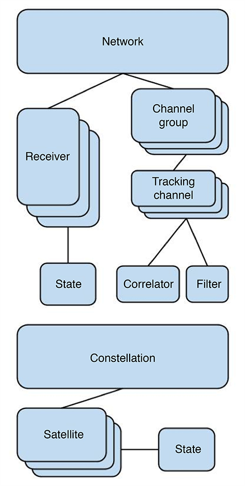
    For data coming from a single real-world receiver, use of the Python Receiver would typically be as follows. First, a user would initialize an instance of the receiver class using a dictionary of predefined settings, such as the file location of the data source. Second, the user would initialize a constellation object of satellites by passing the pseudorandom noise (PRN) code values of each satellite to be included in the constellation. At this point, the user could then use built-in functionality in the receiver object to perform acquisition of all of the satellites in the constellation. Results of this acquisition attempt would be stored in the receiver object, where they could then be used to run the receiver’s built-in scalar tracking functionality. Likewise, scalar tracking data would be stored in the receiver object, and again the user could use the receiver’s built-in navigation functionality to decode the navigation bits produced during scalar tracking and perform navigation computations. Satellite-specific ephemerides would be stored in the relevant satellite objects.

    Navigation solutions are stored as a part of the receiver’s state object. The state object, which is also used in the satellite class, is a container for holding state information in the Earth-centered Earth-fixed (ECEF) coordinate system (such as position and velocity) and clock terms, and it also provides the ability to return position coordinates in other systems, such as the GPS geodetic system (frame) of WGS 84. While it is not a key feature of the Python Receiver, the state object is designed as an object so that it can be readily used elsewhere should an algorithm need to store state information and have coordinate transformations readily available.

    Tracking channels need not be restricted to the hierarchy shown in Figure 1. During operation for just one data source, the scalar tracking function defined at the receiver level will initialize a sufficient number of tracking channels to track all of its observed satellites. However, when operating on multiple sources of data and with the intent to share tracking outputs between channels, it is helpful to place tracking channels into groups, as shown in FIGURE 2. In the example that will be discussed in following sections, two real-world receivers observed a similar set of satellites. It was therefore helpful to define channel groups for each commonly observed satellite, with one channel in the group corresponding to the satellite as tracked by the first receiver, and the other channel corresponding to the satellite as tracked by the second. Tracking groups as a class, however, may be easily modified for other experimental purposes.

    FIGURE 2. Left: an independent tracking channel (corresponding to one tracking channel object). Right: a channel group. Note that in the channel group, updates to the code and carrier phase of each channel may be performed cooperatively.
    FIGURE 2. Left: an independent tracking channel (corresponding to one tracking channel object). Right: a channel group. Note that in the channel group, updates to the code and carrier phase of each channel may be performed cooperatively.

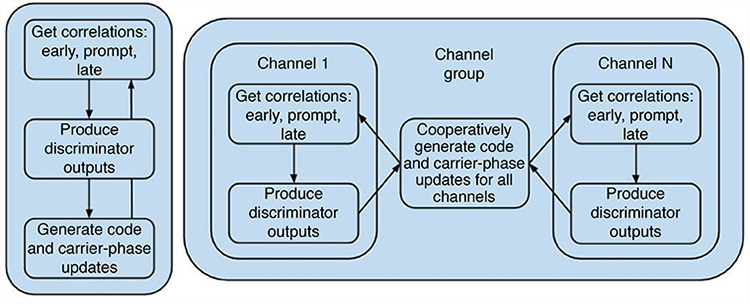
    Independent tracking channels have an update function that processes the next segment of raw data in three main steps: computing correlations (early, late, and prompt), producing discriminator outputs, and generating code and carrier-frequency updates. For a group of channels, this sequence of steps is interrupted after discriminator outputs have been computed. At this point, the channel group may instruct the tracking channels to update their code and carrier frequencies independently or through some other cooperative means that considers data across all of the channels.

    As for the last few classes: correlators and filters are defined as objects so that they can be easily changed depending on the experimental circumstances. And satellites, in addition to holding satellite-specific ephemerides, have built-in functionality to return their locations given a particular epoch of GPS Time.

    Naturally, core functions such as these would be found in traditional software receivers, but by repackaging them into the object-oriented framework, both code reusability and modifiability increase. And in addition, by defining classes for networks of receivers and groups of tracking channels, simulations and experiments involving cooperative positioning of receivers become easier to conduct.

    Experiment

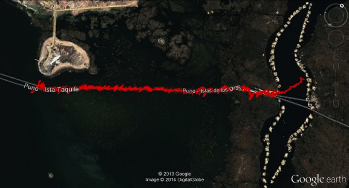
    To help illustrate how the Python Receiver lends itself to the task of cooperatively tracking multiple receivers, concurrent data from two SDR front ends was collected on a boat in Lake Titicaca just offshore from Puno, Peru. The boat was a small motorized ferry capable of transporting approximately twenty passengers. One antenna and front end, hereafter referred to as “Receiver X” was placed on the port side of the boat, while the other, “Receiver Y” was placed on the starboard side. Maintaining a fixed baseline, both receivers captured raw GPS L1 signals from separate portions of the sky and mixed them to an intermediate frequency of 5.456 MHz. Raw data collection was performed concurrently at both receivers for 15 minutes as the boat returned from the floating islands of the Uros people to the dock at Puno. Finally, while Lake Titicaca is at a high elevation in the Altiplano (the Andean Plateau), the surrounding mountains do not rise far above the horizon, and thus visibility was quite good in most directions.

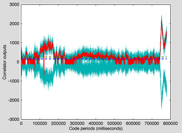
    Some challenges, however, present themselves in this data set. While Receiver X was able to acquire eight satellites, and Receiver Y was able to acquire 10, the signal quality at Receiver Y was generally poor. In Figure 3, in-phase prompt correlator outputs from traditional scalar tracking are shown for both Receivers X and Y and satellites with PRN codes 27 and 29. For satellite 27, Receiver Y loses lock of the signal between code periods 100,000 and 200,000, and for satellite 29, it completely loses track of the signal after only a few thousand code periods. (Recall that the C/A-code period is one millisecond.)

    FIGURE 3. The in-phase prompt correlator outputs for both receivers and satellites PRN 27 and 29. The cyan dots are correlator outputs, the red line is the locking metric, and the dashed green and blue lines are the thresholds set for determining good and poor lock, respectively. Locking metric values above the dashed green line represent a good lock, and values below the dashed blue line represent loss-of-lock. Note that y-axis values differ from graph to graph.
    FIGURE 3. The in-phase prompt correlator outputs for both receivers and satellites PRN 27 and 29. The cyan dots are correlator outputs, the red line is the locking metric, and the dashed green and blue lines are the thresholds set for determining good and poor lock, respectively. Locking metric values above the dashed green line represent a good lock, and values below the dashed blue line represent loss-of-lock. Note that y-axis values differ from graph to graph.

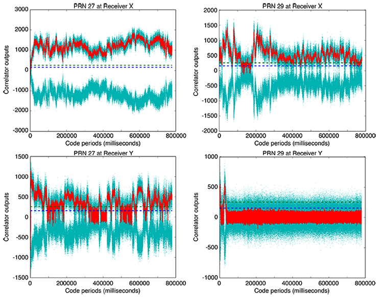
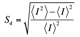
    To better characterize the tracking performance of each receiver-satellite pair, a locking metric was designed and implemented, the values of which are shown as the red lines in the graphs of Figure 3. Inspired by the earlier use of the square-law detector, we have expressed the metric as:

    Python-Eq1(1)

    where N is the number of most recent correlator samples, Ii and Qi are the ith in-phase and quadrature-phase prompt correlator outputs, and the square-root operator returns the negative square root of the absolute value of the expression under the radical if that expression is negative.

    After visually examining the relationship of this locking metric with the quality of the in-phase prompt correlator outputs, two thresholds were determined in order to better characterize the quality of the tracking loop lock. The first threshold, represented as the dashed green lines in the graphs of Figure 3, is the threshold above which the tracking loops were considered locked well. Its value was set to 250. The second threshold, whose value was set to 150 and is represented by the dashed blue lines, is the threshold below which the tracking loops were considered to be in a complete loss-of-lock situation. Locking metric values between 150 and 250 were considered as representing a situation in which the tracking loops were weakly locked to the incoming signals.

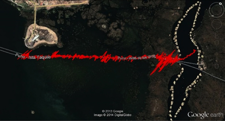
    Despite the poor performance of Receiver Y in tracking many of its signals, navigation functionality in the Python Receiver was still able to recover sufficient ephemerides from the tracking data to perform position calculations. FIGURE 4 shows the navigation solutions for Receiver Y over a 13-minute interval, roughly capturing the route that the ferry took westward back to Puno. Note that the moustache-shaped region in the right-hand side of the map is the collection of floating islands of the Uros. Just as the ferry left these islands, the navigation solutions for Receiver Y become much nosier. Possible reasons for this are the slight change in heading that the ferry made, or the thicket of reeds that surrounded the boat during this portion of the journey. Navigation results for Receiver X were much less noisy.

    FIGURE 4. The trip back to Puno on the left (west) from the floating islands of the Uros on the right (east) as determined by traditional scalar tracking and navigation at Receiver Y. Image courtesy of Google Earth and the GPS Visualizer.
    FIGURE 4. The trip back to Puno on the left (west) from the floating islands of the Uros on the right (east) as determined by traditional scalar tracking and navigation at Receiver Y. Image courtesy of Google Earth and the GPS Visualizer.

    Cooperative Scalar Tracking

    While all of these traditional results were obtained using the Python Receiver, they could have just as easily been obtained using procedurally coded receivers. Assuming, however, that one is interested in performing experiments that involve data sharing between multiple receivers, the Python Receiver lends itself handily to the task.

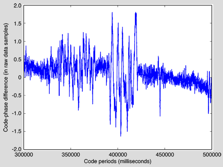
    An experiment was devised in which scalar tracking performed at both Receivers X and Y would be done cooperatively. In particular, it was observed that often when one of the two receivers momentarily lost track of its signal for a particular satellite, the other receiver would be tracking well. In addition, it was noted that because the two receivers maintained a fixed baseline during tracking, their tracking channels should have maintained a steady difference in code phases that changed slowly provided that the receiver-satellite geometry did not change quickly. As shown in FIGURE 5, the only violation of this scenario would occur when one of the two receivers lost lock and thus allowed for drift in its code-tracking loop. It should be noted that unlike the situation in Figure 5, the reported code difference between the two receivers suffered from a bias that grew linearly in time. This bias, which was likely due to clock errors in one or both of the receiver front ends, was eliminated through a linear regression before the plotting of the figure.

    FIGURE 5. The code-phase difference between Receivers X and Y for PRN 27 from 300,000 to 500,000 milliseconds. Note the large variance around 400,000 milliseconds corresponding to a loss-of-lock for Receiver Y.
    FIGURE 5. The code-phase difference between Receivers X and Y for PRN 27 from 300,000 to 500,000 milliseconds. Note the large variance around 400,000 milliseconds corresponding to a loss-of-lock for Receiver Y.

    All of these observations motivated the following cooperative scalar tracking design. First, any satellite that was observed by only one receiver would be independently tracked by that receiver in the traditional manner. A single tracking loop object would be allocated in Python for this particular receiver-satellite pair. Second, any satellite that was observed by both receivers would have a channel group object allocated in Python. This channel group would contain two tracking channel objects, one for each receiver.

    As shown in Figure 2, this channel group required specific code to be written to handle the cooperative updates of both receivers’ code and carrier frequencies. The algorithm was designed as follows. For each update epoch (generated by a call of the channel group’s update function), if both of the tracking channels were locked to their incoming signals, the channel group would save their code-phase difference for that code period. And since both channels were locked, both would update their code and carrier frequencies in the traditional manner, relying on discriminator outputs only.

    If, on the other hand, one of the tracking channels was in a loss-of-lock situation, the channel group would search the previous 5,000 milliseconds of data for code periods during which, presumably, both tracking channels were mutually locked. This data would contain information about the expected code-phase difference between the two tracking channels at the current code period. At this point, a linear regression on the data from the mutually locked code periods was used to determine this expected code-phase difference. Finally, we note again that this expected code-phase difference would only remain valid under the assumption that the receiver-satellite geometry was not changing rapidly, as was the case for this data. But acknowledging that some changes in the geometry might occur (such as a change in heading of the boat) is the reason why the search interval for mutually locked data was limited to five seconds.

    Assuming that one of the receivers was in a loss-of-lock situation and that sufficient data from the past five seconds existed to generate an estimate of the current expected code-phase difference, the channel group could then make a cooperative update of the lockless tracking channel. For this channel, the channel group would replace the traditional code-tracking discriminator outputs with the offset of the expected code-phase difference dexp from the currently observed code-phase difference dcur. In the following equation, the new discriminator output is denoted as c:

    Python-Eq2. (2)

    Expressing dcur=ycurxcur and dexp=yexpxexp, where xcur/exp and ycur/exp represent current and expected code phases at two receivers, we can rewrite Equation 2 as

    Python-Eq3  (3)

    or

    Python-Eq4  (4)

    since we expect the x receiver to be locked, and therefore Python-Eq4-a .

    Some finer points to mention include that the “loss-of-lock” and “tracking well” designations were determined by way of the locking metric defined in the previous section. In addition, if a receiver was “tracking weakly,” it would update its code and carrier frequencies by relying solely on its own discriminator outputs. Also, because in traditional scalar tracking loss-of-lock might occur for an extended interval greater than five seconds at one receiver (such as Receiver Y’s tracking of satellite 27 seen in Figure 3 between 300,000 and 400,000 milliseconds), whenever the channel group was called to cooperatively update a lockless tracking channel’s code frequency, it would record the current code-phase difference between both receivers. Under all scenarios, the carrier-frequency update would be done independently at each channel using discriminator outputs alone. And finally, in order for both receivers to share relevant data with each other during tracking, clock bias terms found after traditional scalar tracking were used to align in time the raw data files for each receiver appropriately.

    Results and Discussion

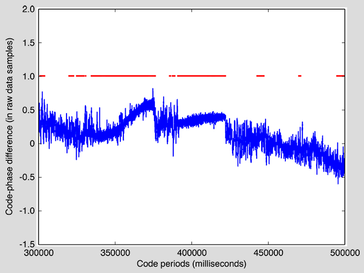
    Using cooperative scalar tracking, drifting of the code-phase difference during code periods when one of the receivers is experiencing loss-of-lock is expected to be suppressed. And indeed, results such as those shown in FIGURE 6 verify this expectation. Since cooperative scalar tracking does not attempt to modify the way either receiver tracks during periods of good lock, this type of modified scalar tracking is not expected to produce less noisy tracking results. It is expected, however, to help lockless tracking channels to regain track after short signal outages, similar to the benefits of vector tracking.

    FIGURE 6. The code-phase difference between Receivers X and Y for PRN 27 from 300,000 to 500,000 milliseconds, this time using cooperative scalar tracking. Presence of the red line indicates code periods during which cooperative code-phase updates were made for Receiver Y. Note that noisy drifting of the code-phase difference is suppressed.
    FIGURE 6. The code-phase difference between Receivers X and Y for PRN 27 from 300,000 to 500,000 milliseconds, this time using cooperative scalar tracking. Presence of the red line indicates code periods during which cooperative code-phase updates were made for Receiver Y. Note that noisy drifting of the code-phase difference is suppressed.

    Strikingly, this form of cooperative tracking allowed for Receiver Y to continually track the signal from satellite 29 (albeit with occasional outages) for the full thirteen minutes of data shown in FIGURE 7. Whereas in Figure 3, Receiver Y very quickly loses track of satellite 29, Figure 7 shows that Receiver Y, under cooperative scalar tracking, can maintain a good enough lock on the signal that by roughly 750,000 code periods, it is able to pick up the signal again quite strongly. This change in signal strength may have been due to a slight change in heading that the ferry made near Isla Taquile towards the end of this data set (see Figure 4 and FIGURE 8).

    FIGURE 7. The in-phase prompt outputs for Receiver Y and PRN 29 using cooperative scalar tracking. Compare this to the bottom-right graph in Figure 3. Inter-receiver aiding allowed Receiver Y to track this signal for a majority of the code periods.
    FIGURE 7. The in-phase prompt outputs for Receiver Y and PRN 29 using cooperative scalar tracking. Compare this to the bottom-right graph in Figure 3. Inter-receiver aiding allowed Receiver Y to track this signal for a majority of the code periods.
    FIGURE 8. The trip back to Puno as determined by Receiver Y after cooperative scalar tracking and navigation computations. Compared to Figure 4, the navigation solutions are less noisy. Image courtesy of Google Earth and the GPS Visualizer.
    FIGURE 8. The trip back to Puno as determined by Receiver Y after cooperative scalar tracking and navigation computations. Compared to Figure 4, the navigation solutions are less noisy. Image courtesy of Google Earth and the GPS Visualizer.

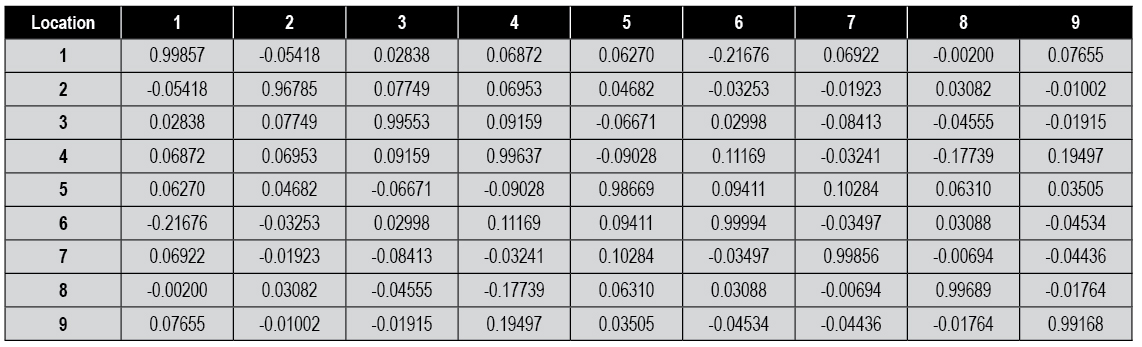
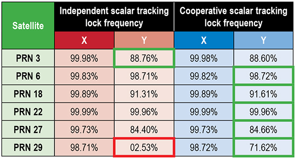
    Given the locking metric defined in the section “Experiment,” quantitative measures of how often each channel spent locked or in loss-of-lock can be made. In total, both receivers tracked six common satellites (with each receiver also tracking other satellites independently). TABLE 1 shows the locking frequencies for each commonly tracked satellite.

    TABLE 1. Percent of time each tracking channel spent locked. Lock was designated if the locking metric was above 150. The best values for Receiver Y are highlighted in green, with the most notable improvement occurring for satellite 29.
    TABLE 1. Percent of time each tracking channel spent locked. Lock was designated if the locking metric was above 150. The best values for Receiver Y are highlighted in green, with the most notable improvement occurring for satellite 29.

    Granted that the drift in the code phase for lockless tracking channels is curtailed in cooperative scalar tracking, an improvement in navigation solutions is also expected. This expectation is verified by comparing the qualitative level of noise in the solutions of Figure 8 to the solutions in Figure 4. Notably, the noise in the reed thicket (the section of the route immediately after leaving the moustache-shaped floating islands region) is suppressed. Not shown are the navigation solutions for the port side receiver, Receiver X, which by comparison to Receiver Y were relatively good in both forms of scalar tracking.

    Conclusion

    The experiment we carried out highlighted the abilities of the Python Receiver. Data from two SDR front ends and associated antennas placed on either side of a small transport ferry was used to track both receivers by using groups of tracking channels that could cooperatively modify their individual channels’ code and carrier frequencies. In this way, loss-of-lock in many of the tracking channels was avoided leading to improved navigation precision. More importantly, it is expected that future experiments like these can be easily implemented within the framework of the Python Receiver, and thus topics like cooperative vector tracking might be more easily investigated.

    Acknowledgments

    This article is based, in part, on the paper “A Python Software Platform for Cooperatively Tracking Multiple GPS Receivers” presented at ION GNSS+ 2014, the 27th International Technical Meeting of the Satellite Division of The Institute of Navigation, held in Tampa, Florida, September 8–12, 2014.

    Manufacturers

    The Python Receiver uses SiGe GN3S v3 Samplers, developed by the University of Colorado and SiGe Semiconductor (acquired by Skyworks Solutions Inc., Woburn, Massachusetts) and marketed by SparkFun Electronics, Niwot, Colorado.


    ELIOT WYCOFF received his B.S. in applied mathematics from Columbia University, New York, in 2011. While working on the Python Receiver, he was a graduate student in the Department of Aerospace Engineering at the University of Illinois at Urbana-Champaign (UIUC).

    YUTING NG obtained a B.S. in electrical and computer engineering from UIUC in 2014. She is currently a graduate student in the Department of Aerospace Engineering, UIUC.

    GRACE XINGXIN GAO is an assistant professor in the Department of Aerospace Engineering, UIUC. She received her B.S. in mechanical engineering in 2001 and her M.S. in electrical engineering in 2003, both from Tsinghua University, China. She obtained her Ph.D. in electrical engineering at Stanford University in 2008. Before joining UIUC in 2012, Gao was a research associate at Stanford University.


    FURTHER READING

    • Authors’ Conference Paper

    A Python Software Platform for Cooperatively Tracking Multiple GPS Receivers” by E. Wycoff and G.X. Gao in Proceedings of ION GNSS+ 2014, the 27th International Technical Meeting of the Satellite Division of The Institute of Navigation, Tampa, Florida, September 8–12, 2014, pp. 1417–1425.

    Software-Defined GNSS Receivers

    Digital Satellite Navigation and Geophysics: A Practical Guide with GNSS Signal Simulator and Receiver Laboratory by I.G. Petrovski and T. Tsujii with foreword by R.B. Langley, published by Cambridge University Press, Cambridge, U.K., 2012.

    Software GNSS Receiver: An Answer for Precise Positioning Research” by T. Pany, N. Falk, B. Riedl, T. Hartmann, G. Stangl, and C. Stöber in GPS World, Vol. 23, No. 9, September 2012, pp. 60–66.

    A Software-Defined GPS and Galileo Receiver: A Single-Frequency Approach by K. Borre, D.M. Akos, N. Bertelsen, P. Rinder, and S.H. Jensen, published by Birkhäuser Engineering, Springer-Verlag GmbH, Heidelberg, 2007.

    GNSS Software Defined Radio: Real Receiver or Just a Tool for Experts?” by J.-H. Won, T. Pany, and G. Hein in Inside GNSS, Vol. 1, No. 5, July–August 2006, pp. 48–56.

    Satellite Navigation Evolution: The Software GNSS Receiver” by G. MacCougan, P.L. Normark, and C. Ståhlberg in GPS World, Vol. 16, No. 1, January 2005, pp. 48–55.

    Python

    Learn Python in One Hour by V.R. Volkman, published by Modern Software Press, L.H. Press Inc., Ann Arbor, Michigan, 2014.

    A Primer on Scientific Programming with Python by H.P. Langtangen, published by Springer-Verlag GmbH, Heidelberg, 2009.

    “Python for Scientific Computing” by T.E. Oliphant in Computing in Science & Engineering, Vol. 9, No. 3, May–June 2007, pp. 10–20, doi: 10.1109/MCSE.2007.58.

    Noncoherent Integration

    GNSS Radio: A System Analysis and Algorithm Development Research Tool for PCs” by J.K. Ray, S.M. Deshpande, R.A. Nayak, and M.E. Cannon in GPS World, Vol. 17, No. 5, May 2006, pp. 51–56.

    Fundamentals of Global Positioning System Receivers: A Software Approach, 2nd edition, by J. B.-Y. Tsui, published by Wiley-Interscience, John Wiley & Sons, Inc., Hoboken, New Jersey, 2005.

    “An Assisted GPS Acquisition Method Using L2 Civil Signal in Weak Signal Environment” by D.J. Cho, C. Park, and S.J. Lee in Journal of Global Positioning Systems, Vol. 3 No. 1-2, December 2004, pp. 25–31.

    GPS Position Display

    GPS Visualizer: Do-It-Yourself Mapping” website by A. Schneider.

    Square Law Detector

    “Lock Detection in Costas Loops” by A. Mileant and S. Hinedi in IEEE Transactions on Communications, Vol. 40, No. 3, March 1992, pp. 480–483, doi: 10.1109/26.135716.

  • Orbit of One Wayward Galileo Satellite Raised

    Orbit of One Wayward Galileo Satellite Raised

    The orbit of one of the two Galileo satellites launched into incorrect orbits on August 22 is being adjusted. Tracking data supplied by the North American Aerospace Defense Command (NORAD) and the U.S. Joint Space Operations Center (JSpOC) has confirmed the change.

    Also, the first navigation signal from Galileo 5 has been received.

    The satellites were supposed to go into circular orbits with an inclination to the equator of 56 degrees and with a semi-major axis of about 29,600 km. They ended up in eccentric orbits with semi-major axes more than 3,300 km shorter and with an inclination of about 49.7 degrees.

    Instead of an orbital height of 23,222 km above the surface of the Earth, they were moving between apogee heights of about 25,900 km and perigee heights of about 13,800 km, perilously close to the most dangerous regions of the Van Allen radiation belts.

    The European Space Agency announced on November 10 that the orbit of one of the two wayward satellites, Galileo 5, would have its perigee raised to 17,339 km through a series of 15 orbital maneuvers. This orbital adjustment would put the satellite into a safer orbit and potentially make it useable for positioning and navigation. If the operation is successful, Galileo 6 will follow suit.

    These maneuvers likely started on or shortly after November 8. After the maneuvers began, NORAD/JSpOC temporarily “lost” the satellite as often happens when satellites undergo unpredicted Delta-V operations. NORAD/JSpOC recovered the satellite after about 18 days and issued new orbital elements for the satellite on November 25.

    The new elements show that (so far) the perigee of Galileo 5 has been raised from about 13,820 km to 17,230 km with a corresponding change in the orbital eccentricity from about 0.23053 to 0.15619. The apogee height is virtually the same as that immediately after launch. Also, the inclination is not and will not be materially changed.

    An animation, produced using the NORAD/JSpOC orbital element sets and the XEphem software, compares Galileo 5’s old and new orbits:

  • Innovation: A Bright Idea

    Innovation: A Bright Idea

    Testing the Feasibility of Positioning Using Ambient Light

    By Jingbin Liu, Ruizhi Chen, Yuwei Chen, Jian Tang, and Juha Hyyppä

    INNOVATION INSIGHTS by Richard Langley
    INNOVATION INSIGHTS by Richard Langley

    AND THEN THERE WAS LIGHT. Well, the whole electromagnetic (EM) spectrum, actually. Visible light occupies only a small portion of the spectrum, which extends from below the extremely low frequency (ELF) 3 to 30 hertz band with equivalent wavelengths of 100,000 to 10,000 kilometers through infrared, visible, and ultraviolet light and x-rays to gamma rays in the 30 to 300 exahertz band (an exahertz is 1018 hertz) with wavelengths of 10 to 1 picometers and beyond. The radio part of the spectrum extends to frequencies of about 300 gigahertz or so, but the distinction between millimeter radio waves and long infrared light waves is a little blurry.

    Natural processes can generate electromagnetic radiation in virtually every part of the spectrum. For example, lightning produces ELF radio waves, and the black hole at the center of our Milky Way Galaxy produces gamma rays. And various mechanical processes can be used to generate and detect EM radiation for different purposes from ELF waves for communication tests with submerged submarines to gamma rays for diagnostic imaging in nuclear medicine.

    Various parts of the EM spectrum have been used for navigation systems over the years. For example, the Omega system used eight powerful terrestrial beacons transmitting signals in the range of 10 to 14 kilohertz permitting global navigation on land, in the air, and at sea. At the other end of the spectrum, researchers have explored the feasibility of determining spacecraft time and position using x-rays generated by pulsars — rapidly rotating neutron stars that generate pulses of EM radiation.

    But the oldest navigation aids, lighthouses, used the visible part of the EM spectrum. The first lighthouses were likely constructed by the ancient Greeks sometime before the third century B.C. The famous Pharos of Alexandria dates from that era. And before the construction of lighthouses, mariners used fires built on hilltops to help them navigate. The Greeks also navigated using the light from stars, or celestial navigation.  Records go back to Homer’s Odyssey where we read “Calypso, the lovely goddess had told him to keep that constellation [the Great Bear] to port as he crossed the waters.” By around 1500 A.D., the astrolabe and the cross-staff had been developed sufficiently that they could be used to measure the altitudes of the sun or stars to determine latitude at sea. Celestial navigation was further advanced with the introduction of the quadrant and then the sextant. And determining longitude was possible by observing the moons of Jupiter (but not easily done at sea), measuring distances between the moon and other celestial bodies and, once it was developed, using a chronometer to time altitude observations.

    How else is light used for positioning and navigation? Early in the space age, satellites were launched with flashing beacons or with large surface areas to reflect sunlight so that they could be photographed from the ground against background stars with known positions to determine the location of the camera. We also have laser ranging to satellites and the moon and the related terrestrial LiDAR technology, as well as the total stations used by surveyors. And in this month’s column, we take a look at the simple, innovative method of light fingerprinting: the use of observations of the artificial light emitted by unmodified light fixtures as well as the natural light that passes through windows and doorways in a technique for position determination inside buildings.


    “Innovation” is a regular feature that discusses advances in GPS technology and its applications as well as the fundamentals of GPS positioning. The column is coordinated by Richard Langley of the Department of Geodesy and Geomatics Engineering, University of New Brunswick. He welcomes comments and topic ideas.


    Over the years, various localization technologies have been used to determine locations of people and devices in an absolute or relative sense. Relative positioning methods determine a location relative to another one in a local coordinate framework, while absolute positioning techniques fix an absolute location in a specific coordinate framework.

    In the past, people observed the positions (orientation angles) of a celestial body (such as the sun, the moon, or a star) to determine their locations on the Earth, which is known as celestial navigation (see FIGURE 1). The locations are resolved by relating a measured angle between the celestial body and the visible horizon to the Nautical Almanac, which is a knowledge base containing the coordinates of navigational celestial bodies and other relevant data. Other than an observation device, celestial navigation does not rely on any infrastructure, and hence it can be used virtually anywhere on the globe at anytime, weather permitting. Nowadays, an increasing number of applications, location-based services, and ambient intelligence largely require positioning functions across various environments due to increasing mobility of people and devices. In particular, the development of robotics for a number of purposes requires the support of localization capability in various conditions where positioning infrastructure may be missing.

    Various positioning technologies share an intrinsic characteristic that a positioning solution is resolved by using the dependency between spatial locations and a set of physical observables. The dependency may be expressed in the form of either a deterministic function model or a probabilistic model. A deterministic model expresses the dependency between locations and observables in a closed-form function, while a probabilistic model defines the dependency between locations and observables in the Bayesian sense. Depending on the form of dependency, different mathematical models have been used for position resolution.  

    For example, satellite-based GNSS positioning derives the location of a user’s receiver based on radio frequency (RF) signals transmitted by the satellite systems. GNSS positioning is grounded in accurate time determination: the time differences between the transmitted and the received radio signals denote signal travel times (observables), which are then converted into distance measurements between the satellite and the user antenna. Using the distance measurements between the user antenna and four different satellites, the receiver can obtain three-dimensional receiver coordinates in a global reference frame and the time difference between the receiver and satellite clocks. The dependency between user location and a set of distance observables can be expressed in a simplified equation:

    Inn-Eq-1(1)

    where ρi is an observed range between the ith satellite and the receiver, (x,y,z)i is the position of the ith satellite, (x,y,z) is the position of the receiver to be estimated, γ denotes errors in the range observable, δt and c are receiver clock error and the speed of  light, respectively (the sign of the clock term is arbitrary, but must be used consistently).

    It is obvious that GNSS positioning relies strongly on the visibility of the GNSS constellation — the space infrastructure — as it requires line-of-sight visibility of four or more satellites. The positioning capability is degraded or totally unavailable in signal-blocked environments, such as indoors and in urban canyons. 

    An example of Bayesian positioning is to use various signals of opportunity (SOOP) — signals not originally intended for positioning and navigation. They include RF signals, such as those of cellular telephone networks, digital television, frequency modulation broadcasting, wireless local area networks, and Bluetooth, as well as naturally occurring signals such as the Earth’s magnetic field and the polarized light from the sun. Indicators of these signals, such as signal strengths and signal quality, are dependent on locations in the Bayesian sense. The dependency between signal indicators and locations is expressed in a probabilistic model:

    Inn-Eq-2  (2)

    where  signifies a dependency between a set of physical signals and locations, I denotes indicators of SOOP signals, L denotes location, and P(i|l) is the probability that signal indicators (i) are observed at location (l).

    Positioning resolution involves finding a location that yields the maximum a posteriori probability given a specific set of observables. Bayes’ Rule for computing conditional probabilities is applicable in the positioning estimation, and a family of Bayesian inference methods has been developed (see Further Reading). 

    An inertial navigation system (INS) is a typical relative positioning technology, and it provides the estimation of moved distance, direction, and/or direction change. A commonly used INS consists of accelerometers, gyroscopes, and a compass. It is self-contained and needs no infrastructure in principle to operate. However, the sensors yield accumulated positioning errors, and they need extra information for calibration. For example, in a GNSS/INS combined system, the INS needs to be calibrated using GNSS positioning results. To achieve an enhanced positioning performance in terms of availability, accuracy, and reliability, different positioning technologies are commonly integrated to overcome the limitations of individual technologies in applicability and performance.

    This article discusses the feasibility of ambient light (ambilight) positioning, and we believe it is the first time that ambilight has been proposed as a positioning signal source. We propose the use of two types of observables of ambient light, and correspondingly two different positioning principles are applied in the positioning resolution. Our solution does not require any modifications to commonly used sources of illumination, and it is therefore different from other indoor lighting positioning systems that have been proposed, which use a modulated lighting source.

    Ambilight positioning does not require extra infrastructure because illumination infrastructure, including lamps and their power supply and windows, are always necessary for our normal functioning within spaces. Ambilight exists anywhere (indoor and outdoor), anytime, if we consider darkness as a special status of ambient light. Ambilight sensors have been sufficiently miniaturized and are commonly used. For example, an ambilight sensor is used in a modern smartphone to detect the light brightness of the environment and to adaptively adjust the backlight, which improves the user vision experience and conserves power. Additionally, ambilight sensors are also widely used in automotive systems to detect the light intensity of environments for safety reasons. Therefore, ambilight positioning can use existing sensors in mobile platforms. This article presents the possibilities and methods of ambilight positioning to resolve both absolute and relative positioning solutions, and which can be integrated as a component in a hybrid positioning system. 

    Absolute Positioning Using Ambilight Spectral Measurements 

    The essence of localization problems is to resolve the intrinsic dependency of location on a set of physical observables. Therefore, a straightforward idea is that the type of observables applicable to positioning can be determined once the location-observables dependency is established. The feasibility is validated when the location-observables dependency is confirmed in the sense of necessary and sufficient conditions.

    Ambient light is a synthesis of artificial light sources and natural light. The light spectrum is defined by the distribution of lighting intensity over a particular wavelength range. Researchers have reported development of sensor technology that has a spectral response from 300 to 1450 nanometers (from ultraviolet through infrared light). The spectrum of ambient light is mainly determined by colors of reflective surfaces in the circumstance, in addition to that of artificial and natural light sources. Therefore, intensity spectrum measurements are strongly correlated with surrounding environments of different locations. The traditional fingerprinting method can be used to resolve the positioning solution. 

    The fingerprinting approach makes use of the physical dependency between observables and geo-locations to infer positions where signals are observed. This approach requires the knowledge of observable-location dependency, which comprises a knowledge database. The fingerprinting approach resolves the most likely position estimate by correlating observed SOOP measurements with the knowledge database. The related fingerprinting algorithms include K-nearest neighbors, maximum likelihood estimation, probabilistic inference, and pattern-recognition techniques. These algorithms commonly consider moving positions as a series of isolated points, and they are therefore related to the single-point positioning approach. In addition, a “hidden Markov” model method has been developed to fuse SOOP measurements and microelectromechanical systems (MEMS) sensors-derived motion-dynamics information to improve positioning accuracy and robustness.

    In the case of ambilight positioning, prior knowledge is related to structure layout information, including the layout of a specific space, spatial distribution of lighting sources (lamps), types of lighting sources, and windows and doors where natural light can come through. Spatial distribution of lighting sources is normally set up together with power supplies when the structure is constructed, and their layout and locations are not usually changed thereafter. For example, illumination lamps are usually installed on a ceiling or a wall in fixed positions, and the locations of doors and windows, through which light comes, are also typically fixed throughout the life of a building. Therefore, the knowledge database of lighting conditions can be built up and maintained easily through the whole life cycle of a structure.

    In practice, a specific working region is divided into discrete grids, and intensity spectrum measurements are collected at grid points to construct a knowledge database. The grid size is determined based on the required spatial resolution and spatial correlation of spectrum measurements. The spatial correlation defines the degree of cross-correlation of two sets of spectrum measurements observed at two separated locations.

    We measured the spectrum of ambient light with a two-meter grid size in our library. The measurements were conducted using a handheld spectrometer. FIGURE 2 shows a set of samples of ambilight spectrum measurements, and the corresponding photos show the circumstances under which each spectrum plot was collected. These spectral measurements show strong geo-location dependency. Spectrum differences of different locations are sufficiently identifiable. TABLE 1 shows the cross-correlation coefficients of spectral measurements of different locations. The auto-correlation coefficients of spectral measurements of a specific location are very close to the theoretical peak value of unity, and the cross-correlation coefficients of spectra at different locations are significantly low. Therefore, the correlation coefficient is an efficient measure to match a spectrum observable with a geo-referred database of ambilight spectra.

    FIGURE 2. Ambilight spectral measurements of nine locations in the library of the Finnish Geodetic Institute (arbitrary units). The photos below the spectrum plots show the circumstances under which the corresponding spectral measurements were collected.
    FIGURE 2. Ambilight spectral measurements of nine locations in the library of the Finnish Geodetic Institute (arbitrary units). The photos below the spectrum plots show the circumstances under which the corresponding spectral measurements were collected.
    TABLE 1. Correlation coefficient matrix of spectral measurements of different locations.
    TABLE 1. Correlation coefficient matrix of spectral measurements of different locations.

    Relative Positioning Using Ambilight Intensity Measurements

    Total ambilight intensity is an integrated measure of the light spectrum, and it represents the total irradiance of ambient light. In general, a lamp produces a certain amount of light, measured in lumens. This light falls on surfaces with a density that is measured in foot-candles or lux. A person looking at the scene sees different areas of his or her visual field in terms of levels of brightness, or luminance, measured in candelas per square meter. The ambilight intensity can be measured by a light detector resistor (LDR), and it is the output of an onboard 10-bit analog-to-digital converter (ADC) on an iRobot platform, which is the platform for a low-cost home-cleaning robot as shown in FIGURE 3.

    FIGURE 3. The iRobot-based multi-sensor positioning platform, which is equipped with a light sensor and other versatile positioning sensors as marked in the figure.
    FIGURE 3. The iRobot-based multi-sensor positioning platform, which is equipped with a light sensor and other versatile positioning sensors as marked in the figure.

    We designed a simple current-to-voltage circuit based on an LDR and a 10-kilohm resistor, and the integrated analog voltage is input into the iRobot’s ADC with a 25-pin D-type socket, which is called the Cargo Bay Connector. FIGURES 4 and 6 show that the LDR sensor was not saturated during the test whenever we turned the corridor lamps on or off. Since the output of the light sensor was not calibrated with any standard light source, the raw ADC output rather than real values of physical light intensity was used in this study. During the test, the iRobot platform ran at a roughly constant speed of 25 centimeters per second, and the response time of the LDR was 50 milliseconds according to the sensor datasheet. The sampling rate of light intensity measurements was 5 Hz. Thus, the ADC could digitalize the input voltage in a timely fashion.

    FIGURE 4. Total irradiance intensity measurements of ambient light in a closed space. The estimated lamp positions (magenta points) can be compared to the true lamp positions (green points).
    FIGURE 4. Total irradiance intensity measurements of ambient light in a closed space. The estimated lamp positions (magenta points) can be compared to the true lamp positions (green points).
    FIGURE 6. Total irradiance intensity measurements of ambient light in the open corridor of the third floor.
    FIGURE 6. Total irradiance intensity measurements of ambient light in the open corridor of the third floor.

    We conducted the experiments with the iRobot platform in two corridors in the Finnish Geodetic Institute building. The robot was controlled to move along the corridors, and it collected measurements as it traveled. The two corridors represent two types of environment. The corridor of the first floor is a closed space where there is no natural light, and the corridor of the third floor has both natural light and artificial illuminating light. The illuminating fluorescent lamps are installed in the ceiling. In a specific environment, fluorescent lamps are usually installed at fixed locations, and their locations are not normally changed after installation. Therefore, the knowledge of lamp locations can be used for positioning.

    Ambilight positioning is relatively simple in the first case where there is no natural light in the environment and all ambilight intensity comes from artificial light. Because the fluorescent lamps are separated by certain distances, the intensity measurements have a sine-like pattern with respect to the horizontal distance along the corridor. The sine-like pattern is a key indicator to be used for detecting the proximity of a lamp. As shown in Figures 4 and 6, raw measurements of ambilight intensity and smoothed intensity have a sine-like pattern. Because raw intensity measurements have low noise, either raw measurements or smoothed intensity can be used to detect the proximity of a lamp. Figure 4 also shows the results of detection and the comparison to the true lamp positions. There are four fluorescent lamps in this corridor test. The first three were detected successfully, and the estimated positions are close to true positions with a root-mean-square (RMS) error of 0.23 meters. The fourth lamp could not be detected because its light is blocked by a shelf placed in the corridor just below the lamp as shown in FIGURE 5. Figure 4 shows the sine-like intensity pattern of the fourth lamp did not occur due to the blockage.

    FIGURE 5. The light of the fourth lamp in the corridor is blocked by shelves, and the corresponding sine-like light pattern does not appear.
    FIGURE 5. The light of the fourth lamp in the corridor is blocked by shelves, and the corresponding sine-like light pattern does not appear.

    On the third floor, the situation is more complicated because there is both natural light and incandescent lamps in the corridor. Natural light may come in from windows, which are located at multiple locations on the floor. In addition, the light spectrum in the corridor may be interfered with by light from office rooms around the floor. To recover the sine-like intensity pattern of the lamps, the intensity of the background light was measured when the incandescent lamps were turned off. Therefore, the calibrated intensity measurements of illuminating lamps can be calculated as follows:

    Inn-Eq-3  (3)

    where Ia is the intensity measurements of composite ambient light, Ib is the intensity measurements of background light, and Ic is the intensity measurements of the calibrated ambient light of the illuminating lamps.

    Figure 6 shows the intensity measurements of composite ambient light, background light, and calibrated lamp light. In addition, the intensity measurements of calibrated lamp light are smoothed by an adaptive low-pass filter to mitigate noise and interference. The intensity measurements of smoothed lamp light were used to estimate the positions of the lamps according to the sine-like pattern. The estimated lamp positions were compared to the true lamp positions, and the errors are shown in FIGURE 7. The estimated lamp positions have a mean error of 0.03 meters and an RMS error of 0.79 meters. In addition, for the total of 15 lamps in the corridor, only one lamp failed to be detected (omission error rate = 1/15) and one lamp was detected twice (commission error rate = 1/15). 

    Discussion and Conclusion

    Ambilight positioning needs no particular infrastructure, and therefore it does not have the problem of infrastructure availability, which many other positioning technologies have, limiting their applicability. For example, indoor positioning systems using Wi-Fi or Bluetooth could not work in emergency cases when the power supply of these devices is cut off. What ambilight positioning needs is just the knowledge of indoor structure and ambilight observables. The lighting conditions of an indoor structure can be reconstructed based on the knowledge of the layout structure whenever illuminating lamps are on or off. Thus, ambilight observables can be related to the layout structure to resolve positioning estimates as we showed in this article. 

    Besides indoor environments, the methods we have presented are also applicable in many other GNSS-denied environments, such as underground spaces and long tunnels. For example, the Channel Tunnel between England and France has a length of 50.5 kilometers, and position determination is still needed in this kind of environment. In such environments, there is usually no natural light, and the intensity of illuminating lamps has a clear sine-like pattern.

    In particular, ambient light positioning is promising for robot applications when a robot is operated for tasks in a dangerous environment where there is no infrastructure for other technical systems such as Wi-Fi networks. Given the knowledge of the lighting infrastructure acquired from the construction layout design, the method of ambilight positioning can be used for robot localization and navigation. Our tests have shown also that the proposed ambilight positioning methods work well with both fluorescent lamps and incandescent lamps, as long as the light intensity sensor is not saturated. 

    A clear advantage of the technique is that the illuminating infrastructure and the structure layout of these environments are kept mostly unchanged during their life cycle, and the lighting knowledge can be constructed from the structure design. Hence, it is easy to acquire and maintain these knowledge bases. The hardware of ambient light sensors is low-cost and miniature in size, and the sensors can be easily integrated with other sensors and systems.

    Although a spectrometer sensor is not currently able to be equipped with a mobile-phone device, the proposed ambilight positioning techniques can still be implemented with a modern mobile phone in several ways. For example, an economical way would be to form a multispectral camera using a selection of optical filters of selected bands or a miniature adjustable gradual optical filter. The spectral resolution then is defined by the bandwidth of the band-pass optical filters and the optical characteristics of the gradual optical filter. Other sensors, such as an acousto-optic tunable filter spectrometer and a MEMS-based Fabry-Pérot spectrometer, could also be used to measure the spectrum of ambilight in the near future. With such techniques, ambilight spectral measurements can be observed in an automated way and with higher temporal resolution. 

    Acknowledgments

    The work described in this article was supported, in part, by the Finnish Centre of Excellence in Laser Scanning Research (CoE-LaSR), which is designated by the Academy of Finland as project 272195. This article is based on the authors’ paper “The Uses of Ambient Light for Ubiquitous Positioning” presented at PLANS 2014, the Institute of Electrical and Electronics Engineers / Institute of Navigation Position, Location and Navigation Symposium held in Monterey, California, May 5–8, 2014.


    JINGBIN LIU is a senior fellow in the Department of Remote Sensing and Photogrammetry of the Finnish Geodetic Institute (FGI) in Helsinki. He is also a staff member of the Centre of Excellence in Laser Scanning Research of the Academy of Finland. Liu received his bachelor’s (2001), master’s (2004), and doctoral (2008) degrees in geodesy from Wuhan University, China. Liu has investigated positioning and geo-reference science and technology for more than ten years in both industrial and academic organizations. 

    RUIZHI CHEN holds an endowed chair and is a professor at the Conrad Blucher Institute for Surveying and Science, Texas A&M University in Corpus Christie. He was awarded a Ph.D. degree in geophysics, an M.Sc. degree in computer science, and a B.Sc. degree in surveying engineering. His research results, in the area of 3D smartphone navigation and location-based services, have been published twice as cover stories in GPS World. He was formerly an FGI staff member.

    YUWEI CHEN is a research manager in the Department of Remote Sensing and Photogrammetry at FGI. His research interests include laser scanning, ubiquitous LiDAR mapping, hyperspectral LiDAR, seamless indoor/outdoor positioning, intelligent location algorithms for fusing multiple/emerging sensors, and satellite navigation.

    JIAN TANG is an assistant professor at the GNSS Research Center, Wuhan University, China, and also a senior research scientist at FGI. He received his Ph.D. degree in remote sensing from Wuhan University in 2008 and focuses his research interests on indoor positioning and mapping.

    JUHA HYYPPA is a professor and the head of the Department of Remote Sensing and Photogrammetry at FGI and also the director of the Centre of Excellence in Laser Scanning Research. His research is focused on laser scanning systems, their performance, and new applications, especially those related to mobile laser scanning and point-cloud processing.


    FURTHER READING

    • Authors’ Conference Paper

    “The Uses of Ambient Light for Ubiquitous Positioning” by J. Liu, Y. Chen, A. Jaakkola, T. Hakala, J. Hyyppä, L. Chen, R. Chen, J. Tang, and H. Hyyppä in Proceedings of PLANS 2014, the Institute of Electrical and Electronics Engineers / Institute of Navigation Position, Location and Navigation Symposium, Monterey, California, May 5–8, 2014, pp. 102–108, doi: 10.1109/PLANS.2014. 6851363.

    • Light Sensor Technology

    “High-Detectivity Polymer Photodetectors with Spectral Response from 300 nm to 1450 nm” by X. Gong, M. Tong, Y. Xia, W. Cai, J.S. Moon, Y. Cao, G. Yu, C.-L. Shieh, B. Nilsson, and A.J. Heeger in Science, Vol. 325, No. 5948, September 25, 2009, pp. 1665–1667, doi: 10.1126/science.1176706.

    • Light Measurement

    “Light Intensity Measurement” by T. Kranjc in Proceedings of SPIE—The International Society for Optical Engineering (formerly Society of Photo-Optical Instrumentation Engineers), Vol. 6307, Unconventional Imaging II, 63070Q, September 7, 2006, doi:10.1117/12.681721.

    • Modulated Light Positioning

    “Towards a Practical Indoor Lighting Positioning System” by A. Arafa, R. Klukas, J.F. Holzman, and X. Jin in Proceedings of ION GNSS 2012, the 25th International Technical Meeting of the Satellite Division of The Institute of Navigation, Nashville, Tennessee, September 17–21, 2012, pp. 2450–2453.

    • Application of Hidden Markov Model Method

    “iParking: An Intelligent Indoor Location-Based Smartphone Parking Service” by J. Liu, R. Chen, Y. Chen, L. Pei, and L. Chen in Sensors, Vol. 12, No. 11, 2012, pp. 14612-14629, doi: 10.3390/s121114612.

    • Application of Bayesian Inference

    “A Hybrid Smartphone Indoor Positioning Solution for Mobile LBS” by J. Liu, R. Chen, L. Pei, R. Guinness, and H. Kuusniemi in Sensors, Vol. 12, No. 12, pp. 17208–17233, 2012, doi:10.3390/s121217208.

    • Ubiquitous Positioning

    Getting Closer to Everywhere: Accurately Tracking Smartphones Indoors” by R. Faragher and R. Harle in GPS World, Vol. 24, No. 10, October 2013, pp. 43–49.

    “Hybrid Positioning with Smartphones” by J. Liu in Ubiquitous Positioning and Mobile Location-Based Services in Smart Phones, edited by R. Chen, published by IGI Global, Hershey, Pennsylvania, 2012, pp. 159–194.

    “Non-GPS Navigation for Security Personnel and First Responders” by L. Ojeda and J. Borenstein in Journal of Navigation, Vol. 60, No. 3, September 2007, pp. 391–407, doi: 10.1017/S0373463307004286.

  • Innovation: Scintillating Statistics

    Innovation: Scintillating Statistics

    A Look at High-Latitude and Equatorial Ionospheric Disturbances of GPS Signals

    By Yu Jiao, Yu (Jade) Morton, Steve Taylor, and Wouter Pelgrum

    INNOVATION INSIGHTS by Richard Langley
    INNOVATION INSIGHTS by Richard Langley

    THE EARTH’S IONOSPHERE. It’s both a blessing and a curse. Together with the magnetosphere, it helps to protect life on our planet from the damaging outpour of particle and electromagnetic radiation from the sun. In particular, it absorbs a lot of the extreme-ultraviolet (EUV) radiation arriving at the Earth. In fact, that is primarily how the ionosphere is formed. The EUV energy strips off the outer electrons of atmospheric gases producing a plasma of free electrons and ions.

    The ionosphere has another beneficial role in that it permits long distance radio communication using high-frequency (HF) or shortwave signals. Although its use is in decline since the advent of the Internet, HF is still in use by some broadcasters and military organizations and is indispensible during natural disasters when electricity grids and network links go down.

    But the ionosphere can be a pain, too, particularly for GNSS users. The signals from GNSS satellites must travel though the ionosphere on their way to receivers on or near the Earth’s surface. The signals are perturbed by the presence of the free electrons causing an advance in the phase of a signal’s carrier and a delay in the arrival of the pseudorandom noise code modulation (due to the refractive index being frequency dependent or dispersive) and so there is a contribution to carrier-phase and pseudorange (code) measurements, which must be accounted for when determining positions, velocities, and time (PVT) from the measurements.

    Again, since the ionosphere is a dispersive medium, by linearly combining simultaneous measurements (either pseudoranges or carrier phases) on two frequencies such as the GPS L1 and L2 frequencies, an observable virtually free of ionospheric effects can be constructed and used for PVT determinations. This approach does require, however, a dual- or multi-frequency receiver. Single-frequency receivers (or the post-processing of single-frequency data) require the use of a model to account for the ionospheric biases as much as possible. The GPS navigation message, for example, includes values of the parameters of a simple ionospheric model. But, on average, its accuracy is only around 50%. More accurate ionospheric corrections can be acquired from elsewhere, even in real time, such as those from satellite-based augmentation systems.

    But there is another ionospheric effect that can play havoc with GNSS signals: scintillations. These are rapid fluctuations in the amplitude and phase of the signals caused by small-scale irregularities in the ionosphere. When sufficiently strong, scintillations can result in the strength of a received signal dropping below the threshold required for acquisition and tracking or in causing problems for the receiver’s phase lock loop resulting in many cycle slips.

    The occurrence of scintillations depends on many factors including solar and geomagnetic activity, time of year, time of day, and geographical location. In particular, scintillations are most prevalent in equatorial and polar (Arctic and Antarctic) regions. And the processes involved are not fully understood, hindering our ability to model and predict scintillations.

    In an effort to help improve the monitoring, mapping, and modeling of scintillations, a team of researchers led by Prof. Jade Morton is monitoring high-latitude and equatorial scintillations and they discuss some of their preliminary results in this month’s column.


    “Innovation” is a regular feature that discusses advances in GPS technology and its applications as well as the fundamentals of GPS positioning. The column is coordinated by Richard Langley of the Department of Geodesy and Geomatics Engineering, University of New Brunswick. He welcomes comments and topic ideas. Write to him at lang @ unb.ca.


    Among other effects of the Earth’s ionosphere on GPS and other GNSS signals, scintillation is potentially the most problematic. Ionospheric scintillation refers to the random amplitude and phase fluctuations of radio signals after propagating through plasma irregularities. These irregularities occur more frequently in high-latitude and equatorial regions, especially during solar maxima. Occurrence of scintillation is difficult to predict and model because of the complexity of the ionosphere’s internal mechanisms and solar activities that are the driving forces of space weather phenomena. GNSS signals are particularly vulnerable to scintillation, as strong scintillation can severely impact the acquisition and tracking processes in GNSS receivers, causing degradation in positioning accuracy and even loss-of-lock. With the increasing reliance on GNSS applications, understanding the characteristics of ionospheric scintillation and its effects on GNSS signals and receivers has become an important topic and has gained worldwide attention from both ionospheric scientists and GNSS engineers.

    Since 2009, our research group has established several ionospheric scintillation monitoring and data collection systems located in high-latitude and equatorial regions. The results presented here are based on data collected from a specialized commercial dual-frequency GPS ionospheric monitoring receiver at Gakona, Alaska (62.4°N, 145.2°W), and a commercial multi-system, multi-frequency GNSS ionospheric monitoring receiver located at Jicamarca, Peru (11.9°S, 76.9°W). 

    Measurements are filtered to remove slowly varying trends caused by satellite-receiver dynamics, receiver oscillator errors, the background ionosphere and troposphere gradient, and other potential contributions from multipath and man-made interferences. Scintillation events above preset threshold levels from the filter outputs are extracted for analysis. The threshold levels are set based on two commonly used scintillation indices, the S4 index and σφ , which are defined as the standard deviations of the detrended signal amplitude and carrier phase to represent the magnitude of signal intensity and phase fluctuation, respectively. In the study discussed in this article, the thresholds for S4 and σφ  are 0.15 and 15°, respectively for high-latitude measurements. For low-latitude data, the threshold for S4 is raised to 0.2 to accommodate stronger amplitude scintillation, while the threshold for σφ remains 15°.

    From data collected at Gakona, between August 2010 and March 2013, we extracted 655 amplitude and 2,355 phase-scintillation events from 657 equivalent days of data, while from data collected at Jicamarca, we extracted about 830 amplitude and 1,100 phase-scintillation events from 190 days of data collected from November 2012 to June 2013. Based on these events, we established a number of amplitude and phase scintillation distributions, which include scintillation-index-magnitude distributions, event-duration distributions, and event-occurrence frequency distributions. These results show very different characteristics of scintillation observed at low latitudes and high latitudes, indicating that there must be different mechanisms contributing to the formation and evolution of ionosphere plasma irregularities in the two regions. These characteristics are useful for scintillation-event prediction and modeling in the future.

    Data Collection System and Event Thresholds

    FIGURE 1 illustrates the general architecture of the event-driven GNSS data collection system. The system hardware consists of a multi-band GNSS antenna, a commercial ionospheric scintillation monitor (ISM) receiver, an array of reconfigurable software-defined radio (SDR) radio-frequency (RF) front-end devices capable of sampling intermediate-frequency (IF) signals, one or multiple data collection servers, a data storage array, timing signal distribution hardware to ensure both time and frequency consistency across all RF front ends and receivers, and network/communication devices that allow remote access of the receivers and servers to monitor the status of the hardware, to query recorded data, and reset and reconfigure the data collection system. 

    FIGURE 1. General architecture of the event-driven GNSS data collection system deployed at several high-latitude and equatorial sites since 2009.
    FIGURE 1. General architecture of the event-driven GNSS data collection system deployed at several high-latitude and equatorial sites since 2009.

    Custom-designed space weather event monitoring and trigger software resides on the data collection and control server. The ISM receiver operates continuously to produce and record routine measurements such as I and Q channel accumulator outputs, pseudorange, carrier phase, Doppler frequency, C/N0, and scintillation indices, while the SDR RF front ends only temporarily store the latest one-minute worth of IF samples in each device’s circular buffer. Scintillation event thresholds are pre-determined based on analysis of baseline data collected at the same local site using the same hardware. The real-time event trigger software compares ISM receiver measurements with the pre-set event threshold. If the measurements exceed the thresholds, the contents of the circular buffers will be written to the data storage array until after the event subsides. These raw IF samples are then further post-processed using a wide range of receiver processing algorithms for analysis of scintillation features and robust receiver algorithm development.

    The high-latitude GNSS receiver array at Gakona, was initially established in 2009 and has been continuously evolving into a four-antenna array capable of collecting GPS L1, L2C, and L5 and GLONASS L1 and L2 signal data until its recent relocation to and upgrade at Poker Flat Research Range, north of Fairbanks. Several publications have discussed the system setup, receiver signal processing of data collected by the system, and characterization of high-latitude scintillations based on analysis of the array outputs (see Further Reading). In this article, only the data collected using the commercial ISM receiver are discussed because this is the longest operating receiver at this site. The receiver outputs L1C/A signal intensity and carrier-phase measurements at a rate of 50 Hz and semi-codeless tracking results of L2P(Y) at 1 Hz.

    Since 2011, several GNSS data collection systems have been deployed at low-latitude locations, including Hong Kong, Singapore, Peru, Ascension Island, and Puerto Rico. In this article, we use results from the ISM receiver at Jicamarca, Peru, close to the geomagnetic equator. FIGURE 2 shows the data-collection-system-setup block diagram at Jicamarca. The ISM receiver used in this location generates 100-Hz carrier-phase measurements and I/Q channel correlator outputs; the latter are further processed to generate 50-Hz signal-intensity measurements for GPS L1C/A, L2C, and L5 signals and GLONASS, Galileo, and BeiDou open signals. Seven SDR front ends driven by the same oven-controlled crystal oscillator (OCXO) signal from the ISM receiver sample GPS, GLONASS, Galileo, and BeiDou open signals. Preliminary results obtained from these and other low-latitude SDR data have been presented in several papers in the archived literature (see Further Reading). 

    FIGURE 2. Current multi-GNSS data collection system configuration at Jicamarca Radio Observatory in Peru. (GLO = GLONASS, BDS = BeiDou System, VPN = virtual private network, ISMET = ionospheric scintillation monitoring event triggering, RAID = redundant array of independent disks)
    FIGURE 2. Current multi-GNSS data collection system configuration at Jicamarca Radio Observatory in Peru. (GLO = GLONASS, BDS = BeiDou System, VPN = virtual private network, ISMET = ionospheric scintillation monitoring event triggering, RAID = redundant array of independent disks)

    The raw carrier-phase and signal-intensity measurements obtained from the two ISM receivers at Gakona and Jicamarca were detrended, from which the two scintillation indices S4 and σφ were computed using Equations (1) and (2). In the two equations, I and φ stand for detrended signal intensity and carrier phase, respectively, and <·> represents the expected value that is essentially the average value over the interval of interest. In this study, the interval of interest was set to 10 seconds to most effectively highlight scintillation features based on evaluations of several different time intervals between 10 and 60 seconds. 

    InnEq-1(1)

    InnEq-2 (2) 

    As we mentioned earlier, the characterization of scintillation was carried out on the basis of scintillation events extracted from the raw data. After the evaluation of non-scintillation events and baseline indicators, a set of criteria has been established to extract interesting events through a semi-automated process from a large amount of data while keeping the number of selected events caused by non-scintillation factors (such as multipath and interference) low. A brief summary and explanations of the criteria are listed as follows:

    • The elevation angle mask is 30° to reduce multipath effects.
    • The thresholds for S4 and σφ are 0.15 and 15° respectively for data collected at Gakona. 
    • For Jicamarca data, the thresholds are 0.2 and 15° respectively.
    • To exclude interference cases, the index value has to remain above the threshold value for a minimum of 30 seconds to qualify as a scintillation event. 
    • An event detected within 5 minutes of the end of another event is combined as one event with the previous one.
    • Scintillations experienced by multiple satellite signals simultaneously are treated separately, and events experienced simultaneously for all visible satellites are further analyzed to ensure that they are not caused by interferences.
    • Carrier cycle slip/loss-of-lock detection and repair procedures are implemented to determine whether these cases are caused by scintillation or other factors.

    It is important to note that the above criteria and procedures contain some degrees of arbitration, especially the last two, as they were applied based on visual inspections. These artificially imposed rules nevertheless are necessary for statistical analysis and comparison of scintillation observations.

    Results and Discussion

    In this section, we discuss the data sets we have collected and analyzed.

    Available Dataset from Alaska and Peru. The ISM receiver at Gakona, started recording effective GPS data in August 2010. Environmental issues and human factors lead to a few intermittent data gaps during the more than three and a half years of data recording.

    TABLE 1 lists monthly normal operation days and the percentage of time when data were collected. In all, the results presented in this article are based on approximately 3,000 scintillation events extracted from 657 days’ worth of data that was collected in a time span of 32 months.

    InnTable-1

    Similarly, the number and percentage of days of effective data from Jicamarca, are summarized in Table 2. The dataset from this location runs from November 2012 until June 2013. Roughly 2,000 scintillation events have been extracted to enable statistical comparison of characteristics of scintillation observed in high- and low-latitude regions.

    InnTable2

    Scintillation Indicator Distributions. The magnitudes of the two scintillation indices, S4 and σφ , are often used to indicate the intensity of ionospheric scintillation, as their values directly reflect the disturbance rate of received power and carrier-phase measurements. Although there have been discussions regarding the suitability of σφ  as a phase scintillation indicator, it is, nevertheless, a measure of the magnitude of carrier variations in a certain spectral range that are related to scintillation activities. In the absence of a commonly accepted new indicator for phase scintillation, we will use σφ  in this study simply as a means to measure the phase fluctuations. FIGURE 3 compares the intensity distributions of amplitude and phase scintillation observed at the Alaska (square markers) and Peru (triangle markers) sites. MaxS4/σφ  in the figures is the peak S4 or σφ  value during an amplitude or phase scintillation event, which is a more practical indicator of scintillation impact on GNSS receivers. 

    FIGURE 3. Maximum S4 and σφ distributions of (a) amplitude and (b) phase scintillation observed at Gakona, Alaska, and Jicamarca, Peru.
    FIGURE 3. Maximum S4 and σφ distributions of (a) amplitude and (b) phase scintillation observed at Gakona, Alaska, and Jicamarca, Peru.

    Figure 3a shows that amplitude scintillation events observed at Jicamarca are generally more intense than those observed at Gakona. This is consistent with most previous studies, which concluded that scintillation is the most intense in the equatorial region. Figure 3b, on the other hand, shows that the intensity of phase scintillation at Jicamarca is slightly lower than that at Gakona. Nevertheless, this result does not necessarily reflect scintillation intensity observed in other parts of the equatorial region, as Jicamarca is not located close to the equatorial anomaly crest where scintillation activity is the strongest. 

    The duration of a scintillation event is another indicator of scintillation’s negative impact on the acquisition and tracking processes in receivers. FIGURE 4 plots the amplitude and phase event duration probability distributions, with the mean event durations at each site shown in the plots. The results show that at Gakona (square markers), phase scintillation lasts much longer than amplitude scintillation. At Jicamarca (triangle markers), amplitude scintillation events last slightly longer than the phase ones on average, and both types have much longer durations than those at high latitudes.

    FIGURE 4. Duration distributions of (a) amplitude and (b) phase scintillation events observed at Gakona, Alaska, and Jicamarca, Peru.
    FIGURE 4. Duration distributions of (a) amplitude and (b) phase scintillation events observed at Gakona, Alaska, and Jicamarca, Peru.

    Ionospheric scintillation of combined high intensity and long duration is usually considered a big threat to signal processing in GNSS receivers. Unfortunately, these two aspects are often correlated, especially at low latitudes. Moderate correlation coefficient values have been observed between scintillation durations and the magnitudes of scintillation indicators at Jicamarca (FIGURE 5b). The correlations, however, are much smaller at Gakona (FIGURE 5a), especially for amplitude scintillation events. These results further confirm that scintillation is a more severe issue in the equatorial region.

    FIGURE 5. Scintillation duration vs. intensity at (a) Gakona, Alaska, and (b) Jicamarca, Peru.
    FIGURE 5. Scintillation duration vs. intensity at (a) Gakona, Alaska, and (b) Jicamarca, Peru.

    Scintillation Occurrence Frequency and Relating Factors. We define the scintillation occurrence frequency as the number of scintillation events recorded during a certain time interval, which can be an hour, a day, a month, a season, and so on. The occurrence frequency is an important indicator in scintillation monitoring and forecasting, as it helps to identify the periods when scintillation events are most likely to occur. 

    FIGURE 6 illustrates scintillation hourly occurrence probabilities at the two sites with respect to Coordinated Universal Time (UTC) (upper) and hours post sunset (lower). Also consistent with numerous previous research findings, scintillation at high latitudes was more frequent during nighttime than at other times. Scintillation observed at Jicamarca occurred more frequently at night as well, but was greatly concentrated between one and two hours post sunset and midnight. Statistics show that 98% of Jicamarca’s scintillation events were observed from one to six hours after local sunset.

    FIGURE 6. Scintillation occurrence frequency with respect to UTC hours and hours after sunset at (a) Gakona, Alaska, and (b) Jicamarca, Peru.
    FIGURE 6. Scintillation occurrence frequency with respect to UTC hours and hours after sunset at (a) Gakona, Alaska, and (b) Jicamarca, Peru.

    As demonstrated in Figure 6, scintillation occurrence frequency is largely influenced by solar inputs, which are the main driving force in atmospheric ionization and ionospheric irregularity formation. Scintillation occurrence can also be affected by geomagnetic activities. FIGURE 7 shows how scintillation occurrence frequency was affected by solar activity and seasons. The four seasons are defined as: spring (SP) – March to May; summer (SU) — June to August; fall (FA) — September to November; and winter (WI) – December to February. The intensity of solar activity is indicated by the smoothed average sunspot numbers, which are marked as black dots in the plot.

    FIGURE 7. Seasonal scintillation occurrence frequency and smoothed sunspot number.
    FIGURE 7. Seasonal scintillation occurrence frequency and smoothed sunspot number.

    Several phenomena can be observed in Figure 7. At Gakona, scintillation occurrence frequency is clearly influenced by solar activity. The occurrence frequency is also modulated by season, with equinoxes generally more active than adjacent solstices. In contrast to the half-a-year cycle at high latitudes, scintillation occurrence frequency at Jicamarca more closely follows a one-year cycle as described in previous research, and decreases largely in the summer. 

    Our analysis also shows that the level of geomagnetic field activity also directly impacts scintillation occurrence frequency. FIGURE 8 shows the correlations between scintillation daily occurrence frequencies and Ap index values at the two sites. Ap is a widely used index that linearly reflects the daily average level of global geomagnetic field activity. Ap can be converted to the conventional Kp index using a quasi-logarithmic conversion table. The result in Figure 8a was obtained using data collected during seven months at Gakona: March and November 2011; March, July, October, and November 2012; and March 2013. During these months, scintillation activity was generally high. Figure 8b was generated using all the data listed in Table 2. Clearly shown in the plots, scintillation occurrence frequency at high latitudes is strongly correlated with geomagnetic field activities, while at Jicamarca such correlations do not exist. This result also confirms many previous research findings.

    FIGURE 8. Daily scintillation occurrence frequency with respect to Ap index value at (a) Gakona, Alaska, and (b) Jicamarca, Peru.
    FIGURE 8. Daily scintillation occurrence frequency with respect to Ap index value at (a) Gakona, Alaska, and (b) Jicamarca, Peru.

    Summary and Conclusions

    This article presented comparative work on ionospheric scintillation characterization using data collected at Gakona, Alaska, and Jicamarca, Peru, during the current solar maximum to investigate the different natures of scintillation at high latitude and in equatorial regions. Scintillation intensity, duration, and occurrence frequency distributions were analyzed to demonstrate the differences at the two locations.

    Scintillation in the equatorial region is typically more severe with deeper and faster signal power fadings and longer durations. Also, low-latitude scintillation with stronger intensity usually lasts longer, which further contributes to its negative impact on receivers. At high latitudes, phase fluctuations overwhelmed amplitude scintillation by the number of occurrences and their duration.

    Scintillation is more frequent during nighttime, and almost all low-latitude scintillation events occur within six hours after local sunset. The overall occurrence frequency of scintillation not only increases with high solar activity, but also follows certain seasonal patterns. In general, scintillation is more active around the equinoxes. Additionally, high-latitude scintillation is also closely correlated to geomagnetic field activity, while the relationship is not obvious in the equatorial region.

    Lastly, we would like to point out that the results presented here are preliminary and may be restricted to local effects, especially at low latitudes. As more data become available from Jicamarca and other equatorial sites where SDR data collection systems ensure quality inputs during strong scintillation events, a more comprehensive analysis and comparison can be made to facilitate global scintillation monitoring, mapping, and modeling. 

    Acknowledgments

    The data collection and analysis project discussed in this article was supported by the U.S. Air Force Office of Scientific Research and Air Force Research Laboratory grants. The authors appreciate the support of High Frequency Active Auroral Research Program (HAARP) staff and the University of Alaska Fairbanks Geophysical Institute for organizing and sponsoring the HAARP campaign and HAARP staff support of the GNSS receiver data collection system setup. The authors would also like to acknowledge Jicamarca Radio Observatory for hosting the GNSS equipment. The Jicamarca Radio Observatory is a facility of the Instituto Geofisico del Peru, operated with support from the U.S. National Science Foundation through Cornell University. This article is based, in part, on the paper “Comparative Studies of High-latitude and Equatorial Ionospheric Scintillation Characteristics of GPS Signals” presented at PLANS 2014, the Institute of Electrical and Electronics Engineers / Institute of Navigation Position, Location and Navigation Symposium held in Monterey, California, May 5–8, 2014. 

    Manufacturers

    The commercial ISM receivers used at Gakona and Jicamarca were a GPS Silicon Valley — now NovAtel Inc. — GSV4004B and a Septentrio N.V. PolaRxS Pro, respectively.


    YU JIAO is a Ph.D. candidate at the Colorado State University (CSU), Fort Collins, Colorado. She received her master’s degree in computational science and engineering from Miami University, Oxford, Ohio, in 2013 and her bachelor’s degree in electronic and information engineering from Beihang University (previously known as the Beijing University of Aeronautics and Astronautics), Beijing, China, in 2011. Her research interests are in GNSS signal processing and ionosphere effects on GNSS in both high-latitude and equatorial regions.

    YU (JADE) MORTON is an electrical engineering professor at CSU. She received a Ph.D. in electrical engineering from Pennsylvania State University (Penn State), State College, Pennsylvania, and was a post-doctoral research fellow in the Space Physics Research Laboratory of the University of Michigan, Ann Arbor, Michigan. Prior to joining CSU, she was a professor in the Department of Electrical and Computer Engineering at Miami University. Her research interests are advanced GNSS receiver algorithms for accurate and reliable operations in challenging environments, studies of the atmosphere using radar and satellite signals, and development of new applications using satellite navigation technologies.

    STEVE TAYLOR is a graduate student in the Department of Electrical and Computer Engineering at Miami University. He received his B.S. in computer science from Miami University in 2011. Taylor developed software systems for ionosphere space weather monitoring and has been involved in deployment of Dr. Morton’s research team’s GNSS data collection system in Alaska, Peru, Hong Kong, Ascension Island, and Puerto Rico. 

    WOUTER PELGRUM is an assistant professor of electrical engineering at Ohio University, where he conducts research in and teaches about topics in electronic navigation, such as GNSS, Distance Measuring Equipment or DME, and time and frequency transfer. Before joining Ohio University in 2009, he worked in private industry, where he contributed to the development of an integrated GPS-eLoran receiver and antenna. From 2006 until 2008 he operated his own company, specializing in navigation-related research and consulting.


    FURTHER READING

    • Authors’ Conference Paper

    “Comparative Studies of High-latitude and Equatorial Ionospheric Scintillation Characteristics of GPS Signals” by Y. Jiao, Y. Morton, and S. Taylor in Proceedings of PLANS 2014, the Institute of Electrical and Electronics Engineers / Institute of Navigation Position, Location and Navigation Symposium, Monterey, California, May 5–8, 2014, pp. 37–42, doi: 10.1109/PLANS.2014.6851355.

    • Introduction to Ionospheric Scintillation and GNSS

    Ionospheric Scintillations: How Irregularities in Electron Density Perturb Satellite Navigation Systems” by the Satellite-Based Augmentation Systems Ionospheric Working Group in GPS World, Vol. 23, No. 4, April 2012, pp. 44–50.

    GNSS and Ionospheric Scintillation: How to Survive the Next Solar Maximum” by P. Kintner, Jr., T. Humphreys, and J. Hinks in Inside GNSS, Vol. 4, No. 4, July/August 2009, pp. 22–30.

    “GPS and Ionospheric Scintillations” by P. Kintner, B. Ledvina, and E. de Paula in Space Weather, Vol. 5, S09003, 2007, doi: 10.1029/2006SW000260.

    A Beginner’s Guide to Space Weather and GPS by P. Kintner, Jr., unpublished article, October 31, 2006.

    “Limitations in GPS Receiver Tracking Performance Under Ionospheric Scintillation Conditions” by S. Skone, K. Knudsen, and M. de Jong in Physics and Chemistry of the Earth, Part A: Solid Earth and Geodesy, Vol. 26, No. 6-8, 2001, pp. 613–621, doi: 10.1016/S1464-1895(01)00110-7.

    “Radio Wave Scintillations in the Ionosphere” — a review paper by C.K. Yeh and C.-H. Liu in Proceedings of the IEEE, Vol. 70, No. 4, 1982, pp. 324–360, doi: 10.1109/PROC.1982.12313.

    High-Latitude Scintillations

    “Characterization of High Latitude Ionospheric Scintillation of GPS Signals” by Y. Jiao, Y. Morton, S. Taylor, and W. Pelgrum in Radio Science, Vol. 48, 2013, pp. 698–708, doi: 10.1002/2013RS005259.

    Equatorial Scintillations

    “Statistics of GPS Scintillations over South America at Three Levels of Solar Activity” by A.O. Akala, P.H. Doherty, C.E. Valladares, C.S. Carrano, and R. Sheehan in Radio Science, Vol. 46, No. 5, October 2011, doi: 10.1029/2011RS004678.

    “Measuring Ionospheric Scintillation in the Equatorial Region over Africa, Including Measurements from SBAS Geostationary Satellite Signals” by A.J. Van Dierendonck and B. Arbesser-Rastburg in Proceedings of ION GNSS 2004, the 17th International Technical Meeting of the Satellite Division of The Institute of Navigation, Long Beach, California, September 21–24, 2004, pp. 316–324.

    Effects of the Equatorial Ionosphere on GPS” by L. Wanninger in GPS World, Vol. 4, No. 7, July 1993, pp. 48–54.

    Scintillation-Triggering Data Collection

    “An Improved Ionosphere Scintillation Event Detection and Automatic Trigger for GNSS Data Collection Systems” by S. Taylor, Y. Morton, Y. Jiao, J. Triplett, and W. Pelgrum in Proceedings of ION ITM 2012, The Institute of Navigation 2012 International Technical Meeting, Newport Beach, California, January 30 – February 1, 2012, pp. 1563–1569.

    Software Defined Radio Processing of GPS Scintillation Data

    “Triple Frequency GPS Signal Tracking During Strong Ionospheric Scintillations over Ascension Island” by M. Carroll, Y.J. Morton, and E. Vinande in Proceedings of PLANS 2014, the Institute of Electrical and Electronics Engineers / Institute of Navigation Position, Location and Navigation Symposium, Monterey, California, May 5–8, 2014, pp. 43–49, doi: 10.1109/PLANS.2014.6851356.

    Forecasting Scintillations

    “A Forecasting Ionospheric Real-time Scintillation Tool (FIRST)” by R.J. Redmon, D. Anderson, R. Caton, and T. Bullett in Space Weather, Vol. 8, No. 12, December 2010, doi: 10.1029/2010SW000582.

    “Specification and Forecasting of Scintillations in Communication/Navigation Links: Current Status and Future Plans” by S. Basu, K.M. Groves, Su. Basu, and P.J. Sultan in Journal of Atmospheric and Solar-Terrestrial Physics, Vol. 64, 2002, pp. 1745–1754, doi: 10.1016/S1364-6826(02)00124-4.

    Alternative Scintillation Indices

    “Improved Amplitude- and Phase-scintillation Indices Derived from Wavelet Detrended High-latitude GPS Data” by S.C. Mushini, P.T. Jayachandran, R.B. Langley, J.W. MacDougall, and D. Pokhotelov in GPS Solutions, Vol. 16, No. 3, July 2012, pp. 363–373, doi: 10.1007/s10291-011-0238-4

    “Perils of the GPS Phase Scintillation Index (sf)” by T.L. Beach in Radio Science, Vol. 41, RS5S31, 2006, doi: 10.1029/2005RS003356.

    “Problems in Data Treatment for Ionospheric Scintillation Measurements” by B. Forte and S.M. Radicella in Radio Science, Vol. 37, No. 6, 1096, 2002, pp. 8-1–8.5, doi: 10.1029/2001RS002508.

  • Galileo Provides Update on FOC Anomaly, GLONASS a No Show

    Experts representing the Galileo Program provided a frank and open update on how it is addressing the problem of the first two full operational capability (FOC) satellites being delivered to the wrong orbit. The presentation was part of the panel discussion “Status of GPS, GLONASS, Galileo, BeiDou, and QZSS” at ION GNSS+ Wednesday morning.

    No one from Rocosmos attended to present information on the status of GLONASS. A Russian spokesperson had hoped to come but could not obtain a visa, for unknown reasons. There appear to be no Russians at the conference apart from one CEO of a Russian receiver manufacturing firm.

    A new article in Nature magazine provides additional background on the Galileo FOC anomaly. Also, the CANSPACE listserv has been engaged in discussing the issue.

    • An inquiry board is looking into problem to find the root cause of the anomaly. The board has already met several times.
    • An intermediate report is due shortly; a final report and recommendations will come next month.
    • The European Space Agency (ESA) is considering what can be done with the two satellites; ESA hopes to be able to use them operationally as much as possible.
    • ESA is also looking at the impact on the commercial Galileo service and the search-and-rescue service.
    • ESA is already narrowing down the possible causes of the anomaly.
    • ESA is waiting for the enquiry board to report before deciding on when and how the next two satellites will be launched.
    • The payloads of the errant satellites are currently off.
    • ESA wants to try to raise the perigees of the satellites to get them out of the van Allan radiation belt as soon as possible to prevent damage to the satellites. Raising the perigrees will also to reduce the maximum Doppler frequency shift from 9.6 kHz to at least 6.8 kHz to allow receivers to easily acquire and track the satellites, but leave enough hydrazine for future station keeping.
    • ESA is looking at the almanac problem and whether unused bits in the Galileo navigation message might be able to support a special almanac for the satellites.
    • ESA is also looking at possible rephasing of the satellites to optimize their use with the other satellites in the constellation.
  • Air Force Shares GPS Status at CGSIC at ION GNSS+

    News courtesy of CANSPACE Listserv.

    Two U.S. Air Force officers provided a GPS program update at Tuesday morning’s Civil GPS Service Interface Committee meeting plenary session at the ION GNSS+ 2014 conference in Tampa, Florida. Here are some key points from the presentations by Colonel Matthew Smitham, deputy director, GPS Directorate, and Lieutenant Colonel Todd Benson, Commander, Second Space Operations Squadron:

    • 31 primary satellites on orbit, 7 satellites in residual status, 1 satellite in test status
    • 1+ billion civil/commercial GPS users now; perhaps several billion GPS devices worldwide
    • recent performance of GPS (global averages):
      •    best daily URE of 46.6 cm on 8 June 2013
      •    best weekly URE of 58.7 cm during week of 18 August 2014
      •    newer satellites typically perform better than older ones
      •    anticipate URE dropping to about 30 cm in a few years as more modern satellites come on line
    • 60-70 navigation data uploads to the satellites are performed each day; average of about two per satellite per day
    • IIFs:
      •  SV 3 and SVs 5-12 have improved rubidium clocks; one of the IIFs is running on a cesium clock
    • 14 SVs are currently broadcasting L2C (set healthy); 7 SVs are broadcasting L5 (set unhealthy)
    • CNAV:
      • Data uploads are currently being done about twice per week to each satellite; daily updates expected by December 2014
      • average UREs currently about 1.4 m (data ages quickly with few uploads per week); expect CNAV URE to be marginally better than LNAV (Legacy NAV) when daily uploads begin
    • Continued progress in bringing M-code on line; expect early use by 2017
    • GPS III:
      • satellites will use three improved rubidium clocks
      • although the program is behind schedule, SV 1 will be available for launch starting in January 2016
      • the Block 0 version of the OCX (Next Generation Operational Control System), currently under test, will be needed to support the GPS III satellites
  • Innovation: How Deep Is That White Stuff?

    Innovation: How Deep Is That White Stuff?

    Using GPS Multipath for Snow-Depth Estimation

    By Felipe G. Nievinski and Kristine M. Larson

    INNOVATION INSIGHTS by Richard Langley
    INNOVATION INSIGHTS by Richard Langley

    FRINGES. No, I’m not talking about the latest celebrity hairstyles nor the canopy of an American doorless, four-wheeled carriage from yesteryear (think Oklahoma!). I’m talking about interference fringes. But there is a connection to these other uses of the word fringe as we’ll see. You’ve all seen interference fringes at your local gas station, typically after it has just rained. They are the alternating bands of color we perceive when looking at a gasoline or oil slick in a puddle of water. They are caused by the white light from the Sun or artificial lighting reflected from the top surface of the slick and that from the bottom surface at the slick-water interface combining or interfering with each other at our eyeballs. The two sets of light waves arrive slightly out of phase with each other, and depending on the wavelengths of the reflected light and our angle of view, produce the colorful fringes. If the incident light was monochromatic, consisting of a single frequency or wavelength, then we would perceive just alternating bright and dark bands. The bright bands result from constructive interference when the phase difference is a near a multiple of 2π whereas the dark bands result from destructive interference when the difference is near an odd multiple of π.

    Interference fringes had been seen long before the invention of the automobile. They are clearly seen on soap bubbles and the iridescent colors of peacock feathers, Morpho butterflies, and jewel beetles are also due to the interference phenomenon rather than pigmentation. Sir Isaac Newton did experiments on interference fringes (amongst other things) and tried to explain their existence — wrongly, it turned out. But he did coin the term fringes since they resembled the decorative fringe sometimes used on clothing, drapery, and, yes, surrey canopies.

    It was the English polymath, Thomas Young, who, in 1801, first demonstrated interference as a consequence of the wave-nature of light with his famous double-slit experiment. You may have replicated his experiment in a high-school physics class. I did and I think I did it again as an undergraduate student taking a course in optics. Already by that point I was aiming for a career in physics or space science but I didn’t know that as a graduate student I would do research involving interference fringes. But not using light waves.

    My research involved the application of very long baseline interferometry or VLBI to geodesy. VLBI had been developed by radio astronomers to better understand the structure of quasars and other esoteric celestial objects. At either ends of a baseline connecting large radio telescopes, perhaps stretching between continents, the quasar signals were recorded on magnetic tape and precisely registered using atomic clocks. When the tapes were played back and the signals aligned, one obtained interference fringes as peaks and troughs in an analog or digital waveform. Computer analysis of these fringes not only provided information on the structure of the observed radio source but also on the distance between the radio telescopes — eventually accurate enough to measure continental drift. 

    But what has all of this got to do with GPS? In this month’s column, we look at a technique that uses fringes generated by signals arriving at an antenna directly from GPS satellites and those reflected by snow surrounding the antenna to measure its depth and how it varies over time. GPS for measuring snow depth; who would have thought?


    “Innovation” is a regular feature that discusses advances in GPS technology and its applications as well as the fundamentals of GPS positioning. The column is coordinated by Richard Langley of the Department of Geodesy and Geomatics Engineering, University of New Brunswick. He welcomes comments and topic ideas.


    Snowpacks are a vital resource for human existence on our planet. They provide reservoirs of fresh water, storing solid precipitation and delaying runoff. One sixth of the world population depends on this resource. Both scientists and water-supply managers need to know how much fresh water is stored in snowpack and how fast it is being released as a result of melting.

    Snow monitoring from space is currently under investigation by both NASA and ESA. Greatly complementary to such spaceborne sensors are automated ground-based methods; the latter not only serve as essential independent validation and calibration for the former, but are also valuable for climate studies and flood/drought monitoring on their own. It is desirable for such estimates to be provided at an intermediary scale, between point-like in situ samples and wider area pixels.

    In the last decade, GPS multipath reflectometry (GPS-MR), also known as GPS interferometric reflectometry and GPS interference-pattern technique, has been proposed for monitoring snow. This method tracks direct GPS signals, those that travel directly to an antenna, that have interfered with a coherently reflected signal, turning the GPS unit into an interferometer (see FIGURE 1). Its main variant is based on signal-to-noise ratio (SNR) measurements, although GPS-MR is also possible with carrier-phase and pseudorange observables. Data are collected at existing GPS base stations that employ commercial-off-the-shelf receivers and antennas in a conventional, antenna-upright setup. Other researchers have used a custom antenna and/or a dedicated setup, with the antenna tipped for enhanced multipath reception.

    FIGURE 1. Standard geodetic receiver installation. The antenna is protected by a hemispherical radome. The monument (tripod structure) is ~ 2 meters above the ground. GPS satellites rise and set in ascending and descending sky tracks, multiple times per day. The specular reflection point migrates radially away from the receiver for decreasing satellite elevation angle. The total reflector height is made up of an a priori value and an unknown bias driven by the thickness of the snow layer.
    FIGURE 1. Standard geodetic receiver installation. The antenna is protected by a hemispherical radome. The monument (tripod structure) is ~ 2 meters above the ground. GPS satellites rise and set in ascending and descending sky tracks, multiple times per day. The specular reflection point migrates radially away from the receiver for decreasing satellite elevation angle. The total reflector height is made up of an a priori value and an unknown bias driven by the thickness of the snow layer.

    In this article, we summarize the SNR-based GPS-MR technique as applied to snow sensing using geodetic instruments. This forward/inverse approach for GPS-MR is new in that it capitalizes on known information about the antenna response and the physics of surface scattering to aid in retrieving the unknown snow conditions in the site surroundings. It is a statistically rigorous retrieval algorithm, agreeing to first order with the simpler original methodology, which is retained here for the inversion bootstrapping. The first part of the article describes the retrieval algorithm, while the second part provides validation at a representative site over an extended period of time. 

    Physical Forward Model

    SNR observations are formulated as SNR = Ps/Pn. In the denominator, we have the noise power, Pn, here taken as a constant, based on nominal values for the noise power spectral density and the noise bandwidth. The numerator is composite signal power:

    Eq-1.   (1)

    Its incoherent component is the sum of the respective direct and reflected powers (although direct incoherent power is negligible). In contrast, the coherent composite signal power follows from the complex sum of direct and reflection average voltages (not to be confused with the electromagnetic propagating fields, which neglect the receiving antenna response and also the receiver tracking process):

    Eq-2(2)

    It is expressed in terms of the coherent direct and reflected powers, as well as the interferometric phase,

    Eq-3 , (3)

    which amounts to the reflection excess phase with respect to the direct signal.

    We decompose observations, SNR = tSNR + dSNR, into a trend

    Eq-4  (4)

    over which interference fringes are superimposed:

    Eq-5. (5) 

    From now on, we neglect the incoherent power, which only impacts tSNR, not dSNR, and drop the coherent power superscript, for brevity.

    The direct or line-of-sight power is formulated as

    Eq-6  (6)

    where  Eq-6-a  is the direction-dependent right-hand circularly polarized (RHCP) power component incident on an isotropic antenna; the left-handed circularly polarized (LHCP) component is negligible. The direct antenna gain, Eq-6-b, is obtained evaluating the antenna pattern in the satellite direction and with RHCP polarization.

    The reflection power,

    Eq-7, (7)

    is defined starting with the same incident isotropic power, Eq-6-a, as in the direct power. It ends with a coherent power attenuation factor, 

    Eq-8  (8)

    where  θ  is the angle of incidence (with respect to the surface normal), k = 2π/λ, is the wave number, and λ = 24.4 centimeters is the carrier wavelength for the civilian GPS signal on the L2 frequency (L2C). This polarization-independent factor accounts only for small-scale residual height above and below a large-scale trend surface. The former/latter results from high-/low-pass filtering the actual surface heights using the first Fresnel zone as a convolution kernel, roughly speaking. Small-scale roughness is parameterized in terms of an effective surface standard deviation s (in meters); its scattering response is modeled based on the theories of random surfaces, except that the theoretical ensemble average is replaced by a sensing spatial average. Large-scale deterministic undulations could be modeled, but their impact on snow depth is canceled to first-order by removing bare-ground reflector heights.

    At the core of Eq-Pr, we have coupled surface/antenna reflection coefficients,  Eq-X=, producing respectively RHCP and LHCP fields (under the assumption of a RHCP incident field). These terms include antenna response power gain and phase patterns, evaluated in the reflection direction, and separately for each polarization. The surface response is represented by complex-valued Fresnel coefficients for cross- and same-sense circular polarization, respectively. The medium is assumed to be homogeneous (that is, a semi-infinite half-space). Material models provide the complex permittivity, which drives the Fresnel coefficients.

    The interferometric phase reads:

    Eq-9.(9)

    The first term accounts for the surface and antenna properties of the reflection, as above. The last one is the direct phase contribution, which amounts to only the RHCP antenna phase-center variation evaluated in the satellite direction. The majority of the components present in the direct RHCP phase (such as receiver and satellite clock states, the bulk of atmospheric propagation delays, and so on) are also present in the reflection phase, so they cancel out in forming the difference.

    At the core of the interferometric phase, we have the geometric component, φI = i, the product of the wave number and the interferometric propagation delay. Assuming a locally horizontal surface, the latter is simply:

    Eq-10  (10)

    in terms of the satellite elevation angle, e, and an a priori reflector height, HA. Snow depth will be measured in terms of changes in reflector height.

    The physical forward model, based only on a priori information, can then be summarized as:

    Eq-11a  (11)

    where interferometric power and phase are, respectively:

     Eq-12 (12)

    Eq-13. (13)

    In all of these terms the pseudorandom-noise-code modulation impressed on the carrier wave can be safely neglected, given the small interferometric delay and Doppler shift at grazing incidence, stationary surface/receiver conditions, and short antenna installations.

    Parameterization of Unknowns

    There are errors in the nominal values assumed for the physical parameters of the model (permittivity, surface roughness, reflector height, and so on). Ideally we would estimate separate corrections for each one, but unfortunately many are linearly dependent or nearly so. Because of this dependency, we have kept physical parameters fixed to their optimal a priori values, and have estimated a few biases. Each bias is an amalgamation of corrections for different physical effects. In a later stage, we rely on multiple independent bias estimates (such as for successive days) to try and separate the physical sources.

    Each satellite track is inverted independently. A track is defined by partitioning the data by individual satellite and then into ascending and descending portions, splitting the period between the satellite’s rise and set at the near-zenith culmination. Each satellite track has a duration of ~1–2 hours. This configuration normally offers a sufficient range of elevation angles, unless the satellite reaches culmination too low in the sky (less than about 20°), in which case the track is discarded. In seeking a balance between under- and over-fitting, between an insufficient and an excessive number of parameters, we estimate the following vector of unknown parameters:

    Eq-14. (14)

    FIGURE 2 shows the effect of the constant and linear biases on the SNR observations. Reflector height bias, HB , changes the number of oscillations; phase shift, φB , displaces the oscillations along the horizontal axis; reflection power, Eq-14-a   , affects the depth of fades; zeroth-order noise power,   Eq-14-b  , shifts the observations up or down as a whole; and first-order noise power,  Eq-14-c  , tilts the SNR curve. A good parameterization yields observation sensitivity curves as unique as possible for each parameter.

    FIGURE 2. Effect of each parameter on SNR observations; curves are displaced vertically (6 dB) for clarity.
    FIGURE 2. Effect of each parameter on SNR observations; curves are displaced vertically (6 dB) for clarity.

    The forward model, now including the biases, can be summarized as follows:

    Eq-15 (15)

    where the modified interferometric power and phase are given by:

    Eq-16, (16)

    Eq-17. (17)

    The total reflector height, H = HAHB (a priori value minus unknown bias), is to be interpreted as an effective value that best fits measurements, which includes snow and other components.

    Bootstrapping Parameter Priors. Biases and SNR observations are involved non-linearly through the forward model. Therefore, there is the need for a preliminary global optimization, without which the subsequent final local optimization will not necessarily converge to the optimal solution.

    SNR observations would trace out a perfect sinusoid curve in the case of an antenna with isotropic gain and spherical phase pattern, surrounded by a smooth, horizontal, and infinite surface (free of small-scale roughness, large-scale undulations, and edges), made of perfectly electrically conducting material, and illuminated by constant incident power. Thus, in such an idealized case, SNR could be described exactly by constant reflector height, phase shift, amplitude, and mean values.

    As the measurement conditions become more complicated, the SNR data start to deviate from a pure sinusoid. Yet a polynomial/spectral decomposition is often adequate for bootstrapping purposes. 

    Statistical Inverse Model Formulation

    Based on the preliminary values for the unknown parameters vector and other known (or assumed) values, we run the forward model to obtain simulated observations. We form pre-fit residuals comparing the model values to SNR measurements collected at varying satellite elevation angles (separately for each track). Residuals serve to retrieve parameter corrections, such that the sum of squared post-fit residuals is minimized. This non-linear least squares problem is solved iteratively using both a functional model and a stochastic model. The functional modeling includes a Jacobian matrix of partial derivatives, which represents the sensitivity of observations to parameter changes where the partial derivatives are defined element-wise. Instead of deriving analytical expressions, we evaluate them numerically, via finite differencing. The stochastic model specifies the uncertainty and correlation expected in the residuals. Their a priori covariance matrix modifies the objective function being minimized. 

    Directional Dependence

    It is important to know at which elevation angles the parameter estimates are best determined. Here, we focus on the phase parameters instead of reflection power or noise power parameters. 

    We can utilize the estimated reflector height and phase shift to evaluate the full phase bias function over varying elevation angles. Similarly, we can extract the corresponding 2-by-2 portion of the parameters’ a posteriori covariance matrix, containing the uncertainty for reflector height and for phase shift, as well as their correlation, which is then propagated to obtain the full phase uncertainty (see FIGURE 3).

    FIGURE 3. Uncertainty of full phase function, propagated from the uncertainty of reflector height and of phase shift, as well as their correlation.
    FIGURE 3. Uncertainty of full phase function, propagated from the uncertainty of reflector height and of phase shift, as well as their correlation.

    The uncertainty attains a clear minimum versus elevation angle. The least-uncertainty elevation angle pinpoints the observation direction where reflector height and phase shift are best determined (in combined form, not individually). The azimuth and epoch coinciding with the peak elevation angle act as track tags, later used for clustering similar tracks and analyzing their time series of retrievals.

    If we normalize phase uncertainty by its value at the peak elevation angle, then plot such sensing weights (between 0 and 1) versus the radial or horizontal distance to the center of the first Fresnel zone at each elevation angle, we obtain FIGURE 4. It can be interpreted as the reflection footprint, indicating the importance of varying distances, with a longer far tail and a shorter near tail (respectively regions beyond and closer than the peak distance). The implications for in situ data collection are clear: one should sample more intensely near the peak distance (about 15 meters) and less so in the immediate vicinity of the GPS antenna, tapering it off gradually away from the antenna. As a caveat, these conclusions are not necessarily valid for antenna setups other than the one considered here.

    FIGURE 4. Reflection footprint in terms of a sensing weight (between 0 and 1) defined as the normalized reciprocal of full phase uncertainty, plotted versus the radial or horizontal distance from the receiving antenna to the center of the first Fresnel zone at each elevation angle; valid for an upright 2-meter-tall antenna; the receiving antenna is at zero radial distance.
    FIGURE 4. Reflection footprint in terms of a sensing weight (between 0 and 1) defined as the normalized reciprocal of full phase uncertainty, plotted versus the radial or horizontal distance from the receiving antenna to the center of the first Fresnel zone at each elevation angle; valid for an upright 2-meter-tall antenna; the receiving antenna is at zero radial distance.

    Results

    We now examine the snow-depth retrievals from the GPS multipath retrieval algorithm and assess both the precision and accuracy of the method. Multiple metrics have been developed to assess the quality of the results. The accuracy of the method has been evaluated by comparing with in situ data over a multi-year period. Three field sites were chosen to highlight different limitations in the method, both in terms of terrain and forest cover: grassland, alpine, and forested. We will look at the forested site in some detail.

    Satellite Coverage and Track Clustering. All GPS-MR retrievals reported here are based on the newer GPS L2C signal. Of the approximately 30 GPS satellites in service, 8-10 L2C satellites were available between 2009 and 2012 (8, 9, and 10 satellites at the end of 2009, 2010, and 2011, respectively). Satellite observations were partitioned into ascending and descending portions, yielding approximately twenty unique tracks per day at a site with good sky visibility. GPS orbits are highly repeatable in azimuth, with deviations at the few-degree range over a year, translating into ~50-100-centimeter azimuthal displacement of the reflecting area (corresponding to the first Fresnel zone at 10°-15° elevation angle for a 2-meter high antenna). This repeatability permits clustering daily retrievals by azimuth. It also allows the simplification that estimated snow-free reflector heights are fairly consistent from day to day, facilitating the isolation of the varying snow depth during the snow-covered period.

    For a given track, its revisit time is also repeatable, amounting to practically one sidereal day. The deficit in time relative to a calendar day results in the track time of the day receding ~4 minutes and 6 seconds every day. This slow but steady accumulation eventually makes the time of day return to its starting value after about one year. As all GPS satellites drift approximately at the same rate, the time between successive tracks remains nearly repeatable. Its reciprocal, the sampling rate, has a median equal to approximately one track per hour, with a low value of one track within two hours and a high of one track within 15 minutes; both extremes occur every day, with low-rate idle periods interspersed with high-rate bursts. The time of the day reduced to a fixed day (such as January 1, 2000) could also be used to cluster tracks. Neighboring clusters, which are close in azimuth and/or in reduced time of the day, are expected to be more comparable, as they sample similar conditions and are subject to similar errors.

    Observations. FIGURE 5 shows several representative examples of SNR observations. A typical good fit between measured and modeled values is shown in Figure 5(a), corresponding to the beginning of the snow season. Generally the model/measurement fit is good when the scattering medium is homogeneous; it deteriorates as the medium becomes more heterogeneous, particularly with mixtures of soil, snow, and vegetation. There are genuine physical effects as well as more mundane spurious instrumental issues that degrade the fit but do not necessarily cause a bias in snow-depth estimates. These include secondary reflections, interferometric power effects, direct power effects, and instrument-related issues.

    FIGURE 5. Examples of observations: (a) good fit; (b) presence of secondary reflections; (c) vanishing interference fringes; (d) atypical interference fringes.
    FIGURE 5. Examples of observations: (a) good fit; (b) presence of secondary reflections; (c) vanishing interference fringes; (d) atypical interference fringes.

    Secondary reflections originate from disjoint surface regions. Interference fringes become convoluted with multiple superimposed beats (see Figure 5(b)). As long as there is a unique dominating reflection, the inversion will have no difficulty fitting it, as the extra reflections will remain approximately zero-mean.

    Random deviations of the actual surface with respect to its undulated approximation, called roughness or residual surface height, will affect the interferometric power. SNR measurements will exhibit a diminishing number of significant interference fringes, compared to the measurement noise level (see Figure 5(c)). This facilitates the model fit but the reflector height parameter may become ill-determined: its estimates will be more uncertain. Changes in snow density also affect the fringe amplitude.

    Snow precipitation attenuates the satellite-to-ground radio link, which affects SNR measurements through the direct power term. First, this shifts the SNR measurements up or down (in decibels); second, it tilts the trend tSNR as attenuation is elevation-angle dependent; third, fringes in dSNR will change in amplitude because of the decrease in the coherent component of the direct power.

    Partial obstructions can affect either or both direct and interferometric powers. In this case, SNR measurements, albeit corrupted, are still recorded. This situation is in contrast to complete blockages as caused by topography. The deposition of snow and the formation of a winter rime on the antenna are a particularly insidious type of obstruction, as their presence in the near-field of the antenna element can easily distort the gain pattern in a significant manner. In the far-field, trees are another important nuisance, so much so that their absence is held as a strong requirement for the proper functioning of multipath reflectometry.

    Satellite-specific direct power offsets and also long-term power drifts are to be expected as spacecraft age and modernized designs are launched. In addition, noise power depends on the state of conservation of receiver cables and on their physical temperature. Less subtle incidents are sudden ~3-dB SNR steps, hypothesized to originate in the receiver switching between the L2C data and pilot subcodes, CM and CL.

    Quality Control. Anomalous conditions may result in measurement spikes, jumps, and short-lived rapidly-varying fluctuations. For snow-depth-sensing purposes, it is necessary and sufficient to either neutralize such measurement outliers through a statistically robust fit or detect unreliable fits and discard the problematic ones that could not otherwise be salvaged.

    The key to quality control (QC) is in grouping results into statistically homogeneous units, having measurements collected under comparable conditions. In our case, azimuth-clustered tracks are the natural starting unit. Secondarily, we must account for genuine temporal variations in the tendency of results, from beginning to peak to the end of the snow season. The detection of anomalous results further requires an estimate of the statistical dispersion to be expected. Considering that the sample is contaminated with outliers, robust estimators (running median instead of the running mean, and median absolute deviation over the standard deviation) are called for, if the first- and second-order statistical moments are to be representative. Given estimates of the non-stationary tendency and dispersion, a tolerance interval can then be constructed such that it bounds, say, a 99% proportion of the valid results with 95% confidence level. We also desire QC to be judicious, or else too many valid estimates will be lost. Notice that in the present intra-cluster QC, we compare an individual estimate to the expected performance of the track cluster to which it belongs; later, we complement QC with an inter-cluster comparison of each cluster’s own expected performance.

    Based on our practical experience, no single statistic detects all the outliers. We use four particular statistics that we have found to be useful: 1) degrees of freedom, essentially the number of observations per track (modulo a constant number of parameters); 2) using the scaled root-mean-square error (RMSE) to test for goodness-of-fit, that is, how well measurements can be explained adjusting the unknown values for the parameters postulated in the model; 3) reflector height uncertainty; and 4) peak elevation angle, which behaves much like a random variable, as it is determined by a multitude of factors. 

    Combinations. We combine multiple clusters to average out random noise. Noise mitigation aims at not only coping with measurement errors but also compensating for model deficiencies, to the extent that they are not in common across different clusters. Before we combine different clusters, we have to address their long-term differences. The initial situation is that snow surface heights will be greater downhill and smaller uphill; we take this into account on a cluster-by-cluster basis by subtracting ground heights from their respective snow surface heights, resulting in snow thickness values, which is a completely physically unambiguous quantity. Snow thickness is more comparable than snow heights across varying-azimuth track clusters. Yet snow tends to fill in ground depressions, so thickness exhibits variability caused by the underlying ground surface, even when the overlying snow surface is relatively uniform. Further cluster homogeneity can be achieved by accounting for the temporally permanent though spatially non-uniform component of snow thickness. 

    The averaging of snow depths collected for different track clusters employs the inversion uncertainties to obtain a preliminary running weighted median, calculated for, say, daily postings, with overlapping windows or not. The preliminary post-fit residuals then go through their own averaging, necessarily employing a wider averaging window (say, monthly), which produces scaling factors for the original uncertainties. The running weighted median is then repeated, producing final averages. The variance factors reflect the fact that some clusters are better than others.

    Thus, the final GPS estimates of snow depth follow from an averaging of all available tracks, whose individual snow depth values were previously estimated independently. A new average is produced twice daily utilizing the surrounding 1–2 days of data (depending on the data density), that is, 12-hour posting spacing and 24-hour moving window width. The averaging interval must be an integer number of days, so as to minimize the possibility of snow-depth artifacts caused by variations in the observation geometry, which repeats daily.

    Site-Specific Results

    We explored GPS-MR snow-depth retrieval at three stations over a long period (up to three years). Throughout, we assessed the performance of the GPS estimates against independent nearly co-located in situ measurements. We also compared the GPS estimates to the nearest SNOTEL station. SNOTEL (from snowpack telemetry) is an automated system for collecting snowpack and related data in the western U.S. operated by the U.S. Department of Agriculture. Although not co-located with GPS, SNOTEL data are important because they provide accurate information on the timing of snowfall events.

    The three sites we used were 1) a site in the T.W. Daniel Experimental Forest within the Wasatch Cache National Forest in the Bear River Range of northeastern Utah, with an elevation of 2,600 meters; 2) one of the stations of the EarthScope Plate Boundary Observatory, a grassland site located near Island Park, Idaho; and 3) an alpine site in the Niwot Ridge Long-term Ecological Research Site near Boulder, Colorado. While we have fully documented the results from each site, due to space limitations we will only discuss the results from the forested site (known as RN86) in this article. This is a more challenging site than the other two, due to the presence of nearby trees. Furthermore, it was subject to denser in situ sampling of 20-150 measurements spatially replicated around the GPS antenna, and repeated approximately every other week for about one year.

    We show results for the 2012 water-year, the period starting October 1 through September 30 of the following year. Where GPS site RN86 was installed, topographical slopes range from 2.5° to 6.5° (at the 2-meter spatial scale), with average of ~5° within a 50-meter radius around the GPS antenna. RN86 was specifically built to study the impact of trees on GPS snow depth retrievals (see FIGURE 6). Ground crews manually collected in situ measurements around the GPS antenna approximately every other week starting in November 2011. Measurements were made every 1–2 meters from the antenna up to a distance of 25-30 meters. In the second half of the year, the sampling protocol was changed to azimuths of 0° (N), 45° (NE), 135° (SE), 180° (S), 225° (SW), and 315° (NW). With these data it is possible to obtain in situ average estimates, with their own uncertainties (based on the number of measurements), which allows a more meaningful comparison.

    FIGURE 6. Aerial view of the forested site (RN86) around the GPS antenna (marked with a circle).
    FIGURE 6. Aerial view of the forested site (RN86) around the GPS antenna (marked with a circle).

    There is reduced visibility at the current site, compared to other sites. Track clusters are concentrated due south, with only two clusters located within ±90° of north. Therefore, the GPS average snow depth is not necessarily representative of the azimuthally symmetric component of the snow depth. In the presence of an azimuthal asymmetry in the snow distribution around the antenna, the GPS average would be expected to be biased towards the environmental conditions prevalent in the southern quadrant. To rule out the possibility of an azimuthal artifact in the comparisons, we have utilized only the in situ data collected along the SE/S/SW quadrant.

    The comparison shows generally excellent agreement between GPS and in situ data (see FIGURE 7). The first four and the last one in situ data points were collected with coarser spacing and/or smaller azimuthal coverage, which may be partially responsible for different performance in the first and second halves of the snow season. The correlation between GPS and in situ snow depth at RN86 amounts to 0.990, indicating a very strong linear relationship. Carrying out a regression between in situ and GPS values, the RMS of snow-depth residuals improves from 9.6 to 3.4 centimeters. The regression intercept and slope (with corresponding 95% uncertainties) amount to 15.4 ± 9.11 centimeters and 0.858 ± 0.09 meters per meter, respectively. According to these statistics, the null hypotheses of zero intercept and unity slope are rejected at the 95% confidence level. This implies that at this location GPS snow-depth estimates exhibit both additive and multiplicative biases. The latter is proportional to snow depth itself, meaning that, compared to an ideal one-to-one relationship, GPS is found to under-estimate in situ snow depth at this site by 14 ± 9%, although the uncertainty is somewhat large.

    FIGURE 7. Snow-depth measurement at the forested site (RN86) for the water-year 2012
    FIGURE 7. Snow-depth measurement at the forested site (RN86) for the water-year 2012

    The SNOTEL sensors are exceptionally close to the GPS antenna at this site, about 350 meters horizontally distant with negligible vertical separation. Yet the former is located within trees, while the latter is located at the periphery of the forest and senses the reflections scattered from an open field. Therefore, only the timing of snowfall events agrees well, not the amount of snow. Although forest density is generally negatively correlated with snow depth, exceptions are not uncommon, especially in localized clearings exposed to intense solar radiation, where shading of the snow by the trees reduces ablation.

    Conclusions

    In this article, we have discussed a physically based forward model and a statistical inverse model for estimating snow depth based on GPS multipath observed in SNR measurements. We assessed model performance against independent in situ measurements and found they validated the GPS estimates to within the limitations of both GPS and in situ measurement errors after the characterization of systematic errors. The assessment yielded a correlation of 0.98 and an RMS error of 6–8 centimeters for observed snow depths of up to 2.5 meters at three sites, with the GPS underestimating in situ snow depth by ~5–15%. This latter finding highlights the necessity to assess effects currently neglected or requiring more precise modeling.

    Acknowledgments

    The research reported in this article was supported by grants from the U.S. National Science Foundation, NASA, and the University of Colorado. Nievinski has been supported by a Capes/Fulbright Graduate Student Fellowship and a NASA Earth System Science Research Fellowship. The article is based, in part, on two papers published in the IEEE Transactions on Geoscience and Remote Sensing: “Inverse Modeling of GPS Multipath for Snow Depth Estimation – Part I: Formulation and Simulations” and “Inverse Modeling of GPS Multipath for Snow Depth Estimation – Part II: Application and Validation.”

    Manufacturers

    For the forested site (RN86), a Trimble NetR9 receiver was used with a Trimble TRM57971.00 (Zephyr Geodetic II) antenna with no external radome.


    FELIPE G. NIEVINSKI is a faculty member at the Federal University of Santa Catarina, Florianópolis, Brazil. He has also been a post-doctoral researcher at São Paulo State University, Presidente Prudente, Brazil. He earned a B.E. in geomatics from the Federal University of Rio Grande do Sul, Porto Alegre, Brazil, in 2005; an M.Sc.E. in geodesy from the University of New Brunswick, Fredericton, Canada, in 2009; and a Ph.D. in aerospace engineering sciences from the University of Colorado, Boulder, in 2013. His Ph.D. dissertation was awarded The Institute of Navigation Bradford W. Parkinson Award in 2013.

    KRISTINE M. LARSON received a B.A. degree in engineering sciences from Harvard University and a Ph.D. degree in geophysics from the Scripps Institution of Oceanography, University of California at San Diego. She was a member of the technical staff at the Jet Propulsion Lab from 1988 to 1990. Since 1990, she has been a professor in the Department of Aerospace Engineering Sciences, University of Colorado, Boulder.


    FURTHER READING

    • Authors’ Journal Papers

    “Inverse Modeling of GPS Multipath for Snow Depth Estimation—Part I: Formulation and Simulations” by F.G. Nievinski and K.M. Larson in IEEE Transactions on Geoscience and Remote Sensing, Vol. 52, No. 10, 2014, pp. 6555–6563, doi: 10.1109/TGRS.2013.2297681.

    “Inverse Modeling of GPS Multipath for Snow Depth Estimation—Part II: Application and Validation” by F.G. Nievinski and K.M. Larson in IEEE Transactions on Geoscience and Remote Sensing, Vol. 52, No. 10, 2014, pp. 6564–6573, doi: 10.1109/TGRS.2013.2297688.

    • More on the Use of GPS for Snow Depth Assessment

    “Snow Depth, Density, and SWE Estimates Derived from GPS Reflection Data: Validation in the Western U.S.” by J.L. McCreight, E.E. Small, and K.M. Larson in Water Resources Research, published first on line, August 25, 2014, doi: 10.1002/2014WR015561.

    Environmental Sensing: A Revolution in GNSS Applications” by K.M. Larson, E.E. Small, J.J. Braun, and V.U. Zavorotny in Inside GNSS, Vol. 9, No. 4, July/August 2014, pp. 36–46.

    Snow Depth Sensing Using the GPS L2C Signal with a Dipole Antenna” by Q. Chen, D. Won, and D.M. Akos in EURASIP Journal on Advances in Signal Processing, Special Issue on GNSS Remote Sensing, Vol. 2014, Article No. 106, 2014, doi: 10.1186/1687-6180-2014-106.

    “GPS Snow Sensing: Results from the EarthScope Plate Boundary Observatory” by K.M. Larson and F.G. Nievinski in GPS Solutions, Vol. 17, No. 1, 2013, pp. 41–52, doi: 10.1007/s10291-012-0259-7.

    • GPS Multipath Modeling and Simulation

    “Forward Modeling of GPS Multipath for Near-Surface Reflectometry and Positioning Applications” by F.G. Nievinski and K.M. Larson in GPS Solutions, Vol. 18, No. 2, 2014, pp. 309–322, doi: 10.1007/s10291-013-0331-y.

    “An Open Source GPS Multipath Simulator in Matlab/Octave” by F.G. Nievinski and K.M. Larson in GPS Solutions, Vol. 18, No. 3, 2014, pp. 473–481, doi: 10.1007/s10291-014-0370-z.

    Multipath Minimization Method: Mitigation Through Adaptive Filtering for Machine Automation Applications” by L. Serrano, D. Kim, and R.B. Langley in GPS World, Vol. 22, No. 7, July 2011, pp. 42–48.

    It’s Not All Bad: Understanding and Using GNSS Multipath” by A. Bilich and K.M. Larson in GPS World, Vol. 20, No. 10, October 2009, pp. 31–39.

    GPS Signal Multipath: A Software Simulator” by S.H. Byun, G.A. Hajj, and L.W. Young in GPS World, Vol. 13, No. 7, July 2002, pp. 40–49.

  • ESA Discusses Galileo Satellite Power Loss, Upcoming Launch

    During the European Space Agency (ESA) audio press conference held Wednesday morning in advance of Thursday’s launch of two Galileo satellites, there was extended discussion on the problem with the fourth in-orbit validation or IOV satellite (FM4 or GSAT0104 with PRN code E20). The satellite suffered a power anomaly on May 27 as previously reported by GPS World.

    The root cause of the problem has still not been identified despite looking at more than 40 possible failure scenarios so far. ESA has conducted extensive analyses of telemetry from the satellite as well as reviews of pre-launch tests. It has been determined, however, that the E5 and E6 frequencies have had a permanent loss of power. E1 appears to be OK and can be switched back into normal operation at any time. Currently, the satellite is transmitting on E1 but using a non-standard test code.

    It was also revealed that FM2, the second IOV satellite, suffered a power drop of 2 dB about a year ago, and FM1, the first IOV satellite, has also seen a power drop. In the case of FM1, the problem is in the primary solid-state power amplifier, and there is a plan to switch shortly to the back-up unit. However, there doesn’t appear to be a common-mode of failure relating the power losses on the various satellites.

    While the FM4 anomaly investigations are ongoing, the power on all of the IOV satellites has been backed off 1.5 dB.

    Concerning the two full operational capability or FOC satellites to be launched tomorrow, ESA is not yet revealing into which orbit plane and slots the satellites will be placed. Nor are they saying yet which pseudorandom noise codes will be used by the satellites. Once the satellites are launched into their preliminary orbits, it will take about two weeks for them to drift to their assigned locations. At that time, we should be able to deduce their locations using, for example, United States Strategic Command (USSTRATCOM) tracking data. And once they begin transmitting standard PRN codes, all-in-view receivers, such as those participating in the International GNSS Service Multi-GNSS Experiment, will be able to identify their codes.

    The satellites will undergo testing for 73 days, after which they will be declared operational. ESA intends to use the passive hydrogen maser clocks on the satellites as the primary clocks, with the rubidium clocks used as back-ups.


  • Testing of Luch-5V Begins Using PRN 140

    The L-band SBAS transponder on the third Luch Multifunctional Space Relay System geostationary satellite, Luch-5V (“v” is the third letter of the Russian alphabet), launched on April 28, has started test transmissions using PRN code 140.

    The satellite is positioned at 95° east longitude and completes the Russian three-satellite SBAS constelltion for the System for Differential Corrections and Monitoring. Stations in the IGS tracking network first noticed the signals on July 15, but it wasn’t clear where they were coming from. This is because the satellite is not yet transmitting its position and PRN 140 has also been used by the first Luch satellite, Luch-5A, although it hasn’t been heard from recently. It was expected that Luch-5V would use PRN 141, also assigned for the Luch satellites by the GPS Systems Directorate.

    By using the pseudorange measurements recorded by the IGS stations and the orbit positions of both the Luch-5A and Luch-5V satellites derived from NORAD 2-line element sets, it was confirmed that the PRN 140 signals were indeed coming from Luch-5V.

    The Luch-5V signals have been noted on a few subsequent days but with a very large clock offset from GPS System Time.

  • Innovation: Not Just a Fairy Tale

    Innovation: Not Just a Fairy Tale

    A Hansel and Gretel Approach to Cooperative Vehicle Positioning

    By Scott Stephenson, Xiaolin Meng, Terry Moore, Anthony Baxendale, and Tim Edwards

    MEET GEORGE JETSON.Those of us of a certain age will remember the animated TV sitcom The Jetsons, which featured George Jetson, “his boy Elroy, daughter Judy, and Jane, his wife.” It portrayed life in 2062, 100 years after the series debuted in 1962.  George and his family used many futuristic gadgets including robot maids, talking alarm clocks, flat-screen TVs, and flying automated cars. Many of those devices are already available, well ahead of schedule. But flying cars are not quite with us yet. However, asphalt-hugging automated vehicles are already here, albeit still in limited numbers. Google created a buzz recently with tests of its self-driving car. Google’s cars were developed as an outcome of the Defense Advanced Research Projects Agency’s 2005 Grand Challenge in which teams created autonomous vehicles and raced them through a challenging road course.

    Self-driving cars use a host of sensors to determine their position with respect to their surroundings and to navigate a chosen route legally and safely. Although wide-spread ownership of self-driving cars might still be a ways off, drivers of conventional vehicles will soon benefit from the research being conducted to provide them with positional awareness of other vehicles in their vicinity. This work may be characterized as part of the larger effort in developing intelligent transportation systems or ITS.

    What is ITS? In the words of ITS Canada, it’s “the application of advanced and emerging technologies (computers, sensors, control, communications, and electronic devices) in transportation to save lives, time, money, energy and the environment.” This definition applies to all modes of transportation, including ground transportation such as private automobiles, commercial vehicles, and public transit, as well as rail, marine, and air modalities. The term ITS includes consideration not only of the vehicle, but also the infrastructure, and the driver or user, interacting together dynamically.

    Just looking at ground transportation, there are many ITS developments underway, some of which are already implemented to some degree including systems for vehicle navigation, traffic-signal-control, automatic license-plate recognition, parking guidance, and road lighting to name but a few.

    An important aspect of ITS is cooperative vehicle communication, which includes transmission of data vehicle–to–vehicle or vehicle–to–infrastructure (and vice versa — known by the abbreviation V2X. Data from vehicles can be acquired and transmitted to other vehicles or to a server for central fusion and processing. These data can include accurate real-time vehicle coordinates, which can be used to improve driver situational awareness and to monitor traffic flow for example.  This use of V2X is known as cooperative vehicle positioning.

    Several technologies are being developed for accurate cooperative vehicle positioning including lidar, radar, image-based cameras, ultra-wideband, and signals of opportunity. But GNSS also has a role to play. In this month’s column, team of British researchers turn to a children’s fairy tale for inspiration in their development of a cooperative vehicle positioning approach using carrier-phase observations — another innovative application of real-time kinematic or RTK GNSS technology. 


    “Innovation” is a regular feature that discusses advances in GPS technology and its applications as well as the fundamentals of GPS positioning. The column is coordinated by Richard Langley of the Department of Geodesy and Geomatics Engineering, University of New Brunswick. He welcomes comments and topic ideas.


    There is little doubt in the benefit gained from cooperative modes of road transport, as agents working together generally perform better. In simple terms, this is the holistic idea that the whole is greater than the sum of its parts, commonly known as synergy. On top of this clear advantage, the complex systems theory of emergence suggests that novel strategies will develop from the as-yet-undefined patterns and structures. It is clear, however, that to facilitate this development certain technological advances need to be achieved. In this case, individual road agents need to accurately identify their location, and communicate easily and safely with other agents. This is a shift away from protective and passive systems toward preventative and active transport safety.

    Cooperative driving, or vehicle-to-vehicle or vehicle-to-infrastructure driving (V2X), is proposed as the next major safety breakthrough in road transport. An example of the concept is shown in FIGURE 1 It involves agents in the road transport environment communicating on local and national levels in real time, to maximize the efficiency of movement, dramatically reduce the number of accidents and fatalities, and make transportation more environmentally friendly.

    Figure 1. Vehicle-to-vehicle communications as envisioned by the United States Department of Transportation.
    Figure 1. Vehicle-to-vehicle communications as envisioned by the United States Department of Transportation.

    In the U.S., the National Highway Traffic and Safety Administration has commented that connected vehicle technology “can transform the nation’s surface transportation safety, mobility and environmental performance,” with industry experts predicting the widespread uptake of the technology within five to six years. This provides an opportunity for road vehicles to share GNSS information.

    To an extent, this is possible with current technology. Communication is fairly pervasive and pretty robust, with the explosion in personal handheld mobile devices, using the GSM/GPRS, 3G, and 4G cellular communications networks. Positioning systems exist now that will provide a reasonably accurate and reliable location most of the time. However, the type of applications included in cooperative driving demand much higher performance from these positioning systems. For instance, as shown in the example in FIGURE 2, two vehicles approaching an intersection at relatively high speeds require accurate and reliable high output position information, and an ability to communicate with one another, in order to assess the likelihood of collision.

     Figure 2. Vehicles approaching a road intersection would benefit from V2X communication.
    Figure 2. Vehicles approaching a road intersection would benefit from V2X communication.

    These requirements are partly inter-linked, and can be mutually beneficial. For instance, communications methods can be used to share information to aid positioning, and some existing positioning systems can also be utilized to share information.

    Many recent solutions in vehicle tracking research have shifted the GNSS receiver to a supplemental role in the positioning system, favoring an inertial device as the core of the integrated solution. The clear advantage is that an inertial device operates continuously, although other sensors are required to achieve the required navigation performance. The GNSS receiver is demoted because of its inherent limitations, namely the requirement of a clear view of the satellites and the availability of correctional information.

    Most vehicle positioning research over the past two decades has focused attention on GNSS-centered systems, as evidenced by the abundant use of satnav devices used to assist in-car navigation. Despite its apparent monopoly over vehicle positioning in the commercial sector, the most
    successful systems developed to guide autonomous vehicles either relegate GNSS to one of a suite of sensors, or almost disregard it altogether. This is often due to its apparent lack of positioning accuracy or availability. Popular terrestrial positioning sensors include lidar, radar, image-based cameras, ultra-wideband (UWB), and signals of opportunity. Clearly, the combination of different complementary sensors is important, but it would be a mistake to discount the more advanced GNSS positioning techniques that are available, especially with the expansion of the four global GNSS services.

    Cooperative Positioning

    The positioning of GNSS receivers relative to one another is a common application in transportation, such as during the aerial refueling of an airborne fighter jet by a tanker. In this case, it is important to know accurately the relative position of the two airplanes, but not necessarily their absolute position.

    Relative positioning of road vehicles is more complex. By their nature, road vehicles are almost always close to other vehicles or road infrastructure, and there are many separate agents in each scenario. Vehicles can also travel large distances, and in terms of GNSS positioning, this may mean vastly different atmospheric conditions. Hence, relative positioning in road transport is useful if all GNSS receivers relate to the same datum, which in most cases is effectively absolute positioning.

    Some previous work carried out by others concentrated on using GNSS code (pseudorange) and Doppler measurements for the relative positioning of vehicles, because it offers a simpler implementation method and is not susceptible to the cycle slips attributed to carrier-phase measurements. However, this means sacrificing the higher accuracy solution available from carrier-phase measurements. A major obstacle to GNSS positioning for V2X applications is the likely scenario of mixed receiver and antenna technology between vehicles. This has a major influence on the performance of relative positioning. By comparing various V2X relative positioning solutions, researchers found that an increase in positioning accuracy was typically accompanied by a decrease in availability and an increased demand for transmission bandwidth between the vehicles.

    RTK GNSS Positioning. Real-time kinematic (RTK) GNSS positioning can be used to provide a solution at an accuracy of better than 5 centimeters (horizontal). This relies on the static reference receiver being located within 20 kilometers of the roving receiver, observing a good selection of common satellites with dual-frequency receivers.

    When RTK positioning is used, the distance to the reference station has a bearing on the successfulness of the integer ambiguity resolution. A short baseline will benefit from a closer correlation of errors, due to the GNSS signals traveling through very similar parts of the atmosphere. Assuming each receiver is observing common satellites, this similarity will typically result in a higher success rate in the ratio test using the common Least Squares Ambiguity Decorrelation Adjustment, or LAMBDA, technique. This is particularly important following a GNSS outage.

    GNSS positioning of road vehicles using RTK or network RTK (where a network of reference stations replaces a single RTK reference station) can provide highly accurate (< 5 centimeters), high integrity, real-time tracking information with little delay and at a high output rate. The proliferation of network RTK GNSS positioning systems has increased dramatically over the last decade. Network RTK GNSS positioning can minimize the spatial decorrelation of errors that is a characteristic of single-reference RTK positioning as distance increases between reference and rover receivers. This allows the wide mobility range demanded from automotive applications.

    The transmission protocol of network RTK corrections is typically RTCM v3.0 or higher, and the composition of the correction information varies depending on the commercial service provider. The most common type of correction message format is that for a virtual reference station (VRS), although the most comprehensive and versatile method is the master-auxiliary concept (MAC). See references in Further Reading for details.

    In V2X and other intelligent transportation systems (ITS) applications, the position must be accurate, reliable, available, and continuous. Previous research has shown that network RTK GNSS positioning can deliver a highly accurate and precise solution in an ideal observation environment. In one test, more than 99 percent of the observations lay within 2 centimeters of the truth solution, with a very small number of anomalous results of up to 20 centimeters.

    The availability of a network RTK solution is determined by the availability of GNSS signals and the network RTK corrections. As network RTK positioning uses carrier-phase observations, GNSS outages and cycle slips significantly affect the performance of a receiver. However, the re-initialization of the fixed integer ambiguity resolution following a GNSS outage (such as caused by an overhead bridge) can be relatively fast. But from a cold start, the ambiguity resolution can take up to two minutes. This limits the widespread adoption of the technology for vehicle positioning.

    NGI Road Vehicle and Electric Locomotive Testbeds. We have carried out research at the Nottingham Geospatial Institute (NGI) using state-of-the-art testing facilities. These bespoke in-house facilities allow repeated controlled experiments, and are a useful tool in the development of ITS and V2X technology.

    To test the positioning performance thoroughly and under real-world conditions, we carried out experiments using the NGI’s road vehicle, which is equipped with a collection of on-board ground-truth systems.

    Also, the roof of the Nottingham Geospatial Building (home of NGI) is the location of a remotely operated electric locomotive running on a 200-millimeter-gauge railway track. A photograph of the locomotive and plan of the track are shown in FIGURE 3. The locomotive can carry a selection of various positioning instruments, such as GNSS receivers, inertial navigation system (INS) devices, and tracking prisms, and can travel at a speed of over three meters per second. The position of the track is accurately known, and has previously been scanned at a resolution of 2 millimeters.

    Figure 3. The NGB2 reference base station and electric locomotive track on the roof of the Nottingham Geospatial Building.
    Figure 3. The NGB2 reference base station and electric locomotive track on the roof of the Nottingham Geospatial Building.

    Three control solutions are used to assess the performance of the cooperative positioning techniques in real-world tests: An RTK GNSS control solution provided by a local static continuously operating reference station (CORS); a network RTK GNSS solution based on the MAC standard; and a
    dual-frequency GPS/INS system. Each vehicle also can be independently tracked using survey-grade total stations or a proprietary UWB  positioning system.

    Sharing Network RTK Corrections

    If vehicles could communicate with one another on the road, this would help overcome the communication system limitation in network RTK positioning of road vehicles. For instance, if vehicle A has an external connection to a network RTK service provider (such as a mobile Internet connection) and a local connection to a second vehicle (B), then it could share its network RTK correction messages directly. Effectively, vehicle A would re-broadcast the correction information it has received from the corrections provider to the receiver on vehicle B. However, this would rely on the functional capability of the receiver of vehicle B, as network RTK real-time processing can be computationally intensive.

    Not all network RTK correction messages can be shared in this way, and the range over which the correction messages are still valid needs to be determined. As vehicles communicating with V2X devices are likely to be relatively close (a few hundred meters at most), the feasibility of sharing network RTK information is good. 

    However, the network RTK VRS technique may offer more advantages. It is the most common form of network RTK used around the world, and requires significantly less bandwidth (approximately 10 kilobits per second at 10 Hz). The rover receiver is also less burdened by processing requirements. A VRS system operating on buses in Minnesota restricts the baseline to 2 miles, by updating the VRS location every 2 minutes.

    Correction messages typically have a lifespan of 10 seconds. After this time, the receiver determines the messages to be too old and does not compute a fixed-integer position. It can, however, use the information to calculate a differential GNSS (DGNSS) position. Therefore, the relayed message must arrive at the receiver on vehicle B well within 10 seconds. Previous trials at NGI found that the typical message latency of the original correction message reaching vehicle A via a GSM/GPRS connection is 0.85 seconds. The additional V2X communication to transfer the message to vehicle B should not add a significant delay.

    Capturing Network RTK Messages. To demonstrate the potential benefit of sharing network RTK messages between vehicles, network RTK messages were captured on board a vehicle and shared with a second vehicle. Vehicle A is the NGI van, and vehicle B is the NGI electric train. Most off-the-shelf network-RTK-enabled GNSS receivers are designed to communicate directly with the network RTK server using a connected communication device (GSM modem, UHF/VHF radio, cell phone, and so on), which typically provides a stable connection to minimize data loss.

    To intercept the network RTK correction message, the GNSS receiver was set up to simply accept the correction message from a smartphone via Bluetooth. In this case, the connection to the network RTK service provider is established between the smartphone and the network RTK server. An application running on the smartphone (as shown in FIGURE 4) requests information from the network RTK server, logs the data, and passes the message directly to the Bluetooth-connected GNSS receiver on vehicle A. By intercepting the correction message, it can also be forwarded on to a second receiver, in this case on vehicle B.

    Figure 4. Flowchart showing the capturing and sharing of network RTK correction messages (left), and the NTRIP client program running on an Android smartphone (right).
    Figure 4. Flowchart showing the capturing and sharing of network RTK correction messages (left), and the NTRIP client program running on an Android smartphone (right).

    Sharing Messages with Second Receiver. FIGURE 5 shows the positioning solutions generated by a shared-network-RTK correction message. The original message was captured by the smartphone application operating on board vehicle A (the NGI van), and applied to GNSS observations made by a receiver on vehicle B (the NGI train). The baseline between the two vehicles was less than 100 meters, and the location of the VRS requested from the network RTK server was the NGI building (in geodetic coordinates to three decimal places). As Figure 5  clearly shows, the shared VRS corrections are equally valid for any receiver operating in the vicinity of the VRS. The thick red line is the fixed position of the train track, and the thin blue line represents the positions generated by the GNSS receiver using the shared network RTK corrections.

    Figure 5. Sharing the network RTK message from vehicle A to vehicle B.
    Figure 5. Sharing the network RTK message from vehicle A to vehicle B.

    The VRS message type was chosen because it requires much less bandwidth, takes less processing capacity, and is prevalent among legacy receivers. Network RTK users typically require download speeds of 1.8 kilobits per second (VRS) and 5.6 kilobits per second (MAC). This is well within the typical speeds available from cellular wireless communications, which offer 80 kilobits per second downlink speeds from 2.5G systems to beyond 40 megabits per second for recent 4G systems.

    The GNSS receiver on vehicle B is operating in an ideal location, with a clear view of the sky and a high number of visible satellites, which improves the probability of successful RTK ambiguity resolution.

    Generating Pseudo-VRS Corrections

    The potential benefit to GNSS positioning of using V2X communication between various road vehicles and infrastructure can be expanded by the implementation of pseudo-VRS positioning. This system resembles the children’s fairy tale Hansel and Gretel, where in order to help remember the route through a forest that guides them back to their home, Hansel drops markers along the path (in separate cases small white pebbles, and then breadcrumbs). By using the markers, the children can navigate their way through the forest, but without them they are left lost and disoriented.

    The pseudo-VRS system uses a similar principle, where vehicle A marks its path by leaving behind small packets of information that can be used by other nearby vehicles. The small packets of information are VRS-like, and are broadcast using V2X communication devices and technology. Like the breadcrumbs in the fairy tale that are eaten by birds shortly after being dropped by Hansel, these VRS-like packets of information have a short lifespan.

    VRS Requirements. It has been long established that a short baseline between reference and rover receivers leads to more accurate and successful relative GNSS positioning. A short baseline can effectively deal with satellite orbit and atmospheric errors, which become difficult to deal with as the baseline length grows, and is the reason why RTK GNSS positioning is typically limited to baselines shorter than 20 kilometers. A typical RTK baseline may be between 1 and 10 kilometers long, but it is still beneficial to reduce the baseline further, particularly if there is a large difference in elevation. This is enabled by the VRS network RTK technique. By using the observation data from several permanent reference stations that surround the rover location, a virtual reference station is created close to the location of the rover, including virtual observation measurements and position. This VRS information is transmitted to the rover, and the rover receiver treats the information like that of a real reference station. This technique can deliver better than 5-centimeter accuracy up to 35 kilometers.

    The principle builds on the transfer of measurements made at the real reference stations to the VRS. The carrier-phase measurement at the real reference station ( E-sr ), shown in Equation 1, is made up of the geometric distance between the receiver and satellite ( E-1a  ), the integer ambiguity ( E-1c  ), and the receiver and satellite clock bias (E-1b ). The key to the VRS technique is that the integer ambiguity and the receiver and satellite clock bias are not location dependent, so they can be transferred directly to the virtual reference station from the real reference station.

    E-1   (1)

    By differencing the carrier-phase equation of the real and virtual reference stations ( E-2b  and  E-2a, respectively), the ambiguity and clock errors are canceled. The result is shown in Equation 2.

     E-2  (2)

    By combining the carrier-phase measurement equations at the real and virtual reference stations, only two unknown terms remain. The first includes the position of the VRS (  E-2c ), which is, in principle, arbitrary and is typically the approximate location of the rover receiver. The second is the observable of the VRS ( E-2d ), which can now be obtained without actually measuring it. (In practice, the technique is a little more complex, as satellite orbit and atmospheric errors and biases need to be modeled for the VRS position). The VRS information can then be packaged using the RTCM standards and delivered to the rover receiver to enable network RTK VRS positioning.

    Pseudo-VRS. Using the established VRS techniques and standards described above, we propose to use the GNSS observations and subsequent position information to simulate the existence of a VRS (see FIGURE 6). Imagine vehicle A carries a GNSS receiver together with the means to calculate   its position accurately (for instance, it is also receiving differential corrections or has other positioning devices on board). So long as the receiver can successfully resolve the integer ambiguity, it can also produce each component required to describe a VRS. Clearly in this case, the receiver on vehicle A is a “real” reference station, but the existing VRS standards can be exploited to transfer this information to other local GNSS receivers. For instance, a receiver operating on vehicle B can use the information as a local real-time differential correction service.

    Figure 6. The flow of data during the generation and sharing of pseudo-VRS data.
    Figure 6. The flow of data during the generation and sharing of pseudo-VRS data.

    Because the VRS technique is well established (the most popular form of network RTK positioning), legacy receivers are able to take advantage of this pseudo-VRS information. RTCM standards are also well defined for the transfer of GNSS information in this form. 

    The pseudo-VRS information is valid for several seconds, so the delays introduced in transferring the information from one vehicle to a second can easily be accommodated. Like any communication device based on radio waves, V2X communication devices are likely to be subject to a level of delay and message loss that requires redundancy in the system. It is important that during one epoch the whole pseudo-VRS message is delivered, as there is little similarity between one epoch and the next. The original reference receiver is likely to be on a moving vehicle.

    Effectively, the pseudo-VRS imitates the VRS in Equation 2 by providing the virtual reference station coordinates and carrier-phase observable. The information is also delivered to the second receiver in the same format RTCM message. A slight difference here is that only one-way communication is needed — the original coordinates of the VRS do not need to be supplied by the second receiver.

    The pseudo-VRS processing is carried out using the RTKLIB open source software. RTKLIB has limited options to vary the position of the base station during RTK positioning, so the program is seeded with customized configuration files and run independently for each epoch. This creates an additional feature: The processing of each epoch has no effect on any other.

    Vehicle-to-Vehicle Communication. As we just consider the exploitation of V2X devices in this article, the nature of the communication medium is not under test. For this reason, off-the-shelf wireless routers (2.4 GHz) were used to communicate between vehicles, using fixed local IP addresses. However, the performance of the routers under cooperative driving tests is limited by range, multipath, and signal obstruction.

    Real-World Tests

    To generate significant test results, some of the following tests use recorded and replayed data.

    Test Setup. To test the performance of a pseudo-VRS positioning system, and the success of different configurations, real-world tests were carried out at the Nottingham Geospatial Institute. Two vehicles were used. Vehicle A was the NGI’s road vehicle, and vehicle B was the NGI’s electric locomotive. As the position of the locomotive test track is very accurately known, this can be used to measure the performance of the pseudo-VRS system.

    Vehicle A was equipped with six GNSS receivers, a tactical-grade INS system, and a wheel odometer, and tracked using a total station and 360º prism. This provided multiple position solutions to ensure significant results.

    Vehicle B was equipped with a GNSS receiver, and tracked using a proprietary UWB system for related V2X tests.

    Also, on the roof of the NGB, and lying inside the track perimeter, is the NGB continuously operating reference
    station. This hyper-local reference station allows local RTK solutions, and acts as a barometer of GNSS activity when tests are episodically carried out.

    FIGURE 7 shows an aerial image of the test scenario. The Google background shows the NGB to the west, and surrounding roads to the south and west (still under construction during the image acquisition). The thin yellow line is a ground distance of 100 meters. The red dots signify the position of vehicle A (in the east), and the purple dots show the position of vehicle B (on the roof of the NGB building). The accuracy of the Google image is unknown, and is used here purely for illustrative purposes.

    Figure 7. Aerial image of the test.
    Figure 7. Aerial image of the test.

    Test Results. These tests are designed to show the performance of a pseudo-VRS system using a V2X communication system. However, the results shown here were created using recorded raw data. The test results will help to design the correct RTCM message to share between vehicles in future tests.

    To simulate the operation of a pseudo-VRS system, vehicle A must share its known absolute position and some raw RINEX information for each epoch with vehicle B. Vehicle B can then use this information, together with its own observed RINEX data, for the same epoch to calculate its known absolute position. In practice, there will be a slight delay in the delivery of the information from vehicle A (much like in a traditional RTK system), so that information from concurrent epochs are unlikely to be used.

    The RTKLIB software cannot directly handle the variation of a base station’s coordinates (and output an absolute solution), so a small separate script was designed to utilize the processing capability of the software in a pseudo-VRS system.

    FIGURE 8 shows the results of pseudo-VRS positioning. During dual-frequency tests, 99.67 percent of observations achieved fixed ambiguity (1197/1201). During single-frequency (broadcast ionosphere) RTK, 61.45 percent (738/1201) observations achieved fixed ambiguity. The ratio test threshold was 2.0. Around the area of 454930E 339708N, the number of common visible satellites dropped from eight to seven, and then again from seven to six three seconds later. This caused each of the three solutions to degrade slightly. The dual-frequency RTK solution briefly lost its fixed ambiguity solution (for two epochs, or 0.1 seconds), before regaining the fixed solution. The single-frequency RTK solution could not achieve a fixed ambiguity solution again until the number of common visible satellites returned to seven (five seconds after the initial satellite was lost). The DGNSS solution saw a similar degradation in its solution during this period.

    Figure 8. Results from pseudo-VRS positioning.
    Figure 8. Results from pseudo-VRS positioning.

    The mean coordinate errors for the three solutions are 0.054, 0.707, and 0.323 meters (1 standard deviation, 3D), as shown in Table 1. This is compared to a solution calculated using the local CORS base station. The error in horizontal and vertical follows the typical ratio of 1:2. Test results were also completed using a lower pseudo-VRS update rate. At 1 Hz, the results prove even better. Although the latency of the correction is up to 1 second (positioning is calculated epoch by epoch), the results were better than updates at 20 Hz. The dual-frequency RTK solution achieved a fixed ambiguity at every epoch (100 percent), and when compared to the known track position appeared correctly fixed. The single-frequency RTK solution achieved a fixed ambiguity for 70.02 percent (897/1201) of the observations; a slight improvement over the 20-Hz results.

    Table 1. Results from pseudo-VRS positioning.
    Table 1. Results from pseudo-VRS positioning.

    Table 2 shows the performance of the pseudo-VRS system under different latency scenarios. This is important because a message transmitted by vehicle A may be delayed or newer messages may be disrupted. Once the latency of the correction message reaches 8 seconds, the performance of the positioning solution begins to drop. The number of fixed ambiguity solutions falls, and the resulting positioning accuracy also decreases. However, the solution can still deliver 20- to 30-centimeter accuracy with a message latency of up to 30 seconds.

    Table 2. Effect of message latency on positioning quality.
    Table 2. Effect of message latency on positioning quality.

    Conclusions

    This article has outlined the potential benefit of V2X technology to cooperative vehicle positioning. A vehicle that knows its absolute position accurately can assist a second vehicle to position itself using established GNSS techniques.

    The pseudo-VRS base-station location must have reasonably accurate coordinates. Without this, the correct integer ambiguity cannot be resolved, and there is the risk of an incorrect resolution giving false success. This requires good reliability and integrity of the position of vehicle A, a characteristic that can be provided by network RTK positioning but likely needs further support from alternative positioning solutions.

    Acknowledgments

    The authors acknowledge Leica Geosystems for the provision of an academic license for the SmartNet network RTK service. We thank Yang Gao and Qiuzhao Zhang of the University of Nottingham for their assistance and detailed discussion during the experimental tests. The work was supported by the U.K.’s Engineering and Physical Sciences Research Council. This article is based on the paper “A Fairy Tale Approach to Cooperative Vehicle Positioning” presented at the 2014 International Technical Meeting of The Institute of Navigation held in San Diego, California, January 27–29, 2014.

    Manufacturers

    For our tests, vehicle A (NGI’s road vehicle) was equipped with six Leica Geosystems AG GS10 GNSS receivers with individual AS10 antennas, an Applanix Corp. POS RS with Honeywell International Inc. CIMU tactical grade INS system, and was tracked using a Leica Nova TS50 total station. Vehicle B (NGI’s electric locomotive) was equipped with a Leica GS10 GNSS receiver and AS10 antenna.


    SCOTT STEPHENSON is a postgraduate student at the Nottingham Geospatial Institute (NGI) within the University of Nottingham, Nottingham, U.K.

    XIAOLIN MENG is an associate professor, theme leader for positioning and navigation technologies, and an M.Sc. course director at NGI. 

    TERRY MOORE is the director of NGI at UoN, where he is the professor of satellite navigation and an associate dean within the Faculty of Engineering.

    ANTHONY BAXENDALE is head of Advanced Technologies & Research at MIRA Ltd. (formerly the Motor Industry Research Association), an automotive consultancy company headquartered near Nuneaton in Warwickshire, U.K.

    TIM EDWARDS is a principal engineer responsible for intelligent mobility research activities within the Future Transport Technologies Group at MIRA Ltd. 


    FURTHER READING

    • Authors’ Conference Paper

    “A Fairy Tale Approach to Cooperative Vehicle Positioning” by S. Stephenson, X. Meng, T. Moore, A. Baxendale, and T. Edwards in Proceedings of ION ITM 2014, the 2014 International Technical Meeting of The Institute of Navigation, San Diego, California, January 27–29, 2014, pp. 431–440.

    • Intelligent Transportation Systems

    Proceedings of IEEE ITSC 2013, the 16th International IEEE Conference on Intelligent Transportation Systems, “Intelligent Transportation Systems for All Modes,” The Hague, The Netherlands, October 6–9, 2013.

    Overview of Intelligent Transport Systems (ITS) Developments in and Across Transport Modes by G.A. Giannopoulos, E. Mitsakis, and J.M. Salanoca, Joint Research Centre Scientific and Policy Report EUR 25223 EN, Institute for Energy and Transport, Joint Research Centre, European Commission, 2012, doi: 10.2788/12881.

    How Google’s Self-Driving Car Works” by E. Guizzo in IEEE Spectrum Blog, October 18, 2011.

    Elbow Room on the Shoulder: DGPS-Based Lane-Keeping Enlists Laser Scanners for Safety and Efficiency” by C. Shankwitz in GPS World, Vol. 21, No. 7, July 2010, pp. 30–37.

    “Driverless Cars” by R. Murray in Computing and Control Engineering, Vol. 18, No. 3, June-July 2007, pp. 14–17.

    • GNSS and Inertial Navigation Systems

    “GPS and Inertial Systems for High Precision Positioning on Motorways” by J.E. Naranjo, F. Jiménez, F. Aparicio, and J. Zato in Journal of Navigation, Vol. 62, No. 2, April 2009, pp. 351–363, doi: 10.1017/S0373463308005249.

    • Vehicle-to-Vehicle and Vehicle-to-Infrastructure Technologies

    “Implementation of V2X with the Integration of Network RTK: Challenges and Solutions” inProceedings of ION GNSS 2012, the 25th International Technical Meeting of The Satellite Division of the Institute of Navigation, Nashville, Tennessee, September 17–21, 2012, pp. 1556–1567.

    DOT Launches Largest-Ever Road Test of Connected Vehicle Crash Avoidance Technology, National Highway Traffic Safety Administration press release, August 21, 2012.

    “Relative Positioning for Vehicle-to-Vehicle Communication-enabled Vehicle Safety Applications” by C. Basnayake, G. Lachapelle, and J. Bancroft in Proceedings of the 18th ITS World Congress, Orlando, October 16–20, 2011.

    Can GNSS Drive V2X” by P. Alves, T. Williams, C. Basnayake, and G. Lachapelle in GPS World, Vol. 21, No. 10, October 2010, pp. 35–43.

    • Network RTK

    Network RTK for Intelligent Vehicles” by S. Stephenson, X. Meng, T. Moore, A. Baxendale, and T. Edwards in GPS World, Vol. 24, No. 2, February 2013, pp. 61–67.

    “A Comparison of the VRS and MAC Principles for Network RTK” by V. Janssen in Proceedings of  IGNSS2009, the 2009 Symposium of the International Global Navigation Satellite Systems Society, Gold Coast, Queensland, Australia, December 1–3, 2009.

    Introduction to Network RTK” by L. Wanninger, IAG Working Group 4.1: Network RTK (2003–2007). Online article. Last modified June 16, 2008.

    RTCM Standard 10403.1 for Differential GNSS (Global Navigation Satellite Systems) Services – Version 3, developed by RTCM Special Committee No. 104, Radio Technical Commission for Maritime Services, Arlington, Virginia, October 27, 2006.

    “Accuracy Performance of Virtual Reference Station (VRS) Networks” by G. Retscher in Journal of Global Positioning Systems, Vol. 1, No. 1, 2002, pp. 40–47.

    “An Overview of Multi-Reference Station Methods for cm-Level Positioning” by G. Fotopoulos and M.E. Cannon in GPS Solutions, Vol. 4, No. 3, January 2001, pp. 1–10, doi: 10.1007/PL00012849.

  • Russia Turns off Data from IGS GPS Tracking Stations

    As announced by Russian Deputy Prime Minister Dmitry Rogozin on May 13, 2014, GPS tracking stations co-sponsored by U.S. interests have stopped making their data available to scientists and others.

    The tap on the flow of data from 11 stations was turned off starting on May 31. The data flow included hourly and daily data files from the stations as well as the real-time flow of data over the Internet.

    In an item entitled “On Execution of the Instructions of the Government of the Russian Federation,” the website of Roscosmos, the Russian Space Agency, reported:

    “In accordance with the instructions of the Government of the Russian Federation, the Russian Space Agency in conjunction with the Federal Agency scientific organizations on June 1, 2014, implemented measures to avoid the use of information from the global seismographic network stations operating on the signals of the GPS system and located in the Russian Federation, for purposes not covered by existing agreements, including military uses.” (As translated by Google Translate.)

    It should be pointed out that none of the affected stations contribute to the day-to-day running of GPS; that is, they are not part of the GPS command and control network. They are stations participating in the work of the International GNSS Service, which provides data and products to scientists and other researchers for different purposes including geodesy, geodynamics, orbital mechanics, and atmospheric studies.


    It is believed that the Russian move is a tit-for-tat exercise in response to sanctions by western countries following recent events in Ukraine. However, the Russians say that the action was initiated by the refusal of the U.S. to enter into negotiations on the placement of Russian-operated GLONASS tracking stations on U.S. territory. Russia wishes to expand its global network of differential correction and monitoring stations, which could conceivably be also used to supply data for GLONASS command and control purposes.

    What isn’t widely known is that Roscosmos already uses sites on U.S. territory for monitoring the availability and health of the GLONASS satellites as the map below clearly shows.


  • Innovation: The European Way

    Innovation: The European Way

    Performance of the Galileo Single-Frequency Ionospheric Correction During In-Orbit Validation

    By Roberto Prieto-Cerdeira, Raül Orús-Pérez, Edward Breeuwer, Rafael Lucas-Rodriguez, and Marco Falcone

    OFF TO A GOOD START. That’s how we might characterize the European Galileo satellite navigation system. The official beginning of the Galileo program occurred on May 26, 2003, when the European Union and the European Space Agency officially agreed on the first stage of the program (although some work on system concepts took place earlier). The first two prototype or development satellites, Galileo In-Orbit Validation Element-A (GIOVE-A) and GIOVE-B, were launched on December 28, 2005, and April 26, 2008, respectively. The satellites successfully validated key technologies for the full Galileo constellation and secured the system’s frequency allocations.

    The first two In-Orbit Validation (IOV) satellites were launched by a single rocket on October 21, 2011, and the third and fourth IOV satellites were similarly launched on October 12, 2012. The two GIOVE satellites and first two IOV satellites provided an opportunity to use Galileo-only receiver measurements and after-the-fact precise satellite orbit and clock data to compute the position of a receiver’s antenna. Joined by two colleagues, I was pleased to report our successful attempt using dual-frequency carrier-phase and pseudorange data collected on May 17, 2012, in an article in the September 2012 issue of this magazine. The two GIOVE satellites were subsequently retired.

    The four IOV satellites began transmitting navigation messages with valid ephemerides in March, 2013, and this paved the way for the first real-time single-frequency pseudorange Galileo position fix using the broadcast messages on the morning of March 12 at the Navigation Laboratory of the European Space Research and Technology Centre in Noordwijk, the Netherlands. The position fix included compensation for the effect of the ionosphere on the Galileo signals.

    The signals from GNSS satellites travel through the ionosphere on their way to receivers on or near the Earth’s surface. The free electrons populating this region of the atmosphere affect the propagation of the signals, changing their speed and direction of travel. This results in a delay in the arrival of the modulated components of the signals (from which pseudorange measurements are made) and an advance in the phases of the signals’ carrier waves (affecting carrier-phase measurements). The ionosphere is a dispersive medium for radio signals, so by making measurements simultaneously on two frequencies transmitted by a satellite, most of the effect of the ionosphere can be removed. However, single-frequency devices such as most vehicle navigation and handheld receivers don’t have the luxury of dual-frequency correction. These devices must rely on a single-frequency correction model. The coefficients for such a model are included in the navigation messages transmitted by all GPS satellites. Known as the Ionospheric Correction Algorithm or Klobuchar Algorithm, it removes at least 50 percent of the ionosphere’s effect.

    The Galileo satellites also include the parameters of an ionospheric algorithm, called NeQuick G, in their navigation messages. In this month’s column, the Galileo system design team describes the novel European way for modeling the ionosphere for single-frequency users and compares its performance to the current GPS approach.


    “Innovation” is a regular feature that discusses advances in GPS technology and its applications as well as the fundamentals of GPS positioning. The column is coordinated by Richard Langley of the Department of Geodesy and Geomatics Engineering, University of New Brunswick. He welcomes comments and topic ideas. Write to him at lang @ unb.ca.


    Radiowave propagation of GNSS signals is affected by the Earth’s atmosphere and the characteristics of the local environment surrounding the receiver. GNSS systems are based on the broadcasting of radiowave ranging signals in the microwave domain (mainly in the so-called L-band, although some new systems like the Indian Regional Navigation Satellite System are also expected to broadcast in the S-band). These electromagnetic signals may suffer from a number of impairments as they propagate from a satellite to a receiver. In considering these effects, we can divide the Earth’s atmosphere into two parts: the electrically neutral atmosphere (primarily the lowest part, the troposphere), whose main effect is a group delay on the navigation signal due to water vapor and the gas components of the dry air, which, for microwave frequencies, is non-dispersive (independent of frequency); and the ionosphere, the ionized part of the atmosphere. The local environment may affect the navigation signal in various ways, too, such as signal fading or complete signal blockage by vegetation or obstacles such as buildings, and multipath, where the signal is broadened in the time and frequency domains due to reflections and diffraction by surrounding objects. In this article, we will discuss the effect of the ionosphere on GNSS signals and how it is being dealt with by the Galileo satellite navigation system.

    The ionosphere owes its existence to solar radiation, primarily extreme ultraviolet light. The radiation ionizes the atoms and molecules in the upper atmosphere at heights of less than a hundred kilometers to a few kilometers above the Earth’s surface, producing a sea of ions and free electrons (collectively known as a plasma). This region is responsible for a number of dispersive (frequency-dependent) effects on navigation signals. Chief among these is a persistent delay of the pseudorandom noise (PRN) ranging codes (and the advance of the phase of the underlying carrier waves), thereby introducing positioning and timing errors if not compensated for. Signals are also susceptible to scintillations — rapid variations of amplitude and/or phase of the signals due to diffraction and refraction caused by plasma irregularities. Furthermore, the ionosphere can bend the signal path, resulting in a slightly longer path than the straight path, and rotate the polarization of the signal.

    The ionospheric refractive index (the ratio of the speed of propagation of electromagnetic waves in a vacuum to the speed of their propagation in a medium) is related to the number of free electrons along the propagation path. For this purpose, the total electron content (TEC) is defined as the electron density in a cross-section of 1 square meter, integrated along a slant (or vertical) path between two points (such as a satellite and a receiver). It is often expressed in TEC units (TECU) where 1 TECU = 1016 electrons per meter squared = 0.1624 meters of delay at the GPS L1 frequency.  According to the electron density, the mechanisms responsible for such ionization, and the dynamics, the ionosphere is usually sub-classified in layers of different characteristics: D, E, F1, and F2, with the latter largely responsible for the ionospheric effects on GNSS.

    All of the propagation effects due to the ionosphere depend on a number of factors such as time of the day, location, season, and solar activity. There is also an interaction between solar activity, the ionosphere, and the Earth’s magnetic field, which, at times, can result in a significant disturbance of the ionosphere, as happens during geomagnetic storms. On a long timescale, solar activity follows a periodic, approximately 11-year, cycle. And spatially, the behavior of the ionosphere can be broadly classified into four main regions: the equatorial anomaly regions, located at around ±15-20º on either side of the magnetic equator, usually presenting the largest TEC values; mid-latitude regions, where the daytime TEC values are usually less than half the values found in the equatorial anomaly regions; and the auroral and polar regions, which present moderate TEC values but with larger variability than at mid-latitudes due to the characteristics of the geomagnetic field.

    If we ignore some smaller, higher-order terms, the ionospheric group delay (the delay of the “group” of waves making up the PRN ranging code modulations) may be expressed in meters as 40.3 sTEC / f2, where sTEC is slant TEC in electrons per meter squared, calculated along the straight propagation path between receiver and satellite, and f is the carrier frequency in hertz. This effect introduces ranging errors of several meters if not corrected. The higher order terms usually account for differences at the millimeter level (rising to centimeter level during extreme ionospheric disturbances) and may be safely neglected for code ranging. The effect on the carrier phase has the same magnitude as the code delay, but of opposite sign, meaning that the carrier phase is advanced while propagating through the ionosphere. Since the group delay is dispersive, its effect can be mitigated using linear combinations of signals at two separate frequencies.

    For single-frequency receivers, GNSSes often rely on correction models driven by broadcast data. For example, with GPS, the Ionospheric Correction Algorithm (ICA, also known as the Klobuchar algorithm) uses eight broadcast coefficients to describe the ionosphere, which is represented as a two-dimensional thin-shell model (the vTEC is assumed to be concentrated in a two-dimensional shell at a given height, relying on an analytical mapping or obliquity function to convert between vTEC and sTEC depending on the elevation angle of the received signal). This model is very efficient in terms of computational complexity, and it usually removes more than 50 percent of the ionospheric error, particularly at mid-latitudes.

    Galileo and NeQuick G

    Galileo provides dual-frequency services able to mitigate the effects of the ionosphere, but also services to single-frequency users. For a Galileo single-frequency receiver, an algorithm has been developed based on an adaptation of the NeQuick electron density model.

    With the launch of the Galileo In-Orbit Validation (IOV) satellites and the initial navigation message broadcast, for the first time the end-to-end performance of the single-frequency correction algorithm for Galileo could be analyzed. The objective of the IOV phase was to launch the first four operational Galileo satellites and to deploy the first version of a completely new ground segment. During this phase, the European Space Agency (ESA) needed to validate — in the operational environment — all space, ground, and user components and their interfaces, prior to full system deployment, including the single-frequency correction algorithm performance starting from April 2013. Results were obtained for the period up to March 2014, coinciding with the maximum of solar cycle 24 and including three equinoxes with increased solar activity. In this article, we present performance results showing that the algorithm is capable of correcting more than 70 percent of the ionospheric group delay error under nominal ionospheric conditions, using only the reduced Galileo infrastructure during IOV (four satellites and a partial set of the Galileo sensor or monitoring stations).

    The Algorithm. The Galileo single-frequency correction algorithm is based on an adaptation of the three-dimensional NeQuick electron density model, driven by an effective ionization level calculated with three broadcast ionospheric coefficients.

    The original NeQuick model is a three-dimensional and time-dependent ionospheric electron density model based on an empirical climatological representation of the ionosphere, which predicts monthly mean electron density from analytical profiles, depending on solar-activity-related input values: sunspot number or solar flux, month, geographic latitude and longitude, height and UT. It allows us to calculate the TEC through numerical integration of electron density along a path between a beginning and an end point crossing the ionosphere. As an example, a global vTEC map obtained with NeQuick is illustrated in FIGURE 1. The first version of this model (NeQuick1) was incorporated into a previous version of the International Telecommunication Union (ITU) recommendation ITU-R P.532 for TEC estimation in radiowave propagation predictions. Researchers have continued development of the model with updated formulations, and version NeQuick2 is the one currently recommended by the ITU.

    FIGURE 1. Global vTEC map obtained with the NeQuick electron density model for a sunspot number of 150 at 13h UT in the month of April (grid resolution 2.5 degrees × 2.5 degrees).
    FIGURE 1. Global vTEC map obtained with the NeQuick electron density model for a sunspot number of 150 at 13h UT in the month of April (grid resolution 2.5 degrees × 2.5 degrees).

    The NeQuick model has been adapted for Galileo single-frequency ionospheric corrections (for convenience, the Galileo version is known as NeQuick G) in order to derive real-time predictions based a single input parameter, Az, which is determined using three coefficients broadcast in the navigation message. The three coefficients are used in a second-degree polynomial as a function of the modified dip latitude (MODIP) of the receiver, to determine Az, which replaces the solar flux input parameter of the parent NeQuick model, with the following equation:

    INN-E1(1)

    where ai0-2 are the three broadcast coefficients. MODIP is expressed in degrees. A grid table of MODIP values versus geographical location is provided together with the algorithm. A map showing five different MODIP regions is presented in FIGURE 2, each region usually presenting different behavior.

    FIGURE 2. MODIP regions. Contours are modified dip latitudes.
    FIGURE 2. MODIP regions. Contours are modified dip latitudes.

    The performance of the Galileo single-frequency ionospheric algorithm, designed to reach a correction capability of at least 70 percent of the ionospheric code delay, had been assessed in the past using GPS data only and using GPS plus Galileo In-Orbit Validation Element satellite data for an offline estimation of the broadcast parameters.

    Since the first successful autonomous real-time Galileo-based position fix on March 12, 2013, the Galileo navigation messages have been broadcast by the four IOV spacecraft to the external user community, including the ionospheric broadcast parameters determined with IOV-only observations.

    Experiment Period and Performance Indicators

    To analyze the performance of the single-frequency ionospheric correction, a number of performance indicators were used:

    • The root-mean-square (RMS) error of the ionospheric model in meters of L1 code delay, for one station and one day.
    • The relative correction capability, expressed as an RMS percentage, defined as:

    INN-E2(2)
    where STECref is the reference STEC and STECNeQuickG is the STEC obtained with the Galileo correction model. The factor 66 is used to avoid the fact that small absolute errors, which are relatively large due to small reference values, inflate the correction capability; it is linked to a target correction of 70 percent with a minimum absolute threshold of 20 TECU (30 percent of 66 TECU is about 20 TECU).

    Performance verification has been assessed for the period from April 2013 to March 2014, which includes the secondary peak of the current solar maximum. The Galileo broadcast data used for this test are the Az coefficients broadcast by the four Galileo IOV satellites. It is important to remember that during the period of this assessment, the IOV infrastructure was reduced with respect to the target full operational capability, including the generation of the ionospheric parameters: four IOV satellites (no other GNSS satellites were used in the estimation) and a reduced number of monitoring stations.

    Since the ionospheric correction performance assessment can be done independently of the Galileo signals and analysis of performance is preferred over independent data and locations, reference STEC estimated using dual-frequency observables from GPS at stations from the International GNSS Service (IGS), distributed around the world, were selected for the correction capability performance assessment. This resulted in observations of six to nine satellites for any epoch and with more than 120 stations per day, which assured good global coverage for the test. Performance has been computed individually for each set of broadcast parameters. For this aspect of ionospheric correction assessment, the differences between GPS and full constellation Galileo geometries are considered to be negligible.

    As a reference for comparative purposes, for some cases the results have been compared to those obtained with the GPS ICA correction model using the broadcast parameters from GPS satellites.

    The reference ionosphere STEC values were computed using dual-frequency carrier-phase GPS observables from IGS stations at a sampling rate of 300 seconds, and using IGS final global ionospheric maps (GIMs) to level the geometry-free combination of carrier phases. In this context, the IGS GIMs are employed to align the geometry-free or ionospheric combination, LI, to compute the ambiguity term (BI) for each satellite-to-receiver arc:
    INN-E3(3)

    where LI represents the linear combination between signals at frequencies f1 and f2INN-E3a is the ionospheric delay in meters of LI; and BI is composed of several terms: station and satellite phase inter-frequency biases (INN-KLI and INN-KLIJ respectively), LI phase ambiguity (λ1N1jλ2N2j), phase wind-up, multipath, and noise. And i corresponds to the station and j to the satellite.

    Then, in order to compute the corresponding BI term for each satellite-receiver continuous arc, the sTEC prediction of the GIM (sTECGIM_map) is computed for each satellite ionospheric pierce point, and then the average is computed as follows:
    INN-E4(4)

    where the indices i, j, and α correspond to the receiver, satellite, and arc indicator respectively, and the average is performed over the corresponding continuous (no cycle slips) arc (α) of data. INN-E4a  is estimated following the mapping function and the procedures to interpolate in space and time recommended by IGS for GIM maps represented in ionosphere-exchange (IONEX) format.

    With this estimation, the aligned STEC can be obtained as:
    INN-E5(5)

    which is the STEC used as an accurate sTEC estimation or “truth”  reference value.

    Results

    The first analysis that we performed was the daily RMS error and correction capability for all stations. Most days have shown very promising performance. To see different levels of performance, results for one “bad” day and one typical “good” day, in the period of experimentation, are presented in FIGURE 3. It is observed that even for the “bad” day, the correction capability is above 70 percent, except for some stations in the equatorial regions. This performance is exceeded significantly for the “good” day, with RMS residual ionospheric errors below 1.5 meters for L1 even at low latitudes.

    FIGURE 3a. Performance of the Galileo single-frequency ionospheric correction when using the E11 satellite broadcast, “bad day” RMS error in meters of L1.
    FIGURE 3a. Performance of the Galileo single-frequency ionospheric correction when using the E11 satellite broadcast, “bad day” RMS error in meters of L1.
    FIGURE 3b. Performance of the Galileo single-frequency ionospheric correction when using the E11 satellite broadcast, “good day” RMS error in meters of L1.
    FIGURE 3b. Performance of the Galileo single-frequency ionospheric correction when using the E11 satellite broadcast, “good day” RMS error in meters of L1.
    FIGURE 3c. Performance of the Galileo single-frequency ionospheric correction when using the E11 satellite broadcast, “good day” correction capability in percent.
    FIGURE 3c. Performance of the Galileo single-frequency ionospheric correction when using the E11 satellite broadcast, “good day” correction capability in percent.
    FIGURE 3d. Performance of the Galileo single-frequency ionospheric correction when using the E11 satellite broadcast, “good day” correction capability in percent.
    FIGURE 3d. Performance of the Galileo single-frequency ionospheric correction when using the E11 satellite broadcast, “good day” correction capability in percent.

    The evolution of the RMS residual error both for Galileo NeQuick G and GPS ICA from April 2013 to March 2014 are presented in FIGURE 4. In this figure, ionospheric activity at the equinoxes is clearly observed in the degradation of performance, and the influence of increased solar activity from October 2013 to March 2014 is also evident.

    FIGURE 4. Global daily RMS ionospheric residual error in meters of L1 after correction with Galileo NeQuick G (red) and GPS ICA (blue) from April 2013 to March 2014.
    FIGURE 4. Global daily RMS ionospheric residual error in meters of L1 after correction with Galileo NeQuick G (red) and GPS ICA (blue) from April 2013 to March 2014.

    The residual error of the Galileo correction model is already at the level of the expected capability for the full constellation. It also shows better performance as compared to the GPS ICA model, especially at equatorial latitudes.

    The level of correction capability for each station for the Galileo NeQuick G model and the GPS ICA model are presented in FIGURE 5 for a quiet day in May 2013 and an active day during the spring equinox in 2014.

    FIGURE 5. RMS correction capability (percent, with a lower bound of 20 TECU) of Galileo NeQuick G correction models for day 127, 2013.
    FIGURE 5a. RMS correction capability (percent, with a lower bound of 20 TECU) of Galileo NeQuick G correction models for day 127, 2013.
    FIGURE 5b. RMS correction capability (percent, with a lower bound of 20 TECU) of GPS ICA correction models for day 127, 2013.
    FIGURE 5b. RMS correction capability (percent, with a lower bound of 20 TECU) of GPS ICA correction models for day 127, 2013.
    FIGURE 5c. RMS correction capability (percent, with a lower bound of 20 TECU) of Galileo NeQuick G correction models for day 80, 2014.
    FIGURE 5c. RMS correction capability (percent, with a lower bound of 20 TECU) of Galileo NeQuick G correction models for day 80, 2014.
    FIGURE 5d. RMS correction capability (percent, with a lower bound of 20 TECU) of GPS ICA (right) correction models for day 80, 2014.
    FIGURE 5d. RMS correction capability (percent, with a lower bound of 20 TECU) of GPS ICA (right) correction models for day 80, 2014.

    Effect in the Positioning Domain. We have performed two analyses to assess the correction performance in the positioning domain: one using GPS observables and one with Galileo-only observables. In both cases, we used three ionospheric delay mitigation methods: the dual-frequency ionosphere-free combination, the single-frequency GPS ICA correction algorithm, and the single-frequency Galileo NeQuick G correction algorithm.

    The performance of the correction algorithm in the positioning domain using GPS observables was performed with data from two stations: Noordwijk in The Netherlands (a mid- to high-latitude station) and Malindi in Kenya (a low-latitude station) for the day of year (doy) 172 of 2013. Results are presented in FIGURES 6 and 7 showing good performance of the NeQuick G correction, in particular at low latitude. The results do not include code smoothing neither for single-frequency nor dual-frequency positioning. In the results, it may be observed that, as expected, the noise level for single-frequency positioning is much lower than that of ionosphere-free, but a higher bias may be present (the residual mean ionospheric error).

    FIGURE 6a. Horizontal GPS positioning error on L1 using single-frequency NeQuick G correction (blue), L1 and GPS ICA (red) and dual-frequency ionosphere-free (green) for mid-latitude station in Noordwijk (doy 172, 2013).
    FIGURE 6a. Horizontal GPS positioning error on L1 using single-frequency NeQuick G correction (blue), L1 and GPS ICA (red) and dual-frequency ionosphere-free (green) for mid-latitude station in Noordwijk (doy 172, 2013).
    FIGURE 6b. Vertical GPS positioning error on L1 using single-frequency NeQuick G correction (blue), L1 and GPS ICA (red) and dual-frequency ionosphere-free (green) for mid-latitude station in Noordwijk (doy 172, 2013).
    FIGURE 6b. Vertical GPS positioning error on L1 using single-frequency NeQuick G correction (blue), L1 and GPS ICA (red) and dual-frequency ionosphere-free (green) for mid-latitude station in Noordwijk (doy 172, 2013).
    FIGURE 7a. Horizontal GPS positioning error on L1 and single-frequency NeQuick G correction (blue), L1 and GPS ICA (red) and dual-frequency ionosphere-free (green) for low-latitude station in Malindi (doy 172, 2013).
    FIGURE 7a. Horizontal GPS positioning error on L1 and single-frequency NeQuick G correction (blue), L1 and GPS ICA (red) and dual-frequency ionosphere-free (green) for low-latitude station in Malindi (doy 172, 2013).
    FIGURE 7b. Vertical GPS positioning error on L1 and single-frequency NeQuick G correction (blue), L1 and GPS ICA (red) and dual-frequency ionosphere-free (green) for low-latitude station in Malindi (doy 172, 2013).
    FIGURE 7b. Vertical GPS positioning error on L1 and single-frequency NeQuick G correction (blue), L1 and GPS ICA (red) and dual-frequency ionosphere-free (green) for low-latitude station in Malindi (doy 172, 2013).

    Positioning domain analysis with Galileo-only observations using the four Galileo IOV satellites, and applying the NeQuick G correction, was evaluated for a station in Washington, D.C., for doy 245, 2013, including E1-only, E5a-only, and dual-frequency E1-E5a ionosphere-free observations. (E1 is centered at the GPS L1 frequency, while E5a is centered at the GPS L5 frequency.)  These results are presented in FIGURE 8. The single-frequency positioning performance is considered promising considering the limited number of satellites.

    FIGURE 8a. Horizontal Galileo IOV positioning error on E1 and single-frequency NeQuick G correction (blue), E5a and single-frequency NeQuick G correction (red) and dual-frequency E1-E5a ionosphere-free (green) for mid-latitude station in Washington (doy 245, 2013).
    FIGURE 8a. Horizontal Galileo IOV positioning error on E1 and single-frequency NeQuick G correction (blue), E5a and single-frequency NeQuick G correction (red) and dual-frequency E1-E5a ionosphere-free (green) for mid-latitude station in Washington (doy 245, 2013).
    FIGURE 8b. Vertical Galileo IOV positioning error on E1 and single-frequency NeQuick G correction (blue), E5a and single-frequency NeQuick G correction (red) and dual-frequency E1-E5a ionosphere-free (green) for mid-latitude station in Washington (doy 245, 2013).
    FIGURE 8b. Vertical Galileo IOV positioning error on E1 and single-frequency NeQuick G correction (blue), E5a and single-frequency NeQuick G correction (red) and dual-frequency E1-E5a ionosphere-free (green) for mid-latitude station in Washington (doy 245, 2013).

    Conclusions

    The performance of the Galileo single-frequency ionospheric correction algorithm, based on NeQuick G, was evaluated using the broadcast navigation messages from the four Galileo IOV satellites, both in correction capability and in the positioning domain for the period April 2013 to March 2014. Despite the reduced infrastructure (broadcast ionospheric parameters estimated using only the IOV satellites at a limited number of monitoring stations), the performance shows promising results, in particular for low-latitude regions where the ionosphere is more problematic and, as expected, it has been confirmed that the correction performance is correlated with solar activity.

    Acknowledgments

    The NeQuick electron density model was developed by the Abdus Salam International Center of Theoretical Physics in Trieste, Italy, and the University of Graz in Austria. The adaptation of NeQuick for the Galileo single-frequency ionospheric correction algorithm (NeQuick G) was performed by ESA and involved the original developers of NeQuick and other European ionospheric scientists under various ESA projects.

    Note to Manufacturers

    The publication of the NeQuick G model and the Galileo single-frequency correction algorithm is under preparation for public release by the European Commission.


    ROBERTO PRIETO-CERDEIRA is a propagation engineer in the European Space Agency (ESA) at the European Space Research and Technology Centre (ESTEC) in Noordwijk, The Netherlands, responsible for the activities related to radiowave propagation for GNSS and satellite mobile communications.

    RAUL ORUS-PEREZ is a propagation engineer at ESTEC, working on activities related to radiowave propagation in the troposphere and ionosphere for GNSS and other ESA projects.

    EDWARD BREEUWER is the system integration and verification manager in the Galileo Project Office at ESTEC, responsible for the organization and coordination of all testing activities at the system level. He had overall responsibility for the IOV test campaign.

    RAFAEL LUCAS-RODRIGUEZ is the Galileo Services Engineering Manager for the Galileo project at ESTEC.

    MARCO FALCONE is the System Manager in the Galileo Project Office at ESTEC.


    FURTHER READING

    • Development of NeQuick Ionospheric Model

    “A New Version of the NeQuick Ionosphere Electron Density Model” by B. Nava, P. Coïsson, and S.M. Radicella in Journal of Atmospheric and Solar-Terrestrial Physics, Vol. 70, No. 15, December 2008, pp. 1856–1862, doi: 10.1016/j.jastp.2008.01.015.

    “A Family of Ionospheric Models for Different Uses” by G. Hochegger, B. Nava, S.M. Radicella, and R. Leitinger in Physics and Chemistry of the Earth, Part C: Solar, Terrestrial & Planetary Science, Vol. 25, No. 4, 2000, pp. 307–310, doi : 10.1016/S1464-1917(00)00022-2.

    “An Analytical Model of the Electron Density Profile in the Ionosphere” by G. Di Giovanni and S.M. Radicella in Advances in Space Research, Vol. 10, No. 11, 1990, pp. 27–30, doi: 10.1016/0273-1177(90)90301-F.

    • Evaluation of the Galileo Single-Frequency Ionospheric Model

    “Assessment of NeQuick Ionospheric Model for Galileo Single-Frequency Users” by A. Angrisano, S. Gaglione, C. Giola, M. Massaro, and U. Robustelli in Acta Geophysica, Vol. 61, No. 6, December 2013, pp. 1457–1476, doi: 10.2478/s11600-013-0116-2.

    Ionosphere Modelling for Galileo Single Frequency Users by B. Bidaine, Ph.D. thesis, Université de Liège, Liège, Belgium, October 2012.

    “GIOVE-A Experimentation Campaign: Ionospheric Related Data Analysis” by R. Orus and R. Prieto-Cerdeira in Proceedings of NAVITEC 2008, the 4th ESA Workshop on Satellite Navigation User Equipment Technologies: GNSS User Technologies in the Sensor Fusion Era, Noordwijk, The Netherlands, December 10–12, 2008.

    “Assessment of the Ionospheric Correction Algorithm for GALILEO Single Frequency Receivers” by R. Prieto-Cerdeira, R. Orus, and B. Arbesser-Rastburg in Proceedings of NAVITEC 2006, the 3rd ESA Workshop on Satellite Navigation User Equipment Technologies, Noordwijk, The Netherlands, December 11–13, 2006.

    “Advanced Ionospheric Modelling for GNSS Single Frequency Users” by M.A Aragón Ángel and F. Amarillo Fernández in the Proceedings of PLANS 2006, the Institute of Electrical and Electronics Engineers / Institute of Navigation Position, Location and Navigation Symposium, San Diego, California, April 24–27, 2006, pp. 110–120, doi: 10.1109/PLANS.2006.1650594.

    • GPS Ionospheric Model

    “Ionospheric Time-delay Algorithm for Single-frequency GPS Users” by J.A. Klobuchar in IEEE Transactions on Aerospace and Electronic Systems, Vol. AES-23, No. 3, May 1987, pp. 325–331, doi: 10.1109/TAES.1987.310829

    Ionospheric Effects on GPS” by J.A. Klobuchar in GPS World, Vol. 2, No. 4, April 1991, pp. 48–51.

    • Ionospheric Effects on GNSS

    GPS, the Ionosphere, and the Solar Maximum” by R.B. Langley in GPS World, Vol. 11, No. 7, July 2000, pp. 44–49.

    • International GNSS Service Ionosphere Map Exchange Format

    IONEX: The IONosphere Map EXchange Format Version 1 by S. Schaer, W. Gurtner, and J. Feltens, February 25, 1998.